Embed Size (px)
Citation preview

Nicholas Institute for Environmental Policy SolutionsWorking PaperNI WP 14-12
December 2014
Structure of the Dynamic Integrated Economy/Energy/Emissions Model: Computable
General Equilbrium Component, DIEM-CGE
Martin T. Ross*
NICHOLAS INSTITUTEFOR ENVIRONMENTAL POLICY SOLUTIONS
How to cite this reportMartin T. Ross. 2014. “Structure of the Dynamic Integrated Economy/Energy/Emissions Model: Computable
General Equilbrium Component, DIEM-CGE.” NI WP 14-12. Durham, NC: Duke University.
*Nicholas Institute for Environmental and Policy Solutions, Duke University

2
CONTENTS
Introduction to the DIEM-‐CGE Model ...................................................................................... 3
Overview of DIEM-‐CGE ........................................................................................................... 3
Model Data and Components ............................................................................................. 4
Structure ............................................................................................................................. 5
Regions ............................................................................................................................... 9
Calibration of Nested CES Equations ................................................................................... 9
Energy Policy Investigations .............................................................................................. 10
Linkage to DIEM-‐Electricity ............................................................................................... 10
Equilibrium Structure and Economic Growth in DIEM-‐CGE .................................................... 11
Production Functions in DIEM-‐CGE ....................................................................................... 14
Data and Baseline Forecasts in DIEM-‐CGE ............................................................................. 26
GHG Emissions and Abatement Costs in DIEM-‐CGE ............................................................... 28
Linkage between DIEM-‐CGE and DIEM-‐Electricity ................................................................. 30
References ............................................................................................................................ 33

3
INTRODUCTION TO THE DIEM-‐CGE MODEL
This paper describes the structure of, and data sources for, the macroeconomic component of the Dynamic Integrated Economy/Energy/Emissions Model (DIEM), which was developed at the Nicholas Institute for Environmental Policy Solutions at Duke University. The DIEM model includes a macroeconomic, or computable general equilibrium (CGE), component and an electricity component that gives a detailed representation of U.S. regional electricity markets, DIEM-Electricity (see Ross 2014). The DIEM-CGE component can be run as a stand-alone model to look at both global and U.S. domestic policies related to the economy, energy, or greenhouse gas emissions. Alternatively, DIEM-CGE can be linked to DIEM-Electricity to investigate the macroeconomic impacts of policies affecting electricity generation.
This paper describes DIEM-CGE’s model structure, data sources, representations of production technologies, and possible linkages to DIEM-Electricity. It provides an overview of the model and details of the equilibrium structure underlying the model. It presents the production equations and discusses the model’s data and forecast sources. It also presents information on the model’s greenhouse gas (GHG) emissions and abatement options as well as details of the linkage between DIEM-CGE and DIEM-Electricity.
OVERVIEW OF DIEM-‐CGE
The DIEM-CGE model is a dynamic multi-region, multi-sector CGE model of the global and U.S. regional economies. It is designed to look at a wide range of international and domestic policies related to the economy, energy, trade, and GHG emissions. Similar to other CGE models, DIEM-CGE combines a consistent theoretical structure with real-world data on economies’ structures, firms’ production technologies, trade and investment decisions, and households’ income and spending patterns to estimate how changes in one part of the economy will flow through to all other areas. A classical Arrow-Debreu equilibrium (Arrow and Debreu 1954; Arrow and Hahn 1971) is specified where rational economic agents respond through price-dependent market interactions to reach an equilibrium in which supplies equal demands (for all goods with a positive price). Firms’ maximize profits subject to their technology constraints, and households with perfect foresight maximize utility subject to incomes from sales of factors of production equaling their expenditures. Governments collect tax revenue, purchase goods, and transfer money among households. To express this structure, DIEM-CGE is formulated and solved as a mixed complementarity problem (MCP) using the GAMS mathematical programming and optimization software (GAMS 2012). It is made possible by the use of the MPSGE language (Rutherford 1999; Rutherford 2004) that allows the model to be formulated through nested constant-elasticity-of-substitution (CES) equations used to describe firm and household behaviors.
As shown in Figure 1, DIEM-CGE has two distinct economic models, global and U.S. regional, both of which rely on the same model structure. The two models are linked through any trade impacts determined by the global component of the model so that, when examining policy impacts on U.S. regions, it is possible to account for any changes at a world level that affect subnational areas of the United States. Similarly, it is possible to link the U.S. regional component of the economic model to a detailed regional electricity dispatch model to assess macroeconomic interactions with electricity policies (the dashed lines connecting DIEM-Electricity). Of particular interest in DIEM-CGE are the impacts of energy and GHG policies on the world and U.S. economies. Accordingly, the model considers implications of policies for energy consumption and hence carbon dioxide (CO2) emissions. It also includes five non-CO2 gases in an endogenous fashion. The economies illustrated in the figure grow over time as a function of several factors (labor force and labor productivity growth, capital accumulation through investment, changes in supplies of natural resources, and improvements in technology) when establishing a baseline forecast from which predictions of policy impacts can be made.

4
Figure 1. Overall structure of the DIEM-‐CGE model
Model Data and Components
The DIEM-CGE model combines global economic data from the Global Trade Analysis Project (GTAP) (Narayanan et al. 2008) and U.S. state-level economic data (IMPLAN 2012) with energy data and forecasts from the World Energy Outlook (WEO) (IEA 2012c) and the Annual Energy Outlook (AEO) for the United States (EIA 2013a). GHG emissions data and forecasts are also included (EPA 2012; EPA 2013). The historical data, represented as social accounting matrices (SAM), describe a snapshot of industrial output, current production technologies, household income sources and purchase patterns, investment and government decisions, and trade flows around the world. Table 1 shows the regions, industrial sectors, energy and vehicle types, factors of production, and households defined by the data in
Economic & Energy Policies
• Economic & Trade • Energy & GHG • Electricity Generation
Global • GTAP Economic Data • IEA Energy Use & Prices • EPA GHG Emissions • International Trade Flows
U.S. Regional • IMPLAN State Economic Data • EIA Energy Data • EPA GHG Emissions • Detailed Households, etc.
DIEM-‐Electricity • Electricity supply • Fuel consumption • Factor demands • New generation • Response to policy
MODEL EQUATIONS • Maximize Household Welfare • Firm Production Technologies • Demand & Supply of Goods • Energy Supply, Use, & Prices • GHG Emissions & Abatement
Output
• GDP & Welfare • Household Consumption • Investment & Trade Flows • Energy Production by Type • Energy Demand & Prices • GHG Emissions & Prices
Trade
Impacts

5
the model. Not shown in the table, but an essential part of the model, are the economic and energy forecasts from the WEO and AEO that provide a “business-as-usual” (BaU) forecast that is a starting point for policy analyses in the model.
As illustrated in Table 1, a large portion of the data are used to describe energy production and consumption decisions, especially those related to electricity, and associated GHG emissions levels. The macroeconomic side of the model therefore has the capacity, in conjunction with its internal equations specifying energy and emissions reductions options, to evaluate how policies related to energy may affect the broader domestic and global economies.
Structure
The basic structure and equations in DIEM-CGE are illustrated in Figure 2. The top of the diagram shows the beginning of the nested CES structure that characterizes all economic interactions in the model. At this level, the driving force in an economy is household behavior, whereby each household maximizes welfare over all time periods in the model with perfect foresight.1 Within each time period, intratemporal utility is a function of consumption goods and leisure (this assumption allows the model to calibrate to a specific labor supply elasticity, as discussed in a subsequent section). Consumption goods are purchased using income derived by households through the sale of factors of production (labor, capital, and natural resources). With the exception of existing capital that is fixed within a particular sector (discussed in the next section), labor and capital are assumed to be fully mobile intersectorally, but immobile among regions so that changes in utility for the representative households can be calculated in the model (international borrowing and lending over time is allowed).2 In the global component of DIEM-CGE, it is assumed that households own the capital and natural resources located within the region’s borders. Across U.S. regions, households own the labor located within a region as well as shares of a pooled account of capital and natural resources in which ownership is distributed through national capital markets (in the absence of data regarding the location of capital ownership, as discussed in Rausch and Mowers [2012]).
The next several levels in Figure 2 illustrate how consumption of goods and services by households is divided among different types of consumption: transportation, housing, and other consumption goods. Transportation can be either purchased transport such as airline flights or transport provided by personal light-duty vehicles (LDVs), of one or more types, that provide “vehicle miles traveled” (VMT). Households also decide between spending their income on housing services (houses plus the energy that makes them comfortable) and all other consumption goods. DIEM-CGE follows the approach from Bovenberg et al. (2005) that distinguishes between capital used in the production of market goods and capital used in the housing stock. This allows the model to be explicit about opportunities for improving the energy efficiency of housing through the investment of capital to reduce energy consumption. A similar structure is also applied to a capital stock representing personal LDV.
The next level down in Figure 2 shows how goods and services are formed as composite “Armington” goods (Armington 1969), differentiated by source. Households (and firms) have preferences that indicate they see some, if limited, differences between domestic- and foreign-produced goods. Across the United States, there is also differentiation between locally produced regional goods and goods produced in other U.S. regions for a national market. This differentiation does not apply in the global component of the model, which typically does not distinguish among regions within a single country.
1 The DIEM-CGE model typically solves in five-year intervals beginning in 2010 and extending through 2050. 2 Migration within the United States and among nations in the baseline forecast is accounted for in the model, but additional migration is not allowed in response to a new economic or energy policy.

Table 1. DIEM-‐CGE components
Sectors & Energy
Regions & Vehicles & GHG
Factors & Households
Non-‐energy Global Labor Agriculture (AGR) (Regions vary across analyses) Capital types (existing/new) Crops (CRP)a Value-‐added Livestock (LIV)a United States Housing Forestry (FRS)a Northeast Light-‐duty vehicles
Energy-‐intensive manuf. (EIM) New England c Land Food products (FOO)a Mid-‐Atlantic c Natural resource types Pulp & paper products (PPP) a South Atlantic Coal Non-‐metallic minerals (NMM)a South Central Crude oil Chemicals/rubber/plastics (CHM)a East South Central c Natural gas Primary metals (PRI)a West South Central c Electricity resources
Other manufacturing (MAN) North Central Nuclear Services (SRV) East North Central c Hydro/geothermal Healthcare (HLT)a West North Central c Biomass Several other typesa Rocky Mountains Wind/solar
Transportation (TRN) Pacific Several types (ATP,WTP,OTP)a Households
Single income class Fuels Light-‐Duty Vehicles (LDV) Global Coal (COL) Single class of personal vehicle U.S. (if aggregated) Crude oil (CRU) Natural gas (GAS) By type (under development): Feasible in U.S. Refined petroleum (OIL) Internal combustion engine ($1,000 of income) Ethanol (ETH) Hybrid vehicle <$10
Plug-‐in hybrids $10–$20 Electricityb Electric vehicle $20–$30 Fossil fuel Compressed natural gas $30–$40 Nuclear Fuel cell $40–$50 Hydroelectric/geothermal $50–$70 Biomass $70–$80 Wind/solar GHG Emissions $80–$100 IGCC with CCS CO2 (energy) $100–$120 NGCC with CCS CO2 (non-‐energy) $120–$150
Methane (CH4) $150+ Final Demand Nitrous oxide (N2O) Households Hydrofluorocarbons (HFCs) Goods Perfluorocarbons (PFCs) Housing services Sulfur hexafluoride (SF6) Housing capital Energy
Purchased transport Personal vehicles Leisure time
Investment Government a Available disaggregations of sectors.
b U.S. electricity is typically handled through linkage to detailed dispatch model of generation (DIEM-‐Electricity). c Possible disaggregation to Energy Information Administration census regions.

7
The production technologies of firms are broadly characterized at the bottom of Figure 2 (see the next section for details). Within the constraints imposed by their technology options, firms maximize profits under a constant-returns-to-scale structure in which they are price takers in goods and factor markets. Ignoring special cases for the agricultural and natural resource sectors, all production technologies involve tradeoffs among inputs of capital (K), labor (L), energy (E), and material inputs (M). As with households’ preferences, nested CES equations are used to describe how technologies can change in response to changes in the prices of inputs to production; initial technology options in the model are defined by historical data regarding firms’ past choices of inputs. The DIEM-CGE model follows an overall approach similar to many other CGE models focused on energy and environmental policies (e.g., Paltsev et al. [2005]), and it assumes in most cases that a composite capital-labor-energy (KLE) good is combined with materials inputs in fixed proportions in the first level of a nested CES function. The elasticities of substitution lower down in the CES structure then control, for example, how easy it is to substitute capital for electricity if the price of electricity rises (assuming the sector is operating with malleable capital that can experience technology improvements, as opposed to non-malleable capital that continues to produce with today’s technology). If firms are very willing and able to substitute capital for electricity, the price of their output will not change much when electricity prices rise and vice versa. Thus, the choice of these elasticities is critical in determining the model’s estimates of the costs of meeting a new policy’s goals.
In addition to its capacity to substitute capital for energy in response to policies that affect the relative costs of energy, DIEM-CGE provides options to construct new technologies that are designed to reduce energy consumption and GHG emissions. Following Bohringer (1998), McFarland et al. (2004), and Bohringer and Rutherford (2008), these options allow the model to combine the standard “top-down” nested CES equations with “bottom-up” engineering data on the costs and characteristics of specific technologies. Information on several types of electricity generation options—advanced gas combined cycle, advanced gas combined cycle with carbon capture and storage (CCS), and integrated coal gasification combined cycle with CCS—are added to the model on the basis of Paltsev et al. (2005). Whether or not a particular option is selected under a policy depends on its economics, given that an increase in energy prices or the imposition of a GHG/carbon allowance price is required to make the new technologies cost competitive.
On the basis of several sources, a variety of taxes are included in DIEM-CGE. Both the GTAP global database and the IMPLAN state-level information include some tax rates. GTAP has factor and output taxes and places a special emphasis on trade tariffs. The IMPLAN data cover FICA taxes on labor earnings and some output taxes. These U.S. data are supplemented with information from the National Bureau of Economic Research’s TAXSIM model (Feenberg and Coutts 1993) that provides combined federal and state marginal personal income tax rates by income source and state. In both the global and U.S. regional components of the model, taxes are collected by a central government agent who purchases goods and services, factors of production, and transfers revenues among households. In policy investigations, DIEM-CGE typically transfers income to and from households in a lump-sum fashion to maintain the government’s baseline spending, although alternative “revenue recycling” options are available.
The distortions in the economy caused by pre-existing taxes are a function of both the marginal tax rates in the model and the labor supply elasticity. On the basis of the literature, DIEM-CGE uses 0.3 (0.05) for the compensated (uncompensated) labor supply elasticities (see the next section).

8
Figure 2. Graphical representation of equations in DIEM-‐CGE
Leisure Time
Consumption
Intratemporal utility (Ut) is derived from consumption of goods, housing, and leisure time
Household consumption is a function of transport, housing,
energy, and other goods
Foreign Domestic Domestic goods include regional and national
goods (in US component)
Regional Goods
National Goods
Materials KLE
In a KLEM nest, most goods use fixed ratios of capital-‐labor-‐energy (KLE) and materials (M)
Labor Capital-‐Energy
Energy Capital
KLE is a composite of energy and value-‐added
Intratemporal Utility, Ut
Intertemporal Welfare, Wh
Ut+1,Ut+2,…
Each household (h) maximizes welfare (W) over time with perfect foresight
Energy efficiency improvements in industry from substituting capital for energy (no improvements are possible for feedstocks)
Goods and Services
Consumption includes goods and housing services
Imports are an Armington composite across foreign sources
Purchased Transport
Personal VMT
Transport Other Consumption
Capital (vehicles)
Vehicle Types
Fuel
Housing Services
Transport is a function of purchased transport and
personal vehicles
Personal vehicle miles traveled are a function of fuel and
the capital embodied in vehicles
(by type)
Goods are a composite of foreign and domestic goods
Capital (houses)
Energy
Energy feedstocks
Efficiency improvements in housing from substituting capital for energy
Efficiency improvements in
LDV from substituting
capital for energy

9
Regions
Regions in the global component of DIEM-CGE can vary considerably, depending on the policy under investigation. Figure 3, within the United States, illustrates a typical, aggregated version of the regions listed in Table 1. Within the computational limits of CGE models, some additional detail is possible, including examination of individual states, but in many cases expanding the model’s definitions of industrial sectors or households can be more useful. Figure 3. Standard regions in U.S. component of DIEM-‐CGE
Note: The nine-‐region version splits the Northeast, North Central, and South Central regions into two subregions.
Calibration of Nested CES Equations
In CGE models with a general nested CES structure, as opposed to an assumption of Cobb-Douglas production, historical data define the shares of different types of inputs to production, but the elasticities of substitution have to be estimated from external sources. In DIEM-CGE, for the four sectors of the economy—residential, commercial, industrial, and transportation—these CES elasticities are calibrated to energy demand responses estimated from the Annual Energy Outlook side cases. These side cases define several scenarios that adjust supplies and prices of coal, crude oil, and natural gas, allowing energy demand elasticities to be broadly interpreted from the resulting changes in energy prices and demands for the four sectors of the economy in the NEMS model (electricity demand elasticities are estimated from the carbon tax side cases as the best proxy for supply/price changes).
When calibrating energy demand responses in DIEM-CGE, two important features affect the model’s behavior: the elasticities of substitution between capital and energy shown in Figure 2 and the capital structure in the model that controls short- and long-run dynamics. DIEM-CGE draws a distinction between malleable and non-malleable capital stocks, whereby non-malleable capital represents the existing capital in the economy that produces with today’s technology and malleable capital represents new investments that can achieve energy efficiency improvements. How these two types of capital interact and their relative impacts over time affect the process of calibrating the model’s energy demand responses. The rate at which today’s non-malleable capital depreciates gives the model different responses to changes in energy prices in the near term, when it is harder to adjust the structure of production to reduce energy consumption, versus the long term, when the economy has more flexible responses available to lower energy demands.

10
Like the approach mentioned in Lanz and Rausch (2011), simulating demand elasticities in DIEM-CGE involves exogenously increasing the price of a single energy type in one of the four broad sectors of the economy and evaluating the change in energy demand. This task is accomplished through a tax on the type of energy in the sector of interest, whereby any tax revenues are returned to households in a lump-sum, non-distortionary fashion to avoid income effects to the extent feasible.
Energy Policy Investigations
CGE models normally measure flows of goods and services in an economy in terms of financial units. However, to evaluate energy policies or policies affecting GHG emissions, a model has to consider physical units of energy and emissions. Thus, DIEM-CGE tracks energy production and consumption in British thermal units (Btus), kilowatt hours of electricity (kWh), or exajoules (EJ). Because emissions of carbon dioxide from fossil fuel consumption are tied directly to fuel combustion (ignoring technologies such as carbon capture and storage, CCS), the model can determine CO2 emissions, measured in terms of their 100-year global warming equivalents (GWP). The model also tracks in physical units the emissions of CO2 from non-energy sources and the emissions and abatement costs of five non-CO2 gases by source and type.
The DIEM-CGE model allows the user to apply a tax to specific energy sources or types of GHG emissions or to place an overall cap on emissions as has been specified in various legislative proposals for cap-and-trade systems of emissions reductions. In these cases, like the way that limits on labor and other factors in the economy result in a shadow value on the factor with limited availability, a cap on GHG emissions puts a shadow price on emissions that reflects the marginal costs of controlling the emissions. This price is equivalent to the price at which emissions allowances would trade under a cap-and-trade system. The revenue from these allowances can then be directed around the economy as specified in a particular piece of legislation.
Linkage to DIEM-‐Electricity
Electricity generation is a major consumer of fossil fuels and thus a major contributor to GHG emissions in the economy. It is also viewed as a cost-effective source of emissions reduction options, increasing the importance of considering its reactions to energy policies as effectively as possible. “Top-down” CGE models such as DIEM-CGE have strengths in representing macroeconomic interactions across an entire economy, but they are more limited in handling the “bottom-up” engineering details that characterize technology-driven models such as NEMS. Although it is possible to directly include specific technology options in a CGE setting (see Böhringer 1998; Böhringer and Rutherford 2008), there are dimensionality and income concerns. These concerns can be overcome if the analyst is interested in a limited suite of technology options such as those included in DIEM-CGE to represent three advanced electricity generation options, but they are more problematic if a wider range of technology options are considered beneficial. CGE models also have the disadvantage of pricing electricity on the basis of the total carbon content of fuels under climate policies; “bottom-up” models more accurately reflect the carbon price of the marginal generator that sets the electricity price (Stavins 2008).
As such, DIEM-CGE can be linked to the DIEM-Electricity model when investigating interactions between electricity generation and macroeconomic or energy policies within the United States (see the last section for details of the linkage approach). DIEM-Electricity is a dynamic linear-programming model of U.S. wholesale electricity markets. The model represents intermediate- to long-run decisions about generation, capacity planning, and dispatch of units. It minimizes the present value of generation costs (capital, fixed O&M, variable O&M, and fuel costs) subject to meeting electricity demands.3
3 When linked to DIEM-CGE, the objective function is adjusted to maximize welfare as the difference between producer costs
and consumer benefits (the area under the annual demand curve from the macroeconomic model).

11
Within each year’s annual demand, the model also considers the timing of demand across seasons and times of day. Existing generating units are aggregated into model plants. New plant options are also included on the basis of costs and operating characteristics from the Annual Energy Outlook (EIA 2013a), which also provides demand forecasts and fuel prices. Model plants are dispatched on a cost basis to meet demand within each region in the model through 2050 (or later). The model provides results for generation, capacity, investment, and retirement by type of plant. It also determines wholesale electricity prices, production costs, fuel use, and CO2 emissions.
EQUILIBRIUM STRUCTURE AND ECONOMIC GROWTH IN DIEM-‐CGE
The DIEM-CGE model is specified and solved as a dynamic, non-linear, mixed complementarity problem (MCP). As shown in Mathiesen (1985) and discussed in Rutherford (1995), three conditions must be satisfied to represent an Arrow-Debreu general equilibrium: zero profit, market clearance, and income balance. Under an MCP approach, there are three “central variables:” a non-negative vector of commodity prices for all goods and factors, a non-negative vector of activity levels for constant returns to scale production (or quantities), and a vector of income levels for all agents.
The first class of constraints requires that no producer earns “excess” profits for any activity operating with positive intensity. Thus, the value of inputs for a constant returns to scale production sector are greater than or equal to the value of output (y):4
𝑝𝑟𝑜𝑓𝑖𝑡 ≥ 0, 𝑦 ≥ 0, 𝑜𝑢𝑡𝑝𝑢𝑡! −𝑝𝑟𝑜𝑓𝑖𝑡 = 0 (1)
The second class of constraints requires that at equilibrium prices and quantities, any good with a positive price must have supply equal to demand, and any good with a zero price must have excess supply, thus, for price p:
𝑠𝑢𝑝𝑝𝑙𝑦 − 𝑑𝑒𝑚𝑎𝑛𝑑 ≥ 0, 𝑝 ≥ 0, 𝑝! 𝑠𝑢𝑝𝑝𝑙𝑦 − 𝑑𝑒𝑚𝑎𝑛𝑑 = 𝑌0 (2)
The third condition to be met in equilibrium is that each agent’s income must equal the value of its factor endowments plus any tax revenues and transfers from other agents:
𝑖𝑛𝑐𝑜𝑚𝑒 = 𝑒𝑛𝑑𝑜𝑤𝑚𝑒𝑛𝑡𝑠 + 𝑡𝑎𝑥 𝑟𝑒𝑣𝑒𝑛𝑢𝑒𝑠 + 𝑡𝑟𝑎𝑛𝑠𝑓𝑒𝑟𝑠 (3)
In general, the nested CES equations in DIEM-CGE imply that all inputs are necessary to production, and thus the conditions above are satisfied with prices, quantities, and incomes strictly greater than zero and with supply equal to demand for each good. An example of one exception to this is that, generally, CO2 emissions in the baseline forecast are unpriced as the result of a supply greater than demand. Another exception can occur for backstop technologies that produce perfect substitutes for goods already in the model. These technologies are typically specified to be uneconomic at baseline price levels, operating with zero output and prices until a policy change causes them to become economic at new price levels for goods.
In a CGE model, all interactions among agents move in a circular flow: households supply factors of production to firms and demand the goods and services produced by the firms as a result. Traded goods can flow among regions. In the economy (dropping regional notation and simplifying the structure), firms in each sector i (used interchangeably with j) choose an output level y, on the basis of being a price-taker at price pi, and paying prices pl and rk for factors of production labor (l) and rental capital (k), respectively—ignoring natural resources for the moment—and price pj for intermediate inputs idj from sector j (ignoring energy use). Thus, the firm’s problem is:
4 This structure still allows for what are normally thought of as “profits,” which can be expressed as rental payments to a fixed factor associated with a sector that captures any remaining value between output and the purchase of all other inputs.

12
max 𝜋! = 𝑝!𝑦! − 𝐶! 𝑦! , 𝑝! , 𝑝𝑙, 𝑟𝑘 (4)
subject to 𝑦! = 𝜑(𝑙! , 𝑘! , 𝑖𝑑!,!) (5)
where π is the profit function, C is the cost function, and φ is the constant-returns-to-scale technology function expressed by a nested CES equation in the model. These assumptions allow the firm’s optimizing behavior to be rewritten with c as the unit cost function as:
𝑝! = 𝑐!(𝑝𝑙, 𝑟𝑘, 𝑝!) (6)
By Shephard’s Lemma, demands by sector i for intermediate goods j and the factors labor and capital are:
𝑖𝑑!,! = 𝑦!!"!!"!
(7)
𝑙! = 𝑦!!"!!"#
(8)
𝑘! = 𝑦!!"!!"#
(9)
Households (h) operate in the model in a similar fashion using CES functions. They are endowed with the factors of production, and, in each time period in the model, maximize their welfare (W) by demanding consumption goods (cd) and leisure time (leis), subject to their income (M) constraint:
max 𝑊! 𝑐𝑑, 𝑙𝑒𝑖𝑠 subject to 𝑀! = 𝑝𝑙 ∙ 𝐿! + 𝑟𝑘 ∙ 𝐾! = 𝑝! ∙ 𝑐𝑑!,!! + 𝑝𝑙 ∙ 𝑙𝑒𝑖𝑠! (10)
By duality and the property of linear homogeneity, a unit expenditure function, E (or welfare price index, ph,w) that corresponds to the welfare maximization equation:
𝑝!,! = 𝐸!(𝑝! , 𝑝𝑙) (11)
By Shephard’s Lemma, the households’ compensated demands are:
𝑐𝑑!,! = 𝑚!!"!!!!
(12)
𝑙𝑒𝑖𝑠! = 𝑚!!"!!"#
(13)
Market clearance equations close the economy (ignoring investments, government, and trade):
𝑌! = 𝑦!!!!!!!
+ ! 𝑚!!!"!!!!
` (14)
𝐿 = 𝑦!!!!!"#
+! 𝑚!!!"!!"#
⊥ 𝑝𝑙` (15)
𝐾 = 𝑦!!!!!"#! ⊥ 𝑟𝑘 (16)
At a slightly less abstract level, a generalized production function from the model (Eq. 5), as shown in the Leontief “KLEM” nested CES of Figure 2, can be expressed as:
𝑦! = 𝑚𝑖𝑛 𝐾𝐿𝐸! , 𝑖𝑑!,! ,… , 𝑖𝑑!,! (17)
where there are n intermediate demands (idn) for material goods, and KLEi is:
𝐾𝐿𝐸! = 𝛼𝐿!! + 1 − 𝛼 𝛽𝐾!! + (1 − 𝛽)𝐸!!! !
! ! ! (18)

13
and α and β are share parameters, Ei is energy use in sector i across all types of energy in the model, and ρ and γ are the CES elasticities of substitution. For many sectors in the model, the structure of the production functions then focuses specifically on how capital (Ki) and energy can be substituted for one another (see the next section). These substitution options, along with the dynamics in the model, control how the economy reacts to new policies related to energy and GHG emissions.
Intertemporal dynamics in the model are the result of interactions among several sources of growth in the economy: labor growth (population plus labor productivity), capital accumulation, growth in natural resource supplies, and technological advancements. Growth in labor supplies forms the largest source of exogenously imposed growth in the model, in which forecasts of population and productivity growth are benchmarked to various projections. In the model, this growth is included through the assumption of Harrod-neutral technical progress in effective labor units, i.e., where the labor endowment in a region in period t is Lt, and the rate of growth in labor (population plus per capita productivity) is gt the labor equation is:
𝐿!!! = 𝐿!× 1 + 𝑔! (19)
Evolution of capital stocks in the model follows a more complicated set of dynamics. DIEM-CGE is a forward-looking, fully intertemporal optimization model in which households have perfect foresight and plan ahead to minimize any costs of future policies announced today. Among the possible adjustments are changes in savings/investment rates that control the level of capital goods available in the future. Both the global and U.S. regional data sources in the model (GTAP and IMPLAN, respectively) provide information about the types of goods and services used to produce investment goods and also the earnings associated with the resulting capital stocks in the economy. Economic data sources, however, do not usually contain a representation of the actual capital stocks, which must be calibrated based on capital earnings as a result. Typically, even if capital stock data are available, a calibration approach may be adopted as capital earnings data are considered more reliable than stock data (Babiker et al. 2001). Capital earnings are assumed to cover the real interest rate, r, in the economy plus the depreciation of capital, δ. 5
A significant feature in DIEM-CGE controlling the short- and long-run responses to policies is the distinction between malleable and non-malleable capital stocks in the model. This partial “putty-clay” approach (see Phelps 1963; Lau et al. 2002) is adopted to separate the two types of capital into an existing stock that depreciates over time and produces with a Leontief technology based on input shares shown in the historical economic data and several types of new malleable stocks (industrial, housing, and personal vehicles) that have options for energy efficiency improvements as shown in the production functions in the next section.6 The process of calibrating DIEM-CGE to energy demand elasticities over time accounts for both the presence of malleable versus non-malleable capital and the rate at which the non-malleable stock depreciates over time.
The stock of malleable capital (Km), which also depreciates, can be expressed as:
𝐾!!!! = 1 − 𝛿 𝐾!! + 𝐼! (20)
where It is investment in period t. This malleable capital can move across sectors (but is constrained within the three general types of capital), whereas non-malleable capital is sector specific.
The other two types of growth in the model are a function of natural resource availability and technological improvements. Growth in natural resource supplies and prices are calibrated to the baseline 5 On the basis of the Annual Energy Outlook, the initial interest rate in the model is assumed to be 5%, and the depreciation rate is set at 6%. 6 Improvements in energy efficiency in existing homes, for example, can be thought of as investment in new capital that attached to existing buildings.

14
trends of the WEO/AEO forecasts used in DIEM-CGE. From these starting points, the model establishes a supply elasticity that controls movements away from the starting supplies as a function of any changes in energy prices. Wholesale energy prices are targeted through changes in energy production costs; retail energy prices are targeted through a combination of changes in wholesale prices plus the changes in energy margins (transport and distribution costs) shown in the AEO.
To incorporate baseline forecasts of technology advancements related to energy consumption, the model specifies autonomous energy efficiency improvement (AEEI) parameters that adjust energy use per unit of output in the malleable portion of production (see Paltsev et al. 2005). These AEEI parameters represent non-price induced changes in technological progress that is expected in the baseline of the model. Any price-induced changes in energy consumption due to new policies in the model, however, are estimated endogenously and are controlled by the CES equations detailed in the next section. Inclusion of new technologies in the model, such as advanced electricity generation options, are also discussed in the next section.
PRODUCTION FUNCTIONS IN DIEM-‐CGE
The DIEM-CGE model organizes its sectoral categories around the format of the NEMS model (EIA 2009), which includes residential (RES), commercial (COM), industrial (IND), and transport (TRN) sectors, along with energy production. Within these categories, the DIEM-CGE model uses detailed nested CES functions to describe production functions and the preferences of residential households. Table 2 shows the substitution elasticities that apply to residential households, whether modeling single income-class household or multiple types of income classes within a region (data on initial purchases of goods and energy can vary significantly across income groups). At the highest level, residential households maximize intertemporal utility over all time periods in the model with foresight, subject to their income constraints from providing labor and capital to firms. Changes in this measurement are equivalent to changes in households’ Hicksian equivalent variation, a convenient measure of the total welfare impacts of policies, including all income and price effects. Households then choose between consumption of goods versus leisure time when determining their intratemporal (within time period) utility.7 The elasticity of substitution at this level of the nest (σrcl) is calibrated to the labor supply elasticities in the model using techniques proposed in Ballard (2000). On the basis of Rausch and Mowers (2012), DIEM-CGE assumes a compensated (uncompensated) labor supply elasticity of 0.3 (0.05) when estimating this consumption-leisure elasticity.8
7 Changes in this annual utility measure are closest to those typically reported from recursive dynamic CGE models. 8 Russek (1996) and Fuchs et al. (1998) provide a survey of the literature related to total labor supply elasticities and find estimates ranging approximately between -0.1 and 2.3. The elasticities from Rausch and Mowers (2012) selected for DIEM-CGE are similar to those used in Bovenberg and Goulder (1996), Goulder et al. (1997), Williams (1999), and Parry and Bento (2000).

15
Table 2. DIEM-‐CGE elasticity parameters related to residential households Elasticity Description Value σw Intertemporal elasticity of substitution in welfare 0.50 σrcl Intratemporal between consumption and leisure
(calibrated) ~0.7
σrct Residential consumption vs. transport 0.50 σrhg Residential housing vs. goods 0.50 σrg Residential goods 0.50 σrhse Residential housing capital vs. energy 0.45 σrenoe Residential electricity vs. non-‐electricity in housing services 0.70 σrcgo Residential coal vs. natural gas vs. heating oil 0.50 σrvt Residential vehicles vs. purchased transportation 0.50 σrvf Residential vehicle capital vs. fuel 0.40 σrvo Residential vehicle oil use vs. electricity-‐natural gas 0.25 σrveg Residential vehicle electricity vs. natural gas 0.50
The first nesting level (σrct) related to household consumption of goods and services, following Paltsev et al. (2005), is that between transportation generally and all other goods, including housing. This level begins the point at which substitution elasticities are calibrated to responses in the AEO side cases from the NEMS model, as discussed in the previous section. Within transport, households can choose between purchased transportation and vehicle miles traveled provided by light-duty personal vehicles (LDV) of one or more types. The crucial elasticity in the VMT nest is the one controlling the ability to achieve energy efficiency improvements in LDV by increasing investment in vehicles to improve gasoline mileage (σrvf). In cases in which the model includes a single vehicle type, additional elasticities control ability to switch among different types of fuel consumption in the vehicle class as a whole (σrvo and σrveg) (see the dashed lines in the figure).

16
Figure 4. Residential household consumption, RES(h)
a If multiple vehicle types are modeled, each may be associated with a single type of fuel. In cases in which vehicle types are aggregated, there are additional substitution options across energy inputs (represented by the dashed lines). b The dotted lines between energy and capital at the bottom of the housing services nest represent additional substitution options that may be included to facilitate matching energy demand elasticities in residential energy consumption. c An elasticity of infinity implies people are indifferent about which vehicle option provides VMT, an area for future research.
Leisure Time
Residential Consumption
Intratemporal Utility, Ut
Intertemporal Welfare, Wh
Ut+1,Ut+2,…
Goods and Services
Purchased Transport
Personal VMT
Transport Other Consumption
Capital
Vehicle Type(s)
Fuela
Housing Services
Capital (houses)
Energy
Vehicle
Goods
Electricity Gas
Oil-‐Ethanol
Electricityb Non-‐Electricity
Gasb
Gas
Elec. Oil Coal
σw
σrcl
σrct
σrhg
σrhse σrg
σrenoe
σrveg
σrvo
σrvf
(σ = ∞)c
σrvt
σrcgo
Capital
Capital

17
On the right-hand side of Figure 4 are the tradeoffs among consumption goods other than transport and housing services (the capital representing the building shell and the energy used to provide lighting, heat, etc. in the home). Following Paltsev et al. (2005), shares of consumption goods in the international component of the model are adjusted over time to reflect shifting preferences in household budgets for agricultural and manufactured goods and services as per capita income grows. Within energy used in housing, the nesting structure and elasticities are designed to achieve the closest match possible with the NEMS model AEO results.
The items entering the “Goods and Services” (σrg) level of Figure 4—and in a similar fashion, the goods and services used in the manufacturing sectors of the economy—are Armington composites of goods differentiated by source (Armington 1969). The first stage in production of the Armington goods occurs when regional firms choose between producing for regional versus foreign markets (and national markets in the U.S. regional component of the model) through a CES transformation elasticity (σt). A high elasticity implies regional producers are relatively indifferent to the destination of their goods, but that in the case of the United States that there can exist some price differences between regional and national markets. At the middle level of Figure 5 (illustrated by the dashed lines, because this level occurs only in the U.S. component), firms and households choose between regionally and nationally produced goods when they purchase domestically sourced items. Also at this level, the elasticity across foreign import sources (σmm) controls preferences among foreign goods from different locations on the basis of a full representation of international bilateral trade flows. Finally, the top level of the CES nest in Figure 5 produces the Armington good as a combination of domestic goods and the foreign composite good.
Table 3. DIEM-‐CGE elasticity parameters related to trade Elasticity Description Value σdm Domestic goods vs. composite imports based on GTAP v.8 σmm Elasticity across foreign import sources based on GTAP v.8 σrn Regional vs. national goods (U.S. regional component) 3.0 σt Transformation elasticity across destinations of regional production 2.09 Energy goods are traded both domestically and internationally in slightly different ways than the Armington structure shown for goods in Figure 5. Crude oil is considered a homogeneous good internationally (trading at a standard world price aside from tariffs, export taxes, and transport margins). Both within the United States and internationally, electricity markets produce distinct goods, similar to an Armington structure, although little international trade in electricity occurs and only among contiguous regions. In the United States, coal, natural gas, and refined petroleum are homogenous at the national level (i.e., similar to Rausch et al. [2009] there is a national pool that demands regional exports and supplies regional imports). In addition to the structure shown in the figure, the U.S. regional component of DIEM-CGE is linked to the global component through the prices of international trade goods determined by the global component. Changes in trade good prices are passed down the chain so that the U.S. regional component of the model can incorporate the effect of international policies in their national/regional policy decisions (Balistreri and Rutherford 2004).
9 Based on Rausch et al. (2009).

18
Figure 5. Flows of trade goods
Production of goods, services, transportation, and energy are also described using nested CES functions. The nesting structures are designed to allow flexibility among inputs (for new, or putty, capital), and they place particular emphasis on potential tradeoffs between capital and energy that capture options for energy efficiency improvements. Table 4 shows the substitution elasticities for the productive sectors in the economy, where the substitution possibilities apply to new capital in each industry; existing (clay) capital continues to produce with today’s technology and hence has zero elasticities of substitution. As discussed in the previous section, the elasticities have been calibrated to replicate as closely as possible the energy demand elasticities estimated from the AEO side cases (taking into account the presence of clay capital in industries that continues to produce with fixed technologies). One exception to this approach is the agricultural sector, where elasticities are taken from Paltsev et al. (2005).
The CES nesting structures associated with the elasticities in Table 4 vary slightly across the commercial, industrial, and transportation sectors (the government sector in the economy considered part of the commercial sector). As shown in Figure 6, in the commercial sector (and other sectors), intermediate material inputs enter in a Leontief structure that trades off against a capital-labor-energy bundle. Aside from agriculture, the important differences in behavior among sectors are the lower nesting structures related to the capital-labor-energy bundle (figures 6, 7, and 9). Labor typically trades off against a capital-energy bundle to allow energy consumption decisions to be tied directly to the need to invest in additional capital to reduce energy use. Within the capital-energy group, the commercial sector groups all energy types together in a single nest, whereas other sectors separate out the groups to better handle tradeoffs among the most common types of energy use within each sector.
The agriculture sector (Figure 8) is significantly different from other industrial sectors (Figure 7) due to the importance of land as a factor of production. The presence of land gives the sector as a whole decreasing returns to scale, because the supply of land is fixed, although its productivity can be improved through the use of more capital and labor (the value-added nest in the figure).
Foreign Exports
Armington Composite
Good
Regional Output
National Goods
Domestic Goods
Imports
σdm
σmm
σt
σrn
Regional Goods
National Goods

19
Table 4. DIEM-‐CGE elasticity parameters related to production from new (putty) capital Elasticity Description Value σckle Commercial sector – capital vs. labor vs. energy 1.0 σcke Commercial sector – capital vs. energy 0.55→0.35 σce Commercial sector – among energy inputs 0.5 σikle Industrial sector (non-‐agric) – capital vs. labor vs. energy 1.0 σike Industrial sector (non-‐agric) – capital vs. energy 0.2 σienoe Industrial sector (non-‐agric) – electricity vs non-‐electric energy 0.8 σicgo Industrial sector (non-‐agric) – coal vs. gas vs. oil 0.30→0.55 σerva Agricultural sector – value added vs. other inputs 0.7 σer Agricultural sector – land vs. energy and materials 0.6 σva Agricultural sector – capital vs. labor 1.0 σae Agricultural sector – energy vs. materials 0.3 σaenoe Agricultural sector – electricity vs. non-‐electricity energy 0.5 σacgo Agricultural sector – coal vs. gas vs. oil 1.0 σtkle Transportation sector – capital vs. labor vs. energy 0.5 σtke Transportation sector – capital vs. energy 0.2 σte Transportation sector – oil vs. other energy inputs 0.25 σtcgo Transportation sector – coal vs. gas vs. oil 0.75
Figure 6. Commercial sector(s), COM(s)
Electricity Gas Coal
Capital σce
Labor
Oil
Capital -‐ Labor -‐ Energy
σcke
σckle
COMg
Commercial Goods (COMg)
INDg TRNg
Capital -‐ Energy
Energy

20
Figure 7. Industrial sector(s), IND(s) (excluding agriculture)
Electricity
Gas Coal
Capital σienoe
σicgo
Labor
Non-‐Electricity
Oil
Capital -‐ Labor -‐ Energy
σike
σikle
COMg
Industrial Goods (INDg)
Chemical Feedstocks INDg TRNg
Capital -‐ Energy
Energy

21
Figure 8. Agriculture industry(s), IND(agr)
Land
σerva
σva σer
σae
Value-‐Added Land-‐Materials-‐Energy
Materials-‐Energy Capital Labor
Material Inputs Energy
σaenoe
Electricity Non-‐Electricity
Coal Gas Oil
σacgo
Agricultural Goods (INDagr)
COMg INDg TRNg

22
Figure 9. Transportation sector(s), TRN(s)
Electricity has a unique production structure to handle generation of the same commodity by a variety of technologies. At the top of Figure 10, homogeneous electricity (infinite elasticity of substitution) is produced through conventional fossil generation, generation requiring resources (nuclear, hydroelectric/geothermal, biomass, or wind/solar), or construction of new advanced-generation technologies (IGCC with carbon capture and storage: CCS, NGCC, or NGCC with CCS). The general form of these nested CES equations, along with the specific elasticities of substitution related to fossil generation, are based on Paltsev et al. (2005). This structure can be applied both globally and to regions within the United States, but electricity production within the United States is typically handled through a linkage with the detailed DIEM-Electricity model of domestic electricity markets and generation options (see the last section for discussion). Also, within resource generation options and advanced technologies, there are minor additional adjustments to handle tradeoffs between value added and material inputs; however, the important substitution choices for these options are those between the capital-labor-materials bundle and the resource availability or technical knowledge (represented by the fixed factor in the figure). Figures 10–12 represent wholesale energy markets; margins for transmission and distribution of energy are handled separately as fixed ratios defined by the baseline forecasts in the model.
Conventional fossil-fired generation emphasizes the substitution options between value added and energy in generation. When representing electricity production through nested CES equations, analysts must ensure that laws regarding conservation of energy are not violated, because CGE models think in dollar terms, not Btu or kWh terms. The elasticities in fossil generation among fuels and between fuels and capital are designed to allow for feasible fuel switches and heat rate (Btu per kWh) improvements through new construction or efficiency improvements, while preventing energy inputs from becoming unrealistically small shares of electricity output.
Oil
Gas Coal
Capital σte
σtceg
Labor
Non-‐Oil
Electricity
Capital -‐ Labor -‐ Energy
σtke
σtkle
COMg
Transportation Goods (TRNg)
INDg TRNg
Capital -‐ Energy
Energy
23
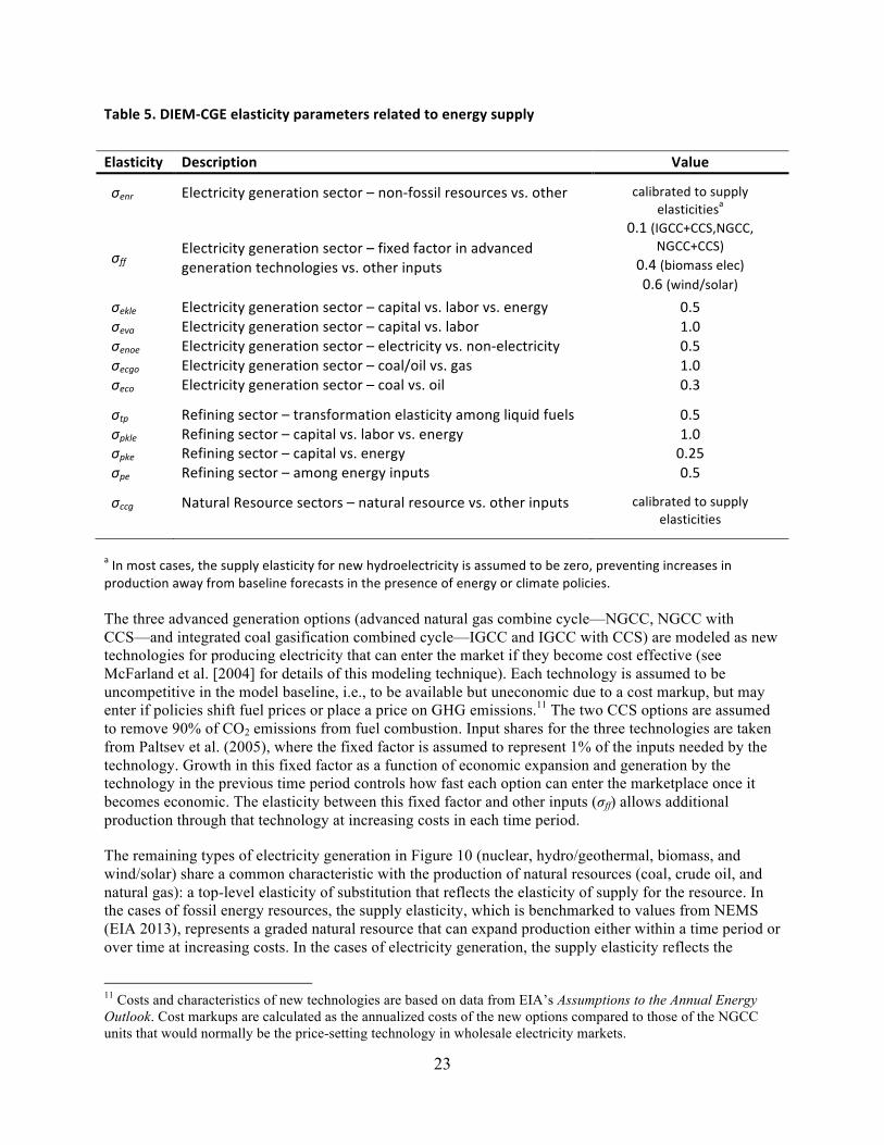
Table 5. DIEM-‐CGE elasticity parameters related to energy supply
Elasticity Description Value σenr Electricity generation sector – non-‐fossil resources vs. other calibrated to supply
elasticitiesa
σff Electricity generation sector – fixed factor in advanced generation technologies vs. other inputs
0.1 (IGCC+CCS,NGCC, NGCC+CCS)
0.4 (biomass elec) 0.6 (wind/solar)
σekle Electricity generation sector – capital vs. labor vs. energy 0.5 σeva Electricity generation sector – capital vs. labor 1.0 σenoe Electricity generation sector – electricity vs. non-‐electricity 0.5 σecgo Electricity generation sector – coal/oil vs. gas 1.0 σeco Electricity generation sector – coal vs. oil 0.3 σtp Refining sector – transformation elasticity among liquid fuels 0.5 σpkle Refining sector – capital vs. labor vs. energy 1.0 σpke Refining sector – capital vs. energy 0.25 σpe Refining sector – among energy inputs 0.5 σccg Natural Resource sectors – natural resource vs. other inputs calibrated to supply
elasticities a In most cases, the supply elasticity for new hydroelectricity is assumed to be zero, preventing increases in production away from baseline forecasts in the presence of energy or climate policies.
The three advanced generation options (advanced natural gas combine cycle—NGCC, NGCC with CCS—and integrated coal gasification combined cycle—IGCC and IGCC with CCS) are modeled as new technologies for producing electricity that can enter the market if they become cost effective (see McFarland et al. [2004] for details of this modeling technique). Each technology is assumed to be uncompetitive in the model baseline, i.e., to be available but uneconomic due to a cost markup, but may enter if policies shift fuel prices or place a price on GHG emissions.11 The two CCS options are assumed to remove 90% of CO2 emissions from fuel combustion. Input shares for the three technologies are taken from Paltsev et al. (2005), where the fixed factor is assumed to represent 1% of the inputs needed by the technology. Growth in this fixed factor as a function of economic expansion and generation by the technology in the previous time period controls how fast each option can enter the marketplace once it becomes economic. The elasticity between this fixed factor and other inputs (σff) allows additional production through that technology at increasing costs in each time period.
The remaining types of electricity generation in Figure 10 (nuclear, hydro/geothermal, biomass, and wind/solar) share a common characteristic with the production of natural resources (coal, crude oil, and natural gas): a top-level elasticity of substitution that reflects the elasticity of supply for the resource. In the cases of fossil energy resources, the supply elasticity, which is benchmarked to values from NEMS (EIA 2013), represents a graded natural resource that can expand production either within a time period or over time at increasing costs. In the cases of electricity generation, the supply elasticity reflects the
11 Costs and characteristics of new technologies are based on data from EIA’s Assumptions to the Annual Energy Outlook. Cost markups are calculated as the annualized costs of the new options compared to those of the NGCC units that would normally be the price-setting technology in wholesale electricity markets.

24
model’s capacity to increase electricity output away from the baseline values in the model at increasing costs in response to policies that incentivize non-fossil generation.
Figure 10. Electricity generation options
Formally, if the production function for fossil energy from Equation 17 in the previous section has the following form (where Yccg is output, Rccg is the resource, Xccg,n are intermediate inputs 1 to n, VAccg is value added, αccg is the share coefficient in the CES equations, and σccg = (1/(1-ρccg)) is the elasticity of substitution):
𝑌!!" = 𝛼!!"𝑅!!"!!!" + 1 − 𝛼!!" 𝑚𝑖𝑛 𝑋!!",!,… ,𝑋!!",!,𝑉𝐴!!"!!!"
! !!!" (21)
then the elasticity of substitution (σccg) at the reference point in the top level sets the price elasticity of supply (ϛccg) according to:
Electricity
Gas
Coal
Capital
σeco
Capital -‐ Labor
Oil
Capital -‐ Labor -‐ Energy
σenoe
σekle
COMg
Electricity
INDg TRNg
Energy
Nuclear -‐ Hydro Biomass -‐ Wind
Capital Labor
Materials
σenr
Resource
σ = ∞
Advanced Technologies
Capital Labor
Materials
σff
Fixed Factor
Conventional Fossil
Labor Non-‐Electricity
Coal-‐Oil
σeva
σecgo

25
𝜍!!" = 𝜎!!"!!!!!"!!!"
(22)
In the baseline setting process discussed in the next section, the wholesale price path for resources is established, and this approach is used to set the supply elasticity around that baseline production forecast.
Petroleum refining is modeled through a special CES function, even though it is not a natural resource sector. It does, however, rely critically on inputs of the homogeneous crude oil commodity. The production structure in Figure 12 allows some limited substitution and energy efficiency improvements, but it uses crude oil in fixed proportions to prevent the model from attempting to turn other types of inputs into refined oil.
Figure 11. Coal, crude oil, and natural gas production: CCG
Figure 12. Refining of petroleum and other liquid fuels: RFP
σccg
Labor
Natural Resource Goods (CCG)
Energy Capital COMg INDg TRNg Natural Resource
σpke
Labor
Liquid Fuels
Capital-‐Labor-‐Energy
Capital-‐Energy
COMg INDg TRNg Crude Oil
σpkle
σtp
Capital Energy
Electricity Gas Oil Coal
σpe

26
DATA AND BASELINE FORECASTS IN DIEM-‐CGE
The model uses a wide range of data sources to characterize the global and U.S. regional economies in the initial model year of 2010. Comprehensive “social accounting matrices” (SAM) of world national and U.S. states (GTAP and IMPLAN, respectively) provide consistent representations of production technologies and outputs, consumption patterns, investments, and trade flows for the relevant regions. The Global Trade Analysis Project also provides some information on international energy consumption and prices, although these data have been updated in DIEM-CGE to the model start year of 2010 using additional data from the International Energy Agency (IEA). Within the United States, similar economic data come from the Minnesota IMPLAN Group, which provides state-level data on economic activity and household income/spending patterns by income group. The household data is augmented with additional information regarding state sales and gasoline taxes and with marginal income tax rates by income source from the NBER TAXSIM model (Feenberg and Coutts 1993). The energy data for U.S. states are replaced with data from EIA (State Energy Data System and Annual Energy Outlook) to better characterize energy markets and provide forecasts for energy consumption and prices. Table 6 summarizes these and other relevant data sources.
Because the DIEM-CGE model is a dynamic model, looking at policy impacts over time, it requires the specification of several types of growth forecasts that extend the initial economic/energy data from the base year of 2010 into the future. These forecasts are provided by a combination of population projections (U.N. 2011; U.S. Census Bureau 2013) and economic/energy forecasts from the World Energy Outlook, (IEA 2012c) and the U.S. Annual Energy Outlook (EIA 2013a). Like other CGE models, DIEM-CGE uses labor growth to drive many of the trends in the model. Growth in the labor force is a combination of changes in the size of the labor force and improvements in labor productivity. Throughout the WEO and AEO forecast periods, the provided GDP growth estimates drive labor growth. After these forecasts end (in 2035 and 2040, respectively), population growth combined with improvements in labor productivity from the ends of the forecast periods are used to extend economic forecasts through 2100.
Incorporation of baseline forecasts for energy consumption by region and economic sector is achieved through the specification of autonomous energy efficiency improvement parameters that adjust energy use per unit of output (see Paltsev et al. 2005). These AEEI parameters represent non-price induced changes in technological progress expected in the model’s baseline. Any price-induced changes in energy consumption due to new policies in the model, however, are estimated endogenously and are controlled by the CES equations detailed in the previous section. Baseline growth in fossil fuels production is imposed on the model as exogenously driven increases in the supplies of natural resources, based on the initial forecasts from AEO and WEO. From this starting path, the model imposes resource supply elasticities that then control any price-induced movements away from this baseline forecast, as discussed previously. Wholesale energy prices are targeted through changes in energy production costs, whereas retail energy prices are targeted through a combination of changes in wholesale prices plus the changes in energy margins (transport and distribution costs) shown in the AEO.

27
Table 6. DIEM-‐CGE data sources Region Type Source Version Data
Internationa
l
Economy Global Trade Analysis Project, Purdue University
Version 8 (year 2007) Narayanan et al. (2012)
Social accounting matrices for 129 regions and 57 commodities; bilateral trade flows, production technologies, household preferences, taxes, etc.
Energy International Energy
Agency Year 2010 (IEA 2012a,b)
Energy consumption by sector/type for year 2010, energy prices (for OECD)
Population United Nations Medium Variant,
2010 (U.N. 2011) International population forecasts through 2100
Forecasts International Energy Agency
World Energy Outlook 2012 (IEA 2012c)
Country/region forecasts of GDP growth, energy use by sector/type, and some energy prices
Non-‐CO2 GHG
U.S. Environmental Protection Agency
Global GHG Emissions (EPA 2012)
Emissions and forecasts of five non-‐CO2 GHG by country and source
United States
Economy Minnesota IMPLAN Group
Year 2010 (IMPLAN 2012)
State-‐level social accounting matrices for 500 commodities in 2010; production technologies, household consumption by income class, some taxes, etc.
Energy U.S Energy Information
Administration State Energy Data System (EIA 2012)
State-‐level data on energy production, consumption and retail prices for 2010
Population U.S. Census Bureau Projections for 2012 (U.S. Census Bureau 2013)
U.S. population projections
Forecasts U.S Energy Information Administration
Annual Energy Outlook 2013 (EIA 2013a)
Regional/national energy production, consumption, and prices; GDP and consumption growth, emissions
Assumptions to Annual Energy Outlook 2013 (EIA 2013b)
Costs and characteristics of new electricity generation options
Households U.S. Bureau of Labor Statistics
Consumer Expenditure Survey, 2011 (BLS 2012)
Annual spending by household income class and type
Taxes
National Bureau of Economic Research
TAXSIM model data for 2010 (Feenberg and Coutts 1993)
State and federal marginal income tax rates by type
Tax Foundation Tax rates for 2010 (Tax Foundation 2013)
State taxes for consumption and gasoline
Non-‐CO2 GHG U.S. Environmental Protection Agency
U.S. GHG Emissions Inventory for 2010 (EPA 2013)
Historical GHG emissions by source

28
GHG EMISSIONS AND ABATEMENT COSTS IN DIEM-‐CGE
In addition to greenhouse gases from burning of fossil fuels, the DIEM-CGE model considers emissions and abatement costs for a variety of non-energy sources. Based on EPA (2012)—global emissions—and EPA (2013)—U.S. emissions, apportioned to states—the model includes initial quantities and forecasts for six greenhouse gases: CO2 from non-energy sources, methane (CH4), nitrous oxide (N2O), hydrofluorocarbons (HFCs), perfluorocarbons (PFCs), and sulfur hexafluoride (SF6). Table 7 shows how gases and emissions sources are assigned to particular sectors in DIEM-CGE.
Non-CO2 emissions are expected to provide a cost-effective means of reducing GHG emissions, especially in the short term. Thus, additional steps are taken to incorporate their abatement options in the model in an endogenous fashion (see Hyman et al. [2003] for an investigation of the implications of these steps). Following Hyman (2001) and Paltsev et al. (2005), emissions in the production structure of the sector responsible them are included at a nominal initial price. The elasticities shown in Table 7 (Paltsev et al. 2005), which are calibrated to abatement costs for each gas in a sector, are then applied in a new top-level CES nest in the sector’s production function to allow firms and households to choose endogenous reductions in emissions by substituting other factors of production. Additional code in the model then allows these emissions sources to be traded off against CO2 emissions from fossil fuels to equilibrate prices across GHG sources (if appropriate for a particular policy). The default metric is the 100-year global warming potential of the gases when trading against each other.

29
Table 7. DIEM-‐CGE data and elasticities for non-‐energy GHG emissions GHG Sources DIEM-‐CGE Sector Elasticity
CO2 (non-‐energy)
Iron & steel, ferroalloy production Iron & steel (I_S, part of EIM) 0 Aluminum, lead, zinc production Non-‐ferrous metals (NFM, part of EIM) 0 Natural gas systems Natural gas production (GAS) 0 Cement, lime, limestone, ammonia production/use Non-‐metallic minerals (NMM, part of EIM) 0 Petrochemical, phosphoric acid, urea, soda ash Chemicals (CHM, part of EIM) 0 Petroleum systems Petroleum refining (OIL) 0 Silicon carbide production/use Electronic equipment (EEQ, part of MAN) 0 Deforestation and biomass burning Crops (CRP, part of AGR) 0 Incineration of waste Residential households (RES) 0
CH4
Natural gas systems Natural gas production (GAS) 0.15 Enteric fermentation and manure Livestock (LIV, part of AGR) 0.05 Landfills, wastewater, composting, waste burning Residential households (RES) 0.11 Coal mining Coal production (COL) 0.30 Petroleum systems Petroleum refining (OIL) 0.15 Rice cultivation, field & biomass burning Crops (CRP, part of AGR) 0.05 Stationary & mobile combustion Fuel use (proportional) 0 Petrochemical production Chemicals (CHM, part of EIM) 0.11 Iron & steel, coke, ferroalloy production Iron & steel (I_S, part of EIM) 0.11 Silicon carbide production Electronic equipment (EEQ, part of MAN) 0.11
N2O
Agricultural soil management & field burning Crops (CRP, part of AGR) 0.03 Stationary & mobile combustion Fuel use (proportional) 0 Manure management Livestock (LIV, part of AGR) 0.03 Nitric & adipic acid, N2O from products Chemicals (CHM, part of EIM) 1.00 Wastewater, composting, waste burning Residential households (RES) 0
HFCs Substitution of ozone-‐depleting substances Industrial machinery (OME, part of MAN) 0.15 HCFC-‐22 production Chemicals (CHM, part of EIM) 0.15 Semiconductor manufacture Electronic equipment (EEQ, part of MAN) 0.15
PFCs
Aluminum production Non-‐Ferrous metals (NFM, part of EIM) 0.30 Semiconductor manufacture Electronic equipment (EEQ, part of MAN) 0.30
SF6 Electrical transmission & distribution Electricity (ELE) 0.30 Semiconductor manufacture Electronic equipment (EEQ, part of MAN) 0.30 Magnesium production & processing Non-‐ferrous metals (NFM, part of EIM) 0.30

30
LINKAGE BETWEEN DIEM-‐CGE AND DIEM-‐ELECTRICITY
It is possible to include a “bottom-up” representation directly within a CGE model solving as a MCP (Bohringer and Rutherford 2008) by representing its Kuhn-Tucker equilibrium conditions, but this approach can quickly become intractable because of dimensionality and the need to include income effects associated upper/lower bounds in the “bottom-up” model. Thus, DIEM uses the block decomposition algorithm proposed in Bohringer and Rutherford (2009) to iterate between the DIEM-CGE and DIEM-Electricity models until a consistent general equilibrium response is achieved in both models.
A critical insight for this approach is that a Marshallian demand approximation for electricity is a good local representation of general equilibrium demands; thus, a rapid convergence between the CGE and electricity models is seen as long as electricity is a small part of the overall economy. This process is illustrated in Figure 13 where P0 and Q0 are an initial guesses of the price and quantity of electricity, P1 and Q1 are the second guess in the iterative algorithm, and P* and Q* are the final converged solutions. To achieve convergence, the objective function in the electricity model must be modified from a cost-minimization approach to include an estimate of the non-linear demand function in the CGE model (points a and b in Figure 13). This task is accomplished by adjusting the objective function in the electricity model to maximize the sum of producer and consumer surplus (area CDE in the figure).
Figure 13. Iterative adjustments in general equilibrium setting
In general terms, the iterative link between the two models involves DIEM-CGE determining for the economy as whole, including the electricity sector, electricity demands (Dele); fuel prices (pf) for coal,
P
P0 P1 P*
Q Q0 Q1 Q*
a b
C
D
E
F DIEM0
DIEM1 ≈ DIEM*

31
natural gas, and petroleum; factor prices for labor (pl) and capital (rk); and any economy-wide CO2 allowance prices (pcarb). The DIEM-Electricity model incorporates these findings as givens and uses them to estimate electricity generation (GEN); fuel demands in electricity (edf), and CO2 emissions from electricity (CO2
ele). A consistent solution between the two models has to agree on all of the results from one iteration to the next. A consistent solution also has to include all producer surplus in electricity generation (area CDF in Figure 13) from submarginal generators in the income of agents in the CGE model. At a unit level, these profits are calculated as the difference between the market price of wholesale electricity (P*), which is set by the marginal cost producer, and the production costs of generators lower than the market price. These producer surpluses arise because of the various capacity, resource, and transmission constraints considered by the electricity model.10
A more formal exposition of the equilibrium conditions in DIEM-Electricity and adjustments to DIEM-CGE follows (see Lanz and Rausch 2011). Electricity generation from each model plant (genp,l) in each block of the load curve (l)11 exhibits complementary slackness with the plant’s zero-profit condition, ignoring regional and time period subscripts:
−𝜋!,! ≥ 0 ⊥ 𝑔𝑒𝑛!,! ≥ 0 (23)
where the unit profit function (ignoring capital investments and carbon costs) is a function of the wholesale electricity price in demand block l (pl
whl), fixed O&M costs (fom), a price index on the fixed costs from the CGE model—assuming for simplicity that all fixed costs are goods (pi), variable O&M costs (vom), a price index on the variable costs from the CGE model—assuming all variable costs are labor (pl), fuel use as a function of unit heat rate—btu per kWh (heatratep), the price of fuel (pf), and scarcity rents for submarginal generators (µp):
𝜋!,! = 𝑝!!!! − 𝑓𝑜𝑚!×𝑝! − 𝑣𝑜𝑚!×𝑝𝑙 − 𝑔𝑒𝑛!,!×ℎ𝑒𝑎𝑡𝑟𝑎𝑡𝑒!×𝑝! − 𝜇!,! (24)
The wholesale electricity price in each demand block (dele) is the complementary variable to the demand constraint:
𝑔𝑒𝑛!,! = 𝑑!!"! ⊥ 𝑝!!!!! (25)
Unit scarcity rents are the complementary variable to the capacity (capp) constraint per load block:
𝑔𝑒𝑛!,! ≤ 𝑐𝑎𝑝!×𝑃𝑙𝑎𝑛𝑡 𝐴𝑣𝑎𝑖𝑙𝑎𝑏𝑖𝑙𝑖𝑡𝑦! ⊥ 𝜇!.! (26)
In DIEM-CGE, a weighted average wholesale electricity price across load blocks is used:
𝑃!"! = !!"#!,!!,!
× 𝑝!!!!×𝑔𝑒𝑛!,!!,! (27)
Within DIEM-Electricity, the objective function includes a demand equation calibrated to annual demands (Dele) and wholesale prices (indicated by bars) as well as an elasticity of demand from DIEM-CGE (ε):
𝐷!"! = 𝐷!"! !!"!
!!"!
! (28)
10 Similar to other capital earnings in DIEM-CGE, in the absence of data on the location of capital ownership, these profits are distributed proportional to other capital income. 11 A benefit of DIEM-Electricity is its capacity to represent multiple demand periods, or blocks, for electricity by season and time of day to better characterize electricity markets and the (generally) non-storable nature of electricity.

32
On the basis of these equations, it is possible to reformulate the market clearance conditions in DIEM-CGE to handle the iterative linkage to DIEM-Electricity, where particular iterations are noted by the index n=1,...,N. In this approach, the CGE model takes electricity supplies as exogenously determined in the electricity model (thus dropping the zero-profit conditions in the CGE model for generation) and includes the estimated factor use by generators in the CGE model’s factor markets:12
𝑔𝑒𝑛!,!(!!!)!,! = 𝐷!"!! ⊥ 𝑃!"!(!) (29)
𝑌!(!) = 𝑦!!!!!!!
+ ! 𝑚!!!"!!!!
(!)+ 𝑐𝑎𝑝!×𝑓𝑜𝑚!!
(!!!) ⊥ 𝑝!(!) (14’)
𝐿(!) = 𝑦!!!!!"#
+! 𝑚!!!"!!"#
(!)+ 𝑔𝑒𝑛!,!×𝑣𝑜𝑚!!,!
(!!!) ⊥ 𝑝𝑙(!) (15’)
And, finally, the household income constraint is modified to include capacity rents:
𝑀! = 𝑝𝑙 ∙ 𝐿!(!) + 𝑟𝑘 ∙ 𝐾!(!) + 𝑔𝑒𝑛!,!(!!!)!,! × 𝑃!"!(!)𝑝!!!!(!!!) − 𝑓𝑜𝑚!×𝑝!(!) −
𝑣𝑜𝑚!×𝑝𝑙(!) − 𝑔𝑒𝑛!,!×ℎ𝑒𝑎𝑡𝑟𝑎𝑡𝑒!×𝑝!(!) (10’)
As noted in Lanz and Rausch (2012), in this approach electricity and inputs to generation are valued at market prices, and thus the capacity rents do not need to appear explicitly in the CGE model.
12 Similar equations also cover fuel markets at price pf and carbon markets at price pcarb.

33
REFERENCES
Armington, P.S. 1969. “A Theory of Demand for Products Distinguished by Place of Production.” IMF Staff Papers 16:159-178.
Arrow, K.J., and G. Debreu. 1954. “Existence of an Equilibrium for a Competitive Economy.” Econometrica 22:265–290.
Arrow, K.J., and F.H. Hahn. 1971. General Competitive Analysis. San Francisco: Holden-Day.
Babiker, M.H., J.M. Reilly, M. Mayer, R.S. Eckaus, I.S. Wing, and R.C. Hyman. 2001. “The MIT Emissions Prediction and Policy Analysis (EPPA) Model: Revisions, Sensitivities, and Comparisons of Results.” MIT Joint Program on the Science and Policy of Global Change, Report No. 71. Cambridge, MA. http://web.mit.edu/globalchange/www/MITJPSPGC_Rpt71.pdf.
Balistreri, E.J., and T.F. Rutherford. 2004. “Assessing the State-level Burden of Carbon Emissions Abatement.” Colorado School of Mines, Golden, CO. http://www.mines.edu/~ebalistr/Papers/CO2004.pdf.
Ballard, C., 2000. How Many Hours Are in a Simulated Day? The Effect of Time Endowment on the Results of Tax-policy Simulation Models. Michigan State University, E. Lansing, MI.
Böhringer, C. 1998. “The Synthesis of Bottom-Up and Top-Down in Energy Policy Modeling.” Energy Economics 20: 233–248.
Böhringer, C., and T.F. Rutherford. 2008. “Combining Bottom-Up and Top-Down.” Energy Economics 30: 574–596.
Böhringer, C., and T.F. Rutherford. 2009. “Integrated Assessment of Energy Policies: Decomposing Top-Down and Bottom-Up.” Journal of Economic Dynamics and Control 33: 1648–1661.
Bovenberg, L.A., and L.H. Goulder. 1996. “Optimal Environmental Taxation in the Presence of Other Taxes: General-Equilibrium Analysis.” American Economic Review 86(4):985–1000.
Bovenberg, A., L. Goulder, and J. Gurney. 2005. “Efficiency Costs of Meeting Industry-Distributional Constraints under Environmental Permits and Taxes.” RAND Journal of Economics 36(4): 951–71.
Feenberg, D., and E. Coutts. 1993. “An Introduction to the TAXSIM Model.” Journal of Policy Analysis and Management 12(1):189–194. http://www.nber.org/~taxsim/.
Fuchs, V.R., A.B. Krueger, and J.M. Poterba. 1998. “Economists’ Views about Parameters, Values, and Policies: Survey Results in Labor and Public Economics.” Journal of Economic Literature 36:1387–1425.
GAMS Development Corporation. 2012. “GAMS: A User’s Guide.” http://www.gams.com/.
Goulder, L.H., Ian W.H. Parry, and D. Burtraw. 1997. “Revenue-Raising Versus Other Approaches to Environmental Protection: The Critical Significance of Preexisting Tax Distortions.” RAND Journal of Economics 28:708–731.
Hyman, R. 2001. “A More Cost-Effective Strategy for Reducing Greenhouse Gas Emissions: Modeling the Impact of Methane Abatement Opportunities.” Master of Science thesis, Technology and Policy Program, MIT, Cambridge, Massachusetts.

34
Hyman, R.C., J.M. Reilly, M.H. Babiker, A. De Masin, and H.D. Jacoby. 2003. “Modeling Non-CO2 Greenhouse Gas Abatement.” Environmental Modeling and Assessment 8: 175–186.
IEA (International Energy Agency). 2012a. “Energy Balances of OECD Countries: 2012.” http://www.iea.org/w/bookshop/add.aspx?id=610.
———. 2012b. “Energy Balances of Non-OECD Countries – 2012.” http://www.iea.org/w/bookshop/add.aspx?id=612.
———. 2012c. “World Energy Outlook – 2012.” http://www.worldenergyoutlook.org/.
Lanz, B., and S. Rausch. 2011. “General Equilibrium, Electricity Generation Technologies and the Cost of Carbon Abatement: A Structural Sensitivity Analysis.” Energy Economics 33: 1035–1047.
Lau, M., A. Pahlke, and T. Rutherford. 2002. “Approximating Infinite-Horizon Models in a Complementarity Format: A Primer in Dynamic General Equilibrium Analysis.” Journal of Economic Dynamics and Control 26(4):577–609.
Mathiesen, L. 1985. “Computation of Economic Equilibrium by a Sequence of Linear Complementarity Problems.” Mathematical Programming Study 23: 144–162.
McFarland, J., J. Reilly, and H.J. Herzog. 2004. “Representing Energy Technologies in Top-Down Economic Models Using Bottom-Up Information.” Energy Economics 26: 685–707.
Minnesota IMPLAN Group. 2012. “State-Level U.S. Data for 2010.” Stillwater, Minnesota: Minnesota IMPLAN Group.
Narayanan, G., A. Aguiar Badri, and R. McDougall, eds. 2012. Global Trade, Assistance, and Production: The GTAP 8 Data Base. Center for Global Trade Analysis, Purdue University.
Paltsev, S., J.M Reilly, H.D. Jacoby, R.S. Eckaus, J. McFarland, M. Sarofim, M. Asadoorian, and M. Babiker. 2005. “The MIT Emissions Prediction and Policy Analysis (EPPA) Model: Version 4.” MIT Joint Program on the Science and Policy of Climate Change, Report 125.
Parry, Ian W.H., and A.M. Bento. 2000. “Tax Deductions, Environmental Policy, and the ‘Double Dividend’ Hypothesis.” Journal of Environmental Economics and Management 39:67–96.
Phelps, E.S. 1963. “Substitution, Fixed Proportions, Growth and Distribution.” International Economic Review 4:265–288.
Rausch, S., G.E. Metcalf, J.M. Reilly, and S. Paltsev. 2009. “Distributional Impacts of a U.S. Greenhouse Gas Policy: A General Equilibrium Analysis of Carbon Pricing.” MIT Joint Program on the Science and Policy of Climate Change, Report 182.
Rausch, S., and M. Mowers. 2012. “Distributional and Efficiency Impacts of Clean and Renewable Energy Standards for Electricity.” MIT Joint Program on the Science and Policy of Climate Change, Report 225.
Ross, M.T. 2014. “Structure of the Dynamic Integrated Economy/Energy/Emissions Model: Electricity Component, DIEM-Electricity.” NI WP 14-11. Durham, NC: Duke University.
35
Russek, F.S. 1996. “Labor Supply and Taxes.” Congressional Budget Office, Washington D.C. ftp://ftp.cbo.gov/33xx/doc3372/labormkts.pdf.
Rutherford, T.F. 1995. “Extension of GAMS for Complementarity Problems Arising in Applied Economic Analysis.” Journal of Economic Dynamics and Control 19(8): 1299–1324.
Rutherford, T.F. 1999. “Applied General Equilibrium Modeling with MPSGE as a GAMS Subsystem: An Overview of the Modeling Framework and Syntax.” Computational Economics 14(1):1–46.
Rutherford, T.F. 2004. “Tools for Building National Economic Models Using State-Level IMPLAN Social Accounts.” University of Colorado, Boulder, Colorado. http://debreu.colorado.edu/implan98.htm.
Stavins, R.N. 2008. “A Meaningful U.S. Cap-and-Trade System to Address Climate Change.” Harvard Environmental Law Review 32: 293–371.
The Tax Foundation. 2013a. “State General Sales and Use Tax Rates.” Accessed May 15, 2013. http://www.taxfoundation.org/.
———. 2013b. “State Corporate Income Tax Rates.” Accessed May 15, 2013. http://www.taxfoundation.org/.
———. 2013c. “State Gasoline Tax Rates.” Accessed May 15, 2013. http://www.taxfoundation.org.
United Nations. 2011. “World Population Prospects: The 2010 Revision.” United Nations, New York, NY. Accessed May 15, 2013. http://esa.un.org/wpp/Documentation/publications.htm.
BLS (U.S. Bureau of Labor Statistics). 2012. Consumer Expenditure Survey. Accessed May 15, 2013. http://www.bls.gov/cex/.
U.S. Census Bureau. 2013. “Population Projections.” Accessed May 15, 2013. http://www.census.gov/population/projections/.
EIA (U.S. Energy Information Administration). 2009. “The National Energy Modeling System: An Overview 2009.” DOE/EIA-0581(2009).
———. 2012. “State Energy Data System.” Accessed May 15, 2013. http://www.eia.gov/state/seds/.
———. 2013a. “Annual Energy Outlook 2013.” Accessed May 15, 2013. http://www.eia.gov/forecasts/aeo/.
———. 2013b. “Assumptions to the Annual Energy Outlook.” Accessed May 15, 2013. http://www.eia.gov/forecasts/aeo/assumptions/index.cfm.
EPA (U.S Environmental Protection Agency). 2012. “Global Anthropogenic Non-CO2 Greenhouse Gas Emissions: 1990–2030.” EPA #430-R-12-006. Accessed May 15, 2013. http://www.epa.gov/climatechange/EPAactivities/economics/nonco2projections.html.
———. 2013. “Inventory of U.S. Greenhouse Gas Emissions and Sinks: 1990–2011 (April 2013).” EPA #430-R-13-001. Accessed May 15, 2013. http://www.epa.gov/climatechange/ghgemissions/usinventoryreport.html.

36
Williams, Roberton C., III. 1999. “Revisiting the Cost of Protectionism: The Role of Tax Distortions in the Labor Market.” Journal of International Economics 47:429–447.