Embed Size (px)
Citation preview
!!!
!!!
!!!
!!!
!!!
!!!
!!!
!!!
!!!
!!!
!!!
!!!
!!!
!!!
!!!
!!!
!!!
!!!
!!!
!!!
!!!
!!!
!!!
!!!
!!!
!!!
!!!
!!!
!!!
!!!
!!!
!!!
!!!
!!!
!!!
!!!
!!!
!!!
!!!
!!!
!!!
!!!
!!!
!!!
!!!
!!!
!!!
!!!
!!!
!!!
!!!
!!!
!!!
!!!
!!!
!!!
!!!
!!!
!!!
!!!
!!!
!!!
!!!
!!!
!!!
!!!
!!!
!!!
!!!
!!!
!!!
!!!
!!!
!!!
!!!
!!!
!!!
!!!
!!!
!!!
!!!
!!!
!!!
!!!
!!!
!!!
!!!
!!! EidgenossischeTechnische Hochschule
Zurich
Ecole polytechnique federale de ZurichPolitecnico federale di Zurigo
Swiss Federal Institute of Technology Zurich
Structured eigenvalue condition numbers andlinearizations for matrix polynomials
B. Adhikari!, R. Alam† and D. Kressner
Research Report No. 2009-01January 2009
Seminar fur Angewandte MathematikEidgenossische Technische Hochschule
CH-8092 ZurichSwitzerland
!Department of Mathematics, Indian Institute of Technology Guwahati, India, E-mail:[email protected]
†Department of Mathematics, Indian Institute of Technology Guwahati, India, E-mail:[email protected], [email protected], Fax: +91-361-2690762/2582649.
Structured eigenvalue condition numbers andlinearizations for matrix polynomials
Bibhas Adhikari! Rafikul Alam† Daniel Kressner‡.
Abstract. This work is concerned with eigenvalue problems for structured matrix polynomials,
including complex symmetric, Hermitian, even, odd, palindromic, and anti-palindromic matrix poly-
nomials. Most numerical approaches to solving such eigenvalue problems proceed by linearizing the
matrix polynomial into a matrix pencil of larger size. Recently, linearizations have been classified
for which the pencil reflects the structure of the original polynomial. A question of practical impor-
tance is whether this process of linearization increases the sensitivity of the eigenvalue with respect
to structured perturbations. For all structures under consideration, we show that this is not the
case: there is always a linearization for which the structured condition number of an eigenvalue does
not di!er significantly. This implies, for example, that a structure-preserving algorithm applied to
the linearization fully benefits from a potentially low structured eigenvalue condition number of the
original matrix polynomial.
Keywords. Eigenvalue problem, matrix polynomial, linearization, structured condition num-ber.
AMS subject classification(2000): 65F15, 15A57, 15A18, 65F35.
1 Introduction
Consider an n! n matrix polynomial
P(!) = A0 + !A1 + !2A2 + · · · + !mAm, (1)
with A0, . . . , Am " Cn!n. An eigenvalue ! " C of P, defined by the relation det(P(!)) = 0,is called simple if ! is a simple root of the polynomial det(P(!)).
This paper is concerned with the sensitivity of a simple eigenvalue ! under perturbationsof the coe!cients Ai. The condition number of ! is a first-order measure for the worst-casee"ect of perturbations on !. Tisseur [33] has provided an explicit expression for this conditionnumber. Subsequently, this expression was extended to polynomials in homogeneous form byDedieu and Tisseur [9], see also [1, 5, 8], and to semi-simple eigenvalues in [22]. In themore general context of nonlinear eigenvalue problems, the sensitivity of eigenvalues andeigenvectors has been investigated in, e.g., [3, 24, 25, 26].
Loosely speaking, an eigenvalue problem (1) is called structured if there is some distinctivestructure among the coe!cients A0, . . . , Am. For example, much of the recent research onstructured polynomial eigenvalue problems was motivated by the second-order T -palindromiceigenvalue problem [18, 27]
A0 + !A1 + !2AT0 ,
where A1 is complex symmetric: AT1 = A1. In this paper, we consider the structures listed
in Table 1. To illustrate the notation of this table, consider a T -palindromic polynomial!Department of Mathematics, Indian Institute of Technology Guwahati, India, E-mail: [email protected]†Department of Mathematics, Indian Institute of Technology Guwahati, India, E-mail: [email protected],
[email protected], Fax: +91-361-2690762/2582649.‡Seminar for Applied Mathematics, ETH Zurich, Switzerland. E-mail: [email protected]
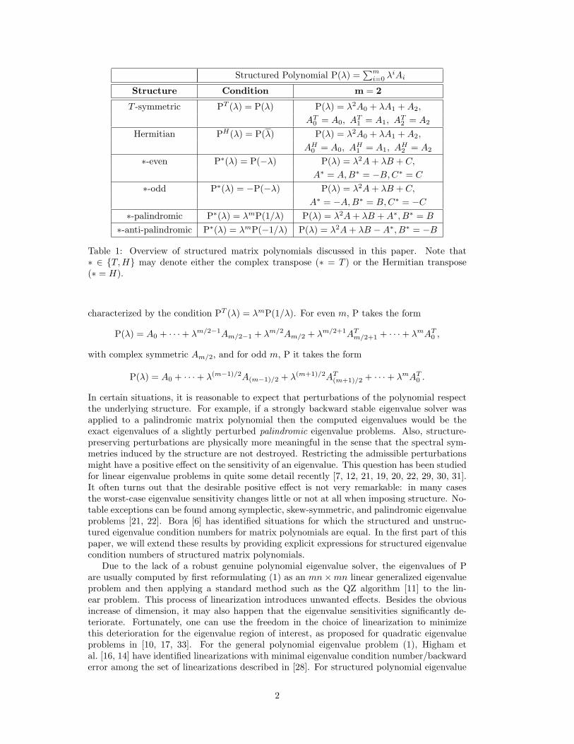
Structured Polynomial P(!) =!m
i=0 !iAi
Structure Condition m = 2
T -symmetric PT (!) = P(!) P(!) = !2A0 + !A1 + A2,
AT0 = A0, AT
1 = A1, AT2 = A2
Hermitian PH(!) = P(!) P(!) = !2A0 + !A1 + A2,
AH0 = A0, AH
1 = A1, AH2 = A2
#-even P"(!) = P($!) P(!) = !2A + !B + C,
A" = A, B" = $B, C" = C
#-odd P"(!) = $P($!) P(!) = !2A + !B + C,
A" = $A, B" = B, C" = $C
#-palindromic P"(!) = !mP(1/!) P(!) = !2A + !B + A", B" = B
#-anti-palindromic P"(!) = !mP($1/!) P(!) = !2A + !B $A", B" = $B
Table 1: Overview of structured matrix polynomials discussed in this paper. Note that# " {T, H} may denote either the complex transpose (# = T ) or the Hermitian transpose(# = H).
characterized by the condition PT (!) = !mP(1/!). For even m, P takes the form
P(!) = A0 + · · · + !m/2#1Am/2#1 + !m/2Am/2 + !m/2+1ATm/2+1 + · · · + !mAT
0 ,
with complex symmetric Am/2, and for odd m, P it takes the form
P(!) = A0 + · · · + !(m#1)/2A(m#1)/2 + !(m+1)/2AT(m+1)/2 + · · · + !mAT
0 .
In certain situations, it is reasonable to expect that perturbations of the polynomial respectthe underlying structure. For example, if a strongly backward stable eigenvalue solver wasapplied to a palindromic matrix polynomial then the computed eigenvalues would be theexact eigenvalues of a slightly perturbed palindromic eigenvalue problems. Also, structure-preserving perturbations are physically more meaningful in the sense that the spectral sym-metries induced by the structure are not destroyed. Restricting the admissible perturbationsmight have a positive e"ect on the sensitivity of an eigenvalue. This question has been studiedfor linear eigenvalue problems in quite some detail recently [7, 12, 21, 19, 20, 22, 29, 30, 31].It often turns out that the desirable positive e"ect is not very remarkable: in many casesthe worst-case eigenvalue sensitivity changes little or not at all when imposing structure. No-table exceptions can be found among symplectic, skew-symmetric, and palindromic eigenvalueproblems [21, 22]. Bora [6] has identified situations for which the structured and unstruc-tured eigenvalue condition numbers for matrix polynomials are equal. In the first part of thispaper, we will extend these results by providing explicit expressions for structured eigenvaluecondition numbers of structured matrix polynomials.
Due to the lack of a robust genuine polynomial eigenvalue solver, the eigenvalues of Pare usually computed by first reformulating (1) as an mn!mn linear generalized eigenvalueproblem and then applying a standard method such as the QZ algorithm [11] to the lin-ear problem. This process of linearization introduces unwanted e"ects. Besides the obviousincrease of dimension, it may also happen that the eigenvalue sensitivities significantly de-teriorate. Fortunately, one can use the freedom in the choice of linearization to minimizethis deterioration for the eigenvalue region of interest, as proposed for quadratic eigenvalueproblems in [10, 17, 33]. For the general polynomial eigenvalue problem (1), Higham etal. [16, 14] have identified linearizations with minimal eigenvalue condition number/backwarderror among the set of linearizations described in [28]. For structured polynomial eigenvalue
2
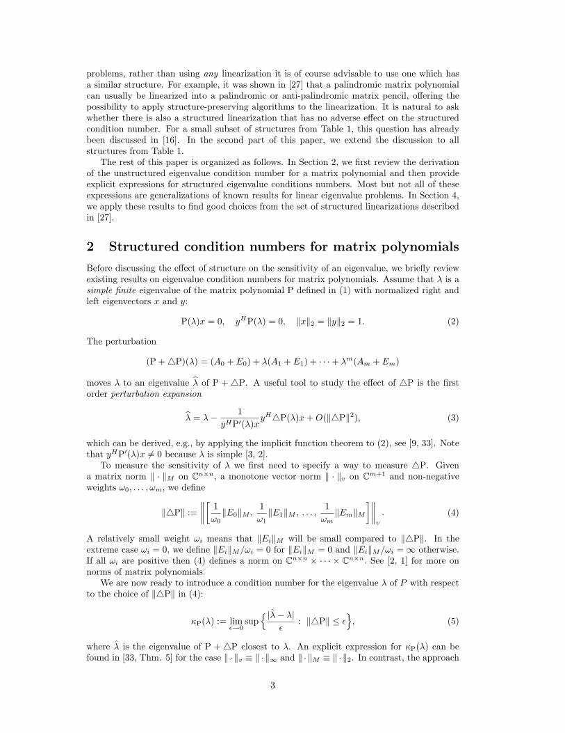
problems, rather than using any linearization it is of course advisable to use one which hasa similar structure. For example, it was shown in [27] that a palindromic matrix polynomialcan usually be linearized into a palindromic or anti-palindromic matrix pencil, o"ering thepossibility to apply structure-preserving algorithms to the linearization. It is natural to askwhether there is also a structured linearization that has no adverse e"ect on the structuredcondition number. For a small subset of structures from Table 1, this question has alreadybeen discussed in [16]. In the second part of this paper, we extend the discussion to allstructures from Table 1.
The rest of this paper is organized as follows. In Section 2, we first review the derivationof the unstructured eigenvalue condition number for a matrix polynomial and then provideexplicit expressions for structured eigenvalue conditions numbers. Most but not all of theseexpressions are generalizations of known results for linear eigenvalue problems. In Section 4,we apply these results to find good choices from the set of structured linearizations describedin [27].
2 Structured condition numbers for matrix polynomials
Before discussing the e"ect of structure on the sensitivity of an eigenvalue, we briefly reviewexisting results on eigenvalue condition numbers for matrix polynomials. Assume that ! is asimple finite eigenvalue of the matrix polynomial P defined in (1) with normalized right andleft eigenvectors x and y:
P(!)x = 0, yHP(!) = 0, %x%2 = %y%2 = 1. (2)
The perturbation
(P +&P)(!) = (A0 + E0) + !(A1 + E1) + · · · + !m(Am + Em)
moves ! to an eigenvalue "! of P +&P. A useful tool to study the e"ect of &P is the firstorder perturbation expansion
"! = !$ 1yHP$(!)x
yH&P(!)x + O(%&P%2), (3)
which can be derived, e.g., by applying the implicit function theorem to (2), see [9, 33]. Notethat yHP$(!)x '= 0 because ! is simple [3, 2].
To measure the sensitivity of ! we first need to specify a way to measure &P. Givena matrix norm % · %M on Cn!n, a monotone vector norm % · %v on Cm+1 and non-negativeweights "0, . . . ,"m, we define
%&P% :=####
$1"0%E0%M ,
1"1%E1%M , . . . ,
1"m
%Em%M
%####v
. (4)
A relatively small weight "i means that %Ei%M will be small compared to %&P%. In theextreme case "i = 0, we define %Ei%M/"i = 0 for %Ei%M = 0 and %Ei%M/"i = ( otherwise.If all "i are positive then (4) defines a norm on Cn!n ! · · · ! Cn!n. See [2, 1] for more onnorms of matrix polynomials.
We are now ready to introduce a condition number for the eigenvalue ! of P with respectto the choice of %&P% in (4):
#P(!) := lim!%0
sup& |!$ !|
$: %&P% ) $
', (5)
where ! is the eigenvalue of P +&P closest to !. An explicit expression for #P(!) can befound in [33, Thm. 5] for the case % ·%v * % · %& and % ·%M * % · %2. In contrast, the approach
3
used in [9] requires an accessible geometry on the perturbation space and thus facilitates thenorms % · %v * % · %2 and % · %M * % · %F . Lemma 2.1 below is more general and includes bothsettings. Note that an alternative approach to the result of Lemma 2.1 is described in [1],admitting any matrix norm % · %M and any (Holder) p-norm % · %V * % · %p. For stating ourresult, we recall that the dual to the vector norm % · %v is defined as
%w%d := sup'z'v(1
|wT z|,
see, e.g., [13].
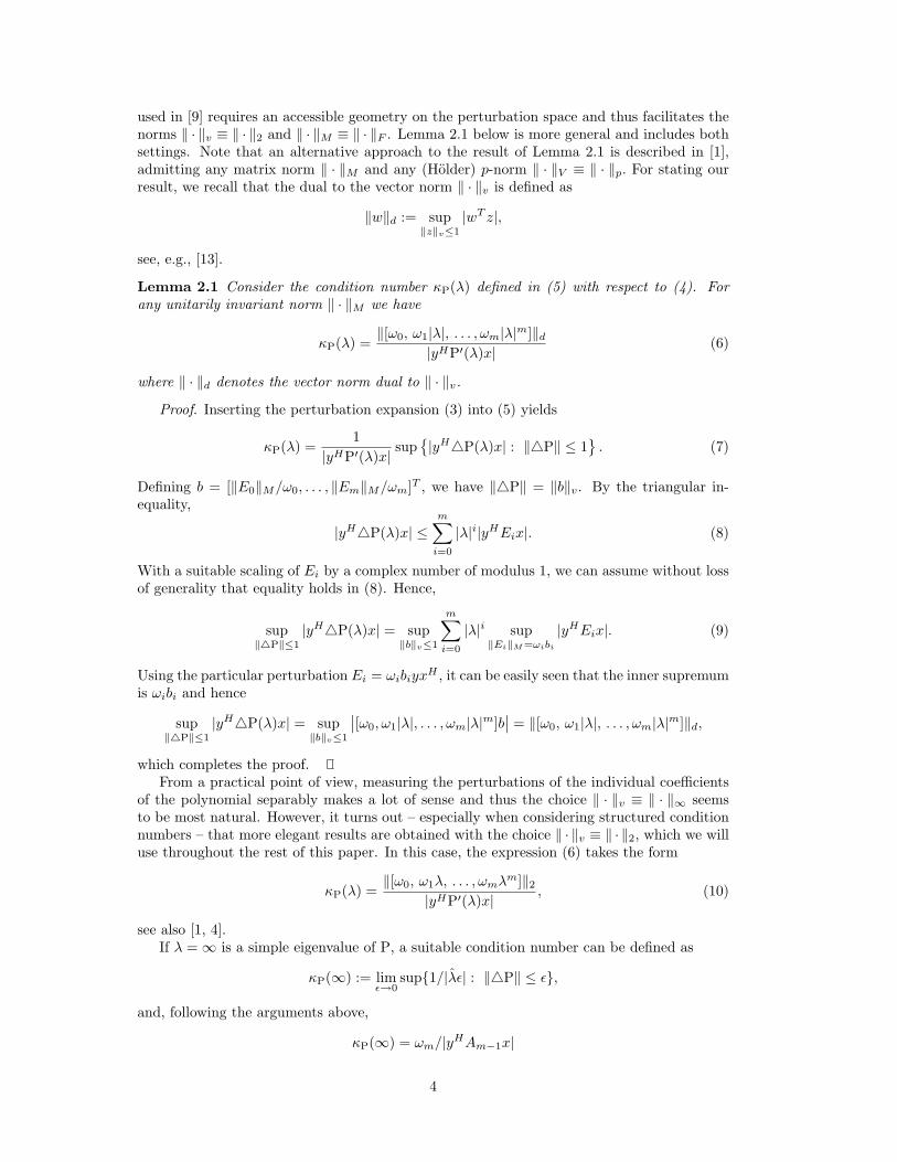
Lemma 2.1 Consider the condition number #P(!) defined in (5) with respect to (4). Forany unitarily invariant norm % · %M we have
#P(!) =%["0, "1|!|, . . . , "m|!|m]%d
|yHP$(!)x| (6)
where % · %d denotes the vector norm dual to % · %v.
Proof. Inserting the perturbation expansion (3) into (5) yields
#P(!) =1
|yHP$(!)x| sup(|yH&P(!)x| : %&P% ) 1
). (7)
Defining b = [%E0%M/"0, . . . , %Em%M/"m]T , we have %&P% = %b%v. By the triangular in-equality,
|yH&P(!)x| )m*
i=0
|!|i|yHEix|. (8)
With a suitable scaling of Ei by a complex number of modulus 1, we can assume without lossof generality that equality holds in (8). Hence,
sup')P'(1
|yH&P(!)x| = sup'b'v(1
m*
i=0
|!|i sup'Ei'M="ibi
|yHEix|. (9)
Using the particular perturbation Ei = "ibiyxH , it can be easily seen that the inner supremumis "ibi and hence
sup')P'(1
|yH&P(!)x| = sup'b'v(1
++["0, "1|!|, . . . ,"m|!|m]b++ = %["0, "1|!|, . . . , "m|!|m]%d,
which completes the proof.From a practical point of view, measuring the perturbations of the individual coe!cients
of the polynomial separably makes a lot of sense and thus the choice % · %v * % · %& seemsto be most natural. However, it turns out – especially when considering structured conditionnumbers – that more elegant results are obtained with the choice % · %v * % · %2, which we willuse throughout the rest of this paper. In this case, the expression (6) takes the form
#P(!) =%["0, "1!, . . . , "m!m]%2
|yHP$(!)x| , (10)
see also [1, 4].If ! = ( is a simple eigenvalue of P, a suitable condition number can be defined as
#P(() := lim!%0
sup{1/|!$| : %&P% ) $},
and, following the arguments above,
#P(() = "m/|yHAm#1x|
4
for any p-norm % · %v. Note that this discrimination between finite and infinite disappearswhen homogenizing P as in [9] or measuring the distance between perturbed eigenvalues withthe chordal metric as in [32]. In order to keep the presentation simple, we have decided notto use these concepts.
The rest of this section is concerned with quantifying the e"ect on the condition numberif we restrict the perturbation &P to a subset S of the space of all n! n matrix polynomialsof degree at most m.
Definition 2.2 Let ! be a simple finite eigenvalue of a matrix polynomial P with normalizedright and left eigenvectors x and y. Then the structured condition number of ! with respectto S is defined as
#SP(!) := lim
!%0sup
,|!$ !|
$: &P " S, %&P% ) $
-(11)
For infinite !, #SP(() := lim
!%0sup{1/|!$| : &P " S, %&P% ) $}.
If S is star-shaped, the expansion (3) can be used to show
#SP(!) =
1|yHP$(!)x| sup
(|yH&P(!)x| : &P " S, %&P% ) 1
)(12)
and#S
P(() =1
|yHAm#1x|sup
(|yHEmx| : &P " S, %Em%M ) "m
). (13)
2.1 Structured first-order perturbation sets
To proceed from (12) we need to find the maximal absolute magnitude of elements from theset (
yH&P(!)x = yHE0x + !yHE1x + · · ·!myHEmx : &P " S, %&P% ) 1)
(14)
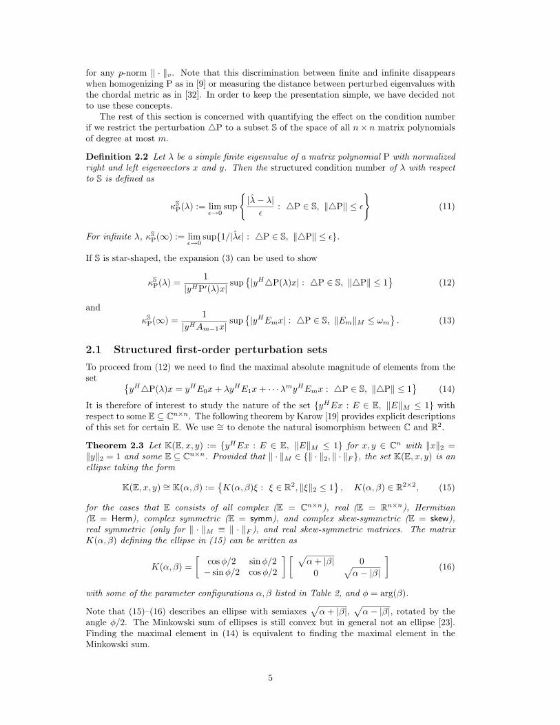
It is therefore of interest to study the nature of the set {yHEx : E " E, %E%M ) 1} withrespect to some E + Cn!n. The following theorem by Karow [19] provides explicit descriptionsof this set for certain E. We use ,= to denote the natural isomorphism between C and R2.
Theorem 2.3 Let K(E, x, y) := {yHEx : E " E, %E%M ) 1} for x, y " Cn with %x%2 =%y%2 = 1 and some E + Cn!n. Provided that % · %M " {% · %2, % · %F }, the set K(E, x, y) is anellipse taking the form
K(E, x, y) ,= K(%,&) :=(K(%,&)' : ' " R2, %'%2 ) 1
), K(%,&) " R2!2, (15)
for the cases that E consists of all complex (E = Cn!n), real (E = Rn!n), Hermitian(E = Herm), complex symmetric (E = symm), and complex skew-symmetric (E = skew),real symmetric (only for % · %M * % · %F ), and real skew-symmetric matrices. The matrixK(%,&) defining the ellipse in (15) can be written as
K(%,&) =$
cos (/2 sin (/2$ sin(/2 cos (/2
% $ .% + |&| 0
0.
%$ |&|
%(16)
with some of the parameter configurations %,& listed in Table 2, and ( = arg(&).
Note that (15)–(16) describes an ellipse with semiaxes.
% + |&|,.
%$ |&|, rotated by theangle (/2. The Minkowski sum of ellipses is still convex but in general not an ellipse [23].Finding the maximal element in (14) is equivalent to finding the maximal element in theMinkowski sum.
5
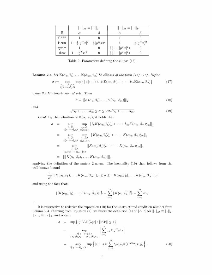
% · %M * % · %2 % · %M * % · %F
E % & % &
Cn!n 1 0 1 0Herm 1$ 1
2 |yHx|2 1
2 (yHx)2 12
12 (yHx)2
symm 1 0 12 (1 + |yT x|2) 0
skew 1$ |yT x|2 0 12 (1$ |yT x|2) 0
Table 2: Parameters defining the ellipse (15).
Lemma 2.4 Let K(%0, &0), . . . , K(%m, &m) be ellipses of the form (15)–(16). Define
) := supb0,...,bm!R
b20+···+b2m"1
sup(%s%2 : s " b0K(%0, &0) + · · · + bmK(%m, &m)
)(17)
using the Minkowski sum of sets. Then
) = %[K(%0, &0), . . . ,K(%m, &m)]%2, (18)
and -%0 + · · · + %m ) ) )
-2-
%0 + · · · + %m. (19)
Proof. By the definition of K(%j , &j), it holds that
) = supbi!R
b20+···+b2m"1
sup!i!R2#!i#2"1
##b0K(%0, &0)'0 + · · · + bmK(%m, &m)'m
##2
= supbi!R
b20+···+b2m"1
sup!i!R2
#!i#2"bi
##K(%0, &0)'0 + · · · + K(%m, &m)'m
##2
= sup!i!R2
#!0#22+···+#!m#22"1
##K(%0, &0)'0 + · · · + K(%m, &m)'m
##2
=##/
K(%0, &0), . . . , K(%m, &m)0##
2,
applying the definition of the matrix 2-norm. The inequality (19) then follows from thewell-known bound
1-2%[K(%0, &0), . . . ,K(%m, &m)]%F ) ) ) %[K(%0, &0), . . . ,K(%m, &m)]%F
and using the fact that:
%[K(%0, &0), . . . ,K(%m, &m)]%2F =m*
i=0
%K(%i, &i)%2F =m*
i=0
2%i.
It is instructive to rederive the expression (10) for the unstructured condition number fromLemma 2.4. Starting from Equation (7), we insert the definition (4) of %&P% for %·%M * %·%2,% · %v * % · %2, and obtain
) = sup(|yH&P(!)x| : %&P% ) 1
)
= supb20+···+b2m"1
#E0#2"b0,...,#Em#2"bm
+++m*
i=0
"i!iyHEix
+++
= supb20+···+b2m(1
sup&|s| : s "
m*
i=0
bi"i!iK(Cn!n, x, y)'
. (20)
6
By Theorem 2.3, K(Cn!n, x, y) ,= K(1, 0) and, since a disk is invariant under rotation,"i!iK(Cn!n, x, y) ,= K("2
i |!|2i, 0). Applying Lemma 2.4 yields
) =##/
K("20 , 0), K("2
1 |!|2, 0), . . . ,K("2m|!|2m, 0)
0##2
=##/
"0, "1!, . . . ,"m!m0##
2,
which together with (7) results in the known expression (10) for #P(!).In the following sections, it will be shown that the expressions for structured condition
numbers follow in a similar way as corollaries from Lemma 2.4. To keep the notation compact,we define
)SP(!) = sup
(|yH&P(!)x| : &P " S, %&P% ) 1
).
for a star-shaped structure S. By (12), #SP(!) = )S
P(!)/|yHP$(!)x|. Let us recall that thevector norm underlying the definition of %&P% in (4), is chosen as % · %v * % · %2 throughoutthe rest of this paper.
2.2 Complex symmetric matrix polynomials
No or only an insignificant decrease of the condition number can be expected when imposingcomplex symmetries on the perturbations of a matrix polynomial.
Corollary 2.5 Let S denote the set of complex symmetric matrix polynomials. Then for afinite or infinite, simple eigenvalue ! of a matrix polynomial P " S,
1. #SP(!) = #P(!) for % · %M * % · %2, and
2. #SP(!) =
-1+|yT x|2*
2#P(!) for % · %M * % · %F .
Proof. Along the line of arguments leading to (20),
)SP(!) = sup
b20+···+b2m(1
&%s%2 : s "
m*
i=0
bi"i!iK(symm, x, y)
'
for finite !. As in the unstructured case, K(symm, x, y) ,= K(1, 0) for % · %M * % · %2 byTheorem 2.3, and thus #P(!) = #S
P(!). For % · %M * % · %F we have
K(symm, x, y) ,= K((1 + |yT x|2)/2, 0) =.
1 + |yT x|2-2
K(1, 0),
showing the second part of the statement. The proof for infinite ! is entirely analogous.
2.3 T -even and T -odd matrix polynomials
To describe the structured condition numbers for T -even and T -odd polynomials in a conve-nient manner, we introduce the vector
#" =/"m!m, "m#1!
m#1, . . . , "1!, "0
0T (21)
along with the even coe!cient projector
$e : #" ./ $e(#") :=
, /"m!m, 0, "m#2!m#2, 0, . . . , "2!2, 0, "0
0T, if m is even,/
0, "m#1!m#1, 0, "m#3!m#3, . . . , 0, "0
0T, if m is odd.
(22)
The odd coe!cient projection is defined analogously and can be written as (1$$e)(#").
Lemma 2.6 Let S denote the set of all T -even matrix polynomials. Then for a finite, simpleeigenvalue ! of a matrix polynomial P " S,
7
1. #SP(!) =
11$ |yT x|2 '(1#!e)("")'22
'""'22#P(!) for % · %M * % · %2, and
2. #SP(!) = 1*
2
11$ |yT x|2 '(1#!e)("")'22#'!e("")'22
'""'22#P(!) for % · %M * % · %F .
For an infinite, simple eigenvalue,
3. #SP(() =
2#P((), if m is even,.
1$ |yT x|2 #P ((), if m is odd,for % · %M * % · %2, and
4. #SP(() =
,1*2
.1 + |yT x|2#P((), if m is even,
1*2
.1$ |yT x|2#P((), if m is odd,
for % · %M * % · %F .
Proof. By definition, the even coe!cients of a T -even polynomial are symmetric while theodd coe!cients are skew-symmetric. Thus, for finite !,
)SP(!) = sup
b20+···+b2m(1sup
&%s%2 : s "
*
i even
bi"i!iK(symm, x, y) +
*
i odd
bi"i!iK(skew, x, y)
'.
Applying Theorem 2.3 and Lemma 2.4 yields for % · %M * % · %2,
)SP(!) =
###3$e(#")T 0K(1, 0), (1$$e)(#")T 0K(1$ |yT x|2, 0)
4###2
=###3$e(#")T ,
11$ |yT x|2(1$$e)(#")T
4###2
=1%#"%22 $ |yT x|2%(1$$e)(#")%22,
once again using the fact that a disk is invariant under rotation. Similarly, it follows for% · %M * % · %F that
)SP(!) =
1-2
###31
1 + |yT x|2$e(#")T ,1
1$ |yT x|2(1$$e)(#")T4###
2
=1-2
1%#"%22 + |yT x|2
5%$e(#")%22 $ %(1$$e)(#")%22
6.
The result for infinite ! follows in an analogous manner.
Remark 2.7 Note that the statement of Lemma 2.6 does not assume that P itself is T -even.If we impose this condition then, for odd m, P has a simple infinite eigenvalue only if alsothe size of P is odd, see, e.g., [22]. In this case, the skew-symmetry of Am forces the infiniteeigenvalue to be preserved under arbitrary structure-preserving perturbations. This is reflectedby #S
P(() = 0.
Lemma 2.6 reveals that the structured condition number can only be significantly lowerthan the unstructured one if |yT x| and the ratio
%(1$$e)(#")%22%#"%22
=
!i odd
"2i |!|2i
!i=0,...,m
"2i |!|2i
= 1$
!i even
"2i |!|2i
!i=0,...,m
"2i |!|2i
are close to one. The most likely situation for the latter ratio to become close to one is whenm is odd, "m does not vanish, and |!| is large.
Example 2.8 ([31]) Let
P(!) = I + !0 + !2I + !3
7
80 1$ ( 0
$1 + ( 0 i0 $i 0
9
:
8
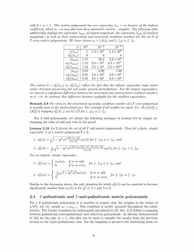
with 0 < ( < 1. This matrix polynomial has one eigenvalue !& = ( because of the highestcoe!cient, which is – as any odd-sized skew-symmetric matrix – singular. The following tableadditionally displays the eigenvalue !max of largest magnitude, the eigenvalue !min of smallestmagnitude, as well as their unstructured and structured condition numbers for the set S ofT -even matrix polynomials. We have chosen "i = %Ai%2 and % · %M * % · %2.
( 100 10#3 10#9
#(!&) 1 1.4! 103 1.4! 109
#SP(!&) 0 0 0|!max| 1.47 22.4 2.2! 104
#P(!max) 1.12 3.5! 105 3.5! 1017
#SP(!max) 1.12 2.5! 104 2.5! 1013
|!min| 0.83 0.99 1.00#P(!min) 0.45 5.0! 102 5.0! 108
#SP(!min) 0.45 3.5! 102 3.5! 108
The entries 0 = #SP(!&) 1 #S
P(!&) reflect the fact that the infinite eigenvalue stays intactunder structure-preserving but not under general perturbations. For the largest eigenvalues,we observe a significant di"erence between the structured and unstructured condition numbersas ( / 0. In contrast, this di"erence becomes negligible for the smallest eigenvalues.
Remark 2.9 For even m, the structured eigenvalue condition number of a T -even polynomialis usually close to the unstructured one. For example if all weights are equal, %(1$$e)(#)%22 )%#%22/2 implying #S
P(!) 2 #P(!)/-
2 for % · %M * % · %2.
For T -odd polynomials, we obtain the following analogue of Lemma 2.6 by simply ex-changing the roles of odd and even in the proof.
Lemma 2.10 Let S denote the set of all T -odd matrix polynomials. Then for a finite, simpleeigenvalue ! of a matrix polynomial P " S,
1. #SP(!) =
11$ |yT x|2 '!e("")'22
'""'22#P(!) for % · %M * % · %2, and
2. #SP(!) = 1*
2
11$ |yT x|2 '!e("")'22#'(1#!e)("")'22
'""'22#P(!) for % · %M * % · %F .
For an infinite, simple eigenvalue,
3. #SP(() =
2#P((), if m is odd,0, if m is even, for % · %M * % · %2, and
4. #SP(() =
,1*2
.1 + |yT x|2#P((), if m is odd,
0, if m is even,for % · %M * % · %F .
Similar to the discussion above, the only situation for which #SP(!) can be expected to become
significantly smaller than #P(!) is for |yT x| 3 1 and ! 3 0.
2.4 T -palindromic and T -anti-palindromic matrix polynomials
For a T -palindromic polynomial it is sensible to require that the weights in the choice of%&P%, see (4), satisfy "i = "m#i. This condition is tacitly assumed throughout the entiresection. The Cayley transform for polynomials introduced in [27, Sec. 2.2] defines a mappingbetween palindromic/anti-palindromic and odd/even polynomials. As already demonstratedin [22] for the case m = 1, this idea can be used to transfer the results from the previoussection to the (anti-)palindromic case. For the mapping to preserve the underlying norm we
9
have to restrict ourselves to the case % · %M * % · %F . The coe!cient projections appropriatefor palindromic polynomials are given by $± : #" ./ $s(#") with
$±(#") :=
,/"0
#m±1*2
, . . . , "m/2#1#m/2+1±#m/2$1
*2
, "m/2#m/2±#m/2
2
0T if m is even,/"0
#m±1*2
, . . . , "(m#1)/2#(m+1)/2±#(m$1)/2
*2
0T, if m is odd.
(23)
Note that %$+(#")%22 + %$#(#")%22 = %#"%22.
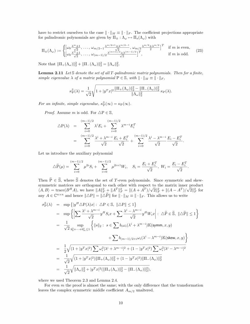
Lemma 2.11 Let S denote the set of all T -palindromic matrix polynomials. Then for a finite,simple eigenvalue ! of a matrix polynomial P " S, with % · %M * % · %F ,
#SP(!) =
1-2
;
1 + |yT x|2 %$+(#")%22 $ %$#(#")%22%#"%22
#P(!).
For an infinite, simple eigenvalue, #SP(() = #P(().
Proof. Assume m is odd. For &P " S,
&P(!) =(m#1)/2*
i=0
!iEi +(m#1)/2*
i=0
!m#iETi
=(m#1)/2*
i=0
!i + !m#i
-2
Ei + ETi-
2+
(m#1)/2*
i=0
!i $ !m#i
-2
Ei $ ETi-
2.
Let us introduce the auxiliary polynomial
&<P(µ) =(m#1)/2*
i=0
µ2iSi +(m#1)/2*
i=0
µ2i+1Wi, Si =Ei + ET
i-2
, Wi =Ei $ ET
i-2
.
Then <P " <S, where <S denotes the set of T -even polynomials. Since symmetric and skew-symmetric matrices are orthogonal to each other with respect to the matrix inner product4A, B5 = trace(BHA), we have %A%2F + %AT %2F = %(A + AT )/
-2%2F + %(A $ AT )/
-2%2F for
any A " Cn!n and hence %&P% = %&<P% for % · %M * % · %F . This allows us to write
)SP(!) = sup
(|yH&P(!)x| : &P " S, %&P% ) 1
)
= sup2++++
* !i + !m#i
-2
yHSix +* !i $ !m#i
-2
yHWix
++++ : &<P " <S, %&<P% ) 1=
=1-2
supb20+···+b2m(1
2%s%2 : s "
*bi"i(!i + !m#i)K(symm, x, y)
+*
b(m#1)/2+i"i(!i $ !m#i)K(skew, x, y)=
=12
1(1 + |yT x|2)
*"2
i |!i + !m#i|2 + (1$ |yT x|2)*
"2i |!i $ !m#i|2
=1-2
1(1 + |yT x|2)%$+(#")%22 + (1$ |yT x|2)%$#(#")%22
=1-2
1%#"%22 + |yT x|2(%$+(#")%22 $ %$#(#")%22),
where we used Theorem 2.3 and Lemma 2.4.For even m the proof is almost the same; with the only di"erence that the transformation
leaves the complex symmetric middle coe!cient Am/2 unaltered.
10
For ! = (, observe that the corresponding optimization problem (13) involves only asingle, unstructured coe!cient of the polynomial and hence palindromic structure has noe"ect on the condition number.
From the result of Lemma 2.11 it follows that a large di"erence between the structuredand unstructured condition numbers for T -palindromic matrix polynomials may occur when|yT x| is close to one, and %$+(#")%2 is close to zero. Assuming that all weights are positive,the latter condition implies that m is odd and and ! 3 $1. An instance of such a case isgiven by a variation of Example 2.8.
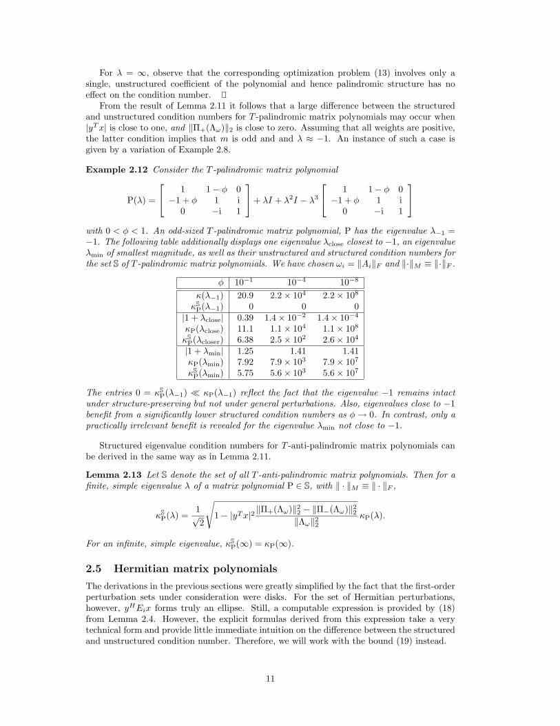
Example 2.12 Consider the T -palindromic matrix polynomial
P(!) =
7
81 1$ ( 0
$1 + ( 1 i0 $i 1
9
: + !I + !2I $ !3
7
81 1$ ( 0
$1 + ( 1 i0 $i 1
9
:
with 0 < ( < 1. An odd-sized T -palindromic matrix polynomial, P has the eigenvalue !#1 =$1. The following table additionally displays one eigenvalue !close closest to $1, an eigenvalue!min of smallest magnitude, as well as their unstructured and structured condition numbers forthe set S of T -palindromic matrix polynomials. We have chosen "i = %Ai%F and %·%M * %·%F .
( 10#1 10#4 10#8
#(!#1) 20.9 2.2! 104 2.2! 108
#SP(!#1) 0 0 0
|1 + !close| 0.39 1.4! 10#2 1.4! 10#4
#P(!close) 11.1 1.1! 104 1.1! 108
#SP(!closer) 6.38 2.5! 102 2.6! 104
|1 + !min| 1.25 1.41 1.41#P(!min) 7.92 7.9! 103 7.9! 107
#SP(!min) 5.75 5.6! 103 5.6! 107
The entries 0 = #SP(!#1) 1 #P(!#1) reflect the fact that the eigenvalue $1 remains intact
under structure-preserving but not under general perturbations. Also, eigenvalues close to $1benefit from a significantly lower structured condition numbers as ( / 0. In contrast, only apractically irrelevant benefit is revealed for the eigenvalue !min not close to $1.
Structured eigenvalue condition numbers for T -anti-palindromic matrix polynomials canbe derived in the same way as in Lemma 2.11.
Lemma 2.13 Let S denote the set of all T -anti-palindromic matrix polynomials. Then for afinite, simple eigenvalue ! of a matrix polynomial P " S, with % · %M * % · %F ,
#SP(!) =
1-2
;
1$ |yT x|2 %$+(#")%22 $ %$#(#")%22%#"%22
#P(!).
For an infinite, simple eigenvalue, #SP(() = #P(().
2.5 Hermitian matrix polynomials
The derivations in the previous sections were greatly simplified by the fact that the first-orderperturbation sets under consideration were disks. For the set of Hermitian perturbations,however, yHEix forms truly an ellipse. Still, a computable expression is provided by (18)from Lemma 2.4. However, the explicit formulas derived from this expression take a verytechnical form and provide little immediate intuition on the di"erence between the structuredand unstructured condition number. Therefore, we will work with the bound (19) instead.
11
Lemma 2.14 Let S denote the set of all Hermitian matrix polynomials. Then for a finite orinfinite, simple eigenvalue of a matrix polynomial P " S,
1.1
1$ 12 |yHx|2 #P(!) ) #S
P(!) ) #P(!) for % · %M * % · %2, and
2. #P(!)/-
2 ) #SP(!) ) #P(!) for % · %M * % · %F .
Proof. Let % · %M * % · %F . Then Theorem 2.3 states
K(Herm, x, y) ,= K(1/2, (yHx)2/2).
Consequently,"i!
iK(Herm, x, y) ,= K("2i |!|2i/2, "2
i !2i(yHx)2/2),
which implies
)SP(!) = sup
b20+···+b2m(1
2%s%2 : s "
m*
i=0
biK("2i !2i/2, "2
i !2i(yHx)2/2)=
.
By Lemma 2.4,1-2%#"%2 ) )S
P(!) ) %#"%2.
The proof for the case % · %M * % · %2 is analogous.
Remark 2.15 Since Hermitian and skew-Hermitian matrices are related by multiplicationwith i, which simply rotates the first-order perturbation set by 90 degrees, a slight modificationof the proof shows that the statement of Lemma 2.14 remains true when S denotes the spaceof H-odd or H-even polynomials. This can in turn be used – as in the proof of Lemma 2.11– to show that also for H-(anti-)palindromic polynomials there is at most an insignificantdi"erence between the structured and unstructured eigenvalue condition numbers.
3 Condition numbers for linearizations
As already mentioned in the introduction, polynomial eigenvalue problems are often solved byfirst linearizing the matrix polynomial into a larger matrix pencil. Of the classes of lineariza-tions proposed in the literature, the vector spaces DL(P) introduced in [28] are particularlyamenable to further analysis, while o"ering a degree of generality that is often su!cient inapplications.
Definition 3.1 Let #m#1 = [!m#1, !m#2 . . . !, 1]T and let P be a matrix polynomial ofdegree m. Then a matrix pencil L(!) = !X +Y " Cmn!mn is in DL(P) if there is a so calledansatz vector v " Cm satisfying
L(!) · (#m#1 0 I) = v 0 P (!) and (#Tm#1 0 I) · L(!) = vT 0 P (!).
It is easy to see that the ansatz vector v is uniquely determined by L " DL(P). In [28,Thm. 6.7] it has been shown that L " DL(P) is a linearization of P if and only if none of theeigenvalues of P is a root of the polynomial
p(µ; v) = v1µm#1 + v2µ
m#2 + · · · + vm#1µ + vm (24)
associated with the ansatz vector v. If P has eigenvalue (, this condition should be readas v1 '= 0. Apart from this elegant characterization, probably the most important propertyof DL(P) is that it leads to a simple one-to-one relation between the eigenvectors of P andL " DL(P). To keep the notation compact, we define #m#1 as in Definition 3.1 for finite !but let #m#1 = [1, 0, . . . , 0]T for ! = (.
12
Theorem 3.2 ([28]) Let P be a matrix polynomial and L " DL(P) with ansatz vector v.Then x '= 0 is a right eigenvector of P associated with an eigenvalue ! if and only if #m#10xis a right eigenvector of L associated with !. Similarly, y '= 0 is a left eigenvector of Passociated with an eigenvalue ! if and only if #m#1 0 y is a left eigenvector of L associatedwith !.
As a matrix pencil L(!) = !X + Y is a special case of a matrix polynomial, we can usethe results of Section 2 to study the (structured) eigenvalue condition numbers of L. Tosimplify the analysis, we will assume that the weights "0, . . . ,"m in the definition of %&P%are all equal to 1 for the rest of this paper. This assumption is only justified if P is notbadly scaled, i.e., the norms of the coe!cients of P do not vary significantly. To a certainextent, bad scaling can be overcome by rescaling the matrix polynomial before linearization,see [10, 14, 16, 17]. Moreover, we choose % · %v * % · %2 and assume that % · %M is an arbitrarybut fixed unitarily invariant matrix norm. The same norm is used for measuring perturbations&L(!) = &X + !&Y to the linearization L. To summarize
%&P% =1%E0%2M + %E1%M + · · · + %Em%2M , (25)
%&L% =1%&X%2M + %&Y %2M , (26)
for the rest of this paper. For unstructured eigenvalue condition numbers, Lemma 2.1 togetherwith Theorem 3.2 imply the following formula.
Lemma 3.3 Let ! be a finite, simple eigenvalue of a matrix polynomial P with normalizedright and left eigenvectors x and y. Then the eigenvalue condition number #L(!) for a lin-earization L " DL(P) with ansatz vector v satisfies
#L(!) =.
1 + |!|2|p(!; v)| · %#m#1%22
|yHP $(!)x| =.
1 + |!|2 %#m#1%22|p(!; v)| %#m%2
#P(!).
Proof. A similar formula for the case % · %v * % · %1 can be found in [16, Section 3]. Theproof for our case % · %v * % · %2 is almost identical and therefore omitted.
To allow for a simple interpretation of the result of Lemma 3.3, we define the quantity
*(!; v) :=%#m#1%2|p(!; v)| (27)
for a given ansatz vector v. Obviously *(!; v) 2 1. Since L is assumed to be a linearization,p(!; v) '= 0 and hence *(!; v) < (. Using the straightforward bound
1 ).
1 + |!|2%#m#1%2%#m%2
)-
2, (28)
the result of Lemma 3.3 yields
*(!; v) ) #L(!)#P(!)
)-
2 *(!; v). (29)
This shows that the process of linearizing P invariably increases the condition number of asimple eigenvalue of P at least by a factor of *(!; v) and at most by a factor of
-2*(!; v). In
other words, *(!; v) serves as a growth factor for the eigenvalue condition number.Since p(!; v) = #T
m#1v, it follows from the Cauchy-Schwartz inequality that among allansatz vectors with %v%2 = 1 the vector v = #m#1/%#m#1%2 minimizes *(!; v) and, hence,for this particular choice of v we have *(!; v) = 1 and
#P(!) ) #L(!) )-
2 #P(!).
13
Let us emphasize that this result is primarily of theoretical interest as the optimal choiceof v depends on the (typically unknown) eigenvalue !. A practically more useful recipe isto choose v = [1, 0, . . . , 0]T if |!| 2 1 and v = [0, . . . , 0, 1]T if |!| ) 1. In both cases,*(!; v) = '"m$1'2
|p(#;v)| )-
m and therefore #P(!) ) #L(!) )-
2m #P(!).In the following section, the discussion above shall be extended to structured linearizations
and condition numbers.
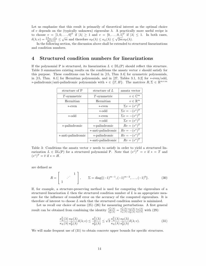
4 Structured condition numbers for linearizations
If the polynomial P is structured, its linearization L " DL(P) should reflect this structure.Table 3 summarizes existing results on the conditions the ansatz vector v should satisfy forthis purpose. These conditions can be found in [15, Thm 3.4] for symmetric polynomials,in [15, Thm. 6.1] for Hermitian polynomials, and in [27, Tables 3.1, 3.2] for #-even/odd,#-palindromic/anti-palindromic polynomials with # " {T, H}. The matrices R,% " Rm!m
structure of P structure of L ansatz vector
T -symmetric T -symmetric v " Cm
Hermitian Hermitian v " Rm
#-even #-even %v = (v")T
#-odd %v = $(v")T
#-odd #-even %v = $(v")T
#-odd %v = (v")T
#-palindromic #-palindromic Rv = (v")T
#-anti-palindromic Rv = $(v")T
#-anti-palindromic #-palindromic Rv = $(v")T
#-anti-palindromic Rv = (v")T
Table 3: Conditions the ansatz vector v needs to satisfy in order to yield a structured lin-earization L " DL(P) for a structured polynomial P. Note that (v")T = v if # = T and(v")T = v if # = H.
are defined as
R =
7
81
. . .
1
9
: , % = diag{($1)m#1, ($1)m#2, . . . , ($1)0}. (30)
If, for example, a structure-preserving method is used for computing the eigenvalues of astructured linearization L then the structured condition number of L is an appropriate mea-sure for the influence of roundo" error on the accuracy of the computed eigenvalues. It istherefore of interest to choose L such that the structured condition number is minimized.
Let us recall our choice of norms (25)–(26) for measuring perturbations. A first generalresult can be obtained from combining the identity $S
L(#)$SP(#)
= $SL(#)
$L(#)$P(#)$SP(#)
$L(#)$P(#) with (29):
#SL(!)
#L(!)#P(!)#S
P(!)*(!; v) ) #S
L(!)#S
P(!))-
2#S
L(!)#L(!)
#P(!)#S
P(!)*(!; v). (31)
We will make frequent use of (31) to obtain concrete upper bounds for specific structures.
14
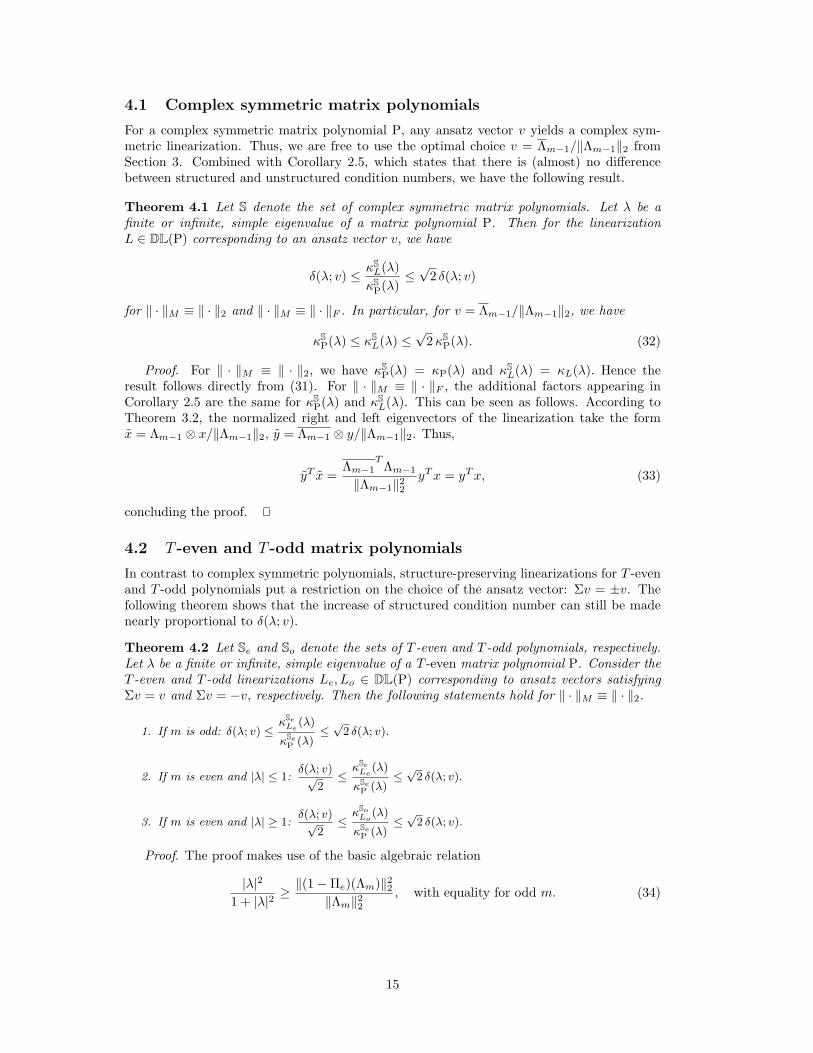
4.1 Complex symmetric matrix polynomials
For a complex symmetric matrix polynomial P, any ansatz vector v yields a complex sym-metric linearization. Thus, we are free to use the optimal choice v = #m#1/%#m#1%2 fromSection 3. Combined with Corollary 2.5, which states that there is (almost) no di"erencebetween structured and unstructured condition numbers, we have the following result.
Theorem 4.1 Let S denote the set of complex symmetric matrix polynomials. Let ! be afinite or infinite, simple eigenvalue of a matrix polynomial P. Then for the linearizationL " DL(P) corresponding to an ansatz vector v, we have
*(!; v) ) #SL(!)
#SP(!)
)-
2 *(!; v)
for % · %M * % · %2 and % · %M * % · %F . In particular, for v = #m#1/%#m#1%2, we have
#SP(!) ) #S
L(!) )-
2 #SP(!). (32)
Proof. For % · %M * % · %2, we have #SP(!) = #P(!) and #S
L(!) = #L(!). Hence theresult follows directly from (31). For % · %M * % · %F , the additional factors appearing inCorollary 2.5 are the same for #S
P(!) and #SL(!). This can be seen as follows. According to
Theorem 3.2, the normalized right and left eigenvectors of the linearization take the formx = #m#1 0 x/%#m#1%2, y = #m#1 0 y/%#m#1%2. Thus,
yT x =#m#1
T #m#1
%#m#1%22yT x = yT x, (33)
concluding the proof.
4.2 T -even and T -odd matrix polynomials
In contrast to complex symmetric polynomials, structure-preserving linearizations for T -evenand T -odd polynomials put a restriction on the choice of the ansatz vector: %v = ±v. Thefollowing theorem shows that the increase of structured condition number can still be madenearly proportional to *(!; v).
Theorem 4.2 Let Se and So denote the sets of T -even and T -odd polynomials, respectively.Let ! be a finite or infinite, simple eigenvalue of a T -even matrix polynomial P. Consider theT -even and T -odd linearizations Le, Lo " DL(P) corresponding to ansatz vectors satisfying%v = v and %v = $v, respectively. Then the following statements hold for % · %M * % · %2.
1. If m is odd: !("; v) !#Se
Le(")
#SeP (")
!"
2 !("; v).
2. If m is even and |"| ! 1:!("; v)"
2!
#SeLe
(")
#SeP (")
!"
2 !("; v).
3. If m is even and |"| # 1:!("; v)"
2!
#SoLo
(")
#SeP (")
!"
2 !("; v).
Proof. The proof makes use of the basic algebraic relation
|!|2
1 + |!|2 2%(1$$e)(#m)%22
%#m%22, with equality for odd m. (34)
15
1. If m is odd, (34) implies – together with Lemma 2.6 and (33) – the equality
#SeLe
(!)#Se
P (!)=
11$ |yT x|2 |#|2
1+|#|211$ |yT x|2 '(1#!e)("m)'22
'"m'22
· #Le(!)#P(!)
=#Le(!)#P(!)
. (35)
Now the desired result follows directly from our general bounds (31).
2. If m is even and |!| ) 1 then
1-2· #Le(!)
#P(!))
#SeLe
(!)#Se
P (!)) #Le(!)
#P(!),
where the lower and upper bounds follow from the first equality in (35) using |#|21+|#|2 )
12
and (34), respectively. Again, the desired result follows from (31).
3. If m is even, |!| 2 1 and a T -odd linearization is used then Lemma 2.10 along with (33)yield
#SoLo
(!)#Se
P (!)=
11$ |yT x|2 1
1+|#|21
1$ |yT x|2 '(1#!e)("m)'22'"m'22
· #Lo(!)#P(!)
.
The relation%(1$$e)(#m)%22
%#m%22) 1
1 + |!|2 )12
then implies1-2· #Lo(!)
#P(!))
#SoLo
(!)#Se
P (!)) #Lo(!)
#P(!).
Hence the result follows from (31).
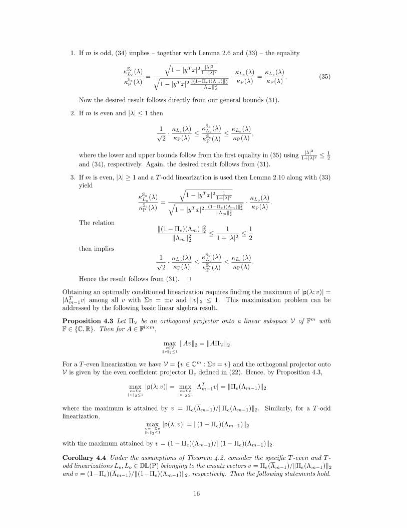
Obtaining an optimally conditioned linearization requires finding the maximum of |p(!; v)| =|#T
m#1v| among all v with %v = ±v and %v%2 ) 1. This maximization problem can beaddressed by the following basic linear algebra result.
Proposition 4.3 Let $V be an orthogonal projector onto a linear subspace V of Fm withF " {C, R}. Then for A " Fl!m,
maxv!V
#v#2"1
%Av%2 = %A$V%2.
For a T -even linearization we have V = {v " Cm : %v = v} and the orthogonal projector ontoV is given by the even coe!cient projector $e defined in (22). Hence, by Proposition 4.3,
maxv=!v#v#2"1
|p(!; v)| = maxv=!v#v#2"1
|#Tm#1v| = %$e(#m#1)%2
where the maximum is attained by v = $e(#m#1)/%$e(#m#1)%2. Similarly, for a T -oddlinearization,
maxv=$!v#v#2"1
|p(!; v)| = %(1$$e)(#m#1)%2
with the maximum attained by v = (1$$e)(#m#1)/%(1$$e)(#m#1)%2.
Corollary 4.4 Under the assumptions of Theorem 4.2, consider the specific T -even and T -odd linearizations Le, Lo " DL(P) belonging to the ansatz vectors v = $e(#m#1)/%$e(#m#1)%2and v = (1$$e)(#m#1)/%(1$$e)(#m#1)%2, respectively. Then the following statements hold.
16
1. If m is odd: #SeP (!) ) #Se
Le(!) ) 2 #Se
P (!).
2. If m is even and |!| ) 1: #SeP (!)/
-2 ) #Se
Le(!) ) 2 #Se
P (!).
3. If m is even and |!| 2 1: #SeP (!)/
-2 ) #So
Lo(!) ) 2 #Se
P (!).
Proof. Note that, by definition, *(!; v) 2 1 and hence all lower bounds are direct conse-quences of Theorem 4.2. To show *(!; v) )
-2 for the upper bounds of statements 1 and 2,
we make use of the inequalities
%$e(#m#1)% ) %#m#1%2 )-
2%$e(#m#1)%, (36)
which hold if either m is odd or m is even and |!| ) 1. For statement 3, the bound *(!; v) )-
2is a consequence of (34).
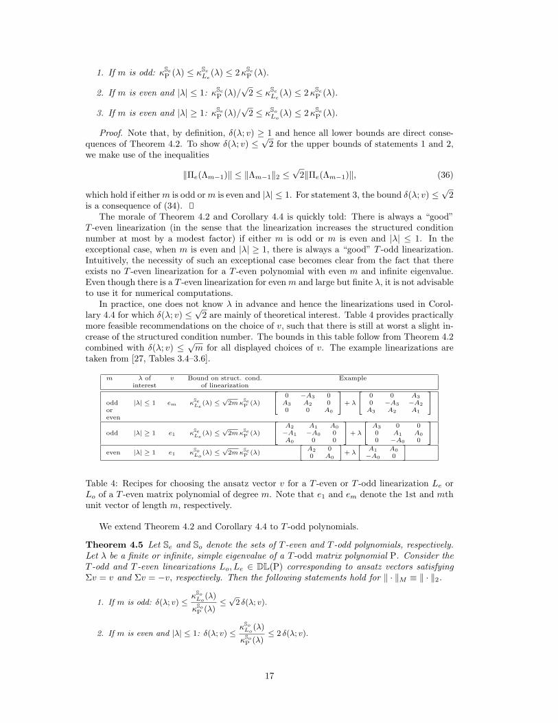
The morale of Theorem 4.2 and Corollary 4.4 is quickly told: There is always a “good”T -even linearization (in the sense that the linearization increases the structured conditionnumber at most by a modest factor) if either m is odd or m is even and |!| ) 1. In theexceptional case, when m is even and |!| 2 1, there is always a “good” T -odd linearization.Intuitively, the necessity of such an exceptional case becomes clear from the fact that thereexists no T -even linearization for a T -even polynomial with even m and infinite eigenvalue.Even though there is a T -even linearization for even m and large but finite !, it is not advisableto use it for numerical computations.
In practice, one does not know ! in advance and hence the linearizations used in Corol-lary 4.4 for which *(!; v) )
-2 are mainly of theoretical interest. Table 4 provides practically
more feasible recommendations on the choice of v, such that there is still at worst a slight in-crease of the structured condition number. The bounds in this table follow from Theorem 4.2combined with *(!; v) )
-m for all displayed choices of v. The example linearizations are
taken from [27, Tables 3.4–3.6].
m # of v Bound on struct. cond. Exampleinterest of linearization
oddoreven
|#| ( 1 em $SeLe
(#) (*
2m $SeP (#)
2
40 #A3 0
A3 A2 00 0 A0
3
5 + #
2
40 0 A30 #A3 #A2
A3 A2 A1
3
5
odd |#| + 1 e1 $SeLe
(#) (*
2m $SeP (#)
2
4A2 A1 A0#A1 #A0 0A0 0 0
3
5 + #
2
4A3 0 00 A1 A00 #A0 0
3
5
even |#| + 1 e1 $SoLo
(#) (*
2m $SeP (#)
»A2 00 A0
–+ #
»A1 A0#A0 0
–
Table 4: Recipes for choosing the ansatz vector v for a T -even or T -odd linearization Le orLo of a T -even matrix polynomial of degree m. Note that e1 and em denote the 1st and mthunit vector of length m, respectively.
We extend Theorem 4.2 and Corollary 4.4 to T -odd polynomials.
Theorem 4.5 Let Se and So denote the sets of T -even and T -odd polynomials, respectively.Let ! be a finite or infinite, simple eigenvalue of a T -odd matrix polynomial P. Consider theT -odd and T -even linearizations Lo, Le " DL(P) corresponding to ansatz vectors satisfying%v = v and %v = $v, respectively. Then the following statements hold for % · %M * % · %2.
1. If m is odd: !("; v) !#So
Lo(")
#SoP (")
!"
2 !("; v).
2. If m is even and |"| ! 1: !("; v) !#So
Lo(")
#SoP (")
! 2 !("; v).
17
3. If m is even and |"| # 1: !("; v) !#Se
Le(")
#SoP (")
! 2 !("; v).
Proof.
1. Similar to the proof of Theorem 4.2, Lemma 2.10 yields
#SoLo
(!)#So
P (!)=
11$ |yT x|2 1
1+|#|21
1$ |yT x|2 '!e("m)'22'"m'22
· #Lo(!)#P(!)
. (37)
Relation (34) implies 1/(1 + |!|2) = %$e(#m)%22/%#m%22 and hence$So
Lo(#)
$SoP (#)
= $Lo (#)$P(#) ,
which proves the first statement by (31).
2. If m is even and |!| ) 1, relation (34) yields 1/(1+ |!|2) ) %$e(#m)%22/%#m%22, implying
1 )
11$ |yT x|2 1
1+|#|21
1$ |yT x|2 '!e("m)'22'"m'22
)
11$ 1
1+|#|21
1$ '!e("m)'22'"m'22
=%#m%2%#m#1%2
).
1 + |!|2 )-
2,
where the previous last bound follows from (28). Combined with (37) and (31), thisshows the bounds of the second statement.
3. For m even and |!| 2 1, a T -even linearization gives
#SeLe
(!)#So
P (!)=
11$ |yT x|2 |#|2
1+|#|211$ |yT x|2 '!e("m)'22
'"m'22
· #Le(!)#P(!)
.
It is not hard to verify |#|21+|#|2 )
'!e("m)'22'"m'22
, implying
1 )
11$ |yT x|2 |#|2
1+|#|211$ |yT x|2 '!e("m)'22
'"m'22
)
11$ |#|2
1+|#|211$ '!e("m)'22
'"m'22
=%#m%2
|!| · %#m#1%2)
.1 + |!|2|!| )
-2,
where the previous last bound follows again from (28). This concludes the proof by (31).
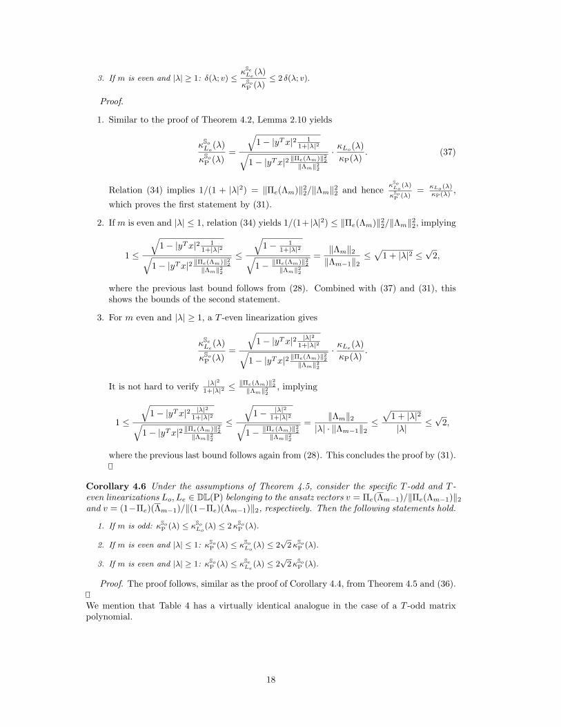
Corollary 4.6 Under the assumptions of Theorem 4.5, consider the specific T -odd and T -even linearizations Lo, Le " DL(P) belonging to the ansatz vectors v = $e(#m#1)/%$e(#m#1)%2and v = (1$$e)(#m#1)/%(1$$e)(#m#1)%2, respectively. Then the following statements hold.
1. If m is odd: #SoP (") ! #So
Lo(") ! 2 #So
P (").
2. If m is even and |"| ! 1: #SoP (") ! #So
Lo(") ! 2
"2 #So
P (").
3. If m is even and |"| # 1: #SoP (") ! #Se
Le(") ! 2
"2 #So
P (").
Proof. The proof follows, similar as the proof of Corollary 4.4, from Theorem 4.5 and (36).
We mention that Table 4 has a virtually identical analogue in the case of a T -odd matrixpolynomial.
18
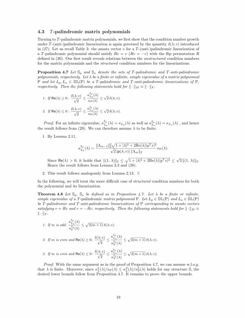
4.3 T -palindromic matrix polynomials
Turning to T -palindromic matrix polynomials, we first show that the condition number growthunder T -(anti-)palindromic linearization is again governed by the quantity *(!; v) introducedin (27). Let us recall Table 3: the ansatz vector v for a T -(anti-)palindromic linearization ofa T -palindromic polynomial should satisfy Rv = v (Rv = $v) with the flip permutation Rdefined in (30). Our first result reveals relations between the unstructured condition numbersfor the matrix polynomials and the structured condition numbers for the linearizations.
Proposition 4.7 Let Sp and Sa denote the sets of T -palindromic and T -anti-palindromicpolynomials, respectively. Let ! be a finite or infinite, simple eigenvalue of a matrix polynomialP and let Lp, La " DL(P) be a T -palindromic and T -anti-palindromic linearizations of P,respectively. Then the following statements hold for % · %M * % · %F .
1. If Re(") # 0 :!("; v)"
2!
#SpLp
(")
#P(")!"
2 !("; v).
2. If Re(") ! 0 :!("; v)"
2!
#SaLa
(")
#P(")!"
2 !("; v).
Proof. For an infinite eigenvalue, #Sp
Lp(!) = #Lp(!) as well as #Sa
La(!) = #La(!) , and hence
the result follows from (29). We can therefore assume ! to be finite.
1. By Lemma 2.11,
#Sp
Lp(!) =
%#m#1%22.
1 + |!|2 + 2Re(!)|yT x|2-2 |p(!; v)| %#m%2
#P(!).
Since Re(!) > 0, it holds that %(1, !)%2 ).
1 + |!|2 + 2Re(!)|yT x|2 )-
2 %(1, !)%2.Hence the result follows from Lemma 3.3 and (28).
2. This result follows analogously from Lemma 2.13.
In the following, we will treat the more di!cult case of structured condition numbers for boththe polynomial and its linearization.
Theorem 4.8 Let Sp, Sa be defined as in Proposition 4.7. Let ! be a finite or infinite,simple eigenvalue of a T -palindromic matrix polynomial P. Let Lp " DL(P) and La " DL(P)be T -palindromic and T -anti-palindromic linearizations of P corresponding to ansatz vectorssatisfying v = Rv and v = $Rv, respectively. Then the following statements hold for % ·%M *% · %F .
1. If m is odd:#
SpLp
(")
#SpP (")
!p
2(m + 1) !("; v).
2. If m is even and Re(") # 0:!("; v)"
2!
#SpLp
(")
#SpP (")
!p
2(m + 1) !("; v).
3. If m is even and Re(") ! 0:!("; v)"
2!
#SaLa
(")
#SpP (")
!p
2(m + 1) !("; v).
Proof. With the same argument as in the proof of Proposition 4.7, we can assume w.l.o.g.that ! is finite. Moreover, since #S
L(!)/#P(!) ) #SL(!)/#S
P(!) holds for any structure S, thedesired lower bounds follow from Proposition 4.7. It remains to prove the upper bounds.
19
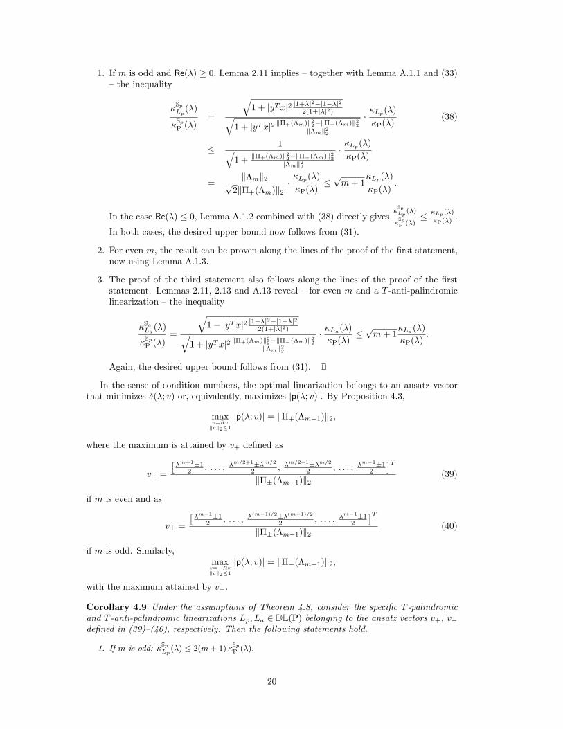
1. If m is odd and Re(!) 2 0, Lemma 2.11 implies – together with Lemma A.1.1 and (33)– the inequality
#Sp
Lp(!)
#Sp
P (!)=
11 + |yT x|2 |1+#|2#|1##|2
2(1+|#|2)11 + |yT x|2 '!+("m)'22#'!$("m)'22
'"m'22
·#Lp(!)#P(!)
(38)
) 111 + '!+("m)'22#'!$("m)'22
'"m'22
·#Lp(!)#P(!)
=%#m%2-
2%$+(#m)%2·#Lp(!)#P(!)
)-
m + 1#Lp(!)#P(!)
.
In the case Re(!) ) 0, Lemma A.1.2 combined with (38) directly gives$
SpLp
(#)
$SpP (#)
) $Lp (#)
$P(#) .
In both cases, the desired upper bound now follows from (31).
2. For even m, the result can be proven along the lines of the proof of the first statement,now using Lemma A.1.3.
3. The proof of the third statement also follows along the lines of the proof of the firststatement. Lemmas 2.11, 2.13 and A.13 reveal – for even m and a T -anti-palindromiclinearization – the inequality
#SaLa
(!)
#Sp
P (!)=
11$ |yT x|2 |1##|2#|1+#|2
2(1+|#|2)11 + |yT x|2 '!+("m)'22#'!$("m)'22
'"m'22
· #La(!)#P(!)
)-
m + 1#La(!)#P(!)
.
Again, the desired upper bound follows from (31).
In the sense of condition numbers, the optimal linearization belongs to an ansatz vectorthat minimizes *(!; v) or, equivalently, maximizes |p(!; v)|. By Proposition 4.3,
maxv=Rv#v#2"1
|p(!; v)| = %$+(#m#1)%2,
where the maximum is attained by v+ defined as
v± =/
#m$1±12 , . . . , #m/2+1±#m/2
2 , #m/2+1±#m/2
2 , . . . , #m$1±12
0T
%$±(#m#1)%2(39)
if m is even and as
v± =/
#m$1±12 , . . . , #(m$1)/2±#(m$1)/2
2 , . . . , #m$1±12
0T
%$±(#m#1)%2(40)
if m is odd. Similarly,max
v=$Rv#v#2"1
|p(!; v)| = %$#(#m#1)%2,
with the maximum attained by v#.
Corollary 4.9 Under the assumptions of Theorem 4.8, consider the specific T -palindromicand T -anti-palindromic linearizations Lp, La " DL(P) belonging to the ansatz vectors v+, v#defined in (39)–(40), respectively. Then the following statements hold.
1. If m is odd: #SpLp
(") ! 2(m + 1) #SpP (").
20
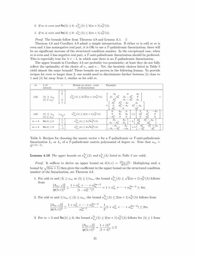
2. If m is even and Re(") # 0: #SpLp
(") ! 2(m + 1) #SpP (").
3. If m is even and Re(") ! 0: #SaLa
(") ! 2(m + 1) #SpP (").
Proof. The bounds follow from Theorem 4.8 and Lemma A.1.Theorem 4.8 and Corollary 4.9 admit a simple interpretation. If either m is odd or m is
even and ! has nonnegative real part, it is OK to use a T -palindromic linearization; there willbe no significant increase of the structured condition number. In the exceptional case, whenm is even and ! has negative real part, a T -anti-palindromic linearization should be preferred.This is especially true for ! = $1, in which case there is no T -palindromic linearization.
The upper bounds in Corollary 4.8 are probably too pessimistic; at least they do not fullyreflect the optimality of the choice of v+ and v#. Yet, the heuristic choices listed in Table 5yield almost the same bounds! These bounds are proven in the following lemma. To providerecipes for even m larger than 2, one would need to discriminate further between |!| close to1 and |!| far away from 1, similar as for odd m.
m # of v Bound on struct. cond. Exampleinterest of linearization
odd |#| + %m
|#| ( %$1m
2
66664
10...01
3
77775$
SpLp
(#) ( 2*
2(m + 1)$SpP (#)
2
4A0 0 A0
A1 # AT0 A0 # AT
1 0AT
1 A1 # AT0 A0
3
5 +
#
2
4AT
0 AT1 # A0 A1
0 AT0 # A1 AT
1 # A0AT
0 0 AT0
3
5
odd |#| ( %m
|#| + %$1m
e m$12
$SpLp
(#) ( 2(m + 1)$SpP (#)
2
40 A0 00 A1 A0
#AT0 0 0
3
5+#
2
40 0 #A0
AT0 AT
1 00 AT
0 0
3
5
m = 2 Re(#) + 0
»11
–$
SpLp
(#) ( 2*
3$SpP (#)
»A0 A0
A1 # AT0 A0
–+ #
»AT
0 AT1 # A0
AT0 AT
0
–
m = 2 Re(#) ( 0
»1#1
–$Sa
La(#) ( 2
*3$
SpP (#)
»#A0 A0
#A1 # AT0 #A0
–+#
»AT
0 AT1 + A0
#AT0 AT
0
–
Table 5: Recipes for choosing the ansatz vector v for a T -palindromic or T -anti-palindromiclinearization Le or Lo of a T -palindromic matrix polynomial of degree m. Note that %m =21/(m#1).
Lemma 4.10 The upper bounds on #Sp
Lp(!) and #Sa
La(!) listed in Table 5 are valid.
Proof. It su!ces to derive an upper bound on *(!; v) = '"m$1'2p(#;v) . Multiplying such a
bound by.
2(m + 1) then gives the coe!cient in the upper bound on the structured conditionnumber of the linearization, see Theorem 4.8.
1. For odd m and |!| 2 %m or |!| ) 1/%m, the bound #Sp
Lp(!) )
-2(m + 1)#
Sp
P (!) followsfrom
%#m#1%22|p(!; v)|2 )
1 + %2m + · · · + %2m#2
m
|1$ %m#1m |2
= 1 + %2m + · · · + %2m#2
m ) 4m.
2. For odd m and 1/%m ) |!| ) %m, the bound #Sp
Lp(!) ) 2(m + 1) #
Sp
P (!) follows from
%#m#1%22|p(!; v)|2 )
1 + %2m + · · · + %2m#2
m
%m#1m
=12(1 + %2
m + · · · + %2m#2m ) ) 2m.
3. For m = 2 and Re(!) 2 0, the bound #Sp
Lp(!) ) 2(m + 1)#
Sp
P (!) follows for |!| ) 1 from
%#m#1%22|p(!; v)|2 =
1 + |!|2
|1 + !|2 ) 2
21
and for |!| 2 1 from%#m#1%22|p(!; v)|2 =
|!|2
|!|21
|#|2 + 1
| 1# + 1|2) 2.
4. The proof for m = 2 and Re(!) ) 0 is analogous to Part 3.
For T -anti-palindromic polynomials, the implications of Theorems 4.8 and 4.7, Corol-lary 4.9 and Table 5 hold, but with the roles of T -palindromic and T -anti-palindromic ex-changed. For example, if either m is odd or m is even and Re(!) 2 0, there is always agood T -anti-palindromic linearization. Otherwise, if m is even and Re(!) ) 0, there is a goodT -palindromic linearization.
4.4 Hermitian matrix polynomials and related structures
The linearization of a Hermitian polynomial is also Hermitian if the corresponding ansatzvector v is real, see Table 3. The optimal v, which maximizes |p(!; v)|, could be found byfinding the maximal singular value and the corresponding left singular vector of the real m!2matrix [Re(#m#1), Im(#m#1)]. Instead of invoking the rather complicated expression for thisoptimal choice, the following lemma uses a heuristic choice of v.
Lemma 4.11 Let Sh denote the set of Hermitian polynomials. Let ! be a finite or infinite,simple eigenvalue of a Hermitian matrix polynomial P. Then the following statements holdfor % · %M * % · %F .
1. If |!| 2 1 then the linearization L corresponding to the ansatz vector v = [1, 0, . . . , 0] isHermitian and satisfies #Sh
L (!) ) 2-
m#ShP (!).
2. If |!| ) 1 then the linearization L corresponding to the ansatz vector v = [0, . . . , 0, 1] isHermitian and satisfies #Sh
L (!) ) 2-
m#ShP (!).
Proof. Assume |!| 2 1. Lemma 2.14 together with Lemma 3.3 and (28) imply
#ShL (!)
#ShP (!)
)-
2#Lp(!)#P(!)
=-
2%#m#1%2|p(!; v)| ) 2
-m|!|m
|!|m = 2-
m.
The proof for |!| ) 1 proceeds analogously.H-even and H-odd matrix polynomials are closely related to Hermitian matrix polyno-
mials, see Remark 2.15. In particular, Lemma 4.11 applies verbatim to H-even and H-oddpolynomials. Note, however, that in the case of even m the ansatz vector v = [1, 0, . . . , 0]yields an H-odd linearization for an H-even polynomial, and vice versa. Similarly, the recipesof Table 5 can be extended to H-palindromic polynomials.
5 Summary and conclusions
We have derived relatively simple expressions for the structured eigenvalue condition numbersof certain structured matrix polynomials. These expressions have been used to analyze thepossible increase of the condition numbers when the polynomial is replaced by a structuredlinearization. At least in the case when all coe!cients of the polynomial are perturbed tothe same extent, the result is very positive: There is always a structured linearization, whichdepends on the eigenvalue of interest, such that the condition numbers increase at most by afactor linearly depending on m. We have also provided recipes for structured linearizations,which do not depend on the exact value of the eigenvalue, and for which the increase ofthe condition number is still negligible. Hence, the accuracy of a strongly backward stableeigensolver applied to the structured linearization will fully enjoy the benefits of structure onthe sensitivity of an eigenvalue for the original matrix polynomial. The techniques and proofsof this paper represent yet another testimonial for the versatility of the linearization spacesintroduced by Mackey, Mackey, Mehl, and Mehrmann in [27, 28].
22
6 Acknowledgments
The authors thank Shreemayee Bora for inspiring discussions on the subject of this paper.Parts of this work was performed while the first author was staying at ETH Zurich. Thefinancial support by the Indo Swiss Bilateral Research Initiative (ISBRI), which made thisvisit possible, is gratefully acknowledged.
References
[1] S. S. Ahmad. Pseudospectra of Matrix Pencils and Their Applications in PeturbationAnalysis of Eigenvalues and Eigendecompositions. PhD thesis, Department of Mathe-matics, IIT Guhawati, India, 2007.
[2] S. S. Ahmad and R. Alam. Pseudospectra, critical points and multiple eigenvalues ofmatrix polynomials. Linear Algebra Appl., 430:1171–1195, 2009.
[3] A. L. Andrew, E. K.-W. Chu, and P. Lancaster. Derivatives of eigenvalues and eigenvec-tors of matrix functions. SIAM J. Matrix Anal. Appl., 14(4):903–926, 1993.
[4] F. S. V. Bazan. Eigenvalues of Matrix Polynomials, Sensitivity, Computation and Ap-plications (in Portuguese). IMPA, Rio de Janeiro, Brazil, 2003.
[5] M. Berhanu. The Polynomial Eigenvalue Problem. PhD thesis, School of Mathematics,The University of Manchester, UK, 2005.
[6] S. Bora. Structured eigenvalue condition number and backward error of a class of polyno-mial eigenvalue problems. Preprint 31-2006, Institut fur Mathematik, TU Berlin, 2006.
[7] R. Byers and D. Kressner. On the condition of a complex eigenvalue under real pertur-bations. BIT, 44(2):209–215, 2004.
[8] E. K.-W. Chu. Perturbation of eigenvalues for matrix polynomials via the Bauer-Fiketheorems. SIAM J. Matrix Anal. Appl., 25(2):551–573, 2003.
[9] J.-P. Dedieu and F. Tisseur. Perturbation theory for homogeneous polynomial eigenvalueproblems. Linear Algebra Appl., 358:71–94, 2003.
[10] H.-Y. Fan, W.-W. Lin, and P. Van Dooren. Normwise scaling of second order polynomialmatrices. SIAM J. Matrix Anal. Appl., 26(1):252–256, 2004.
[11] G. H. Golub and C. F. Van Loan. Matrix Computations. Johns Hopkins University Press,Baltimore, MD, third edition, 1996.
[12] D. J. Higham and N. J. Higham. Structured backward error and condition of generalizedeigenvalue problems. SIAM J. Matrix Anal. Appl., 20(2):493–512, 1999.
[13] N. J. Higham. Accuracy and Stability of Numerical Algorithms. SIAM, Philadelphia, PA,second edition, 2002.
[14] N. J. Higham, R.-C. Li, and F. Tisseur. Backward error of polynomial eigenproblemssolved by linearization. SIAM J. Matrix Anal. Appl., 29(4):1218–1241, 2007.
[15] N. J. Higham, D. S. Mackey, N. Mackey, and F. Tisseur. Symmetric linearizations formatrix polynomials. SIAM J. Matrix Anal. Appl., 29(1):143–159, 2007.
[16] N. J. Higham, D. S. Mackey, and F. Tisseur. The conditioning of linearizations of matrixpolynomials. SIAM J. Matrix Anal. Appl., 28(4):1005–1028, 2006.
23
[17] N. J. Higham, D. S. Mackey, F. Tisseur, and S. D. Garvey. Scaling, sensitivity andstability in the numerical solution of quadratic eigenvalue problems. Internat. J. Numer.Methods Engrg., 73(3):344–360, 2008.
[18] A. Hilliges, C. Mehl, and V. Mehrmann. On the solution of palindromic eigenvalueproblems. In Proceedings of ECCOMAS, Jyvaskyla, Finland, 2004.
[19] M. Karow. µ-values and spectral value sets for linear perturbation classes defined by ascalar product, 2007. Submitted.
[20] M. Karow. Structured pseudospectra and the condition of a nonderogatory eigenvalue,2007. Submitted.
[21] M. Karow, D. Kressner, and F. Tisseur. Structured eigenvalue condition numbers. SIAMJ. Matrix Anal. Appl., 28(4):1052–1068, 2006.
[22] D. Kressner, M. J. Pelaez, and J. Moro. Structured Holder condition numbers for multipleeigenvalues. Uminf report, Department of Computing Science, Umea University, Sweden,October 2006. Revised January 2008.
[23] A. Kurzhanski and I. Valyi. Ellipsoidal calculus for estimation and control. Systems &Control: Foundations & Applications. Birkhauser Boston Inc., Boston, MA, 1997.
[24] P. Lancaster, A. S. Markus, and F. Zhou. Perturbation theory for analytic matrix func-tions: the semisimple case. SIAM J. Matrix Anal. Appl., 25(3):606–626, 2003.
[25] H. Langer and B. Najman. Remarks on the perturbation of analytic matrix functions.II. Integral Equations Operator Theory, 12(3):392–407, 1989.
[26] H. Langer and B. Najman. Leading coe!cients of the eigenvalues of perturbed analyticmatrix functions. Integral Equations Operator Theory, 16(4):600–604, 1993.
[27] D. S. Mackey, N. Mackey, C. Mehl, and V. Mehrmann. Structured polynomial eigen-value problems: good vibrations from good linearizations. SIAM J. Matrix Anal. Appl.,28(4):1029–1051, 2006.
[28] D. S. Mackey, N. Mackey, C. Mehl, and V. Mehrmann. Vector spaces of linearizationsfor matrix polynomials. SIAM J. Matrix Anal. Appl., 28(4):971–1004, 2006.
[29] V. Mehrmann and H. Xu. Perturbation of purely imaginary eigenvalues of hamiltonianmatrices under structured perturbations. Electron. J. Linear Algebra, 17:234–257, 2008.
[30] S. Noschese and L. Pasquini. Eigenvalue condition numbers: zero-structured versustraditional. J. Comput. Appl. Math., 185(1):174–189, 2006.
[31] S. M. Rump. Eigenvalues, pseudospectrum and structured perturbations. Linear AlgebraAppl., 413(2-3):567–593, 2006.
[32] G. W. Stewart and J.-G. Sun. Matrix Perturbation Theory. Academic Press, New York,1990.
[33] F. Tisseur. Backward error and condition of polynomial eigenvalue problems. LinearAlgebra Appl., 309(1-3):339–361, 2000.
24
A Appendix
The following lemma summarizes some auxiliary results needed in the proofs of Section 4.3.
Lemma A.1 Let ! " C and let #± be defined as in (23. Then the following statements hold.
1. Assume m is odd. If Re(!) 2 0 then '!+("m)'22'"m'22
2 12(m+1) . If Re(!) ) 0 then
'!$("m)'22'"m'22
2 12(m+1) .
2. Assume m is odd. If Re(!) ) 0 then '!+("m)'22#'!$("m)'22'"m'22
2 |1+#|2#|1##|22(1+|#|2) .
3. Assume m is even. Then '!+("m)'22'"m'22
2 12(m+1) .
Proof.
1. For |!| 2 1 the statement follows from %#m%22 ) (m + 1)|!|2m and
2%$+(#m)%22 2 |!m + 1|2 + |!(m+1)/2 + !(m#1)/2|2
= |!|2m + 2Re(!m) + 1 + |!|m#1(|!|2 + Re(!) + 1)2 |!|2m $ 2|!|m + 1 + |!|m#1(|!|2 + 1)= |!|2m + 1 + |!|m#1(|!|$ 1)2 2 |!|2m.
If |!| ) 1, we can apply an analogous argument with ! replaced by 1/! to
%$+(#m)%22%#m%22
=|!|2m
|!|2m·
>
?(m#1)/2*
k=0
12
++++1!k
+1
!m#k
++++2@
AB C
m*
k=0
1|!|2k
D.
The second part follows from the first part by the substitution ! / $!.
2. Using (1 + |!|2)(1 + |!|4 + · · ·+ |!|(2m#2)) = %#m%22, we prove the equivalent statement
%$+(#m)%22 2 (|1 + !|2 $ |1$ !|2)(1 + |!|4 + · · · + |!|(2m#2)).
Assume |!| ) 1. Then the statement follows if we can show
%$+(#m)%22 $ %$#(#m)%22 214(|1 + !|2 $ |1$ !|2)(m + 1). (41)
Inserting ! = |!|(cos(() + i sin(()), we expand
%$+(#m)%22 $ %$#(#m)%22 =12
(m#1)/2*
k=0
|!m#k + !k|2 $ |!m#k $ !k|2
= 2|!|m(m#1)/2*
k=0
(cos((m$ k)() cos(k() + sin((m$ k)() sin(k())
= 2|!|m(m#1)/2*
k=0
cos((m$ 2k)() = 2|!|m(m#1)/2*
k=0
cos(( + 2k()
= 2|!|msin(m+1
2 () cos(m+12 ()
sin(= 2|!|m sin((m + 1)()
sin (.
On the other hand,
|1 + !|2 $ |1$ !|2 = 4|!| sin(2()sin (
.
25
Thus (41) is equivalent to
|!|m#1 sin((m + 1)()sin (
2 m + 12
sin(2()sin(
Dividing by cos(() ) 0 on both sides, this is in turn equivalent to
|!|m#1 sin((m + 1)()sin(2()
) m + 12
.
Finally, using |!| ) 1, the last inequality follows from the basic trigonometric inequalitysin((m+1)&)
sin(2&) ) m+12 . For |!| 2 1, we can use the same trick as in the proof of statement
1 and replace ! by 1/!.
3. Again as in the proof of statement 1, we can assume w.l.o.g. |!| 2 1. Then %#m%22 )(m + 1)|!|2m and
2%$+(#m)%22 2 |!m + 1|2 + 2|!|m
= |!|2m + 2Re(!m) + 1 + 2|!|m 2 |!|2m,
concluding the proof.
26
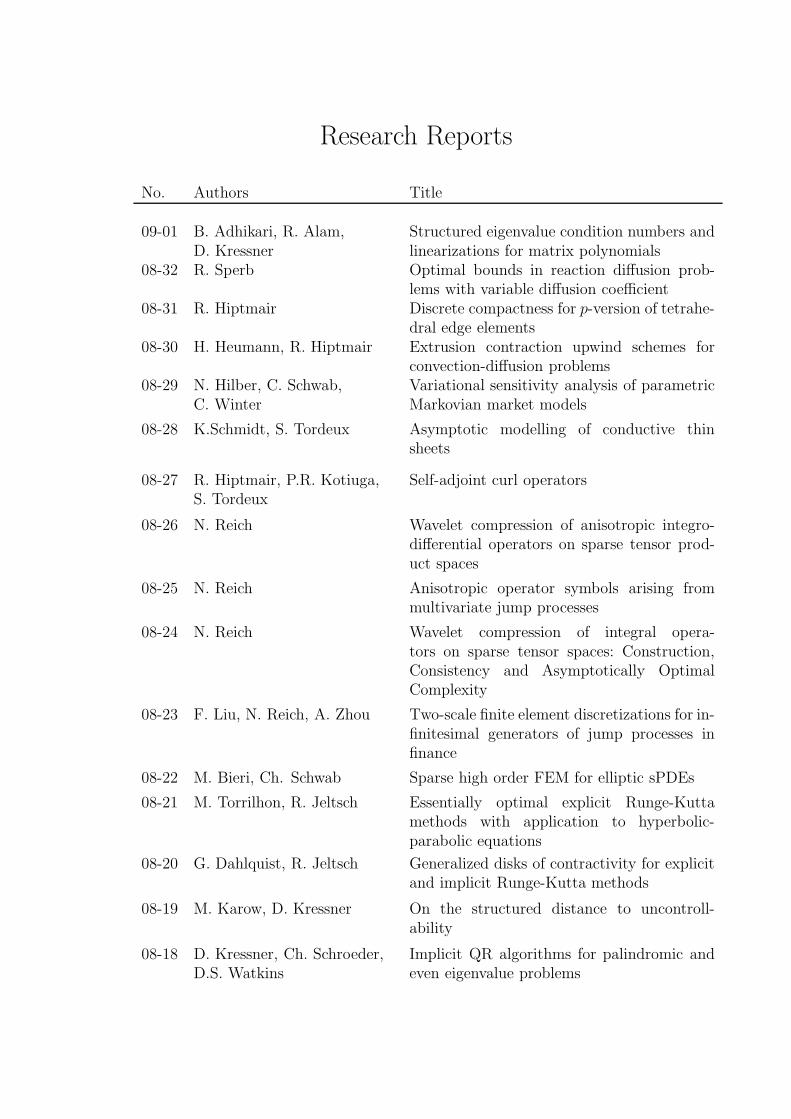
Research Reports
No. Authors Title
09-01 B. Adhikari, R. Alam,D. Kressner
Structured eigenvalue condition numbers andlinearizations for matrix polynomials
08-32 R. Sperb Optimal bounds in reaction di!usion prob-lems with variable di!usion coe"cient
08-31 R. Hiptmair Discrete compactness for p-version of tetrahe-dral edge elements
08-30 H. Heumann, R. Hiptmair Extrusion contraction upwind schemes forconvection-di!usion problems
08-29 N. Hilber, C. Schwab,C. Winter
Variational sensitivity analysis of parametricMarkovian market models
08-28 K.Schmidt, S. Tordeux Asymptotic modelling of conductive thinsheets
08-27 R. Hiptmair, P.R. Kotiuga,S. Tordeux
Self-adjoint curl operators
08-26 N. Reich Wavelet compression of anisotropic integro-di!erential operators on sparse tensor prod-uct spaces
08-25 N. Reich Anisotropic operator symbols arising frommultivariate jump processes
08-24 N. Reich Wavelet compression of integral opera-tors on sparse tensor spaces: Construction,Consistency and Asymptotically OptimalComplexity
08-23 F. Liu, N. Reich, A. Zhou Two-scale finite element discretizations for in-finitesimal generators of jump processes infinance
08-22 M. Bieri, Ch. Schwab Sparse high order FEM for elliptic sPDEs
08-21 M. Torrilhon, R. Jeltsch Essentially optimal explicit Runge-Kuttamethods with application to hyperbolic-parabolic equations
08-20 G. Dahlquist, R. Jeltsch Generalized disks of contractivity for explicitand implicit Runge-Kutta methods
08-19 M. Karow, D. Kressner On the structured distance to uncontroll-ability
08-18 D. Kressner, Ch. Schroeder,D.S. Watkins
Implicit QR algorithms for palindromic andeven eigenvalue problems