1

School of Computer Science

Probabilistic Graphical ModelsProbabilistic Graphical Models

Structured Sparse Additive ModelsStructured Sparse Additive Models

JunmingJunming Yin and Eric Yin and Eric XingXingLecture 27, April 24, 2013

Reading: See class website1© Eric Xing @ CMU, 2005-2013

OutlineNonparametric regression and kernel smoothing

Additive models

Sparse additive models (SpAM)

Structured sparse additive models (GroupSpAM)p ( p p )

2© Eric Xing @ CMU, 2005-2013

2

Nonparametric Regression Nonparametric Regression and Kernel Smoothingand Kernel Smoothing

3© Eric Xing @ CMU, 2005-2013

Non-linear functions:

4© Eric Xing @ CMU, 2005-2013

3

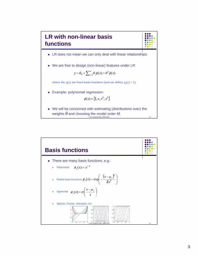
LR with non-linear basis functions

LR does not mean we can only deal with linear relationships

We are free to design (non-linear) features under LR

where the φj(x) are fixed basis functions (and we define φ0(x) = 1).

)()( xxy Tm

j j φθφθθ =+= ∑ =10

Example: polynomial regression:

We will be concerned with estimating (distributions over) the weights θ and choosing the model order M.

[ ]321 xxxx ,,,:)( =φ

5© Eric Xing @ CMU, 2005-2013

Basis functionsThere are many basis functions, e.g.:

P l i l 1−j)(φPolynomial

Radial basis functions

Sigmoidal

1= jj xx)(φ

( )⎟⎟⎠

⎞⎜⎜⎝

⎛ −−= 2

2

2sx

x jj

µφ exp)(

⎟⎟⎠

⎞⎜⎜⎝

⎛ −=

sx

x jj

µσφ )(

Splines, Fourier, Wavelets, etc

⎠⎝ s

6© Eric Xing @ CMU, 2005-2013

4

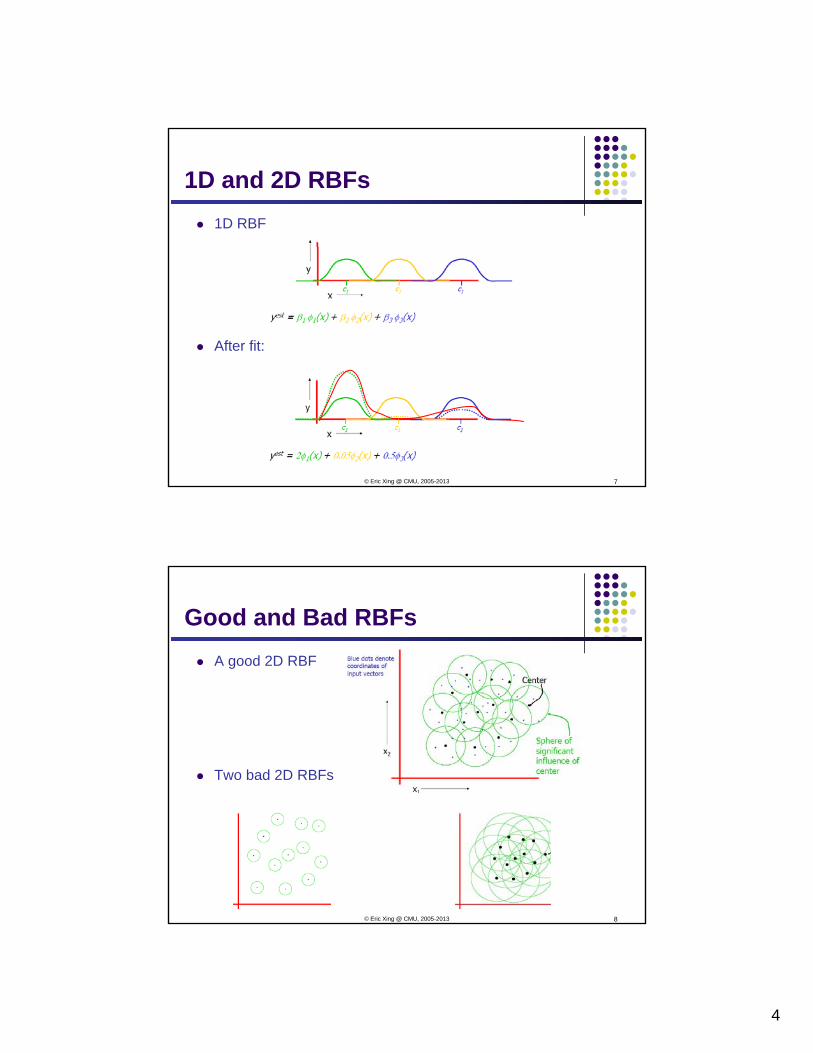
1D and 2D RBFs1D RBF

After fit:

7© Eric Xing @ CMU, 2005-2013

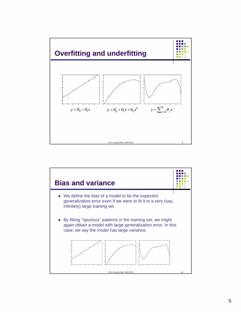
Good and Bad RBFsA good 2D RBF

Two bad 2D RBFs

8© Eric Xing @ CMU, 2005-2013

5

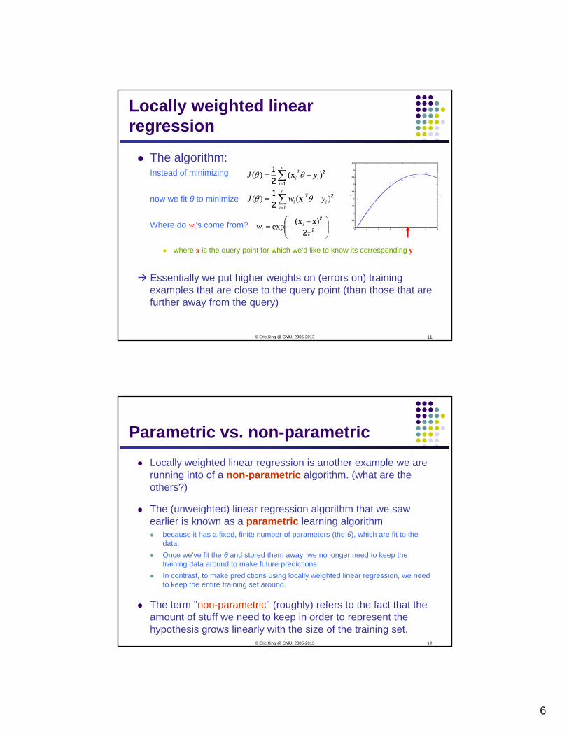
Overfitting and underfitting

θθ + 2θθθ ++ ∑5 jθxy 10 θθ += 2210 xxy θθθ ++= ∑ =

=0j

jj xy θ

9© Eric Xing @ CMU, 2005-2013

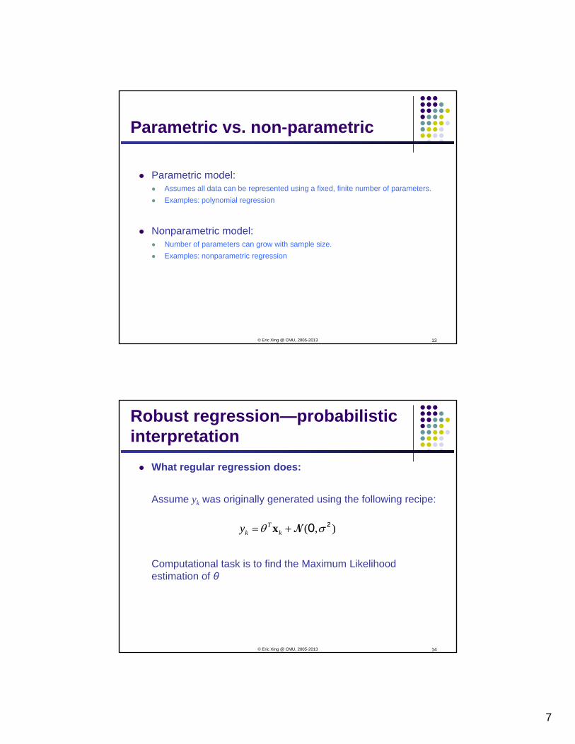
Bias and varianceWe define the bias of a model to be the expected generalization error even if we were to fit it to a very (say, g y ( y,infinitely) large training set.

By fitting "spurious" patterns in the training set, we might again obtain a model with large generalization error. In this case, we say the model has large variance.

10© Eric Xing @ CMU, 2005-2013

6

Locally weighted linear regression

The algorithm:Instead of minimizing ∑

nTJ 21 )()( θθInstead of minimizing

now we fit θ to minimize

Where do wi's come from?

where x is the query point for which we'd like to know its corresponding y

∑=

−=i

ii yJ1

2

2)()( θθ x

∑=

−=n

ii

Tii ywJ

1

2

21 )()( θθ x

⎟⎟⎠

⎞⎜⎜⎝

⎛ −−= 2

2

2τ)(exp xxi

iw

Essentially we put higher weights on (errors on) training examples that are close to the query point (than those that are further away from the query)

11© Eric Xing @ CMU, 2005-2013

Parametric vs. non-parametricLocally weighted linear regression is another example we are running into of a non-parametric algorithm. (what are the g p g (others?)

The (unweighted) linear regression algorithm that we saw earlier is known as a parametric learning algorithm

because it has a fixed, finite number of parameters (the θ), which are fit to the data;Once we've fit the θ and stored them away, we no longer need to keep the training data around to make future predictionstraining data around to make future predictions.In contrast, to make predictions using locally weighted linear regression, we need to keep the entire training set around.

The term "non-parametric" (roughly) refers to the fact that the amount of stuff we need to keep in order to represent the hypothesis grows linearly with the size of the training set.

12© Eric Xing @ CMU, 2005-2013

7

Parametric model:

Parametric vs. non-parametric

Parametric model:Assumes all data can be represented using a fixed, finite number of parameters.Examples: polynomial regression

Nonparametric model:Number of parameters can grow with sample size.Examples: nonparametric regressionp p g

13© Eric Xing @ CMU, 2005-2013

Robust regression—probabilistic interpretation

What regular regression does:

Assume yk was originally generated using the following recipe:

Computational task is to find the Maximum Likelihood

),( 20 σθ N+= kT

ky x

pestimation of θ

14© Eric Xing @ CMU, 2005-2013

8

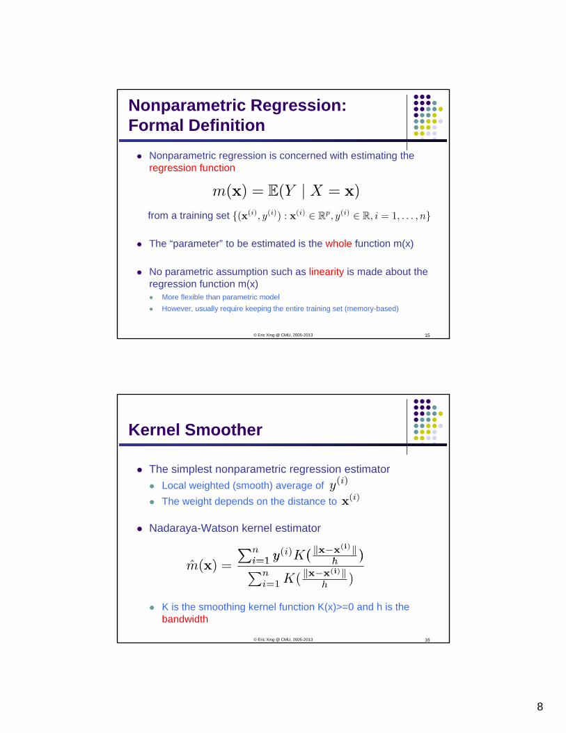
Nonparametric regression is concerned with estimating the regression function

Nonparametric Regression: Formal Definition

g

from a training set

The “parameter” to be estimated is the whole function m(x)

No parametric assumption such as linearity is made about the regression function m(x)

More flexible than parametric modelHowever, usually require keeping the entire training set (memory-based)

15© Eric Xing @ CMU, 2005-2013

Kernel Smoother

The simplest nonparametric regression estimatorLocal weighted (smooth) average ofThe weight depends on the distance to

Nadaraya-Watson kernel estimator

K is the smoothing kernel function K(x)>=0 and h is the bandwidth

16© Eric Xing @ CMU, 2005-2013

9

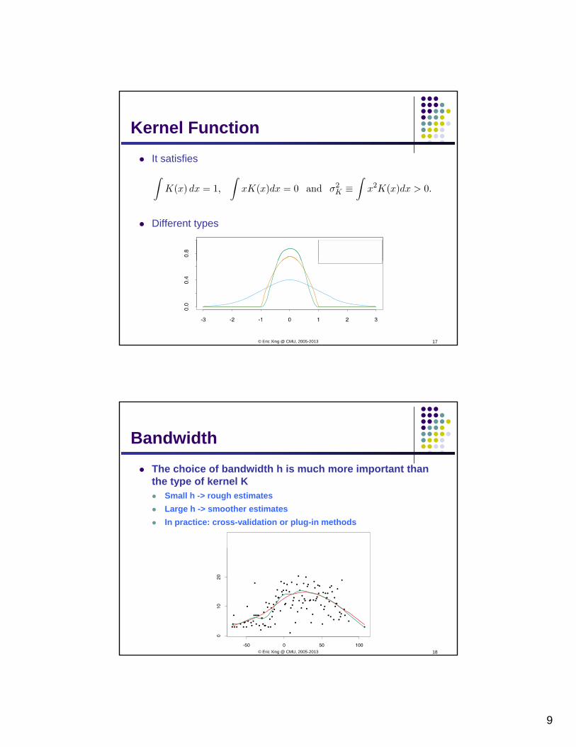
It satisfies

Kernel Function

Different types

17© Eric Xing @ CMU, 2005-2013

BandwidthThe choice of bandwidth h is much more important than the type of kernel Kyp

Small h -> rough estimatesLarge h -> smoother estimatesIn practice: cross-validation or plug-in methods

18© Eric Xing @ CMU, 2005-2013

10

Linear Smoothers

Kernel smoothers are examples of linear smoothers

For each x, the estimator is a linear combination of

Other examples: smoothing splines, locally weighted polynomial, etc

19© Eric Xing @ CMU, 2005-2013

Linear Smoothers (con’t)Define be the fitted values of the training examples, theng p ,

The n x n matrix S is called the smoother matrix with

The fitted values are the smoother version of original values

Recall the regression function can be gviewed as

P is the conditional expectation operator that projects a random variable (it is Y here) onto the linear space of XIt plays the role of smoother in the population setting

20© Eric Xing @ CMU, 2005-2013

11

Additive ModelsAdditive Models

21© Eric Xing @ CMU, 2005-2013

Additive ModelsDue to curse of dimensionality, smoothers break down in high dimensional settinggHastie & Tibshirani (1990) proposed the additive model

Each is a smooth one-dimensional component function

However, the model is not identifiableCan add a constant to one component function and subtract the same constant from another component

Can be easily fixed by assuming

22© Eric Xing @ CMU, 2005-2013

12

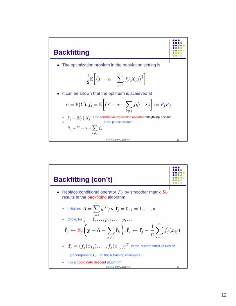
BackfittingThe optimization problem in the population setting is

It can be shown that the optimum is achieved at

is the conditional expectation operator onto jth input spaceis the partial residual

23© Eric Xing @ CMU, 2005-2013

Backfitting (con’t)Replace conditional operator by smoother matrixresults in the backfitting algorithmg g

Initialize:

Cycle: for

is the current fitted values of

jth component on the n training examples

It is a coordinate descent algorithm24© Eric Xing @ CMU, 2005-2013

13

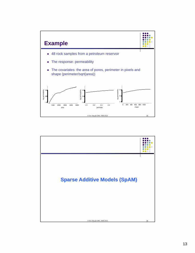
Example48 rock samples from a petroleum reservoir

The response: permeability

The covariates: the area of pores, perimeter in pixels and shape (perimeter/sqrt(area))

25© Eric Xing @ CMU, 2005-2013

Sparse Additive Models (SpAM)Sparse Additive Models (SpAM)

26© Eric Xing @ CMU, 2005-2013

14

SpAMA sparse version of additive models (Ravikumar et. al 2009)Can perform component/variable selection for additive modelsCan perform component/variable selection for additive models even when n << pThe optimization problem in the population setting is

behaves like an l1 ball across different components

to encourage functional sparsity

If each component function is constrained to have the linear form, the formulation reduces to standard lasso (Tibshirani 1996)

27© Eric Xing @ CMU, 2005-2013

SpAM BackfittingThe optimum is achieved by soft-thresholding step

is the partial residual; is the positive part(thresholding condition)

As in standard additive models, replace by p y

is the empirical estimate of

28© Eric Xing @ CMU, 2005-2013

15

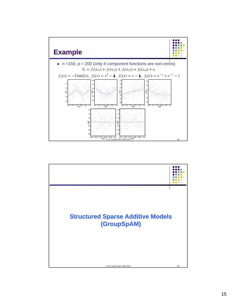
Examplen =150, p = 200 (only 4 component functions are non-zeros)

29© Eric Xing @ CMU, 2005-2013

Structured Sparse Structured Sparse Additive Models Additive Models ((GroupSpAMGroupSpAM))

30© Eric Xing @ CMU, 2005-2013

16

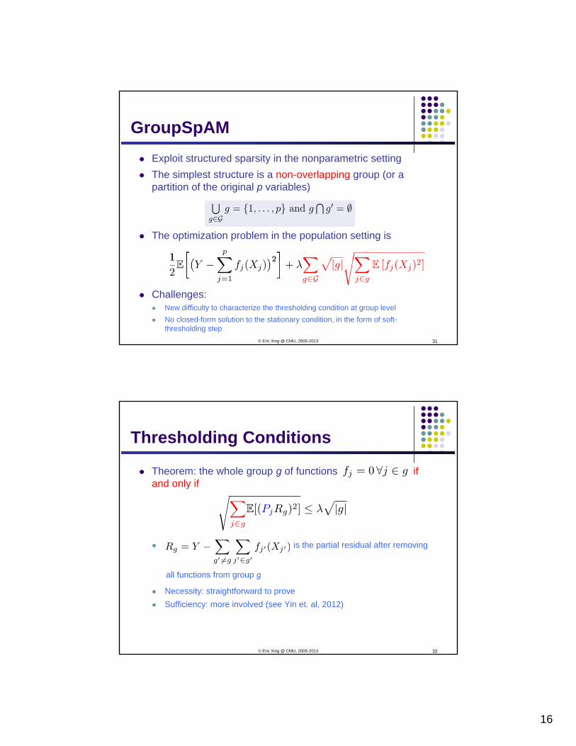
GroupSpAMExploit structured sparsity in the nonparametric settingThe simplest structure is a non-overlapping group (or aThe simplest structure is a non-overlapping group (or a partition of the original p variables)

The optimization problem in the population setting is

Challenges:New difficulty to characterize the thresholding condition at group levelNo closed-form solution to the stationary condition, in the form of soft-thresholding step

31© Eric Xing @ CMU, 2005-2013

Thresholding Conditions

Theorem: the whole group g of functions if and only ifand only if

is the partial residual after removing

all functions from group g

Necessity: straightforward to proveSufficiency: more involved (see Yin et. al, 2012)

32© Eric Xing @ CMU, 2005-2013

17

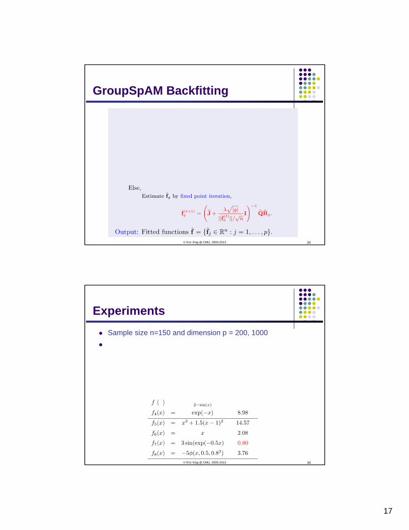
GroupSpAM Backfitting

33© Eric Xing @ CMU, 2005-2013

ExperimentsSample size n=150 and dimension p = 200, 1000

34© Eric Xing @ CMU, 2005-2013

18

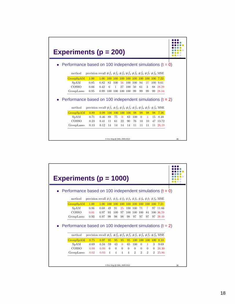
Experiments (p = 200)Performance based on 100 independent simulations (t = 0)

Performance based on 100 independent simulations (t = 2)

35© Eric Xing @ CMU, 2005-2013

Experiments (p = 1000)Performance based on 100 independent simulations (t = 0)

Performance based on 100 independent simulations (t = 2)

36© Eric Xing @ CMU, 2005-2013

19

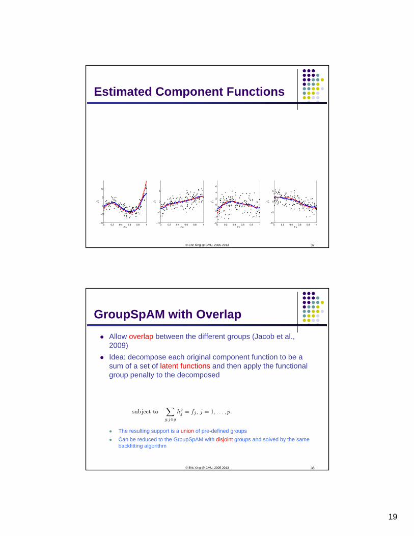
Estimated Component Functions

37© Eric Xing @ CMU, 2005-2013

GroupSpAM with OverlapAllow overlap between the different groups (Jacob et al., 2009))Idea: decompose each original component function to be a sum of a set of latent functions and then apply the functional group penalty to the decomposed

The resulting support is a union of pre-defined groupsCan be reduced to the GroupSpAM with disjoint groups and solved by the same backfitting algorithm

38© Eric Xing @ CMU, 2005-2013

20

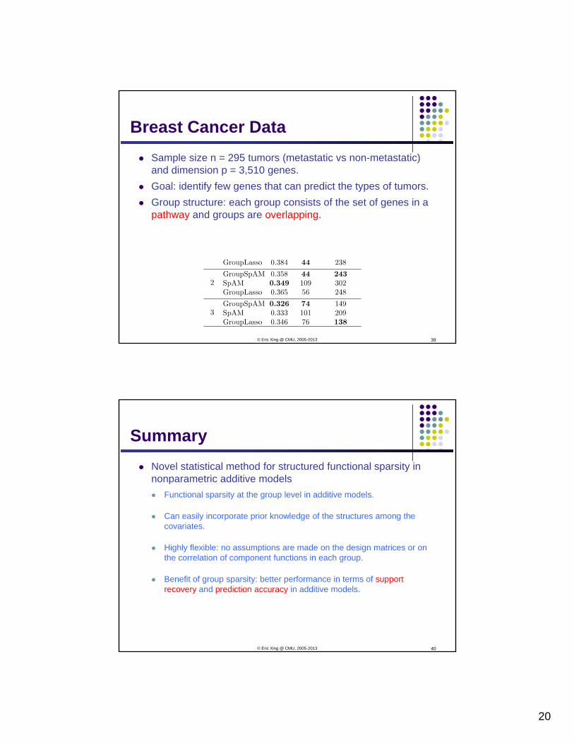
Breast Cancer DataSample size n = 295 tumors (metastatic vs non-metastatic) and dimension p = 3,510 genes.p , gGoal: identify few genes that can predict the types of tumors.Group structure: each group consists of the set of genes in a pathway and groups are overlapping.

39© Eric Xing @ CMU, 2005-2013

SummaryNovel statistical method for structured functional sparsity in nonparametric additive modelsp

Functional sparsity at the group level in additive models.

Can easily incorporate prior knowledge of the structures among the covariates.

Highly flexible: no assumptions are made on the design matrices or on the correlation of component functions in each group.

Benefit of group sparsity: better performance in terms of support recovery and prediction accuracy in additive models.

40© Eric Xing @ CMU, 2005-2013

21

References

Hastie T and Tibshirani R Generalized Additive ModelsHastie, T. and Tibshirani, R. Generalized Additive Models. Chapman & Hall/CRC, 1990.Buja, A., Hastie, T., and Tibshirani, R. Linear Smoothers and Additive Models. Ann. Statist. Volume 17, Number 2 (1989), 453-510.Ravikumar, P., Lafferty, J., Liu, H., and Wasserman, L. Sparse additive models. JRSSB, 71(5):1009–1030, 2009.Sparse additive models. JRSSB, 71(5):1009 1030, 2009.Yin, J., Chen, X., and Xing, E. Group Sparse Additive Models, ICML, 2012

41© Eric Xing @ CMU, 2005-2013