Embed Size (px)
Citation preview

Structured sparsity-inducing normsthrough submodular functions
Francis Bach
Willow project, INRIA - Ecole Normale Superieure
NIPS - December 7, 2010
Outline
• Introduction: Sparse methods for machine learning
– Need for structured sparsity: Going beyond the ℓ1-norm
• Submodular functions
– Lovasz extension
• Structured sparsity through submodular functions
– Relaxation of the penalization of supports
– Examples
– Unified algorithms and analysis
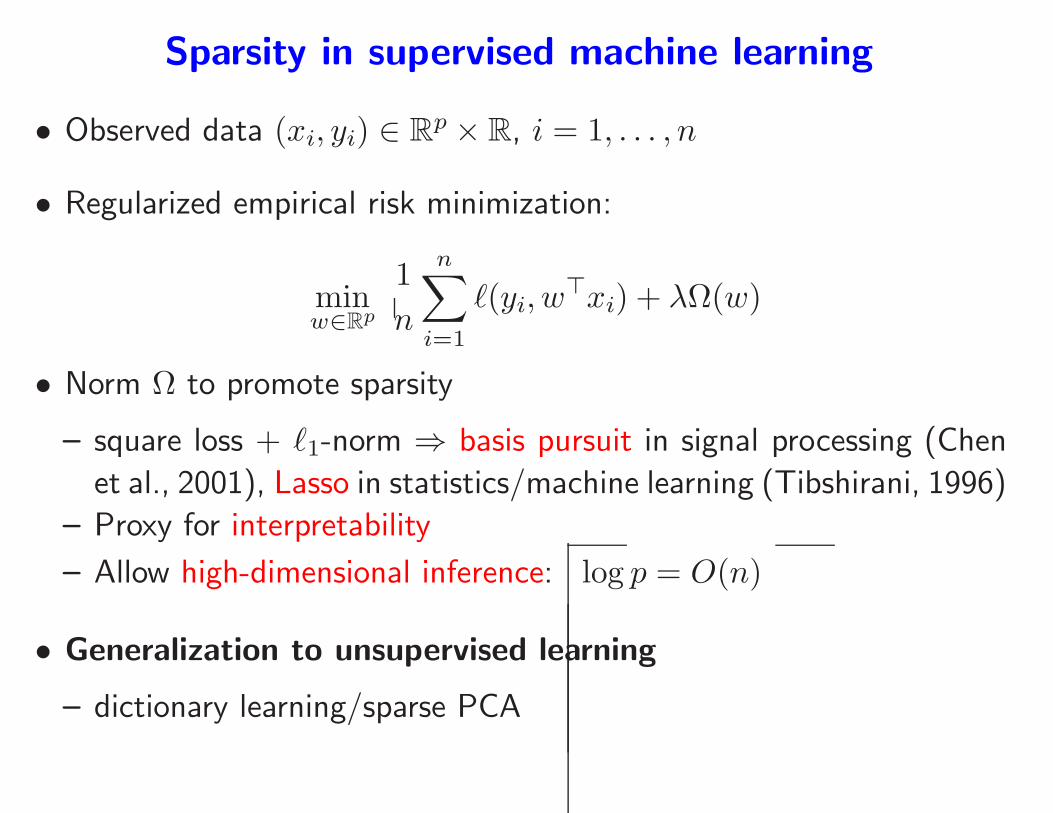
Sparsity in supervised machine learning
• Observed data (xi, yi) ∈ Rp × R, i = 1, . . . , n
• Regularized empirical risk minimization:
minw∈Rp
1
n
n∑
i=1
ℓ(yi, w⊤xi) + λΩ(w)
• Norm Ω to promote sparsity
– square loss + ℓ1-norm ⇒ basis pursuit in signal processing (Chen
et al., 2001), Lasso in statistics/machine learning (Tibshirani, 1996)
– Proxy for interpretability
– Allow high-dimensional inference: log p = O(n)
• Generalization to unsupervised learning
– dictionary learning/sparse PCA
Why structured sparsity?
• Interpretability
– Structured dictionary elements (Jenatton et al., 2009b)
– Dictionary elements “organized” in a tree or a grid (Kavukcuoglu
et al., 2009; Jenatton et al., 2010; Mairal et al., 2010)
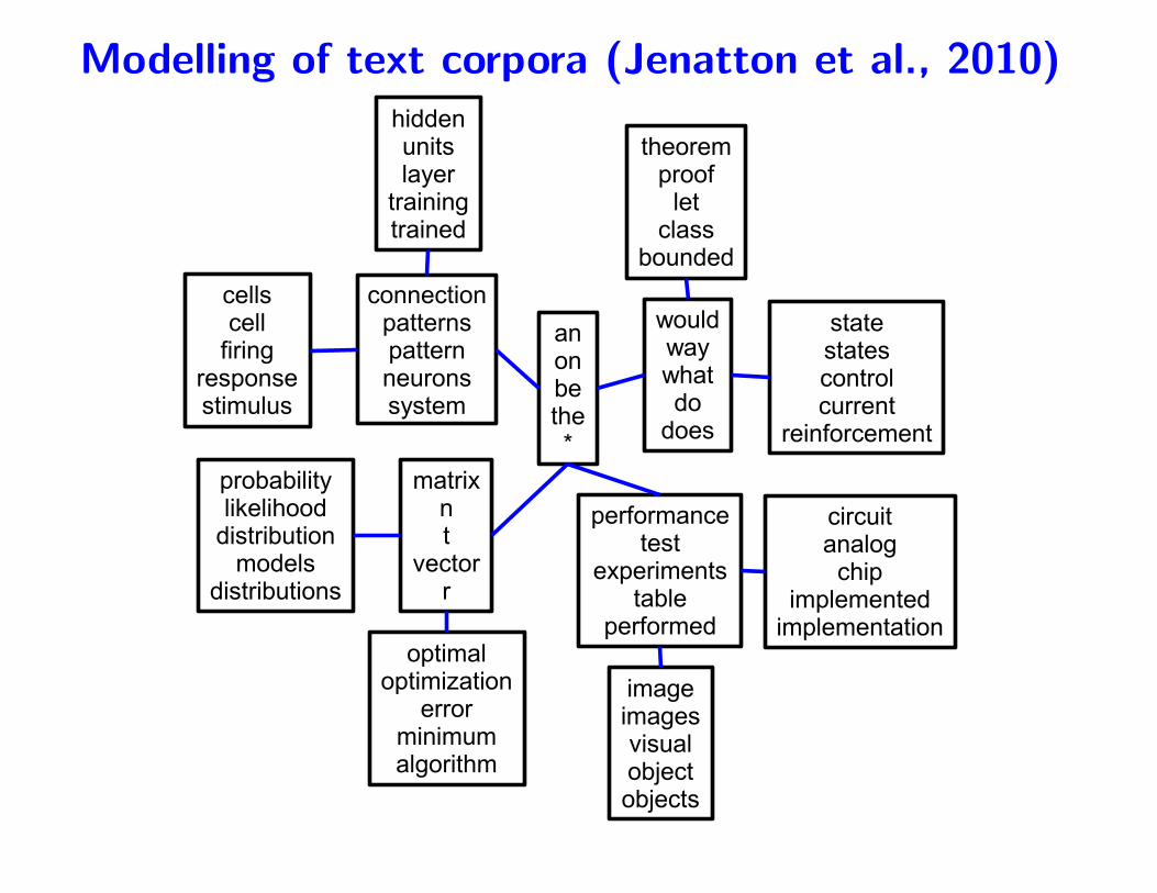
Modelling of text corpora (Jenatton et al., 2010)
Why structured sparsity?
• Interpretability
– Structured dictionary elements (Jenatton et al., 2009b)
– Dictionary elements “organized” in a tree or a grid (Kavukcuoglu
et al., 2009; Jenatton et al., 2010; Mairal et al., 2010)
• Predictive performance
– When prior knowledge matches data
• Numerical efficiency
– Non-linear variable selection with 2p subsets (Bach, 2008)
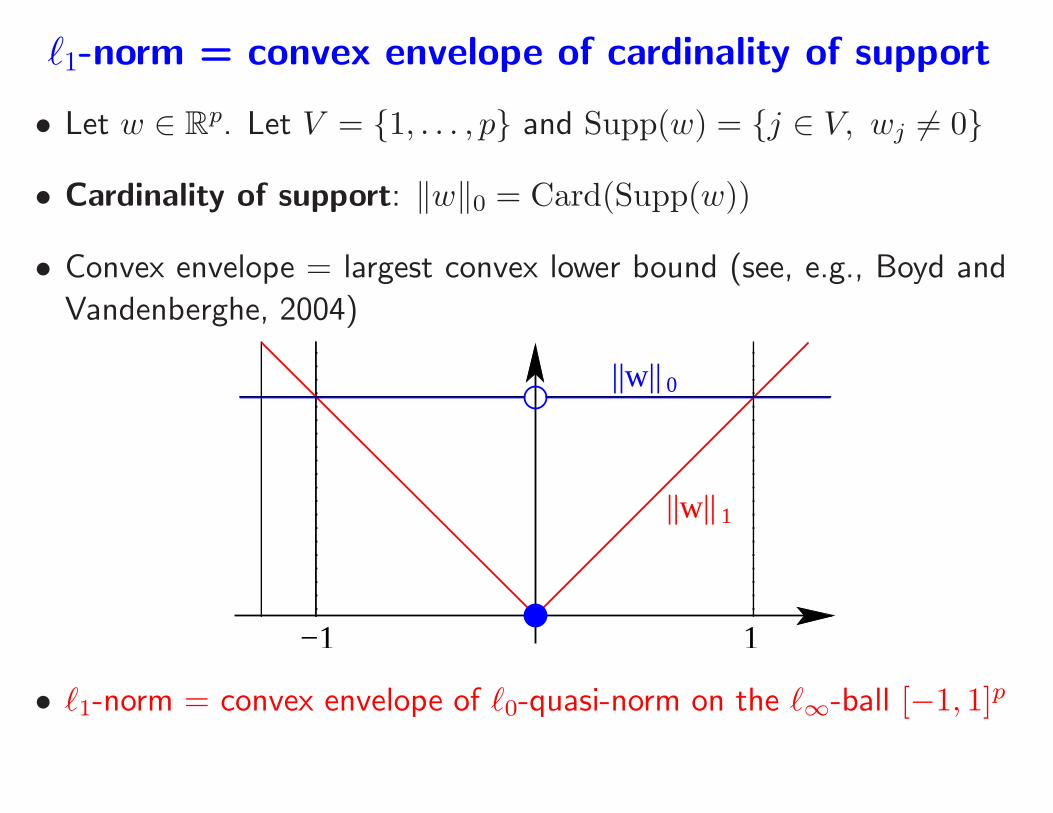
ℓ1-norm = convex envelope of cardinality of support
• Let w ∈ Rp. Let V = 1, . . . , p and Supp(w) = j ∈ V, wj 6= 0
• Cardinality of support: ‖w‖0 = Card(Supp(w))
• Convex envelope = largest convex lower bound (see, e.g., Boyd and
Vandenberghe, 2004)
1
0
||w||
||w||
−1 1
• ℓ1-norm = convex envelope of ℓ0-quasi-norm on the ℓ∞-ball [−1, 1]p
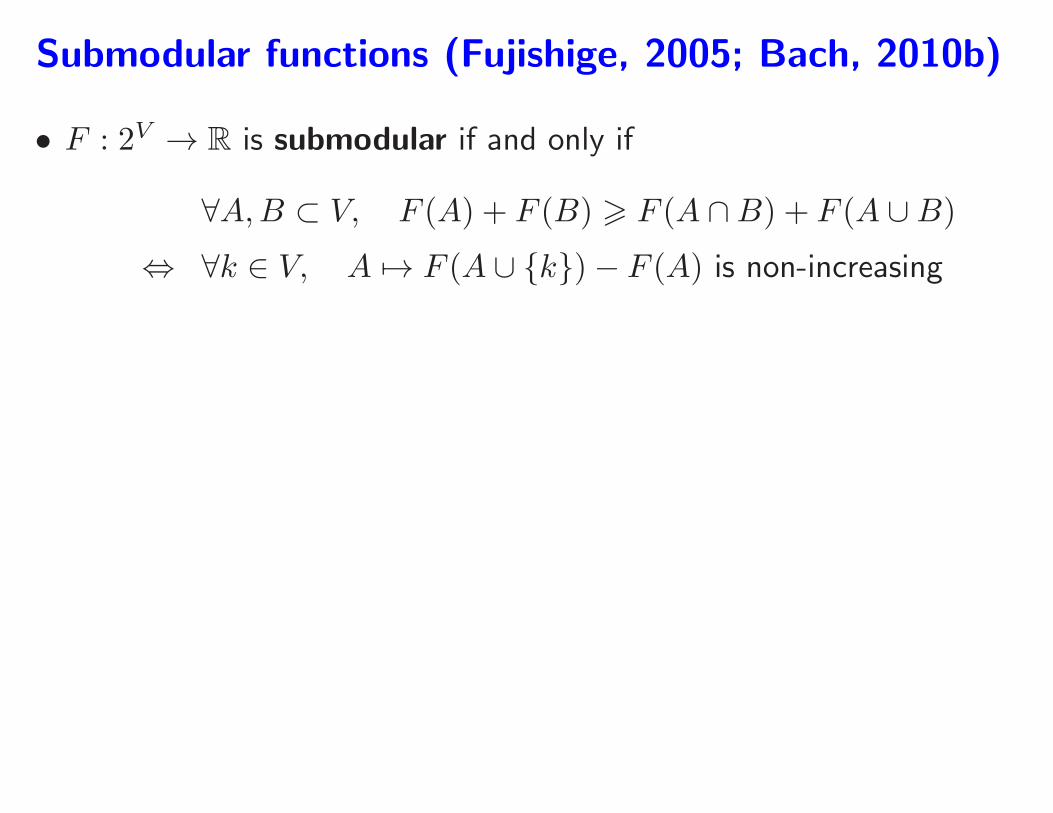
Submodular functions (Fujishige, 2005; Bach, 2010b)
• F : 2V → R is submodular if and only if
∀A,B ⊂ V, F (A) + F (B) > F (A ∩B) + F (A ∪B)
⇔ ∀k ∈ V, A 7→ F (A ∪ k)− F (A) is non-increasing
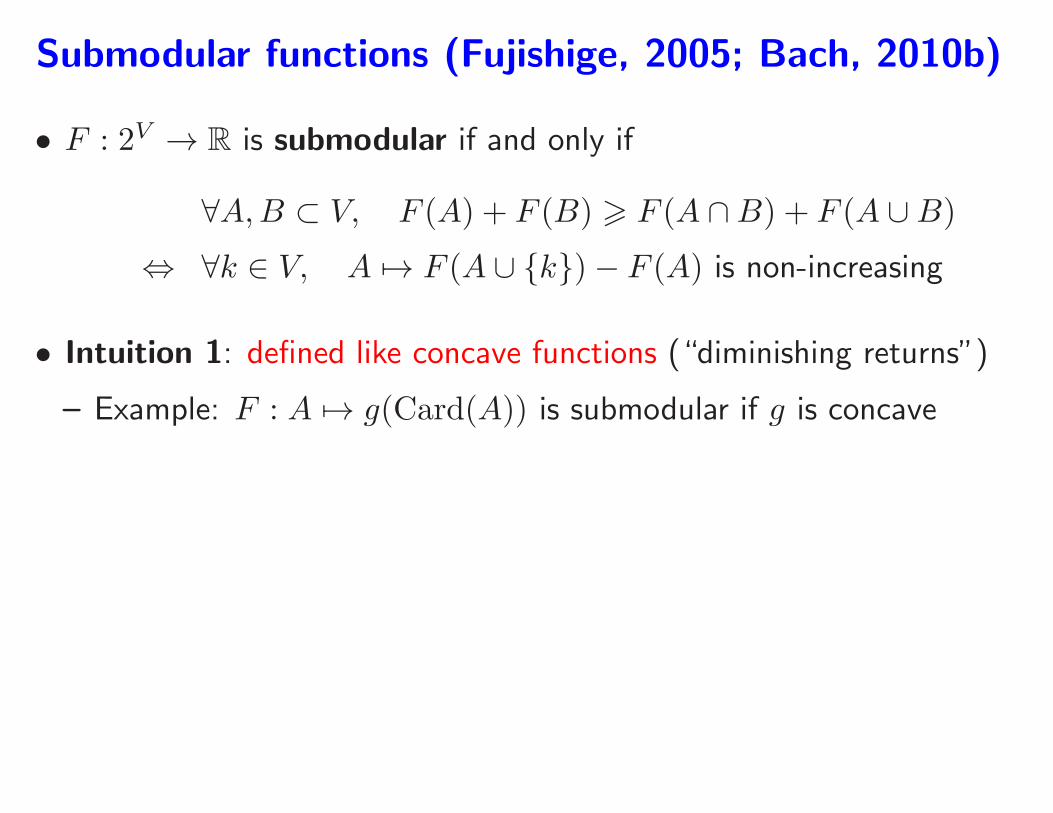
Submodular functions (Fujishige, 2005; Bach, 2010b)
• F : 2V → R is submodular if and only if
∀A,B ⊂ V, F (A) + F (B) > F (A ∩B) + F (A ∪B)
⇔ ∀k ∈ V, A 7→ F (A ∪ k)− F (A) is non-increasing
• Intuition 1: defined like concave functions (“diminishing returns”)
– Example: F : A 7→ g(Card(A)) is submodular if g is concave
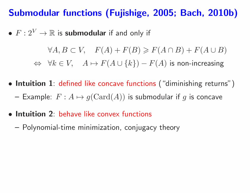
• Intuition 2: behave like convex functions
– Polynomial-time minimization, conjugacy theory
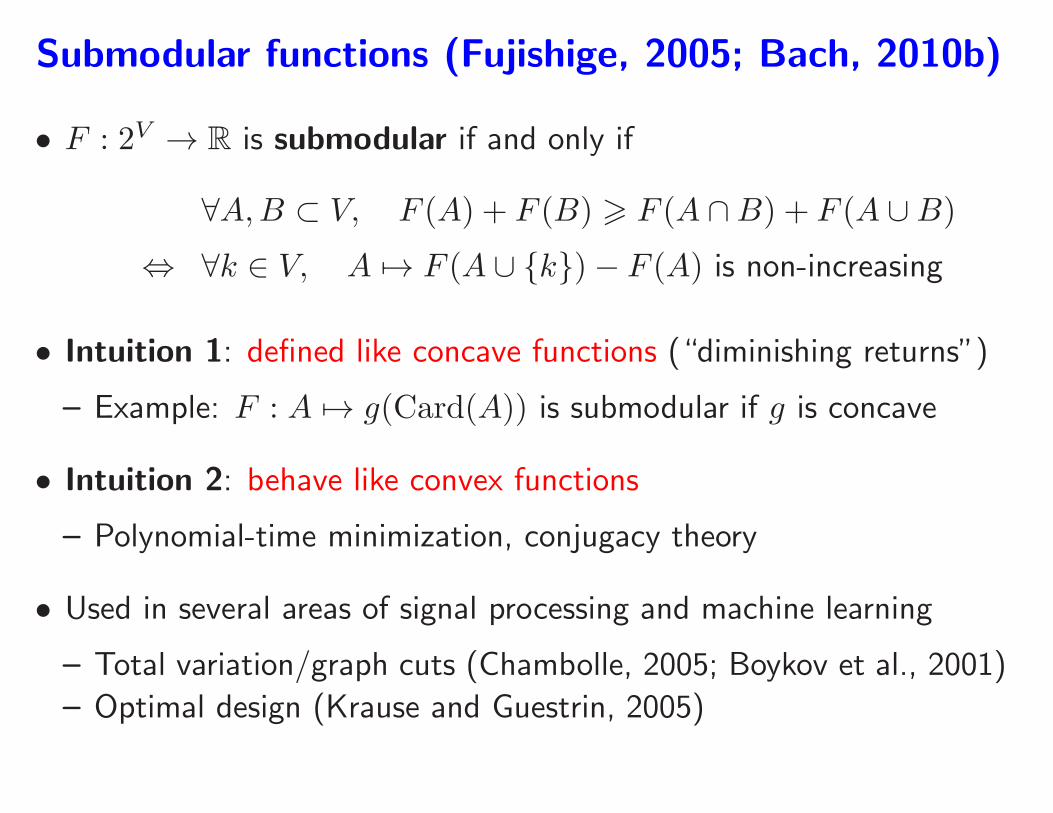
• Used in several areas of signal processing and machine learning
– Total variation/graph cuts (Chambolle, 2005; Boykov et al., 2001)
– Optimal design (Krause and Guestrin, 2005)
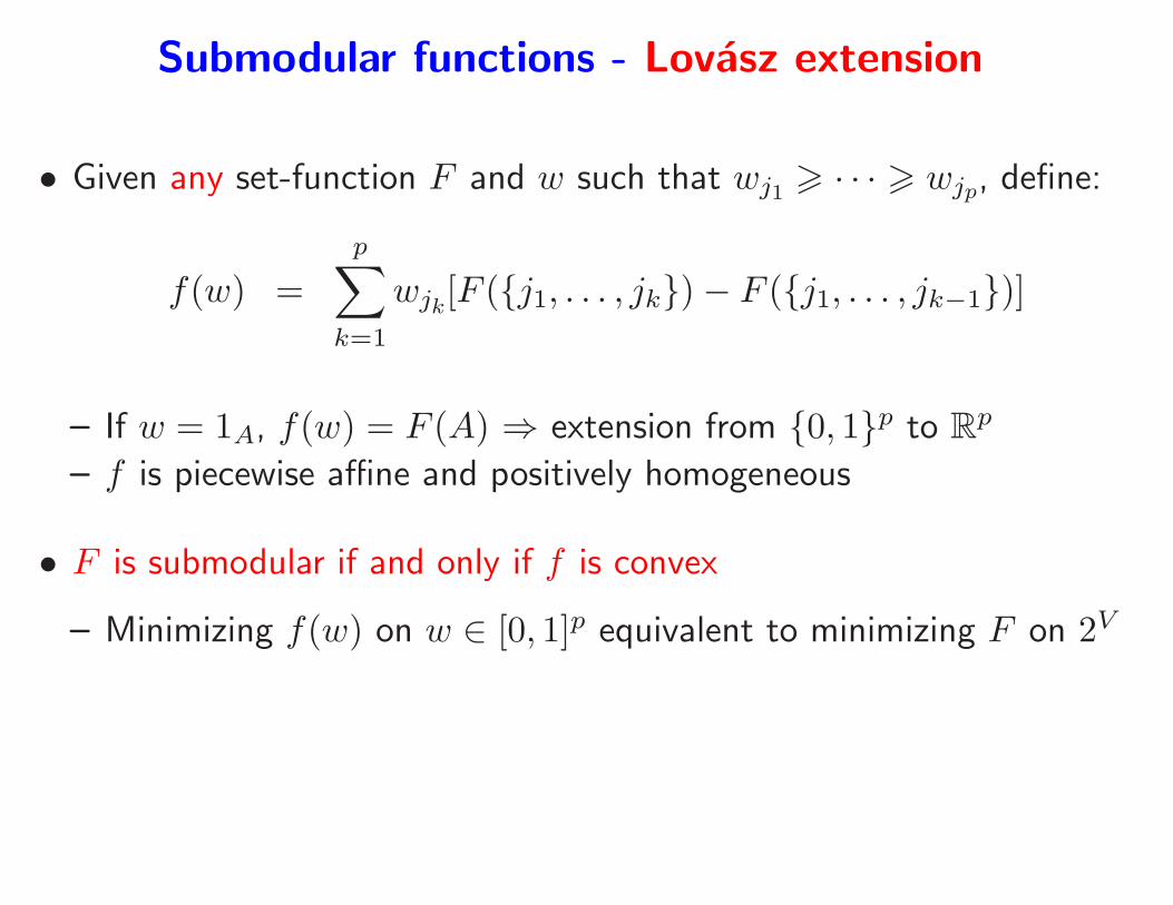
Submodular functions - Lovasz extension
• Given any set-function F and w such that wj1 > · · · > wjp, define:
f(w) =
p∑
k=1
wjk[F (j1, . . . , jk)− F (j1, . . . , jk−1)]
– If w = 1A, f(w) = F (A) ⇒ extension from 0, 1p to Rp
– f is piecewise affine and positively homogeneous
• F is submodular if and only if f is convex
– Minimizing f(w) on w ∈ [0, 1]p equivalent to minimizing F on 2V
Submodular functions and structured sparsity
• Let F : 2V → R be a non-decreasing submodular set-function
• Proposition: the convex envelope of Θ : w 7→ F (Supp(w)) on the
ℓ∞-ball is Ω : w 7→ f(|w|) where f is the Lovasz extension of F
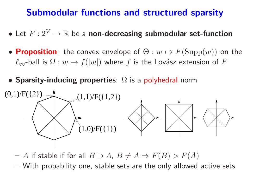
Submodular functions and structured sparsity
• Let F : 2V → R be a non-decreasing submodular set-function
• Proposition: the convex envelope of Θ : w 7→ F (Supp(w)) on the
ℓ∞-ball is Ω : w 7→ f(|w|) where f is the Lovasz extension of F
• Sparsity-inducing properties: Ω is a polyhedral norm
(1,0)/F(1)
(1,1)/F(1,2)(0,1)/F(2)
– A if stable if for all B ⊃ A, B 6= A ⇒ F (B) > F (A)
– With probability one, stable sets are the only allowed active sets
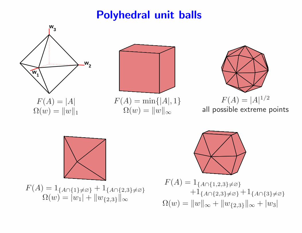
Polyhedral unit balls
w2
w3
w1
F (A) = |A|Ω(w) = ‖w‖1
F (A) = min|A|, 1Ω(w) = ‖w‖∞
F (A) = |A|1/2
all possible extreme points
F (A) = 1A∩16=∅ + 1A∩2,36=∅Ω(w) = |w1|+ ‖w2,3‖∞
F (A) = 1A∩1,2,36=∅+1A∩2,36=∅+1A∩36=∅
Ω(w) = ‖w‖∞ + ‖w2,3‖∞ + |w3|
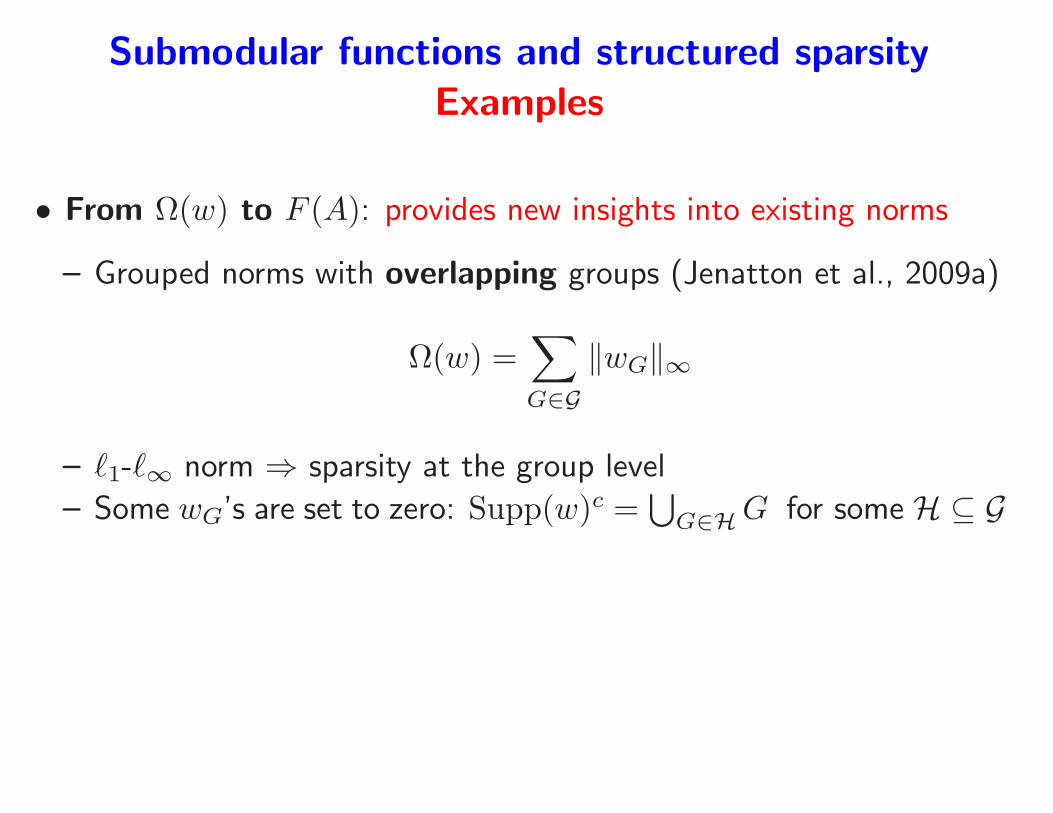
Submodular functions and structured sparsity
Examples
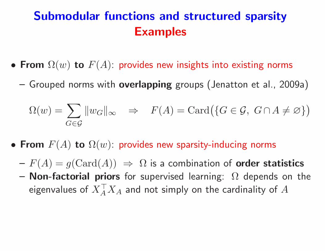
• From Ω(w) to F (A): provides new insights into existing norms
– Grouped norms with overlapping groups (Jenatton et al., 2009a)
Ω(w) =∑
G∈G‖wG‖∞
– ℓ1-ℓ∞ norm ⇒ sparsity at the group level
– Some wG’s are set to zero: Supp(w)c =⋃
G∈HG for some H ⊆ G
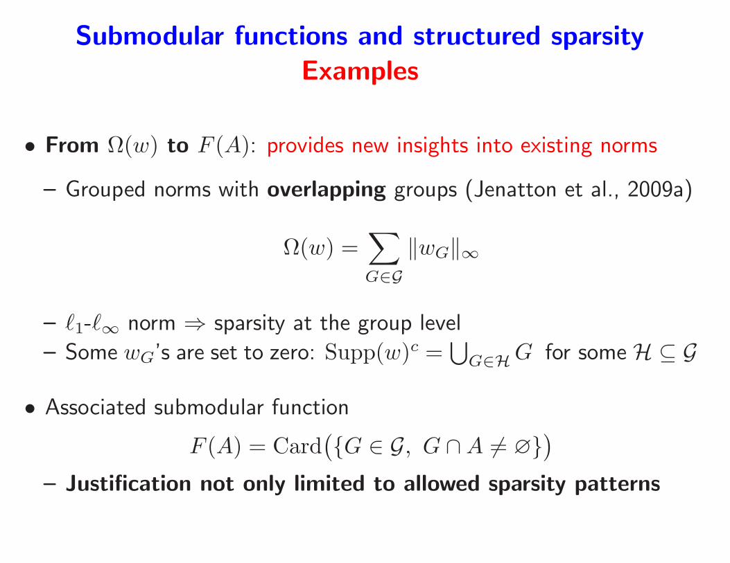
Submodular functions and structured sparsity
Examples
• From Ω(w) to F (A): provides new insights into existing norms
– Grouped norms with overlapping groups (Jenatton et al., 2009a)
Ω(w) =∑
G∈G‖wG‖∞
– ℓ1-ℓ∞ norm ⇒ sparsity at the group level
– Some wG’s are set to zero: Supp(w)c =⋃
G∈HG for some H ⊆ G
• Associated submodular function
F (A) = Card(
G ∈ G, G ∩A 6= ∅)
– Justification not only limited to allowed sparsity patterns
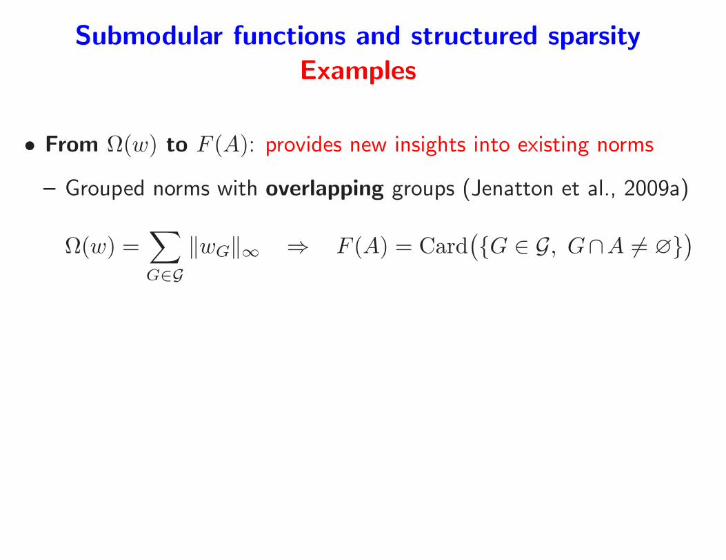
Submodular functions and structured sparsity
Examples
• From Ω(w) to F (A): provides new insights into existing norms
– Grouped norms with overlapping groups (Jenatton et al., 2009a)
Ω(w) =∑
G∈G‖wG‖∞ ⇒ F (A) = Card
(
G ∈ G, G∩A 6= ∅)
Submodular functions and structured sparsity
Examples
• From Ω(w) to F (A): provides new insights into existing norms
– Grouped norms with overlapping groups (Jenatton et al., 2009a)
Ω(w) =∑
G∈G‖wG‖∞ ⇒ F (A) = Card
(
G ∈ G, G∩A 6= ∅)
• From F (A) to Ω(w): provides new sparsity-inducing norms
– F (A) = g(Card(A)) ⇒ Ω is a combination of order statistics
– Non-factorial priors for supervised learning: Ω depends on the
eigenvalues of X⊤AXA and not simply on the cardinality of A
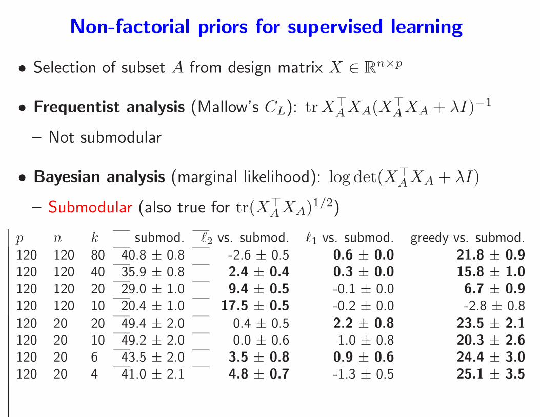
Non-factorial priors for supervised learning
• Selection of subset A from design matrix X ∈ Rn×p
• Frequentist analysis (Mallow’s CL): trX⊤AXA(X
⊤AXA + λI)−1
– Not submodular
• Bayesian analysis (marginal likelihood): log det(X⊤AXA + λI)
– Submodular (also true for tr(X⊤AXA)
1/2)
p n k submod. ℓ2 vs. submod. ℓ1 vs. submod. greedy vs. submod.120 120 80 40.8 ± 0.8 -2.6 ± 0.5 0.6 ± 0.0 21.8 ± 0.9120 120 40 35.9 ± 0.8 2.4 ± 0.4 0.3 ± 0.0 15.8 ± 1.0120 120 20 29.0 ± 1.0 9.4 ± 0.5 -0.1 ± 0.0 6.7 ± 0.9120 120 10 20.4 ± 1.0 17.5 ± 0.5 -0.2 ± 0.0 -2.8 ± 0.8120 20 20 49.4 ± 2.0 0.4 ± 0.5 2.2 ± 0.8 23.5 ± 2.1120 20 10 49.2 ± 2.0 0.0 ± 0.6 1.0 ± 0.8 20.3 ± 2.6120 20 6 43.5 ± 2.0 3.5 ± 0.8 0.9 ± 0.6 24.4 ± 3.0120 20 4 41.0 ± 2.1 4.8 ± 0.7 -1.3 ± 0.5 25.1 ± 3.5
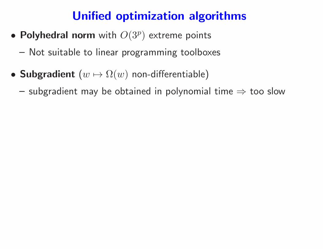
Unified optimization algorithms
• Polyhedral norm with O(3p) extreme points
– Not suitable to linear programming toolboxes
• Subgradient (w 7→ Ω(w) non-differentiable)
– subgradient may be obtained in polynomial time ⇒ too slow
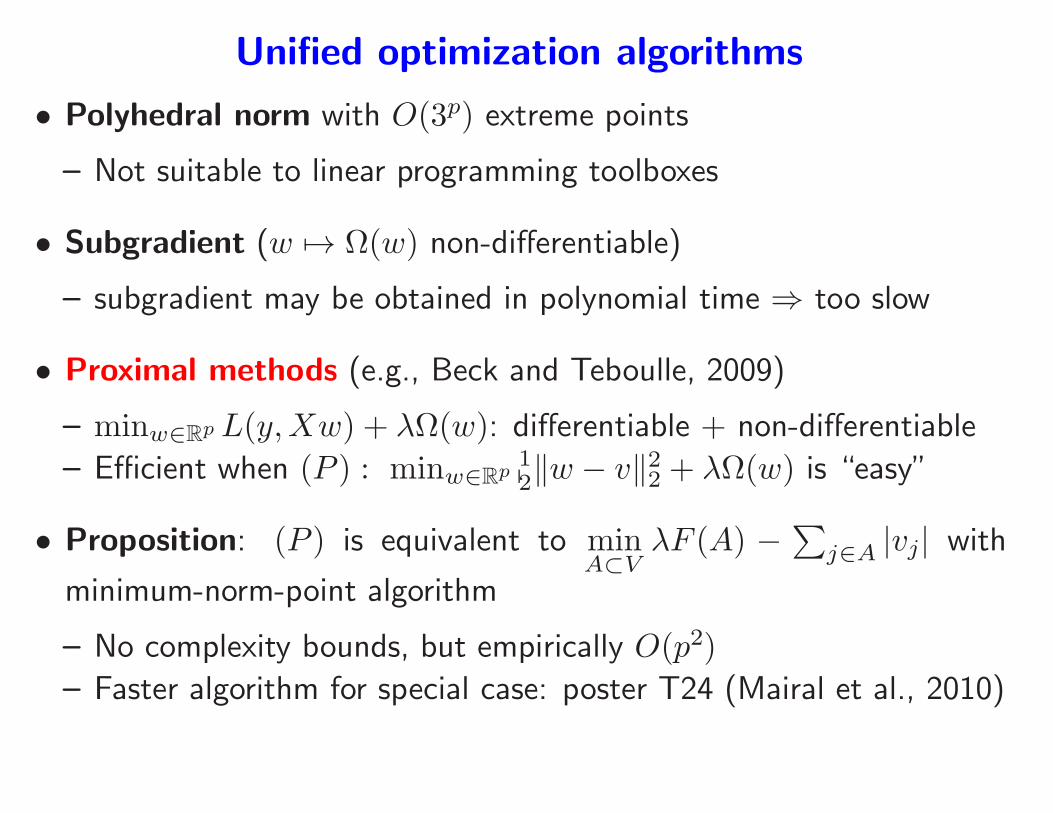
Unified optimization algorithms
• Polyhedral norm with O(3p) extreme points
– Not suitable to linear programming toolboxes
• Subgradient (w 7→ Ω(w) non-differentiable)
– subgradient may be obtained in polynomial time ⇒ too slow
• Proximal methods (e.g., Beck and Teboulle, 2009)
– minw∈Rp L(y,Xw) + λΩ(w): differentiable + non-differentiable
– Efficient when (P ) : minw∈Rp12‖w − v‖22 + λΩ(w) is “easy”
• Proposition: (P ) is equivalent to minA⊂V
λF (A) −∑
j∈A |vj| with
minimum-norm-point algorithm
– No complexity bounds, but empirically O(p2)
– Faster algorithm for special case: poster T24 (Mairal et al., 2010)
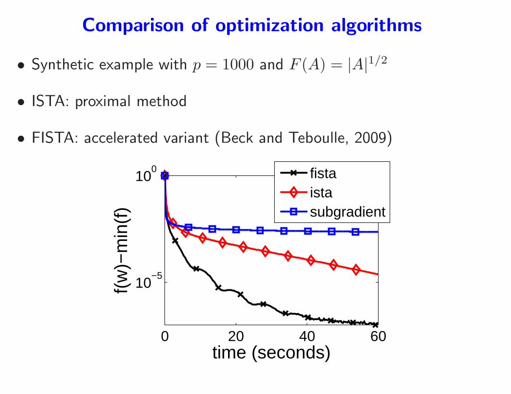
Comparison of optimization algorithms
• Synthetic example with p = 1000 and F (A) = |A|1/2
• ISTA: proximal method
• FISTA: accelerated variant (Beck and Teboulle, 2009)
0 20 40 60
10−5
100
time (seconds)
f(w
)−m
in(f
)
fistaistasubgradient
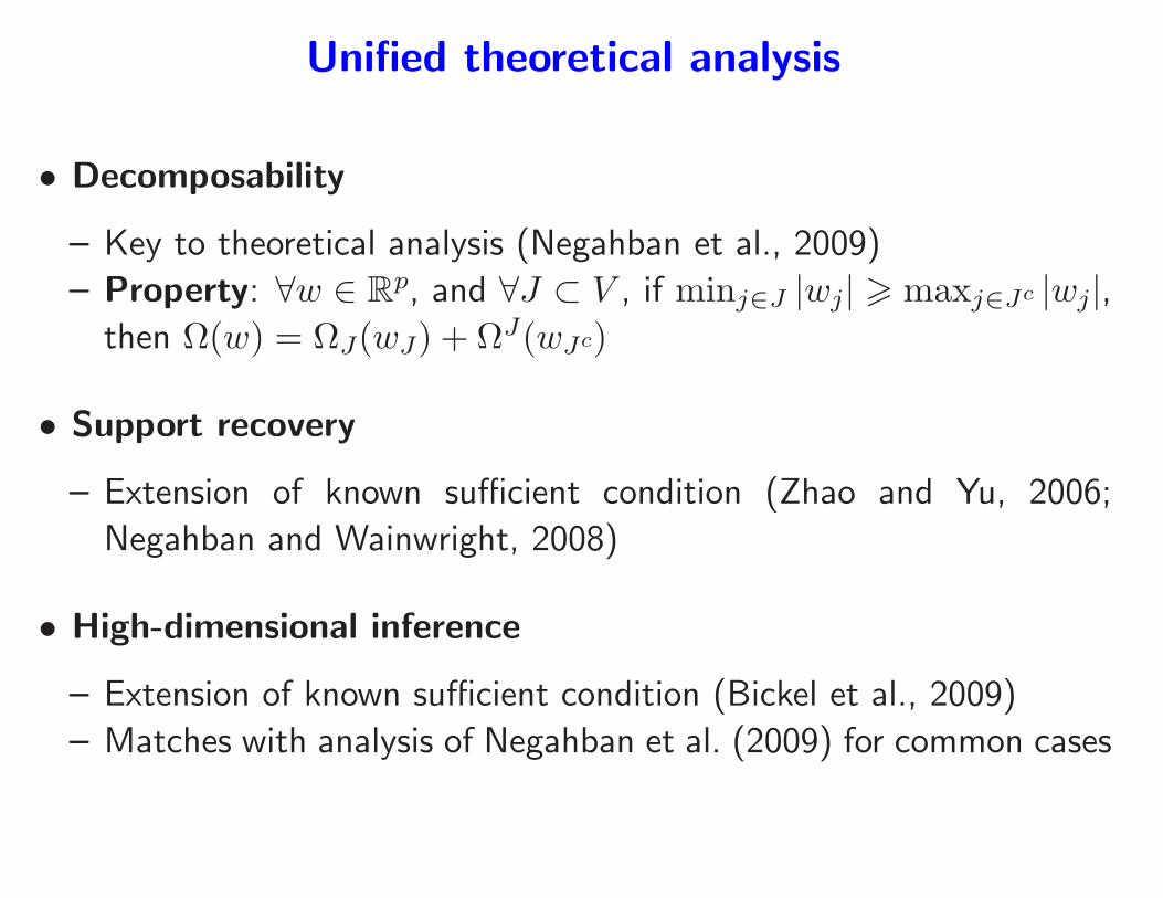
Unified theoretical analysis
• Decomposability
– Key to theoretical analysis (Negahban et al., 2009)
– Property: ∀w ∈ Rp, and ∀J ⊂ V , if minj∈J |wj| > maxj∈Jc |wj|,
then Ω(w) = ΩJ(wJ) + ΩJ(wJc)
• Support recovery
– Extension of known sufficient condition (Zhao and Yu, 2006;
Negahban and Wainwright, 2008)
• High-dimensional inference
– Extension of known sufficient condition (Bickel et al., 2009)
– Matches with analysis of Negahban et al. (2009) for common cases
Conclusion
• Structured sparsity through submodular functions
– Many applications (image, audio, text, etc.)
– Unified analysis and algorithms
Conclusion
• Structured sparsity through submodular functions
– Many applications (image, audio, text, etc.)
– Unified analysis and algorithms
• On-going work on structured sparsity
– Extension to symmetric submodular functions (Bach, 2010a)
∗ Shaping all level sets w = α, α ∈ R, rather than only α = 0
– Norm design beyond submodular functions
– Links with greedy methods (Haupt and Nowak, 2006; Huang et al.,
2009)
– Extensions to matrices

References
F. Bach. Exploring large feature spaces with hierarchical multiple kernel learning. In Advances in
Neural Information Processing Systems, 2008.
F. Bach. Shaping level sets with submodular functions. Technical Report 00542949, HAL, 2010a.
F. Bach. Convex analysis and optimization with submodular functions: a tutorial. Technical Report
00527714, HAL, 2010b.
A. Beck and M. Teboulle. A fast iterative shrinkage-thresholding algorithm for linear inverse problems.
SIAM Journal on Imaging Sciences, 2(1):183–202, 2009.
P. Bickel, Y. Ritov, and A. Tsybakov. Simultaneous analysis of Lasso and Dantzig selector. Annals of
Statistics, 37(4):1705–1732, 2009.
S. P. Boyd and L. Vandenberghe. Convex Optimization. Cambridge University Press, 2004.
Y. Boykov, O. Veksler, and R. Zabih. Fast approximate energy minimization via graph cuts. IEEE
Trans. PAMI, 23(11):1222–1239, 2001.
A. Chambolle. Total variation minimization and a class of binary MRF models. In Energy Minimization
Methods in Computer Vision and Pattern Recognition, pages 136–152. Springer, 2005.
S. S. Chen, D. L. Donoho, and M. A. Saunders. Atomic decomposition by basis pursuit. SIAM Review,
43(1):129–159, 2001.
S. Fujishige. Submodular Functions and Optimization. Elsevier, 2005.
J. Haupt and R. Nowak. Signal reconstruction from noisy random projections. IEEE Transactions on
Information Theory, 52(9):4036–4048, 2006.
J. Huang, T. Zhang, and D. Metaxas. Learning with structured sparsity. In Proceedings of the 26th
International Conference on Machine Learning (ICML), 2009.
R. Jenatton, J.Y. Audibert, and F. Bach. Structured variable selection with sparsity-inducing norms.
Technical report, arXiv:0904.3523, 2009a.
R. Jenatton, G. Obozinski, and F. Bach. Structured sparse principal component analysis. Technical
report, arXiv:0909.1440, 2009b.
R. Jenatton, J. Mairal, G. Obozinski, and F. Bach. Proximal methods for sparse hierarchical dictionary
learning. In Submitted to ICML, 2010.
K. Kavukcuoglu, M. Ranzato, R. Fergus, and Y. LeCun. Learning invariant features through topographic
filter maps. In Proceedings of CVPR, 2009.
A. Krause and C. Guestrin. Near-optimal nonmyopic value of information in graphical models. In Proc.
UAI, 2005.
J. Mairal, R. Jenatton, G. Obozinski, and F. Bach. Network flow algorithms for structured sparsity. In
NIPS, 2010.
S. Negahban and M. J. Wainwright. Joint support recovery under high-dimensional scaling: Benefits
and perils of ℓ1-ℓ∞-regularization. In Adv. NIPS, 2008.
S. Negahban, P. Ravikumar, M. J. Wainwright, and B. Yu. A unified framework for high-dimensional
analysis of M-estimators with decomposable regularizers. 2009.
R. Tibshirani. Regression shrinkage and selection via the lasso. Journal of The Royal Statistical Society
Series B, 58(1):267–288, 1996.
P. Zhao and B. Yu. On model selection consistency of Lasso. Journal of Machine Learning Research,

7:2541–2563, 2006.
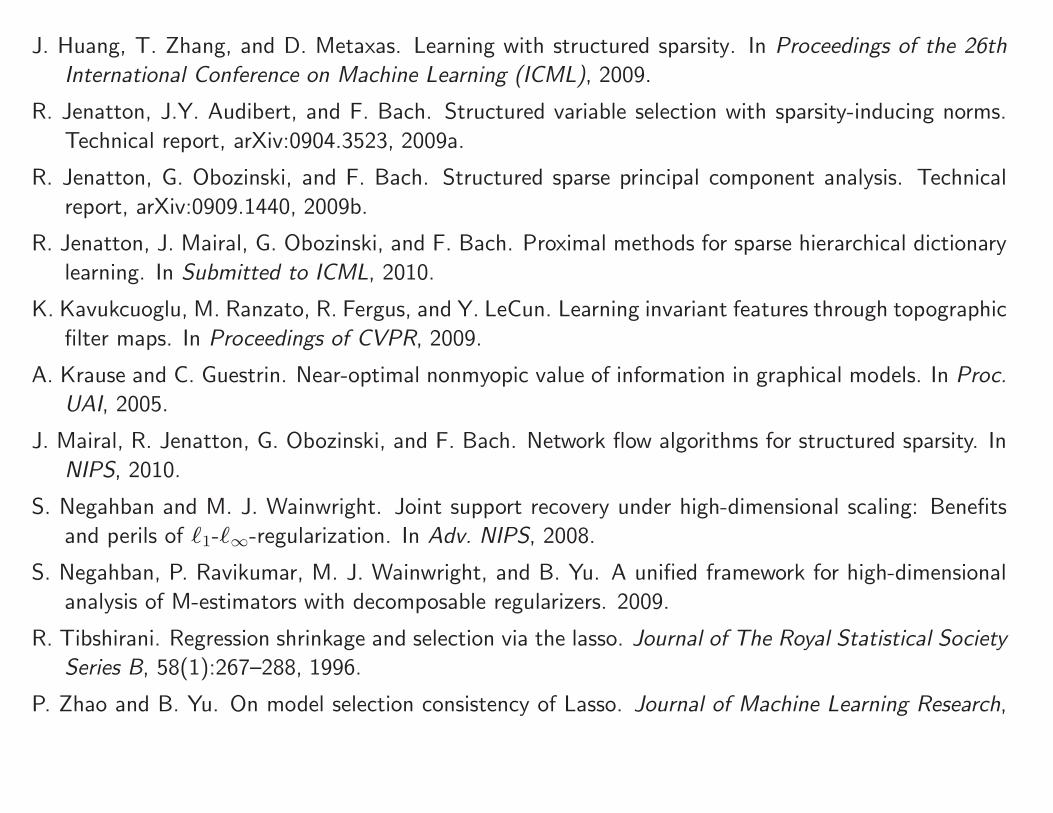
Structured sparse PCA (Jenatton et al., 2009b)
raw data Structured sparse PCA
• Enforce selection of convex nonzero patterns ⇒ robustness to
occlusion in face identification
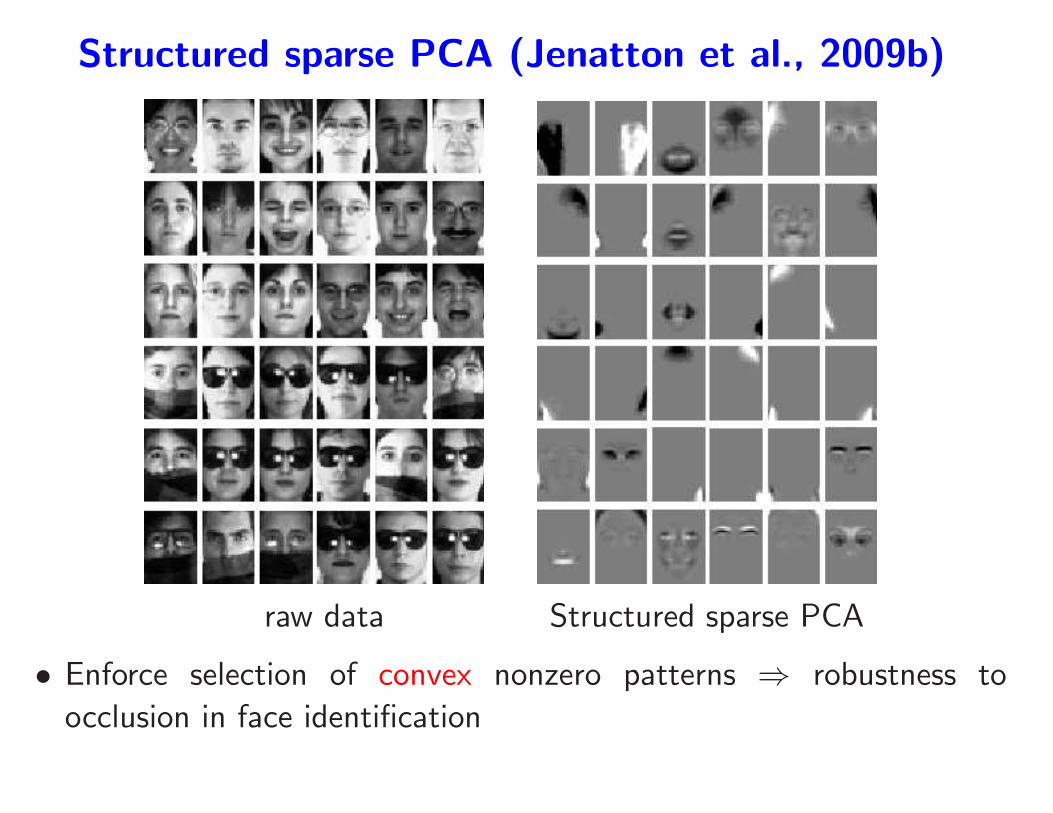
Structured sparse PCA (Jenatton et al., 2009b)
raw data Structured sparse PCA
• Enforce selection of convex nonzero patterns ⇒ robustness to
occlusion in face identification
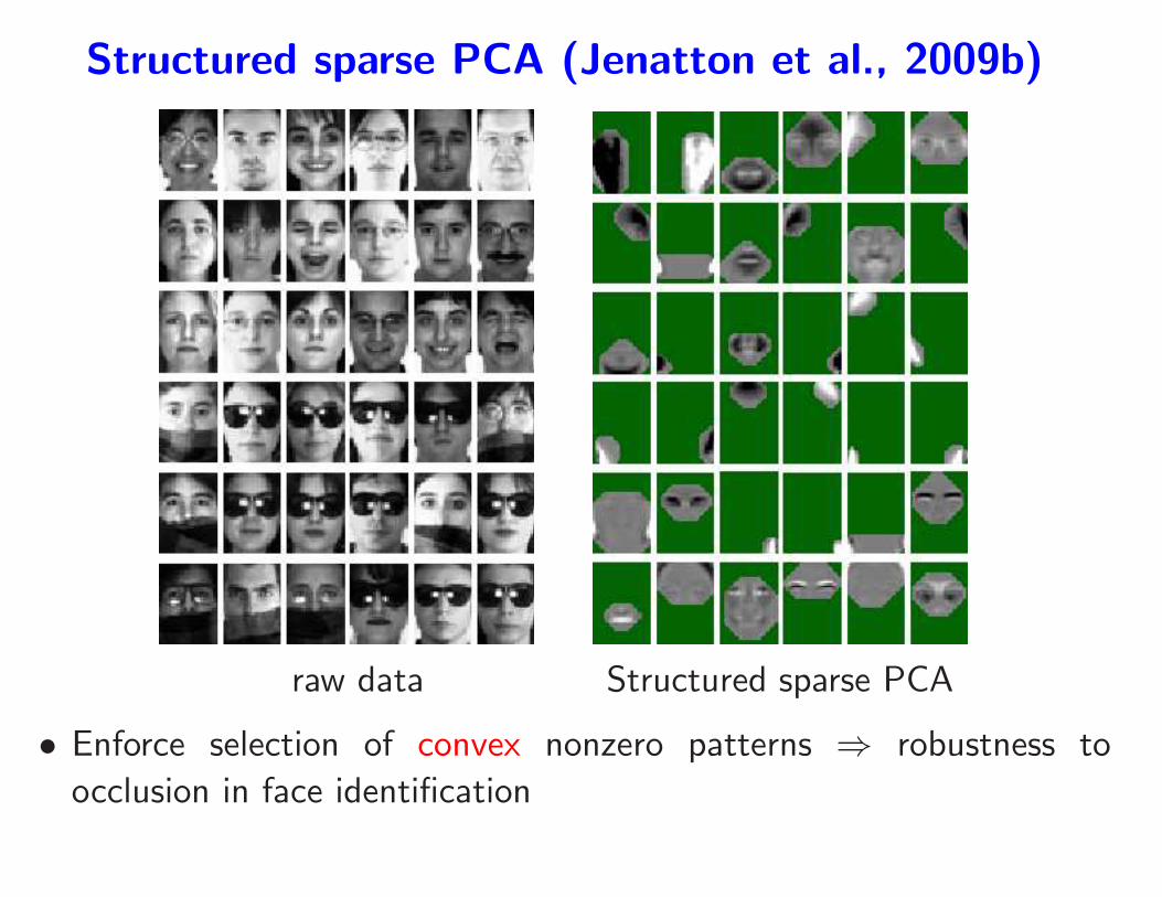
Selection of contiguous patterns in a sequence
• G is the set of blue groups: any union of blue groups set to zero
leads to the selection of a contiguous pattern
•∑
G∈G ‖wG‖∞ ⇒ F (A) = p− 2 + Range(A) if A 6= ∅, F (∅) = 0
– Jump from 0 to p− 1: tends to include all variables simultaneously
– Add ν|A| to smooth the kink: all sparsity patterns are possible
– Contiguous patterns are favored (and not forced)
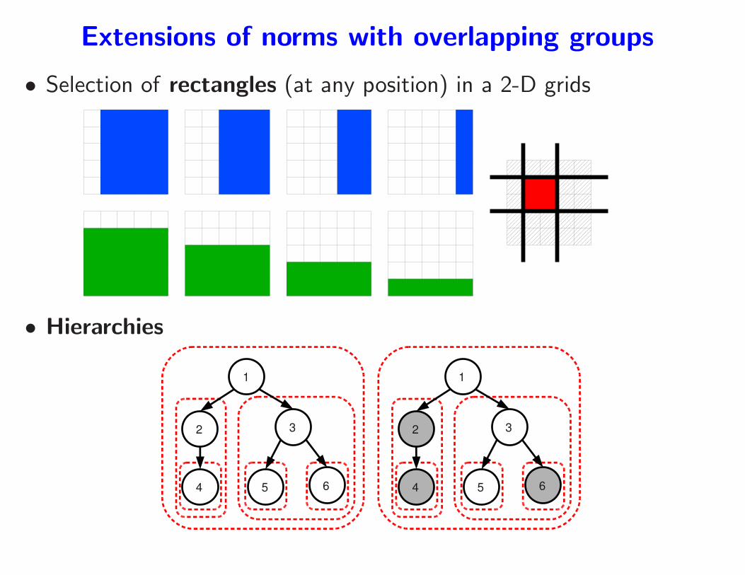
Extensions of norms with overlapping groups
• Selection of rectangles (at any position) in a 2-D grids
• Hierarchies
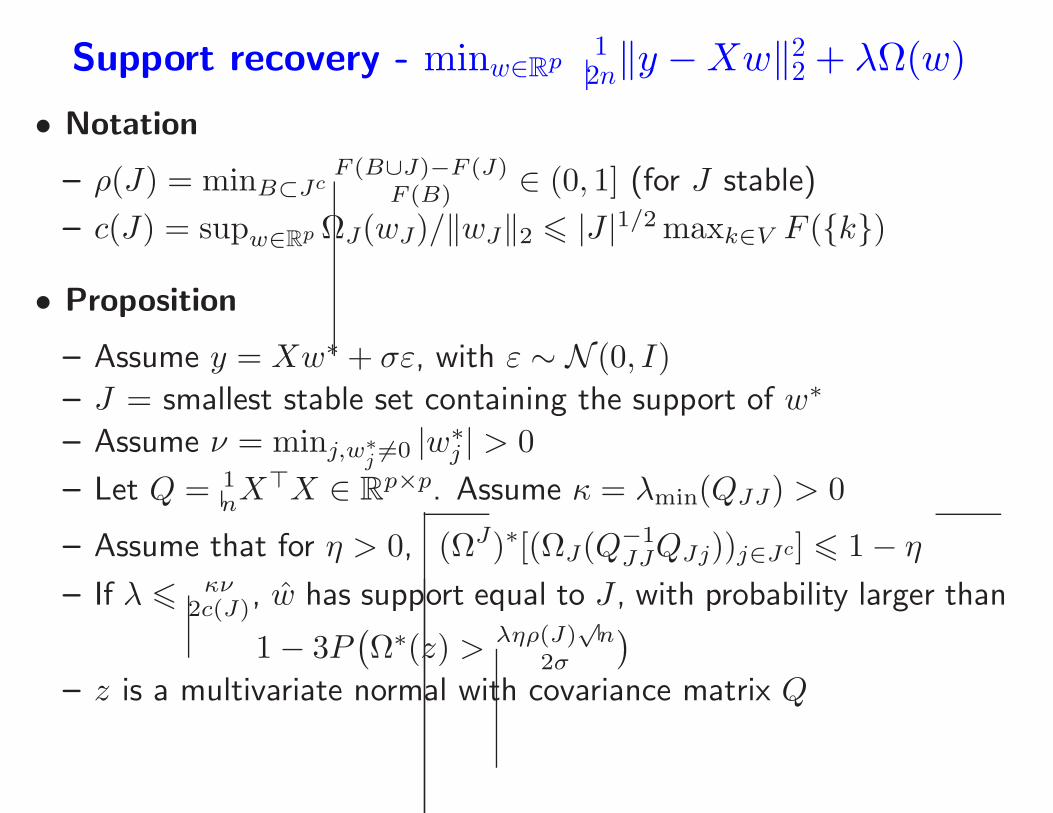
Support recovery - minw∈Rp12n‖y −Xw‖22 + λΩ(w)
• Notation
– ρ(J) = minB⊂JcF (B∪J)−F (J)
F (B) ∈ (0, 1] (for J stable)
– c(J) = supw∈Rp ΩJ(wJ)/‖wJ‖2 6 |J |1/2maxk∈V F (k)
• Proposition
– Assume y = Xw∗ + σε, with ε ∼ N (0, I)
– J = smallest stable set containing the support of w∗
– Assume ν = minj,w∗j 6=0 |w
∗j | > 0
– Let Q = 1nX
⊤X ∈ Rp×p. Assume κ = λmin(QJJ) > 0
– Assume that for η > 0, (ΩJ)∗[(ΩJ(Q−1JJQJj))j∈Jc] 6 1− η
– If λ 6κν
2c(J), w has support equal to J , with probability larger than
1− 3P(
Ω∗(z) > ληρ(J)√n
2σ
)
– z is a multivariate normal with covariance matrix Q
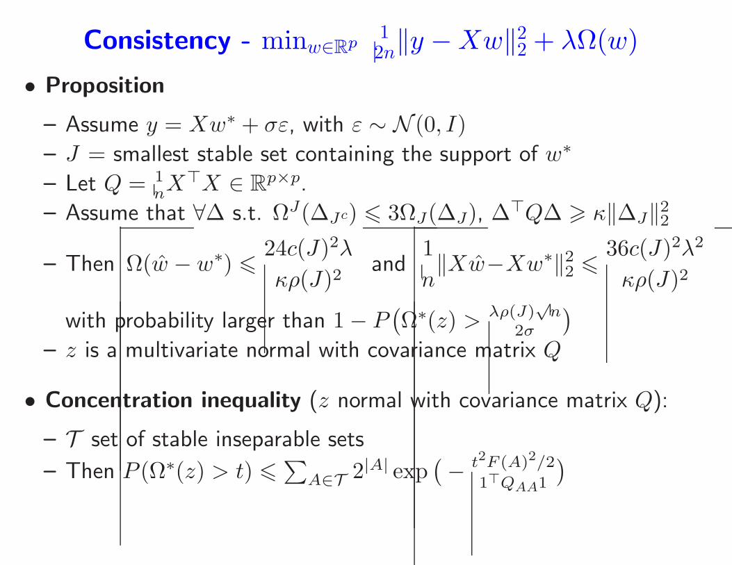
Consistency - minw∈Rp12n‖y −Xw‖22 + λΩ(w)
• Proposition
– Assume y = Xw∗ + σε, with ε ∼ N (0, I)
– J = smallest stable set containing the support of w∗
– Let Q = 1nX
⊤X ∈ Rp×p.
– Assume that ∀∆ s.t. ΩJ(∆Jc) 6 3ΩJ(∆J), ∆⊤Q∆ > κ‖∆J‖
22
– Then Ω(w − w∗) 624c(J)2λ
κρ(J)2and
1
n‖Xw−Xw∗‖22 6
36c(J)2λ2
κρ(J)2
with probability larger than 1− P(
Ω∗(z) > λρ(J)√n
2σ
)
– z is a multivariate normal with covariance matrix Q
• Concentration inequality (z normal with covariance matrix Q):
– T set of stable inseparable sets
– Then P (Ω∗(z) > t) 6∑
A∈T 2|A| exp(
− t2F (A)2/2
1⊤QAA1
)


![Submodular Optimization with Submodular Cover and ... · discrete optimization problems. For example the Submodular Set Cover problem (henceforth SSC) [47] occurs as a special case](https://img.pdfslide.net/doc/110x75/5cdba12d88c993a6778d0d6d/submodular-optimization-with-submodular-cover-and-discrete-optimization.jpg)