Embed Size (px)
Citation preview
Structures in the Dynamical Plane
Dynamics of the family of complex maps
Paul BlanchardToni GarijoMatt HolzerDan LookSebastian Marotta Mark Morabito
with:
€
Fλ (z) = zn +λ
zn
Monica Moreno RochaKevin PilgrimElizabeth RussellYakov ShapiroDavid UminskySum Wun Ellce
, n > 1

1. Dynamic classsification of escape time Sierpinski curve Julia sets
3. Cantor necklaces in the dynamical plane
2. Julia sets converging to the unit disk
4. Internal rays
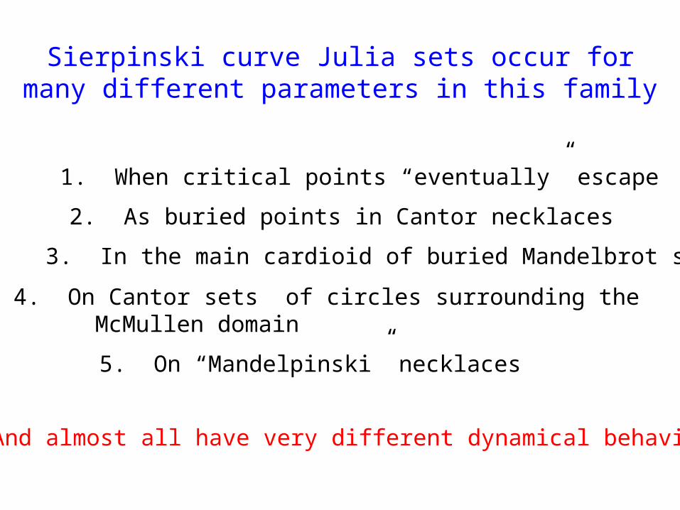
Sierpinski curve Julia sets occur formany different parameters in this family
1. When critical points “eventually” escape
2. As buried points in Cantor necklaces
3. In the main cardioid of buried Mandelbrot sets
4. On Cantor sets of circles surrounding the McMullen domain
5. On “Mandelpinski” necklaces
And almost all have very different dynamical behavior

QuickTime™ and aTIFF (LZW) decompressor
are needed to see this picture.
QuickTime™ and aTIFF (LZW) decompressor
are needed to see this picture.
QuickTime™ and aTIFF (LZW) decompressor
are needed to see this picture.
Sierpinski curve Julia sets occur formany different parameters in this family
All these sets are homeomorphic, but the dynamics on each are very different

A Sierpinski curve is any planar set that is homeomorphic to the Sierpinski carpet fractal.
QuickTime™ and aTIFF (LZW) decompressor
are needed to see this picture.
The Sierpinski Carpet
Recall:

QuickTime™ and aTIFF (LZW) decompressor
are needed to see this picture.
The Sierpinski Carpet
Topological Characterization
Any planar set that is:
1. compact2. connected3. locally connected4. nowhere dense5. any two complementary domains are bounded by simple closed curves that are pairwise disjoint
is a Sierpinski curve.

QuickTime™ and aTIFF (LZW) decompressor
are needed to see this picture.
€
λ = 0
€
Fλ
( z ) = z2
+λ
z2
When , the Julia set is the unit circle
€
λ = 0

QuickTime™ and aTIFF (LZW) decompressor
are needed to see this picture.
€
λ = 0
€
Fλ
( z ) = z2
+λ
z2
€
λ ≠ 0
€
λ = −1 / 16
QuickTime™ and aTIFF (LZW) decompressor
are needed to see this picture.
But when , theJulia set explodes
A Sierpinski curve
When , the Julia set is the unit circle
€
λ = 0

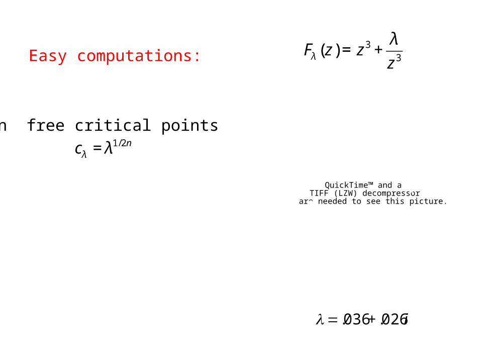
Easy computations:
QuickTime™ and aTIFF (LZW) decompressor
are needed to see this picture.
€
Fλ (z ) = z 3 +λ
z 3
€
λ=.036+.026i
2n free critical points
€
cλ = λ1/2n
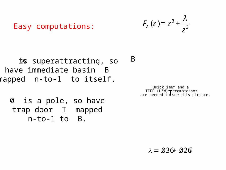
Easy computations:
QuickTime™ and aTIFF (LZW) decompressor
are needed to see this picture.
€
λ=.036+.026i
2n free critical points
€
cλ = λ1/2n€
Fλ (z ) = z 3 +λ
z 3

Easy computations:
QuickTime™ and aTIFF (LZW) decompressor
are needed to see this picture.
€
λ=.036+.026i
2n free critical points
€
cλ = λ1/2n
Only 2 critical values
€
vλ = ±2 λ
€
Fλ (z ) = z 3 +λ
z 3

Easy computations:
QuickTime™ and aTIFF (LZW) decompressor
are needed to see this picture.
€
λ=.036+.026i
2n free critical points
€
cλ = λ1/2n
Only 2 critical values
€
vλ = ±2 λ
€
Fλ (z ) = z 3 +λ
z 3

Easy computations:
QuickTime™ and aTIFF (LZW) decompressor
are needed to see this picture.
€
λ=.036+.026i
2n free critical points
€
cλ = λ1/2n
Only 2 critical values
€
vλ = ±2 λ
€
Fλ (z ) = z 3 +λ
z 3

Easy computations:
QuickTime™ and aTIFF (LZW) decompressor
are needed to see this picture.
€
λ=.036+.026i
2n free critical points
€
cλ = λ1/2n
Only 2 critical values
€
vλ = ±2 λ
€
Fλ (z ) = z 3 +λ
z 3

Easy computations:
€
λ=.036+.026i
2n free critical points
€
cλ = λ1/2n
Only 2 critical values
€
vλ = ±2 λ
But really only one free critical orbit
€
Fλ (z ) = z 3 +λ
z 3
QuickTime™ and aTIFF (LZW) decompressor
are needed to see this picture.

Easy computations:
€
λ=.036+.026i
2n free critical points
€
cλ = λ1/2n
Only 2 critical values
€
vλ = ±2 λ
€
Fλ (z ) = z 3 +λ
z 3
QuickTime™ and aTIFF (LZW) decompressor
are needed to see this picture.
And J has 2n-fold symmetry
But really only one free critical orbit

Easy computations:
QuickTime™ and aTIFF (LZW) decompressor
are needed to see this picture.
€
λ=.036+.026i
is superattracting, so have immediate basin Bmapped n-to-1 to itself.
B€
Fλ (z ) = z 3 +λ
z 3
€
∞
Easy computations:
QuickTime™ and aTIFF (LZW) decompressor
are needed to see this picture.
€
λ=.036+.026i
is superattracting, so have immediate basin Bmapped n-to-1 to itself.
B
T
€
Fλ (z ) = z 3 +λ
z 3
€
∞
0 is a pole, so havetrap door T mapped
n-to-1 to B.

Easy computations:
QuickTime™ and aTIFF (LZW) decompressor
are needed to see this picture.
€
λ=.036+.026i
is superattracting, so have immediate basin Bmapped n-to-1 to itself.
B
T
€
Fλ (z ) = z 3 +λ
z 3
€
∞
So any orbit that eventuallyenters B must do so by
passing through T.
0 is a pole, so havetrap door T mapped
n-to-1 to B.

The Escape Trichotomy
€
vλ∈
€
J ( Fλ
)
€
⇒B is a Cantor set
T
€
vλ∈ is a Cantor set of
simple closed curves
€
J ( Fλ
)
€
Fλ
k(v
λ) ∈ T
€
J ( Fλ
) is a Sierpinski curve
There are three distinct ways the critical orbit can enter B:
(this case does not occur if n = 2)
€
⇒
€
⇒
(McMullen)

QuickTime™ and aTIFF (LZW) decompressor
are needed to see this picture.
QuickTime™ and aTIFF (LZW) decompressor
are needed to see this picture.
€
vλ∈
€
J ( Fλ
)
€
⇒B is a Cantor set
parameter planewhen n = 3
J is a Cantor set
€
λ

QuickTime™ and aTIFF (LZW) decompressor
are needed to see this picture.
€
vλ∈
€
⇒T
parameter planewhen n = 3
J is a Cantor set of simple closed curves
€
λ lies in the McMullen domain
€
λQuickTime™ and a
TIFF (LZW) decompressorare needed to see this picture.

QuickTime™ and aTIFF (LZW) decompressor
are needed to see this picture.
€
⇒T
parameter planewhen n = 3
€
λ lies in a Sierpinski hole
€
λ
€
Fλ
k(v
λ) ∈
QuickTime™ and aTIFF (LZW) decompressor
are needed to see this picture.
J is an escape time Sierpinski curve
c

Have an exact count of the number of Sierpinski holes:
Theorem (Roesch): Given n, there are exactly (n-1)(2n) Sierpinski holes with escape time k. (k-3)

Have an exact count of the number of Sierpinski holes:
QuickTime™ and aTIFF (LZW) decompressor
are needed to see this picture.
n = 3escape time 32 Sierpinski holes
parameter planen = 3
Theorem (Roesch): Given n, there are exactly (n-1)(2n) Sierpinski holes with escape time k. (k-3)

Have an exact count of the number of Sierpinski holes:
QuickTime™ and aTIFF (LZW) decompressor
are needed to see this picture.
n = 3escape time 412 Sierpinski holes
parameter planen = 3
Theorem (Roesch): Given n, there are exactly (n-1)(2n) Sierpinski holes with escape time k. (k-3)

Have an exact count of the number of Sierpinski holes:
n = 4escape time 33 Sierpinski holes
QuickTime™ and aTIFF (LZW) decompressor
are needed to see this picture.
parameter planen = 4
Theorem (Roesch): Given n, there are exactly (n-1)(2n) Sierpinski holes with escape time k. (k-3)

Have an exact count of the number of Sierpinski holes:
n = 4escape time 424 Sierpinski holes
QuickTime™ and aTIFF (LZW) decompressor
are needed to see this picture.
parameter planen = 4
Theorem (Roesch): Given n, there are exactly (n-1)(2n) Sierpinski holes with escape time k. (k-3)

Have an exact count of the number of Sierpinski holes:
n = 4escape time 12 402,653,184 Sierpinski holes
QuickTime™ and aTIFF (LZW) decompressor
are needed to see this picture.
Guess what? I again forgot to indicate their locations. parameter plane
n = 4
Theorem (Roesch): Given n, there are exactly (n-1)(2n) Sierpinski holes with escape time k. (k-3)

Given two Sierpinski curve Julia sets, when do we know that the dynamics on them are the same, i.e., the maps are conjugate on the Julia sets?
Main Question:
QuickTime™ and aTIFF (LZW) decompressor
are needed to see this picture.
QuickTime™ and aTIFF (LZW) decompressor
are needed to see this picture.
Part 1: Dynamic Classification of Escape Time Sierpinski Curve Julia sets

#1: If and are drawn from the same Sierpinski hole, then the correspondingmaps have the same dynamics, i.e., they are topologically conjugate on their Julia sets.€
λ
€
μ
QuickTime™ and aTIFF (LZW) decompressor
are needed to see this picture.
parameter planen = 4

#1: If and are drawn from the same Sierpinski hole, then the correspondingmaps have the same dynamics, i.e., they are topologically conjugate on their Julia sets.
QuickTime™ and aTIFF (LZW) decompressor
are needed to see this picture.So all these parametershave the same dynamicson their Julia sets.
parameter planen = 4
€
λ
€
μ

#1: If and are drawn from the same Sierpinski hole, then the correspondingmaps have the same dynamics, i.e., they are topologically conjugate on their Julia sets.€
λ
€
μ
QuickTime™ and aTIFF (LZW) decompressor
are needed to see this picture.
parameter planen = 4
This uses quasiconformalsurgery techniques
#1: If and are drawn from the same Sierpinski hole, then the correspondingmaps have the same dynamics, i.e., they are topologically conjugate on their Julia sets.€
λ
€
μ
#2: If these parameters come from Sierpinski holes with different “escape times,” then the maps cannot be conjugate.

QuickTime™ and aTIFF (LZW) decompressor
are needed to see this picture.
QuickTime™ and aTIFF (LZW) decompressor
are needed to see this picture.
€
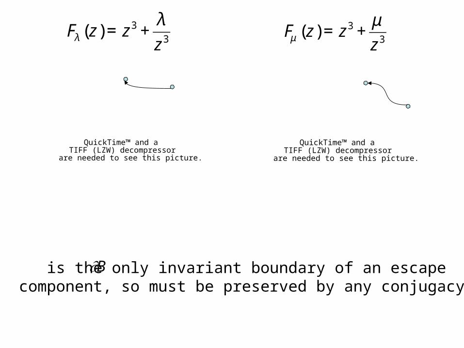
Fλ (z ) = z 3 +λ
z 3
Two Sierpinski curve Julia sets, so they are homeomorphic.
€
cλ
€
cμ
€
Fμ (z ) = z 3 +μ
z 3

QuickTime™ and aTIFF (LZW) decompressor
are needed to see this picture.
QuickTime™ and aTIFF (LZW) decompressor
are needed to see this picture.
escape time 3 escape time 4
So these maps cannot be topologically conjugate.
€
cλ
€
cμ
€
Fλ (z ) = z 3 +λ
z 3
€
Fμ (z ) = z 3 +μ
z 3
QuickTime™ and aTIFF (LZW) decompressor
are needed to see this picture.
QuickTime™ and aTIFF (LZW) decompressor
are needed to see this picture.
is the only invariant boundary of an escapecomponent, so must be preserved by any conjugacy.
€
∂B
€
Fλ (z ) = z 3 +λ
z 3
€
Fμ (z ) = z 3 +μ
z 3

QuickTime™ and aTIFF (LZW) decompressor
are needed to see this picture.
QuickTime™ and aTIFF (LZW) decompressor
are needed to see this picture.
is the only preimage of , so this curve must also be preserved by a conjugacy.
€
∂B
€
∂T
€
Fλ (z ) = z 3 +λ
z 3
€
Fμ (z ) = z 3 +μ
z 3

QuickTime™ and aTIFF (LZW) decompressor
are needed to see this picture.
QuickTime™ and aTIFF (LZW) decompressor
are needed to see this picture.
If a boundary component is mapped toafter k iterations, its image under the conjugacy must also have this property,and so forth..... €
∂T
€
Fλ (z ) = z 3 +λ
z 3
€
Fμ (z ) = z 3 +μ
z 3

QuickTime™ and aTIFF (LZW) decompressor
are needed to see this picture.
2-11-1
3-1
The curves around c are special; they are the only boundary curvesin J mapped 2-1 onto their images.
c
€
Fλ (z ) = z 3 +λ
z 3

QuickTime™ and aTIFF (LZW) decompressor
are needed to see this picture.
QuickTime™ and aTIFF (LZW) decompressor
are needed to see this picture.
2-11-1
3-1
2-1
3-11-11-1
This bounding region takes 3 iterates to land on the
boundary of B.
But this bounding region takes 4 iterates to land, so
these maps are not conjugate.
€
Fλ (z ) = z 3 +λ
z 3
€
Fμ (z ) = z 3 +μ
z 3
For this it suffices to consider the centers of the Sierpinski holes; i.e., parameter values
for which for some k 3.
€
Fλk(cλ ) = ∞
#3: What if two maps lie in different Sierpinski holes that have the same escape time?

#3: What if two maps lie in different Sierpinski holes that have the same escape time?
For this it suffices to consider the centers of the Sierpinski holes; i.e., parameter values
for which for some k 3.
Two such centers of Sierpinski holes are “critically finite” maps, so by Thurston’s Theorem, if they are topologically
conjugate in the plane, they can be conjugated by a Mobius transformation (in the orientation preserving case).
€
Fλk(cλ ) = ∞

#3: What if two maps lie in different Sierpinski holes that have the same escape time?
For this it suffices to consider the centers of the Sierpinski holes; i.e., parameter values
for which for some k 3.
Two such centers of Sierpinski holes are “critically finite” maps, so by Thurston’s Theorem, if they are topologically
conjugate in the plane, they can be conjugated by a Mobius transformation (in the orientation preserving case).
Since and under the conjugacy,the Mobius conjugacy must be of the form .
€
∞→ ∞
€
0 → 0
€
z →α z
€
Fλk(cλ ) = ∞

€
h(Fλ (z)) = Fμ (h(z))then:
€
α zn +λ
zn
⎛
⎝ ⎜
⎞
⎠ ⎟=αzn +
αλ
zn=α nzn +
μ
α nzn
If we have a conjugacy
€
h(z) = α z

If we have a conjugacy
€
h(Fλ (z)) = Fμ (h(z))then:
€
α zn +λ
zn
⎛
⎝ ⎜
⎞
⎠ ⎟=αzn +
αλ
zn=α nzn +
μ
α nzn
Comparing coefficients:
€
αn−1 =1
€
h(z) = α z

€
h(Fλ (z)) = Fμ (h(z))then:
€
α zn +λ
zn
⎛
⎝ ⎜
⎞
⎠ ⎟=αzn +
αλ
zn=α nzn +
μ
α nzn
Comparing coefficients:
€
αn−1 =1
€
μ =α2λ
If we have a conjugacy
€
h(z) = α z

€
h(Fλ (z)) = Fμ (h(z))then:
€
α zn +λ
zn
⎛
⎝ ⎜
⎞
⎠ ⎟=αzn +
αλ
zn=α nzn +
μ
α nzn
Comparing coefficients:
€
αn−1 =1
€
μ =α2λ
Easy check --- for the orientation reversing case:
is conjugate to via
€
Fλ
€
Fλ
€
h(z) = z
If we have a conjugacy
€
h(z) = α z

Theorem. If and are centers of Sierpinski holes, then iff or whereis a primitive root of unity; then any twoparameters drawn from these holes have the samedynamics. (with K. Pilgrim)
€
Fλ ≈ Fμ
€
α
€
(n −1)st
€
μ
€
λ
n = 3: Only and are conjugatecenters since
€
λ
€
λ
€
αλ
€
α2λ
€
λ
€
λ
€
αλ
€
α2λ, , , , ,n = 4: Only
are conjugate centers where .
€
α 3 =1
€
μ =α2 jλ
€
μ =α2 jλ
€
α =−1

QuickTime™ and aTIFF (LZW) decompressor
are needed to see this picture.
n = 3, escape time 4, 12 Sierpinski holes,but only six conjugacy classes
€
λ
€
λconjugate centers: ,

QuickTime™ and aTIFF (LZW) decompressor
are needed to see this picture.
n = 3, escape time 4, 12 Sierpinski holes,but only six conjugacy classes
€
λ
€
λconjugate centers: ,

QuickTime™ and aTIFF (LZW) decompressor
are needed to see this picture.
n = 3, escape time 4, 12 Sierpinski holes,but only six conjugacy classes
€
λ
€
λconjugate centers: ,

QuickTime™ and aTIFF (LZW) decompressor
are needed to see this picture.
n = 3, escape time 4, 12 Sierpinski holes,but only six conjugacy classes
€
λ
€
λconjugate centers: ,

QuickTime™ and aTIFF (LZW) decompressor
are needed to see this picture.
€
αλ
€
α2λ
€
λ
€
λ
€
αλ
€
α2λ, , , , , where
€
α 3 =1
n = 4, escape time 4, 24 Sierpinski holes,but only five conjugacy classes
conjugate centers:

QuickTime™ and aTIFF (LZW) decompressor
are needed to see this picture.
€
αλ
€
α2λ
€
λ
€
λ
€
αλ
€
α2λ, , , , , where
€
α 3 =1
n = 4, escape time 4, 24 Sierpinski holes,but only five conjugacy classes
conjugate centers:

QuickTime™ and aTIFF (LZW) decompressor
are needed to see this picture.
€
αλ
€
α2λ
€
λ
€
λ
€
αλ
€
α2λ, , , , , where
€
α 3 =1
n = 4, escape time 4, 24 Sierpinski holes,but only five conjugacy classes
conjugate centers:

QuickTime™ and aTIFF (LZW) decompressor
are needed to see this picture.
€
αλ
€
α2λ
€
λ
€
λ
€
αλ
€
α2λ, , , , , where
€
α 3 =1
n = 4, escape time 4, 24 Sierpinski holes,but only five conjugacy classes
conjugate centers:

QuickTime™ and aTIFF (LZW) decompressor
are needed to see this picture.
€
αλ
€
α2λ
€
λ
€
λ
€
αλ
€
α2λ, , , , , where
€
α 3 =1
n = 4, escape time 4, 24 Sierpinski holes,but only five conjugacy classes
conjugate centers:

Theorem: For any n there are exactly (n-1) (2n) Sierpinski holes with escape time k. The number ofdistinct conjugacy classes is given by:
k-3
a. (2n) when n is odd;k-3
b. (2n) /2 + 2 when n is even.k-3 k-4

QuickTime™ and aTIFF (LZW) decompressor
are needed to see this picture.
QuickTime™ and aTIFF (LZW) decompressor
are needed to see this picture.
For n odd, there are no Sierpinski holes along the real axis,so there are exactly n - 1 conjugate Sierpinski holes.
n = 3 n = 5

n = 4
QuickTime™ and aTIFF (LZW) decompressor
are needed to see this picture.
For n even, there is a “Cantor necklace” along the negativeaxis, so there are some “real” Sierpinski holes,

For n even, there is a “Cantor necklace” along the negativeaxis, so there are some “real” Sierpinski holes,
n = 4
QuickTime™ and aTIFF (LZW) decompressor
are needed to see this picture.

For n even, there is a “Cantor necklace” along the negativeaxis, so there are some “real” Sierpinski holes,
n = 4 magnification
QuickTime™ and aTIFF (LZW) decompressor
are needed to see this picture.
QuickTime™ and aTIFF (LZW) decompressor
are needed to see this picture. M

For n even, there is a “Cantor necklace” along the negativeaxis, so there are some “real” Sierpinski holes,
n = 4 magnification
QuickTime™ and aTIFF (LZW) decompressor
are needed to see this picture.
QuickTime™ and aTIFF (LZW) decompressor
are needed to see this picture. M3

For n even, there is a “Cantor necklace” along the negativeaxis, so there are some “real” Sierpinski holes,
n = 4 magnification
QuickTime™ and aTIFF (LZW) decompressor
are needed to see this picture.
QuickTime™ and aTIFF (LZW) decompressor
are needed to see this picture. M34 4

For n even, there is a “Cantor necklace” along the negativeaxis, so there are some “real” Sierpinski holes,
n = 4 magnification
QuickTime™ and aTIFF (LZW) decompressor
are needed to see this picture.
QuickTime™ and aTIFF (LZW) decompressor
are needed to see this picture. M34 4
5 5

For n even, there is a “Cantor necklace” along the negativeaxis, so we can count the number of “real” Sierpinski holes,
and there are exactly n - 1 conjugate holes in this case:
n = 4 magnification
QuickTime™ and aTIFF (LZW) decompressor
are needed to see this picture.
QuickTime™ and aTIFF (LZW) decompressor
are needed to see this picture. M34 4
5 5

For n even, there are also 2(n - 1) “complex” Sierpinski holes that have conjugate dynamics:
n = 4 magnification
QuickTime™ and aTIFF (LZW) decompressor
are needed to see this picture.
QuickTime™ and aTIFF (LZW) decompressor
are needed to see this picture. M

QuickTime™ and aTIFF (LZW) decompressor
are needed to see this picture.
n = 4: 402,653,184 Sierpinski holes with escape time 12; 67,108,832 distinct conjugacy classes.
Will someone please remind me to
indicate their locations?

QuickTime™ and aTIFF (LZW) decompressor
are needed to see this picture.
n = 4: 402,653,184 Sierpinski holes with escape time 12; 67,108,832 distinct conjugacy classes.
Problem: use symbolic dynamics to describe these conjugacy classes.

Part 2: Julia sets converging to the unit disk
With Toni Garijo

n = 2: When , the Julia set of is the unit circle. But, as , the Julia set of converges to the closed unit disk
€
Fλ
€
λ → 0
€
λ =0
€
Fλ
Part 2: Julia sets converging to the unit disk
With Toni Garijo

n = 2: When , the Julia set of is the unit circle. But, as , the Julia set of converges to the closed unit disk
€
Fλ
€
λ → 0
€
λ =0
€
Fλ
n > 2: J is always a Cantor set of “circles” when is small.
€
λ
Part 2: Julia sets converging to the unit disk
With Toni Garijo
n > 2: J is always a Cantor set of “circles” when is small.
n = 2: When , the Julia set of is the unit circle. But, as , the Julia set of converges to the closed unit disk
€
Fλ
€
λ → 0
€
λ =0
€
Fλ
Moreover, there is a such that there is always a“round” annulus of “thickness” between two of these circles in the Fatou set. So J does not converge to the unit disk when n > 2.
€
λ
€
δ > 0
€
δ
Part 2: Julia sets converging to the unit disk
With Toni Garijo

n = 2
Theorem: When n = 2, the Julia sets converge to the unit disk as
QuickTime™ and aTIFF (LZW) decompressor
are needed to see this picture.
€
λ → 0
Suppose the Julia sets do not converge to the unit disk D as
€
λ → 0
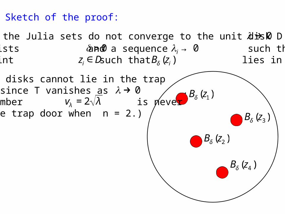
Sketch of the proof:

Suppose the Julia sets do not converge to the unit disk D as
€
λ → 0
Sketch of the proof:
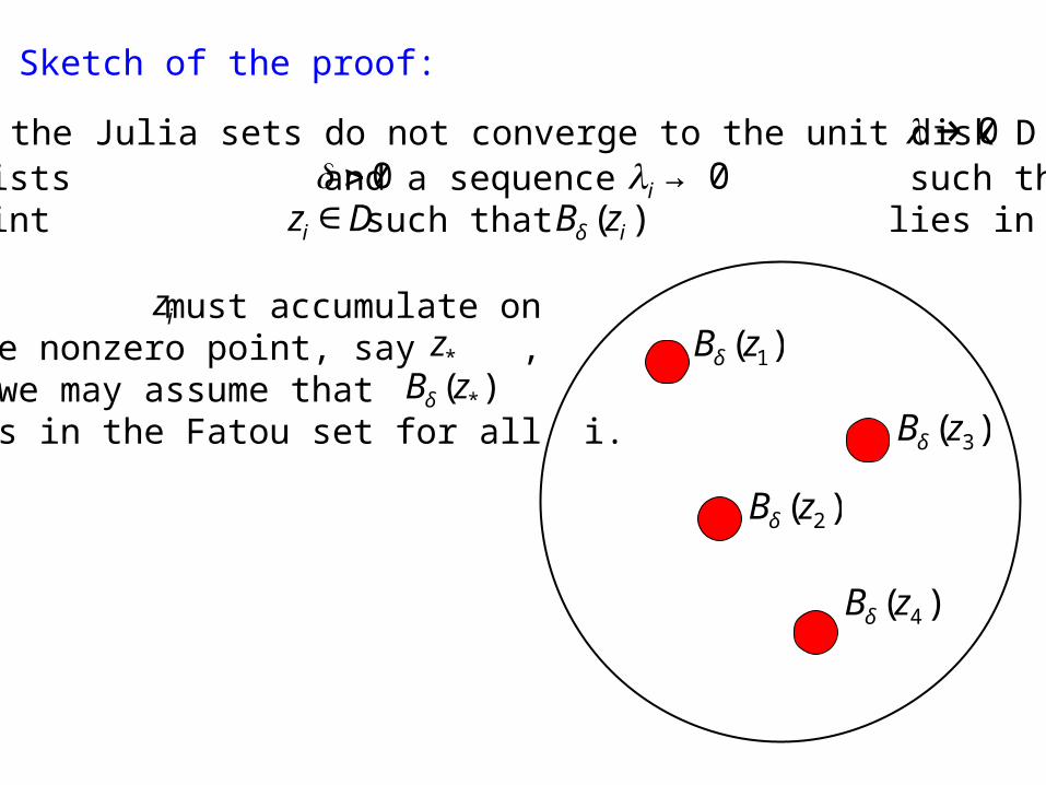
Then there exists and a sequence such that, for each i,there is a point such that lies in the Fatou set.
€
Bδ (zi )
€
δ > 0
€
λi → 0
€
zi ∈D

Suppose the Julia sets do not converge to the unit disk D as
€
λ → 0
Sketch of the proof:
Then there exists and a sequence such that, for each i,there is a point such that lies in the Fatou set.
€
Bδ (zi )
€
λi → 0
€
zi ∈D
€
Bδ (z1)
€
Bδ (z2 )
€
Bδ (z3)
€
Bδ (z4 )
€
δ > 0
Suppose the Julia sets do not converge to the unit disk D as
€
λ → 0
Sketch of the proof:
Then there exists and a sequence such that, for each i,there is a point such that lies in the Fatou set.
€
Bδ (zi )
€
λi → 0
€
zi ∈D
€
Bδ (z1)
€
Bδ (z2 )
€
Bδ (z3)
€
Bδ (z4 )
€
δ > 0
These disks cannot lie in the trapdoor since T vanishes as .(Remember is never in the trap door when n = 2.)
€
λ → 0
€
vλ = 2 λ
Suppose the Julia sets do not converge to the unit disk D as
€
λ → 0
Sketch of the proof:
Then there exists and a sequence such that, for each i,there is a point such that lies in the Fatou set.
€
Bδ (zi )
€
λi → 0
€
zi ∈D
The must accumulate on some nonzero point, say ,so we may assume that lies in the Fatou set for all i.
€
zi
€
z*
€
Bδ (z*)
€
Bδ (z1)
€
Bδ (z2 )
€
Bδ (z3)
€
Bδ (z4 )
€
δ > 0

Suppose the Julia sets do not converge to the unit disk D as
€
λ → 0
Sketch of the proof:
Then there exists and a sequence such that, for each i,there is a point such that lies in the Fatou set.
€
Bδ (zi )
€
λi → 0
€
zi ∈D
€
Bδ (z*)
The must accumulate on some nonzero point, say ,so we may assume that lies in the Fatou set for all i.
€
zi
€
z*€
δ > 0
€
Bδ (z*)

Suppose the Julia sets do not converge to the unit disk D as
€
λ → 0
Sketch of the proof:
Then there exists and a sequence such that, for each i,there is a point such that lies in the Fatou set.
€
Bδ (zi )
€
λi → 0
€
zi ∈D
€
Bδ (z*)
The must accumulate on some nonzero point, say ,so we may assume that lies in the Fatou set for all i.
€
zi
€
z*
But for large i, so stretchesinto an “annulus” that surrounds the origin, so thisdisconnects the Julia set.€
Fλ i≈ z2
€
Fλ i
k
€
Bδ (z*)€
Fλk
€
δ > 0
€
Bδ (z*)

So the Fatou components must become arbitrarily small:
QuickTime™ and aTIFF (LZW) decompressor
are needed to see this picture.
QuickTime™ and aTIFF (LZW) decompressor
are needed to see this picture.
€
λ =−0.0001
€
λ =−0.0000001

QuickTime™ and aTIFF (LZW) decompressor
are needed to see this picture.
QuickTime™ and aTIFF (LZW) decompressor
are needed to see this picture.
€
λ =.01
QuickTime™ and aTIFF (LZW) decompressor
are needed to see this picture.
€
λ =.0001
€
λ =.000001
n > 2: Note the “round” annuli in the Fatou set; there is alwayssuch an annulus of some fixed width for small.
QuickTime™ and aTIFF (LZW) decompressor
are needed to see this picture.
QuickTime™ and aTIFF (LZW) decompressor
are needed to see this picture.
€
λ =.00000001
€
λ =.0000000001
€
| λ |
QuickTime™ and aTIFF (LZW) decompressor
are needed to see this picture.
€
λ =.000000000001

T
B
€
| λ | small
€
⇒ T is tiny
A0
mod A0 = m is huge
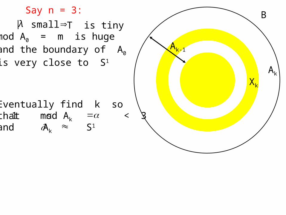
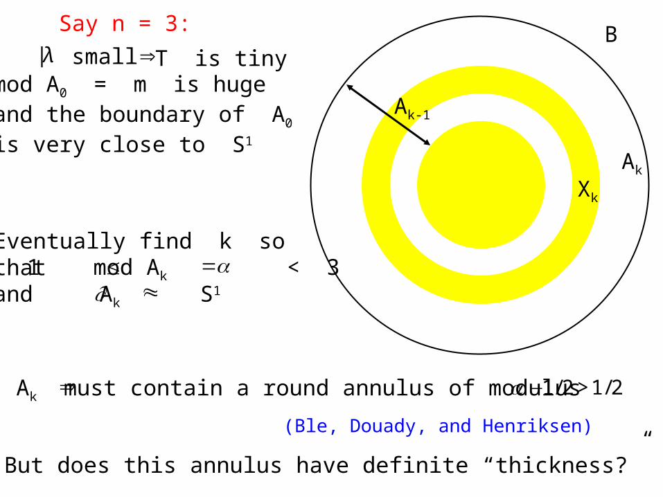
Say n = 3:

T
B
€
| λ | small
€
⇒ T is tiny
A0
mod A0 = m is hugeand the boundary of A0
is very close to S1
Say n = 3:

T
B
€
| λ | small
€
⇒ T is tinymod A0 = m is hugeand the boundary of A0
is very close to S1
Say n = 3:
X1
A1
A1 and A1 mapped to A0;X1 is mapped to T
X1
A1
A1
~~
A0
mod A1 = mod A1 = mod X1 = m/3; A1 S1
€
⇒
€
≈
€
∂~

T
B
€
| λ | small
€
⇒ T is tinymod A0 = m is hugeand the boundary of A0
is very close to S1
Say n = 3:
X1
A1
A1 and A1 mapped to A0;X1 is mapped to T
X2
A1
A2
A2 is mapped to A1;X2 is mapped to X1
mod A2 = mod X2 = m/32; A2 S1
€
⇒mod A1 = mod A1 = mod X1 = m/3; A1 S1
€
⇒
€
≈
€
∂
€
≈
€
∂
~
~

B
€
| λ | small
€
⇒ T is tinymod A0 = m is hugeand the boundary of A0
is very close to S1
Say n = 3:
A1 and A1 mapped to A0;X1 is mapped to T
Xk
Ak
Ak-1
€
M
Ak is mapped to Ak-1; Xk to Xk-1
mod A2 = mod X2 = m/32; A2 S1
€
⇒mod A1 = mod A1 = mod X1 = m/3; A1 S1
~
€
⇒
€
≈
€
∂
€
≈
€
∂mod Ak = mod Xk = m/3k; Ak S1
€
⇒
€
≈
€
∂
A2 is mapped to A1;X2 is mapped to X1
~
€
N
B
€
| λ | small
€
⇒ T is tinymod A0 = m is hugeand the boundary of A0
is very close to S1
Say n = 3:
Xk
Ak
Ak-1
1 mod Ak < 3
€
≤Eventually find k sothatand Ak S1
€
≈
€
∂
€
=α

B
€
| λ | small
€
⇒ T is tinymod A0 = m is hugeand the boundary of A0
is very close to S1
Say n = 3:
Xk
Ak
Ak-1
1 mod Ak < 3
€
≤Eventually find k sothatand Ak S1
€
≈
€
∂
€
⇒ Ak must contain a round annulus of modulus
(Ble, Douady, and Henriksen)
€
=α
€
α −1/2 >1/2
B
€
| λ | small
€
⇒ T is tinymod A0 = m is hugeand the boundary of A0
is very close to S1
Say n = 3:
Xk
Ak
Ak-1
€
⇒ Ak must contain a round annulus of modulus
(Ble, Douady, and Henriksen)
But does this annulus have definite “thickness?”
1 mod Ak < 3
€
≤Eventually find k sothatand Ak S1
€
≈
€
∂
€
=α
€
α −1/2 >1/2

QuickTime™ and aTIFF (LZW) decompressor
are needed to see this picture.
€
∂Ak in here
€
r = 1− ε
€
r = 1+ ε

QuickTime™ and aTIFF (LZW) decompressor
are needed to see this picture.
€
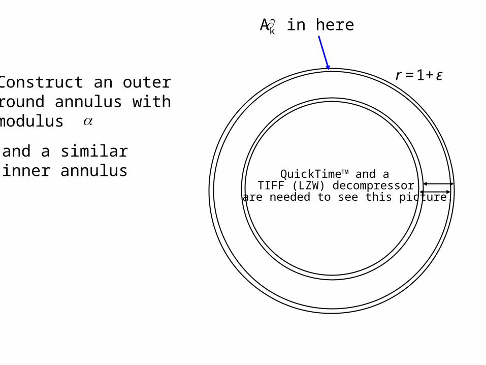
∂Ak in here
€
r = 1+ εConstruct an outerround annulus withmodulus
€
α
QuickTime™ and aTIFF (LZW) decompressor
are needed to see this picture.
€
∂Ak in here
€
r = 1+ εConstruct an outerround annulus withmodulus
€
α
and a similarinner annulus
QuickTime™ and aTIFF (LZW) decompressor
are needed to see this picture.
€
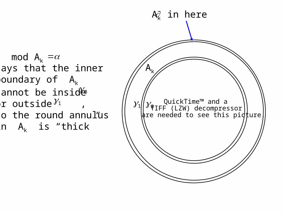
∂Ak in here
€
=αmod Ak
says that the innerboundary of Ak
cannot be insideor outside ,so the round annulusin Ak is “thick”€
γ0
€
γ1
€
γ1
€
γ0
Ak

QuickTime™ and aTIFF (LZW) decompressor
are needed to see this picture.
€
∂Ak in here
€
μ1
€
μ0
Ak
Same argumentsays that Ak Xk
is twice as thick
€
∪
€
∪ Xk

QuickTime™ and aTIFF (LZW) decompressor
are needed to see this picture.
Xk
So Xk musthave definite thickness as well

QuickTime™ and aTIFF (LZW) decompressor
are needed to see this picture.
QuickTime™ and aTIFF (LZW) decompressor
are needed to see this picture.
€
λ =.01
QuickTime™ and aTIFF (LZW) decompressor
are needed to see this picture.
€
λ =.0001
€
λ =.000001
And that’s what we saw earlier: there is always an annulus Xk far out with definite thickness.
QuickTime™ and aTIFF (LZW) decompressor
are needed to see this picture.
QuickTime™ and aTIFF (LZW) decompressor
are needed to see this picture.
€
λ =.00000001
€
λ =.0000000001
QuickTime™ and aTIFF (LZW) decompressor
are needed to see this picture.
€
λ =.000000000001

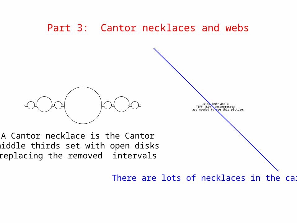
Part 3: Cantor necklaces and webs
A Cantor necklace is the Cantor middle thirds set with open disks replacing the removed intervals.

Part 3: Cantor necklaces and webs
A Cantor necklace is the Cantor middle thirds set with open disks replacing the removed intervals.
QuickTime™ and aTIFF (LZW) decompressor
are needed to see this picture.
Do you see a necklace in the carpet?

Part 3: Cantor necklaces and webs
A Cantor necklace is the Cantor middle thirds set with open disks replacing the removed intervals.
QuickTime™ and aTIFF (LZW) decompressor
are needed to see this picture.
Do you see a necklace in the carpet?

Part 3: Cantor necklaces and webs
A Cantor necklace is the Cantor middle thirds set with open disks replacing the removed intervals.
QuickTime™ and aTIFF (LZW) decompressor
are needed to see this picture.
There are lots of necklaces in the carpet
Part 3: Cantor necklaces and webs
A Cantor necklace is the Cantor middle thirds set with open disks replacing the removed intervals.
QuickTime™ and aTIFF (LZW) decompressor
are needed to see this picture.
There are lots of necklaces in the carpet

Part 3: Cantor necklaces and webs
QuickTime™ and aTIFF (LZW) decompressor
are needed to see this picture.
a Julia set with n = 2
There are lots of Cantornecklaces in these Julia sets,
just as in the Sierpinski carpet.

Part 3: Cantor necklaces and webs
There are lots of Cantornecklaces in these Julia sets,
just as in the Sierpinski carpet.
another Julia set with n = 2
QuickTime™ and aTIFF (LZW) decompressor
are needed to see this picture.

Part 3: Cantor necklaces and webs
There are lots of Cantornecklaces in these Julia sets,
just as in the Sierpinski carpet.
another Julia set with n = 2
QuickTime™ and aTIFF (LZW) decompressor
are needed to see this picture.

Part 3: Cantor necklaces and webs
There are lots of Cantornecklaces in these Julia sets,
just as in the Sierpinski carpet.
another Julia set with n = 2
QuickTime™ and aTIFF (LZW) decompressor
are needed to see this picture.

Part 3: Cantor necklaces and webs
There are lots of Cantornecklaces in these Julia sets,
just as in the Sierpinski carpet.
another Julia set with n = 2
QuickTime™ and aTIFF (LZW) decompressor
are needed to see this picture.

QuickTime™ and aTIFF (LZW) decompressor
are needed to see this picture.
QuickTime™ and aTIFF (LZW) decompressor
are needed to see this picture.
n = 2
Even if we choose a parameter from the Mandelbrot set, there are Cantor necklaces in the Julia set

QuickTime™ and aTIFF (LZW) decompressor
are needed to see this picture.
QuickTime™ and aTIFF (LZW) decompressor
are needed to see this picture.
n = 2
Even if we choose a parameter from the Mandelbrot set, there are Cantor necklaces in the Julia set

Part 3: Cantor necklaces and webs
And there are Cantor necklaces in the parameter planes.
QuickTime™ and aTIFF (LZW) decompressor
are needed to see this picture.
n = 2

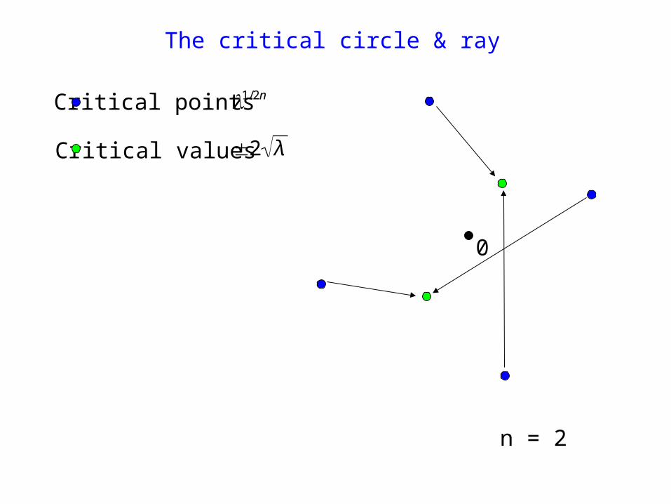
The critical circle & ray

The critical circle & ray
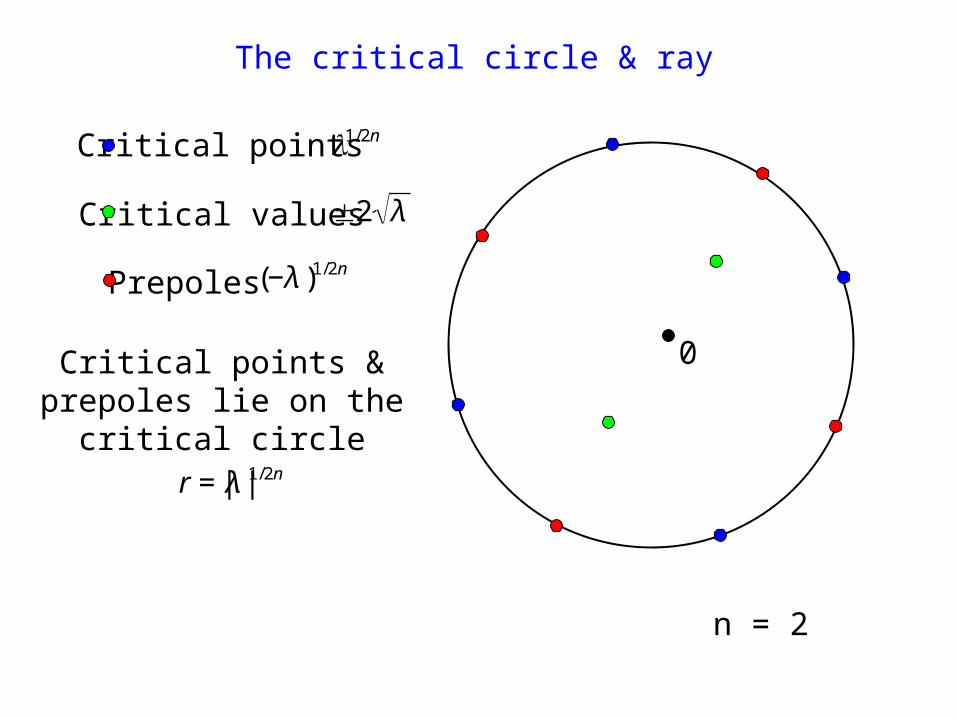
Critical points
€
λ1/2n

The critical circle & ray
Critical points
€
λ1/2n
n = 2
0

The critical circle & ray
Critical points
€
λ1/2n
Critical values
€
±2 λ
n = 2
0
The critical circle & ray
Critical points
€
λ1/2n
Critical values
€
±2 λ
n = 2
0

The critical circle & ray
Critical points
€
λ1/2n
€
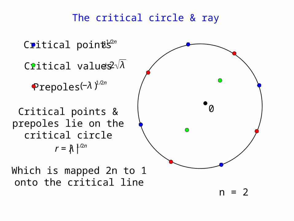
(−λ )1/2nPrepoles
Critical values
€
±2 λ
n = 2
0

The critical circle & ray
Critical points
€
λ1/2n
€
(−λ )1/2nPrepoles
Critical values
€
±2 λ
n = 2
0

The critical circle & ray
Critical points
€
λ1/2n
€
(−λ )1/2nPrepoles
Critical points &prepoles lie on the
critical circle
€
r = |λ |1/2n
Critical values
€
±2 λ
n = 2
0
The critical circle & ray
Critical points
€
λ1/2n
€
(−λ )1/2nPrepoles
Critical values
€
±2 λ
Critical points &prepoles lie on the
critical circle
€
r = |λ |1/2n
n = 2
0
The critical circle & ray
Critical points
€
λ1/2n
€
(−λ )1/2nPrepoles
Critical values
€
±2 λ
Critical points &prepoles lie on the
critical circle
€
r = |λ |1/2n
Which is mapped 2n to 1onto the critical line
n = 2
0

The critical circle & ray
Critical points
€
λ1/2n
€
(−λ )1/2nPrepoles
Which is mapped 2n to 1onto the critical line
Critical values
€
±2 λ
Critical points &prepoles lie on the
critical circle
€
r = |λ |1/2n
n = 2
0

Critical points
€
λ1/2n
Critical values
€
±2 λ
Critical point rays

Critical points
Critical values
€
±2 λ
Critical point raysare mapped 2 to 1 toa ray external to thecritical line, a criticalvalue ray.
€
λ1/2n

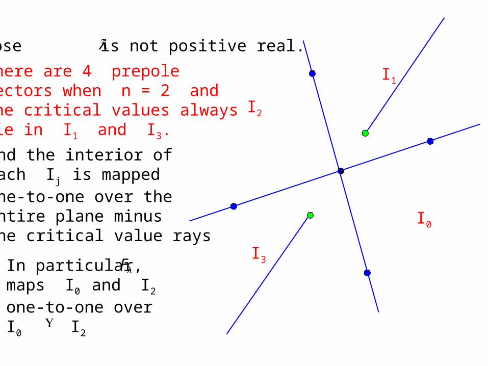
Suppose is not positive real.
€
λ

Suppose is not positive real. Then the critical values do not lie on the critical point rays. €
λ
€
±2 λ
€
−2 λ
€
+ 2 λ
€
λ1/4

I0
I1There are 4 prepole sectors when n = 2 andthe critical values alwayslie in I1 and I3.
I2
I3
Suppose is not positive real.
€
λ

I0
I1
I2
I3
And the interior ofeach Ij is mappedone-to-one over theentire plane minusthe critical value rays
€
λSuppose is not positive real.
There are 4 prepole sectors when n = 2 andthe critical values alwayslie in I1 and I3.
I0
I1
I2
I3In particular,maps I0 and I2
one-to-one overI0 I2 €
Fλ
€
U
€
λSuppose is not positive real.
And the interior ofeach Ij is mappedone-to-one over theentire plane minusthe critical value rays
There are 4 prepole sectors when n = 2 andthe critical values alwayslie in I1 and I3.

Choose a circle in B that is mapped strictly outside itself
€
γ
€
γ
I0
I2

Choose a circle in B that is mapped strictly outside itself
€
γ
€
γ
€
Fλ (γ )
I0
I2

Choose a circle in B that is mapped strictly outside itself
€
γ
€
γ
€
Fλ (γ )
Then there is anothercircle in the trapdoor that is alsomapped to
€
Fλ (γ )
€
υ
€
υ
€
=Fλ (υ )

€
γ
€
υ€
γ
€
υ
Consider the portions ofI0 and I2 that lie between and , say U0 and U2
U2
U0

€
γ
€
γ
€
υ
€
υ
U2
U0
Consider the portions ofI0 and I2 that lie between and , say U0 and U2
U0 and U2 are mappedone-to-one over U0 U2
€
U

€
γ
€
υ
U0
Consider the portions ofI0 and I2 that lie between and , say U0 and U2
U0 and U2 are mappedone-to-one over U0 U2
€
U
So the set of pointswhose orbits lie forall iterations in U0 U2 is an invariant Cantorset
€
U
U2

€
γ
€
υ
Consider the portions ofI0 and I2 that lie between and , say U0 and U2
U0 and U2 are mappedone-to-one over U0 U2
€
U
So the set of pointswhose orbits lie forall iterations in U0 U2 is an invariant Cantorset
€
U

The Cantor set in U0 U2 contains:
€
U
2 points on B
€
∂
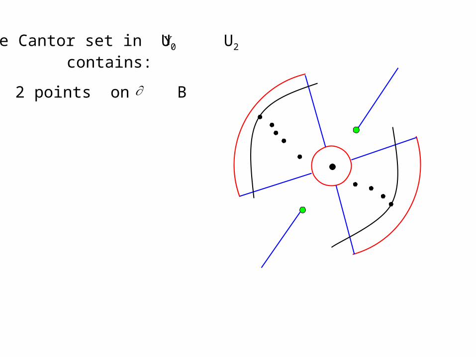
The Cantor set in U0 U2 contains:
€
U
2 points on B
€
∂

The Cantor set in U0 U2 contains:
€
U
2 points on B
€
∂
2 points on T
€
∂

The Cantor set in U0 U2 contains:
€
U
2 points on B
€
∂
2 points on T
€
∂
4 points on the 2 preimages of T
€
∂
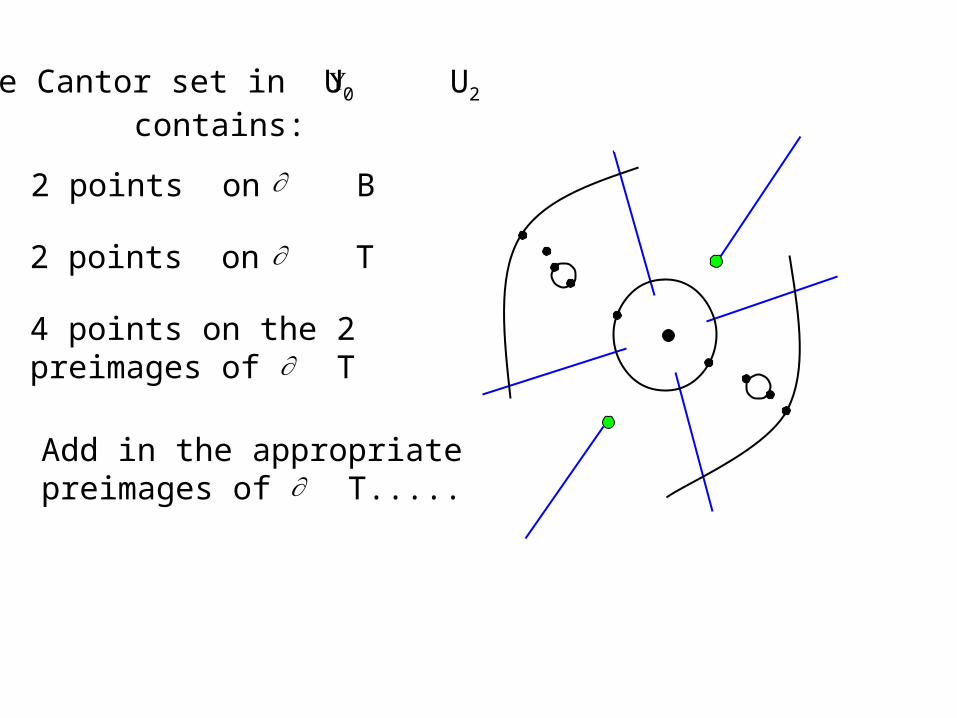
The Cantor set in U0 U2 contains:
€
U
2 points on B
€
∂
2 points on T
€
∂
Add in the appropriatepreimages of T.....
€
∂
4 points on the 2 preimages of T
€
∂

The Cantor set in U0 U2 contains:
€
U
2 points on B
€
∂
2 points on T
€
∂
Add in the appropriatepreimages of Tto get an “invariant”Cantor necklace in thedynamical plane€
∂
4 points on the 2 preimages of T
€
∂

QuickTime™ and aTIFF (LZW) decompressor
are needed to see this picture.
Cantor necklaces in the dynamical plane when n = 2
QuickTime™ and aTIFF (LZW) decompressor
are needed to see this picture.

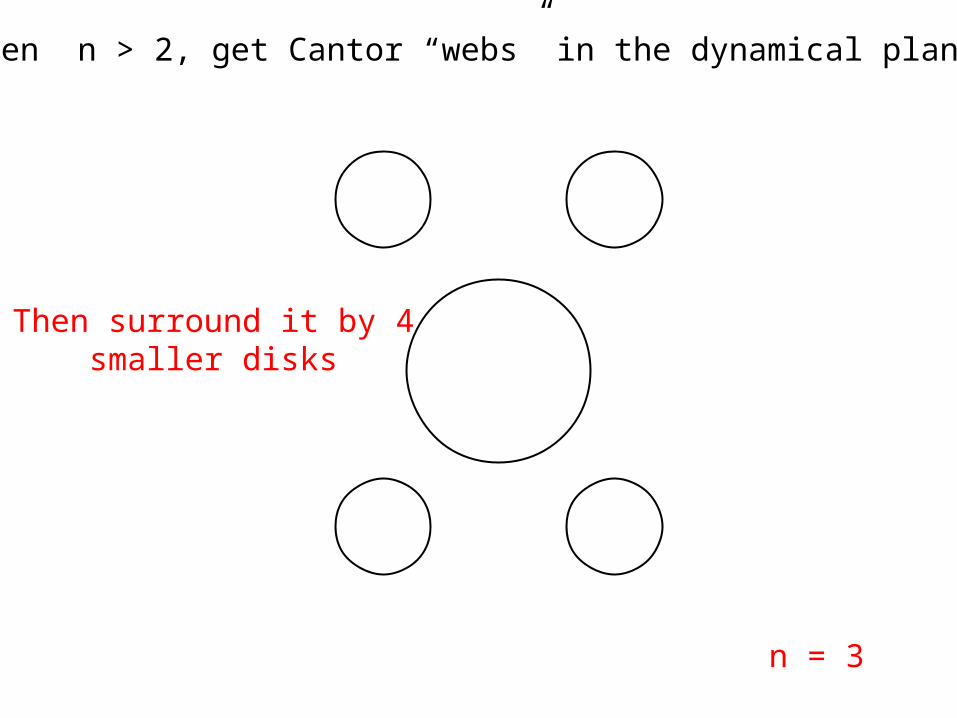
When n > 2, get Cantor “webs” in the dynamical plane:

n = 3
When n > 2, get Cantor “webs” in the dynamical plane:
Start with an open disk....
n = 3
When n > 2, get Cantor “webs” in the dynamical plane:
Then surround it by 4smaller disks
n = 3
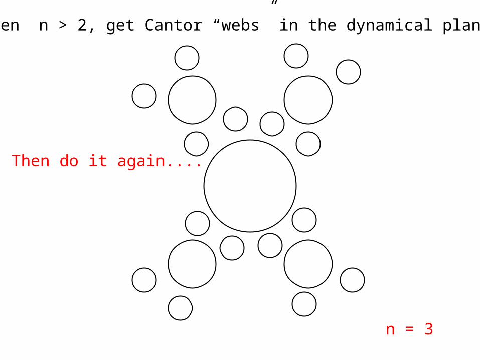
When n > 2, get Cantor “webs” in the dynamical plane:
Then do it again....
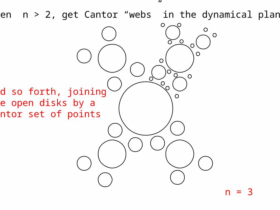
When n > 2, get Cantor “webs” in the dynamical plane:
n = 3
and so forth, joiningthe open disks by a Cantor set of points
QuickTime™ and aTIFF (LZW) decompressor
are needed to see this picture.
QuickTime™ and aTIFF (LZW) decompressor
are needed to see this picture.
n = 4
When n > 2, get Cantor “webs” in the dynamical plane:
n = 3
QuickTime™ and aTIFF (LZW) decompressor
are needed to see this picture.
QuickTime™ and aTIFF (LZW) decompressor
are needed to see this picture.
When n > 2, get Cantor “webs” in the dynamical plane:
n = 3 n = 4
QuickTime™ and aTIFF (LZW) decompressor
are needed to see this picture.
When n > 2, get Cantor “webs” in the dynamical plane:
QuickTime™ and aTIFF (LZW) decompressor
are needed to see this picture.
n = 3 n = 3

QuickTime™ and aTIFF (LZW) decompressor
are needed to see this picture.
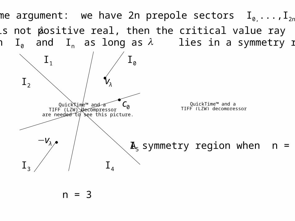
Same argument: we have 2n prepole sectors I0,...,I2n-1
I0I1
I2
I3 I4
I5
n = 3
€
c0

QuickTime™ and aTIFF (LZW) decompressor
are needed to see this picture.
Same argument: we have 2n prepole sectors I0,...,I2n-1
I0I1
I2
I3 I4
I5
If is not positive real, then the critical value ray always lies in I0 and In as long as lies in a symmetry region
€
λ
€
vλ
€
−vλ
n = 3
€
c0
€
λ
QuickTime™ and aTIFF (LZW) decompressor
are needed to see this picture.
QuickTime™ and aTIFF (LZW) decompressor
are needed to see this picture.
Same argument: we have 2n prepole sectors I0,...,I2n-1
I0I1
I2
I3 I4
I5
If is not positive real, then the critical value ray always lies in I0 and In as long as lies in a symmetry region
€
λ
€
vλ
€
−vλ
n = 3
€
c0
€
λ
A symmetry region when n = 3

QuickTime™ and aTIFF (LZW) decompressor
are needed to see this picture.
QuickTime™ and aTIFF (LZW) decompressor
are needed to see this picture.
Same argument: we have 2n prepole sectors I0,...,I2n-1
I0I1
I2
I3 I4
I5
If is not positive real, then the critical value ray always lies in I0 and In as long as lies in a symmetry region
€
λ
€
vλ
€
−vλ
n = 3
€
c0
€
λ
A symmetry region when n = 4

QuickTime™ and aTIFF (LZW) decompressor
are needed to see this picture.
Same argument: we have 2n prepole sectors I0,...,I2n-1
U1
U2
U4
U5€
vλ
€
−vλ
So consider the correspondingregions Uj not including
U0 and Un which contain
€
±vλ
n = 3
€
c0
If is not positive real, then the critical value ray always lies in I0 and In as long as lies in a symmetry region
€
λ
€
λ

QuickTime™ and aTIFF (LZW) decompressor
are needed to see this picture.
n = 3
U1
U2
U4
U5€
vλ
€
−vλ
Each of these Uj are mappedunivalently over all the others,
excluding U0 and Un, sowe get an invariant Cantor set
in these regions.

QuickTime™ and aTIFF (LZW) decompressor
are needed to see this picture.
n = 3
Each of these Uj are mappedunivalently over all the others,
excluding U0 and Un, sowe get an invariant Cantor set
in these regions.
Then join in the preimages of Tin these regions....

QuickTime™ and aTIFF (LZW) decompressor
are needed to see this picture.
n = 3
Each of these Uj are mappedunivalently over all the others,
excluding U0 and Un, sowe get an invariant Cantor set
in these regions.
Then join in the preimages of Tin these regions....
and their preimages....

QuickTime™ and aTIFF (LZW) decompressor
are needed to see this picture.
n = 3
Each of these Uj are mappedunivalently over all the others,
excluding U0 and Un, sowe get an invariant Cantor set
in these regions.
Then join in the preimages of Tin these regions....
and their preimages....
etc., etc. to get the Cantor web

QuickTime™ and aTIFF (LZW) decompressor
are needed to see this picture.
Other Cantor webs
n = 4 n = 5
QuickTime™ and aTIFF (LZW) decompressor
are needed to see this picture.

Other Cantor webs
Next time we’ll see how Cantor webs and necklacesalso appear in the parameter planes for these maps.
QuickTime™ and aTIFF (LZW) decompressor
are needed to see this picture.
QuickTime™ and aTIFF (LZW) decompressor
are needed to see this picture.

Part 4: Internal Rays
QuickTime™ and aTIFF (LZW) decompressor
are needed to see this picture.
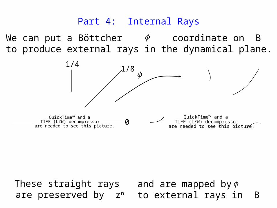
These straight rays are preserved by zn
1/4
0
1/8
We can put a Böttcher coordinate on B to produce external rays in the dynamical plane.
€
ϕ
Part 4: Internal Rays
QuickTime™ and aTIFF (LZW) decompressor
are needed to see this picture.
We can put a Böttcher coordinate on B to produce external rays in the dynamical plane.
QuickTime™ and aTIFF (LZW) decompressor
are needed to see this picture.
1/4
0
1/8€
ϕ
€
ϕ
and are mapped by to external rays in B
€
ϕThese straight rays are preserved by zn

QuickTime™ and aTIFF (LZW) decompressor
are needed to see this picture.
And using the Cantor necklace/web, these can beextended to “internal rays” connecting the
external rays to the origin and passing throughthe Julia set in interesting ways:

QuickTime™ and aTIFF (LZW) decompressor
are needed to see this picture.
And using the Cantor necklace/web, these can beextended to “internal rays” connecting the
external rays to the origin and passing throughthe Julia set in interesting ways:

QuickTime™ and aTIFF (LZW) decompressor
are needed to see this picture.
These two internal rays pass through all the points in the Cantor set of points inthe Cantor necklace as well as through
the appropriate preimages of T:

In the necklace construction, you justpull back appropriate images of theexternal rays in B;

In the necklace construction, you justpull back appropriate images of theexternal rays in B;
0
1/2

In the necklace construction, you justpull back appropriate images of theexternal rays in B;
0
1/2

In the necklace construction, you justpull back appropriate images of theexternal rays in B;
0
1/2

In the necklace construction, you justpull back appropriate images of theexternal rays in B; which then connectup with the appropriate endpoints ofthe Cantor set to produce the internal ray.
0
1/2

Some facts:
QuickTime™ and aTIFF (LZW) decompressor
are needed to see this picture.
When n > 2, there exists an easy-to-constructCantor set of such internal rays, and each crossesinfinitely many others.

Some facts:
QuickTime™ and aTIFF (LZW) decompressor
are needed to see this picture.
And the regions in between these crossingrays give disks on which the map is polynomial-like in the sense of Douady and Hubbard.
€
Fλ is polynomial-like in this disk.
Some facts:
So this enables us to prove the existence ofthe infinitely many baby Mandelbrot setsyou see in the parameter planes:
QuickTime™ and aTIFF (LZW) decompressor
are needed to see this picture.
Some facts:
So this enables us to prove the existence ofthe infinitely many baby Mandelbrot setsyou see in the parameter planes:
QuickTime™ and aTIFF (LZW) decompressor
are needed to see this picture.

Some facts:
So this enables us to prove the existence ofthe infinitely many baby Mandelbrot setsyou see in the parameter planes:
QuickTime™ and aTIFF (LZW) decompressor
are needed to see this picture.

Some facts:
So this enables us to prove the existence ofthe infinitely many baby Mandelbrot setsyou see in the parameter planes:
QuickTime™ and aTIFF (LZW) decompressor
are needed to see this picture.

Some facts:
So this enables us to prove the existence ofthe infinitely many baby Mandelbrot setsyou see in the parameter planes:
QuickTime™ and aTIFF (LZW) decompressor
are needed to see this picture.

Some facts:
And there is a piecewise linear model forthese internal rays that you can embed in the Sierpinski carpet:
QuickTime™ and aTIFF (LZW) decompressor
are needed to see this picture.

Some facts:
And there is a piecewise linear model forthese internal rays that you can embed in the Sierpinski carpet:
QuickTime™ and aTIFF (LZW) decompressor
are needed to see this picture.QuickTime™ and a
TIFF (LZW) decompressorare needed to see this picture.
Some facts:
And finally, this should provide a mechanism (Yoccozpuzzles) to prove what is “obviously” true: that the boundaries of the parameter planes for these maps are simple closed curves (like Milnor’s cubic family).
QuickTime™ and aTIFF (LZW) decompressor
are needed to see this picture.
QuickTime™ and aTIFF (LZW) decompressor
are needed to see this picture.
n = 4 n = 7