Embed Size (px)
Citation preview
DOCUMENT RESUME
ED 043 934 EA 001 681
AUTHORTITLE
INSTITUTICN
REPORT NOPUB DATENOTE
EDRS PRICEDESCRIPTORS
Zabrowski, Edward K.; And OthersStudent-Teacher Population Growth Model. WorkingPaper.National Center for Educational Statistics(DHEW /OE) , Washington, D.C.0E-1005568120p.
EDRS Price MF-$0.50 HC-$6.10*Computer Programs, *Mathematical Models,*Population Growth, *Population Trends, *SchoolStatistics
ABSTRACTThis mathematical model of the eaucational system
calculates information on population groups by sex, race, age, andeducational level. The model can be used to answer questions aboutwhat would happen to the flows of students and teachers through theformal educational system if these flows are changed at variousstages. The report discusses the major assumptions, methodology, andmathematical properties of the model, and the scope of its data. Inaddition to detailed calculations for 140 population groups from 1959to 1970, the impact of selective changes in the model's parameters onthe composition of the educational population is discussed.Appendixes contain tables and charts summarizing various aspects cfthe model, including the Dynamod II computer program. Relateddocuments are EA 001 018; EA 001 062; EA 001 063; EA 001 064; EA 001066; and EA 001 067. (Author /LLR)

V
WORKING PAPER
STUDENT-TEACHER
POPULATION
GROWTH MODEL
U.S. DEPARTMENT OF HEALTH, EDUCATION IL WELFARE
OFFICE OF EDUCATION
THIS DOCUMENT HAS BEEN REPRODUCED EXACTLY AS RECEIVED FROM THE
PERSON OR ORGANIZATION ORIGINATING IT. POINTS OF VIEW OR OPINIONS
STATED DO NOT NECESSARILY REPRESENT OFFICIAL OFFICE OF EDUCATION
POSITION OR POLICY.
I
STUDENT-TEACHER POPULATION GROWTH MODEL
By Edward K. Zabrowskiand
Judith R. ZinterTetsuo Okada
U.S. DEPARTMENT OF HEALTH, EDUCATION, AND WELFARE
Wilbur J. Cohen, Acting SecretaryOFFICE OF EDUCATION: Harold Howe II, Commissioner
0E-10055
ii
A publication of the National Center for Educational Statistics
F. C. Nassetta, Acting Assistant Commissioner
David S. Stoller, Director, Division of Data Analysisand Dissemination
a
a
iii
FOREWORD
The Student-Teacher Population Growth Model (Dynamod II) is amathematical model of the formal American educational system. Itcalculates information on 140 population groups cross-classified by sex,race, age and educational level. It can be used to answer many (butcertainly not all) questions about what would happen to the flows ofstudents and teachers through the formal educational system if theseflows at various stages are changed.
This report touches on several topics. The Introduction discussesthe major assumptions used in developing the model, the scope of the data,and the methodology of the model, including some of the model's mathematicalproperties.
The section "Results and Analysis" first presents the detailed calcu-lations from the model for the 140 population groups, spanning the academicyears from 1959-60 to 1969-70. The discussion "Special Analyses" containssome illustrations of what can be done with a model of this type. That is,the impact on the calculations of the composition of the educationalpopulation caused by making selective changes to the model's parametersare traced through time. Such changes reflect what could be the effectseither of Government policy or of autonomous shifts in tastes, preferencesor habits in the population.
In the Appendixes will be found a large number of tables and chartssummarizing various aspects of the detailed information presented in theResults section. In addition, the Dynamod II computer program is presentedand briefly explained.
The development of a mathematical model quite often rapidly distinguishesthose portions of an existing data base that need to be augmented. Evenwith a relat!..vely abbreviated model such as Dynamod II the gap in theamount of available data compared to that required for the model wasconsiderable. As a result of the model's development we now have a muchclearer picture of what additional statistics need to be included in ourgrowing general information systems, and plans for future surveys ineducational statistics will reflect the knowledge gained thereby.
David S. StollerDirector
Division of Data Analysisand Dissemination
CONTENTS
LAO.
Foreword iii
Highlights of the Report viii
Introduction 1Background 1Basic assumptions 1Scope of data 2
Methodology 4
Results and Analysis 14Student-teacher population by population grouping 14Special analyses 21
Limitations of the data 51
vi
TABLESPage
Table 1 Population Groups Used as Inputs to DYNAMOD II . . . 10
Table 2 Age and Educational Categories, with Abbreviations,Used in DYNAMOD II 15
Table 3 DYNAMOD IIby Age and
Table 4 DYNAMOD IIby Age and
Table 5
Table 6
Figure
DYNAMOD IIby Age and
DYNAMOD IIGroups, byto 1969-70
calculations of White Male Population Groups,Educational Category, 1959-60 to 1969-70 . . . 17
Calculations of White Female Population Groups,Educational Category, 1959-60 to 1969-70 . . . 18
Calculations of Nonwhite Male Population Groups,Educational Category, 1959-60 to 1969-70 . . . 19
Calculations of Nonwhite Female PopulationAge and Educational Category, 1959-60
LIST OF ILLUSTRATIONS
Title
20
1 Flow chart of DYNAMOD II computing procedures 72 Secondary school dropouts by sex and race, 1959-60 to
1968-69 22
3 Series D and Series B birth data used in DYNAMOD II,1959-60 to 1969-70 24
4 Comparison of DYNAMOD II population calculations of 0-4year olds, using different birth estimates, 1960-70 . . . 26
5 Comparison of DYNAMOD II population calculations of 5-14year olds, using different birth estimates, 1960-70 . . . 27
6 Comparison of DYNAMOD II calculations of 15-19 year oldsusing different birth estimates, 1960-70 28
7 Results of a one-percent increase in the elementaryschool student retention rate, 1959-60 to 1969-70 . . 30
8 Results of a one-percent increase in the secondaryschool student retention rate, 1959-60 to 1969-70 . . . 31
9 Results of a one-percent increase in the college studentretention rate, 1959-60 to 1969-70 33
10 Results of a one-percent increase in the elementary schoolteachers' retention rate, 1959-60 to 1969-70 34
11 Results of a one percent increase in the secondary schoolteachers' retention rate, 1959-60 to 1969-70 35
vii
LIST OF ILLUSTRATIONS
Figure Title Page
12 Results of a one-percent increase in the college teachers'retention rate, 1959-60 to 1969-70 36
13 Relative increases in the educational population broughton by a one-percent increase in the DYNAMOD II elementaryschool student retention rate, 1959-60 to 1969-70 . . 38
14 Relative increases in the educational population broughton by a one-percent increase in the DYNAMOD II secondaryschool student retention rate, 1959-60 to 1969-70 39
15 Relative increases in the educational population broughton by a one-percent increase in the DYNAMOD II collegestudent retention rate, 1959-60 to 1969-70 40
16 Comparison of the variations in the student-teacher ratiocaused by selected increases in student or teacherretention rates, by level of schooling, 1959-60 to 1969-70 42
17 Hypothetical illustration of the use of DYNAMOD II forpolicy sequencing applied to elementary school student -teacher ratios 45
18 DYUAMOD II estimates of the flows of elementary schoolteachers, 1968-69 to 1969-70 46
19 DYNAMOD II estimates of the flows of secondary schoolteachers, 1968-69 to 1969-70 48
20 DYNAMOD II estimates of the flows of college teachers,1968-69 to 1969-70 4°
21 Hypothesized effects of setting teacher retention ratesequal to survival rates and eliminating all sources ofentry to teaching except through the college studentsector, compared to the original. DYNAMOD II calcula-tions, 1959-60 to 1969-70 50
APPENDIXES
Page
Appendix A Summary Calculations of DYNAMOD II 54Appendix B Tables of the Effects of Using Different Birth
Estimates 73Appendix C Tables of the Effects of Variations in the Retention
Rates of Students and Teachers 82Appendix D Effects of Variations in the Retention Rates of
Students and Teachers 88Appendix E The DYNAMOD II Computer Program 93Appendix F Methodology of Parameter Estimation in DYNAMOD II:
An Annotated Bibliography 107
viii
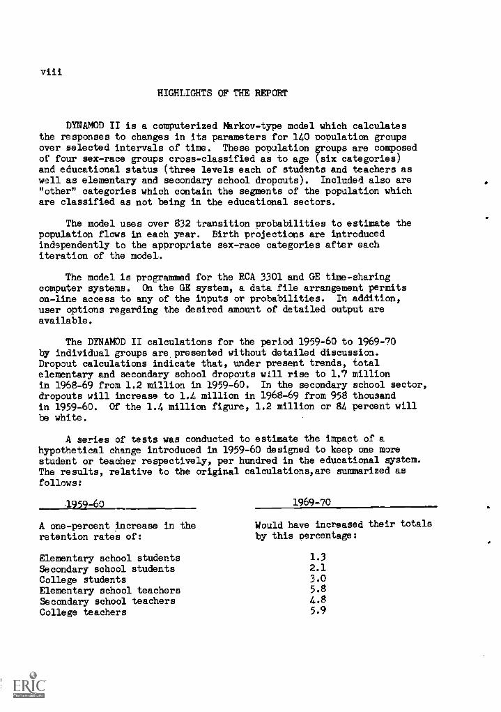
HIGHLIGHTS OF THE REPORT
DYNAMOD II is a computerized Markov-type model which calculatesthe responses to changes in its parameters for 140 Population groupsover selected intervals of time. These population oups are composedgroupsof four sex-race groups cross-classified as to age (six categories)and educational status (three levels each of students and teachers aswell as elementary and secondary school dropouts). Included also are"other" categories which contain the segments of the population whichare classified as not being in the educational sectors.
The model uses over 832 transition probabilities to estimate thepopulation flows in each year. Birth projections are introducedindependently to the appropriate sex-race categories after eachiteration of the model.
The model is programmed for the RCA 3301 and GE time-sharingcomputer systems. On the GE system, a data file arrangement permitson-line access to any of the inputs or probabilities. In addition,user options regarding the desired amount of detailed output areavailable.
The DYNAMOD II calculations for the period 1959-60 to 1969-70by individual groups are, presented without detailed discussion.Dropout calculations indicate that, under present trends, totalelementary and secondary school dropouts will rise to 1.7 millionin 1968-69 from 1.2 million in 1959-60. In the secondary school sector,dropouts will increase to 1.4 million in 1968-69 from 958 thousandin 1959-60. Of the 1.4 million figure, 1.2 million or 84 percent willbe white.
A series of tests was conducted to estimate the impact of ahypothetical change introduced in 1959-60 designed to keep one morestudent or teacher respectively, per hundred in the educational system.The results, relative to the original calculations,are summarized asfollows:
1959-60 1969-70
A one-percent increase in the Would have increased their totalsretention rates of: by this percentage:
Elementary school students 1.3
Secondary school students 2.1
College students 3.0
Elementary school teachers 5.8
Secondary school teachers 4.8
College teachers 5.9

ix
The secondary impacts, or "spillover" of tie retention rate changesalso were traced. That is, the impact on the secondary school studentsector, college student sector, etc., brought )n by increasing theelementary school student retention rate was examined. This was donefor all three student levels. The usual pattern was a dampeningeffect. For example, in the case of increased retention of elementaryschool students, (1.3 percent by 1969-70), the secondary school popu-lation would eventually increase 1.2 percent and the college sectorby less than that, probably .8 percent.1/
Examinations of the effects of student and teacher retentionrate changes on the respective student-teacher ratios showed that forall levels of schooling the ratio was relatively more responsive tochanges in the retention rates of teachers than of students. It isshown that disparities such as these can be employed to advantage bypolicymakers in what is termed "policy sequencing." A description ofpolicy sequencing relating to objectives of decreasing dropout ratessubject to constraints on the permitted level of the student-teacherratio and the allowable action time is presented in the text.
The construction of the model involved the specification andestimation of the population groups' c.ossflows, which provides in-teresting information regarding the structure of the educationalsystem. For example, it is estimated, that of the nearly 1.2 millionelementary school teachers expected to be teaching in 1968-69, 91thousand will leave teaching. New entries from college in 1969-'70,62 thousand, will not be sufficient tc replace the losses, let aloneprovide for a growth increment. Replacement art' provision for growthmainly will have to come from secondary school 1,ransfers (36 thousand)and from outside the system (36 thousand).
The relative importance of entries from outside the system to thethree teaching levels was tested by an extreme case. Within eachteaching sector the retention rates were set to the survival rates(1.0000 minus the death rate), while permitting as sources of entryonly the present flows of college students. The results indicatedthat the elementary and secondary school sectors could meet theirreplacement and growth requirements from within their sectors, ifthe sectors would in fact respond to retention-increasing policies.The college teaching sector, highly dependent on entries from outside
1? The effect had not fully worked itself out by the end of thecalculational interval. Increasing the elementary schoolretention rate by one percent would virtually eliminate elementaryschool dropouts. Knowledgable educators have pointed out thatsome proportion of dropouts probably are uneducable. How manyof these dropouts are "uneducable" is in part a function of howmuch of our resources we would be willing to allocate to theirreclamation. The balance, then, would be the hard core dropout.

the system,could not satisfy the basic requirements from within thesector. Unless marked alterations in the flows of college studentsinto college teaching occur, this dependence on external entriesshould persist.
In the appendixes will be found most of the statistical material
and summary data for the report. Appendix A in particular contains
a presentation of the summary calculations of the model as well asthe projections of the Office of Education and the Bureau of theCensus, against which the calculations were calibrated.

INTRODUCTION
Background
In September, 1966, an unpublished paper entitled "DYNAMO I: AResearch Demographic Model," was completed. That paper demonstratedthe feasibility of applying Markov chain analysis to the growth andcomposition of the educational population of students and teachers.
The model presented in this publication, DYNAMOD II, was developedon the basis of the lessons learned from DYNAMOD I. It is a morefinely structured and consequently more accurate model than wasDYNAMOD I. As such, DYNAMOD II should prove to be of use to alleducational officials, planners and analysts who are interested inexamining the impact of policy alternatives on the educationalpopulation at the national level.
DYNAMOD II's calculations approximate the Population projectionsof other Federal agencies well enough to provide the educationalcomity with "order of magnitude" estimates of the effects ofvariations in certain key items, such as student- and teacher-retention rates or birth rates, until a new model, Student-TeacherAnalysis of Growth, (STAG) becomes operational.
Basic Assumptions
The basic assumptions used in DYNAMOD II are as follows:
1. A Markov -type process is a suitable means for representingthe flows of people among categories. The technical definition ofa Markov process can be found elsewhere. 1/ As the concept pertains toDYNAMOD II, the population is divided into various cross-classifica-tions based on sex, race, age, and the educational categories that thegroups are in. Then estimates, called "transition probabilities" aremade of the chances that a member of a group in one year will stayin that group or move to another specific group the next year. Afterone cycling of the model, the newly formed groups are multiplied bythe appropriate probabilities to determine the structure of thepopulation in the following year. This process can be continuedindefinitely;
1 /William Feller, An Introduction to Probability Theory and ItsApplications, Volume I, Second edition, John Wiley and Sons,Inc.5;;TUrk: 1957)) p. 369. A simpler but less extensivetreatment of Markov chains can be found in John G. Kemeny,J. Laurie Snell and Gerald L. Thompson, Introduction to FiniteMathematics, Second Edition, Prentice-Hall, Inc. (EnglewoodCliffs: 1966), pp. 194-198 and pp. 271-287.
DYNAMOD II is not a true Markov process, at least in the con-
2
2. The transition probabilities are fixed during the calcula-tion interval; and
3. Death rates are fixed during the calculation interval.
The above description can be considered to be a sketch of theway DYNAMOD II operates. Of course, a large computer model whichgrapples with the complexities of reality must be, of itself,complex. Nevertheless, DYNAMOD II provides a capability for analysisnot easily filled by other means. For example, estimates of thenumbers of people in educational policy target populations (such asyoung nonwhite boys in secondary school) are available in DYNAMOD II,but not elsewhere, because that type of data is not collected in suchdetail in most surveys. The 1960 Census of Population collected suchinformation, however, and in conjunction with estimates of transitionprobabilities to describe the flows and crossflows of the population,provided the means for making projections of the numbers in thosegroups for a predetermined number of years.
Furthermore, by hypothesizing the effects that policy changeswould have on the transition probabilities, an assumed impact on thepopulation can be quantified.
Scope of Data
DYNAMOD II is in every sense a large population model. It features
a population divided into:
Footnote 1 continued
ventional sense. One might best consider DYNAMOD II as a Markovprocess superimposed over a growth function representing net births.In a conventional Markov process, one has the alternatives ofeither cycling the basic population (row) vector, P, n timesthrough the transition matrix T, or calculating P(Tn) to determinethe distribution of the various population groups in year n, where(Tn) is the n th power of the matrix T. The occurrence of net birthsin the model prevents the use of the second alternative, even if itwere desired--but the population groups in DYNANDD II must be cycledeach time, to get the needed data on an annual basis.

3
elementary school studentselementary school dropoutssecondary school studentssecondary school dropoutscollege studentselementary school teacherssecondary school teacherscollege teachersother (i.e., persons who are neither students nor active teachers)
The population is further divided by sex and race (i.e., white andnonwhite), and into age levels 0-4, 5-14, 15-19, 20-24, 25-44 and 44 yearsor older. In all, there are 140 separate population groups (includingdropouts and deaths) in DYNAMOD II, which required the estimation of over830 separate probabilities to describe the groups' crossflows amongcategories. A listing of the population groups is given or. pages 10 and 11.
Student and teacher data are centered on the academic year begin-ning in September. Data on the remainder of the population are centeredon April of the following year.
Data for students and teachers include both public and nonpublicschools, but not schools such as residential schools for exceptionalchildren, subcollegiate departments of institutions of higher education,Federal schools for Indians, or schools in Federal installations. Sincethe data from the Bureau of the Census, 1/1,000 sample were forced intoagreement (see "Methodology" below) with those published by the Officeof Education,2/ Office of Education definitions are applicable.
Elementary school students are defined in this paper 'to be thosechildren tn kindergarten through grade 8, and secondary school studentsare those in grades 9 through 12. College student figures apply toopening fall degree-credit enrolled students, full time and part time.The full-time-equivalent concept was not used for students.
The three teacher categories (elementary, secondary and college)are also alined with Office of Education definitions, except that, aswith students, full-time equivalents were not calculated.
It should be noted that gradewise, the elementary- and secondary-teacher categories are not directly comparable to the respective student
.3/ U.S. Department of Health, Education, and Welfare, Office ofEducation, ProJections of Educational Statistics to 1224=71,0E-10030-65 (Washington, D. C.: Supt. of Documents, U.S.Government Printing Office), 1965.

4
categories. That is, a proportion of teachers in grades 7 and 8 areactually classified as secondary for Office of Education definitionalpurposes. The effects of these differences on the student-teacherratios are discussed in Appendix D.
Methodology
The following paragraphs slimmArize the methodology employed inthe development of DYNAMOD II. The methodology of DYNAMOD II involvedtwo distinct problems--the selection of the structure of the mathe-matical model, and the methodology of estimating data inputs. Theseproblems are highlighted .elow.
Mode]. structure. The mathematical form of DYNAMOD II is:
imax
N. = L.a N1Pij + B. where
i
N =
i =
max
j
=
=
Pij
=
a grouping of people;
a sex -race- age - educational level group identifier
for year t;
the highest-level i -type identifier;
a sex-race-age-educational level group identifierfor year t+1;
the probability that an individual in group i willchange to group j (a transition probability); and
= the number of births in year t+1.Bj
In the model, death rates are included as specific P..'s, while births13
are brought in as an exogenous variable.
To illustrate more clearly how a model of this type operates,assume hypothetically that the population is composed of two groups,1 and 2, which represent "young" and "old" respectively. Assumethat:

1
2
B, = 10 per year;
N1= 50 in year t;
N2= 100 in year t; and
the Pij
matrix is
1 2
.7 .3
0 1.0
5
The transition probabilities indicate (row 1) that 70 percent ofthose who are young will stay young, and 30 percent of those who areyoung will become old. In row 2, none of the old can become young.
In year t+1, there will be
50 (.7) + 100 (0.0) + 10 = N1 = 45 young people, and
50 (.3) t 100 (1.0) = N2 = 115 old people (since there isno death rate.)
In like manner, the calculations for year t + 2 will produce
45 (.7) + 115 (0.0) + 10 = N1 = 41.5 young people, and
45 (.3) + 115 (1.0) = N2= 128.5 old people.
With such a large model as DYNAMOD II, the calculating proceduresare slightly more involved than those 4ndicated in with the exampleshove, depending on the type of computer being used.
DYNAMOD II recently has been run on two computing machines--theRCA 3301 and the GE-235 time-sharing system. One of the convenientfeatures of the time-sharing system is that data files can be createdand left in disk storage for use "on stream" or at another time. Thisfeature is exploited for the DYNAMOD model by creating four datafiles: white males, white females, nonwhite males and nonwhite females.Within each file the number of people in each subgroup and theirrespective transition probabilities are stored according to identi-fiable line number addresses.

6
These data files contain the number of people in the variouscategories, birth vector elements, and the transition probabilities.The files are then united with the computer program and thecalculational process proceeds in the manner shown in figure 1.1/
To temporarily change the parameters for analytical output runs,a few simple steps are followed that instruct the time-sharing systemto duplicate the files. Next, the line number address is retyped,the new line of data is entered, and so on, until all changes havebeen introduced. If the number of changes is small, they can be made"on stream." Then the program is rerun using the new data files.After that, the new files can be saved or deleted. The old filescontaining the base data are undisturbed in the process.
Presently, there are 3 variations of the time-sharing computerprogram for DYNAMOD II. One program prints out data for each of the140 population groups as well as selected subtotals for each yaar inthe interval of calculation. Another program permits the user toselect predetermined output combinations by responding to a seriesof preprogrammed questions. The third program merely prints outselected subtotals for the four sex-race groups.
Data inputs. The Bureau of the Census 1/1,000 sample of the 1960Census unit records served as the primary data source for the DYNAMOD IIinputs. Several adjustment procedures were necessary, however, totransform the Census data into a form acceptable as final input, asdescribed in the following paragraphs.
First, the DYNAMOD II design requires that the individual popu-lation groups be mutually exclusive. That is, an individual must beclassified as either a student or a teacher-- he cannot be both. TheBureau of the Census, tape did not meet this requirement, so it wasnecessary to allocate individuals manually to one specific group.This was done using income as a criterion. For example, an individualclassified as both :tudent and teacher would be allocated to thestudent group if his income was less than $3,000. If his income was$3,000 or more he would be classified as a teacher. Although theuse of income as a criterion was known to be a less than perfectdiscriminant, its use did minimize significantly the assignment ofteachers to student categories. This can be readily shown by a table offaculty salaries.A/
1/ A detailed description of the DYNAMOD II computer program ispresented in William K. Winters, DYNAMOD II in a Time-SharingEnvironment, U.S. Office of Education, National Center forEducational Statistics, Technical Note No. 45, October 23, 1967.
4/ U.S. Department of Health, Education, and Welfare, Office ofEducation, Digest of Educational Statistics. 1962, 0E-10024,Bulletin 1963, No. 10, table 68.
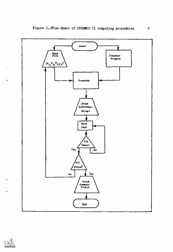
Figure 1.-Flow chart of DYNAMOD II computing procedures 7
ReadFile
1413.1.PiPs)
Start
111
ComputerProgram
Computer
PrintIndividual
Groups
Year
NextYear
AllYears?
All
Piles?
No Yes
Pr irrtSummaryTotals
£nd
8
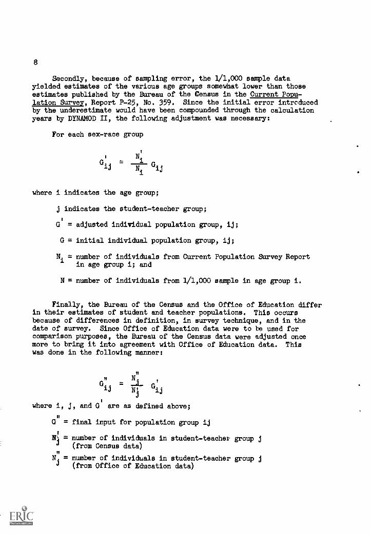
Secondly, because of sampling error, the 1/1,000 sample datayielded estimates of the various age groups somewhat lower than thoseestimates published by the Bureau of the Census in the Current Popu-lation Survey, Report P-25, No. 359. Since the initial error introducedby the underestimate would have been compounded through the calculationyears by DYNAMOD II, the following adjustment was necessary:
For each sex-race group
1
Gi
= Nij
GNi
ij
where i indicates the age group;
j indicates the student-teacher group;
G = adjusted individual population group, ij;
G = initial individual population group, ij;
Ni = number of individuals from Current Population Survey Reportin age group i; and
N = number of individuals from 1/1,000 sample in age group i.
Finally, the Bureau of the Census and the Office of Education differin their estimates of student and teacher populations. This occursbecause of differences in definition, in survey technique, and in thedate of survey. Since Office of Education data were to be used forcomparison purposes, the Bureau of the Census data were adjusted oncemore to bring it into agreement with Office of Education data. Thiswas done in the following manner:
G. =lj N, Gij
where i, j, and G are as defined above;
G = final input for population group ij
113 = number of individuals in student-teacher group j(from Census data)
N4 = number of individuals in student-teacher group j4 (from Office of Education data)
9
When the numbernof students or teachers in these individualpopulationgroups(G..ij )differed from G
ijas a result of the adjust-
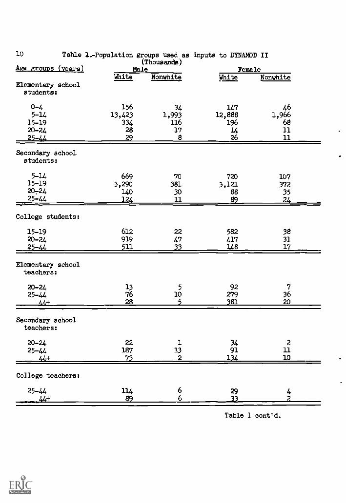
ments just described, the net change was absorbed by the "Other"category. Thus, the input by age was kept in agreement with thoseestimates from the Current Population Survey,Raport No. 359. Thefinal inputs are shown in table 1.
Birth projections in absolute numbers by sex and race were usedin the model, as opposed to the rate concept used for deaths. (SeeDeath rates below.) Two sets of birth data were utilized in DYNA-MOD II. The first was Series B as published by the Bureau of theCensus.V These data provided information on the numbers of birthsby race. Estimates of the within-race male-female distributions, notpublished in that document, were made within the Division of OperationsAnalysis.6/
The second set of birth projections used in DYNAMOD II, Series D,was independently estimated (appendix table B-1).2/ It was felt thatthere was a distinct need for an independent set of estimates, becausethere was a marked discrepancy between the published Series B dataand the births actually being realized in the population. The resultsfor both sets of birth projections are presented later in this report.To maintain an approximate reference comparison, however, the Series Bdata have been used in the DYNAMOD II base line calculations, as wellas in the projections where the student- or teacher-retention rateshave been varied.
Wherever applicable, death rates described in Technical notenumber 11 were modified for DYNAMOD II to make use of differential
5./ U.S. Bureau of the Census, Current Population Reports, PopulationEstimates, Series P-25, No. 345, "Projections of the White andNonwhite Population of the United States, by Age and Sex, to1985," July 29, 1966. These birth projections are slightlylower than those used in the Series E projections which arebased mainly on Current Population Reports, Series P -25, No. 329.
The proportions used to allocate male and females within the raceswere the same as those shown in paper by T. Okada, "Birth and DeathProjections Used in Present Student-Teacher Population Growth Model,"Technical Note Number 11, December 14, 1966.
2/Ibid.
10 Table 1.-Population groups used as inputs to DYNAMOD II(Thousands)
Age groups (years) Male Female
Elementary schoolstudents:
White Nonwhite White Nonwhite
0-4 156 34 147 465-14 13,423 1,993 12,888 1,966
15-19 334 116 196 6820-24 28 17 14 1125-44 29 8 26 11
Secondary schoolstudents:
5-14 669 70 720 10715-19 3,290 381 3,121 37220 -24 140 30 88 3525-44 124 11 89 24
College students:
15-19 612 22 582 3820-24 919 47 417 31
25-44 511 33 148 17
Elementary schoolteachers:
20-24 13 5 92 7
25-44 76 10 279 36
44+ 28 5 381 20
Secondary schoolteachers:
20-24 22 1 34 2
25-44 187 13 91 11
44+ 73 2 134 10
College teachers:
25-44
44+
11489
6
62933
42
Table 1 cont'd.
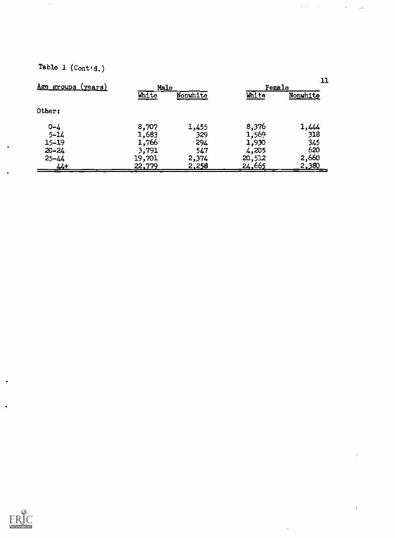
Table 1 (Cont'd.)
Age groups (years) Male Female11
Other:
White Nonwhite White Nonwhite
0-4 8,707 1,455 8,376 1,4445-14 1,683 329 1,569 318
15-19 1,766 294 1,930 34520-24 3,791 547 4,205 62025-44 19,701 2,374 20,512 2,660
22,779 2,258 24,665 2,380
12
mortality rates by occupation.g/ For male teachers, separate mortalityrates were obtained for both white and nonwhite from mortality ratesbased on occupation and age grouping. Their female counterparts werederived by assuming that the female teacher population exhibited thesame male-to-female mortality ratios as in the general population./
Mortality rates for college students in the 15-19 age intervalwere assumed to be the same as for teachers in the 20-24 year interval,which are less than those for the general population of 15-19 year olds.College students in the remaining age intervals were assumed to have thesame death rates as teachers. For elementary and secondary schoolstudents, death rates used in the model were those for the general popu-lation. (See appendix table B-6 for the death rates actually used inDYNAMOD II.)
Estimates of transition probabilities.- The estimating procedurescan be summarized briefly as follows:
1. First approximations to the probabilities for males and femaleswere developed from whatever data sources could be utilized, as well asfrom theoretical and empirical knowledge of the problem.
2. The male and female transition probability matrices were thenadjusted by iterating the population several times, comparing theresults to reference data, adjusting the probabilities, reiterating, etc.,until the fit to the reference data was deemed acceptable.
3. Next, the male and female transition probability estimates were"factored" into their four respective age-race transition matrices.For example, the male elementary school student retention probabilitywas broken into the retention rates for those white and nonwhitestudents who were 0-4, 5-14, 15-19, 20-24, and 24-44 years of age,respectively. The original estimates of the age-education transition
U.S. Department of Health, Education, and Welfare, Public HealthService, National Vital Statistics Division, "Mortality by Occupa-tion and Industry Among Men 20 to 64 Years of Age: United States,1950," Vital Statistics-Special Reports, Vol. 53, No. 2, September,1962. (Washington, D.C.: Supt. of Documents, U.S. GovernmentPrinting Office), table 2.
9-/ U.S. Department of Health, Education, and Welfare, Public HealthService, National Center for Health Statistics, Vital Statisticsof the United States, Vol. II - "Mortality, Part A." (Washington,D.C.: Supt. of Documents, U.S. Government Printing Office, 1966),table 1-25.
13
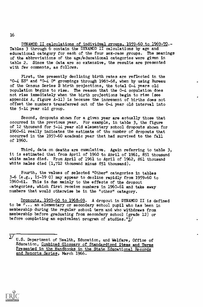
probabilities were completely mechanical. Thus, selected manualadjustments to render these estimates logically acceptable were requiredbefore computerized iterations could take place. As an example,consider the fact that the probability of a 0-4 year old child becoming5-14 years old next year is roughly .2. In initial calculations, .2would be multiplied by the probability of remaining an elementaryschool student. However, the probabilities of age and educationalstatus are not independent, at least at the extreme ends of the agedistributions. In fact, the probability of a child who is now a 0-4year old elementary school student becoming a 5-14 year old elementaryschool student next year is actually quite high, because nearly all0-4 year old elementary school students are 4 years old. This meantthat the original estimate would have to be adjusted to account forthe lack of statistical independence. The remaining probabilitiesin the matrices were screened in this manner and adjusted when necessary.
4. Finally, the four large matrices were used to iterate thepopulation, primarily by computer calculations. After each iteration,the results were checked with reference data. Because of the largenumber of coefficients involved, the initial corrections were made tothe white males matrix, with manual iterations made to that group todetermine whether or not the approximate degree of correction desiredwas being achieved. The next step was to change the coefficients ofthe other three matrices proportionately and recompute the 10-yearcalculations. This process was continued until the calculations allfell within the acce?table tolerance limits.
14
RESULTS AND ANALYSES
Presented below are the results of the computer calculations forDYNAMOD II and some special analyses indicative of the types ofinformation the model can provide.
Student-Teacher PoulationtionGrouing
One of the advantages of DYNAMOD II is that it is directed indetail toward those population groups which are, by and large, thetarget3 of policymakers. As an example, one of the specific groupsin DYNAMOD II is: "male nonwhites 15-19 years of age who are insecondary schools." This group, among many others, has its owneducational flow characteristics and, therefore, is suitable as apolicy target.
One of the disadvantages of working with relatively minute groupsis the scarcity of reference data against which the calculations canbe calibrated. As a result, the relative error of the calculation forindividual groups may be substantially higher than is the case forthe more aggregated groupings, such as "nonwhite males." Since a modelreally is never complete, changes will be made to the parameters asadditional information becomes available, and over a period of time,the accuracy of the detail should improve.
The enormity of space required to show the hypothesized effectsof policy changes on individual groups precludes that type of pre-sentation in this publication. However, the individual groupcalculations for a 10-year periol are presented below for the reader'sinspection ,l/
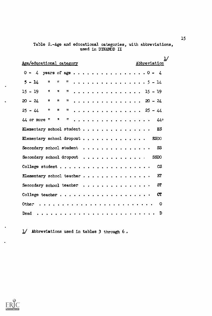
Age and educational category abbreviations. Table 2 contains alisting of the age and educational categories used in DYNAMOD II andthe abbreviations of those categories used in tables 3, 4, 5, and 6.Wien the age and educational categories are combined, there are 35acceptable combinations used for each of the four sex-race groups./
The 1959-60 academic year is not counted as a calculation since itis merely a relisting of the inputs. Thus, 11 years of data arepresented, but only 10 years are considered as calculations in themodel.
Impossible combinations, such as "0-4 year old college students"were screened out. Other possible combinations did not appearon the sample data tape and were not included because of the verysmall numbers of people involved.
15
Table 2. -Age and educational categories, with abbreviations,used in DYNAMOD II
1/Age/educational category Abbreviation
0 4 years of age 0 - 4
5 -14 n n 5 - 14
15 - 19 n n n 15 - 19
20 - 24 n n it 20 - 24
25 - 44 n n n 25 44
44 or more 44+
Elementary school student ES
Elementary school dropout ESDO
Secondary school student SS
Secondary school dropout SSDO
College student CS
Elementary school teacher ET
Secondary school teacher ST
College teacher CT
Other 0
Dead
1/ Abbreviations used in tables 3 through 6.
16
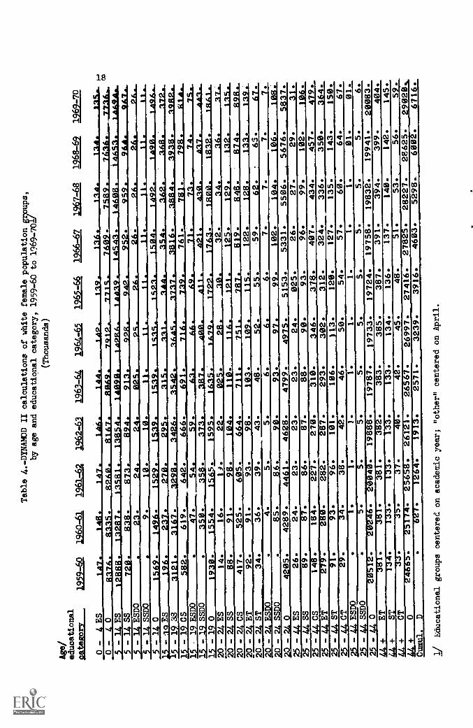
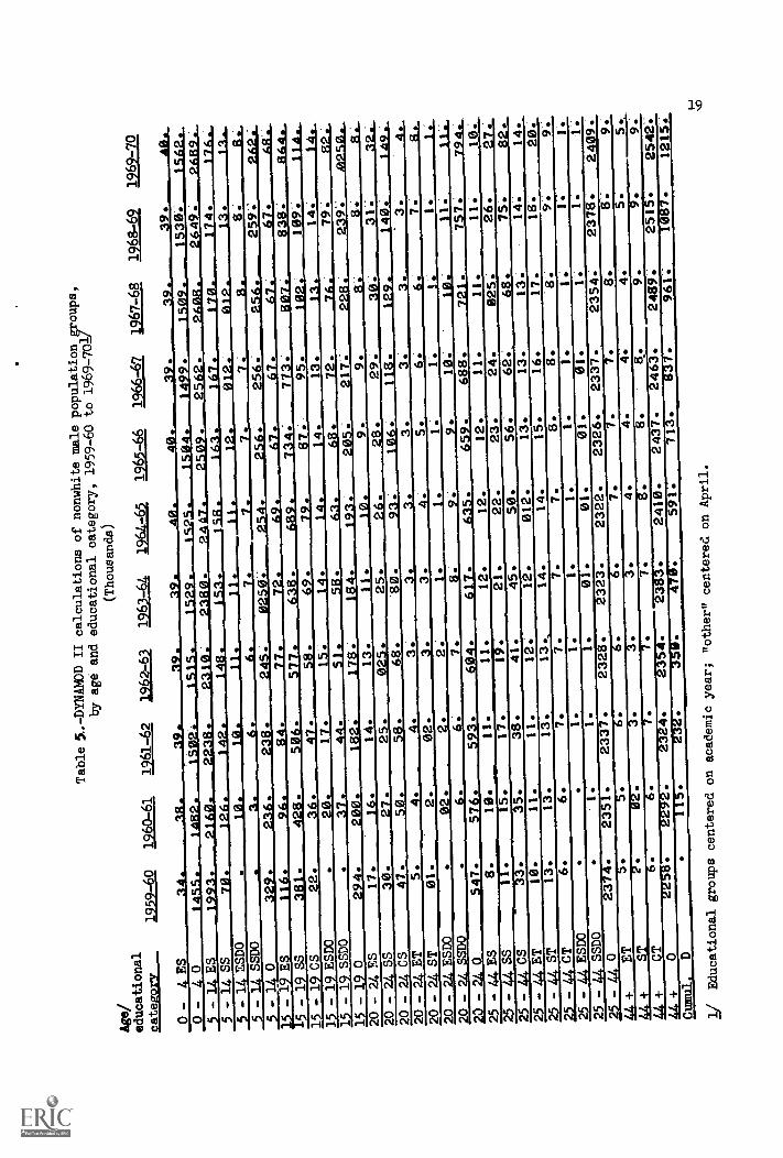
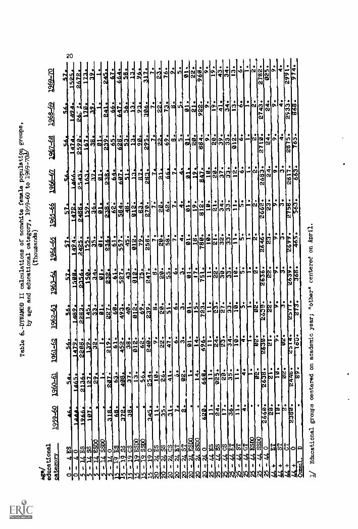
DYNAMOD II calculations of individual aroups, 1959-60 to 1969 -70,-Tables 3 through 6 contain the DYNAMOD II calculations by age andeducational category for each of the four sex-race groups. The meaningsof the abbreviations of the age/educational categories were given intable 2. Since the data are so extensive, the results are presentedwith few comments, as follows.
First, the presently declining birth rates are reflected in the"0-4 ES" and "0-4 0" groupings through 1967-68, when by using Bureauof the Census Series B birth projections, the total 0-4 years oldpopulation begins to rise. The reason that the 0-4 population doesnot rise immediately when the birth projections begin to rise (seeappendix A, figure A-11) is because the increment of births does notoffset the numbers transferred out of the 0-4 year old interval intothe 5-14 year old group.
Second, dropouts shown for a given year are actually those thatoccurred in the previous year. For example, in table 3, the figureof 12 thousand for 5-14 year old elementary school dropouts shown for1960-61 really indicates the estimate of the number of dropouts thatoccurred in the 1959-60 academic year that had survived to the fallof 1960.
Third, data on deaths are cumulative. Again referring to table 3,it is estimated that from April of 1960 to April of 1961, 851 thousandwhite males died. From April of 1961 to April of 1962, 861 thousandwhite males died (1,712 thousand minus 851 thousand).
Fourth, the values of selected "Other" categories in tables3-6 (e.g., 15-19 0) may appear to decline rapidly from 1959-60 to1960-61. This is due mainly to the effects of the dropoutcategories, which first receive numbers in 1960-61 and take awaynumbers that would otherwise be in the "other" category.
Dropouts, 1959-60 to 1968-69. A dropout in DYNAMOD II is definedto be v... an elementary or secondary school pupil who has been inmembership during the regular school term and who withdraws frommembership before graduating from secondary school (grade 12) orbeforecompleting an equivalent program of studies."2/
2/U.S. Department of Health, Education, and Welfare, Office ofEducation, Combined Glossary of Standardized Items and TermsPresented in the Handbooks in the State Educational Recordsand Reports Series, March 1966.
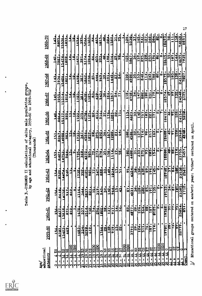
Table 3.-DYNAMOD II calculations of white male population grolips,
by age and educational category, 1959-60 to
1969-701/
(Thousands)
Age/
educational
category
1959-60
1960-61
1961-6Z
1962-63
1963-64
1964-65
1965-66
1966-67
1967-68
1968-69
.969 -70,
0- 4 ES
156.
156.
156.
154.
1 S.
3_.
151,
14)3
.14
5.14
3.14
2.14
3.0- 40
8707
.86
77 .
8610
.5 - 14 ES
1342
3.13
818.
1415
8.14
474.
1475
3.14
988.
1517
7.15
314.
1540
6.15
474.
1553
6.5 - 14 SS
bbl.
S71
.91
7:94
2.96
4.98
3.99
_9.
1012
.&10
21.
1028
.lo
na.
5 - 14 ESDO
012.
012.
.L
3.13
.13
,.L
a;14
.14
.14
.14
.5 - 14 SSDO
7.9.
9.10
.10
.10
.10
.10
.10
.5 - 14 0
1683
.16
78.
1716
.17
32.
1735
.17
33.
1722
.17
03.
1690
.16
87.
1494
.15 - 19 ES
334.
337.
344.
352.
360.
367.
375.
381.
387.
391.
195.
15 - 19 SS
3290
.35
14.
3837
.41
25.
4372
.45
86.
4770
.49
28.
5062
.51
74.
5266
.15 - 19 CS
612.
732.
821.
905.
985.
1059
.11
25.
1185
.12
38...
.128
4,...
.-12
21i..
85.
86.
RA
.15 - 19 ESDO
74.
75.
77.
79.
80.
82.
83.
15 - 19 SSDO
296.
319.
347.
373.
395.
413.
430.
.44
4.45
5.46
5.15 - 19 0
1766
.10
82.
943.
888.
878.
892.
916.
943J
969.
993.
1015
.20 - 24 ES
28.
30.
32.
33.
35.
36.
37.
38.
39.
40.
40.
20 - 24 SS
140.
137.
142.
149.
158.
167.
176.
184.
191.
198.
904.
20 - 24 CS
919.
917.
964.
.10
34.
1114
.12
00.
1285
.13
67.
1445
.15
14.
1582
.20 - 24 ET
13.
14.
15.
17.
19.
21.
22.
24.
27.,
29.
31.
20 - 21 ST
22.
34.
43.
51.
58.
64.
71.'
77.
84.
90.
95.
20 - 24 ESDO
.1.
1.
20 - 24 SSDO
82.
87.
95.
102.
108.
113.
118.
122.
125.
128
0 - 24 0
3791
.40
77.
4231
.43
24.
4408
.45
06.
4623
.47
58.
4908
.50
67.
5230
.25 - 44 ES
29.
29.
30.
30.
31.
32.
33..
34.
35.
36.
37.
25 - 44 SS
124.
126.
128.
130.
.133
137.
.142
.14
7.15
3.15
9.16
5.25 - 44 CS
511.
564.
602.
638.
675.
714.
757.
802.
848.
895.
941.
25 - 44 ET
76.
80.
85.
89.
93.
98.
103.
108.
114.
120.
127.
25 - 44 ST
187.
187.
191.
196.
203.
211.
221.
231.
243.
255.
268.
25 - 44 CT
114.
0125
.13
5.14
5.15
4.16
3.17
1.17
9.18
8.19
6.20
4.25 - 44 ESDO
2.
2.2.
2.2.
2.2.
02.
02.
02.
25 - 44 SSDO
6.7.
7.7.
7.7.
8.8.
8.8.
25 - 44 0
1970
1.19
3613
.19
133.
1894
8.18
800.
1861
313
1861
2.18
574.
1857
5.18
615.
1869
3.+
ET
2031
.34
.37
.40
.43
.46
.49
.52
.55
.58
.44+
ST
4.95
.99
.10
3.10
7.11
1.tr
io.
YS.
101.
108
114.
12-0
-12
6.13
2.13
814
4.15
0.'
44 +
027
79.
2305
4.23305.'
2353
8.23
755.
2396
0.24
154.
2434
0.24
519.
2469
5.14
868.
Cumul.
D51
1712.'
2581
.-34
571"
4340
.52
30.
6125
.70
27.
7935
.88
51.
1/ Educational groups centered on acaeenic year; "other" centered on April.
r
Age/
educational
category
,959 -60
1960-61
0 - 4 ES
1417.
148_.
0-
4 0
8336.
8335.
5 - 14 ES
12888.
13287.
5 - 14 SS
720.
838.
5-
14 ESDO
.23
. 9.5
-14 SSDO
.5
-14 0
1569
.14
96.
15 - 1.9ES
196.
237.
15
- 19 33
3121
.31
67.
15
-19 CS
582.
619.
15
19 ESDO
47.
15 - 19 SSDO
.350.
15 - 19 0
1930.
1554.
20 - 24ES
14.
16.
20 - 24 SS
88.
91.
20- 24 CS
417.
525.
20 - 24 ET
92.
91.
36.
20 - 24 ST
34.
20
-24 ESDO
-..
.4.
20
-24 SSDO
.85
.-
24 0
4205
.42
89.
25 -44 ES
26.
24.
25
-44 SS
89.
87.
25
-44 CS
148.
184.
25
-44 ET
279.
280.
25
-44. ST
91.
93.
25
-44 CT
29.
34.
25
-44 ESDO
125
-44 SSDO
..
25
-44 0
2051
2.20
246.
14+
ET
381.
381.
44
+S
T134.
133.
44 +
CT
JJ.
:..
44 +
02466S.
25174.
CUMUL
D6E7.
Table 4, -DYNAMOD II calculations of white female population groups,
by age and educational category, 1959-60 to 1969-701/
(Thousands)
1961
-62
1262.422
1963-64
1964-65
1965 -66
1966-67,
1967-68
1968-69
1969-70
147
146.
144
1A9
119
116.
114.
11441...---- -115 .
8260.
8167
8019.
7919.
7715.
7609.
7589.
m13854.
14090.
149R6.
144f19.
14543.
14608.
.763,63.2af
14653.
1e49e.
_,13581.
873.
894.
913.
99R.
942.
952.
959.
964.
947.
24.
24.
025.
PS.
PA.
260___
26.
26.
26.
10.
10.
.11.
'II.
11.
11.
11.
11.
11.
1529
.15
39.
1539
.1535.
1593.
1504.
1492.
1490.
1496.
270.
295.
315.
'VII.
244.
354.
362.
368.
372.
3298
.34
26.
3542
.2145.
"4737.
3816
. ___
3884
.39
38.
1982.
642.
_66
6.69
1.716.
739.
761.__
781.
798.
R14.
---54a..----522----63t-----E6a---E9t----7U----73s...-242--..---75o
.__417.
.443
....
1832.
1R61.
X24.
37'
.
358.
373.
387.
ARA.
Ali.
491.
430.
1565.
1595.
1635.
1679.
1799.
1763.
1800.
1/.
22.
025.
28.
30.
32.
34c
98.
104.
110.
111.
121.
125.
129.
605.
664.
711.
751.
787.
819.
848.
93.
98.
103.
109.
115.
122.
128.
39.
43.
48.
52.
55.
59.
62.
5.
5.
6.
6.
6.
7.7.
86.
90.
93.
97.
99.
102.
104.
4461..
4628.
4799.
4975.
5153.
5331.
5506.
23.
23.
23.
24.
025.
26.
27.
86.
87.
88.
90.
93.
96.
99.
227.
270.
310.
346.
378.
407.
434.
282.
287.
293.
302.
312.
324.
336.
96.
101.
106.
113.
120.
127.
135.
38.
42.
46.
50.
54.
57.
60.
1.
1.
1.
1.
1.
1.
1.
5.
5.
.5.
5.
5.
5.
5.
20040.
19888.
19787.
19733.
19724.
19758.
19832.
381.
382.
383.
385.
387.
391.
394.
133.
133.
133.
134.
136.
137.
140.
37.
40.
42.
45.
48.
5f7
53.,
2565
8.26
121.
2656
7.26
997.
2741
6.27
825.
2822
7.1264.
1913
.25
71.
3239
.39
16.
4603
.52
98..
2/ Educational groups centered on academic year; "other" centered on April.
874.
5494,..,
133.
139
65.
67.
7.
7.106.
108.
5676.
5837
.29
.31
.10
2.106.
457.
479.
350.
4...6
4.143.
150.
64.
67.
01.
01.
5.
6.
19941.
20083.
399.
404.
142.
145.
56.
59.
2862
5.29
028.
,60
02.
6716.
Age/
educational
category
1959-60
O - 4 ES
O -
0
5 - 14 ES
5 -14 SSESDO
5- 14 SSDO
5 - 14 0
1- 1 ES
34.
1993.
70.
Table 5.-DYNAMOD II calculations of
nonwhite male population groups,
by age and educational category,
1959-60 to 1969-7017
(Thousands)
1960-61
1961-62
1962-63
1963 -64.
1964-65
12.61.716
1966-67
1967-68
1968-69
1969-70
39.
39..
40.
40.___
39.
39.___
39.
40.
5.
1504..
1499:
1509._
1530.
1S6P.
_a160.
2g38.
2310.
2380.
2447.
.2509.
2562.
2608.
2649.
pAgil,;
126.
142.
148.
153.
1
4.
11.
12.
012.
012.
13.
1f4'.
3.
6.
6.
7.
T.
7.
256.
7.
256.
8.
256._
8.
259.:
8.
262.
236.
238.
245:
0250.
254.
15 - 19 CS
15 - 19 ESDO
15 - 19 SSDO
15 - 19 0
20 - 24 ES
20 - 24 SS
20 - 24 CS
20 - 24 ET
20 -
ST
20 - 24 ESDO
OSD
22.
36.
47.-
20.
17.
37.
44.
294.
200.
182.
17.
16.
14.
30.
27.
25.
47.
50.
58.
5.
4.
4.
01.
2.
02.
02.
2.
.
25 - 44
25 - 44 SS
25 - 44 CS
25 - 44 ET
25 - 44 ST
25 - 44 CT
25 -
ESDO
25 - 44 SSDO
25 - 44 0
+ET
44+
ST
44 +
CT
44 +
0
Cumul.
D
----33.
10.
13. 6.
2374. 5.
58.
15.
51.
178.
13.
a2s.
68.3.
69.
14.
58.
184.
11.
25.
80. 3.
79AL
14.
63.
193.
_10.
26.
93.3.
87..
95.
14.
13.
68.
72.
__205.
217:
9.
9.
28.
29.
106.
118.
3.
3.
50
6.
3.
3.
2.
1.
1.
1.
1.
10.
688.
7.
.
0 .
.
10.
11.
11.
12.
12.
12.
15.
17.
1'.
21.
22.
35.
38.
41.
45.
50.
11.
11.
12.
12.
012.
13.
13.
13..
14.
14.
6.
7.
7.
7.
7.
.1.
1.
1.
1.
1.
1.
1.
01.
01.
01.
01.
2351.
2337.
2328.
2323.
2322.
2326....
2337.
5.
6.
6.
t.
7.
23.
56.
13.
15.8.
102.
13.
76.
228j
30.
129.
3..
109:
14.
79:
239:
31:
140:3.
114.
14.
82.
M250. 8.
32..
149:4.
7. 1.
11.
11.
11.
11.
1
24.
025.
68.
13.
13.
16.
17.
8.1.
1.
1
26.
75:
14:
18.9. 1.
27.4_
82.
14.
20.
1.
2354:
2378.
7.
7.
4.
4.
4.
8.
4.
8.
9: 1.
1.
2409. 9.
6.
6.
7.
7.
7.
8.
8.
8.
9.
2256.
2292.
2324.
2354.
2383.
2410.
2437.
2463.
2489.
115.
2.320
350.
470.
591:
713.
837.
9.
251.
961':
1087.
Sr9.
2542.:
1215:
1/ Educational groups centered on
academic year; "other" centered on April.
Age/
educational
Table 6.-DYNAMOD II calculations of nonwhite female populatio4 groups,
by age and educational category, 1959-60 to
1969-701/
(Thousands)
category
1959-60
1960-61
1961 -6
1962-63,
1963-64
1964-65
0 - 4 ES
AA.-
54.
56. _
56.
S7*
0 L-:4 0
5 - 14 ES
_uaukjAral,a472,
1966.
2136.
2208.
1489.
1500.
2356.
5 -14 sS
1 9.
_2283.
14 .
-14 ESDO
29.
32.
33.
34.
SSDO
1.0 .
10
219.
7.
15 -19 ES
68.
63.
60.
61.
15 - 1
SS
452.
493.
2 43
15 - 19 ESDO
13:
012.
012:
012.
15 - 19 SSDO
56.
62.
69.
75.
15 - 19 0
345
254.
240.
239.
247.
20 - 24 ES
11.
10.
9.
8.
8.
20 - 24 SS
35.
26.
22.
20.
20.
20 - 24 CS
AM
.31.
41.
47.
51.
55.
20 - 24 ET
7.
o.
6.
6.
6.
20 - 24 ST
a.
02.
3.
3.
3:
20 - 24 ESDO
1.
01.
01.
01.
20 - 24 SSDO
14.
14.
15.
17.
0 - 24 0
620.
660.
696.
723.
751:
25 -44 ES
11.
11.
11.
11.
11.
24.
23.
22.
23.
27.
30.
25 - 44
ET
36.
35.
34.
33.
33.
25 - 44 ST
11.
11.
10.-
10.
10.
25 - 44 CT
4.
4.
4.
5.
5:
25 - 44 ESDO
1.1.
1.
7.
25 -
SSDO
02.
102.
02.
25 -
06610.
0±
+ET
44 +
ST
-9.
9.
44+
CT
2.
02
102.
3.
3.
44 +
02360.
a44s.
4'314.
2577
2639
Cumul.
D89.
'10
0.
57.
1494.
2425.
155.
35.
01.
61.
557:
012.
79.
258. 7.
20:
58.7. 4.
01.
18.
780.
10.
et.
32.
33.
11.5.1.
2. 3*
26-9g.
1965 -66
1966-67
1967 -68
1968-69
1969-70,
57.
SA.
56.
56.
57.
1472:
1AAA
1474.
1494.
.1525.
2488.
25?0.
26;",),.
2672.
36.
37,
38.
a9.
39.
62.
64.
65.
66.
67.
012.
13.
13.
13:
13.
839'
87.
90.
93.
261---
270.
283.
295.
306.
317.
7.
7.
7:
7.
7.
20.
21.
22.
22.
23.
62.
66.
69.
73.
76.
7.
7.
8.
8.
9.
4.
4.
5.
5.
5.
01.
01.
01.
01._
21.
01.
22.
19.
19.
20.
812:
847.
884.
922.
960.
10.
10.
9.
9:
9.
21.
20.
20.
19:
19.
34:
37.
39.
41:
_43.
33.
33.
33
34.
34.
11.
12:
012.
13.
13.
5.
6.
6.
6.
6.
1.
1:
1:
1:
1.
22.
2.
2.
2.
2662.
2683.
2710.
2743.
2782.
23.
24.
84.
24.
025.
9.
9.
9._
9.
9.
3.
3.
4.
4.
4.
2758.
2817.
2875.
2933.
2991.
66 .
65.
1/ Educational groups centered on academic year; ',other"
centered on April.
21
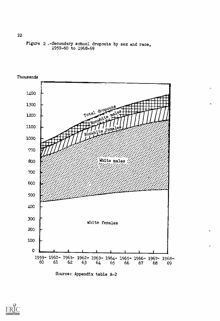
The present estimates of the number of secondary school dropoutsby sex-race group is shown in figure 2. Figure 2 is a band chart.The number of dropouts in a particular group for a given year isindicated in the chart by the vertical distance within a particularband. Whites, who constitute the largest portion of the secondaryschool student population, also constitute the largest numbers ofdropouts.
Under the present set of assumptions, the number of dropoutswill continue to increase in time as the secondary school populationincreases. In the absence of effective policies counteracting thepresent trends, nonwhites will continue to have higher proportionsof the dropout populations than they have of the school population.
1.pecial Analyses
The special analyses presented below illustrate how DYNAMOD IIcan be of use to educational planners, analysts, and decisionmakersin three fields of study: impact analysis, policy sequencing, andstructural studies. These are indicative, but by no means exhaustive,examples of the kinds of information yielded by the model.
Impact analyses explore the effects of changes in the parametersof the model, e.g., birth rates or retention rates. Policy sequenceanalysis is concerned with obtaining feasible solutions to multiple(and sometimes apparently conflicting) policy objectives. Structuralstudies examine the network flows within the system described by themodel and provide perspective on the relative importance of theseflows.
Your topics in impact analysis will be considered. The first,birth variations, gives an indication of how changes in the number ofbirths can affect the educational population over a period of time.The model originally was calibrated using the Bureau of the CensusSeries B birth data. Series D is a set of birth projections developedwithin the Division of Operations Analysis. Only one such variationis presented here, using Series D, but the figures can be varied toany degree desired.
The second, variations in retention rates serves a dual purpose.It shows the approximate changes in the composition of the educa-tional population that might be expected by keeping a higher pro-portion of students or teachers in the system. It also indicatesthe effect of a one-percent error in a retention rate on the esti-mates of the population.
The third, secondary impacts of increasing student retentionrates, traces the effects of changes introduced at one level of thesystem on other parts of the system. For example, anti-dropout
22
Ylgare .-Secortd9.11 sectoolb904 se% aste, race,
1959-60 to 196S-69
1On+.0111
ipso"'41101r.
400
1300
1200
1.100
1000
cf.)0
1100
100
600
500
o
*:0%. **. *
VP f_aa.
e
V II;
tvP'e II,pC4C'
4
a
a
6,4 ei tit*ap
-
4
uhite ..,..::::::::,..-- ....e e ao:::?..%.:::*777l
a
e a
$ f f1.4
11
4e041
II,i41
4
*lb
.7... 0... .:/.. . 7.
.11.e400
300
200
100
01960-1959"
60
a
96162
Source:
Vat" fe"les
9 966'962- 6634 j19664 196656- 6r163
p,ppenax table
S69
23
policies introduced at the secondary school level will affect futurecollege enrollments and the number of teachers produced by theeducational system.
The fourth, student-teacher ratios, probes some of the possibleoutcomes of pursuing such mixed policies as, for example, introducingprograms to keep more students in the system without introducingcompanion programs aimed at increasing teacher retention rates.
Birth variations.- The ultimate validity of any set of populationprojections is known to be highly dependent on the agreement betweenactual and assumed numbers of births. Sudden shifts in the birthrate of the population caused by the outbreak of war, businessconditions, new birth control devices, or from whatever source, canhave marked effects on projections of the numbers of people invarious categories of interest.
It is a great convenience in a population-projections model tohave the flexibility of easily changing the assumed birth rates.A/For example, educational planners and analysts are free to postulateany desirod impact on the birth rate of a policy emanating within oroutside of the educational system, and they can then obtain an esti-mate of the impact on the educational population as a result of thepostulated policy.
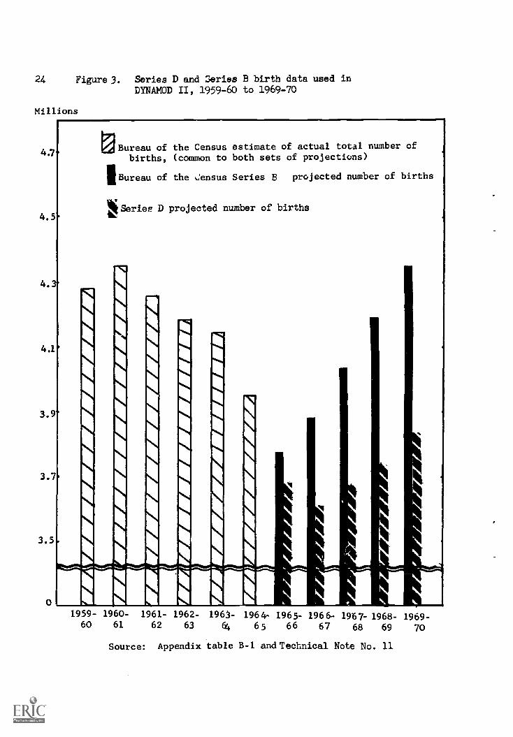
Presented below is an example of the population effects causedby using different assumptions regarding births. Note in figure 3that the birth data for the years 1959-60 through 1964 are commonto both sets of calculations. For those years, estimated actualbirth data were available, and therefore were used. For the remainingyears in the calculation interval, estimates from Series B or Series Dwere used.
As may be expected, differences arise in the calculated (1966-70)population figures according to the particular type of birth figuresused as inputs. Projections of population groups based on the higherSeries B birth projections show up consistently higher than the cal-culations resulting from DYNAMOD II birth estimates. In certain agegroups, differences in the projected population group totals becomemore pronounced with the increased number of years in the calculationinterval.
A/ The same may be said for death rates.
24 Figure 3. Series D and aeries B birth data used inDYNAMOD II, 1959-60 to 1969-70
Millions
4.7
4.5
UBureau of the Census estimate of actual total number ofbirths, (common to both sets of projections)
IIBureau of the ..;ensus Series B projected number of births
Series D projected number of birthsth.
4.3f
4.1
3.9
3.7
3.5
01959- 1960- 1961- 1962- 1961- 1964- 1965- 1966- 1967- 1968- 1969-60 61 62 63 64. 65 66 67 68 69 70
Source: Appendix table B-1 and Technical Note No. 11
25
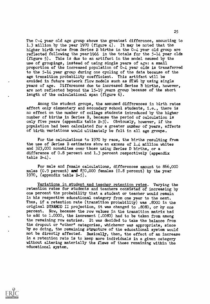
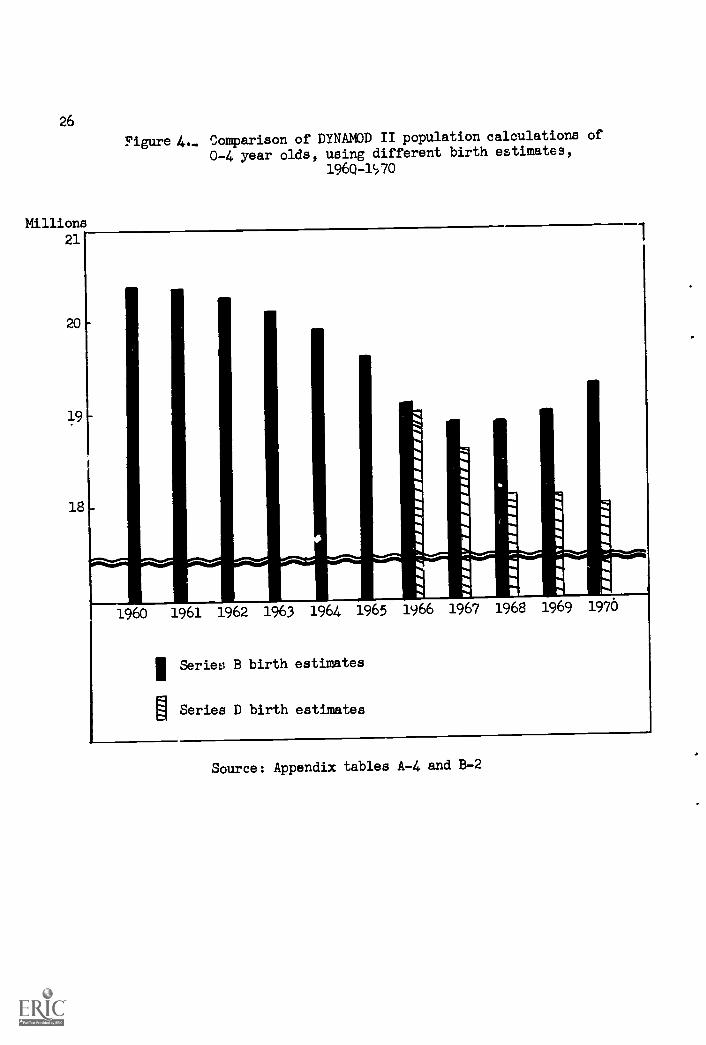
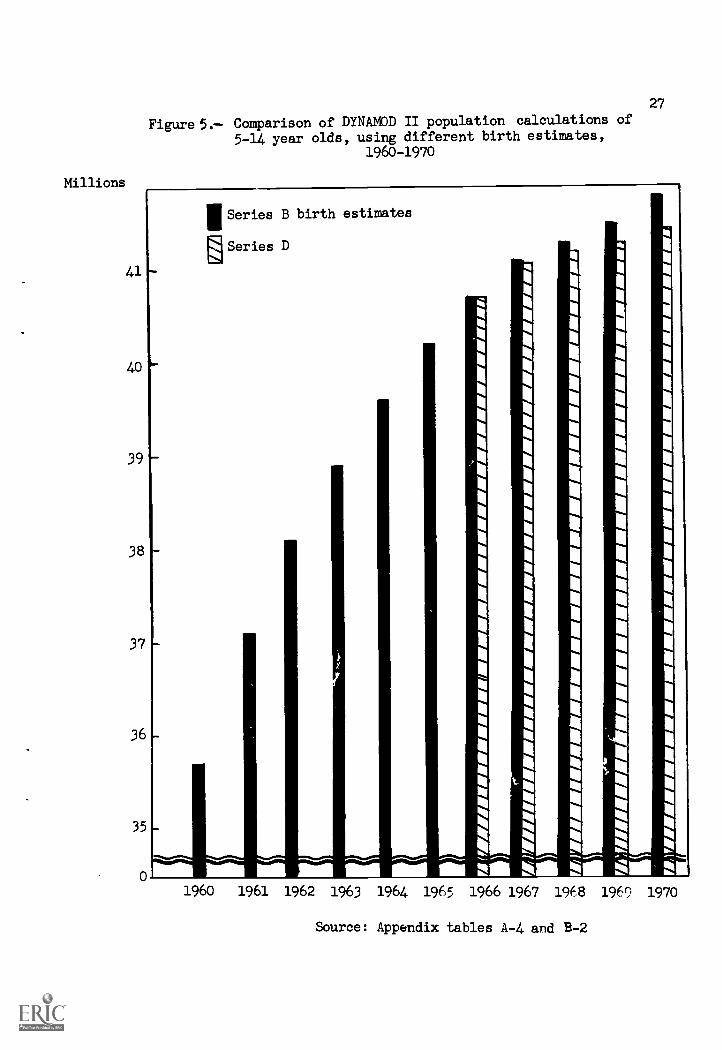
The 0-4 year old age group shows the greatest difference, amounting to1.3 million by the year 1970 (figure 4). It may be noted that thehigher birth rates from Series B births in the 0-4 year old group arereflected following the year 1966 in the totals for the 5-14 year olds(figure 5). This is due to an artifact in the model caused by theuse of groupings, instead of using single years of age: a smallproportion of the increased population of 0-4 year olds is transferredto the 5-14 year group during one cycling of the data because of theage transition probability coefficient. This artifact will beavoided in future network flow models such as STAG by using singleyears of age. Differences due to increased Series B births, however,are not reflected beyond the 15-19 years group because of the shortlength of the calculational span (figure 6).
Among the student groups, the assumed differences in birth ratesaffect only elementary and secondary school students, i.e., there isno effect on the number of college students introduced by the highernumber of births in Series B, because the period of calculation isonly five years (appendix table B-3). Obviously, however, if thepopulation had been calculated for a greater number of years, effectsof birth variations would ultimately be felt in all age groups.
For the calculations to 1970 by race, the births resulting fromthe use of Series B estimates show an excess of 1.4 million whitesand 323,000 nonwhites over those using Series D births, or adifference of 0.8 percent and 1.3 percent respectively (appendixtable B-4).
For male and female calculations, differences amount to 866,000males (0.9 percent) and 8?0,000 females (0.8 percent) by the year1970, (appendix table B-5).
Variations in student and teacher retention rates. Varying theretention rates for students and teachers consisted of increasing byone percent the probability that a student or teacher would remainin his respective educational category from one year to the next.Thus, if a retention rate (transition probability) was .8000 in theoriginal DYNAMOD II projection, it was changed to .8080, or by onepercent. Nowt because the row values in the transition matrix hadto add to 1.0000, the increment (.0080) had to be taken from amongthe remaining row entries. It was decided to take the balance fromthe dropout or "other" categories, whichever was appropriate, sinceby so doing, the remaining structure of the educational system wouldnot be directly affected. BasicalZy, then, the effect of an increasein a retention rate is to keep more individuals in a given categorywithout altering materially the flows of those remaining within theeducational system.
26
Millions21
20
19
18
Figure 4.. Comparison of DYNAMOD II population calculations of
0-4 year olds, using different birth estimates,
196Q-1;70
1960 1961 1962 1963 1964 1965 1966 1967 1968 1969 1976
IISeriei B birth estimates
11 Series D birth estimates
Source: Appendix tables A-4 and B-2
Millions
27
Figure 5.- Comparison of DYNAMOD II population calculations of
5-14 year olds, using different birth estimates,1960-1970
41
40
39
38
37
36
35
Series B birth estimates
ElSeries D
1960 1961 1962 1963 1964 1965 1966 1967 1968 1969 1970
Source: Appendix tables A-4 and B-2
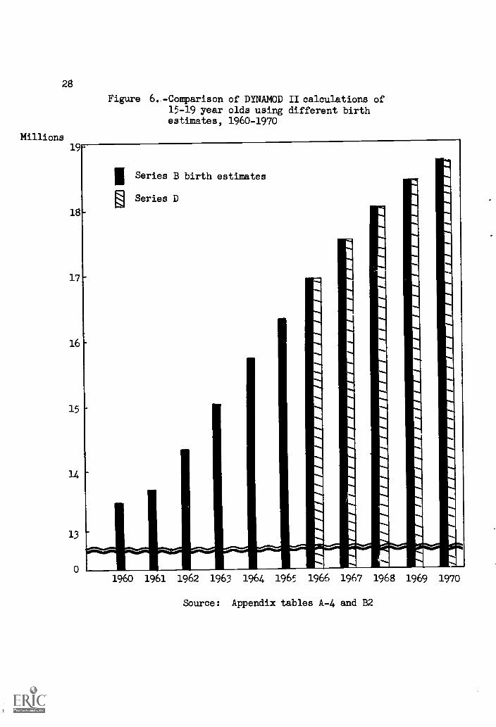
28
Millions
Figure 6..-Comparison of DYNAMOD II calculations of15-19 year olds using different birthestimates, 1960-1970
1960 1961 1962 1963 1964 1965 1966 1967 1968 1969 1970
Source: Appendix tables A-4 and B2
29
The increases in the rates were made one at a time, to avoidconfounding the effects of the changes.
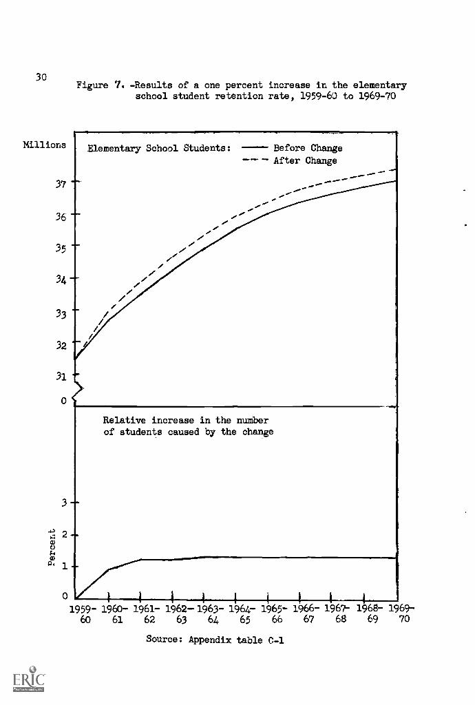
The effect of increasing the elementary school student retentionrate by one percent was to raise the level of the calculation for the1969-70 school year from about 37.0 million to slightly over 37.5million, or by 1.3 percent (figure 7). The relative impact of in-creasing the elementary school student retention rate, that is, thepercent increase in students over the base line projection, waslowest for elementary school students, remaining near one percent overthe entire projection interval. Furthermore, the "time to maximumresponse," i.e., the time required to reach the maximum relativedifference over the base line projection was shortest for this group,reaching the maximum level (1.3 percent) within 4 years.
Knowledge of the relative impact of changes in the educationalpopulation can be of great aid to educational planners, analysts anddecisionmakers by providing them with information regarding requiredchanges in the capacity of the system resulting from the implementationof policies that change the numbers of students or teachers in the system.For example, if planners estimate their capacity requirements on thebasis of a given set of flow rates for students and teachers, they willbe interested in learning what additional changes in capacity may berequired by policies that affect the retention rates of students. Inthe case of elementary school students, for example, an increase of onepercent in the retention rate would require capacity in the systemsufficient to handle the original projections plus about 1.2 to 1.3percent more each year in the interval.
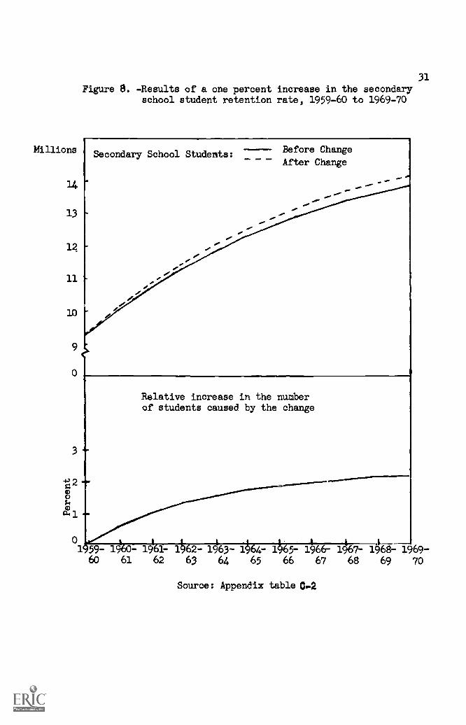
However, for secondary school students, the requirements are some -whet higher. A 1- percent increase in their retention rate wouldraise the DYNAMOD II calculation for 1969-70 from about 13.8 million toover 14.1 million students, or 2.1 percent (figure 8). That is, foreach 1.0-percent increase in the retention rate, an enrollment increaseequal to original projection plus an additional 2.1 percent could beexpected within 10 years.51 Not all the relative impact would be
5/ There are obvious limits to such a statement. First, if the requiredcapacity were not available, then there simply would not be room forthat many students. Second, the changes discussed here are marginal(small) changes, and may not be applicable over large ranges ofpossibilities. For example, a change of 10 percent in the retentionrate may not require places for an additional 21 percent enrollmentin 10 years.
30
Millions
37
36
35
34
33
32
31
0
2
0a)
P.' 1
Figure 7. -Results of a one percent increase in the elementaryschool student retention rate, 1959-60 to 1969-70
Elementary School Students: Before Change
---- After Change
Relative increase in the numberof students caused by the change
0 114 41i1-111959- 1960- 1961- 1962-1963- 1964- 1965- 1966- 1967- 1968- 1969-
60 61 62 63 64 65 66 67 68 69 70
Source: Appendix table C-1
Millions
14
13
12
11
10
-02
31
Figure 8. -Results of a one percent increase in the secondaryschool student retention rate, 1959-60 to 1969-70
Secondary School Students:
de
Before Change
After Change
/Sr
Relative increase in the numberof students caused by the change
0 it I t1 59- 1960- 1961- 1962- 1963- 1964- 1965- 1966- 1967- 1968- 1969-
60 61 62 63 64 65 66 67 68 69 70
Source: Appendix table 0-2
32
expected immediately, as the graph of the relative increases indicates.By the 1964-65 school year, for example, the increased requirements areabout 1.7 percent higher than for the original projections.
As might be expected, there are limits to the relative impacts ofpolicy changes. From the structure of DYNAMOD II, it appears that themaximum relative impact on the number of secondary school students isabout 2.4 percent, reached in about 12 years from the implementationpoint./
The greatest relative impact of all three student categories isachieved with college students (figure 9), where the figure becomes3.0 percent by 1969-70, with an apparent maximum of 3.3 percent inabout 15 years. While this group has the largest relative response toretention policies, the absolute effect by the end of the 10-yearprojection interval is smallest, being only 194 thousand students abovethe original 1969-70 DYNAMOD II projection of 6.6 million students.
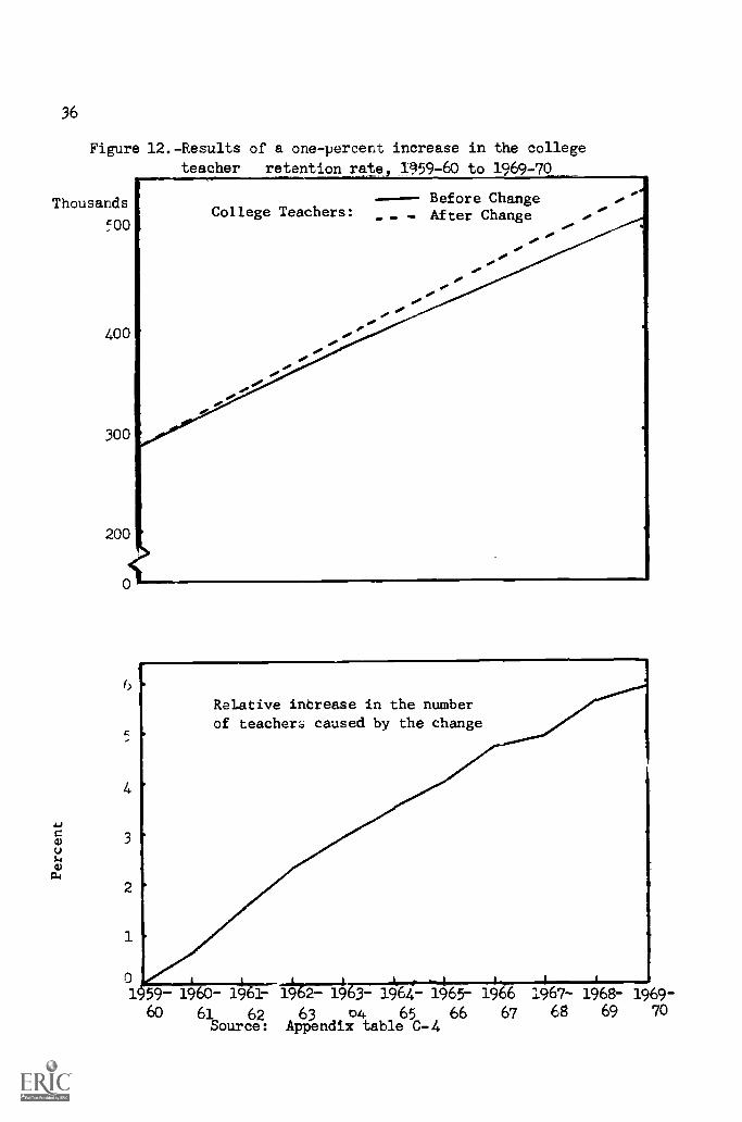
The teaching sector appears to be much more sensitive to increasesin the retention rates than is the student sector, although, of course,the absolute numbers of persons involved are much smaller than is thecase for students. The effects of increasing the retention rates forteachers are shown in figures 10, 11 and 12. The relative responsefactors are quite high by the end of the 10-year interval, being 4.8percent for secondary school teachers, and close to 6 percent forelems-Aary school and college teachers, respectively.
Effective policies aimed at increasing the holding power forteachers in the system, then, would appear to be particularly desirablemeans of increasing the total population of teachers. This seems tobe especially true for college teachers, where a heavy dependence onreturns from the "other" category is required to maintain an acceptablenumber in the system.
Those who are engaged in impact analysis might well ask aboutthe ability of the system to handle changes much larger than one percent.DYNAMOD II cannot answer this question directly. The capacity of thesystems to handle changes in the numbers of people flowing through itmust presently be handled outside of the model. This is not withoutits advantages, however. The ability to calculate the ramificationsof policy changes independently of considerations of the system'scapacity provides a measure of what the economist calls an "opportunitycost." That is, for example, if an otherwise acceptable policy change
The 12-year figure is an estimate taken from the chart, and is notthe result of a statistical fit of the data.
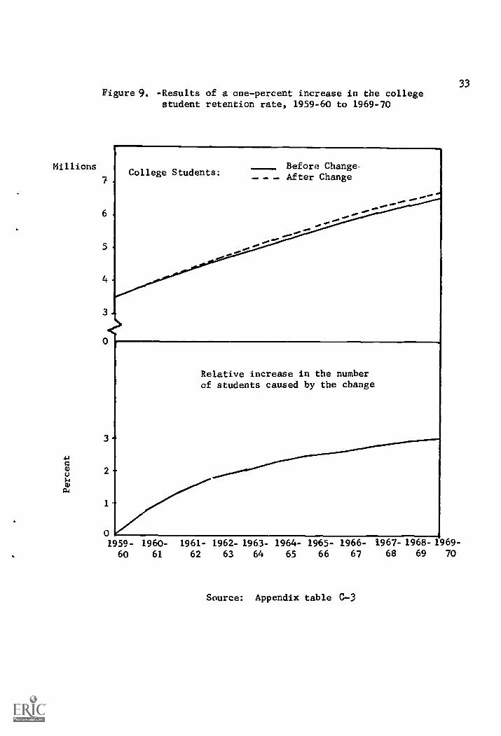
Figure 9. -Results of a one-percent increase in the collegestudent retention rate, 1959-60 to 1969-70
Millions
7
3
2
1
College Students:Before Change.
- - After Change
ao.
Relative increase in the numberof students caused by the change
33
01959- 1960- 1961- 1962- 1963- 1964- 1965- 1966- 1967- 1968- 1969-
. 60 61 62 63 64 65 66 67 68 69 70
Source: Appendix table C-3
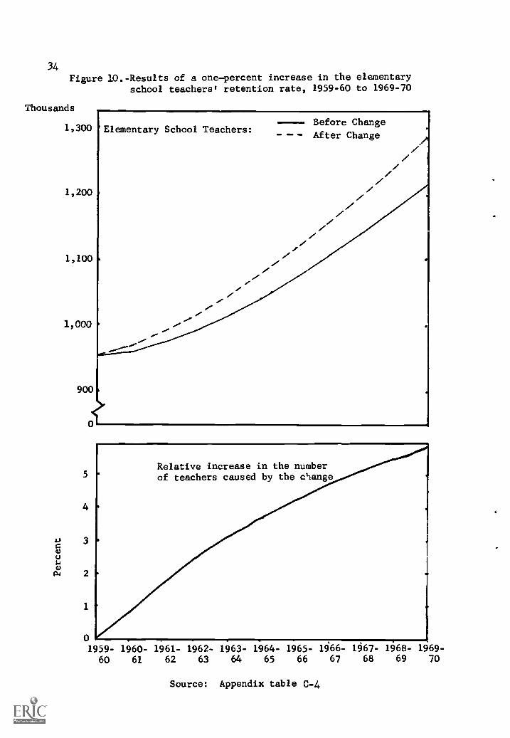
34Figure 10.-Results of a one-percent increase in the elementary
school teachers' retention rate, 1959-60 to 1969-70
Thousands
1,300
1,200
1,100
1,000
900
5
4
1.) 3
2
1
01959- 1960- 1961- 1962- 1963- 1964- 1965- 1466- 1667- 1968- 1969-
60 61 62 63 64 65 66 67 68 69 70
Elementary School Teachers:Before Change
- After Change
Relative increase in the numberof teachers caused by the change
Source: Appendix table C-4
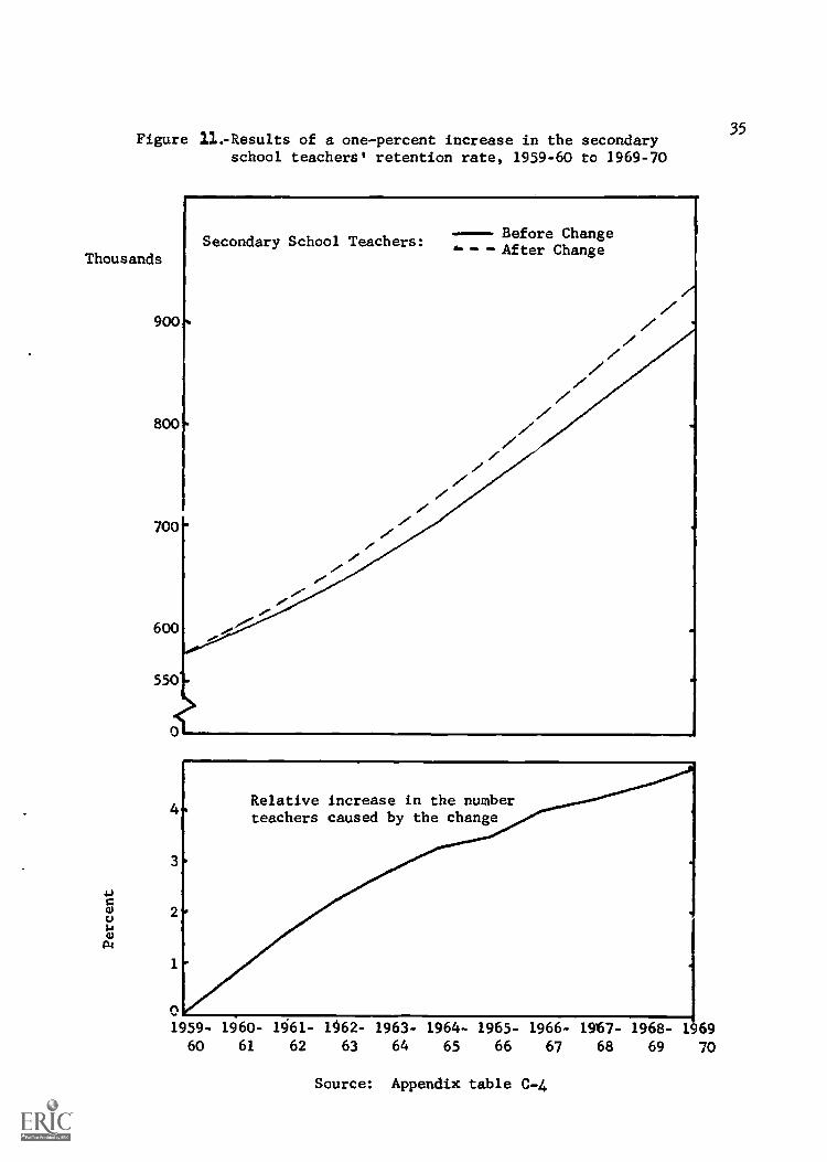
Figure 21.-Results of a one-percent increase in the secondaryschool teachers* retention rate, 1959-60 to 1969-70
Thousands
a)o(i)al
900"
800
700%*
600
550
Secondary School Teachers:
re-
Before Change- - After Change
Relative increase in the numberteachers caused by the change
35
1959- 1960- 1961- 1062- 1963- 1964- 1965- 1966- 19'67- 1968- 196960 61 62 63 64 65 66 67 68 69 70
Source: Appendix table C-4
36
Figure 12.-Results of a one-percent increase in the college
teacher retention rate 1959-60 to 1969-70
Thousands
500
400
300
200
0
College Teachers:
.04
Before ChangeAfter Change
.4*
1
Rotative increase in the number
of teachers caused by the change
59-
60
1960- 19 1-
61 62Source:
19767-It 3- 1964- 1965-
63 04 65 66Appendix table C-4
1966
67
1967-
68
1968-69
1969-70
37
would produce more college graduates than the system could handle, thenan opportunity cost is incurred in terms of foregone college graduatesamounting to the economic value of the difference in the number ofgraduates that could be obtained and those actually expected.
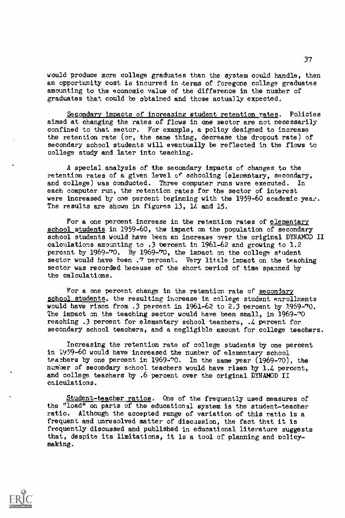
Secondary impacts of increasing student retention rates. Policiesaimed at changing the rates of flows in one sector are not necessarilyconfined to that sector. For example, a policy designed to increasethe retention rate (or, the same thing, decrease the dropout rate) ofsecondary school students will eventually be reflected in the flows tocollege study and later into teaching.
A special analysis of the secondary impacts of changes to theretention rates of a given level or schooling (elementary, secondary,and college) was conducted. Three computer runs were executed. Ineach computer run, the retention rates for the sector of interestwere increased by one percent teginning with the 1959-60 academic year.The results are shown in figures 13, 14 and 15.
For a one percent increase in the retention rates of elementaryschool students in 1959-60, the impact on the population of secondaryschool students would have been an increase over the original DYNAMOD IIcalculations amounting to .3 Percent in 1961-62 and growing to 1.2percent by 1969-70. By 1969-70, the impact on the college studentsector would have been .7 percent. Very little impact on the teachingsector was recorded because of the short period of time spanned bythe calculations.
For a one percent change in the retention rate of secondaryschool students, the resulting increase in college student enrollmentswould have risen from .3 percent in 1961-62 to 2.3 percent by 1969-70.The impact on the teaching sector would have been small, in 1969-70reaching .3 percent for elementary school teachers, .4 percent forsecondary school teachers, and a negligible amount for college teachers.
Increasing the retention rate of college students by one percentin L959-60 would have increased the number of elementary schoolteachers by one percent in 1969-70. In the same year (1969-70), thenumber of secondary school teachers would have risen by 1.4 percent,and college teachers by .6 percent over the original DYNAMOD IIcalculations.
Student-teacher ratios. One of the frequently used measures ofthe "load" on parts of the educational system is the student-teacherratio. Although the accepted range of variation of this ratio is afrequent and unresolved matter of discussion, the fact that it isfrequently discussed and published in educational literature suggeststhat, despite its limitations, it is a tool of planning and policy-making.
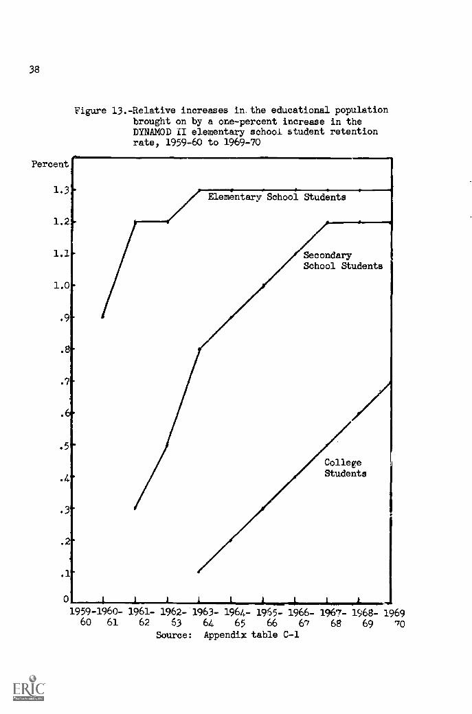
38
Percent
1.3
1.2
1.1
1.0
0
Figure 13.-Relative increases in. the educational populationbrought on by a one-percent increase in theDYNAMOD II elementary school student retentionrate, 1959-60 to 1969-70
Elementary School Students
SecondarySchool Students
CollegeStudents
1959-1960- 1961- 1962- 1963- 1964- 1965- 1966- 1967- 1968- 196960 61 62 63 64 65 66 67 68 69 70
Source: Appendix table C-1
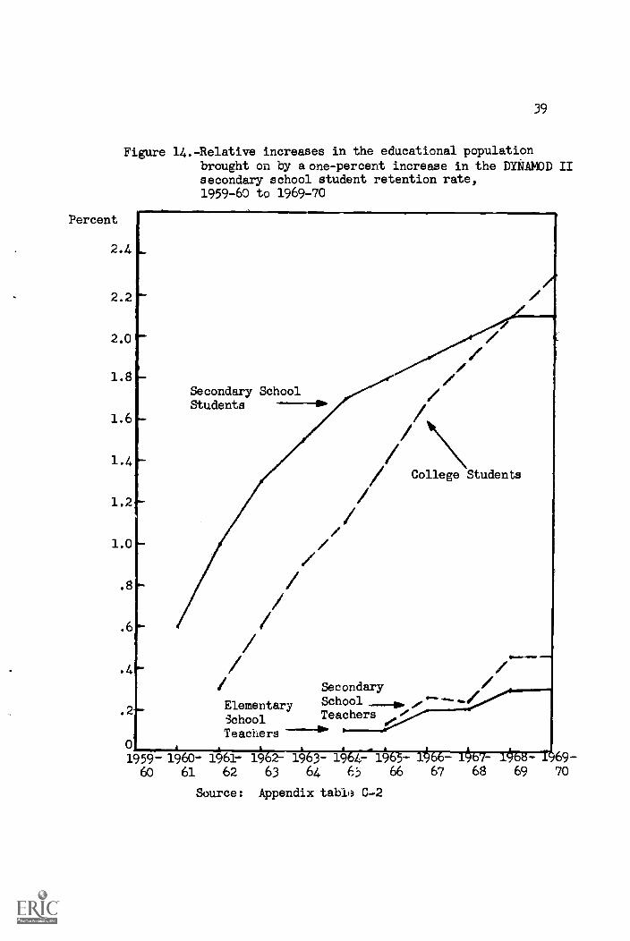
39
Figure 14.-Relative increases in the educational populationbrought on by a one-percent increase in the DYNAMOD IIsecondary school student retention rate,1959-60 to 1969-70
Percent
2.4
2.2
2.0
1.8
1.6
1.4
1.2e-
1.0L
. 2r-
01959- 1960- 19.1- 19o2- 19.3- 19.4- 19.5- 69-
60 61 62 63 64 65 66
Source: Appendix table: C-2
Secondary SchoolStudents
/
It
/// College Students
/ Secondary
Elementary School _11,, ,e"---
School Teachersse
Teachers --11" '
67 68 69 70
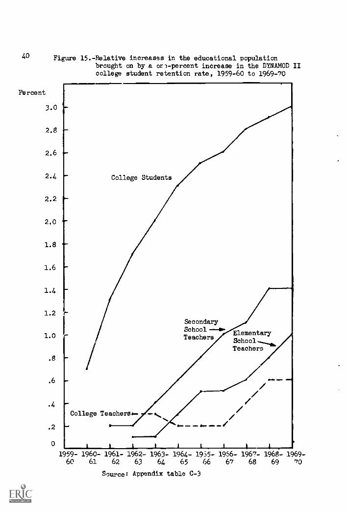
40
Percent
Figure 15.-Relative increases in the educational populationbrought on by a orl-percent increase in the DYNAMOD IIcollege student retention rate, 1959-60 to 1969-70
3.0
2.8
2.6
2.4
2.2
2.0
1.8
1.6
1.4
NNW
/M.
1.2 r
1.0
.8
.6
.4
.2
College Students
College Teachers,
SecondarySchoolTeachers
ElementarySchoolTeachers
0i i 1 I 1 I I I l .
1959- 1960- 1961- 1962- 1963- 1964- 1955- 1966- 1967- 1968- 1969-60 61 62 63 64 65 66 67 68 69 70
Source: Appendix table C-3
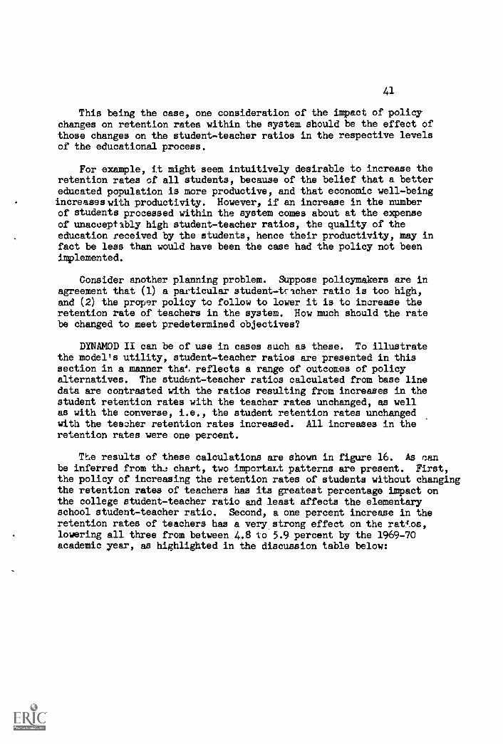
41
This being the case, one consideration of the impact of policychanges on retention rates within the system should be the effect ofthose changes on the student-teacher ratios in the respective levelsof the educational process.
For example, it might seem intuitively desirable to increase theretention rates of all students, because of the belief that a bettereducated population is more productive, and that economic well-beingincreases with productivity. However, if an increase in the numberof students processed within the system comes about at the expenseof unacceptably high student-teacher ratios, the quality of theeducation received by the students, hence their productivity, may infact be less than would have been the case had the policy not beenimplemented.
Consider another planning problem. Suppose policymakers are inagreement that (1) a particular student-tcacher ratio is too high,and (2) the proper policy to follow to lower it is to increase theretention rate of teachers in the system. How much should the ratebe changed to meet predetermined objectives?
DYNAMOD II can be of use in cases such as these. To illustratethe modelts utility, student-teacher ratios are presented in thissection in a manner the', reflects a range of outcomes of policyalternatives. The student-teacher ratios calculated from base linedata are contrasted with the ratios resulting from increases in thestudent retention rates with the teacher rates unchanged, as wellas with the converse, i.e., the student retention rates unchangedwith the teacher retention rates increased. All increases in theretention rates were one percent.
The results of these calculations are shown in figure 16. As canbe inferred from the chart, two important patterns are present. First,the policy of increasing the retention rates of students without changingthe retention rates of teachers has its greatest percentage impact onthe college student-teacher ratio and least affects the elementaryschool student-teacher ratio. Second, a one percent increase in theretention rates of teachers has a very strong effect on the rat7f.os,lowering all three from between 4.8 to 5.9 percent by the 1969-70academic year, as highlighted in the discussion table below:
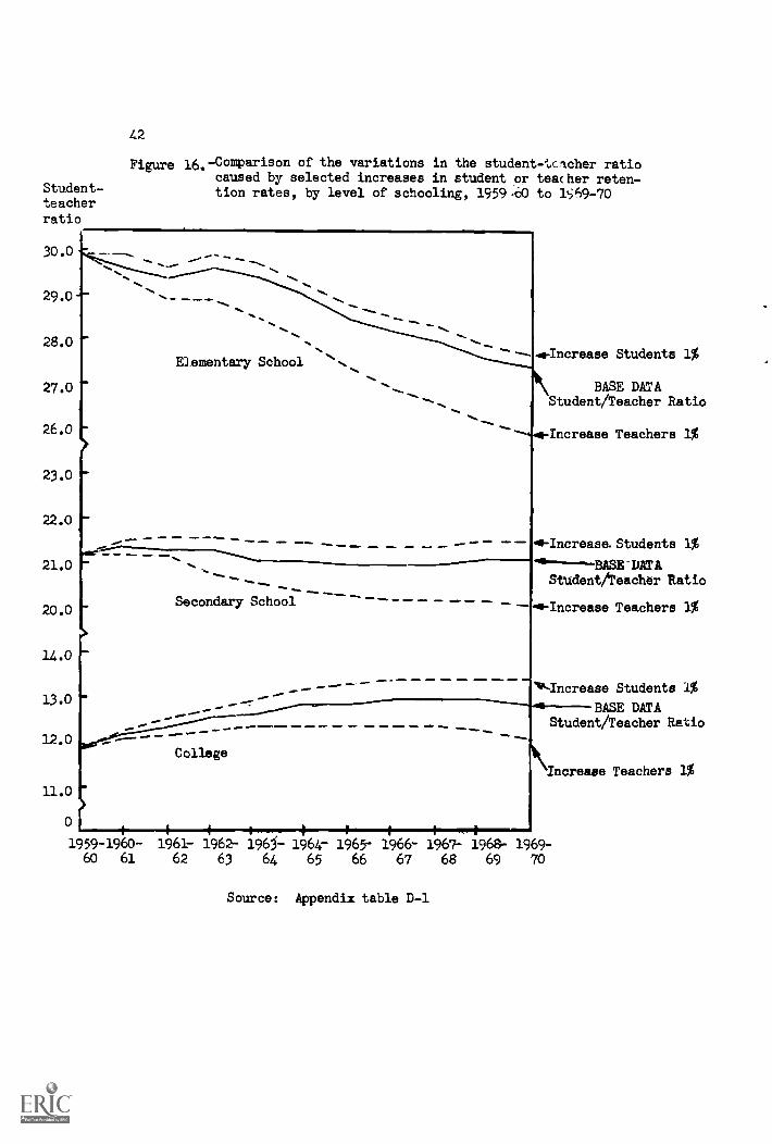
Student-teacherratio
30.0
29.0
28.0
27.0
26.0
23.0
22.0
21.0
20.0
14.0
13.0
12.0
11.0
0I I
1959-1960- 1961- 1962- 196j- 1964- 1965- 1966- 1967- 1968- 1969-60 61 62 63 64 65 66 67 68 69 70
42
Figure 16. -Comparison of the variations in the student-tcacher ratiocaused by selected increases in student or teacher reten-tion rates, by level of schooling, 1959.60 to 159-70
-
., ,Elementary School
=
=-Secondary School
College
48-Increase Students 1%
BASE DATAStudent/Teacher Ratio
.1-Increase Teachers 1%
40-Increase.Students 1%
BAZE bAILStudent/teacher Ratio
AF-Increase Teachers 1%
V.-Increase Students 1%
BASE DATAStudent/teacher Ratio
Increase Teachers 1%
Source: Appendix table D-1

43
An increase of one percentin the retention rate of:
Produces a percent difference inthe base line student-teacher ratioapproximately equal to:
1964- 1969-1261 1272
Elementary school students 1.3 1.3Secondary school students 1.7 2.1
College students 2.3 3.0
Elementary school teachers -3.7 -5.8Secondary school teachers -3.3 -4.8College teachers -3.5 -5.9
The data in appendix table D-1 indicate that, for the collegesector, either alternative of increasing the student retention rate orthe teacher retention rate by one percent will be associated with anabsolute increase in the student-teacher ratio over the middle rangeof the projection interval. This is a pure population effect causedby the enlarged college enrollments, and is sufficient to offset theeffects of small increases in the number of college teachers. Thissuggests that if the desired policy is ultimately to increase thenumber of students, in the system over the base line projections, oneway of minimizing the impact on the student-teacher ratio is tosequence the operations: first to pursue policies that will -etainmore teachers in the system, and then take the desired action toincrease the retention rates of students. (See "Policy sequencing"below).
Examining the data in more detail it can be noted that, even thoughmore students enter the system each year at the elementary school level,the projected number of elementary school teachers increases at a fasterrate than the students, lowering the student-teacher ratio from 29.9 in1959-60 to 27.8 in 1969-70. In the secondary school sector, littlechange is noted over the interval.
If a one-percent increase is made in the retention rates ofsecondary school students the relative difference in the student-teacherratio over the base line ratios is slightly greater than for the elemen-tary school sector. A one-percent increase in the retention rate forcollege students increases the student-teacher ratio from a base linevalue of 12.9 to 13.3 in the 1969-70 academic year.
For elementary school teachers, an increase of one percent in theirretention rate implemented in 1959-60 would have decreased the student -teacher ratio from 27.4 to about 25.9 by 1969-70.
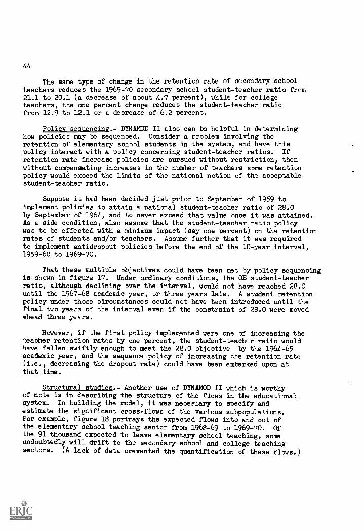
44
The same type of change in the retention rate of secondary schoolteachers reduces the 1969-70 secondary school student-teacher ratio from21.1 to 20.1 (a decrease of about 4.7 percent), while for collegeteachers, the one percent change reduces the student-teacher ratiofrom 12.9 to 12.1 or a decrease of 6.2 percent.
Policy sequencing.- DYNAMOD II also can be helpful in determininghow policies may be sequenced. Consider a problem involving theretention of elementary school students in the system, and have thispolicy interact with a policy concerning student-teacher ratios. Ifretention rate increase policies are Pursued without restriction, thenwithout compensating increases in the number of teachers some retentionpolicy would exceed the limits of the national notion of the acceptablestudent-teacher ratio.
Suppose it had been decided just prior to September of 1959 toimplement policies to attain a national student-teacher ratio of 28.0by September of 1964, and to never exceed that value once it was attained.As a side condition, also assume that the student-teacher ratio policywas to be effecteet with a minimum impact (say one percent) on the retentionrates of students and/or teachers. Assume further that it was requiredto implement antidropout policies before the end of the 10-year interval,1959-60 to 1969-70.
That these multiple objectives could have been met by policy sequencingis shown in figure 17. Under ordinary conditions, the OE student-teacherratio, although declining over the interval, would not have reached 28.0until the 1967-68 academic year, or three years late. A student retentionpolicy under those circumstances could not have been introduced until thefinal two yeas of the interval even if the constraint of 28.0 were movedahead three years.
However, if the first policy implemented were one of increasing theteacher retention rates by one percent, the student - teacher ratio wouldhave fallen swiftly enough to meet the 28.0 objective by the 1964-65academic year, and the sequence policy of increasing the retention rate(i.e., decreasing the dropout rate) could have been embarked upon atthat time.
Structural studies.- Another use of DYNAMOD II which is worthyof note is in describing the structure of the flows in the educationalsystem. In building the model, it was neces:5ary to specify andestimate the significant cross-flows of the various subpopulations.For example, figure 18 portrays the expected flows into and out ofthe elementary school teaching sector from 1968-69 to 1969-70. Ofthe 91 thousand expected to leave elementary school teaching, someundoubtedly will drift to the secondary school and college teachingsectors. (A lack of data Prevented the quantification of these flows.)
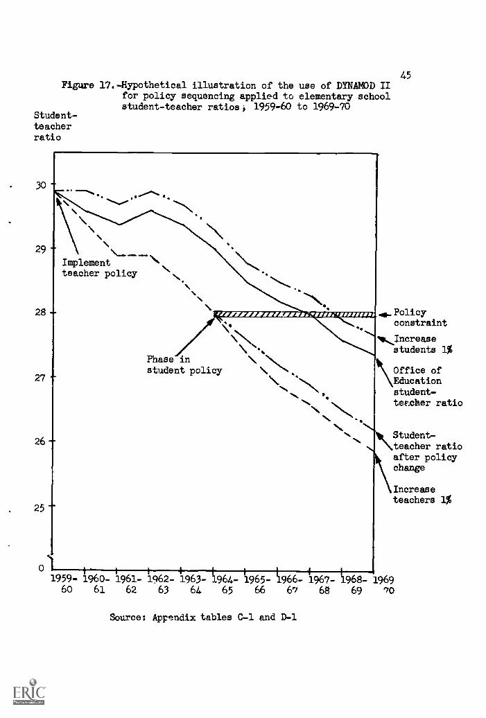
45Figure 17.-Hypothetical illustration of the use of DYNAMOD II
for policy sequencing applied to elementary schoolstudent-teacher ratios; 1959-60 to 1969-70
Student-teacherratio
29
Implement--\
teacher policy
28-
27-
26-
25
ilkZ=EEEZZIE
/ Ss\ N\ N..
\N\\ N\ p.
Phase instudent policy
constraint
NINIncreasestudents 1%
\Office ofEducationstudent-tetcher ratio
Nt Student -
\teacher ratioafter policychange
Increaseteachers 1%
01I
1959- 1960- 1961- 1962- 1963- C.964- 1965- 666- 1967- 11968- 196960 61 62 63 64 65 66 67 68 69 '70
Source: Appendix tables C-1 and D-1
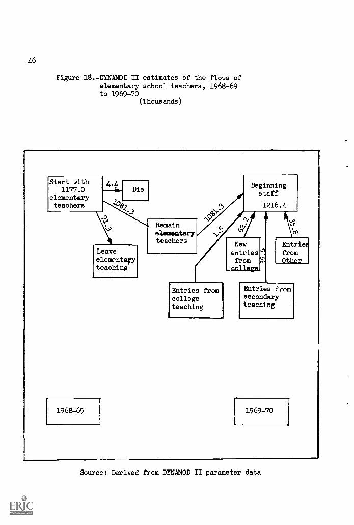
46
Figure 18.-DYNAMOD II estimates of the flows ofelementary school teachers, 1968-69to 1969-70
(Thousands)
Start with1177.0
elementaryteachers
L1968-69
Beginningstaff
1216.4
1 Remainelementaryteachers
rr)
Newentriesfrom
rnllaer
Entriea
fromOther
LeaveelemPntacyteaching
Entries fromcollegeteaching
Entries fromsecondaryteaching
1969-70
t
Source: Derived from DYNAMOD II parameter data
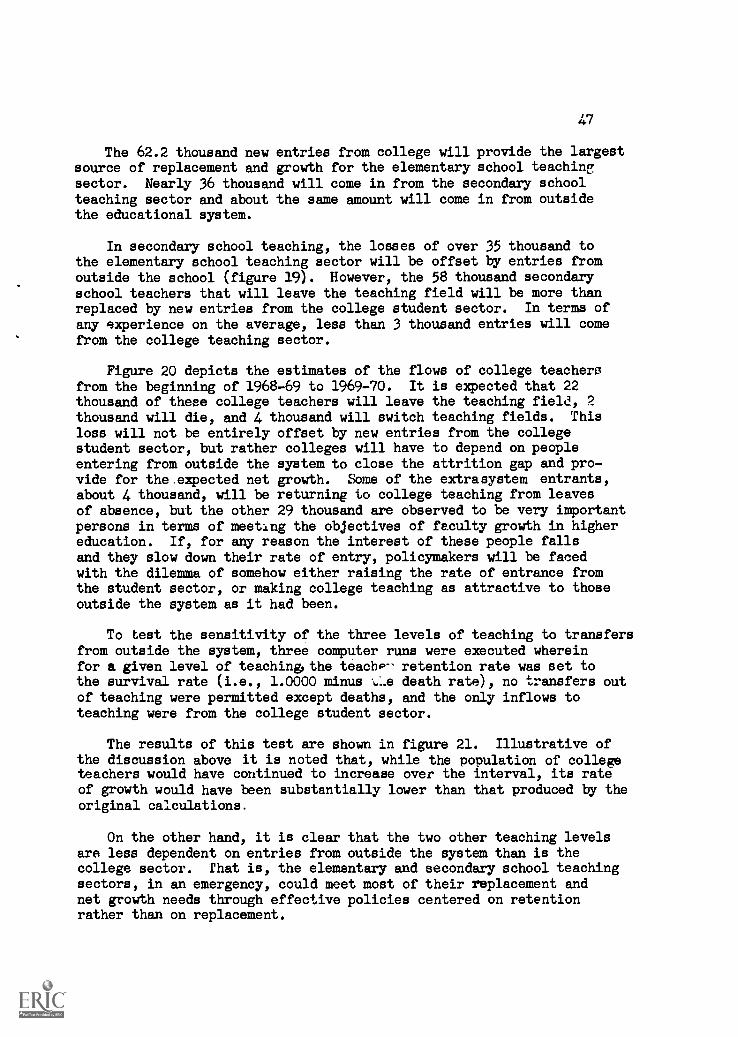
47
The 62.2 thousand new entries from college will provide the largestsource of replacement and growth for the elementary school teachingsector. Nearly 36 thousand will come in from the secondary schoolteaching sector and about the same amount will come in from outsidethe educational system.
In secondary school teaching, the losses of over 35 thousand tothe elementary school teaching sector will be offset by entries fromoutside the school (figure 19). However, the 58 thousand secondaryschool teachers that will leave the teaching field will be more thanreplaced by new entries from the college student sector. In terms ofany experience on the average, less than 3 thousand entries will comefrom the college teaching sector.
Figure 20 depicts the estimates of the flows of college teachersfrom the beginning of 1968-69 to 1969-70. It is expected that 22thousand of these college teachers will leave the teaching field, 2thousand will die, and 4 thousand will switch teaching fields. Thisloss will not be entirely offset by new entries from the collegestudent sector, but rather colleges will have to depend on peopleentering from outside the system to close the attrition gap and pro-vide for the expected net growth. Some of the extrasystem entrants,about 4 thousand, will be returning to college teaching from leavesof absence, but the other 29 thousand are observed to be very importantpersons in terms of meeting the objectives of faculty growth in highereducation. If, for any reason the interest of these people fallsand they slow down their rate of entry, policymakers will be facedwith the dilemma of somehow either raising the rate of entrance fromthe student sector, or making college teaching as attractive to thoseoutside the system as it had been.
To test the sensitivity of the three levels of teaching to transfersfrom outside the system, three computer runs were executed whereinfor a given level of teaching, the teachP- retention rate was set tothe survival rate (i.e., 1.0000 minus death rate), no transfers outof teaching were permitted except deaths, and the only inflows toteaching were from the college student sector.
The results of this test are shown in figure 21. Illustrative ofthe discussion above it is noted that, while the population of collegeteachers would have continued to increase over the interval, its rateof growth would have been substantially lower than that produced by theoriginal calculations.
On the other hand, it is clear that the two other teaching levelsare less dependent on entries from outside the system than is thecollege sector. that is, the elementary and secondary school teachingsectors, in an emergency, could meet most of their replacement andnet growth needs through effective policies centered on retentionrather than on replacement.
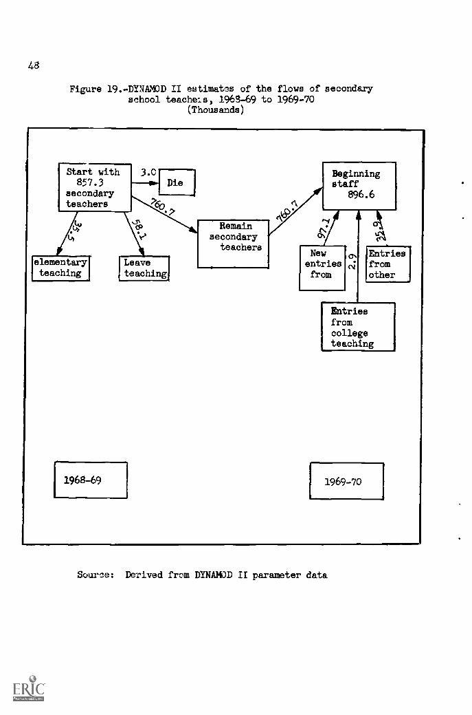
48
Figure 19.-DYNAMOD II estimatos of the flows of secondaryschool teachers, 1963 -69 to 1969-70
(Thousands)
Start with857.3
secondaryteachers
DieBeginningstaff
896.6
11
Remainsecondaryteachers
Newentriesfrom
rn Entriesfromother
elementaryteaching
Leaveteaching
1968-69
Entriesfromcollegeteaching
1969-70
Sour e: Derived from DYNAMOD II parameter data
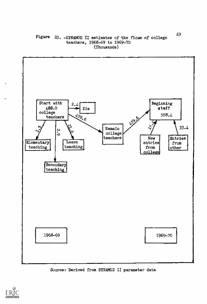
Figure 20. -DYNAMOD II estimates of the flows of collegeteachers, 1968-69 to 1969-70
(Thousands)
49
Start with
488.0college
teachers
i
Elementaryteaching
Beginningstaff
508.4
crRemaincollege
teachers New EntriesLeave entries fromteaching from
college,other
Secondary
1968-69 1969-70
Source: Derived from DYNAMOD II parameter data
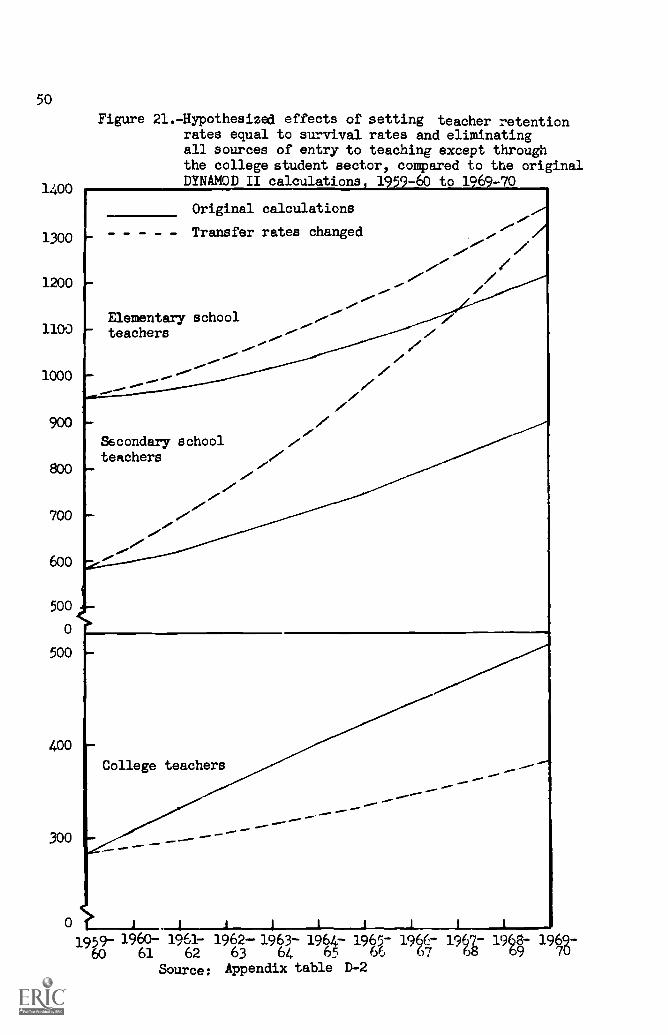
50
1400
1300
1200
1100
1000
900
700
600
500
0
500
400
300
0
Figure 21.-Hypothesized effects of setting teacher retentionrates equal to survival rates and eliminatingall sources of entry to teaching except throughthe college student sector, compared to the originalDYNAMOD II calculations, 1959-60 to 1969-70
Original calculations
Transfer rates changed
Elementary schoolteachers
Secondary schoolteachers
.1
College teachers
..
1959- 1960- 1961- 1962-1963- 1964- 1965- 1966- 1967- 1968- 1969-60 61 62 63 64 65 66 67 68 69 70
Source: Appendix table D-2
51
Limitations of the Data
The data are subject to all the limitations published elsewhereby the Office of Education and, where applicable, the Bureau of theCensus. The basic data inputs are derived primarily from the Bureauof the Census' 1/1,000 samples data tape, and hence are subject tosampling errors which become relatively larger as the population issubdivided in more detail. Efforts were made to adjust known dif-ferences, but these efforts cannot be considered to be completelyeffective.
For this report, the greatest effort was expended on calibratingto the major educational population categories (elementary schoolstudents, secondary school students, and so on). Therefore, onlysecondary emphasis was placed on the sex, race and age distributionswithin the entire population.
52
APPENDIX A
Summary calculations of DYNAMOD II
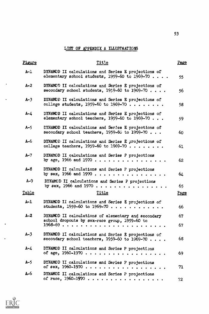
53
LIST OF APPENDIX A ILLUSTRATIONS
Figure Title Page
DYNAMOD II calculations and Series E projections ofelementary school students, 1959-60 to 1969-70 . . . . 55
A-2 DYNAMOD II calculations and Series E projections ofsecondary school students, 19;9-60 to 1969-70 . . . . 56
A-3 DYNAMOD II calculations and Series E projections ofcollege students, 1959-60 to 1969-70 58
A -4 DYNAMOD II calculations and Series E projections ofelementary school teachers, 1959-60 to 1969-70 . . . 59
A -5 DYNAMOD II calculations and Series E projections ofsecondary school teachers, 1959-60 to 1969-70 . . . 60
A-6 DYNAMOD II calculations and Series E projections ofcollege teachers, 1959-60 to 1969-70 61
A-7 DYNAMOD II calculations and Series P projectionsby age, 1966 and 1970 62
A-8 DYNAMOD II calculations and Series P projectionsby sex, 1966 and 1970 64
A-9 DYNAMOD II calculations and Series P projectionsby sex, 1966 and 1970 65
Table Title Page
A-1 DYNAMOD II calculations and Series E projections ofstudents, 1959-60 to 1969-70 66
A-2 DYNAMOD II calculations of elementary and secondary 67school dropouts by sex-race group, 1959-60 to1968-69 67
A-3 DYNAMOD II calculations and Series E projections ofsecondary school teachers, 1959-60 to 1969-70 . . . . 68
A-4 DYNAMOD II calculations and Series P projectionsof age, 1960-1970 69
A -5 DYNAMOD II calculations and Series P projectionsof sex, 1960-1970 71
A-6 DYNAMOD II calculations and Series P projectionsof race, 1960-1970 72
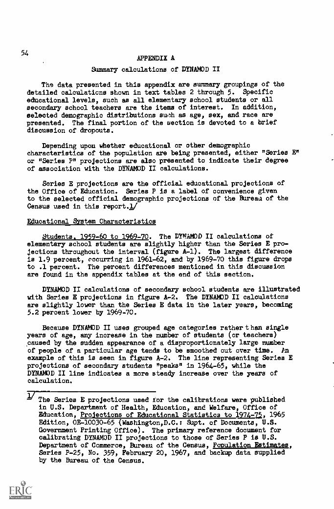
54APPENDIX A
Summary calculations of DYNAMOD II
The data presented in this appendix are summary groupings of thedetailed calculations shown in text tables 2 through 5. Specificeducational levels, such as all elementary school students or allsecondary school teachers are the items of interest. In addition,selected demographic distributions su,:h as age, sex, and race arepresented. The final portion of the section is devoted to a briefdiscussion of dropouts.
Depending upon whether educational or other demographiccharacteristics of the population are being presented, either "Series E"or "Series P" projections are also presented to indicate their degreeof association with the DYNAMOD II calculations.
Series E projections are the official educational projections ofthe Office of Education. Series P is a label of convenience givento the selected official demographic projections of the Bureau of theCensus used in this report.1/
Educational System Characteristics
Students. 1959-60 to 1969-70. The DYNAMOD II calculations ofelementary school students are slightly higher than the Series E pro-jections throughout the interval (figure A -i). The largest differenceis 1.9 percent, occurring in 1961-62, and by 1969-70 this figure dropsto .1 percent. The percent differences mentioned in this discussionare found in the appendix tables at the end of this section.
DYNAMOD II calculations of secondary school students are illustratedwith Series E projections in figure A-2. The DYNAMO]) II calculationsare slightly lower than the Series E data in the later years, becoming5.2 percent lower by 1969-70.
Because DYNAMOD II uses grouped age categories rather than singleyears of age, any increase in the number of students (or teachers),caused by the sudden appearance of a disproportionately large numberof people of a particular age tends to be smoothed out over time. Anexample of this is seen in figure A-2. The line representing Series Eprojections of secondary students "peaks" in 1964-65, while theDYNAMOD II line indicates a more steady increase over the years ofcalculation.
The Series E projections used for the calibrations were publishedin U.S. Department of Health, Education, and Welfare, Office ofEducation, Projections of Educational Statistisstoo1271:71, 1965Edition, 0E-10030-65 (Washington,D.C.: Supt. of Documents, U.S.Government Printing Office). The primary reference document forcalibrating DYNAMOD II projections to those of Series P is U.S.Department of Commerce, Bureau of the Census, Population Estimates,Series P -25, No. 359, February 20, 1967, and backup data suppliedby the Bureau of the Census.
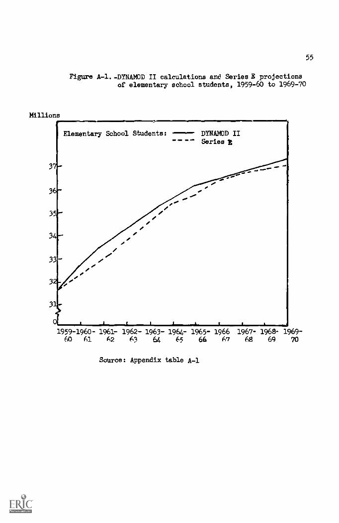
Figure A-1.-DYNAMOD II calculations and Series E projectionsof elementary school students, 1959-60 to 1969-70
Millions
37,
3
35
33
3
Amawo......IIMM'.,SS:
Elementary School Students: DYNAMOD II-- Series
1.= "1959-1960- 1961- 1962- 1963- 1964- 1965- 1966 1967- 1968- 1969-60 61 62 63 64 65 66 67 68 69 70
Source: Appendix table A-1
55

56
Figure A-2. -DYNAMOD II calculations and Series E. projectionsof secondary school students, 1959-60 to 1969-70
Millions
15
14
13
12
11
10
9
0
1959-60
1960-61
1961-62
1962-63
1963-64
1964-65
1965-66
1966-67
1967-68
1968-69
1969-70
Source: Appendix table A-1
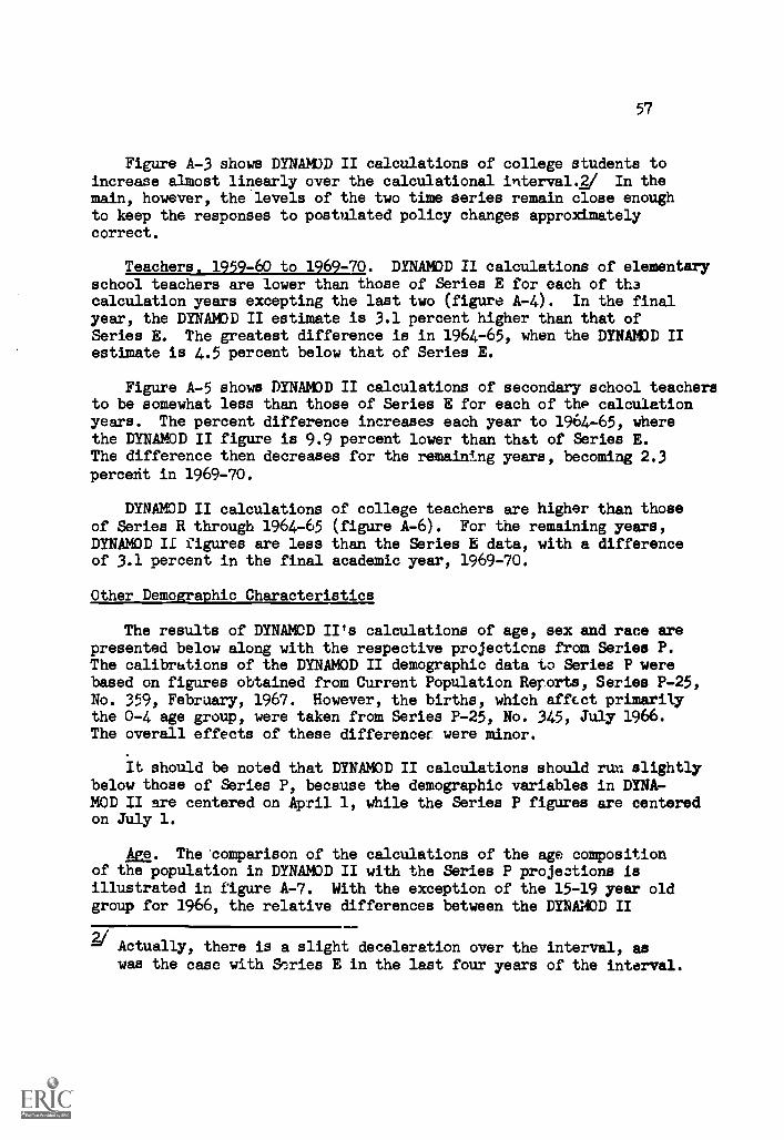
57
Figure A-3 shows DYNAMO]) II calculations of college students toincrease almost linearly over the calculational interval .a/ In themain, however, the levels of the two time series remain close enoughto keep the responses to postulated policy changes approximatelycorrect.
Teachers. 1959-60 to 1969-70. DYNAMOD II calculations of elementaryschool teachers are lower than those of Series E for each of thacalculation years excepting the last two (figure A-4). In the finalyear, the DYNAMOD II estimate is 3.1 percent higher than that ofSeries E. The greatest difference is in 1964-65, when the DYNAMO]) IIestimate is 4.5 percent below that of Series E.
Figure A-5 shows DYNAMOD II calculations of secondary school teachersto be somewhat less than those of Series E for each of the calculationyears. The percent difference increases each year to 1964-65, wherethe DYNAMOD II figure is 9.9 percent lower than that of Series E.The difference then decreases for the remaining years, becoming 2.3percent in 1969-70.
DYNAMOD II calculations of college teachers are higher than thoseof Series R through 1964-65 (figure A-6). For the remaining years,DYNAMOD II figures are less than the Series E data, with a differenceof 3.1 percent in the final academic year, 1969-70.
Other Demographic Characteristics
The results of DYNAMOD II's calculations of age, sex and race arepresented below along with the respective projections from Series P.The calibrations of the DYNAMOD II demographic data to Series P werebased on figures obtained from Current Population Reports, Series P-25,No. 359, February, 1967. However, the births, which affect primarilythe 0-4 age group, were taken from Series P-25, No. 345, July 1966.The overall effects of these differences were minor.
It should be noted that DYNAMOD II calculations should run slightlybelow those of Series P, because the demographic variables in DYNA-MOD II are centered on April 1, while the Series P figures are centeredon July 1.
Am. The oomparison of the calculations of the age compositionof the population in DYNAMOD II with the Series P projections isillustrated in figure A-7. With the exception of the 15-19 year oldgroup for 1966, the relative differences between the DYNAMOD II
2/ Actually, there is a slight deceleration over the interval, aswas the case with Series E in the last four years of the interval.
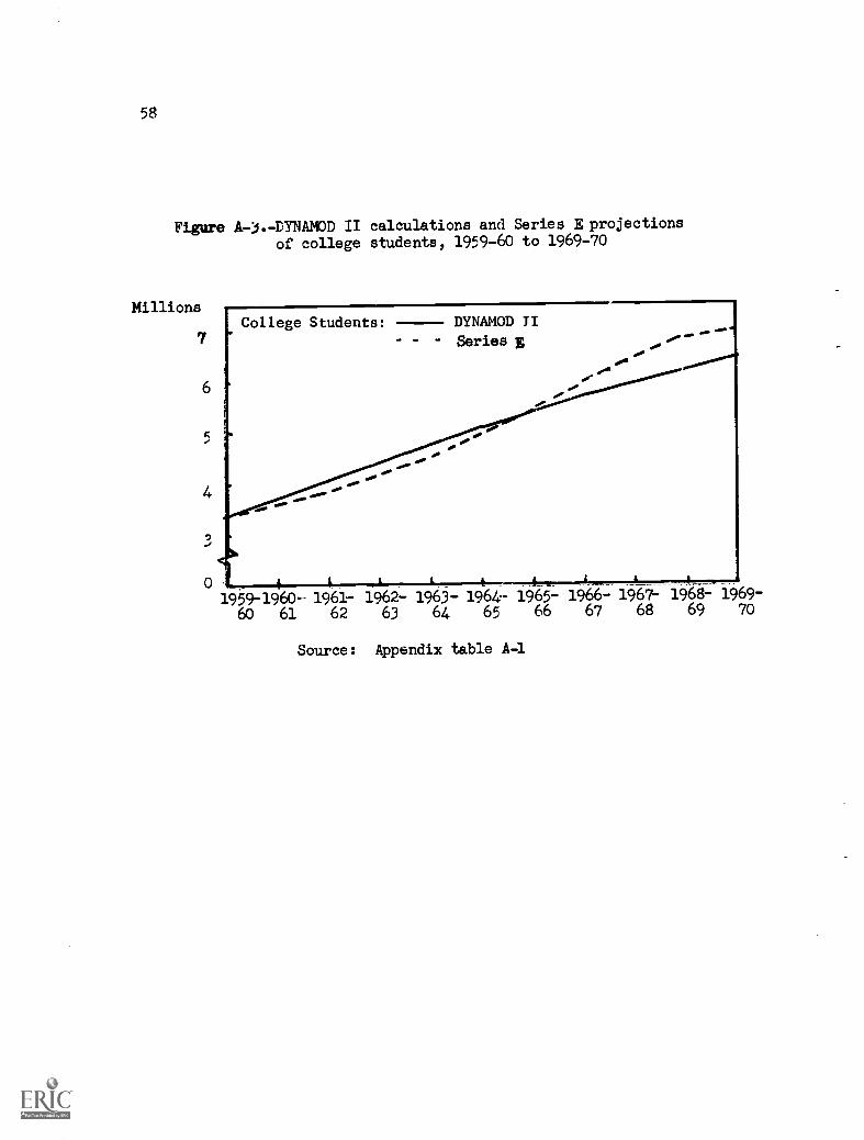
58
Figure A,.3.-DYNAMOD II calculations and Series E projectionsof college students, 1959-60 to 1969-70
Millions
7College Students: DYNAMOD TI
Series E
.00
0 4 .' "_.
1959- 1960-- 1961- 1962- 1963- 1964- 196-60 61 62 63 64 65 66
Source: Appendix table A-1
1966- 1967- 1968- 1969 -
67 68 69 70
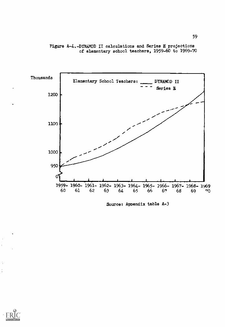
59
Figure A-4.-DYNAMOD II calculations and Series E projectionsof elementary school teachers, 1959-60 to 1969-70
ThousandsElementary School Teachers: DYNAMOD II
Series E
1959- 1960- 1961- 1962- 1963- 1964- 1965- 1966- 1967- 1968- 196960 61 62 63 64 65 66 67 68 69 70
Source: Appendix table A-3
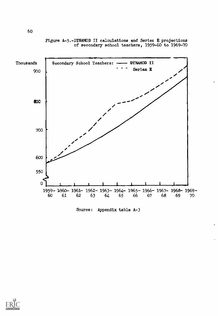
60
Figure A-5.-DYNAMOD II calculations and Series E projectionsof secondary school teachers, 1959-60 to 1969-70
Thousands Secondary School Teachers: DYNAMOD II
Series E900
800
700
550
0 _I
1959- 1960- 1961- 1962- 1963- 1964- 1965- 1966- 1967- 1968- 1969 -
60 61 62 63 64 65 66 67 68 69 70
Source: Appendix table A-3
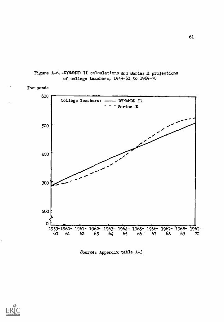
Figure A-6.-DYNAMOD II calculations and Series I projections
of college teachers, 1959-60 to 1969-70
Thousands
600
500
400
300
200
0
College Teachers: ----- DYNAMOD II
Series
61
1959-1960-60 61
1961-62
1962-
63
1963-
641964-
651965-66'
1966-67
1967-68
1968-69
.1969-
70
Source; Appendix table A-3
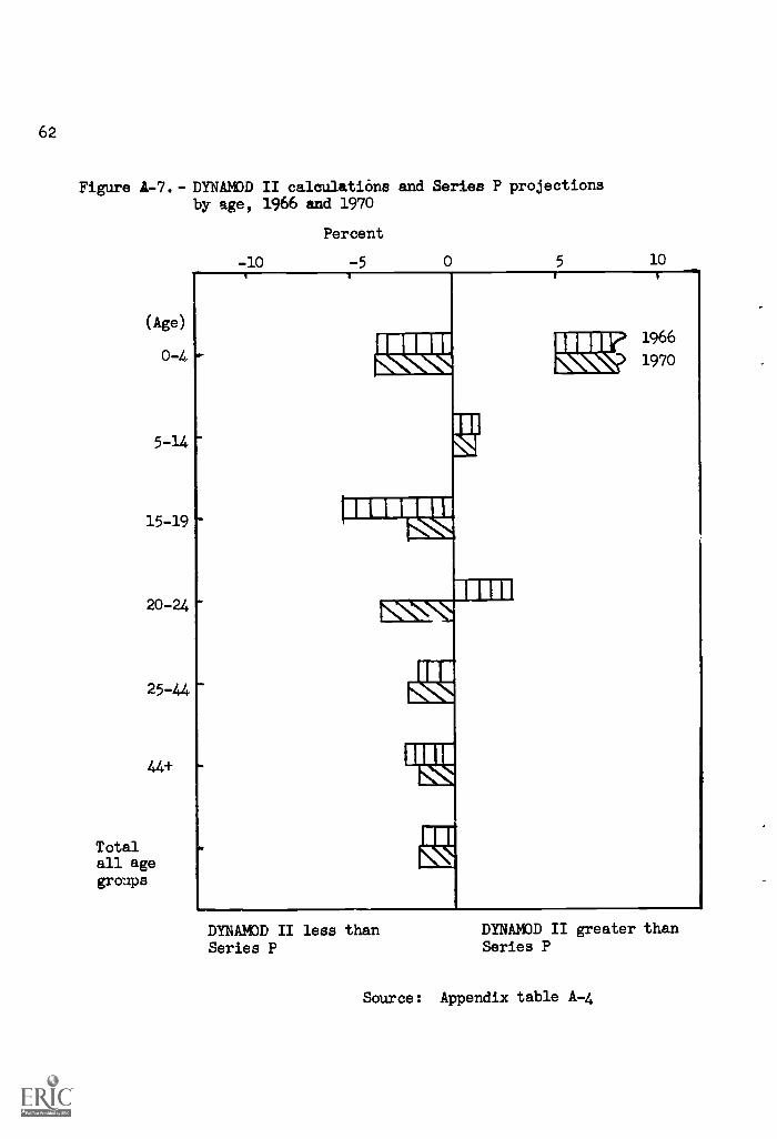
62
Figure A-7. - DYNAIIDD II calculations and Series P projectionsby age, 1966 and 1970
(Age)
0-4
5-14
15-19
20-24
25-44
44+
Totalall agegroups
Percent
-10 -5 0 5 10
BLS
1966
1970
DYNAMOD II less than DYNAMOD II greater than
Series P Series P
Source: Appendix table A-4
63
calculations and those in Series P all were less than 4 percent.
The relative deviations tend to be largest ir. the younger agegroups. In addition, with the exception of the 5-14 year old group,DYNAMOD II calculations tend to be slightly lower than Series P.
Sex. Figure A-8 shows DYNAMOD II calculations by sex for theyears 160, 1966, and 1970. For males, the DYNAMO') II 1970 calculationsis 1.5 percent less than the Series P projection, while for femalesthe difference is 1.6 percent.
Race . A graphic comparison of DYNAMOD II calculations andSeries P projections by race is shown in figure A-9. For whites, theDYNAMOD II calculation is 1.0 percent below Series P in 1966, be-coming 1.6 percent below in 1970. For nonwhites, DYNAMOD II is only.8 percent lower than Series P in 1966, drifting to -1.2 percent by1970.
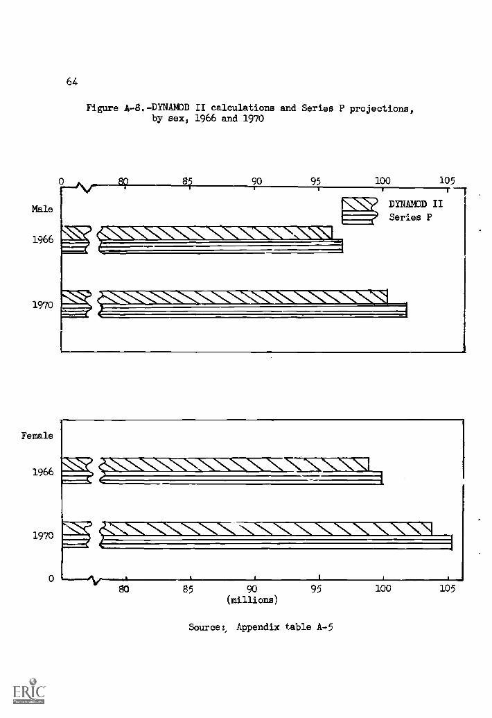
Male
1966
1970
Female
1966
1970
64
Figure A-8. -DYNAMO II calculations and Series P projections,by sex, 1966 and 1970
Et 90 95 100 105
DYNAMOD II
Series P
SEIM..\\46... '41b111L.N1111161111111
080 85 90
(millions)95
Source:, Appendix table A-5
100 105
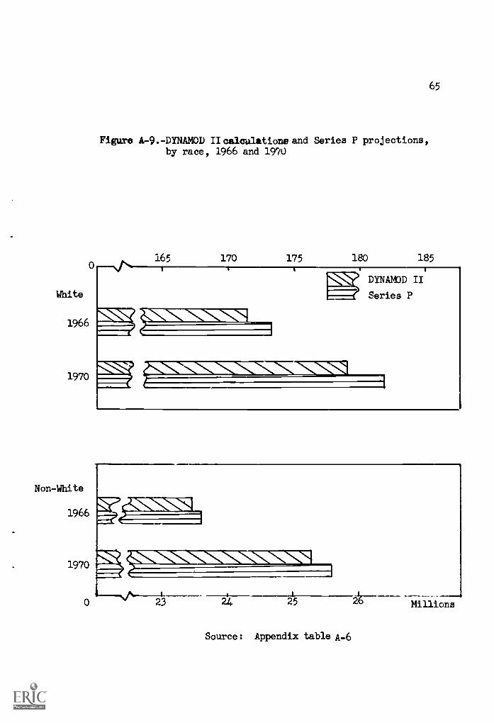
White
1966
1970
Non-White
1966
1970
Figure A-9.-DYNAMOD II calculations and Series P projections,by race, 1966 and 1970
165 170 175 180
65
185
DYNAMOD II
Series P
Source: Appendix table A-6
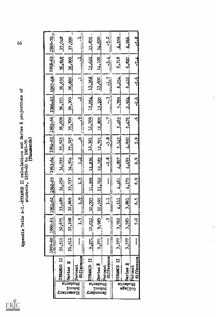
Appendix Table. A-1.-DYNAMOD II calculations and Series E projections of
students, 1959-60 to 1969-70
(Thousands)
4343
1-1
0o
43
CD
.00
! difference
---
1.5
I
CO
Percent
DYNAMD II
Series E
1959-60
1960-61
31,511
31,511
1961-62
32,675
33,489
32,198
I32,869
1.9
DYNAMD II
9,271
10,012
10.707
Series E
9,271
I_
9,983
10,595
Percent
difference
.3
1.1
m DYNAMOD II
+,
tto o
rt.S Series E
ri 8rercent
difference
3,377
3,762
3,377
3,583
4,111
3,86
1
962-63
11961-64
34,252
I34,935
33,737
34,504
1.2
1.5
11
0
11,312
- -
-
11,83_6_
12 183
-2.8
5.0
6.5
4,461
I4,807
4,175
4,495
6.9
6.9
o.
19_64=0_
19.61-661_1966-67
36,009
1967,68,
36,635
1968-69
36,448
1969-74
I
'1048
37,000
35,525
35,325
362.371
36,300
35,700
36,600
36,800
.6
.2
,1.1
.1
12,301
12,709
13,064
13,368
13,622
_33,835_
1201
12,800
13.100
13,600
14,100
14,600
-3.8
-.3
-1.7
_
5t143
5.29
6,054
.64318
6,559
42950
5,435
.5.924
6,410
6,820
6,966
3.9
.6
-2.6
-5.6
-7.4
-.8
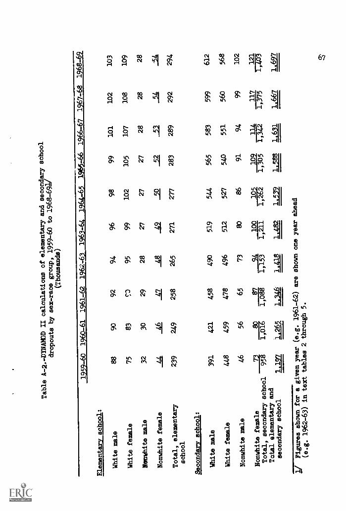
Table A-2.ZYNAMOD II calculations of elementary
and secondary school
dropouts by sex-race group, 1959-60 to
1968-691/
(Thousands)
1959-60
1960-611961-62 1962-616-616-61-6261.266=68-6
Elementary school:
White male
88
90
92
94
96
98
99
101
102
103
White female
75
83
cO
95
99
102
105
107
108
109
Nonwhite male
32
30
29
28
27
27
27
28
28
28
Nonwhite female
AA
Ak
42
19
1R
12
_14
J.&
Total, elementary
school
239
249
258
_4g
265
_42
271
277
283
289
292
294
Secondary school:
White male
391
421
458
490
519
544
565
583
599
612
White female
448
459
478
496
512
527
540
551
560
568
Nonwhite male
46
56
65
73
80
86
91
94
99
102
Nonwhite female
73
80
87
9A
100
105
109
114
117
121
Total, secondary school
958
1,61 g
1,088
1,153
1,211
1,262
1,305
1,342
1,375
1,403
Total elementary and
secondary school
1.197
1,265
1.346
1.418
1.482
1,539
1,588
1,631
1,667
1.697
Figures shown for a given year
(e.g. 1961-62) are shown one year ahead
(e.g. 1962-63) in text tables 2 through 5.
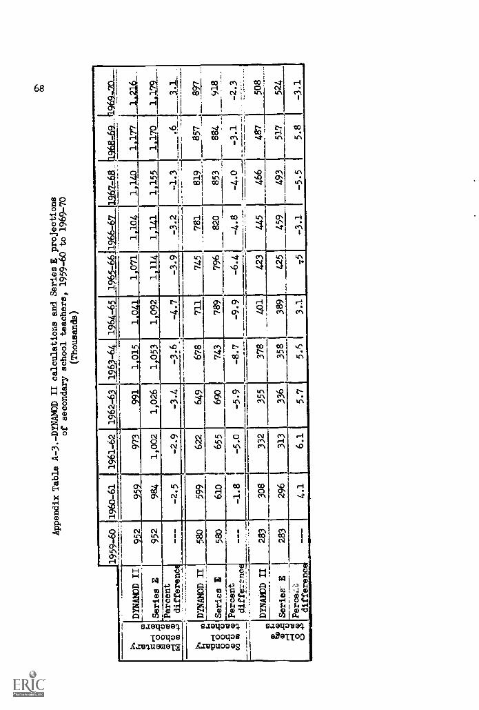
Appendix Table A-3.-DYNAMOD II calculations and Series E. projections
of secondary school teachers, 1959-60 to 1969-70
(Thousands)
1959-60
1960-61
1961-62
1962-63
1963-64
16 -6
1965-66
1966-67
1267-68
1.177
969.20_
I.3
SI
I 8 '
0 .0 g
I-I
0 0
w 0
+3
DYNAMOD II
952
952_]
973
991
1.015
1 0 1
1 071
1,104
1,,
1,216
1 179_
3.1
897
Series P.;
952
984
1,002
1,026
-3.4
1,053
-3.6
1 092
1 114
-4.7
-3.9
1,141
I
-3.2
1,155
1.170
Percent
difference
-2.5
-2.9
-1.3
819
1
.6
1
857
tb 0
2 0g 8 11
o.cd
0 o 0
C/3
03 +
3 00
$400
00
4ri
alo 0
C) 4"
DYNAMOD II
580
599
622
649
678
711
745
781
series E
580
610
655
690
743
789
796
820
-4.8
445
853
-4.0
......
884
-3.1
487
918
-2.3
508
Percent
diffene
zz
DYNAMOD II
---
-1.8
-5.0
-5.9
-8.7
-9.91
-6.4
283
308
332
355
378
401
423
466
Series E
Perce-L
difference;
283
296
313
336
358
389
425.
459
493
517
524
i
4.1
6.1
I5.7
5.'S
3.1
75
-3.1
-5.5
5.8
-3.1
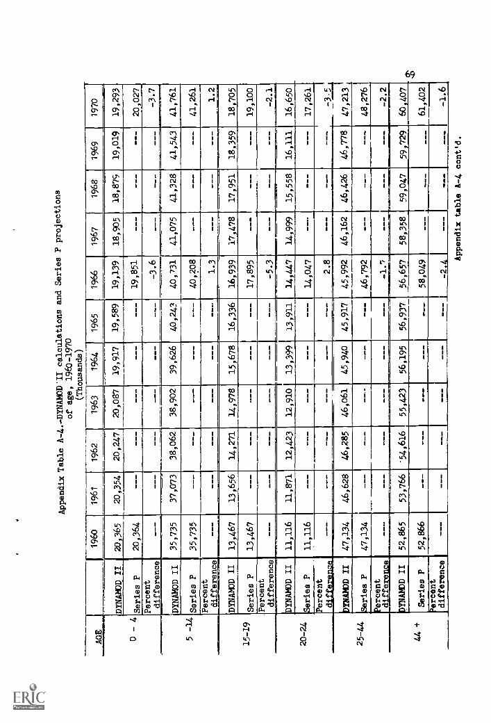
Appendix Table A-4.-DYNAMOD'II calculationsand Series P projections
of age, 196D-1970
(Thousands)
AGE1
1960
1961
1962
1963
1964
1965
1966
1967
1968
1969
1970
DYNAMOD II
20,365
20,354
20,247
20,087
19,917
19,589
19,139
18,905
18,875
19,019
19,293
04Series P
20,364
- --
--_
- --
19,851
- --
---
20,027
Percent
difference
---
-3.6
-__
-3.7
5 -14
DYNAMOD II
35,735
37,073
38,062
38,902
39,626
40,243
40,731
41,075
41,328
41,543
41,761
Series P
35,735
- --
- --
40,208
---
41,261,
Percent
difference
---
---
---
-1.3
---
1.2
15-19
DYNAMOD II
13,467
13,656
14,271
14,978
15,678
16,336
16,939
17,478
17,951
18,359
18,705
Series P
13,467
- --
- --
._
17,895
- --
- --
19,100
Percent
difference
- --
- --
-5.3
___
-__
-2.1
20-24
DYNAMOD II
11,116
11,871
12,423
12,910
13,399
13,911
14,447
14,999
15,558
16,111
16,650
Series P
11,116
---
---
14,047
___
---
17,261
Percent
different:
---
_--
--_
2.8
---
___
___
25-44
DYNAMOD II
47,134
46,628
46,285
46,061
45,940
45,917
45,992
46,162
46,426
46,778
47,213[
/Series P
47,134
- --
- --
- -'-
---
46,792
- --
- --
---
48,2761
Percent
diffevnce
---
---
---
---
-1.!
---
---
---
-2.2
44 +
DYNAMOD II
52,865
53,766
54,616
55,423
56,195
56,937
56,657
58,358
59,047
59,729
60,407
Series P
52,866
---
---
58,049
61,402
'ercent
difference
---
---
---
---
-24
- --
- --
---
-1.6
Appendix table A-4 cont'd.
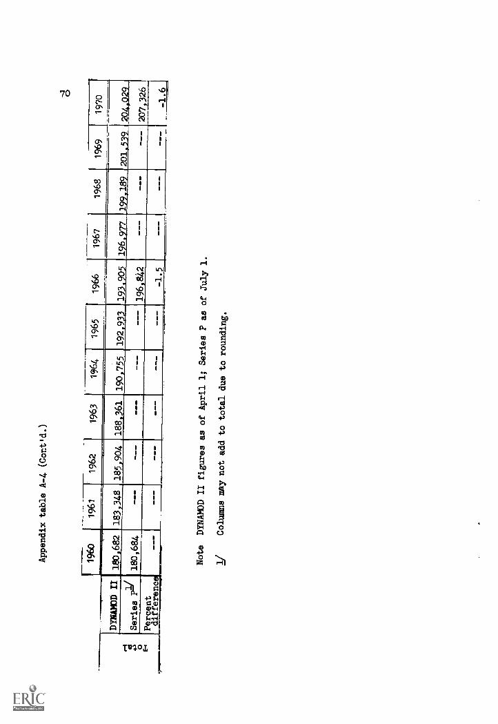
Appendix table A-4 (Contid.)
0
1960
1961
1962
1963
1964
1965
1966
1967
1968
1969
1970
.r1.43 o E
"
DYNAWD II
180,682
183,348
185,904
188,361
190,755
192,933
193,905
196.977
199,189
---
_i
201,539
---
204,029
207,326
Series
Pl/
180,684
---
---
_--
---
---
196,842
---
Percent
difference
---
---
---
---
---
---
-1.5
___
___
---
-1.6
Note DYNANOD II figures as ofApril 1; Series P as of July 1.
1/
Columns may not add to total due to
rounding.
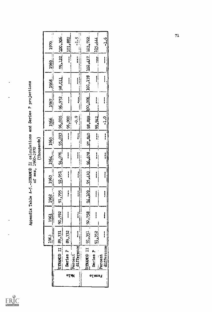
Appendix Table A-5.-DYNAMOD II calculations and Series P projections
of sex, 1960-1970
(Thousands)
1963
i1961
I1962
1963_
I1964
1965
I19_66
[1967
1968
I1969_
1970
DINAMOD II
89,331
90,592
91,795
92 951
94 076
95.093
96,005
96,972
98,011
99,12. 1004306._
Series P
89,332
---
96,900
41
___
___
---
---
---
2,21,882
MPercent
-0.9
-1.5
difference
---
--r_-
DYNAMO]) II
91 351
Series P
Percent
difference
92,758
194,109
---
I
_55,4101_96.678 _22,240 _98,899
9949
4LL
---1
.0
101,178
1a2.00.2_ 103,722_ _
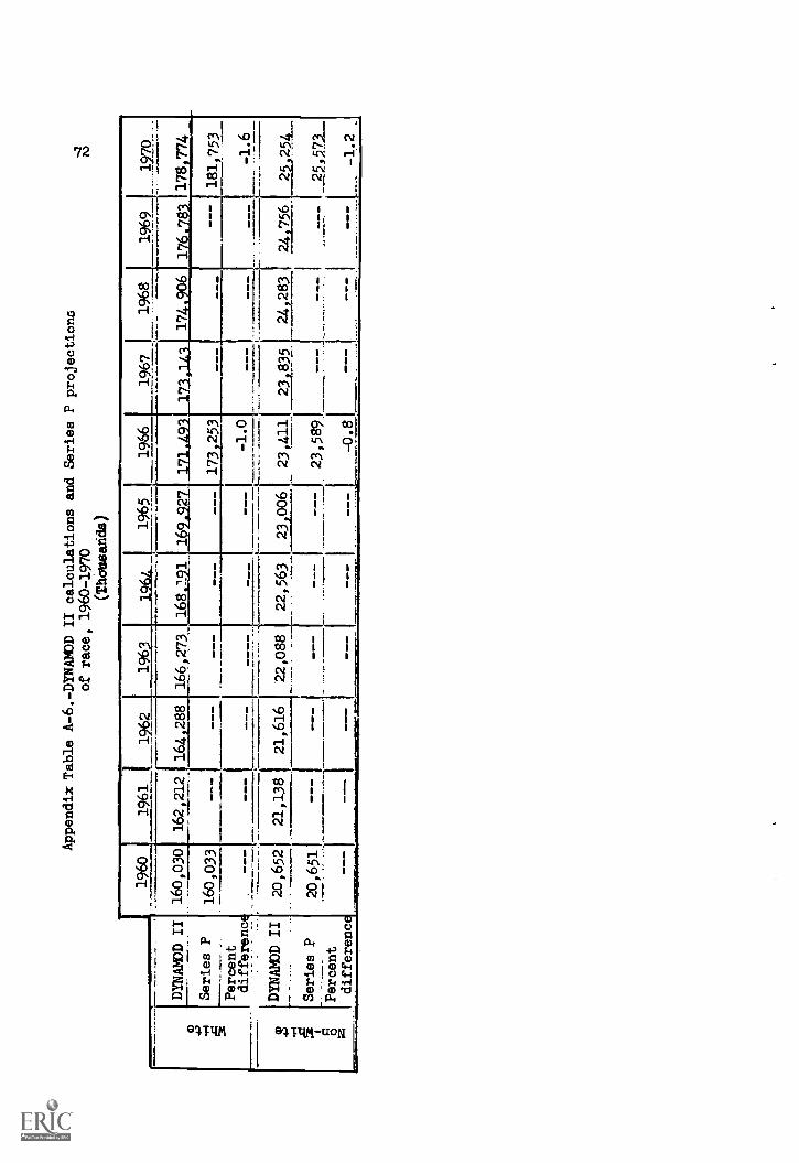
Appendix Table A-6.-DYNAMOD II calculations and Series P projections
of race, 1960-1970
(ThOugarida)
1960
1961
11962
1961
1965
1966
1967
1968
1969
1970
mt---
,-,
DYNAMO II
Series P
Percent
difference,
DYNAMO II
Series P
Percent
difference
160,030
162,212
164,288
166,273
---
168 1 1
16
17
17
06
176
8178,774
160
P033
- --
__-
-_-
-173 253
181,753
---
--1.0
---
-__
-1.6
k__
4 0 z
20,652
21,1381. =7=
21,616
22,088
---
--_
22,563
--
---
r 23,006r
23,4111
23,589
-O.
23,835
24,283
24,756.
__.7-
-7.7_
25,25.4_
_25,5_73_
-1.2
20,651
.__.._
- --I
- --
---
_--
- --
- - -
---
ii
73
APPENDIX B
Tables of the Effects of Using Different Birth Estimates
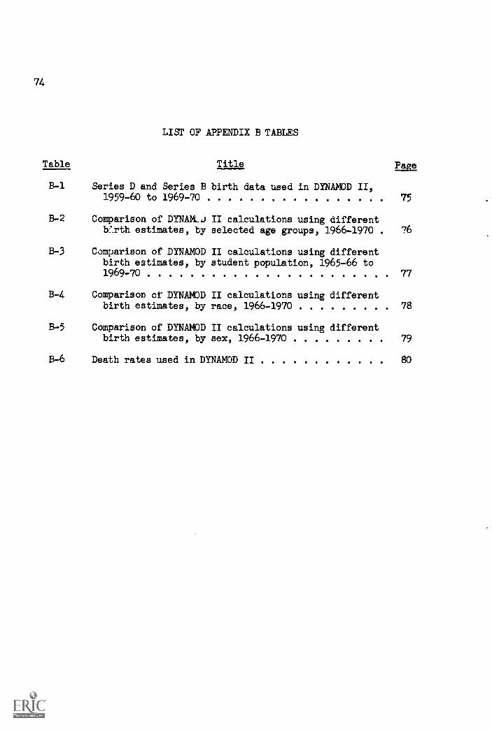
74
Table
B-1
B-2
B-3
B-4
B-5
B-6
LIST OF APPENDIX B TABLES
Title Page
75
selected age groups, ].966 -1970 76
Series D and Series B birth data used in DYNAMOD II,1959-60 to 1969-70
Comparison of DYNAM...Jb'.rth estimates, by
Comparison of DYNAMODbirth estimates, by1969-70
Comparison. of DYNAMODbirth estimates, by
Comparison of DYNAMODbirth estimates, by
II calculations using different
II calculations using differentstudent population, 1965-66 to
77
II calculations using differentrace, 1966-1970 78
II calculations using differentsex, 1966-1970 79
Death rates used in DYNAMOD II 80
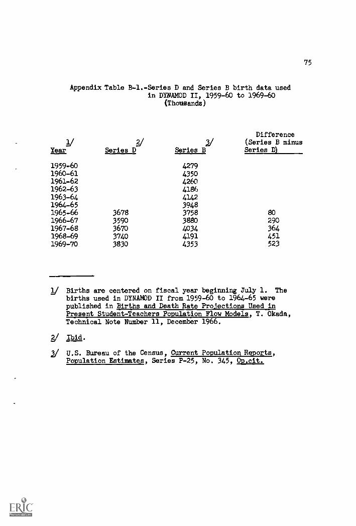
75
Appendix Table B-1.-Series D and Series B birth data usedin DYNAMOD II, 1959-60 to 1969-60
(Thousands)
1/Year
2/Series D
2/Series B
Difference(Series B minusSeries D)
1959-60 42791960-61 43501961-62 42601962-63 41861963-64 41421964-65 39481965-66 3678 3758 801966-67 3590 3880 2901967-68 3670 4034 3641968-69 3740 4191 4511969-70 3830 4353 523
1/ Births are centered on fiscal year beginning July 1. Thebirths used in DYNAMOD II from 1959-60 to 1964-65 werepublished in Births and Death Rate Projections Used inPresent Student-Teachers Population Flow Models, T. Okada,Technical Note Number 11, December 1966.
2/ Ibid.
1/ U.S. Bureau of the Census, Current Population Reports,Population Estimates, Series P-25, No. 345, OP.cit.
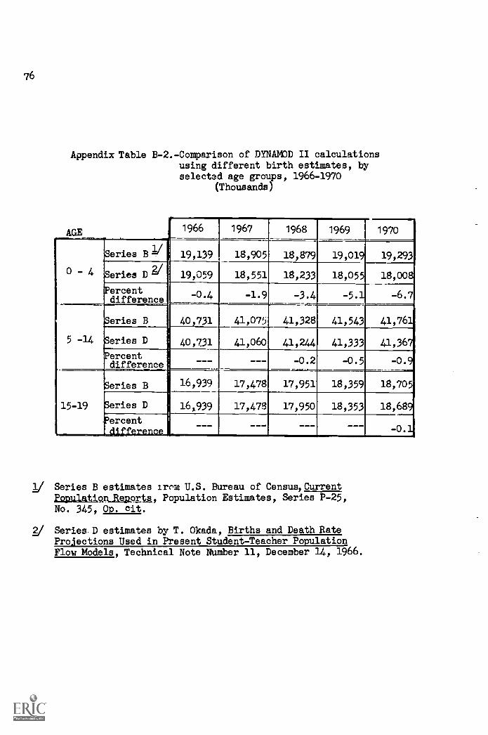
76
Appendix Table B-2.-Comparison of DYNAMOD II calculationsusing different birth estimates, byselected age groups, 1966-1970
(Thousands)
AGE
eries Bil
1966 1967 1968 1969 1970
19,139 18,905 18,879 19,019 19,293
eries DV 19,059 18,551 18,233 18,055 18,00:1
ercentdifference
eries B
-0.4
40,731
-1.9
41,075
-3.4
41,328
-5.1
41,543
-6.7
41,76
5 -14 eries D 40,7.31 41,060 41,244 41,333 41,36
ercentdifference --- -0.2 -0.5 -0.6
15 -19
. eries B 16,939 17,478 17,951 18,359 18,705
16,939 17,478 17,950 18,353 18,68
_ _- -- - -- - -- -0.
1./ Series B estimates Irma U.S. Bureau of Census, CurrentFopulatipn Reports, Population Estimates, Series P-25,No. 345, Op. cit.
2/ Series. D estimates by T. Okada, Births and Death RateProjections Used in Present Student-Teacher PopulationFlow Models, Technical Note Number 11, December 14, 1966.
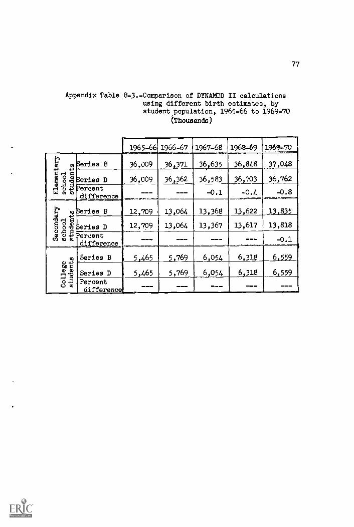
77
Appendix Table B-3.-Comparison of DYNAMO II calculationsusing different birth estimates, bystudent population, 1965-66 to 1969-70
(Thousands)
1965-66 1966-67 1967-68 1968-69 1969-70
04-,
04-,0 H 01 8,8
H 0rii co 0)__Afference
; 3aeries
0 0 00 o rcf.) .z
0 0 4z?ercenta) 0) 02
Series B 36,009 36,371 36,635 36,848 37,048
Series D 36,009 36,362 36,583 36,703 36,762
Percent ___ --- -0.1 -0.4 -0.8
B 12,709 13,064 13,368 13,622 13,835
aeries D 12,709 13,064 13,367 13,617 13,818
difference___
5,465
5,465
__-
5,769
5,769
--_
6,054
6,054
---
6,318
6,318
- --
-0.1
6,559
6,559
_
00 -I-)bD 0,1 i0+,.0 DI
Series B
Series D
Percentdifferenc
--- .--
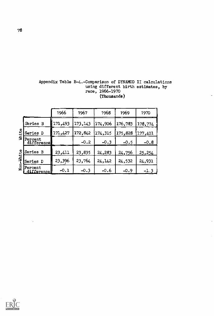
78
0
0z
Appendix Table B-4.-Comparison of DYNAMOD II calculationsusing different birth estimates, byrace, 1966-1970
(Thousands)
1966 1967 1968 1969 1970
Series B 173,143 174,906 176,783 178,774
Series D 1171,427 172,842 174,315 175,828 177,401
Percentdifference -0.2 -0.3 -0.5 -0.8
Series B 23,411 23,835 24,283 24 756 25.254
Series D j23,326 23,764 24,142 24,532 24,931
Percent-0.1 -0.3 -0.6 -0.9 -1,3
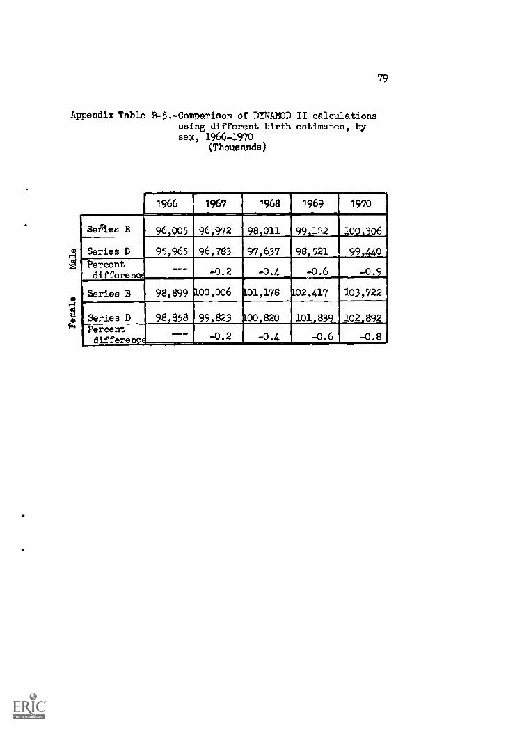
79
Appendix Table 8-S.-Comparison of DYNAMOD II calculationsusing different birth estimates, bysex, 1966-1970
(Thousands)
1966 1967 1968 1969 1970
Series B 96,005 96,972 98,011 99,12 100,306
99,440,
-0.9
Series D 95,965 96,783 97,637
-0.4
98,521
-0.6PercentdifferencE -0.2
Series B 98,899 100;006 101,178 102.417 103,722
Series D 98,858 99,823 00,820 ',101,839 102,892Percentdifference, -0.2 -0.4 -0.6 -0.84
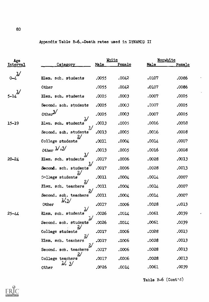
80
Appendix Table B-6.-Death rates used in DYNAMOD II
AgeInterval
WaiteFemale
NonwhiteFemaleCategory Male Male
2/0-4 Elem. sch. students .0055 .0042 .0107 .0086
Other .0055 .0042 .0107 .0086
2/5-14 Elem. sch. students .0005 .0003 .0007 .0005
Second. sch. students .0005 .0003 .0007 .0005
Other2/ .0005 .0003 .0007 .0005
2/15-19 Elem. sch. students .0013 .0005 .0016 .0008
2/Second. sch. students .0013 .0005 .0016 .0008
2/College students .0011 .0004 .0014 .0007
Other 2112/ .0013 .0005 .0016 .0008
2/20-24 Elem. sch. students .0017 .0006 .0028 .0013
2/Second. soh. students .0017 .0006 .0028 .0013
2/0r1iege students .0011 .0004 .0014 .0007
2/Elem. sch. teachers .0011 .0004 .0014 .0007
2/Second. sch. teachers .0011 .0004 .0014 .0007
14/y2/Other .0017 .0006 .0028 .0013
2/25-44 Elem. sch. students .0026 .0014 .0061 .0039
2/Second. sch. students .0026 .0014 .0061 .0039
2/College students .0017 .0006 .0028 .0013
2/Elem. sch. teachers .0017 .0006 .0028 .0013
2/Second. sch. teachers .0017 .0006 .0028 .0013
2/College teachers .0017 .0006 .0028 .0013
24 2/Other .0026 .0014 .0061 .0039
Table B-6 (Conttd)

Table B-6 (Cont'd) 81
AgeInterval Category
WhiteFemale
NonwhiteFemaleMale Male
ai45 & over Elem. sch. teachers .01 .007 .016 .014
3./
Second. sch. teachers .01 .007 .016 .014
2/College teachers .01 .007 .016 .014
2.1Other .0318 .0222 .0352 .0262
V Death Rates based on actual count of deaths for the population,U.S. Department of Health, Education, and Welfare, VitalStatistics of U.S., Vol. II, Mortality, Part A (Table 1-25),1964, Washington, D. C.
zi U.S. Department of Health, Education, and Welfare, "Mortalityby Occupation and Industry" Vital Statistics Special Reports,Vol. 53, No. 2, September 1962 (Female rates estimatedY;
2/ The death rates for the elementary and secondary "dropout" categoryare identical to those of the "other" category for each respectiveage. group.
82
APPENDIX C
Tables of the Effects of Variations inthe Retention Rates of Students and Teachers
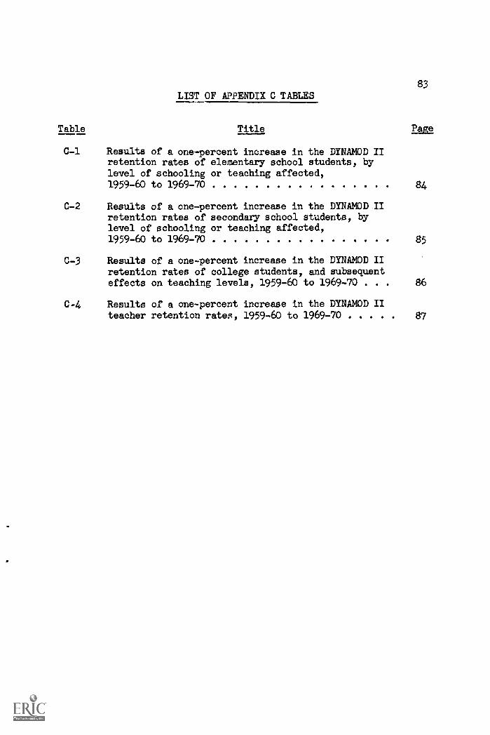
Table
83LIST OF APPENDIX C TABLES
Title Page
C-1 Results of a one-percent increase in the DYNAMOD IIretention rates of elementary school students, bylevel of schooling or teaching affected,1959-60 to 1969-70 84
C-2 Results of a one-percent increase in the DYNAMOD IIretention rates of secondary school students, bylevel of schooling or teaching affected,1959-60 to 1969 -70 85
C-3 Results of a one-percent increase in the DYNAMOD IIretention rates of college students, and subsequenteffects on teaching levels, 1959-60 to 1969-70 . . . 86
C-4 Results of a one-percent increase in the DYNAMOD IIteacher retention rates, 1959-60 to 1969-70 87
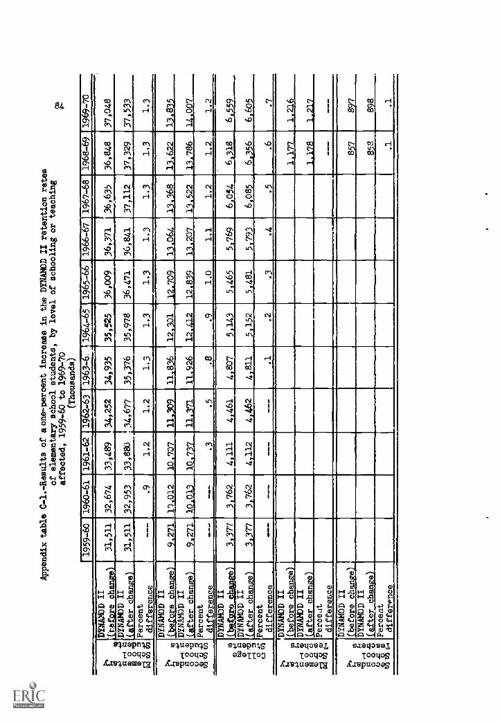
Appendix table 0 -1.- Results of a one - percent increase in the DYNAMOD II retention rates
of elementary school students, by level of schooling or teaching
affected, 1959-60 to 1969-70
(Thousands)
co
1959-60
1960-61
1961-62
1962-63
1963-6
1964-65
1965-66
1966-67
1967-68
1968-69
1969-70
t+'
o.,6
)
A 09
r4 ti)*3
DYNAMOD II
(refore change)
31,511
32,674
33,489
34,252
34,935
35,525
36,009
36,371
36,635
36,848
37,048
DYNAMOD II
(after change)
31,511
32,953
33,880
34,677
35,376
35,978
36,471
36,841
37,112
37,329
37,533
Percent
difference
---
.9
1.2
1.2
1.3
1.3
1.3
1.3
1.3
1.3
1.3
te
93 ..
-1z
g8
913
d3j
°3) to'
DYNAMOD II
(before change)
9,271
1'),
012
10.7
0711
,309
11,$
6]1
368 1
3.522
1.2
13,6
22].
__j,8
25__
13,786
1.2
14.007
1.2
DYNAMOD II
(after change)
9.271
---
10,913
---
10,737 .3
11,371 .5
11,926 .8
12,412 .9
12,839
1.0
13,207
1.1
Percent
difference
(1)
+'
bi) Z CD
ri 'CI
r4 0
o 4-,
DYNAMOD II
before change)
3,377
3,762
4,111
4,461
4,807
5,143
5,465
5,769
6,054
6,318
6,559
DYNAMOD II
(after change)
3,377
3,762
4,112
4,462
4,811
5,152
5,481
5,793
6,085
6,356
6,605
Percent
difference
---
---
---
---
.1
.2
.3
.4
.5
.6
.7
>, k 0
m4-, 0,-4 m$4
11
g 8
a)
.0 0
,--i
00
41`126-1
DYNAMOD II
before change
1 177
1 216
DYNAMOD II
(after change)
1,178
---
1,217
- --
Parceat
difference
tb
,,
b,_
,ti;
08
-50
-0 g
to E.
DYNAMOD II
Sbe fore changal_
857
897
DYNAMOD II
(after chan.te
8 8
:8
Percent
difference
.1
.1

Appendix table C -2. -Results of a one -percent increase in the DYNAMOD II retention rates
of secondary school students, by level of schooling or teaching
affected, 1959-60 to 1969-70
(Thousands)
1959-60
1960-61
1961-62
1962-63
1963-64
1964-65
1965-66
1966-67
1967-68
1968-69
1969-70
a.
.(before
DYNAMOD 11
change)
9,271
10,012
10,707
11,309
11,836
12,301
12,709
13,064
13,368
,13,622
13,835
,t1H
-., g
g 8,kafter
ANPercent
'
DYNAMOD II
change)
9,271
10,070
10,811
11,452
12,012
12,505
12,937
13,312
1'3,633
13,903
14,129
difference
---
.6
1.0
1.3
1.5
1.7
1.8
1.9
2.0
2.1
2.1
,Illefore
0 4'
to g
,$) 43
11 +1
u ril
DYNAMOD II
change)
3,377
3,762
4,111
4,461
4,807
5,143
5,465
5,769
6,054
6,318
6,559
DYNAMOD II
after change)
3,377
3,764
4,123
4,486
4,848
5,202
5,543
5,866
6,170
6,451
6,708
Percent
difference
---
.3
.6
.9
1.1
1.4
1.7
1.9
2.1
2.3
+3
P0 H (1)
ta o a
o .0
01
HO
0)
Wtia
El
DYNAMOD II
(before change)
1,041
1,071
1,104
1,140
1,177.
1,216
1,220
DYNAMO]) II
(after change)
1,042
1,072
1,106
1,142
1,180)
Percent
difference
.1
.1
.2
.2
.3
.3
6211,4 co
g 8 f)
,g, -g g
u3r13
)V
II I
(before change)
745
781
819
857
897
DYNAMO]) II
(after change)
746
783
821
861
901
Percent
difference
I.1
.3
.2
.5
1.4
oa
\-rt
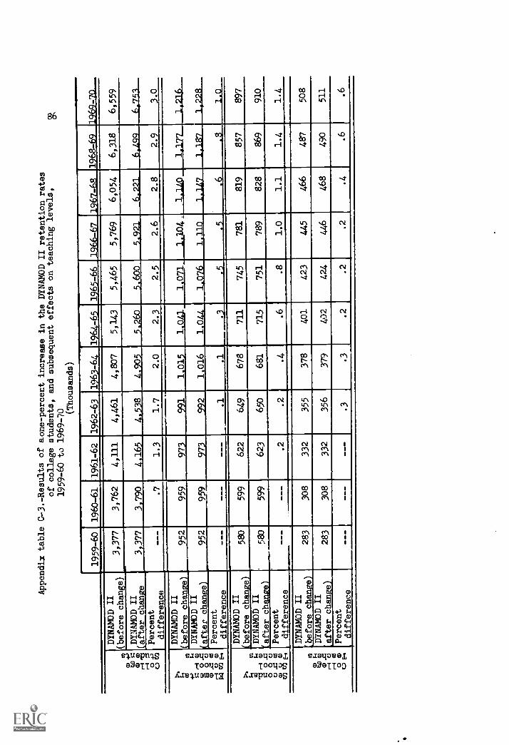
Appendix table C-3.-Results of aone-percent increase in the DYNAMOD II retention rates
of college students, and subsequent effects on teaching levels,
1959-60 to 1969-70 (Thousands)
1959-60
1960-611961-62196-668-6-712-
.
m0
-P,1
,13
.-1 0
0 -P
CO
CO
DYNAMDD II
(before change)
3,377
3,762
4,111
4,461
4,807
5,143
5,465
5,769
6,054
6,318
6,559
DYNAMOD II
(after change
3,377
.---
3,790 .7
4,165
1.3
4.538
1.7
4,905
2.0
5.260
2.3
5.600
2.5
5,921
2.6
6,221
2.8
6,499
2.9
6,759
3.0
Percent
difference
>..
tg
mt,-.1
Ii)
N 8
f,At' g
V)
Es
DYNAMOD II
(before change)
952
959
973
991
1,015
1.016
1,041
1,071
1.104 ,___1V0
1.110
1,147
1.177
1,216
DYNAMOD II
(after changeL
,
952
959
973
992
1,044
1.076
1+187
1,228
Percent
difference
---
---
---
.1
.1
..
.5
.5
.6
.8
1,0
tito k
Yrs r
0.1
00
.0
00
gg
tr) cb E71
DYNAMOD II
before change)
580
599
622
649
678
711
745
781
819
857
897
DYNAMOD II
Nafter change)
r
580
599
623
650
681
715
751
789
828
869
910
Percent
difference
---
---
.2
.2
.4
.6
.8
1.0
1.1
1.4
1.4
0 Po
on w .0
,-, 0
r-I
Cd
o m
0 E
-i
DYNAMOD II
before change)
283
308
332
355
378
401
423
445
466
487
508
DYNAMOD II
after change)
283
308
332
356
379
402
424
446
468
490
511
Percent
difference
---
---
---
.3
.3
.2
.2
.2
.4
.6
.6
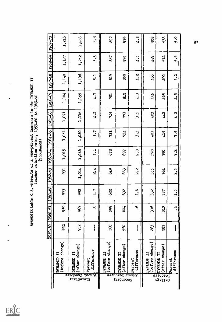
DYNAMOD II
( before change)
DYNAMOD II
(after change)
Percent
difference
DYNAMOD II
ti (before change)
PI 0 t DYNAMOD II
g(after change)
0,4
0 o
ts)
Percent
difference
0 PI
030
H C
)H
0 0 0 E
-1
DYNAMOD II
(before change)
DYNAMOD II
(after change)
Percent
difference
Appendix table 0-4.-Results of a one-percent increase in the DYNAMOD II
teacher retention rates, 1959-60 to 1969-70
(Thousands)
1959-60
1960-61_1961-62
1962-63
1963-64
1964-65-
1965-66
1966-67
1967-68
1968-69
190 -70
952
959
973
991
1,015
1,041
1,071
1,104
1,140
1,177
1,216
952
967
990
1,014
1,046
1,080
1,116
1,155
1,198
1,242
1,286
- --
.8
1.7
2.4
3.1
3.7
4.2
4.7
5.1
r-
5.5
5.8
580
599
622
649
678
711
745
781
819
857
897,
939
580
604
632
663
697
734
771
812
853
895
---
.8
1.6
2.2
2.8
3.3
3.5
4.0
4.2
4.5
4.8
283
308
-
332
355
r
378
401
423
445
466
1-
487
508
283
310
337
364
390
415
440
465
490
514
538
---
.61
1.5
2.5
3.2
3.5
4.0
4.5
5.2
5.5
5.9
88
APPENDIX D
Effects of Variations in theRetention Rates of Students and Teachers
Table
89
LIST OF APPENDIX D TABLES
Title Page
D-1 Comparison of the variations in the student-teacherratio caused by selected increases in student orteacher retention rates, by level of schooling,1959-60 to 1969-70 91
D-2 Effects of setting teacher retention rates equal tosurvival rates while eliminating entries from outsidethe educational system, by level of teaching,1959-60 to 1969-70 92

90
APPENDIX D
Effects of Variations in the Retention Rates of Students and Teachers
The student-teacher ratios discussed in table D-1 that arehypothesized to result from a one-percent increase in the retentionrates of students or teachers contain a minor degree of noncompar-ability with the OE base data from which they are calculated. Thereason for this is that: (a) an elementary school student in DYNA-MOD II is defined as being in grades K through 8, while in OE publi-cations the definition includes only those not attending a junioror senior high school; and (b) IINAMOD II elementary and secondaryschool teachers follow the OE definitions exactly. The number ofgrades 7 and 8 students enrolled in high school organization units(and therefore classified by OE as secondary school students) areabout equal to the equivalent of the total 8th grade enrollment inpublic schools (see OE 10030-66, tables 2 and 3 and OE 10024-65,table 3 plus about 15 percent for nonpublic school enrollments).Thus, about 9-10 percent of the elementary school students affectedby a change in the retention rate in DYNAMOD II would fall in thesecondary school classification of OE. The main effect, therefore,would be concentrated in the third decimal digit of the retentionrate and hence would have only a minor impact on the relative responsepatterns for the students.
Because of this, and also because the teacher classification inDYNAMOD II follows the OE definitions, it was decided to apply thepercent response patterns to one percent changes in the respectivestudent and teacher retention rates from DYNAMOD II to the publishedOE student-teacher ratios for elementary and secondary schools. Thestudent-teacher ratios shown as Series E base data in appendix tableD-1 are combined from the separately published ratios for public andnonpublic schools as shown in OE 10030-66, table 23, using the numberof classroom teachers in table 22 as combinatorial weights. Thestudent-teacher ratios for the college sector were computed directlyfrom the DYNAMOD II calculations.
In table D-2, the teacher retention rates were set to the sur-vival rates (1.0000-death rate), and no entries from outside theeducational system were permitted. By implication, interleveltransfers (e.g., college teachers switching tc secondary school teaching)also were eliminated. No change was made to the flows of collegestudents entering the system.
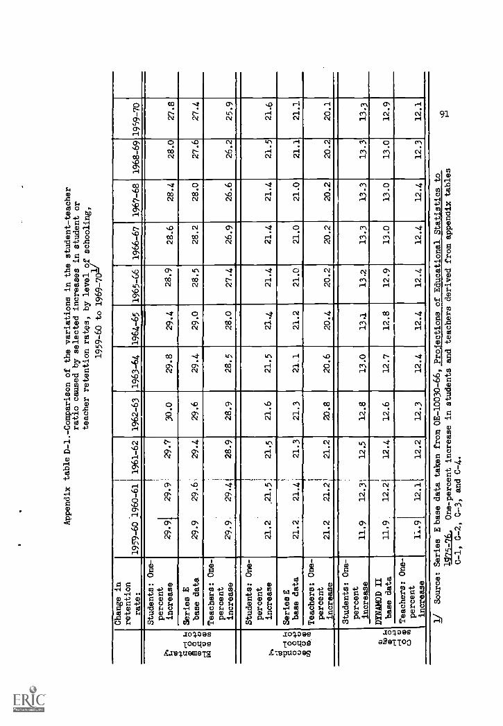
Appendix table D-1.-Comparison of the variations in the student-teacher
ratio caused by selected increases in student or
teacher retention rates, by level of schooling,
1959-60 to 1969-701/
Change in
retention
rate:
i 1
1959-60 1960-611 1961-62
1962-63
1963-64
1964-65
1965-66
1966-67
1967-68
1968-69
1959-70
. Y, 0
so .
0 o
m..m°4-'
0C
)r-
1C
.)11
)
r4 /4
°
Students: One-
percent
increase
29.91
29.9
29.7
30.0
29.8
29.4
28.9
28.6
28.4
28.0
27.8
Series E
base data
29.9
29.6
29.4
29.6
29.4
29.0
28.5-
28.2
28.0
27.6
27.4
Teachers: One-
percent
increase
29.9
29.4(
28.9
28.9
28.5
28.0
27.4
26.9
26.6
26.2
25.9
Pb M Ts
$-.
H o o
0 o -I-
Cl)
2 2
Students: One-
percent
increase
I i
21.2
.21.5!
21.5
21.6
21.5
21.4
21.4
21.4
21.4
21.5
21.6
Series E
base data
21.2.
21.4;
21.3
21.3
21..1
21.2
-
21.0
21.0
21.0
21.1
21.1
Teachers: One-
percent
increase
21.2
21.2!i
21.2
i
20.8
20.6
20.4
20.2
20.2
20.2
20.2
20.1
.
m
os
-1.2
/PI
.13
c..) m
Students: One-
percent
increase
11.9
12.31
12.5
12.8
-
13.0
13.1
13.2
13.3
13.3
13.3
13.3
_
DYNAMOD II
base data
11.9
12.21
12.4
12.6
12.7
12.8
12.9
13.0
13.0
13.0
12.9
Teachers: One-
percent
increase
11.91
12.11
12.2
12.3
12.4
12.4
12.4
12.4
12.4
12.3
12.1
1/
Source: Series E base data taken from 0E-10030-66, Pro ections of Educational Statistics to
1975 -76.
One-percent increase in students and teachers derived from appendix tables
C-1, C-2, C-3, and C-4.
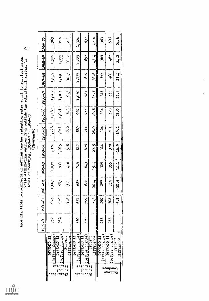
DYNAMOD II
(after change)
DYNAMOD II
:before change)
Percent
M
'00
0 0
00.
0 c
CO
0 0
00-
P
DYNAMOD II
(after change)
DYNAMOD II
before change)
Percent
difference
DYNAMOD II
(after change)
DYNAMOD II
before change)
Percent
difference
Appendix table D-2.- Effects of setting teacher retention rates equal to survival rates
while eliminating entries from outside the educational system, by
level of teaching, 1959-60 to 1969-70
(Thousands)
1959-60
1
1960-61 *1961-62
1962-63
1963-64
II
1964-65 11965-66 11966-67 11967-68
1968-69
1969-70
952
1
974 1
1,003
1,037
1,074
1,116
1,160
1,207
1,257
1,309
1,363
952
959 I
973
j991
1,015
1,041
1,071
1,104
1,140
1,177
1,216
1.6 :
3.1
j4.6
5.8
7.2
8.3
9.3
10.3
11.2
12.1
580
1631 1
687
749
817
889
967
1,050
1,137
1,229
1,324
580
1599
i622
i649
678
711
745
781
819
857
897
I
5.3 ;
10.4
I15.4
20.5
25.0
29.8
34.4
38.8
43.4
47.6
283
290 (
297
305
314
324
334
345
357
369
383
283
308 1
332
355
378
401
423
445
466
487
50C
;
-5.8 1
-10.5
I
-14.1
-16.9
-19.2
-21.0
-22.5
-23.4
-24.2
-24.6
93
APPENDIX E
The DYNAMOD II Computer Program
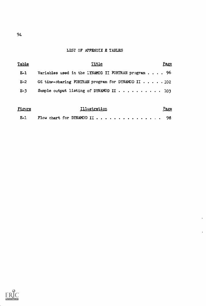
94
LIST OF APPENDIX E TABLES
Table Title Page
E-1 Variables used in the LYNAMOD II FORTRAN program . . . . 96
E-2 GE time-sharing FORTRAN program for DYNAMOD II 102
E-3 Sample output listing of DYNAMOD II 103
Figure Illustration Page
E-1 Flow chart for DYNAMOD II 98
95
APPENDIX E
The DYNAMOD II Computer Program
This appendix consists of four parts: a definition of variables,a flow chart, a FORTRAN program for DYNAMOD II, and a sample outputlisting. The variables in the FORTRAN program are erumerated and adescription of the use of each variable in the program is given intable E-1. An overall flow chart of the model is furnished infigure E-1. /
In considering the FORTRAN program for the model several thingsmust be kept in mind. The program listing shown in table E-2 is onethat has been run and is operational on the GE Time-Sharing System.Features of the GE Time-Sharing FORTRAN are much more general andflexible than versions of FORTRAN for other computer systems. Thiscan be illustrated as follows. First, notice that at the beginningof each line of the program there is a line number. Thus, a FORTRANprogram in GE Time-Sharing FORTRAN consists of enough lines todescribe the program. Consequently, there is no restriction (exceptfor space on a line) as to the 'lumber of FORTRAN statements per line.Each statement is separated by a semicolon. A second feature notusually available in other systems is the accessing of the programlisting in table E-2 is a FILE declaration statement. This affordsthe convenience of storing the sex/race group matrices that make upthe data input to the model in separate files that can be calledwhen needed.
The same program that is listed in this appendix has been run andis made readily available for other systems by putting one FORTRANstatement on each card. The program has been run and tested on aRCA 3301 and an IBM 7094. Listings of these programs along with dataare available on request./
William K. Winters, DYNAMOD II in a Time-Sharing Environment,Technical Note Number 41, Division of Operations Analysis,National Center for Educational Statistics, Office of Education,September, 1967. Note: This reference gives a more detaileddescription of the FORTRAN program for DYNAMOD II.
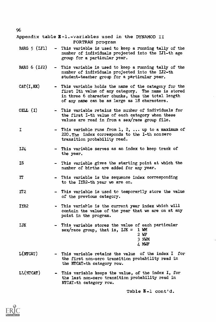
96
Appendix table Z -1.- "variables used in the DYNAMOD IIFORTRAN program
BARG 5 (IJ1) - This variable is used to keep a running tally of thenumber of individuals projected into the IJ1-th agegroup for a particular year.
BARG 6 (IJ2) - This variable is used to keep a running tally of thenumber of individuals projected into the IJ2-thstudent-teacher group for a particular year.
CAT(I,KK) - This variable holds the name of the category for thefirst Ith value of any category. The name is storedin three 6 character chunks, thus the total lengthof any name can be as large as 18 characters.
CELL (I)
I
- This variable retains the number of individuals forthe first I -th value of each category when thesevalues are read in from a sex/race group file.
- This variable runs from 1, 2, ... up to a maximum of220,The index corresponds to the I -th nonzerotransition probability read.
IJ4 - This variable serves as an index to keep track ofthe year.
IS - This variable gives the starting point at which thenumber of births are added for any year.
TT - This variable is the sequence index correspondingto the IYR2-th year we are on.
TT2 - This variable is used to temporarily store the valueof the previous category.
IJK
- This variable is the current year index which willcontain the value of the year that we are on at anypoint in the program.
- This variable stores the value of each particularsex/race group, that is, IJK = 1 WM
2 WF
3 NWM4 MWF
L(NTCAT) - This variable retains the value of the index I for
the first non-zero transition probability read inthe NTCAT-th category row.
LL(NTCAT) - This variable keeps the value, of the index I, forthe last non-zero transition probability read inNTCAT-th category row.
Table E-1 cont d.
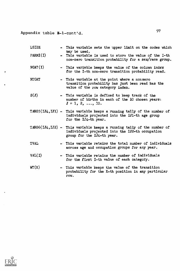
Appendix table E -l- cont'd.97
LSIZE - This variable sets the upper limit on the codes whichmay be used.
PARMI(I) - This variable is used to store the value of the I -thnon-zero transition probability for a sex/race group.
NCAT(I) - This variable keeps the value of the column indexfor the I -th non-zero transition probability read.
NTCAT - This variable at the point where a nonzerotransition probability has just been read has thevalue of the row category index.
S(J) - This variable is defined to keep track of thenumber of births in each of the 10 chosen years:J = 1, 2, ..., 10.
TARG5(IJ4,IJ1) - This variable keeps a running tally of the number ofindividuals projected into the IJ1-th age groupfor the IJ4-th year.
TARG6(IJ4,IJ2) - This variable keeps a running tally of the number ofindividuals projected into the IJ2-th occupationgroup for the IJ4-th year.
TVAL - This variable retains the total number of individualsacross age and occupation groups for any year.
VAL(I) - This variable retains the number of individualsfor the first I-th value of each category.
wr(K) - This variable keeps the value of the transitionprobability for the K-th position in any particularrow.

98
Figure E-1.-Flow chart for DYNAMOD II
Reserve SpaceFor All
SubscriptedVariables
Initialize TheTARG5 (I,J) andTARG6 (I,J) forAll I and J
4Start WithThe FirstSex/RaceGroup, IJK=1
InitializeIndex IJ4To The FirstYear
Define The Year Rangeof Projections
IYR1 = Beginning YearIYR3 = Last Year
ead in Birth Vectorvalues for Each Year
Set MaxSize OnCodes
Initialize L(J)And LL(J) ForEach Possible
Code
Read InCategory Names
And Nonzero Trans-ition ProbabilitiesPlus Their Row and
Column Indices
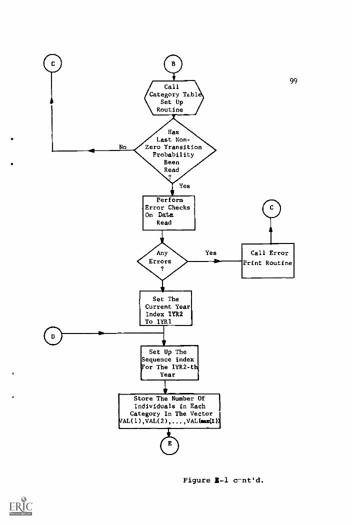
CallCategory Teb1
Set UpRoutine
99
HasLast Non
Zero TransitionProbability
BeenRead9
Yes
PerformError ChecksOn Data
Read
Any
Errors9
Yes Call Error
Print Routine
Set TheCurrent YearIndex 1YR2To IYR1
Set Up TheSequence IndexFor The IYR2-th
Year
Store The Number OfIndividuals in Each
Category In The Vector
iVAL(1),VAL(2),...,VALGaW)
Figure B-1 cant' d.
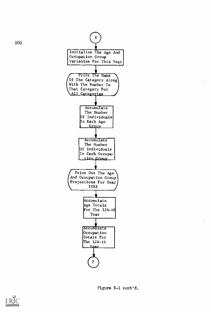
100
Initialize The Age AndOccupation GroupVariables For This Year
Print T e NameiOf The Category AlongWith The Number InThat Category For/All Catego ies
AccumulateThe Number
Of IndividualsIn Each Age
Group
VAccumulateThe Number
Of IndividualsIn Each Occupa-tion(.. oup
Print Out The AgeAnd Occupation GroupProjections For Year
IYR2
AccumulateAge TotalsFor The IJ4-tt
Year
AccumulateOccupationTotals ForThe IJ4-th
Y Ar
Figure E-1 cont'd.
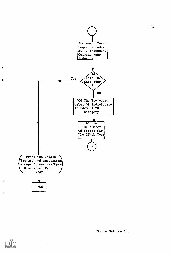
Yes
Increment VearSequence IndexBy 1. IncrementCurrent YearIndex R 1
ForPrint Out Totals
For Age And OccupationGroups Across Sex/RaceGroups For Each
END
Add The ProjectedNumber Of IndividualsTo Each .11-th
Category
Add InThe Number
Of Births ForThe IT-th Yea
Figure E -1 cont'd.
101
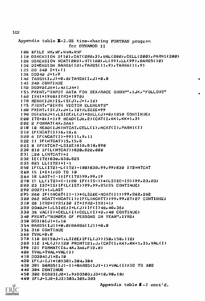
102
Appendix table E-2.GE time-sharing FORTRAN programfor DYNAMOD II
100 SFILE WM,WF,NWM,NWF110 DIMENSION SC10),CAT( 200,3),VAL(200),CELL(200),PARM1(200)120 DIMENSION NCATC200),WTC100),LC99),LL(99),BARG5(10)130 DIMENSION BARG6C10),TARG5C11,9),TARG6C11,9)135 DO 340 1=1,11136 00340 J=1,9140 TARG5CI,J)=0.0;TARG6(I,J)=0.0145 340 CONTINUE150 D0390IJK=1,43IJ4=1155 PRINT,"INPUT DATA FOR SEX/RACE GROUP",IJK,"FOLLOWS"160 IYR1= 1960;IYR3 =1970;170 READ(IJK)IS,CSCJ),J=1,10)175 PRINT,"BIRTH VECTOR ELEMENTS"180 PRINT,CSCJ),J=1,10);LSIEE=99190 001050J=1,LSIEE;LCJ)=0;LLCJ)=0;1050 CONTINUE;200 IT2=0;I=1;9 8EAD( IJK,2)(CAT(I,K14),KK=1,3)202 2 FORMATC4Xs3A6)210 10 READCIJIONICATsCELLCI),NCATCI),PARMI(I)218 IFCNCATCI))6,18,6220 6 IF(NCAT(I)-99)11,9,11222 11 IF(NTCAT)15,15,8223 8 IFCNTCAT-LSIZE)810,810,890230 810 IF(L(NTCAT))820,820,880231 ;20 LCNICAT)=I232 IFCIT2)830,830,825233 825 LLCIT2)=I-1250 IFCLLCIT2)-LCIT2)-100)830,99,99;830 IT2=NTCAT260 15 I=I+1;GO TO 10264 18 LAST=I-1;IFCIT2)99,99,19270 1c: LL(1T2)= I -1 ;20 IFCCIS-1)*(LSIEE-IS))99,23,23;280 23 IST=IS;IFCLCIST))99,99,25;25 CONTINUE;290 00271=1,1-AST295 260 IFCCNCAT( I)-1)*CLSIEE-NCATCI)))99,262,262300 262 NCATT=NCATCI);IFCLCNCATT))99,99,27;27 CONTINUE;310 28 IYR2=IYR1;30 IT= IYR2- IYR1 +1;320 0040J=1*LSI4E;I=LCJ);IFCI)40,40,38;330 38 VACCI)=CELLCI);CELLCI)=0.;40 CONTINUE;340 PRINT,."NUMBER OF PERSONS IN YEAR",IYR2;250 D0310IJI=1,10354 BARG5CIJ1)=0.0;BARG6(IJ1)=0.0356 310 CONTINUE360 TVAL=0.0370 110 00150J=1,LSIZE;IF(L(J))150,150,112;380 112 I=LCJ);120 PRINT121,J,(CAT(I,KK),M=1,3X,VALCI)390 121 FORMAT(I6,4X,3A6,F12.0)400 TVAL=TVAL+VALCI)410 D03041J1=2,10420 IFCJ-1J1*10)301,304,304430 301 BARG5(1J1-1)=BARG5(1,11-1)+VALCI);GO TO 302440 304 CONTINUE450 302 003031J2=1,9J003031j3=10,90,10;460 IF(J-1J27,1J3)303,305,303
Appendix table E -2 cont d.

Appendix table E-2 cont'd. 103
470 305 BARG6CIJ2)=BARG6CIJ2)+VALCI);G0 TO 306480 303 CONTINUE;306 CONTINUE;490 150 CONTINUE500 160 PRINT161,TVAL510 161 FORMATC8H TOTAL =,F12.0)520 PRINT,C8ARG5CIJ1),IJ1=1,9)530 PRINT,CBARG6CIJ2),IJ2=1,9)540 D0341IJ1=1,9;550 341 TARG5( IJ4,IJ1)=TARG5CIJ4,1,11)+BARG5(Ij1)560 D0342IJ2=s,9570 342 TARG6CIJ4,IJ2)=TARG6CIJ4,IJ2)+BARG6CIJ2)580 IJ4=IJ4+1;180 IYR2=IYR2+1;590 IFCIYR2-IYR3)200,200,500 ;200 CONTINUE;600 D0300J=1,LSIZE;IFCLCJ))300,300,215610 215 IT1=LCJ);IT2=LLCJ);TWT=0.;620 220 D0225I=IT1,1T2;K=I-IT1+13630 WTCK)=PARM1CI);TWT=TWT+WTCK);640 225 CONTINUE650 230 D0235I=IT1,IT23K=I-IT1+1;660 J1=NCATCI);J2=LCJ1);670 CELLCJ2)=CELLCJ2)+WTCK)*VALCIT1)/TWT680 235 CONTINUE;300 CONTINUE;690 J=LCIS);CELLCJ)=SCIT)+CELL(J);695 PRINT,"J = "PJ," CELL-CO = ",CELL(J)700 400 GO TO 30705 880 PRINTs"NTCAT = ",NTCAT,"I = ",1," 880"710 GO TO 1571S 890 PRINT,"NTCAT = ",NTCAT, "I = ",I," 890"716 ,G0 TO 15720 99 PRINT,"NTCAT = "rNTCAT,"I = "sIo"CATEGORY IS "725 PRINT,CCAT(I,KK),KK=1,3)."NCATC",I,") = ",NCATCI)730 500 CONTINUE;390 CONTINUE740 PRINT,"TOTALS FOR CODES";750 IJ5=IYR1-1;D0346IJ4=1,11;760 IJ5=IJ5+1;770 PRINT,CTARG5(IJ4,IJ1),IJ1=1,9),IJ5;780 PRINTo(TARG6CIJ4,IJ2),IJ2=1,9);785 346 CONTINUE789 SOPT SIZE790 END DYNAMOD
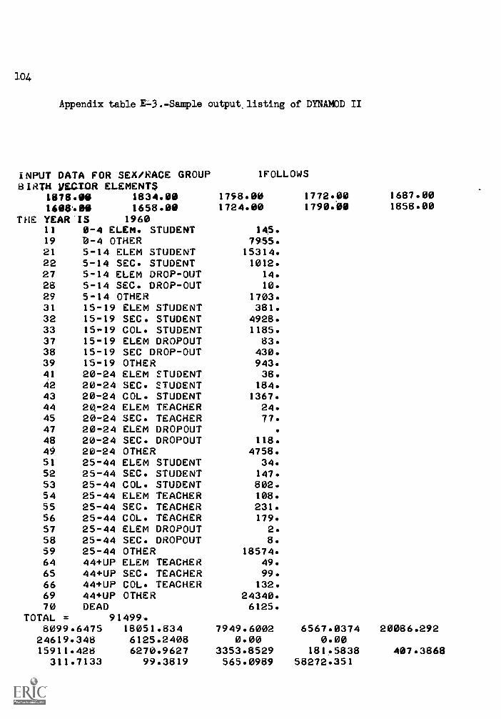
104
Appendix table X.;-3.-Sample output, listing of DYNAMOD II
INPUT DATA FOR SEX/RACE GROUPBIRTH VECTOR ELEMENTS
1070.00 1034.001600400 1658.00
THE YEAR IS 1960
1FOLLOWS
1798.00 1772.001724.00 1790.00
1687.001858.00
11 0 -4 ELEM. STUDENT 145.19 D-4 OTHER 7955.21 5-14 ELEM STUDENT 15314.22 5-14 SEC. STUDENT 1012.27 5-14 ELEM DROP-OUT 14.28 5-14 SEC. DROP-OUT 10.29 5 -14 OTHER 1703.31 15 -19 ELEM STUDENT 381.32 15-19 SEC. STUDENT 4928.33 15,-19 COL. STUDENT 1185.37 15-19 ELEM DROPOUT 83.38 15-19 SEC DROP-OUT 430.39 15-19 OTHER 943.41 20-24 ELEM STUDENT 38.42 20-24 SEC. STUDENT 184.43 20-24 COL. STUDENT 1367.44 20.-24 ELEM TEACHER 24.45 20-24 SEC. TEACHER 77.47 20-24 ELEM DROPOUT48 20-24 SEC. DROPOUT 118.49 20-24 OTHER 4758.51 25-44 ELEM STUDENT 34.52 25-44 SEC. STUDENT 147.53 25-44 COL. STUDENT 802.54 25-44 ELEM TEACHER 108.55 25-44 SEC. TEACHER 231.56 25-44 COL. TEACHER 179.57 25-44 ELEM DROPOUT 2.58 25-44 SEC. DROPOUT 8.59 25-44 OTHER 18574.64 44+UP ELEM TEACHER 49.65 44+UP SEC. TEACHER 99.66 44+UP COL. TEACHER 132.69 44+UP OTHER 24340.70 DEAD 6125.
TOTAL = 91499.8099.6475 18051.834 7949.6002 6567.0374 20086.29224619.348 6125.2408 0.00 0.0015911.428 6270.9627 3353.8529 181.5838 407.3868311.7133 99.3819 565.0989 58272.351
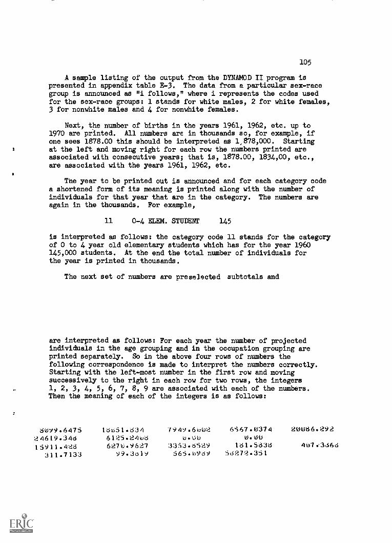
105
A sample listing of the output from the DYNAMOD II program ispresented in appendix table E-3. The data from a particular sex-racegroup is announced as "i follows," where i represents the codes usedfor the sex-race groups: 1 stands for white males, 2 for white females,3 for nonwhite males and 4 for nonwhite females.
Next, the number of births in the years 1961, 1962, etc. up to1970 are printed. All numbers are in thousands so, for example, ifone sees 1878.00 this should be interpreted as 1,878,000. Startingat the left and moving right for each row the numbers printed areassociated with consecutive years; that is, 1878.00, 1834,00, etc.,are associated with the years 1961, 1962, etc.
The year to be printed out is announced and for each category codea shortened form of its meaning is printed along with the number ofindividuals for that year that are in the category. The numbers areagain in the thousands. For example,
11 0-4 ELEM. STUDENT 145
is interpreted as follows: the category code 11 stands for the categoryof 0 to 4 year old elementary students which has for the year 1960145,000 students. At the end the total number of individuals forthe year is printed in thousands.
The next set of numbers are preselected subtotals and
are interpreted as follows: For each year the number of projectedindividuals in the age grouping and in the occupation grouping areprinted separately. So in the above four rows of numbers thefollowing correspondence is made to interpret the numbers correctly.Starting with the left-most number in the first row and movingsuccessively to the right in each row for two rows, the integers1, 2, 3, 4, 5, 6, 7, 8, 9 are associated with each of the numbers.Then the meaning of each of the integers is as follows:
6099.6475 16051.634 /949.6002 6567.0374 20066.29224619.34d 6125.2406 u.00 0.0U
15911.426 6270.9627 3353.6529 161.5636 407:3666
311.7133 99.3619 565.0969 56272.351

106
1 0 - 4 years
2 5 - 14
3 15 - 19
4 20 - 24
5 25 - 44
6 44+
7 Dead
For the example above the number of 0-4 year olds is 8,099,648. The
number 44 years old and older is 24,619,348.
Next, in the third and fourth rows we can associate the integers
1, 2, 3, 4, 5, 6, 7, 8, 9 with each of the following categories:
1 Elementary school student2 Secondary school student
3 College teacher
4 Elementary school teacher
5 Secondary school teacher
6 College teacher7 Elementary school dropout
Secondary school dropout
9 Other
After the data for the individual sex-race groups (including their
respective subtotals) have been obtained, provisions are available for
taking subtotals, by year, over all four sex-race groups. The format
is the same as for the subtotals for the individual groups shown above.
107APPENDIX F
METHODOLOGY OF PARAMETER ESTIMATION INDYNAMOD II: AI ANNOTATED BIBLIOGRAPHY
The list of technical notes presented below discuss in depth theparametric estimating procedures and data sources used in the develop-ment of DYNAMOD II. The abstractor's names appear in parentheses atthe end of the abstract.
Technical Notes are working papers of the Division of OperationsAnalysis, and as such they do not new,ssarily reflect the officialpolicy of the U. S. Office of Education. They have been circulated tothe educational community by means of deposit in the Educational Re-sources Informatio Center. The Educat4onal Resources InformationCenter (ERIC), is a national information system designed to serve theeducational research community by making available to any user currel::.educational research and research-related material. ERIC is based onthe network of 18 information clearing houses or documentation centerslocated throughout the country and correlated through ERIC Central inWashington, D. C. Research reports available through the ERIC systemare listed in the monthly abstract journal Research in Education. Eachmonthly issue includes abstracts and detailed indices of cited researchdocuments and accumulative indices will be published semiannually. Theannual subscription price is $11, single 13sues $1. Additional inquiriesto Superintendent of Documents, U. S. Government Printing Office,Washington, D. C. 20402. Documents are made available either in hardcopy or microfiche from the ERIC Document Reproduction Service (EIBS),Bell and Howell Company, 1700 Shaw Avenue, Cleveland, Ohio 44120. Forfurther information on the ERIC information network and its service,write to Educational Resources Information Center, U. S. Office ofEducation, 400 Maryland Avenue, S. W., Washington, D. C. 20202.
Single copies of particular Technical Notes abstracted herein maymay be obtained by writing directly to: Division of Operations Analysis,National Center for Educational Statistics, U. S. Office of Education,400 Maryland Avenue, S. W., Washington, D. C. 20202.

108
Birth and Death Inputs
TN-11 BIRTH AND DEATH PROJECTIONS USED IN STUDENT-TEACHERPOPULATION GROWTH MODELS. Tetsuo Okada, November 14, 1966
This note presents a brief description of the methodology used toproject births and deaths in DYNAMOD II (See TN-34). For death rates,the most recently available data (1964) by sex and race was used andassumed to be constant over the period of projection. For projectednumber of births, Grabill's marriage-parity-progression method wasemployed. This method takes account of the variables of marriage,parity (number of previous children born), and birth interval (timebetween marriage and successive children). (T. Okada)
First-Stagg Trial Estimates
TN-28 DROPOUT AND RETENTION RATE METHODOLOGY USED TO ESTIMATEFIRST-STAGE ELEMENTS FOR DYNAMOD II. Edward K. Zabrowskiand John T. Hudman, April 20, 1967
DYNAMOD II is a computerized Markov-type demographic model of thetime flows of the educational population (See TN-34). The model wasbuilt in two stages: in the first stage, the population was divided intomale and female, and the transition probabilities for thu respectiveeducational groups were estimated. In the second stage, these prob-abilities were factored further to develop sex-race-age-educationalcategory parameters. This note concentrates primarily on the proceduresused in estimating the male/female flow parameters (transition prob-abilities) for elementary, secondary, and college students. Estimatingformulas and data sources are given. An appendix is devoted to secondaryschool students' dropout rates. The estimating procedures used for theremaining transition probabilities is discussed in TN-24 and TN 39.(E. Zabrowski)
TN-39 METHODOLOGY USED TO ESTIMATE FIRST-STAGE ELEMENTS OF THETRANSITION PROBABILITY MATRICES FOR DYNAMOD II: TEACHERSAND EXTRA-SYSTEMS FLOWS. Edward K. Zabrowski,September 18, 1967
This note is essentially a continuation of the exposition of thetransition probability estimation procedures first discussed inTechnical Note Number 28. The procedures developed describe how esti-mates were obtained of the chances that a person in a given educationalcategory in one year (e.g., male college students) will move to an-other educational category by the next year (e.g., male elementaryschool teachers). Specifically discussed in the development of theprobabilities that collage students will enter elementary, secondary
109
or college teaching; that a teacher in one level in a given year willtransfer to another level of the next year (e.g., that college teacherswill transfer to secondary school teaching); and that persons outsidethe educational system will enter one of the pre-defined educationallevels: elementary, secondary or college students and elementary,secondary or college teaching. All estimates were developed from variousdocumented sources. (E. Zabrowski)
Final Stage Trial Estimates
TN-12 ESTIMATION OF AGE TRANSITION PROBABILITIES. Judith R. Zinter,December 8, 1966
This note describes the procedure followed in estimating agetransitions for DYNAMOD II, a computerized Markov chain modelcharacterizing the flow of students and teachers through the educationalsystem over time (See TN-34). The age transitions are presented in theform of probability matrices, one for each sex-race group. By means ofthese matrices, one can find the probability that an individual will(1) remain in a given age group, (2) move into the next age group, or(3) die. The age groups for which transition probabilities are estimatedare 0-4, 5-14, 20-24, 25-44 years old, and 44 years old and over.(J. Zinter)
TN-40 ESTIMATION OF SECOND-STAGE DROPOUT RATES FOR STUDENT-TEACHER POPULATION GROWTH MODEL (DYNAMOD II).Judith R. Zinter, August 28, ]967
This note presents the methodology used to estimate dropout ratesfor DYNAMOD II, a computerized Markov chain model of student and teacherflows over time (See TN-34). Dropout rates are estimated for elementaryand secondary students by race and sex for the following age groups:less than 15, 15-19, 20-24, and 25-44 years of age. (J. Zinter)
TN-42 TRANSITION PROEPHILITIES FOR STUDENT -TEACHEP POPULATIONGROWTH moral, (D/NAMOD II). Judith R. Zinter, September 18,1967
This note lists the transition probabilities in use in DYNAMOD IIas of the date the note was published. These transition probabilitiesare estimates of the chance that an individual in a given sex-race-age-educational level category in one year will move to another feasiblecategory b: the following year. (J. Zinter)

110
Computing Methodology
TN-45 DYNAMOD II IN A TIME-SHARING ENVIRONMENT. William K. Winters,October 23, 1967
This Lote describes in detail the development of the FORTRAN computerprogram for the Student-Teacher Population Growth Model (DYNAMOD II), amodel of the flows of students and teachers over time. (See TN-34).The program is written for use on the GE-235 Time-Sharing System. Flowcharts of the source program and definitions of the program variablesare included in the note as well as complete listings of the sourceprogram and data files and sample listings of output. (J. Zinter)
*U. S. GOVERNMENT PRINTING OFFICE 1988 0 - 307 -520