Students Today, Teachers Tomorrow? The Rise of Affordable

Private Schools

Tahir Andrabi (Pomona College) Jishnu Das (World Bank)

Asim Ijaz Khwaja (Harvard University)∗

February 2006

Abstract

This paper assesses the constraints on the emergence of private schools, a sector thatincreasingly accounts for a large share of primary enrollment in low-income countries. Weuse data from Pakistan, where 35 percent of children at the primary level are in mainstreamprivate schools. We highlight the critical role of the public sector in determining privateschool existence: Instrumental variable estimates indicate that private schools are fourtimes as likely to locate in villages with a girls’ high school compared to those without, anincrease of 29 to 35 percentage points. In contrast, there is little or no relationship betweenprivate school existence and pre-existing girls’ primary or boys’ primary and high schools.The data support a supply-side explanation: in an environment with low female mobilitydue to cultural restrictions, women receive significantly lower wages in the labor market.Private schools therefore locate in villages with a greater supply of local high-school educatedwomen. Indeed, the private school wage-bill is 20 percent lower in villages with pre-existinggirls’ high schools. These findings bring together three related concepts to explain whereprivate schools arise–the inter-generational impact of public schools, the role of culturallabor market restrictions, and the prominent role of women as teachers. They also suggestthe continuing importance of the government sector in creating the cohort of women withsecondary school education who can then become the teachers in private schools.

∗Pomona College, Deverlopment Research group, World Bank, and Kennedy School of Government, HarvardUniversity. Email: tandrabi@pomona.edu; jdas1@worldbank.org; akhwaja@ksg.harvard.edu. This paper wasfunded through grants from the PSIA and KCP trust-funds and the South Asia Human Development Groupat the World Bank. We thank Hanan Jacoby, Ghazala Mansuri, Sendhil Mullianathan and Tara Vishwanathfor long discussions and seminar participants at Lahore University of Management Sciences, Harvard University,The World Bank, Wharton, IUPUI, University of Michigan and University of Maryland for comments. We arespecially grateful to Tristan Zajonc for exceptional research assistance. Assistance from the Project Monitoringand Implementation Unit in Lahore is also acknowledged. All errors are our own. The findings, interpretations,and conclusions expressed in this paper are entirely those of the authors. They do not necessarily represent theview of the World Bank, its Executive Directors, or the countries they represent.

1

I Introduction

There is a quiet educational revolution going on in the South Asian countryside. While low-

income countries around the world struggle with getting teachers to rural areas, the private

sector has made significant progress. In South Asia, India, Bangladesh and Pakistan all report

high and increasing shares of private schooling in primary education with shares of 15, 38 and

35 percent respectively. In Pakistan–the focus of this study–8000 new private schools were

set up in 1999, almost half in rural areas.1 We study the location decisions of private schools

and examine an important constraint on the widespread use of private schooling. We show that

private schools are four times as likely to locate in villages with girl’s high schools compared to

those without. These results point to a supply-side channel: Girl’s public high schools create

the next generation of teachers to staff private schools.

Recent empirical research makes a strong case for the private sector in education. Expand-

ing school choice leads to better overall educational performance. This is due to both the direct

effects of better performance in private schools (Jimenez and others 1999, Tooley and Dixon

2006, Figlio and Stone 1997) as well as improvements in public schools from increased compe-

tition and greater per-child resources in the government sector (Hoxby 1994). In low-income

countries, greater private schooling also has significant fiscal implications–the unionization and

pay-grade of public teachers implies that per-child costs of private schools is half that of their

public counterparts (Jiminez and others 1999, Kip and others 1999, Orazem 2000, Hoxby and

Leigh 2004).

In addition, in countries such as Pakistan one of the largest determinants of school enroll-

ment is distance, and the adverse effect of greater distance to school is larger for girls compared

to boys (Alderman and others 2001, Jacoby and Mansuri 2006, Holmes 1999, Andrabi and

others 2006). Private schools decrease the average distance to school, thus increasing overall

enrollment. Kip and others (1999) provide strong evidence for this hypothesis by examining

a randomly allocated subsidy for the creation of private schools in rural Pakistan. They find

that the subsidy led to increases of 14.6 and 22.1 percentage points in female enrollment for1These schools are not religious schools or madrassas. The vast majority are co-educational, English medium

schools that offer secular education. Contrary to popular views, religious schools play a small role in Pakistan,comprising less than a one percent share and an even lower share in settlements with a private school (Andrabiand others 2006a).

2

two of three program districts (Kip and others 1999 and Orazem 2000). There is thus a per-

suasive argument for separating the financing of education from the provision of education,

perhaps through instruments such as school vouchers. Larger differences in learning outcomes

and teacher’s wages between the public and private sector in low-income countries compared

(say) to the US, indicate that the impact of such programs may be magnified.

Key to the question of whether private schools can become a vehicle for mass education is un-

derstanding whether such schools arise where public schools are poor or non-existent. Although

close to 7 million children in Pakistan–one of every three enrolled–are in private primary

schools (Federal Bureau of Statistics, 2001), there is considerable geographical variation–27

of 102 districts report less than 5 percent of enrolled children in private schools; in contrast,

another 27 districts report private enrollment shares exceeding 25 percent. Exploiting this vari-

ation provides insights into the working and limits of the private sector. We focus on a specific

question – what determines where private schools arise?2

Our results highlight the critical role of the public secondary sector, of women, and of

supply-side factors. We identify a large positive effect of pre-existing girls’ public high schools

(schools that offer classes from Grades 6 to 12 in addition to primary) on the decision to open a

private school. We argue that this effect arises because of geographically limited labor markets

for educated women. Private schools are able to operate widely and profitably despite charging

low fees, by taking advantage of a low-cost teaching resource – locally educated women willing

to work at low wages due to restricted mobility and hence labor market opportunities. Since

all public schooling is gender segregated with different schools for boys and girls, the pool of

locally educated women depends critically on the availability of a girls’ secondary school in the

village.3

The initial conditions for the increase in private schooling in Pakistan were thus laid during

2We focus on the existence of private schools rather than their enrollment share for two reasons. Most variationin the number of children enrolled in private schools is driven by the extensive (that is, whether or not there isa private school in the village) rather than the intensive (variation in private school enrollment conditional onexistence) margin. Thus, it is of independent interest to study the existence of such schools. An option wouldbe to look at the share of private schooling in total enrollment. The only data that permits us to construct thisvariable is based on household surveys. Unfortunately, as we discuss below, samples in such surveys are too smallfor us to examine the main hypothesis presented here.

3 In some cases, girls are allowed to attend boys’ schools in the village if there are no girls’ school, but only atthe primary level. At the secondary level, there is strict segregation.

3

the 1980s, with a systematic policy of public high school expansion for girls. Private schools

were more likely to locate in villages that received a girl’s high school during this period of school

expansion; similar results do not extend to girl’s primary schools or boy’s schools (primary or

high). The numbers are striking: among villages that did not have any girl’s school in 1981,

by 2001 there were private schools in only 11.5 percent of those that still did not have a girl’s

school, 12.5 in those that received a girl’s primary school and 30.8 in those that received a

girl’s high school.

This positive association between private schools and girl’s high schools could reflect non-

random placement patterns. If girl’s high schools were constructed in villages with high ag-

gregate demand for education, estimates reflect differences in demand rather than the causal

impact of girl’s high schools on private schooling. Similarly, if they were built in villages with

systematically lower wages, a positive correlation could reflect aggregate differences in labor

market conditions whereby teacher salaries in private schools were lower than in random vil-

lages.

We address non-random selection in a number of ways. We match village-level data from

1981 and 1998 and show that apart from village population, there were no significant baseline

differences in village-level characteristics for villages that did and did not receive a girl’s high

school. These data also allow us to remove unobserved time-invariant characteristics through a

first-difference specification. However, these methods do not address the issue that the place-

ment of girl’s high schools could be correlated with time-varying village characteristics.

Our preferred specification addresses concerns arising from time-varying omitted variables

through an instrumental variables approach. The identification problem arises from a rela-

tionship between village population and the placement of girl’s high schools combined with a

similar relationship between village population and the placement of a private school. Within

this context, one option is to base identification on nonlinearity and discontinuities in the func-

tion relating the setting up of girl’s high schools and village population (Fisher 1976). If these

nonlinearities can be justified and understood on the basis of an existing policy, we can iden-

tify the causal relationship between girl’s high schools and the setting up of private schools by

simultaneously controlling for the independent effects of village population.

4

We use the stipulated policy framework for the placement of girl’s high schools to construct

such an eligibility rule. Government rules specified a number of conditions to determine whether

a village was eligible, which we argue can be modelled as a "minimum population condition"

and a "population rank condition". In particular, villages satisfy an eligibility condition if

(a) their population was above a certain threshold (500 inhabitants) and (b) their population

was the largest within a geographically contiguous administrative unit of 3-4 villages, called a

patwar-circle.

Together, these conditions generate an eligibility variable that is highly correlated with

the actual placement of a girl’s high school–villages in the eligible group were 60 percent

more likely to receive a girl’s high school compared to those that were not. Moreover, non-

linearities in the eligibility requirement (two villages with same population may be eligible or

not depending on their population rank within the administrative unit) allow us to control for

linear (and polynomial) effects of village and neighboring villages’ populations that might have

independent effects on private school placement. Under the assumption that private school

placement is not determined in the same non-linear fashion as the eligibility requirements, the

estimated instrumental variables coefficient is consistent and unbiased.

From a base estimate of 10 percentage points increase (75 percent) in the cross-sectional

data, the impact of girl’s high schools on the existence of a private school increases to 15

percentage points once we control for time-invariant village-level characteristics and to 35 per-

centage points with the instrumental variables specification. We discuss the properties and

robustness of this instrument to various samples and construct falsification tests to show that

the instrument is unrelated to the setting up of private schools in areas where girl’s high schools

were not constructed. The consistent increase in the coefficient as we control for unobservable

characteristics suggests that girl’s high schools were placed in areas with systematically lower

demand for education. We postpone a discussion of why this may be so till later.

What are the channels through which girl’s high schools lead to an increase in the likelihood

of private school existence in the village? In the words of a local entrepreneur:

“The big problem”, he said,“is teachers. In most villages, I can set up a private school, but

who will teach? All the men are working and if I pay them what they want, I will never make a

5

profit. I cannot get women from other villages–who will provide the transport for them if it gets

dark? How will she be able to work in another village if she is married? The only way we can

work is if there are girls who can teach in the village–that is why, I ask if there is an educated

girl who can teach. I can pay them Rs.800 ($14) a month and run the school. Otherwise it is

not possible.”

Taken at face-value, our entrepreneur’s travails suggest that one channel through which

girl’s high schools led to the expansion of private schools was by creating teachers. Of course,

this need not be the only one–educated women also play an important role in stimulating

demand both for their own children and those around them. In addition, girl’s high schools

could also increase awareness or change preferences towards education in the village and these

may be different from what girl’s primary or boy’s schools can do.

Nevertheless, the entrepreneur’s suggested hypothesis is not easily dismissed. In 1981, there

were 5 literate women in the median village in Punjab–the largest and most dynamic province

in the country. High-school education was a rarity: 60 percent of villages in the province had

3 or less such women and 34 percent had none. While hiring men is clearly an option, data

on private school teachers show that this would not come cheap–wage differentials between

men and women controlling for education, age and experience suggest a 20-25 percent discount

for female teachers. In addition since private schools are all coeducational, the presence of

female teachers could be instrumental in getting more girls into school. Interestingly, an (early)

innovative randomized experiment that tried to set up private schools in rural areas failed

precisely because teachers could not be found (Alderman 2003).

In an independent survey, we do indeed find that most private school teachers are females

who were educated in the same village as the one they are teaching in (Andrabi and others

2005b). With few employment opportunities outside teaching (both due to the lack of options

and social constraints on what women can and cannot do), private entrepreneurs could take

advantage of the locally available and constrained pool of educated women in the villages where

they set up; conversely they would be severely limited if they tried to locate in villages without

high school educated women.

Our results support the “women-as-teachers” channel. We show that private school existence

6

is affected only by pre-existing girls’ high schools–girls’ primary or boys’ high/primary schools

have little or no effect. For a demand-side explanation one would have to assume that educated

women stimulate demand for education in the village much more than equally educated men or

women/men with lesser (primary) education. More directly, our results show that not only do

pre-existing girls’ high schools more than double the fraction of highly educated local women,

but that private schools are more likely to exist when there are more high-school educated

women in the village, whereas similarly educated village men have no effect.

These predictions are on the “quantity” margin and more nuanced demand based channels

could also explain the observed location patterns of private schools. A more compelling test is

on the price/wage-bill margin. If the supply-side channel is more important, the wage-bill of a

private school should be lower in villages with pre-existing public girls’ high schools–demand

based explanations suggest the opposite. Indeed, the wage bill is 20 percent lower in villages

with a girls’ high school; interestingly, this is also the difference in male and female teacher’s

wages using individual wage-level data and controlling for educational qualifications, age and

school fixed-effects.

This paper adds to the literature on the location decisions of private schools. In the US

there is some evidence that the religious affiliation of communities and the quality of public

schools are important (Hoxby 1994, Downes and Greenstein 1996); a recent paper from India

confirms a correlation between private and public school location across communities (Tilak

and Sudarshan 2001). To our knowledge this is the first paper that establishes a causal cross-

generational link between public high schools and the location of private schools. While in

a static framework public schools may deter private school entry, in a dynamic setting, the

supply-side effects of producing educated teachers in public schools are positive and large.

The paper is structured as follows: Section II is a guide to the educational background and

institutions in Pakistan. Section III presents some patterns that illustrate our main findings.

Section IV discusses the data and Section V details our methodology. Sections VI presents the

results. Section VII concludes.

7

II Background and Institutions

Pakistan has a population of 132 million people living in four main provinces–Punjab, Sindh,

North Western Frontier Province and Balochistan. They, along with Islamabad the federal

capital, comprise about 97 percent of the country’s population. Punjab, the focus of our study,

is the largest province with 56 percent of the population, a majority of whom are in rural areas.

Education provision is managed by provincial governments but there are recent changes at the

local government level that aim to devolve such provision to the lowest tier.

Both the literacy rate and primary school enrollments are low, even compared to countries

in Pakistan’s own income range and to others in South Asia. Pakistan’s adult literacy rate of

43 percent compares to 54 percent for the South Asia average. The gender gap in educational

enrollment is large as are differences between rural and urban areas and the rich and poor. The

gross enrollment rate for the top expenditure decile is twice as high as that for the lowest decile.

Given these conditions, increasing the stock of human capital is clearly a priority, especially for

the poor, and especially for girls.

The extent to which supply-side interventions, such as the construction of schools, can help

in increasing human capital is constrained by the nature of the labor market. While returns

to education in Pakistan appear to be fairly high at 15.2 percent (Psacharopolous 2002) and

higher for women compared to men (World Bank 2005), labor force participation for women is

low. Labor force participation was less than 5 percent for women in rural areas according to

a household survey fielded in 2001 (Pakistan Integrated Household Survey, 2001) and of those

employed in paid jobs, XX percent were working as teachers. Moreover, wages for women were

30 percent lower than for men after controlling for educational qualifications and experience

(World Bank 2005). Low mobility for women appears to play a role–a recent study documents

that safety concerns and a strong patriachal society restrict the ability of women to find work

outside the village they live in (World Bank 2005).

The government’s position on the role of private schools has oscillated during the last 30

years. Private Schools were nationalized in 1972 amidst a mass government program of nation-

alization of all industry, but in 1979 the policy was reversed. Private schools were allowed to

open, and schools taken over by the government were gradually returned to the original owners.

8

However, there was no systematic policy towards such schools or any subsidy in the form of

grants (to parents or directly to schools) unlike in India or Bangladesh (where there are a large

number of private aided schools–the Indian equivalent to the Pakistani private schools are the

private unaided schools). Prior to nationalization, private schools catered primarily to a niche

market, restricted to large cities. The market was dominated by missionary run private schools

(or local schools imitating the missionary model), mainly used by the elite.

Within this milieu, the government in consort with international donors tried to increase

investment in human capital through a series of "Social Action Programs" or SAPs. The SAP

initiated in 1980 called for large investments in the provision of education. School construction

was a large part of the education component, and specific guidelines were set for villages where

schools should (and should not) be built.

Figure I shows that this program had an effect, at least on school construction. The figure

plots the number of years a school has existed for all villages in Punjab and for four types of

schools–primary and high for boys and girls. The kernel density shows a substantial increase

in construction around the years of the SAP III program; in the case of girls, this is the largest

construction period since 1930. While most girl’s high schools were built between 1960 and

1965, there is again a definite hump around the SAP III years; in the case of boy’s high schools,

there is no such increase–most such schools appear to have been around since 1930.

A. What do private schools in rural Pakistan look like?

As part of a study on Learning and Educational Achievement in Punjab Schools (LEAPS), we

are working in 112 villages, selected randomly in 3 districts of Punjab from a list of villages

with at least one private school in 2000–this guarantees significant choice for all households in

our sample, and allows us to compare public and private schools within the same geographical

area. In these villages, we followed a matched sample of 12000 children, 5000 teachers, 800

schools and 2000 households over three years. Several findings from the first year of the study,

summarized in Table 1, are relevant for the current paper (all findings are drawn from Andrabi

and others 2006b and Andrabi and others 2006c).

First, private schools are affordable. The median fee of a rural private school in Pakistan is

Rs.1000 ($18) per year, which represents 4 percent of the GDP per capita. In contrast, private

9

schools (elementary and secondary) in the US charged $3524 in 1991. At 14 percent of GDP

per capita, the relative cost of private schooling is almost 3.5 times as high in the US compared

to Pakistan. Perhaps as a result of their affordability, private schools are increasingly accessed

by even those from the lowest income decile.

Villages with private schools perform significantly better on a number of traditional educa-

tional outcomes (Table 1, Panel A). Overall enrollment is significantly higher (61 percent vs. 46

percent), as is female enrollment (56 percent vs. 35 percent). In villages with private schools,

17 percent of the households in the poorest tercile are enrolled in private schools and this is

virtually the same as private school enrollment among the rich in villages without such schools

(18 percent).

Second, private schools, while offering comparable if not better facilities (classrooms per-

student, black-boards and seating arrangements), incur half as much expenditures per child

compared to public schools–Rs. 1,012 per child for the median private school compared to

Rs. 2,039 for the median public one. These differences remain as large after controlling for

parental/village wealth and education.

Given that teaching costs form the bulk of schooling costs (just under 90 percent in private

schools), these savings stem primarily from lower teacher salaries in the private sector. Wage

comparisons of teachers in the private and public sector show that private school wages are

20 percent those of teachers in public schools (Table 1, Panel B). In addition, there is a large

and significant discount for female teachers in the private sector (but not in the public sector).

These differences remain large and significant after controlling for location (village fixed-effects),

training and education. With school fixed-effects and controls for education, training, experi-

ence and residence we estimate that private school male teachers earn 21 percent more than

females.

Third, children’s test-scores are higher in private schools. In tests administered by our team

to students finishing class 3 through the LEAPS study, private schools students outperform

public school students (Table 1, Panel C). The differences are large with private school stu-

dents typically scoring 0.9 standard deviations higher in English, and 0.39 standard deviations

higher in Mathematics. While selection into private schools could explain part of the difference,

10

interestingly there is only a small change in the private-public schooling gap after controlling

for child, household, and village attributes. The difference for English drops to 0.85 standard

deviations and that for Mathematics to 0.34 standard deviations.

As is well known, establishing causality for each these findings is an empirically difficult

task. Nevertheless, the size of the differences in raw comparisons and with additional covariates

presents strong prima facie evidence that the benefits of private schools discussed above are

very evident in the rural Pakistani case.

III Some Illustrative Patterns

Three figures outline the basic patterns of interest for this paper. Figure II shows the date of

construction for every private school based on a census of private schools in 2001. A quarter of

the private schools in 2000 were built in the previous year, and there is an exponential decline as

we move further back in time. During the early half of the nineties, most schools were in urban

areas. However, there was a shift around 1995 with an increase in the share of rural villages.

This pattern continues till 2000 (the last year for which we have data) when approximately half

of all schools were set up in rural areas.4

Figure III shows the relationship between the existence of a private school and various types

of government schools. We regress the existence of a private school on the number of years that

the village has had a primary or high school (both boys and girls) using a probit specification.

The figure plots the predicted probability of a private school against exposure to a public school;

these probabilities are then to be understood as the marginal effect of exposure to each type of

public school, controlling for other public schools in the village.

Boy’s primary schools appear to do nothing with an almost flat relationship over the 20-year

horizon. Girl’s primary schools and boy’s high schools do marginally better and the regression

implies a 2-3 percentage point increase in the probability of a private school with 10 years of

exposure. The role of girl’s high schools stands out. There is a private school in one-fifth of

4Although these data confound school construction and survival, comparisons with the number of schoolsreported in a 1985 study (Jimenez and Tan 1985) suggest that most of the increase is real. Correcting for thesurvival rate (around 5 percent of all schools die every year) still implies a phenomenal growth rate during thenineties.

11

all villages with a girl’s high school, or a 7-8 percentage point increase for every additional 10

years of exposure. The marginal impact of a girl’s high school on private school existence is

large and significant.

Figure IV is another cut at the data showing the predicted relationship between private

school existence and the percentage of men and women with high school education (8 or more

years of schooling) in every village. Increasing the percentage of women with high school ed-

ucation in a village increases the probability of a private school from 10 percent (0 percent

educated) to almost 100 percent (100 percent educated). Educated males again play an atten-

uated role–at the mean of the sample for female literacy, increasing high school males from 0

to 100 percent increases the probability of private school existence from 7 to 32 percent.

Both these figures suggest that women matter–girls’ high schools (henceforth GHS) have

a qualitatively different role in the setting up of private schools as do educated women in the

village. In addition, labor market conditions may be important. As we saw above, female

teachers are significantly cheaper, and the available pool of female teachers could drive the

location decisions of private schools.

IV Data

To examine whether these correlations are causal, we employ four data sources: (a) a complete

census of private schools; (b) administrative data on the location and date of construction of

public schools and (c) data on village-level demographics and educational profiles from the

2001 and 1981 population censuses. The Federal Bureau of Statistics undertook a census of

all private schools in 2001 and data on public school construction is available from provincial

Educational Management Information Systems (EMIS). Further, population censuses carried

out in 2001 and 1981 (two years after the denationalization of private schools) provide both

contemporaneous and baseline data on village-level characteristics.

An important step was matching these data at the village level. Given the high level of

data fragmentation (these data are collected by different institutions without a common coding

scheme) and variations in the spellings for village names some choices had to be made. By

relying on phonetic matching algorithms and a manual post-match, we matched the public

12

school (EMIS) data to both the 1981 and 2001 censuses. Given the availability and nature

of the data, we study the province of Punjab and only for rural areas. Our matched sample

consists of 18,119 villages out of 25,941 in 2001 in Punjab province with a population of 42.3

million in 1998, representing 84 percent of the total rural population of the province.

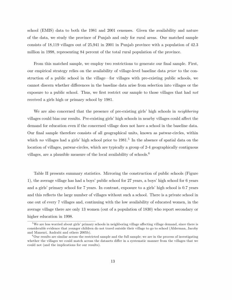
From this matched sample, we employ two restrictions to generate our final sample. First,

our empirical strategy relies on the availability of village-level baseline data prior to the con-

struction of a public school in the village–for villages with pre-existing public schools, we

cannot discern whether differences in the baseline data arise from selection into villages or the

exposure to a public school. Thus, we first restrict our sample to those villages that had not

received a girls high or primary school by 1981.

We are also concerned that the presence of pre-existing girls’ high schools in neighboring

villages could bias our results. Pre-existing girls’ high schools in nearby villages could affect the

demand for education even if the concerned village does not have a school in the baseline data.

Our final sample therefore consists of all geographical units, known as patwar-circles, within

which no villages had a girls’ high school prior to 1981.5 In the absence of spatial data on the

location of villages, patwar-circles, which are typically a group of 2-4 geographically contiguous

villages, are a plausible measure of the local availability of schools.6

Table II presents summary statistics. Mirroring the construction of public schools (Figure

1), the average village has had a boys’ public school for 27 years, a boys’ high school for 6 years

and a girls’ primary school for 7 years. In contrast, exposure to a girls’ high school is 0.7 years

and this reflects the large number of villages without such a school. There is a private school in

one out of every 7 villages and, continuing with the low availability of educated women, in the

average village there are only 13 women (out of a population of 1830) who report secondary or

higher education in 1998.

5We are less worried about girls’ primary schools in neighboring village affecting village demand, since there isconsiderable evidence that younger children do not travel outside their village to go to school (Alderman, Jacobyand Mansuri, Andrabi and others 2005b).

6Our results are similar across the restricted sample and the full sample; we are in the process of investigatingwhether the villages we could match across the datasets differ in a systematic manner from the villages that wecould not (and the implications for our results).

13

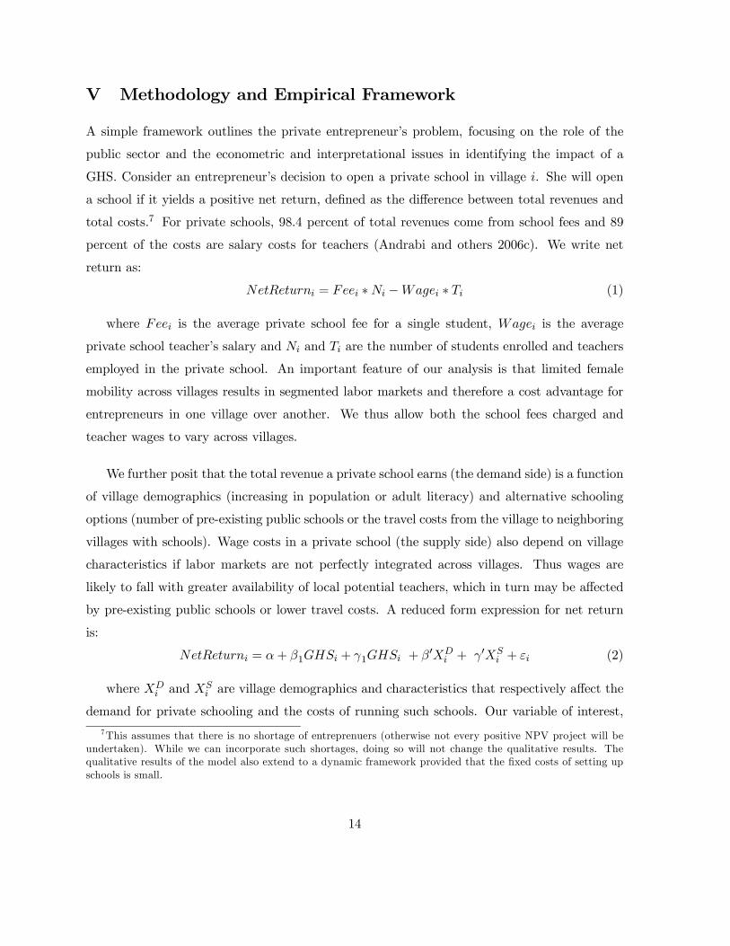
V Methodology and Empirical Framework

A simple framework outlines the private entrepreneur’s problem, focusing on the role of the

public sector and the econometric and interpretational issues in identifying the impact of a

GHS. Consider an entrepreneur’s decision to open a private school in village i. She will open

a school if it yields a positive net return, defined as the difference between total revenues and

total costs.7 For private schools, 98.4 percent of total revenues come from school fees and 89

percent of the costs are salary costs for teachers (Andrabi and others 2006c). We write net

return as:

NetReturni = Feei ∗Ni −Wagei ∗ Ti (1)

where Feei is the average private school fee for a single student, Wagei is the average

private school teacher’s salary and Ni and Ti are the number of students enrolled and teachers

employed in the private school. An important feature of our analysis is that limited female

mobility across villages results in segmented labor markets and therefore a cost advantage for

entrepreneurs in one village over another. We thus allow both the school fees charged and

teacher wages to vary across villages.

We further posit that the total revenue a private school earns (the demand side) is a function

of village demographics (increasing in population or adult literacy) and alternative schooling

options (number of pre-existing public schools or the travel costs from the village to neighboring

villages with schools). Wage costs in a private school (the supply side) also depend on village

characteristics if labor markets are not perfectly integrated across villages. Thus wages are

likely to fall with greater availability of local potential teachers, which in turn may be affected

by pre-existing public schools or lower travel costs. A reduced form expression for net return

is:

NetReturni = α+ β1GHSi + γ1GHSi + β XDi + γ XS

i + εi (2)

where XDi and XS

i are village demographics and characteristics that respectively affect the

demand for private schooling and the costs of running such schools. Our variable of interest,

7This assumes that there is no shortage of entreprenuers (otherwise not every positive NPV project will beundertaken). While we can incorporate such shortages, doing so will not change the qualitative results. Thequalitative results of the model also extend to a dynamic framework provided that the fixed costs of setting upschools is small.

14

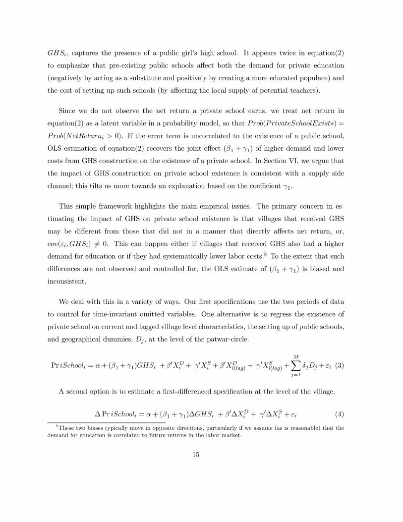
GHSi, captures the presence of a public girl’s high school. It appears twice in equation(2)

to emphasize that pre-existing public schools affect both the demand for private education

(negatively by acting as a substitute and positively by creating a more educated populace) and

the cost of setting up such schools (by affecting the local supply of potential teachers).

Since we do not observe the net return a private school earns, we treat net return in

equation(2) as a latent variable in a probability model, so that Prob(PrivateSchoolExists) =

Prob(NetReturni > 0). If the error term is uncorrelated to the existence of a public school,

OLS estimation of equation(2) recovers the joint effect (β1 + γ1) of higher demand and lower

costs from GHS construction on the existence of a private school. In Section VI, we argue that

the impact of GHS construction on private school existence is consistent with a supply side

channel; this tilts us more towards an explanation based on the coefficient γ1.

This simple framework highlights the main empirical issues. The primary concern in es-

timating the impact of GHS on private school existence is that villages that received GHS

may be different from those that did not in a manner that directly affects net return, or,

cov(εi,GHSi) = 0. This can happen either if villages that received GHS also had a higher

demand for education or if they had systematically lower labor costs.8 To the extent that such

differences are not observed and controlled for, the OLS estimate of (β1 + γ1) is biased and

inconsistent.

We deal with this in a variety of ways. Our first specifications use the two periods of data

to control for time-invariant omitted variables. One alternative is to regress the existence of

private school on current and lagged village level characteristics, the setting up of public schools,

and geographical dummies, Dj, at the level of the patwar-circle.

Pr iSchooli = α+ (β1+ γ1)GHSi +β XDi + γ XS

i +β XDi(lag)+ γ XS

i(lag)+M

j=1

δjDj + εi (3)

A second option is to estimate a first-differenced specification at the level of the village.

∆Pr iSchooli = α+ (β1 + γ1)∆GHSi + β ∆XDi + γ ∆XS

i + εi (4)

8These two biases typically move in opposite directions, particularly if we assume (as is reasonable) that thedemand for education is correlated to future returns in the labor market.

15

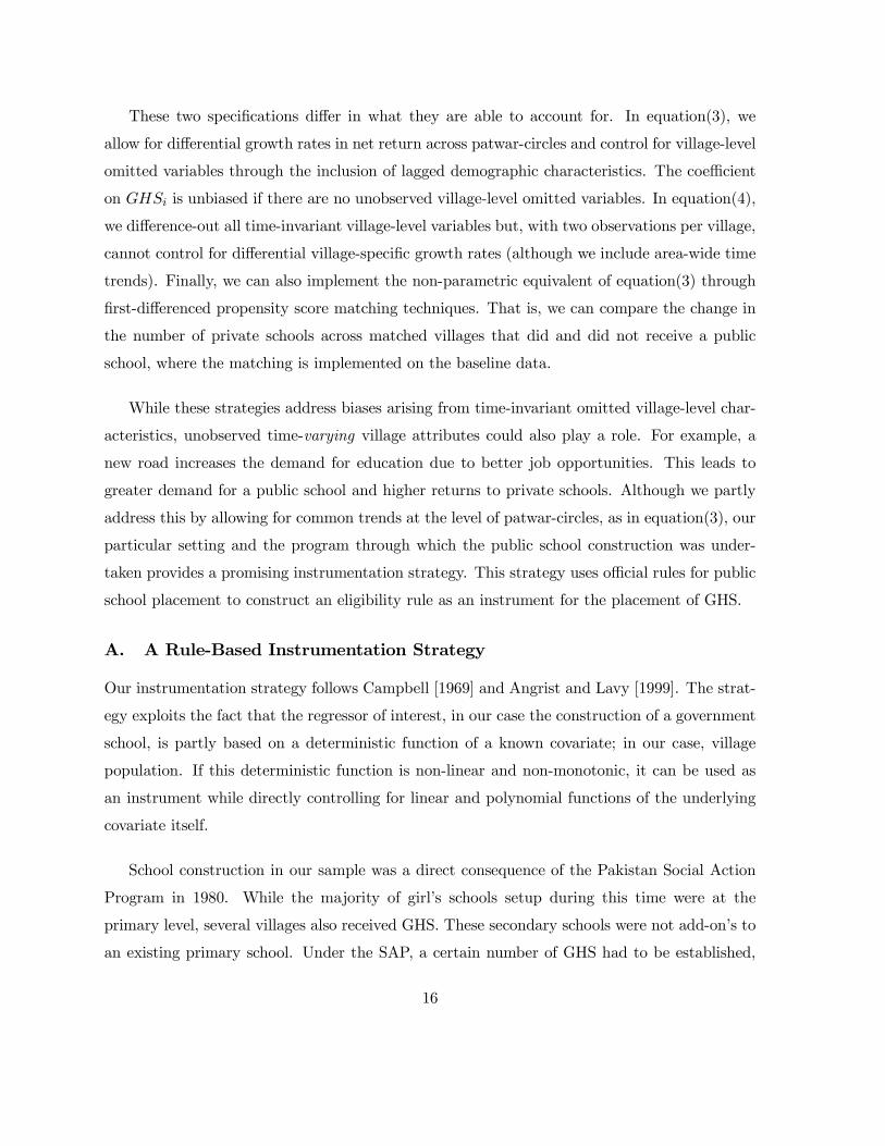
These two specifications differ in what they are able to account for. In equation(3), we

allow for differential growth rates in net return across patwar-circles and control for village-level

omitted variables through the inclusion of lagged demographic characteristics. The coefficient

on GHSi is unbiased if there are no unobserved village-level omitted variables. In equation(4),

we difference-out all time-invariant village-level variables but, with two observations per village,

cannot control for differential village-specific growth rates (although we include area-wide time

trends). Finally, we can also implement the non-parametric equivalent of equation(3) through

first-differenced propensity score matching techniques. That is, we can compare the change in

the number of private schools across matched villages that did and did not receive a public

school, where the matching is implemented on the baseline data.

While these strategies address biases arising from time-invariant omitted village-level char-

acteristics, unobserved time-varying village attributes could also play a role. For example, a

new road increases the demand for education due to better job opportunities. This leads to

greater demand for a public school and higher returns to private schools. Although we partly

address this by allowing for common trends at the level of patwar-circles, as in equation(3), our

particular setting and the program through which the public school construction was under-

taken provides a promising instrumentation strategy. This strategy uses official rules for public

school placement to construct an eligibility rule as an instrument for the placement of GHS.

A. A Rule-Based Instrumentation Strategy

Our instrumentation strategy follows Campbell [1969] and Angrist and Lavy [1999]. The strat-

egy exploits the fact that the regressor of interest, in our case the construction of a government

school, is partly based on a deterministic function of a known covariate; in our case, village

population. If this deterministic function is non-linear and non-monotonic, it can be used as

an instrument while directly controlling for linear and polynomial functions of the underlying

covariate itself.

School construction in our sample was a direct consequence of the Pakistan Social Action

Program in 1980. While the majority of girl’s schools setup during this time were at the

primary level, several villages also received GHS. These secondary schools were not add-on’s to

an existing primary school. Under the SAP, a certain number of GHS had to be established,

16

and the government could do one of three things: (a) they could either not set up any school,

(b) they could construct a girl’s primary school or, (c) they could construct a GHS that also

included a primary section. In this sense, the construction of a GHS really meant that the

building and sanctioning of teachers followed both the protocols for a primary and secondary

school–there would be more classrooms and more teachers, although in the initial years, the

number of children in the secondary classes was likely to be very low. Reflecting this design,

out of the 328 villages in our sample that received a GHS between 1981 and 2001, only 31 had

a pre-existing girls’ primary school; in all the rest, the secondary and primary sections of the

school were constructed simultaneously.

Of interest to us is that there were specific guidelines for where these schools could (and

could not) be built. For GHS the official yardstick for the opening of new schools was that

(i) the population of the village be no less than 500 (ii) there should be no government GHS

within a 10 km radius and (iii) the village would have to provide 16 kanals of land.

In order to exploit the nonlinearity in these guidelines we construct a binary assignment rule,

Rulei, that exploits the first two guidelines. Within our sample restriction, Rulei is assigned

a value 1 if (and only if) the village’s population in 1981 was greater than 500 and it was the

largest village (in terms of 1981 population) amongst nearby villages. The latter captures the

radius criteria: if a village is not the largest village amongst its neighbors, it is likely that its

neighbor would receive a public school first given the stated preference for population in the

construction of schools. Provided this school is near enough, the village will be less likely to

receive its own public school.9

Ideally we would have liked to use actual distances between villages. In the absence of

geographical data, we proxy this by including all the villages that are in the same “patwar

circle” (PC) as approximating the radius conditions of the rule. In terms of actual land area,

this is a reasonable approximation–given the size of the province and the number of patwar

circles, a back of the envelope calculation shows that a school within every patwar circle would

(roughly) satisfy the radius requirements of the rule. Our instrument then takes a particularly

9Another alternative is to use the radius-rule directly and assign rulei = 0 if there is a village in the patwar-circle that has a GHS. This is problematic since we are worried about the endogenous placement of GHS in thefirst place.

17

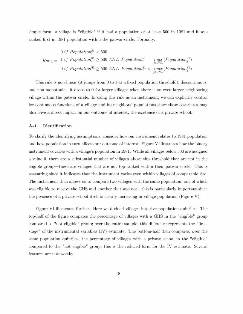
simple form: a village is "eligible" if it had a population of at least 500 in 1981 and it was

ranked first in 1981 population within the patwar-circle. Formally:

Rulei =

0 if Population81i < 500

1 if Population81i ≥ 500 AND Population81i = maxj∈PCi

(Population81j )

0 if Population81i ≥ 500 AND Population81i < maxj∈PCi

(Population81j )

This rule is non-linear (it jumps from 0 to 1 at a fixed population threshold), discontinuous,

and non-monotonic–it drops to 0 for larger villages when there is an even larger neighboring

village within the patwar circle. In using this rule as an instrument, we can explicitly control

for continuous functions of a village and its neighbors’ populations since these covariates may

also have a direct impact on our outcome of interest, the existence of a private school.

A-1. Identification

To clarify the identifying assumptions, consider how our instrument relates to 1981 population

and how population in turn affects our outcome of interest. Figure V illustrates how the binary

instrument covaries with a village’s population in 1981. While all villages below 500 are assigned

a value 0, there are a substantial number of villages above this threshold that are not in the

eligible group–these are villages that are not top-ranked within their patwar circle. This is

reassuring since it indicates that the instrument varies even within villages of comparable size.

The instrument then allows us to compare two villages with the same population, one of which

was eligible to receive the GHS and another that was not–this is particularly important since

the presence of a private school itself is clearly increasing in village population (Figure V).

Figure VI illustrates further. Here we divided villages into five population quintiles. The

top-half of the figure compares the percentage of villages with a GHS in the "eligible" group

compared to "not eligible" group; over the entire sample, this difference represents the "first-

stage" of the instrumental variables (IV) estimate. The bottom-half then compares, over the

same population quintiles, the percentage of villages with a private school in the "eligible"

compared to the "not eligible" group; this is the reduced form for the IV estimate. Several

features are noteworthy.

18

First, the instrument varies in every population quintile (we obtain similar results with

population deciles) except for the first, which consists of villages below the 500 threshold.

Thus, it is likely that our results are not driven by one particular population group. Second, for

all population quintiles the first-stage indicates a higher probability of receiving a GHS if the

village is in the eligible group. Third, in contrast to the rank rule, the threshold rule (villages less

than 500 were not supposed to receive a GHS) was not applied. A number of villages below the

500 threshold received a GHS and, rather than a discontinuity at 500, there is an almost linear

increase in the probability of receiving a GHS with population. Further comparisons around

the 500 threshold confirm the lack of discontinuities that the rule suggests–our identification

therefore is driven by the population rank-rule.10

Our strategy thus compares two villages with the same population but with different pop-

ulation ranks within the patwar circle. The exclusion restriction is that, for two villages with

the same population, the relative population rank of the village within the patwar circle does

not affect the probability of having a private school, except through GHS construction.

We can think of two reasons why this exclusion restriction may fail. If private school

entrepreneurs search for the highest returns and choose among villages within a patwar circle

(but not a broader area), they will likely choose the village with the highest population. This

assumes: (a) that there is a shortage of (local) entrepreneurs, so that even in villages where

the net present value of setting up a private school is positive, a school is not set up and (b)

that private entrepreneurs need not be resident in the village where they set up the school.

Towards ruling out such explanations, we construct a falsification test below and show that our

instrument has no predictive power in patwar-circles where no GHS were built, suggesting that

the population rank of a village plays a role only if the PC also received a GHS.

Our exclusion restriction could also fail if the government used the same rules for allocating

other investments that may affect the return to private schooling in the village. We deal

with this in two ways. First, in all specifications, we control for the presence of all types of

government schools in addition to GHS, which could affect the probability of private school

10 In robustness checks, we repeat the IV specifications without the threshold rule and replicate the resultsreported below.

19

existence.11 Second, we include regressors that are plausible measures of other government

investment, such as electrification and water-supply. We find no evidence that the rank of the

village affected the level of government investment, either in means-comparisons or in regression

specifications. Indeed, other government investments such as water and electricity are slightly

lower in higher population rank villages, although the coefficients are small and insignificant.

A final econometric issue is that our treatment (the construction of a public school) and

dependent variable (the existence of a private school) are binary. Early work in the choice of

specifications suggests that linear instrumental variables estimates are not very different from

more structured models in such settings (Angrist 1991). In addition however our treatment

probabilities are low. At low treatment probabilities the choice of specification will make a

difference since the cumulative distributions of the uniform and normal will differ.12

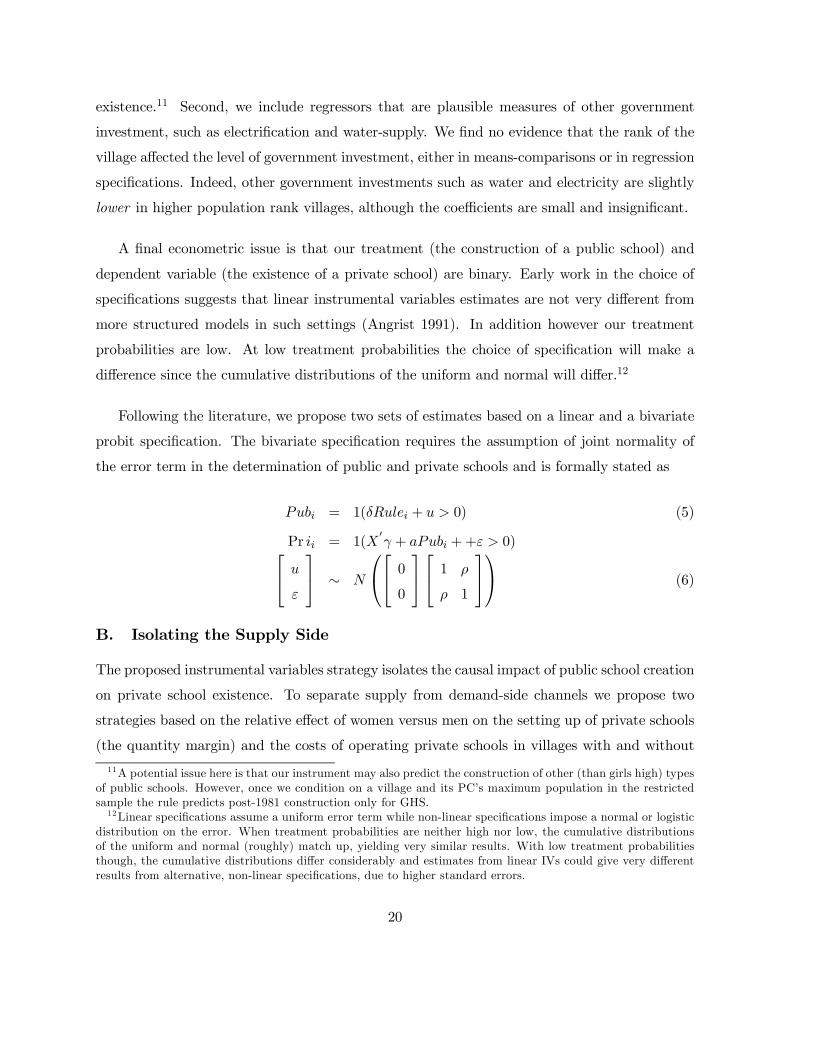
Following the literature, we propose two sets of estimates based on a linear and a bivariate

probit specification. The bivariate specification requires the assumption of joint normality of

the error term in the determination of public and private schools and is formally stated as

Pubi = 1(δRulei + u > 0) (5)

Pr ii = 1(X γ + aPubi ++ε > 0) uε

∼ N

00

1 ρ

ρ 1

(6)

B. Isolating the Supply Side

The proposed instrumental variables strategy isolates the causal impact of public school creation

on private school existence. To separate supply from demand-side channels we propose two

strategies based on the relative effect of women versus men on the setting up of private schools

(the quantity margin) and the costs of operating private schools in villages with and without

11A potential issue here is that our instrument may also predict the construction of other (than girls high) typesof public schools. However, once we condition on a village and its PC’s maximum population in the restrictedsample the rule predicts post-1981 construction only for GHS.12Linear specifications assume a uniform error term while non-linear specifications impose a normal or logistic

distribution on the error. When treatment probabilities are neither high nor low, the cumulative distributionsof the uniform and normal (roughly) match up, yielding very similar results. With low treatment probabilitiesthough, the cumulative distributions differ considerably and estimates from linear IVs could give very differentresults from alternative, non-linear specifications, due to higher standard errors.

20

GHS (the price margin).13

For the quantity margin, a supply-side channel suggests several patterns. If the teachers’

supply effect is important compared to parental demand, the impact of public high schools

should be larger than that of public primary schools. The assumption is that while an adult

with only primary level education is not a suitable teaching candidate (98 percent of private

school teachers have at least secondary education), the difference in parental demand for primary

education may not differ substantially across parents with primary versus secondary education.

We thus consider the differential impact of public schools by level (primary versus high) and

gender (boys versus girls). We expect high schools to be more important than primary schools,

and, since teachers in private schools are primarily women, girl’s high schools to have a larger

impact than boy’s high schools.

We also focus directly on the supply of educated men and women. We examine whether

there are more adult women with higher education in treatment villages (that received a girl’s

high school) and, in turn, whether the existence of a private school increases with the fraction

of adult women with higher education in the village (both absolutely and relative to adult men

with higher education).

While results in the expected direction from these tests lend support to the supply-side

channel, alternative explanations based on demand channels are possible: Several studies doc-

ument the relative importance of women compared to men for investment in the human capital

of their children, and secondary education could have a differential impact on parental demand

compared to primary education.

A more compelling test is based on cost differences in private schools. The price implications

of the supply and demand-side stories differ. If the existence of a private school responds to an

13One possibility is to use the variation in the timing of the public school construction. If supply-side storiesare correct, we would expect a private school to emerge 5-8 years after the construction of the girl’s high school.Unfortunately, that data are too limited to exploit such variation. We require villages with both private schoolsand girl’s high schools. Since only 324 villages received a girl’s high school and of these 30 percent had a privateschool, we are unable to identify any discontinuities off the 100 or so villages that have both. Another possibilityis to check whether there is a difference in the existence of a private school based on years of exposure to a GHS.Here we do find some evidence that less than 5 years of exposure has no effect on the likelihood of private schoolexistence. In particular, private schools exist in 18 percent of villages with less than 5 years of exposure to aGHS (compared to 12 percent among the control), and in 33 percent of those with 5 or more years.

21

increase in the supply of teachers, the wage-bill of private schools should be lower in villages

with public girls’ high schools. In the absence of such a school, the entrepreneur would either

have to bring in teachers from outside (if possible) and pay for the compensating differential

and travel costs; alternatively she would have to pay higher wages for educated male teachers.14

We test whether our data support this hypothesis. One complication is that we observe non-

missing values of the wage-bill only in villages where private schools exist, and this selection

problem will underestimate the true wage-bill differences in the population.15 We follow two

approaches to address the selection problem. We use a Heckman selection model, where the

selection stage is the probability of observing a positive wage, which corresponds to having

a private school in the village. Another alternative is to use the "control-function" approach

(Angrist 1995), where we condition on the predicted probability of observing a non-missing

value of the wage-bill in the wage equation. Details of both approaches are in the Appendix.

In either approach, identification is based on the non-linearity of the selection equation

(see Duflo 2001 as an example). Augmenting the instrument set with potential candidates

that are correlated to the probability of setting up a private school (where we observe wages)

but uncorrelated to the wage-bill for entrepreneurs setting up a private school can help in

identification and the efficiency of the estimator. Following the industrial-organization work by

Dowes and Greenstein (1996), we propose using the number of public boys primary schools as an

additional instrument in the selection equation. In the presence of competitive effects, private

schools should be less likely to setup in villages where there are public boy’s primary schools;

additionally, such schools are unlikely to affect the wage-bill of the entrepreneur directly.

This instrument might be less than perfect. If boy’s primary schools are differentially located

in villages where the returns to education are low or if men and women compete directly for14An alternative would be to look at wages of secondary-school educated women who may or may not be

teachers. The only available data source is the Pakistan Integrated Household Survey. Unfortunately, giventhe small number of villages that received a GHS, the available sample sizes are too small–with the samplerestrictions in our paper, we find only 3 villages in the treatment and 31 villages in the control set for these data.15Consider the following wage-bill distributions in villages with and without GHS.

[5, 6, 7, 8, 9, 10] (Without GHS)

[3, 4, 5, 6, 7, 8] (With GHS)

In the absence of any demand effects, suppose that private schools can only afford to set up in villages where thewage-bill is below 7. Thus, where we observe the wage-bill, E(WBi|WBi is non missing, no GHS) - E(WBi|WBiis non missing, GHS) is lower than the uncensored E(WBi|no GHS) - E(WBi|GHS).

22

positions in the labor market for teachers, there could be a direct relationship between such

schools and the wage-bill that entrepreneurs face. In our case, the additional instrument serves

as a "robustness" check to the identification based only on non-linearities in the selection

equation.

Finally, if there are simultaneous changes in the demand for schooling induced by girls’

high schools, our estimate of the effect of GHS on the wage-bill will always represent a lower

bound. To see this, reconsider the example in Footnote 11 and suppose the GHS increases

the demand for private education, so that the minimum wage-bill at which private schools

are profitable in villages with GHS is higher than those without GHS. In this case, E(WBi|noGHS) - E(WBi|GHS) recovers the joint-effect of a lower wage-bill and increases in demand–wecannot separate out these two effects.

VI Results

A. Baseline Differences

Recall our sample is the set of villages in patwar circles where no village had a GHS in 1981, the

date of our baseline data. We define our treatment villages as those that received a GHS and

control villages as those that either did not receive a girls’ school at all, or those that received

a girls’ primary school. What did our treatment and control villages look like in 1981? Table

III shows that in terms of female literacy, male literacy, gender ratios, and basic demographic

attributes such as the percentage of male and female infants (less than age 4) and children (ages

5 to 14) there were no significant differences between treatment and control villages. Consistent

with the stated rule, the population in treatment villages was almost twice as large as in the

control. Using measures of infrastructure and public goods in these villages from the 1998

census shows little wealth differences (Appendix Table I). In fact judging from the percentage

of households that own land in 1998, treatment villages fare slightly worse than control villages.

B. OLS and First-Difference Specifications

Table IV presents results from our primary specification. The probit specification shows that

a pre-existing girl’s public secondary school increases the probability of a private school in the

23

village by 9.7 percentage points (Column 1, Table 3). Since 12 percent of all control villages

have a private school, this represents an 80 percent increase. An equally significant determinant

of private school existence is village population; taken literally, the girl’s secondary school effect

is similar in magnitude to increasing village population by 2000 individuals (coincidentally a

one standard-deviation increase in population). The estimated impact remains significant at

the 1 percent level when we introduce a full set of village level controls including exposure to

other types of public schools, although the point-estimate is somewhat attenuated (Column

2, Table IV). Introducing geographical dummies for patwar circles as in equation(3) increases

the estimate and significance with magnitudes very similar to the first specification (Column 3,

Table IV).

Following equation(4), Columns (4) and (5) control for time-invariant village effects by first-

differencing the data at the village level. Interestingly, the effect of girl’s high school on private

school increases to almost 15 percentage points. This suggests some evidence of selection,

although in the opposite direction to what one might expect: Villages that received GHS were

also those where the returns to private schools were systematically lower.

Column (5) presents further evidence of such selection by including cluster specific time-

trends in the first-difference specification. The GHS effect increases further to 17.4 percentage

points. Since the specification is already in first differences, introducing cluster specific time-

trends accounts for unobserved time-varying factors that are common across villages in the

cluster and may affect both the likelihood of GHS provision and private school returns. Thus

if a selection concern was that a village that received a road saw greater returns to education

and hence greater demand for public (and private) schooling, as long as this road affected

neighboring villages similarly, the estimate of GHS on private schools is unbiased and consistent.

Non-parametric (propensity-score) techniques yield similar results. A pre-existing girl’s high

school increases private school existence probabilities by 11 to 14 percentage points depending

on whether we use local linear regression or kernel matching (results available with authors).

These results suggest two patterns: if time-varying omitted-variables play a small role, GHS

are critical for the future development of private schools, both absolutely and relative to other

types of schools. Furthermore, the difference in the estimated coefficient using the cross-section

and panel lead us to believe that GHS were not distributed randomly–they were systematically

24

targeted to villages where private schools were less likely to emerge. The next section explores

whether selection on time-varying characteristics was also important.

C. Instrumental Variable Specifications

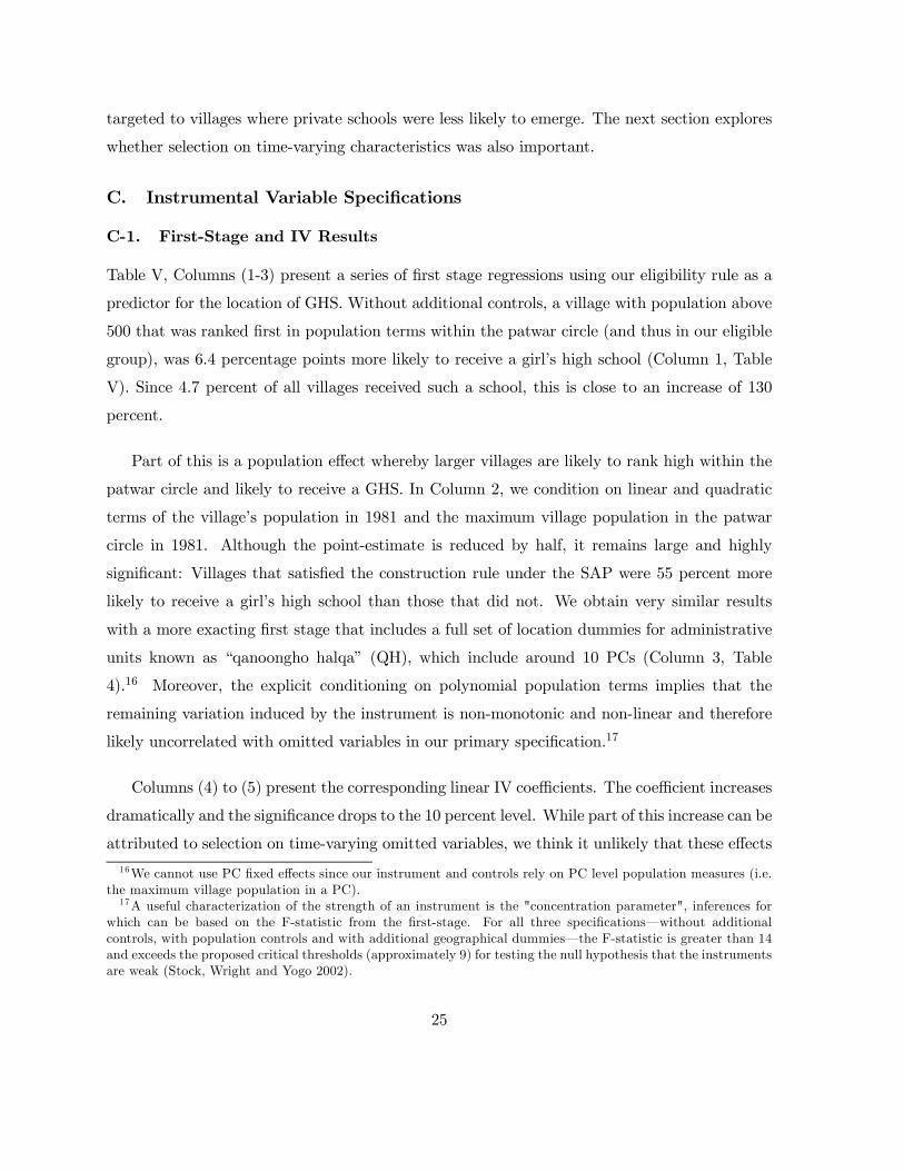
C-1. First-Stage and IV Results

Table V, Columns (1-3) present a series of first stage regressions using our eligibility rule as a

predictor for the location of GHS. Without additional controls, a village with population above

500 that was ranked first in population terms within the patwar circle (and thus in our eligible

group), was 6.4 percentage points more likely to receive a girl’s high school (Column 1, Table

V). Since 4.7 percent of all villages received such a school, this is close to an increase of 130

percent.

Part of this is a population effect whereby larger villages are likely to rank high within the

patwar circle and likely to receive a GHS. In Column 2, we condition on linear and quadratic

terms of the village’s population in 1981 and the maximum village population in the patwar

circle in 1981. Although the point-estimate is reduced by half, it remains large and highly

significant: Villages that satisfied the construction rule under the SAP were 55 percent more

likely to receive a girl’s high school than those that did not. We obtain very similar results

with a more exacting first stage that includes a full set of location dummies for administrative

units known as “qanoongho halqa” (QH), which include around 10 PCs (Column 3, Table

4).16 Moreover, the explicit conditioning on polynomial population terms implies that the

remaining variation induced by the instrument is non-monotonic and non-linear and therefore

likely uncorrelated with omitted variables in our primary specification.17

Columns (4) to (5) present the corresponding linear IV coefficients. The coefficient increases

dramatically and the significance drops to the 10 percent level. While part of this increase can be

attributed to selection on time-varying omitted variables, we think it unlikely that these effects

16We cannot use PC fixed effects since our instrument and controls rely on PC level population measures (i.e.the maximum village population in a PC).17A useful characterization of the strength of an instrument is the "concentration parameter", inferences for

which can be based on the F-statistic from the first-stage. For all three specifications–without additionalcontrols, with population controls and with additional geographical dummies–the F-statistic is greater than 14and exceeds the proposed critical thresholds (approximately 9) for testing the null hypothesis that the instrumentsare weak (Stock, Wright and Yogo 2002).

25

are as large as the estimates suggests. Column (6) assesses whether functional specification

plays a role. We implement a bivariate probit specification following equation (5) and report

the marginal impact of girl’s high school on the existence of a private school. The standard errors

are bootstrapped at sample values of other variables (alternative standard errors calculated at

the mean of the sample-value for other variables yield similar results). The point-estimate from

the bivariate probit is half that of the linear IV and significant at the 5 percent level. The

estimate suggests selection on unobservable variables, and is double what we obtain with the

first-differenced specification: Constructing a GHS increases the probability of a private school

in the village by 36 percentage points, or over 300 percent.

C-2. Linear IV and Biprobit: Further Robustness Tests

Why are there large differences between the biprobit and the linear IV estimator? While

the instrument has high predictive power in the first-stage, the probability of the treatment

is low. At low treatment probabilities, standard-errors of the linear IV estimate are high,

while the bivariate probit is typically more efficient. In Monte-Carlo simulations, we consider

various treatment (T) and outcome (Y) probabilities and examine the efficiency of linear IV

and biprobit estimates (Das and Lokshin 2006). When treatment (or outcome) probabilities

are very low/high, the standard-error of the linear IV estimator increases dramatically so that

linear IV and biprobit point estimates differ substantially. In the context of our data, these

deviations are indeed large with 87 percent of the sample concentrated in a single cell, (T=0

and Y=0).18

Further structure on the manner in which GHS were located can help understand the differ-

ence between these two estimators as well as provide evidence on the validity of the instrument.

Our final sample consists of 6968 villages, of which 2128 are in the "eligible" group (the in-

strument, Z = 1) and 4840 are in the "ineligible" group (Z = 0). However, only 328 villages

eventually received the treatment of which 60 percent are in the eligible and 40 percent are in

the ineligible group. Consistent with our interpretation of the policy rules, 96 percent of all

18The literature on the effects of Catholic schooling on graduation rates is similarly structured (very fewchildren are in Catholic schools) and encounters similar problems. In a recent paper (Altonji and others 2005), theauthors suggest that differences between the linear IV and biprobit estimator arise due to the added identificationpower from the non-linear structure of the latter. They also suggest strategies to understand the validity of theinstrument and identification in these different estimators, which motivate the robustness tests discussed here.

26

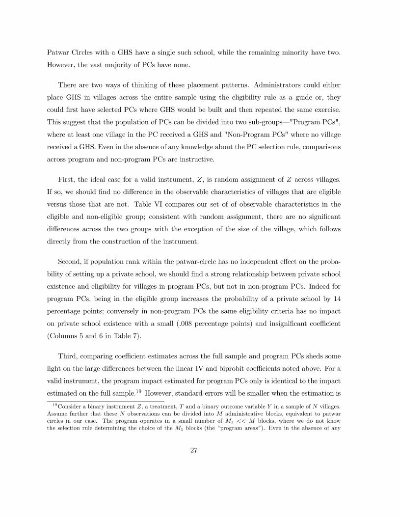
Patwar Circles with a GHS have a single such school, while the remaining minority have two.

However, the vast majority of PCs have none.

There are two ways of thinking of these placement patterns. Administrators could either

place GHS in villages across the entire sample using the eligibility rule as a guide or, they

could first have selected PCs where GHS would be built and then repeated the same exercise.

This suggest that the population of PCs can be divided into two sub-groups–"Program PCs",

where at least one village in the PC received a GHS and "Non-Program PCs" where no village

received a GHS. Even in the absence of any knowledge about the PC selection rule, comparisons

across program and non-program PCs are instructive.

First, the ideal case for a valid instrument, Z, is random assignment of Z across villages.

If so, we should find no difference in the observable characteristics of villages that are eligible

versus those that are not. Table VI compares our set of of observable characteristics in the

eligible and non-eligible group; consistent with random assignment, there are no significant

differences across the two groups with the exception of the size of the village, which follows

directly from the construction of the instrument.

Second, if population rank within the patwar-circle has no independent effect on the proba-

bility of setting up a private school, we should find a strong relationship between private school

existence and eligibility for villages in program PCs, but not in non-program PCs. Indeed for

program PCs, being in the eligible group increases the probability of a private school by 14

percentage points; conversely in non-program PCs the same eligibility criteria has no impact

on private school existence with a small (.008 percentage points) and insignificant coefficient

(Columns 5 and 6 in Table 7).

Third, comparing coefficient estimates across the full sample and program PCs sheds some

light on the large differences between the linear IV and biprobit coefficients noted above. For a

valid instrument, the program impact estimated for program PCs only is identical to the impact

estimated on the full sample.19 However, standard-errors will be smaller when the estimation is

19Consider a binary instrument Z, a treatment, T and a binary outcome variable Y in a sample of N villages.Assume further that these N observations can be divided into M administrative blocks, equivalent to patwarcircles in our case. The program operates in a small number of M1 << M blocks, where we do not knowthe selection rule determining the choice of the M1 blocks (the "program areas"). Even in the absence of any

27

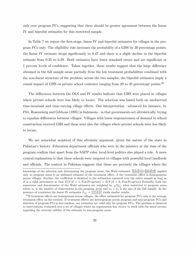
only over program PCs, suggesting that there should be greater agreement between the linear

IV and biprobit estimates for this restricted sample.

In Table 7 we repeat the first-stage, linear IV and biprobit estimates for villages in the pro-

gram PCs only. The eligibility rule increases the probability of a GHS by 30 percentage points,

the linear IV estimate drops significantly to 0.47 and there is a slight decline in the biprobit

estimate from 0.35 to 0.29. Both estimates have lower standard errors and are significant at

1 percent levels of confidence. Taken together, these results suggest that the large difference

obtained in the full sample arose partially from the low treatment probabilities combined with

the non-linear structure of the problem; across the two samples, the biprobit estimates imply a

causal impact of GHS on private school existence ranging from 29 to 35 percentage points.20

The differences between the OLS and IV results indicate that GHS were placed in villages

where private schools were less likely to locate. The selection was based both on unobserved

time-invariant and time-varying village effects. One interpretation–advanced for instance, by

Pitt, Rosenzweig and Gibbons (1995) in Indonesia–is that governments act altruistically, trying

to equalize differences between villages. Villages with lower responsiveness of demand to school

construction received GHS and these were also the villages where private schools were less likely

to locate.

We are somewhat sceptical of this altruistic argument, given the nature of the state in

Pakistan’s history. Education department officials who were in the ministry at the time of the

program confirm that apart from the SAPP rules, local-level politics also played a role. A more

cynical explanation is that these schools were targeted to villages with powerful local landlords

and officials. The context in Pakistan suggests that these are precisely the villages where the

knowledge of the selection rule determining the program areas, the Wald estimator E(Y |Z=1)−E(Y |Z=0)E(T |Z=1)−E(T |Z=0) applied

only to program areas is an unbiased estimate of the treatment effect, if the treatment effect is homogeneousacross villages. Further, the coefficient is identical to the estimation repeated over the entire sample as long asZ is a valid instrument so that E(Y |Z = 1, NonPr ogram) = E(Y |Z = 0, NonPr ogram) Formally, both thenumerator and denominator of the Wald estimator are weighted by n1

n1+n2when restricted to program areas

where n1 is the number of observations in the program areas and n1 + n2 is the size of the full sample. In thepresence of covariates the linear IV estimator βIV =

Cov(Y,Z)Cov(Y,T ) yields similar results.

20 If treatment effects are homogenous across villages, the effect estimated for program PCs only is the averagetreatment effect on the treated. If treatment effects are heterogenous across program and non-program PCs andselection of program PCs is non-random, our estimates are valid only for program PCs. The problem is identicalto interventions evaluated over a set of villages where an organization has chosen to work with the usual caveatsregarding the external validity of the estimate to non-program areas.

28

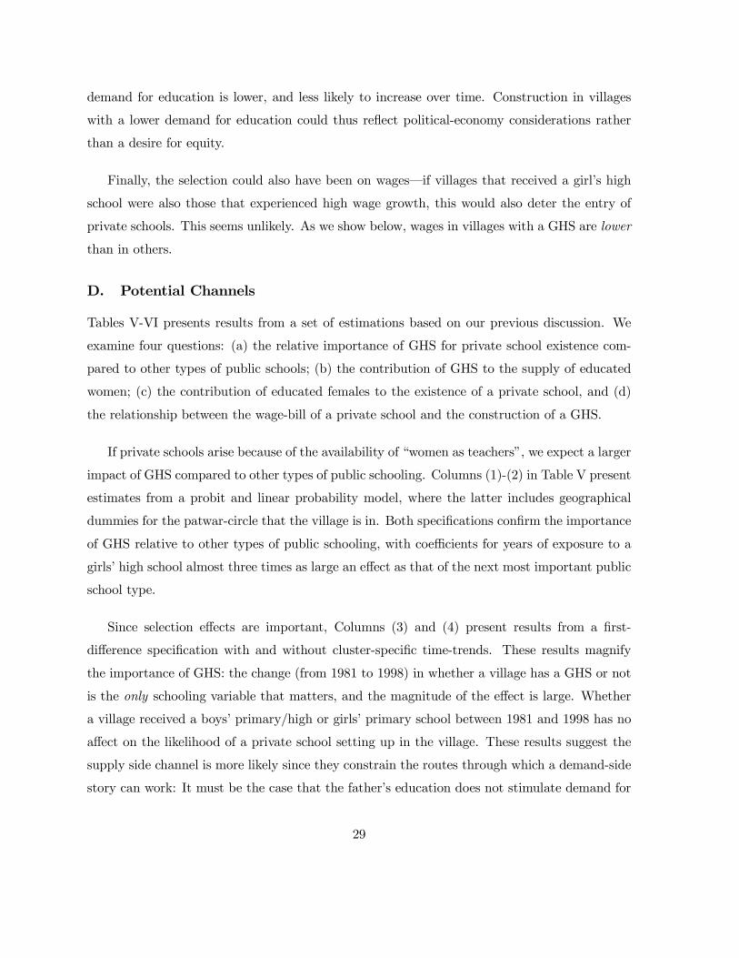
demand for education is lower, and less likely to increase over time. Construction in villages

with a lower demand for education could thus reflect political-economy considerations rather

than a desire for equity.

Finally, the selection could also have been on wages–if villages that received a girl’s high

school were also those that experienced high wage growth, this would also deter the entry of

private schools. This seems unlikely. As we show below, wages in villages with a GHS are lower

than in others.

D. Potential Channels

Tables V-VI presents results from a set of estimations based on our previous discussion. We

examine four questions: (a) the relative importance of GHS for private school existence com-

pared to other types of public schools; (b) the contribution of GHS to the supply of educated

women; (c) the contribution of educated females to the existence of a private school, and (d)

the relationship between the wage-bill of a private school and the construction of a GHS.

If private schools arise because of the availability of “women as teachers”, we expect a larger

impact of GHS compared to other types of public schooling. Columns (1)-(2) in Table V present

estimates from a probit and linear probability model, where the latter includes geographical

dummies for the patwar-circle that the village is in. Both specifications confirm the importance

of GHS relative to other types of public schooling, with coefficients for years of exposure to a

girls’ high school almost three times as large an effect as that of the next most important public

school type.

Since selection effects are important, Columns (3) and (4) present results from a first-

difference specification with and without cluster-specific time-trends. These results magnify

the importance of GHS: the change (from 1981 to 1998) in whether a village has a GHS or not

is the only schooling variable that matters, and the magnitude of the effect is large. Whether

a village received a boys’ primary/high or girls’ primary school between 1981 and 1998 has no

affect on the likelihood of a private school setting up in the village. These results suggest the

supply side channel is more likely since they constrain the routes through which a demand-side

story can work: It must be the case that the father’s education does not stimulate demand for

29

their children’s education and also that primary schooling for mothers is not enough. The only

mothers who demand more education for their children are those who have eight or more years

of schooling–indeed, there must be strong nonlinearity in the demand for children’s education

and mother’s schooling.

Columns (5)-(8) present the next logical step. We assess the correlation between educated

women and the presence of a GHS for a variety of specifications. In all specifications, a GHS

increases the percentage of adult women with higher levels of education (equal to or more than

8 years of schooling) by 1.5-2.2 percentage points and the estimated increases are significant at

the 1 percent level of confidence. While this may appear as a small effect, only 1.3 percent of

all women in the average village in 1981 had higher levels of education. Therefore a GHS more

than doubles this percentage.

Columns (9)-(12) in Panel B examines the importance of highly educated women for the

existence of a private school. Are such women more important than similarly educated men?

Restricted mobility and employment opportunities for women suggests that educated women

should have a bigger impact than educated men, since their wage rates will be lower. While

the effect of educated men is only slightly smaller in the basic probit specification in column

(9), this difference between educated men and women increases substantially once we control

for geographical location, suggesting that part of the estimated coefficient on male education

was due to omitted geographical characteristics. For our preferred first-difference specification,

the impact of women with 8 or more years of schooling remains as strong while the percentage

of educated males has no impact on the existence of a private school.

Table VI then examines the wage-bill in private schools across villages with and without

GHS using data from the private school census.21 Column (1) presents the OLS results in the

sample of villages for which wage data is not missing.22 The results are large and significant

21 Ideally, data on the wages of women with high school education (i.e. the level necessary to become primaryschool teachers) would avoid the selection problem of missing data in villages without private schools. However,there are few sources that provide such village level wage estimates. Moreover, very few women work in non-farmactivities so that sample sizes are typically small. While these wages cannot be separated by gender, since thevast majority of private school teachers are women, the wage bill is likely to reflect wages to skilled women.22This is slightly smaller than the number of villages where there is a private school since in a few cases in the

PEIP data private schools did not report wages.

30

and in the direction predicted by the supply-side channel. Private schools in villages with a

GHS report an 18 percent lower wage-bill.23

Columns (2)-(5) correct for selection into the sample. Columns (2)-(3) present results from

estimating a Heckman selection model and Columns (4)-(5) use the alternate “control func-

tion” approach (see Appendix). Columns (2) and (4) identify solely of non-linearities, whereas

Columns (3) and (5) introduce an additional instrument for the selection stage–the number of

government boys’ primary schools in the village. The results are similar to the OLS estimates

suggesting that selection into the non-zero wage sample is of limited importance.

Together with the results on the quantity margin–that GHS and not other forms of public

schooling, and female higher education and not male higher education, affect private school

existence, the wage-bill results present direct evidence that the supply-side “women-as-teachers”

channel is important in determining where private schools are setup. Given localized labor

markets for women, GHS reduce wages in the village for educated women by increasing the

relative supply of such women, and this in turn allows private school to exist by taking advantage

of an affordable local supply of teachers.

VII Conclusion

With 2 million adolescents in Pakistan poised to enter the labor-force each year, human capital

investments will play a large role in determining where these children will fit into a fast global-

izing world. Children in rural private schools will have learnt a lot more by the time they leave

the formal schooling system than their counterparts; at the same time, their annual education

costs will have been half as much. However, not everyone has access to private schools–children

are far more likely to attend private schools if they are located in their own village.

The causal impact of girl’s high schools on subsequent location of a private school calls for

public investment-led growth in the spirit of “big-push” arguments advanced by Rodenstein-

Rodan (1943) and Murphy, Shleifer and Vishny (1989). In contrast to the literature that calls

for larger primary school compared to secondary school investment, our findings suggest that

23Attenuation bias from a noisy measure of women’s wages (average wages in private schools), implies thatthe actual differential may be even higher.

31

both play a role. That the students in today’s schools are the potential repositories of human

capital for the next generation implies that low-income countries can enter a "virtuous cycle"

by investing heavily in the creation of a cohort of educated women.

The results on how girl’s high schools lead to the creation of private schools in the next

generation are a testimony to the resilience of the private sector and its ability to convert

cultural constraints–the restricted mobility and labor-market opportunities for women–into

an advantage. Villages with girl’s high schools are also those with a larger stock of educated

women, who can then teach in private schools. With limited mobility, a private school entre-

preneur becomes a virtual monopsonist when located in such a village. At one level, this seems

like a pernicious outcome: Women receive lower wages in the labor market compared to men

for the same job. At the same time, these cost savings are directly passed on to the children

who study in these schools; in the absence of this labor market distortion, it is unclear whether

these schools could have catered to the children from low and middle-income families that are

currently enrolled in them.

The results also provide a fascinating glimpse of education in high-income countries during

the early to mid-twentieth century. Recent papers concerned about the decline in high-quality

teachers in US public schools point to greater employment opportunities and increasing pay

for women in non-teaching fields (Hoxby (2004) also finds that wage-compression due to union-

ization plays a large role). The rise of private schools in Pakistan suggest that in low-income

countries at least, the “implicit-subsidy” to education from low female labor-force participation

is alive and kicking.

32

AppendixSelection Issues in the Wage Bill

Since we only observe the wage bill in villages where there is a private school, a concern

described in the main text is that simple OLS estimates may be biased if such selection is

not accounted for. Here we provide details on two approaches we use in the paper to address

such concerns. Following Angrist (1995), the problem can be formally stated as follows. The

wage-bill is determined through a linear equation conditional on the existence of a private school

WBi = α+ βGHSi + εi (7)

and a censoring equation (denoting WBi = I as the indicator for whether WBi is non-

missing)

WBi = I{δGHSi − νi > 0} (8)

The instrument Zi determines a first stage

GHSi = γ + µZi + τ i (9)

Given the validity of the instrument, Zi, we assume that cov(τ i, Zi) = 0. Then,

E(εi|Zi,WBi = 1) = E(εi|Zi, (δγ + δµZi > νi − δτ i)

so that cov(εi, Zi) = 0 in equation(7) above. Thus, although Zi is a valid instrument for

the decision to setup a private school, it is not a valid instrument in equation(7). There are

two potential solutions.

Following Heckman (1978) if we assume that (εi, νi, τ i) are jointly normally distributed,

homoskedastic and independent of Zi, we obtain the familiar "mills-ratio" as the relevant ex-

pectation function conditional on participation. That is,

E(εi|Zi, (δγ + δµZi > νi − δτ i) = λ(δγ + δµZi)

where λ(δγ + δµZi) =−φ(λ(δγ+δµZi))Φ(λ(δγ+δµZi))

and φ(.) and Φ(.) are the density and distribution

functions of the normal distribution for νi − δτ i. This mills-ratio can is then directly included

33

in equation(7) as the appropriate selection-correction.

An alternative approach, proposed by Heckman and Robb (1986) and developed by Ahn

and Powell (1993) uses the "control-function" approach, where we condition on the predicted

probability of WBi = 1 in equation(7). In essence, this method proposes to estimate β by

using pair-wise differences in WBi for two villages (in our case) for which the non-parametric

probability of participation is very close. The approach is implemented by first estimating

equation(8) directly, and then including the predicted probability of participation (and its

polynomials) as additional controls in equation(7).

34

References

[1] Ahn, H. and J.L. Powell. 1993. “Semi-parametric Estimation of Censored Selection Models

with a Nonparametric Selection Mechanism,” Journal of Econometrics 58, 3-29.

[2] Alderman, Harold, Peter Orazem, and Elizabeth Paterno. “School Quality, School Cost

and the Public/Private School Choices of Low-Income Households in Pakistan,” Journal

of Human Resources 36(2):304-326 Spring 2001

[3] Alderman, Harold, Jooseop Kim, and Peter Orazem. “Design, Evaluation, and Sustain-

ability of Private Schools for the Poor: The Pakistan Urban and Rural Fellowship School

Experiments,” Economics of Education Review 22(3):265-274. 2003

[4] Altonji, Joseph, Todd Elder and Christoper Taber 2005. "Selection on Observed and Un-

observed Variables: Assessing the Effectiveness of Catholic Schools" forthcoming Journal

of Political Economy.

[5] Altonji, Joseph, Todd Elder and Christoper Taber 2005."An Evaluation of Instrumental

Variable Strategies for Estimating the Effects of Catholic Schools." forthcoming, Journal

of Human Resources

[6] Andrabi, Tahir, Jishnu Das, Asim Khwaja and Tristan Zajonc, 2006a, “Religious Education

in Pakistan: A Look at the Data”, forthcoming, Comparative Education Review.

[7] Andrabi and others 2006b. "Report on Learning and Educational Attainments in Pakistani

Schools. Working Paper.

[8] Andrabi, Tahir, Jishnu Das and Asim Khwaja 2006c. "Private Schooling in Pakistan:

Possibilities and Limits." Working Paper.

[9] Angrist, J. and V. Lavy, 1999. “Using Maimonedes Rule to Estimate the Effect of Class

Size on Scholastic Achievement,” Quarterly Journal of Economics, Vol. 114, No. 2, 533-575.

[10] Angrist, J. 1995.“Conditioning on the Probability of Selection to Control Selection Bias,”

NBER Technical Working Paper No. 181. Cambridge, Massachussetts.

[11] Besley, Timothy, and Stephen Coate, “Public Provision of Private Goods and the Redis-

tribution of Income.” The American Economic Review 81(4), 979-984. September 1991.

35

[12] Campbell, D.1969. ”Reforms as Experiments,” American Psychologist, XXIV, 409-429.

[13] Downes, Thomas A. and Shane M. Greenstein. 1996. "Understanding the Supply Decisions

of Nonprofits: Modeling the Location of Private Schools" Rand Journal of Economics Vol.

27(2)

[14] Downes, Thomas A. & Greenstein, Shane M. 2002. "Entry into the Schooling Market: How

is the Behaviour of Private Suppliers Influenced by Public Sector Decisions?" Bulletin of

Economic Research 54 (4), 341-371.

[15] Dulfo, E. (2001). “Schooling and Labor Market Consequences of School Construction in

Indonesia: Evidence from an Unusual Policy Experiment,” American Economic Review,

Vol. 91, No. 4.

[16] Figlio, David N. and Joe E. Stone. 1997. "School Choice and Student Performance: Are Pri-

vate Schools Really Better?" Discussion Paper 1141-97. Institute for Research on Poverty.

University of Wisconsin.

[17] Fisher, Gary. 1976. "The Identification Problem in Econometrics." Robert E. Kreiger Pub-

lishing Company, Huntington, New York.

[18] Government of Punjab, Department of Education. 2002. "Educational Management Infor-

mation System for Punjab."

[19] Government of Pakistan, 1983, Sixth Five Year Plan 1983-88, Planning Commission, Is-

lamabad

[20] Government of Pakistan, 1997, Report on the PIHS 1995-96, Islamabad

[21] Holmes, Jessica. 1999. "Measuring the Determinants of School Completion in Pakistan:

Analysis of Censoring and Selection Bias." Center Discussion Paper Number 794, Economic

Growth Center, Yale University.

[22] Heckman, J. J., and R. Robb. 1986. “Alternate Methods for Solving the Problem of Se-

lection Bias in Evaluating the Impact of Treatments on Outcomes,” in H. Wainer, ed.,

Drawing Inferences from Self-Selected Samples, New York: Springer-Verlag.

36

[23] Hoxby, Caroline M. 1994. "Do Private Schools Provide Competition for Public Schools?"

National Bureau of Economic Research Working Paper Number 4978.

[24] Hoxby, Caroline M. and Andrew Leigh. 2004. "Pulled Away or Pushed Out? Explaining the

Delhine of Teacher Aptitude in the United States." American Economic Review, Vol.93(2)

[25] Jacoby, Hanan and Ghazala Mansuri. 2006. "Crossing Boundaries: Social Distance and

the Gender Gap in Schooling in Rural Pakistan." Mimeo.

[26] Jimenez, Emmanuel and Jee-Peng Tan. 1985. "Educational development in Pakistan :

the role of user charges and private education, Volume 1." Education and training series

Discussion Paper Number EDT 16. World Bank. Washington, D.C.

[27] Jimenez, Emmanuel and Jee-Peng Tan. 1987. "Decentralized and private education : the

case of Pakistan, Volume 1." Education and training series Discussion Paper Number EDT

67. World Bank. Washington, D.C.

[28] Jimenez, Emmanuel, Marlaine E Lockheed and Vicente Paqueo. 1999. "The relative effi-

ciency of private and public schools in developing countries." World Bank Research Ob-

server. Vol. 6, no.2 (July 1991), pp. 205-218.

[29] Kingdon, Geeta. 1996. "The Quality and Efficiency of Private and Public Education: A

Case-study of Urban India." Oxford Bulletin of Economics and Statistics.

[30] Kim, Jooseop, Harold Alderman, and Peter Orazem. “Can Private School Subsidies In-

crease Schooling for the Poor? The Quetta Urban Fellowship Program,” World Bank

Economic Review 13(3):443-466. 1999

[31] Murphy, Kevin M & Shleifer, Andrei & Vishny, Robert W, 1989. "Industrialization and

the Big Push," Journal of Political Economy, University of Chicago Press, vol. 97(5), pages

1003-26.

[32] Orazem, Peter F. 2000. "The Urban and Rural Fellowship School Experiments in Pakistan:

Design, Evaluation and Sustainability." The World Bank. Washington, DC.

[33] Pitt, Mark M., Mark R. Rosenzweig and Donna M. Gibbons, 1995. “The Determinants

and Consequences of the Placement of Government Programs in Indonesia.” In D. van de

37

Walle and K. Nead, eds., Public Spending and the Poor: Theory and Evidence. Baltimore:

Johns Hopkins University Press for the World Bank.

[34] Psacharopolous, G. 2002. "Returns to Investment in Education: A Further Update." World

Bank Policy Research working paper series Number 2881. World Bank, Washington D.C.

[35] Rodenstein-Rodan, Paul. 1943. "Problems of Industrialization of Eastern and South-

Eastern Europe." Economic Journal 53 (210-211): 202-211.

[36] Stock, James H., Jonathon H. Wright and Motohiro Yogo. 2002. "A Survey of Weak Instru-

ments and Weak Identification in Generalized Method of Moments." Journal of Business

and Economic Statistics, Vol.20(4) 518:529.

[37] Tilak, Jandhyala B.G. and Ratna M. Sudarshan. 2001. "Private Schooling in Rural India."

National Council of Applied Economic Research Working Paper #WP010009. NCAER,

New Delhi, India.

[38] Tooley, James and Pauline Dixon. 2005. "Private Education is Good for the Poor." Cato

Institute. Washington DC.

[39] Tooley, James. "Private Schools for the Poor." Education Next. Fall 2005: 22-33.

[40] World Bank. 2005. "Improving Gender Outcomes: The Promise for Pakistan.". World

Bank, Washington, D.C.

38

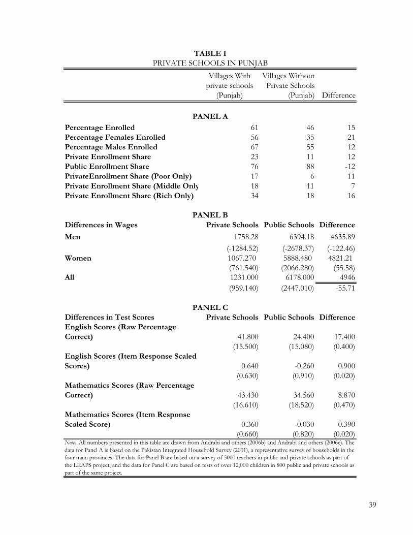
Villages With private schools

(Punjab)

Villages Without Private Schools

(Punjab) Difference

Percentage Enrolled 61 46 15Percentage Females Enrolled 56 35 21Percentage Males Enrolled 67 55 12Private Enrollment Share 23 11 12Public Enrollment Share 76 88 -12PrivateEnrollment Share (Poor Only) 17 6 11Private Enrollment Share (Middle Only 18 11 7Private Enrollment Share (Rich Only) 34 18 16

Differences in Wages Private Schools Public Schools Difference

Men 1758.28 6394.18 4635.89(-1284.52) (-2678.37) (-122.46)

Women 1067.270 5888.480 4821.21(761.540) (2066.280) (55.58)

All 1231.000 6178.000 4946(959.140) (2447.010) -55.71

Differences in Test Scores Private Schools Public Schools DifferenceEnglish Scores (Raw Percentage Correct) 41.800 24.400 17.400

(15.500) (15.080) (0.400)English Scores (Item Response Scaled Scores) 0.640 -0.260 0.900

(0.630) (0.910) (0.020)Mathematics Scores (Raw Percentage Correct) 43.430 34.560 8.870

(16.610) (18.520) (0.470)Mathematics Scores (Item Response Scaled Score) 0.360 -0.030 0.390

(0.660) (0.820) (0.020)

TABLE IPRIVATE SCHOOLS IN PUNJAB

Note: All numbers presented in this table are drawn from Andrabi and others (2006b) and Andrabi and others (2006c). The data for Panel A is based on the Pakistan Integrated Household Survey (2001), a representative survey of households in the four main provinces. The data for Panel B are based on a survey of 5000 teachers in public and private schools as part of the LEAPS project, and the data for Panel C are based on tests of over 12,000 children in 800 public and private schools as part of the same project.

PANEL B

PANEL A

PANEL C

39

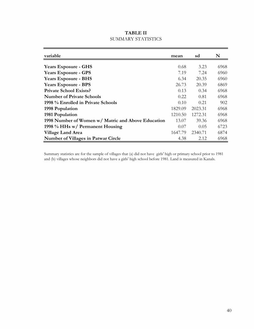
variable mean sd N

Years Exposure - GHS 0.68 3.23 6968Years Exposure - GPS 7.19 7.24 6960Years Exposure - BHS 6.34 20.35 6960Years Exposure - BPS 26.73 20.39 6869Private School Exists? 0.13 0.34 6968Number of Private Schools 0.22 0.81 69681998 % Enrolled in Private Schools 0.10 0.21 9021998 Population 1829.09 2023.31 69681981 Population 1210.50 1272.31 69681998 Number of Women w/ Matric and Above Education 13.07 39.36 69681998 % HHs w/ Permanent Housing 0.07 0.05 6723Village Land Area 1647.79 2340.71 6874Number of Villages in Patwar Circle 4.38 2.12 6968

TABLE IISUMMARY STATISTICS

Summary statistics are for the sample of villages that (a) did not have girls' high or primary school prior to 1981 and (b) villages whose neighbors did not have a girls' high school before 1981. Land is measured in Kanals.

40

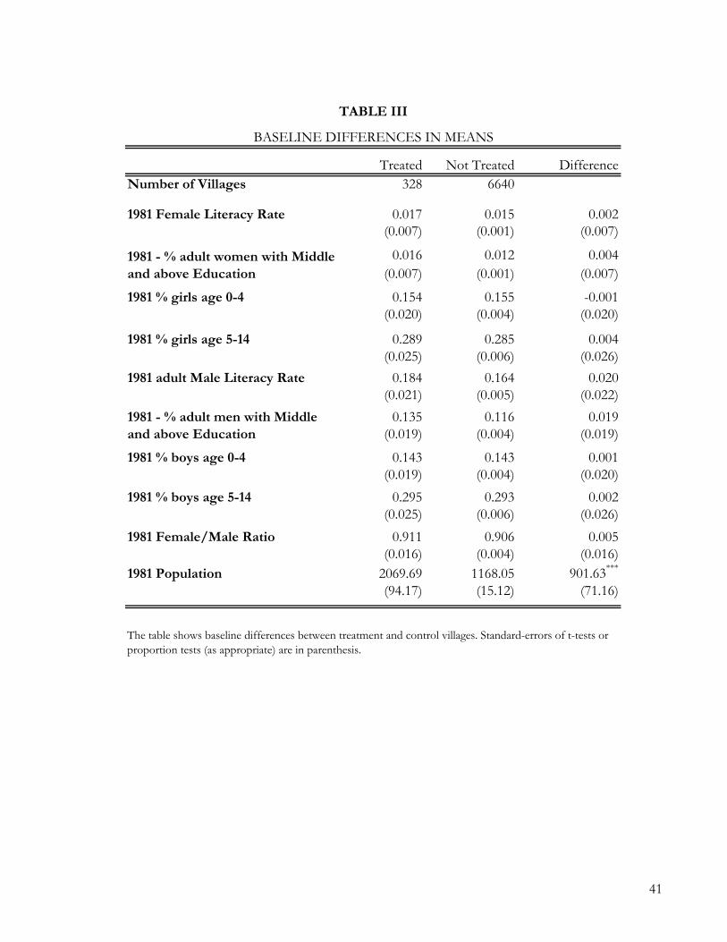
Treated Not Treated DifferenceNumber of Villages 328 6640

1981 Female Literacy Rate 0.017 0.015 0.002(0.007) (0.001) (0.007)

0.016 0.012 0.004(0.007) (0.001) (0.007)

1981 % girls age 0-4 0.154 0.155 -0.001(0.020) (0.004) (0.020)

1981 % girls age 5-14 0.289 0.285 0.004(0.025) (0.006) (0.026)

1981 adult Male Literacy Rate 0.184 0.164 0.020(0.021) (0.005) (0.022)

0.135 0.116 0.019(0.019) (0.004) (0.019)

1981 % boys age 0-4 0.143 0.143 0.001(0.019) (0.004) (0.020)

1981 % boys age 5-14 0.295 0.293 0.002(0.025) (0.006) (0.026)

1981 Female/Male Ratio 0.911 0.906 0.005(0.016) (0.004) (0.016)

1981 Population 2069.69 1168.05 901.63***

(94.17) (15.12) (71.16)

The table shows baseline differences between treatment and control villages. Standard-errors of t-tests or proportion tests (as appropriate) are in parenthesis.

1981 - % adult men with Middle and above Education

1981 - % adult women with Middle and above Education

TABLE III

BASELINE DIFFERENCES IN MEANS

41

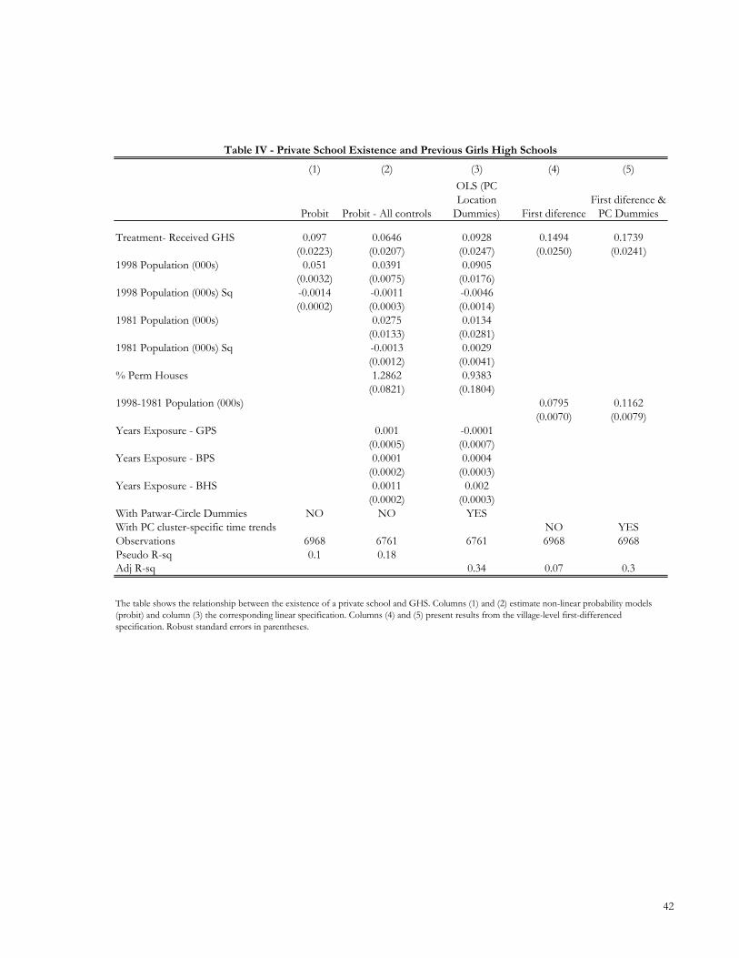
(1) (2) (3) (4) (5)

Probit Probit - All controls

OLS (PC Location

Dummies) First diferenceFirst diference &

PC Dummies

Treatment- Received GHS 0.097 0.0646 0.0928 0.1494 0.1739(0.0223) (0.0207) (0.0247) (0.0250) (0.0241)

1998 Population (000s) 0.051 0.0391 0.0905(0.0032) (0.0075) (0.0176)

1998 Population (000s) Sq -0.0014 -0.0011 -0.0046(0.0002) (0.0003) (0.0014)

1981 Population (000s) 0.0275 0.0134(0.0133) (0.0281)

1981 Population (000s) Sq -0.0013 0.0029(0.0012) (0.0041)

% Perm Houses 1.2862 0.9383(0.0821) (0.1804)

1998-1981 Population (000s) 0.0795 0.1162(0.0070) (0.0079)

Years Exposure - GPS 0.001 -0.0001(0.0005) (0.0007)

Years Exposure - BPS 0.0001 0.0004(0.0002) (0.0003)

Years Exposure - BHS 0.0011 0.002(0.0002) (0.0003)

With Patwar-Circle Dummies NO NO YESWith PC cluster-specific time trends NO YESObservations 6968 6761 6761 6968 6968Pseudo R-sq 0.1 0.18Adj R-sq 0.34 0.07 0.3

Table IV - Private School Existence and Previous Girls High Schools

The table shows the relationship between the existence of a private school and GHS. Columns (1) and (2) estimate non-linear probability models (probit) and column (3) the corresponding linear specification. Columns (4) and (5) present results from the village-level first-differenced specification. Robust standard errors in parentheses.

42

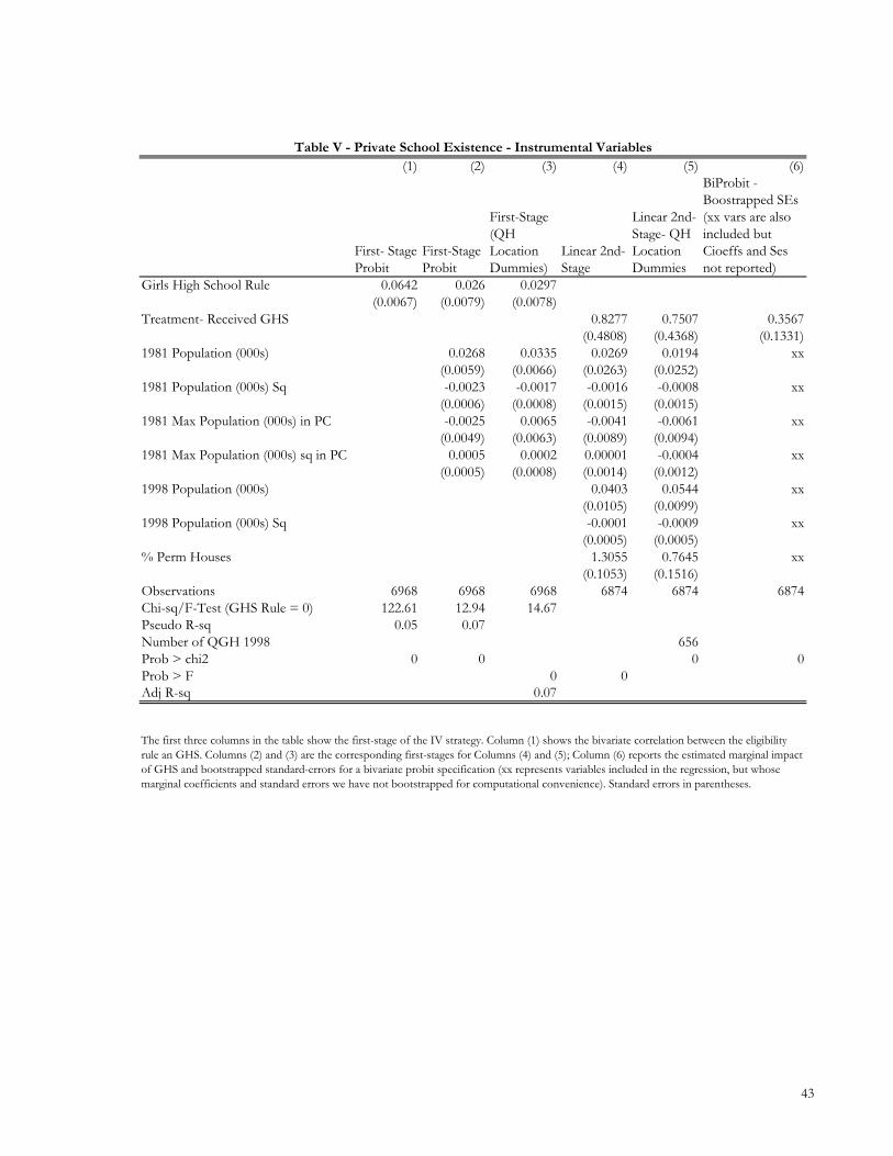
(1) (2) (3) (4) (5) (6)

First- Stage Probit

First-Stage Probit

First-Stage (QH Location Dummies)

Linear 2nd-Stage

Linear 2nd-Stage- QH Location Dummies

BiProbit - Boostrapped SEs (xx vars are also included but Cioeffs and Ses not reported)

Girls High School Rule 0.0642 0.026 0.0297(0.0067) (0.0079) (0.0078)

Treatment- Received GHS 0.8277 0.7507 0.3567(0.4808) (0.4368) (0.1331)

1981 Population (000s) 0.0268 0.0335 0.0269 0.0194 xx(0.0059) (0.0066) (0.0263) (0.0252)

1981 Population (000s) Sq -0.0023 -0.0017 -0.0016 -0.0008 xx(0.0006) (0.0008) (0.0015) (0.0015)

1981 Max Population (000s) in PC -0.0025 0.0065 -0.0041 -0.0061 xx(0.0049) (0.0063) (0.0089) (0.0094)

1981 Max Population (000s) sq in PC 0.0005 0.0002 0.00001 -0.0004 xx(0.0005) (0.0008) (0.0014) (0.0012)

1998 Population (000s) 0.0403 0.0544 xx(0.0105) (0.0099)

1998 Population (000s) Sq -0.0001 -0.0009 xx(0.0005) (0.0005)

% Perm Houses 1.3055 0.7645 xx(0.1053) (0.1516)

Observations 6968 6968 6968 6874 6874 6874Chi-sq/F-Test (GHS Rule = 0) 122.61 12.94 14.67Pseudo R-sq 0.05 0.07Number of QGH 1998 656Prob > chi2 0 0 0 0Prob > F 0 0Adj R-sq 0.07

Table V - Private School Existence - Instrumental Variables

The first three columns in the table show the first-stage of the IV strategy. Column (1) shows the bivariate correlation between the eligibility rule an GHS. Columns (2) and (3) are the corresponding first-stages for Columns (4) and (5); Column (6) reports the estimated marginal impact of GHS and bootstrapped standard-errors for a bivariate probit specification (xx represents variables included in the regression, but whose marginal coefficients and standard errors we have not bootstrapped for computational convenience). Standard errors in parentheses.

43

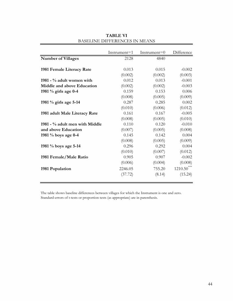
Instrument=1 Instrument=0 DifferenceNumber of Villages 2128 4840

1981 Female Literacy Rate 0.013 0.015 -0.002(0.002) (0.002) (0.003)

0.012 0.013 -0.001(0.002) (0.002) -0.003

1981 % girls age 0-4 0.159 0.153 0.006(0.008) (0.005) (0.009)

1981 % girls age 5-14 0.287 0.285 0.002(0.010) (0.006) (0.012)

1981 adult Male Literacy Rate 0.161 0.167 -0.005(0.008) (0.005) (0.010)

0.110 0.120 -0.010(0.007) (0.005) (0.008)

1981 % boys age 0-4 0.145 0.142 0.004(0.008) (0.005) (0.009)

1981 % boys age 5-14 0.296 0.292 0.004(0.010) (0.007) (0.012)

1981 Female/Male Ratio 0.905 0.907 -0.002(0.006) (0.004) (0.008)

1981 Population 2246.05 755.20 1210.50***

(37.72) (8.14) (15.24)

The table shows baseline differences between villages for which the Instrument is one and zero. Standard-errors of t-tests or proportion tests (as appropriate) are in parenthesis.

TABLE VIBASELINE DIFFERENCES IN MEANS

1981 - % adult women with Middle and above Education

1981 - % adult men with Middle and above Education

44

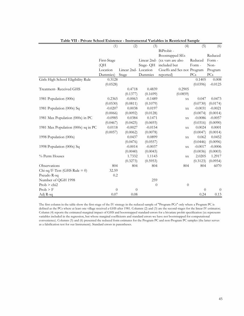
(1) (2) (3) (4) (5) (6)

First-Stage (QH Location Dummies)

Linear 2nd-Stage

Linear 2nd-Stage- QH Location Dummies

BiProbit - Boostrapped SEs (xx vars are also included but Cioeffs and Ses not reported)

Reduced Form - Program PCs

Reduced Form - Non-Program PCs

Girls High School Eligibility Rule 0.3128 0.1405 0.008(0.0528) (0.0396) -0.0125

Treatment- Received GHS 0.4718 0.4839 0.2905(0.1377) (0.1699) (0.0859)

1981 Population (000s) 0.2365 -0.0063 -0.1489 xx 0.047 0.0473(0.0530) (0.0811) (0.1079) (0.0730) (0.0174)

1981 Population (000s) Sq -0.0207 0.0038 0.0197 xx -0.0031 -0.0021(0.0066) (0.0092) (0.0128) (0.0074) (0.0014)

1981 Max Population (000s) in PC -0.0985 0.0384 0.1471 xx -0.0086 -0.0057(0.0467) (0.0425) (0.0693) (0.0316) (0.0090)

1981 Max Population (000s) sq in PC 0.0118 -0.0027 -0.0154 xx 0.0024 0.0001(0.0057) (0.0062) (0.0078) (0.0047) (0.0014)

1998 Population (000s) 0.0437 0.0899 xx 0.062 0.0452(0.0476) (0.0557) (0.0446) (0.0096)

1998 Population (000s) Sq -0.0014 -0.0037 xx -0.0017 -0.0006(0.0040) (0.0043) (0.0036) (0.0003)

% Perm Houses 1.7332 1.1143 xx 2.0205 1.2917(0.3273) (0.5953) (0.3123) (0.0954)

Observations 804 804 804 804 804 6070Chi-sq/F-Test (GHS Rule = 0) 32.59Pseudo R-sq 0.2Number of QGH 1998 259Prob > chi2 0 0Prob > F 0 0 0 0Adj R-sq 0.07 0.08 0.24 0.13

Table VII - Private School Existence - Instrumental Variables in Restricted Sample

The first column in the table show the first-stage of the IV strategy in the reduced sample of "Program-PCs" only where a Program PC is defined as the PCs where at least one village received a GHS after 1981. Columns (2) and (3) are the second-stages for the linear IV estimator; Column (4) reports the estimated marginal impact of GHS and bootstrapped standard-errors for a bivariate probit specification (xx represents variables included in the regression, but whose marginal coefficients and standard errors we have not bootstrapped for computational convenience). Columns (5) and (6) presented the reduced form estimates for the Program PC and non-Program PC samples (the latter serves as a falsification test for our Instrument). Standard errors in parentheses.

45

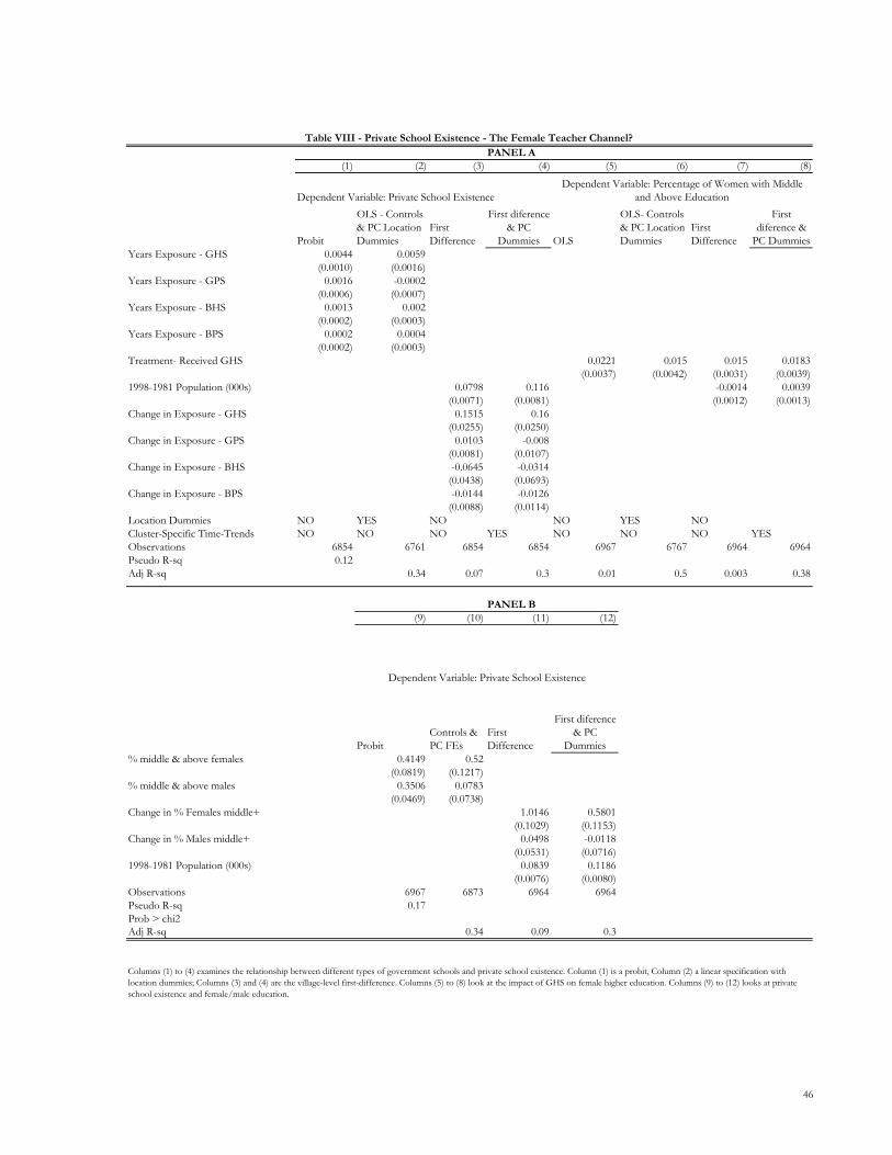
PANEL A(1) (2) (3) (4) (5) (6) (7) (8)

Dependent Variable: Private School Existence

Probit

OLS - Controls & PC Location Dummies

First Difference

First diference & PC

Dummies OLS

OLS- Controls & PC Location Dummies

First Difference

First diference &

PC DummiesYears Exposure - GHS 0.0044 0.0059

(0.0010) (0.0016)Years Exposure - GPS 0.0016 -0.0002

(0.0006) (0.0007)Years Exposure - BHS 0.0013 0.002

(0.0002) (0.0003)Years Exposure - BPS 0.0002 0.0004

(0.0002) (0.0003)Treatment- Received GHS 0.0221 0.015 0.015 0.0183

(0.0037) (0.0042) (0.0031) (0.0039)1998-1981 Population (000s) 0.0798 0.116 -0.0014 0.0039

(0.0071) (0.0081) (0.0012) (0.0013)Change in Exposure - GHS 0.1515 0.16

(0.0255) (0.0250)Change in Exposure - GPS 0.0103 -0.008

(0.0081) (0.0107)Change in Exposure - BHS -0.0645 -0.0314

(0.0438) (0.0693)Change in Exposure - BPS -0.0144 -0.0126

(0.0088) (0.0114)Location Dummies NO YES NO NO YES NOCluster-Specific Time-Trends NO NO NO YES NO NO NO YESObservations 6854 6761 6854 6854 6967 6767 6964 6964Pseudo R-sq 0.12Adj R-sq 0.34 0.07 0.3 0.01 0.5 0.003 0.38

PANEL B(9) (10) (11) (12)

ProbitControls & PC FEs

First Difference

First diference & PC

Dummies% middle & above females 0.4149 0.52

(0.0819) (0.1217)% middle & above males 0.3506 0.0783

(0.0469) (0.0738)Change in % Females middle+ 1.0146 0.5801

(0.1029) (0.1153)Change in % Males middle+ 0.0498 -0.0118

(0.0531) (0.0716)1998-1981 Population (000s) 0.0839 0.1186

(0.0076) (0.0080)Observations 6967 6873 6964 6964

Pseudo R-sq 0.17Prob > chi2Adj R-sq 0.34 0.09 0.3

Columns (1) to (4) examines the relationship between different types of government schools and private school existence. Column (1) is a probit, Column (2) a linear specification with location dummies; Columns (3) and (4) are the village-level first-difference. Columns (5) to (8) look at the impact of GHS on female higher education. Columns (9) to (12) looks at private school existence and female/male education.

Table VIII - Private School Existence - The Female Teacher Channel?

Dependent Variable: Percentage of Women with Middle and Above Education

Dependent Variable: Private School Existence

46

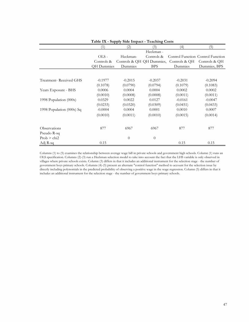
(1) (2) (3) (4) (5)

OLS - Controls &

QH Dummies

Heckman- Controls & QH

Dummies

Heckman - Controls &

QH Dummies, BPS

Control Function Controls & QH

Dummies

Control Function Controls & QH Dummies, BPS

Treatment- Received GHS -0.1977 -0.2015 -0.2037 -0.2031 -0.2094(0.1078) (0.0790) (0.0794) (0.1079) (0.1083)

Years Exposure - BHS 0.0006 0.0004 0.0004 0.0002 0.0002(0.0010) (0.0008) (0.0008) (0.0011) (0.0011)

1998 Population (000s) 0.0329 0.0022 0.0127 -0.0161 -0.0047(0.0233) (0.0320) (0.0309) (0.0451) (0.0433)

1998 Population (000s) Sq -0.0004 0.0004 0.0001 0.0010 0.0007(0.0010) (0.0011) (0.0010) (0.0015) (0.0014)

Observations 877 6967 6967 877 877Pseudo R-sqProb > chi2 0 0Adj R-sq 0.15 0.15 0.15

Table IX - Supply Side Impact - Teaching Costs

Columns (1) to (5) examines the relationship between average wage bill in private schools and government high schools. Column (1) runs an OLS specification. Columns (2)-(3) run a Heckman selection model to take into account the fact that the LHS variable is only observed in villages where private schools exists. Column (3) differs in that it includes an additional instrument for the selection stage - the number of government boys primary schools. Columns (4)-(5) present an alternate "control function" method to account for the selection issue by directly including polynomials in the predicted probability of observing a positive wage in the wage regression. Column (5) differs in that it includes an additional instrument for the selection stage - the number of government boys primary schools.

47

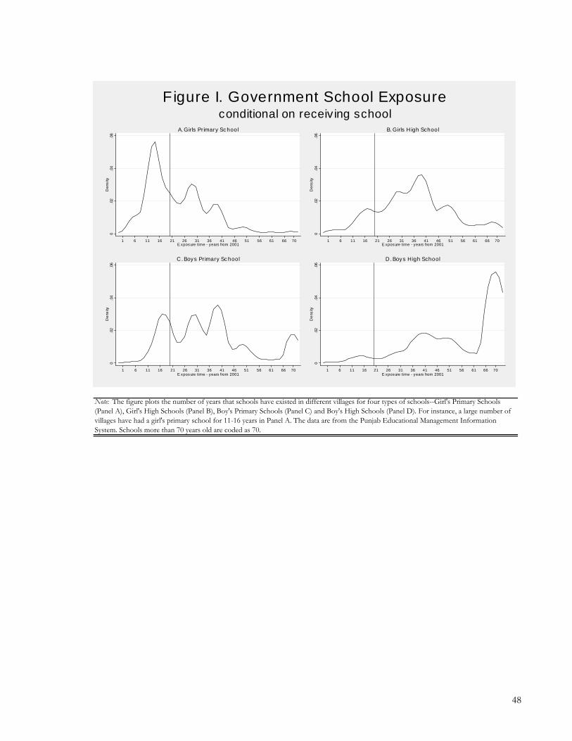
Note: The figure plots the number of years that schools have existed in different villages for four types of schools--Girl's Primary Schools (Panel A), Girl's High Schools (Panel B), Boy's Primary Schools (Panel C) and Boy's High Schools (Panel D). For instance, a large number of villages have had a girl's primary school for 11-16 years in Panel A. The data are from the Punjab Educational Management Information System. Schools more than 70 years old are coded as 70.

0.0

2.0

4.0

6D

ensi

ty

1 6 11 16 21 26 31 36 41 46 51 56 61 66 70E xposure time - years from 2001

A. Girls Primary Sc hool

0.0

2.0

4.0

6D

ensi

ty

1 6 11 16 21 26 31 36 41 46 51 56 61 66 70E xposure time - years from 2001

B. Girls H igh School

0.0

2.0

4.0

6D

ensi

ty

1 6 11 16 21 26 31 36 41 46 51 56 61 66 70E xposure time - years from 2001

C . Boys Primary Sc hool

0.0

2.0

4.0

6D

ensi

ty

1 6 11 16 21 26 31 36 41 46 51 56 61 66 70E xposure time - years from 2001

D . Boys H igh School

conditional on receiving schoolFigure I. Government School Exposure

48

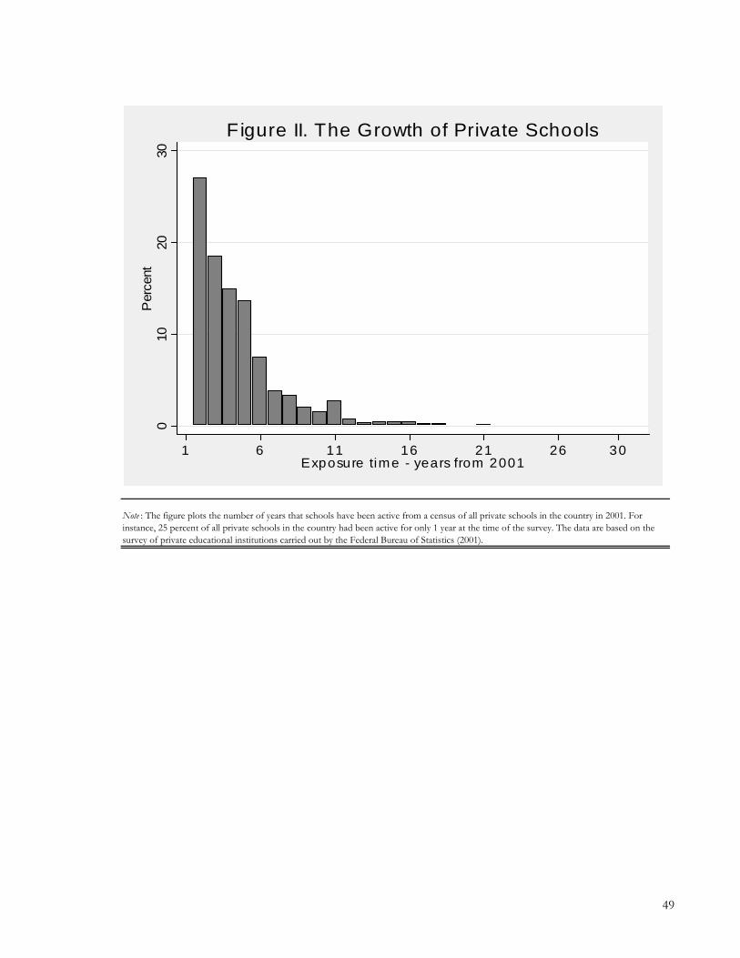
Note : The figure plots the number of years that schools have been active from a census of all private schools in the country in 2001. For instance, 25 percent of all private schools in the country had been active for only 1 year at the time of the survey. The data are based on the survey of private educational institutions carried out by the Federal Bureau of Statistics (2001).

010

2030

Per

cent

1 6 11 16 21 26 30Exposure time - years from 2001

Figure II. The Growth of Private Schools

49

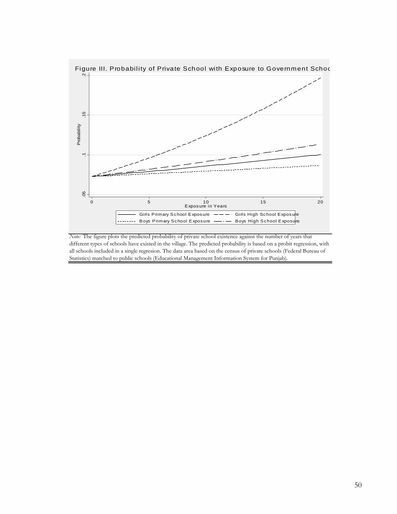
Note: The figure plots the predicted probability of private school existence against the number of years that different types of schools have existed in the village. The predicted probability is based on a probit regression, with all schools included in a single regresion. The data area based on the census of private schools (Federal Bureau of Statistics) matched to public schools (Educational Management Information System for Punjab).

.05

.1.1

5.2

Pro

babi

lity

0 5 10 15 20Expos ure in Years

Girls Primary Sc hool Expos ure Girls High Sc hool Expos ureBoys Primary School Exposure Boys High School Exposure

Figure III. Probabi l i ty of Priva te School wi th Exposure to Government Schoo

50

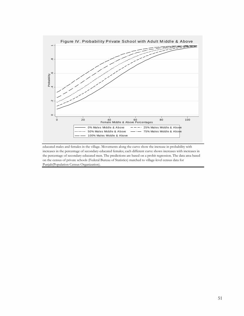
g p p p y p g p g yeducated males and females in the village. Movements along the curve show the increase in probability with increases in the percentage of secondary-educated females; each different curve shows increases with increases in the percentage of secondary-educated men. The predictions are based on a probit regression. The data area based on the census of private schools (Federal Bureau of Statistics) matched to village-level census data for Punjab(Population Census Organization).

0.2

.4.6

.81

Pro

babi

lity

0 20 40 60 80 100Female Middle & Above Percentages

0% Males Middle & Above 25% Males Middle & Above50% Males Middle & Above 75% Males Middle & Above100% Males Middle & Above

Figure IV. Probabi l i ty Private School wi th Adul t M idd le & Above

51

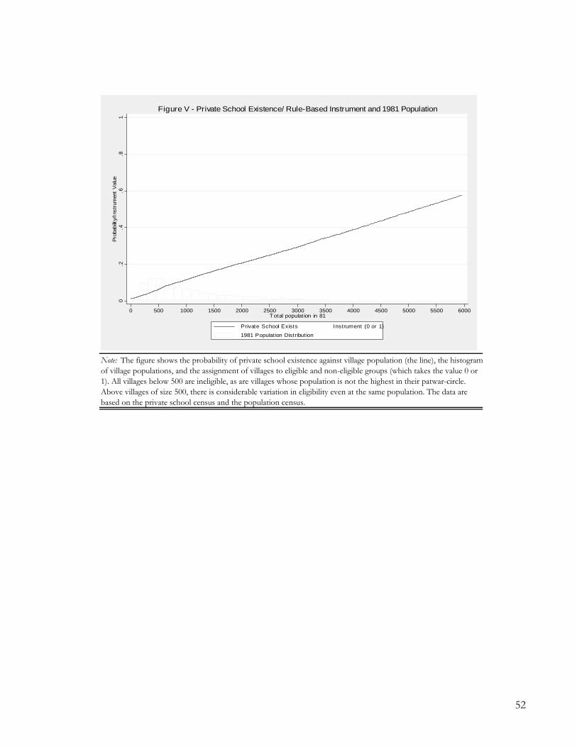
Note: The figure shows the probability of private school existence against village population (the line), the histogramof village populations, and the assignment of villages to eligible and non-eligible groups (which takes the value 0 or 1). All villages below 500 are ineligible, as are villages whose population is not the highest in their patwar-circle. Above villages of size 500, there is considerable variation in eligibility even at the same population. The data are based on the private school census and the population census.

0.2

.4.6

.81

Pro

babi

lity/

Inst

rum

ent

Val

ue

0 500 1000 1500 2000 2500 3000 3500 4000 4500 5000 5500 6000Total populat ion in 81

Private School Exists Instrument (0 or 1)

1981 Populat ion Distribution

Figure V - Private School Existence/ Rule-Based Instrument and 1981 Population

52

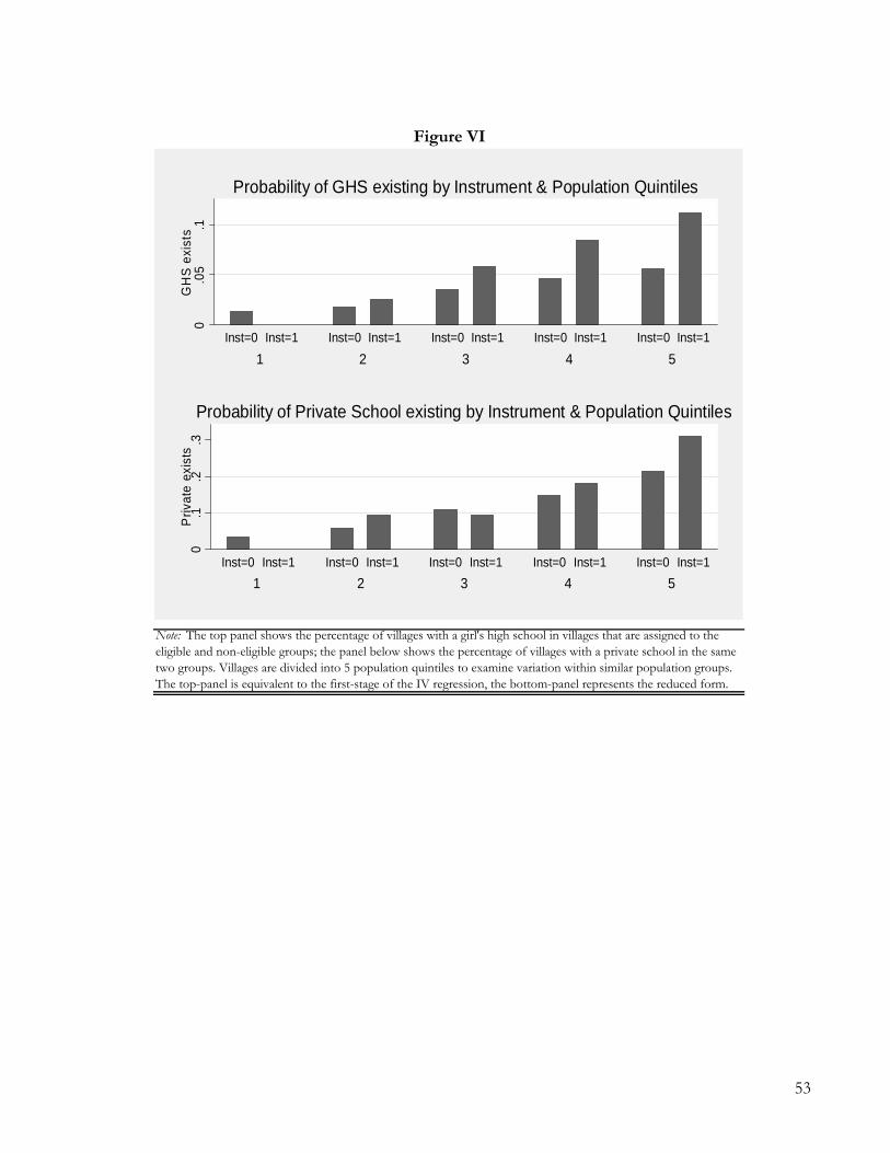
Note: The top panel shows the percentage of villages with a girl's high school in villages that are assigned to the eligible and non-eligible groups; the panel below shows the percentage of villages with a private school in the same two groups. Villages are divided into 5 population quintiles to examine variation within similar population groups. The top-panel is equivalent to the first-stage of the IV regression, the bottom-panel represents the reduced form.

Figure VI

0.0

5.1

GH

S e

xist

s

1 2 3 4 5Inst=0 Inst=1 Inst=0 Inst=1 Inst=0 Inst=1 Inst=0 Inst=1 Inst=0 Inst=1

Probability of GHS existing by Instrument & Population Quintiles0

.1.2

.3P

rivat

e ex

ists

1 2 3 4 5Inst=0 Inst=1 Inst=0 Inst=1 Inst=0 Inst=1 Inst=0 Inst=1 Inst=0 Inst=1

Probability of Private School existing by Instrument & Population Quintiles

53

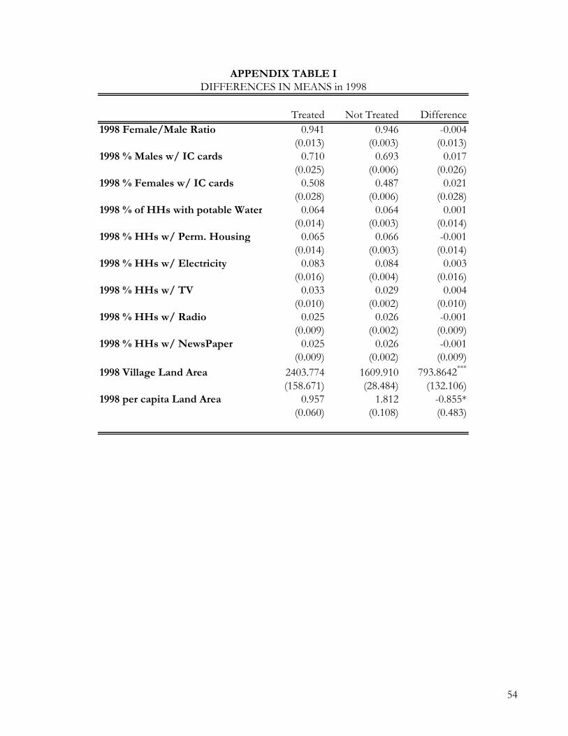
Treated Not Treated Difference1998 Female/Male Ratio 0.941 0.946 -0.004

(0.013) (0.003) (0.013)1998 % Males w/ IC cards 0.710 0.693 0.017

(0.025) (0.006) (0.026)1998 % Females w/ IC cards 0.508 0.487 0.021

(0.028) (0.006) (0.028)1998 % of HHs with potable Water 0.064 0.064 0.001

(0.014) (0.003) (0.014)1998 % HHs w/ Perm. Housing 0.065 0.066 -0.001

(0.014) (0.003) (0.014)1998 % HHs w/ Electricity 0.083 0.084 0.003

(0.016) (0.004) (0.016)1998 % HHs w/ TV 0.033 0.029 0.004

(0.010) (0.002) (0.010)1998 % HHs w/ Radio 0.025 0.026 -0.001

(0.009) (0.002) (0.009)1998 % HHs w/ NewsPaper 0.025 0.026 -0.001

(0.009) (0.002) (0.009)1998 Village Land Area 2403.774 1609.910 793.8642***

(158.671) (28.484) (132.106)1998 per capita Land Area 0.957 1.812 -0.855*

(0.060) (0.108) (0.483)

APPENDIX TABLE IDIFFERENCES IN MEANS in 1998

54