STUDIES IN CAPITAL BUDGETING - core.ac.uk · A Stochastic Model for the Growth Period Decision in 70. Forestry, Forthcoming in the Swedish Journal of Economics. 9. Optimal Capital

CARL J. NORSTR0M

STUDIES IN CAPITALBUDGETING

THE NORWEGIAN SCHOOL OF ECONOMICS AND

BUSINESS ADMINISTRATION

BERGEN 1975

c t_ \() 000

J... 'I.

PREFACE

In the preparation of the articles in this dissertation I have had

valuable commentsfrom several friends and colleagues. Someof my

gratitude is expressed in the individual articles. However, specialthanks must be given to Karl Borch, Jan Jvbssin and Agnar Sandrro.I will also use this opportunity to thank Leif Johansen -for encour-

agement and advice especially in connection with the last article in

the collection.

I am indebted to the Norway-AmericaAssociation and to the Norwegian

Research Council of Science and the Humanities for grants whichmade it possible to spend a year at the University of Michigan.

•

Finally I would like to thank the manysecretaries who typed thedifferent versions of these articles, especially Mrs. A. Hoem,

Mrs. E. Stiegler and Mrs. T. Hageselle .

•

CONTENTS

Pagel. A Modification of the Internal Rate of Return Method, l.

StatsØkonomisk Tidsskrift nr. 4, 1971, pp. 214-231.

2. A Mathematical Connection between the Present Value, 19.the Rate of Return and the Scale of an Investment,Journal of Business Finance,Vol. 4, No.2, 1972, pp.75-77.

3. Uniqueness of the Internal Rate of Return with Vari- 22.able Life of Investment: A Comment, Economic Journal,Vol. LXXX, December 1970, pp. 983-984.

4. A Sufficient Condition for a Unique Nonnegative Internal 24.Rate of Return, Journal of Financial and QuantitativeAnalysis, Vol VII, No.3, June 1972, pp. 1835-1839.

5. A Comment on Two Simple Decision Rules in Capital 29.Rationing, Forthcoming in the Journal of Business Financeand Accounting.

6. The Abandonment Decision under Uncertainty, Swedish 41.Journal of Economics, Vol. 72, 1970, pp. 124-129.

7. When to Drop a Produ9t: The Abandonment Decision under 47.Atomistic Competition, MarkedSkommunikasjon, Vol. 12,No.2, 1975, pp. 13-24.

8. A Stochastic Model for the Growth Period Decision in 70.Forestry, Forthcoming in the Swedish Journal of Economics.

9. Optimal Capital Adjustment under Uncertainty, Journal of 86.Economic Theory, Vol. 8, No.2, June 1974, pp. 139-148.

1.

A MODIFICATION OF THE INTERNALRATE OF RETURN METHOD*

By CARL J. NORSTR0M

l. Introduction.The internal rate of return method is one of the rnarn methods

used by economists for evaluating investments. Due to the pioneringwork of Joel Dean [5] and others, it has also gained a certain accept-ance in practice. During the last twenty years several distinguishedeconomists have attacked the internal rate of return and claimedthat it, in contrast to the present value method, will not always leadto correct decisions. The aim of this article is to clarify the reasonsfor the weaknessesof the internal rate of return method, and to suggesta modification of the method. The most serious limitation in ouranalysis will be that the discount rate is the same in each period.The most important characteristics of the internal rate of return

compared with the present value are thatl. The internal rate of return depends only on the cash flows of theprojects and not on the discount rate.2. The internal rate of return is independent of the size of the in-

vestment in the sense that it is unchanged if each element of thecash flow is multiplied by the same number.The present value has none of these properties. It is a function of

the discount rate and proportional to the scale of the investment.It is a consequence of this difference in character of the two measuresthat each is better than the other for some purposes. Thus the internalrate of return is very suitable if we want to know for which values ofthe discount rate a project is profitable, while the present value ismuch simpler to use in the choice between mutually exclusive projects.Moreover property 2 above indicates that the internal rate of returnis a better measure of the quality of an investment while the presentvalue also takes scale into consideration. We mention these pointsto indicate that establishing a correct version of the internal rate ofreturn method not only is a matter of academic interest, but has somepractical relevance as well.* The author is grateful to professor Jan Mossin for encouragement and advice.

Stats¢konc:misk 'I'i.dsskruf t nr. 4, 1971

2.

215

The main objections against the internal rate of return are thefollowing:l. The internal rate of return is not unique. There exist cash flows

with none as well as cash flows with more than one internal rateof return.

2. The internal rate of return method may lead to incorrect decisionsin the choice between mutually exclusive investments.

The readers interested in a more detailed discussion of these weak-nesses are referred to Lorie and Savage [13], Solomon [15], Hir-shleifer [7], Bailey [l], and Bernhard [2).1 These works have con-tributed to the understanding ot both the present value and internalrate of return method.

2. Assumptions and Definitions.The article is based on the following fundamental assumptions:l. Each project is fully described by a net cash flow, e. g.

(llo, at, ... , an), where a, is the net in- or outflow in period t.Each flow takes place at the end of the corresponding period.For convenience we shall assume flo *0.

2. In any period the firm may borrow or lend an arbitrary largeamount at a rate of interest, e. This rate will be referred to as thecost of capital. Unless otherwise stated it will be assumed thate ~O, but as will become clear this is not an essential assumption.

We shall make use. of the following definitions and notation:3. Some mathematical notation will be used in the usual way.

(a,b) denotes the open interval between a and b, and [a,b) thehalf-open interval. Note that if a=b, then (a,b) =[a,b) =O, theempty set. The union of two sets is denoted by U and the inter-section by n. 18 '1) denotes that 1 is an element in '1).

4. Since a project is fully described by the associated cash flow weshall not distinguish between the project and the cash flow butdenote both by a capital roman letter without subscript, e.g.A, B, C. Thus we have A=(flo, at> ... , an).

l Hirshleifer seems later to have modified his view. See Hirshleifer [9) for a morerecent statement of his opinion.

216

5. The cash flow A+B is defined by A+B=(tZo+bo, a1+b1, ... ,a,,+b,,). A -B is defined in a similar manner. Note that the cashflow resulting from accepting A and B is not necessarily A+B,since the cash flows may be dependent.

6. The present value function (of project A) is defined as

where i is a rate of interest.7. The present value, Pee), is the value of the present value function

when i=e.8. A number r is a root in the equation P(i) =0 if the equation holds

for i=r. r is a simple root if.P(i) =0 and P(i)j(i -r) *0 when i=r.r is a repeated root if P(i) =0 and P(i)j(i -r) =0 when i=r.

9. An internal rate of return r of the cash flow (tZo, al' ... , all) isa root of the equation

P(i)=tZo+alj(l+i)+ ... +all/(l+i)"=O.

It is customary also to restrict r to some set of numbers. We shalldenote this set 1). It is a natural choice to let 1)=[0, 00) andwe shall do so unless otherwise stated.

10. A cash flow (ao,al' ... , all) is said to have a unique internal rateof return if there exists one and only one r in 'l) such that r isa root in P( i) =0 and that moreover it is a simple root."

Il. In the discussion of one project, rl>r2, ••• will denote the differentrates of return of this project. When discussing ditferent projects,rA' rB etc. will denote rates of return of projects A, B etc. In thesame way PACe), PB(e) etc. will denote the present values of thedifferent projects.

I The restriction of T to be a simple root is made to make the internal rate of returnmethod more easily applicable. With this definition an investment project with aunique internal rate of return will have a positive present value if and only if theinternal rate of return is greater than the cost of capital. This is not necessarily thecase, when r is a repeated root. It is therefor unpractical to define uniqueness insuch a way that cash flows with one set of repeated roots are counted as cash flowswith a unique internal rate of return. See Bernhard [3] who criticizes the internalrate of return for this reason.

3.

4.

217

3. Independent Projects with Unique Internal Rates of Return.It is well known that the present value method and the internal

rate of return method will always lead to the same results in accept-reject decisions on independent projects with a unique internal rate ofreturn. This will be shown in this section in essentially the same wayas by Lorie and Savage [I3].

Multiplication with (1+i)" and substitution of x= 1-l-i transformthe equation P(i) =0 into the more suitable form

ffi) =a.,x"+atx"-l+ .. , +all=O.

Then i=x-l and the relevant range of values for x is [1,00). Thefollowing theorem is well known" from the theory of algebraic equa-tions:

Theorem 1. An odd number or an even number of real roots of anequationf(x) =0 lie between the two values x=a and x=b accordingasf(a),f(b) differ in sign or have the same sign.

We shall classify the cash flows with a unique internal rate of returninto two classes, according to the sign of flo.4 The fact that there is

•an odd number of roots in [1,00) implies that Ilo and L at never

n t..",O

will have the same sign, sincef(l)= L at andf(x) for large values1=1

of x have the same sign as ao• We define:l. Projects with a unique internal rate of return,

n

flo <o and L at ~O, are called simple investment projects.l-O

2. Projects with a unique internal rate of return,n

flo >Oand L at ~ O, are called simple financial projects.1=0

It follows from the theorem that a simple investment project hasa positive present value if the cost of capital fl is less than the internalrate of return r and a negative present value if fl is greater than r,Hence there is no conflict between the present value method and theinternal rate of return method in this case.

3 See e.g. Turnbull [17], page 95-96.4 We have for convenience assumed that Ilo * O. If Ilo = O for some cash flow,

it may be classified according to its first non-zero element.

218

The same line of argument holds for simple financial projects, butnow the present value is negative for e less than r and positive for egrater than r, These projects are accepted when the internal rate ofreturn is lower than the cost of capital.

Many writers have presented examples of cash flows with eithernone or multiple internal rates of return. However, the following suf-ficient condition shows that uniqueness holds for a large and importantclass of cash flows. Let At=ao+a1 + ... +a" i.e, the undiscountedaccumulation of the cash flow from O to t.

Theorem 2. A cash flow (ao, al' ... , an) with accumulated cash flow(Aø, Al! ... , All) will have a unique nonnegative internal rate of returnif the accumulated cash flow changes sign once and AII"* O.

A proof of this theorem is given in Norstrøm [14].The above theorem gives sufficient but not necessary conditions

for a unique internal rate of return. A general procedure for finding thenumber of roots ofj(x) =0 in any interval was found by the Frenchmathematician Sturm in 1829 and is known as Sturm's Theorem.!

4. Dependent Projects.Two projects A and B are dependent if the cash flow resulting from

accepting them both is different from the sum of the cash flows ofeach separate project. The type of dependence mostly discussed incapital budgeting is the case where the projects are mutually exclusive,i.e. when only one of the projects in question may be chosen. This caseis important since any decision concerning acceptance of projects -dependent or independent - may be seen as the choice betweenmutually exclusive projects - or sets of projects. If e.g. the projectsA and B are dependent, but not mutually exclusive, the decision maybe seen as the choise between: A and B; A; B; neither A nor B.Furthermore the choice between many mutually exclusive projectsmay be seen as a sequence of choice between pairs of mutually ex-clusive projects. It follows that it will be sufficient to give a treatment

5 For a statement and proof of Sturm's theorem see e.g. Turnbull [17J. Theapplication of Sturm's theorem to determine whether a cash flow has a uniqueinternal rate of return has been done by Kaplan [12J. Hf(x) = Ohas repeated roots,they are counted as one in Sturm's theorem. See Bernhard [3J and Turnbull [17].

5.

6.

219

of the choice between two mutually exclusive projects, since then inprinciple all cases are considered.

Formally the different investment methods may be said to consist ofl. A function which transforms the cash flow (and eventual para-

meters like the discount rate) into a measure of merit.2. Rules for using this function and the measure of merit. These may

include guidelines on which cash flows should enter into the func-tion and how the measure of merit should be used to reach adecision.There has been some disagreement on whether the internal rate of

return method will yield the same decisions as the present valuemethod in the choice between two mutually exclusive investments.This disagreement is due to diff~rent definitions of what the internalrate of return method is in this case, or more precisely - a differentopinion concerning the guidelines in 2. above. A specific examplewill clarify the point.

A company with cost of capital e=O.IO has the choice betweenthe two mutually exclusive A and B with cash flows A=(-200, 264),B=(-IOO, 143).

With the above cost of capital we havePACe) =40; TÅ=0.32PB(e) =30; TB=0.43

The most obvious way to use the internal rates of return is to choosethe project with the highest internal rate of return. If this is the guide-line for using the internal rate of return method for this case, thenclearly we have presented an example showing that the present valuemethod and the internal rate of return method may lead to differentdecisions."

• This version of the internal rate of return method has been criticized by e.g.Bernhard [2] and Hirshleifer [7]. It is easy to demonstrate that it leads to in-consistent results. Let C be another project, independent of A and B, and with cashflow C = (- 100, + 115). Since r = 0.15 is greater than the cost of capital,C is accepted. But B and C together has a cash flow B + C = (- 200, 258) whichclearly is inferior to A since Ilo = bo + Co and al > bl + Cl. To accept B and Ccan not be optimal since there exists an alternative which is better. (Whether thereexists still better alternatives is irrelevant.) Hence it has been demonstrated thatthis version of the internal rate of return method may lead to non-optimal decisions.

220

The advocates of the internal rate of return method do not, however,follow this procedure when choosing between two mutually exclusiveprojects." They regard the marginal cash flow A-B to be the relevantcash flow in this situation. Cash flow A is preferred to cash flow B ifand only if the marginal cash flow is preferred to nothing. Given thatthe decision on the marginal cash flow is in accordance with the presentvalue method, this will lead to a correct choice between A and B,because PÅ-B(e) >0 if and only it PÅ(e) >PB(e). In the above examplethe marginal project is A-B = (-100, +121). The internal rate ofreturn rÅ_B=0.21 is greater than the cost of capital e and hence projectA is chosen, which is in accordance with the present value method.Note that the decision is not influenced of whether A-B or B-Ais regarded as the marginal cash flow, since B-A will be rejectedif and only if A-B is accepted.

Essentially the same argument holds when the cash flow in questionmay be continuously varied through the choice of some input variables.We shall as an illustration consider the case that the cash flow at time tis a continuously differentiable function of a single variable Å; a,(Å).The optimization problem consists in choosing an optimal value for Å.Let a,'(A.) denote the derivative of a,(Å) with respect to Å. The marginalcash flow is then (llo'(Å), at'(Å), ... , an'(Å)), and the first order condi-tion for optimum according to the marginal version of the internalrate of return method is that an internal rate of return of this cashflow should be equal to the cost of capital e. But this is exactly the samefirst order condition as obtained when using the present value method,SInce

dP d {n a'(Å)} n a,'(Å)dA. = ri). l~o(l+e)1 = l~o(l+e)1 = 0,

which implies that e is an internal rate of return of the marginal cashflow.

The marginal use of the internal rate of return in principie reducesthe choice between two mutually exclusive projects to an accept-reject decision of an independent project. It has previousiy been shownthat the present value method and the internal rate of return method

1 See e. g. Grant and Ireson [6] which is a standard textbook in the field.

7.

8.

221

will give the same decision in such cases if the internal rate of returnis unique. It remains to consider the case of non-uniqueness. When wein the following discuss a project, it is either an independent one orthe marginal cash flow between two mutuallyexclusive projects.

5. Multiple Internal Rates of Return.In section 3 a theorem was stated which shows that it is only in ex-

ceptional cases that a project will have none or more than one internalrate of return. It can not be denied, however, that such cases may oc-cur, especially as marginal cash flows, and the issue of non-uniquenessis undoubtly the most serious theoretical objection against the internalrate of return method.

The perhaps most famous example of a project with multiple ratesof return is due to Lorie and Savage [13] and Solomon [15]. Theproject considered is the installation of a larger oil pump that wouldget a fixed amount of oil out of the ground more rapidly than theexisting pump. The marginal cash flow resulting from installation ofthe larger pump is (-1,600, +10,000, -10,000). This cash flow hastwo rates of return; Tl=0.25 and T2=4.00.

Examples of cash flows with more than two internal rates of returnare also easily constructed. The cash flow (-l, +6, -Il, +6) hasthree rates of return; Tl=0.00, T2=1.00 and T3=2.00. Furthermore,some cash flows have no internal rate of return, e.g., (-l, 3, -2.5).(The two last examples are due to Hirshleifer [7].)The natural question to ask is now, which of the internal rates

of return is the relevant one. If in the pump example the cost of capitale=0.50, should the larger pump be rejected because Tl<e or acceptedbecause e <T2? It has been argued by many writers that the internalrate of return method breaks down in this case." One of the best knowncritics is Solomon [15] who answers the above question by saying:"The answer is that neither of these rates of return is a measure ofinvestment worth, neither has relevance to the profitability of theproject under consideration, and neither, therefore, is correct.v"

8 See e.g. Lorie and Savage [13], Solomon [IS], Hirshleifer [7], and Bernhard [2].9 Solomon [15], page 128.

222

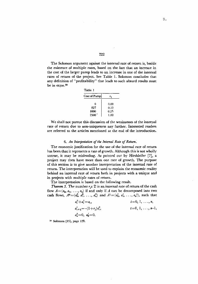
The Solomon argument against the internal rate of return is, besidethe existence of multiple rates, based on the fact that an increase inthe cost of the larger pump leads to an increase in one of the internalrates of return of the project. See Table 1. Solomon concludes thatany definition of "profitability" that leads to such absurd results mustbe in error. 10

Table I

Cost of Pumpl Tl

o 0.00827 0.101600 0.252500 - 1.00

We shall not pursue this discussion of the weaknesses of the internalrate of return due to non-uniqueness any further. Interested readersare referred to the articles mentioned at the end of the introduction.

6. An Interpretation of the Internal Rate of Return.The economic justification for the use of the internal rate of return

has been that it represents a rate of growth. Although this is not whollyuntrue, it may be misleading. As pointed out by Hirshleifer [7], aproject may then have more than one rate of growth. The purposeof this section is to give another interpretation of the internal rate ofreturn. The interpretation will be used to explain the economic realitybehind an internal rate of return both in projects with a unique andin projects with multiple rates of return.

The interpretation is based on the following result.Theorem3. The number Tie1) is an internal rate of return of the cash

flow A= (ao, al' ... , all) if and only if A can be decomposed into twocash flows, Ao=(ag, a?, ... , a~) and AI=(a~, al, ... , a,.l), such that

o la, +a,=a"

t=O, l, , n,

t=O, l, , n-l,a:+1=-(1 +Tj)a?,

a~=O, a~=O.

10 Solomon [15], page 128.

9.

10.

223

The proof of this theorem follows directly from the fact that a poly-nomialf(x) is divisible by (x-xi) if and only if Xi is a root inf(x) =0.

For example, the cash flow (-10, -15, +25, +30) has a uniquenon-negative internal rate of return, Tl=0.50. Using this rate of returthis cash flow is decomposed into the two cash flows, (-10, -30, -20,O) and (O, + 15, +45, +30).The important characteristic of the decomposition mentioned in

the theorem is that the cash flows AO and Al except for a shift of oneperiod have a similar development over time, so that it is meaningfulto compare the scale of the two cash flows. It is exactly the relativescale of the two cash flows which is measured through the internalrate of return. Nothing can be concluded from Tj about the profitabilityof the project before something is known about the cash flow AOand hence about AI. However, if A is regarded as an investment,a? may be interpreted to be the unrecovered investment at time t.llOne would then expect that like in the example a?;;; O for all t. Alarge positive internal rate of return will then mean high profitabilityas the cash flow Al will consist of positive elements and be large relativeto AO. Since for each t a~+1 is (l+Tj) times the absolute value of a?,but occurs one period later, the benefits of Al will dominate over thesacrifices of AO if and only if Tj > e. This is the well known rule fromsection 3 that an investment should be accepted if and only if itsinternal rate of return is greater than the cost of capital.

A similar line of argument holds for the case that a? ~ O and a: ;;;°for all t, conditions which usually hold for loans. Al will as abovedominate over AO if and only if Tj > e, but since AO now representsthe benefits and A1 the sacrifices, A should be accepted if and onlyif Ti <e.

The logic behind the above analysis is simple. The original cashflow is decomposed by use of the internal rate of return into two cashflows, in such a way that these are comparable, i.e. their relative sizemay be expressed as a number. A condition for this decompositionto be helpful is of course that it is easier to evaluate one of these cashflows than the original one.

In both cases considered ahove it was true that AO dominated overAl when Tl <e and Al over AO when Tl> (l. It is easy to see that this

11 See Bernhard (2).

224

holds generally since nothing in the argument depend of the natureof AO or AI, but only on the relation between them. A consequence ofthis is that from a decisionmaking point of view the only interestinginternal rates of return are those who lie in the range of possiblevalues of the cost of capital (l. For example, if it is known that the costof capital always will be non-negative, it will be of little interest todecompose a cash flow using a negative internal rate of return, sinceAO will dominate over Al with any possible value at e. The above argu-ment is to some extent an economic justification for the practice todisregard by definition negative internal rates of return.

As an example consider again the cash Howfrom the example abovewhich in addition to the internal rate of return rI =0.50 has two nega-tive ones, r2=-2.00 and ra=-3.00. Using ra the cash flow isdecomposed into' the two cash Haws, (-10, +5, +15, O) and(0, -20, + 10, +30). The decomposition achieves virtually nothingsince the critical information about the profitability of the project ishidden in the cash flows AO and Al and not contained in the internalrate of return. Further calculations are necessary to find for whichvalues of e the project is profitable.

As will be clear from the above discussion the explanatory powerof the decomposition is best when it is obvious which of the cash HawsAO and Al that represents the advantage and which the disadvantage.Two important classes of cash flows have this propertywhen de-composed.

The first of these consists of all cash flows which change sign once,from negative to positive, and with total receipts exceeding total out-lays. Such projects have been called conventional investments by somewriters.P It is well known that these cash flows have a unique non-negative internal rate of return, and it is easy to prove that when theyare decomposed we obtain cash flows AO and Al with a? ~O anda: ~ ° for all t. The cash flow in the example above belongs to thisclass.

The other class to be mentioned consists of projects with disposalcosts, such that there are net outlays in the beginning and the end ofthe project's life and receipts in the middle. It is still assumed that totalreceipts exceed total outlays. Such projects will have one internal rate

12 Bierman and Smidt [4].

11.

12.

225

of return in (-1,0) and one in (O,CXJ)_l3When the cash flows are de-composed, AO will contain positive as well as negative elements, butthe accumulated cash flow consisting of the elements A? = ag + a? +... + a? will be negative or zero for all t. It is easily seen from thisthat AO will be a clear disadvantage for all e ~O. An example of sucha cash flow is (-100, +110, +72, -18), with internal rates ofreturn Tl =-0.80 and T2=0.50. Using T2 it is decomposed into(-100, -;40, + 12, O) and (0, + 150, +60, -18). AO contains onepositive element, but is a clear disadvantage. The project should beaccepted if and only if T2 > e.

We shall now use the decomposition on projects with multipleinternal rates of return. Let A be a project with exactly two rates,Tl and T2• A can be decomposed using either of these rates. The ratenot used in the decomposition will be a unique internal rate of returnin AO and in AI. Two cases are "now possible depending on the signof ao: either AO is a simple investment project and Al a simple financialproject, or vice versa. We may conclude that any project with twointernal rates of return is a mixture of a simple investment and a simplefinancial project.

An example of a project with two internal rates of return is the oilpump project described in the previous section with the cash flow(-1,600, +10,000, -lO,UOO) and the two rates Tl=0.25 and T2=4.00.Using Tl this cash flow decomposed into (-1,600, +8,000, O) and(0, 2,000, -10.000).Note that noe only does the cash flow AO contain both negative and

positive elements, there is also a change in the accumulated cashflow. It is easy to prove that this always will be the case when theproject A has more than one positive internal rate of return. Henceit is no longer obvious whether a high internal rate of return indicateshigh or low profitability. The decomposition is still helpful, however,because it makes it possible to discuss projects with two internal ratesof return in terms of the more familiar projects with a unique one.

The case ao <O will be considered first. Let Tl and T2 be numbered

13 The fact that such cash flows have a unique internal rate of return has beenproved by Jean [10]. It does also follow as a corollary to Theorem 2 in section 3.It is necessary that total receipts exceed total outlays. See the discussion betweenHirshleifer [8] and Jean [11].

226

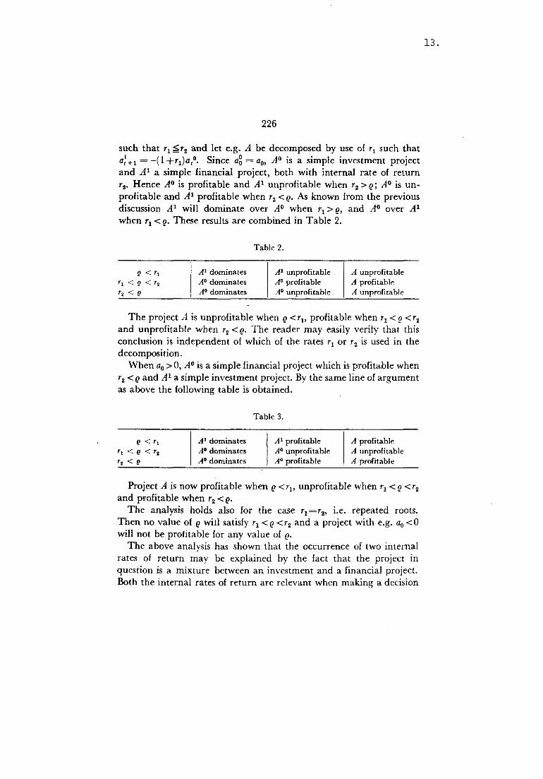
such that Tl ~T2 and let e.g. A be decomposed by use of Tl such thata: +1 = -(l +TI)a,o. Since ag = ao, AO is a simple investment projectand Al a simple financial project, both with internal rate of returnT2• Hence AO is profitable and Al unprofitable when T2 > e; AO is un-profitable and Al profitable when T2 < e. As known from the previousdiscussion Al will dominate over AO when Tl> e, and AO over Alwhen Tl <e. These results are combined in Table 2.

Table 2.

A unprofitableA profitableA unprofitable

Al dominatesAO dominatesAO dominates

Al unprofitableAO profitableAO unprofitable

The project A is unprofitable when e <Tl' profitable when Tl< e <T2

and unprofitable when T2 <e. The reader may easily verify that thisconclusion is independent of which of the rates Tl or T2 is used in thedecomposition.

When ao >0, AO is a simple financial project which is profitable whenT2 < e and Al a simple investment project. By the same line of argumentas above the following table is obtained.

Table 3.

A profitableA unprofitableA profitable

Al dominatesAO dominatesAO dominates

Al profitableAO unprofitableAO profitable

Project A is now profitable when e <Tl' unprofitable when rI <e <r2and profitable when T2 < e.

The analysis holds also for the case Tl=T2, i.e. repeated roots.Then no value of e wiil satisfy Tl < e < T2 and a project with e.g. ao < °will not be profitable for any value of e.The above analysis has shown that the occurrence of two internal

rates of return may be explained by the fact that the project inquestion is a mixture between an investment and a financial project.Both the internal rates of return are relevant when making a decision

13.

14.

227

on such a project.P Moreover, just as the unique internal rate of returndoes in a simple investment or financial project, these rates determinethe range of vaiues of the cost of capital which makes the projectprofitable.

The analysis could be extended to a discussion of projects with threeinternal rates of return in terms of projects with two rates and so on.In this way it is possible by economic arguments to obtain decisionrules for projects with any number of internal rates of return. Withthese decision rules it is possible to use the internal rate of returnmethod correctly. A different approach will be taken here. In the nextsection a measure of investment worth will be suggested, which may besaid to be another version of the internal rate of return, since it con-tains essentially the same information.

7. A Modification of the Internal Rate of Return Method.

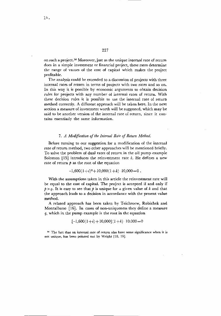
Before turning to our suggestion for a modification of the internalrate of return method, two other approaches will be mentioned briefly.To solve the problem of dual rates of return in the oil pump exampleSolomon [15] introduces the reinvestment rate k. He defines a newrate of return p as the root of the equation

-1,600(1 +i)2+ 10,000(1+k)-1O,OOO=O •

With the assumptions taken in this article the reinvestment rate willbe equal to the cost of capital. The project is accepted if and only ifp > (l. It is easy to see that p is unique for a given value of k and thatthe approach leads to a decision in accordance with the present valuemethod.

A related approach has been taken by Teichroew, Robichek andMontalbano [16]. In cases of non-uniqueness they define a measureq, which in the pump example is the root in the equation

[-1,600( 1+i) + 10,000](1 +k)-1O.000=0

14 The fact that an internal rate of return also have some significance when it isnot unique, has been pointed out by Wright [18, 19].

228

Teichroew, Robichek and Montalbano's approach contains toomany ideas to be given an adequate treatment here.P The importantpoints are again that q is unique for a given value of k, and that theapproach leads to the same decisions as the present value method.Both the approaches mentioned above represent moditications of

the internal rate of return method, which eliminates the problem ofnon-uniqueness of the internal rate of return. However, both have alsothe weakness that the rate p or q, which is used when a project hasmultiple rates of return is a function not of the cash flow alone, butalso of the reinvestment rate - or with our assumptions - the costof capital. This violates one of the fundamental characteristics of theinternal rate of return mentioned in the introduction, and makes themethod less useful when we want to know for which values of the costof capital a project is profitable ..It was mentioned in section 4 that the different investment methods

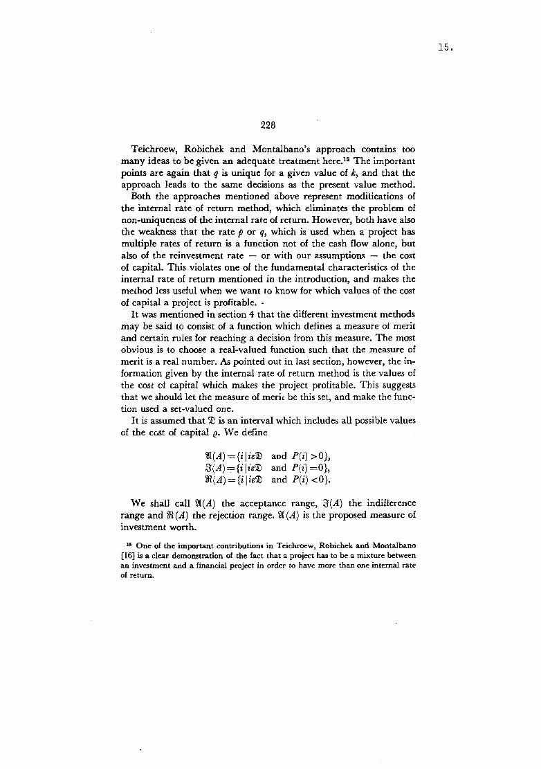
may be said to consist of a function which defines a measure ot meritand certain rules for reaching a decision from this measure. The mostobvious is to choose a real-valued function such that the measure ofmerit is a real number. As pointed out in last section, however, the in-formation given by the internal rate of return method is the values ofthe cost of capital which makes the project profitable. This suggeststhat we should let the measure of meric be this set, and make the func-tion used a set-valued one.It is assumed that '1) is an interval which includes all possible values

of the cost of capital e. We define

~(A) ={i lie'Il and P(i) >O},3(A) . {ilie'Il and P(i)=O},m(A)={ilie'Il and P(i) <O}.

We shall call ~(A) the acceptance range, 3(A) the indifferencerange and m (A) the rejection range. ~ (A) is the proposed measure ofinvestment worth.

16 One of the important contributions in Teichroew, Robichek and Montalbano[16] is a clear demonstration of the fact that a project has to be a mixture betweenan investment and a financial project in order to have more than one internal rateof return.

15.

16.

229

An independent project is accepted if and only if es~(A). The pro-ject is rejected if esffi(A) and one is indifferent with respect to theproject if e~(A).It is easy to see that the choice of the interval <1) has no influence

on the decision as long as <1) contains all possible values of the cost ofcapital. The choice of SDis therefore primarilyone of convenience.

Certain properties of the above sets are immediate.

(1)(2)(3)

~(A) U 3(A) U ffi(A) =SD,~(A) n 3(A) =~(A) n ffi(A) =3(A) n ffi(A) =O,

W(A) =ffi(-A), 3(A) =3(-A) •

(l) and (2) show that e is a number of one and only one of the threesets ~ (A), 3(~) and ffi (A), such that the decision rule lead to a uniquedecision.

In the choice between two mutually exclusive projects B and C,B is accepted if esW(B-C), C is accepted if (!sffi(B-C), and one isindifferent between B and C if e~(B-C). (3) assures that the decisionis not influenced by whether (B-C) or (C-B) is taken to be the mar-ginal project.

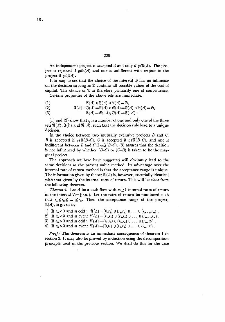
The approach we here have suggested will obviously lead to thesame decisions as the present value method. Its advantage over theinternal rate of return method is that the acceptance range is unique.The information given by the set W (A) is, however, essentially identicalwith that given by the internal rates of return. This will be clear fromthe following theorem.

Theorem 4. Let A be a cash flow with m ~ l internal rates of returnin the interval <1)=[0,00). Let the rates of return be numbered suchthat r1~ r:a~ ..• ~ rm' Then the acceptance range of the project,~(A), is given by

l) If llo<O and m odd: W(A)=[0,r1) U (r2,ra) u ... U (rm-l,rm).2) If llo<O and m even: W(A)=(rUr2) U (ra,r4) U ..• U (rm-l,rm) •3) If llo>O and m odd: ~(A)=(rl,r:a) U (ra,r4) U .•. U (rm, co) .4) If llo>O and m even: ~(A)=[O,rl) U (r:a,Ts)U .•• U (rm,oo).

Proof: The theorem is an immediate consequence of theorem l insection 3. It may also be proved by induction using the decompositionprinciple used in the previous section. We shall do this for the case

230

that m is odd and llo < O, i.e. case l. The proofs of the other cases aresimilar.

Decompose A into AO and Al using the internal rate of return T",.Since m is odd and llo <O, (m-l) will be even and og <O. Hence AOrepresents case 2 and Al case 4 in the theorem. By induction hypothesis&(AO)=(Tl,T2) U (T3,T.) U ... U (T",-2,T",-1) and 16(A1)=[0,T1) U (T2,T3) U••• U (r"':'1>OO). Al dominates in the interval [O,T",) and hence A willbe profitable in {&(Al) (l [0,T",)}=[0,T1) U (T2,T3) U ... U (T"'_l,T",). AOdominates in the interval (T""OO), but since T"'_l~T", AO and hence Awill be unprofitable in all of this interval. Combining the results provecase l.

We have in the theorem assumed that '!l=[0,(0). It is easily ex-tended to other choices of '!l. Note that & (A) is defined also whenthere is no internal rate of return. When '!l= [0,(0), & (A) =0 if Ilo <Oand &(A)='!l if 1lo>0.

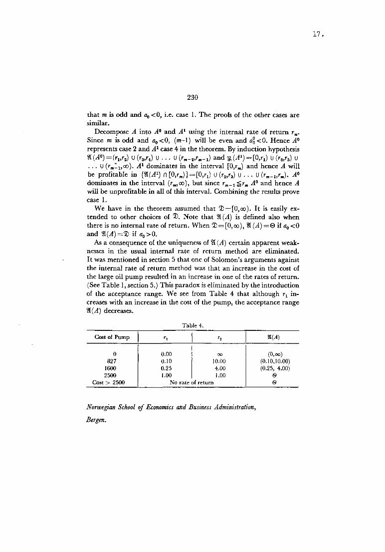
As a consequence of the uniqueness of & (A) certain apparent weak-nesses in the usual internal rate of return method are eliminated.It was mentioned in section 5 that one of Solomon's arguments againstthe internal rate of return method was that an increase in the cost ofthe large oil pump resulted in an increase in one of the rates of return.(See Table 1, section 5.) This paradox is eliminated by the introductionof the acceptance range. We see from Table 4 that although Tl in-creases with an increase in the cost of the pump, the acceptance range&(A) decreases.

Table 4.

Cost of Pump Tl '2 2t(A)

O 0.00 00 (0,00)827 0.10 10.00 (O.10, l 0.00)1600 0.25 4.00 (0.25, 4.00)2500 1.00 1.00 e

Cost> 2500 No rate of return e

Norwegian School of Economics and Business Administration,

BeTgen.

17.

18.

231

REFERENCES

[1] BAILEY, MARTIN J., "Formal Criteria for Investment Decisions." Journalof Political Economy, LXVII, No.6, October 1959.

[2] BERNHARD,RICHARD H., "Discount Methods for Expenditure Evaluation -A Clarification of Their Assumptions." The Journal of Industrial Engineering,Volume XIII, No.1, January-February 1962.

[3] Bernhard, Richard H., "On the Consistency of the Soper and Sturm-KaplanConditions for Uniqueness of the Rate of Return." The Journal of IndustrialEngineering, Volume XVIII, No.8, August 1967.

[4] BIERMAN,HAROLD, JR., and SEYMORSMIDT, The Capital Budgeting Decision.2nd Ed., Macmillan, 1966.

[5] DEAN, JOEL, Capital Budgeting. Columbia University Press, New York, 1951.[6) GRANT, EUGENE L., and W. GRANT IRESON,Principles of Engineering Economy.

4th Ed., The Ronald Press, New York, 1960.[7) HIRSHLEIFER,J., "On the Theory ~f Optimal Investment Decisions." Journal

of Political Economy, LXVI, No.5, August 1958.[8) HIRSHLEIFER,J., "On Multiple Rates of Return: Comment." Journal of Finance,

Vol. XXIV, No. l, March 1969.(9) HIRSHLEIFER,J., Investment, Interest and Capital. Prentice Hall Inc., Englewood

Cliffs, N.]., 1970.[10) JEAN, WILLIAMH., "On Multiple Rates of Return." Journal of Finance, Vol.

XXIII, No.1, March 1968.[11) JEAN, WILLIAMH., "Reply". Journal of Finance, Vol. XXIV, No.1, March

1969.[12) KAPLAN, SEYMOR,"A Note on a Method for Precisely Determining the Unique-

ness or Nonuniqueness of the Internal Rate of Return for a Proposed In-vestment." The Journal of Industrial Engineering, Volume 16, No. l, January-February 1965.

[13) LORIE, J. and SAVAGE,L. J., "Three Problems in Capital Rationing." Journalof Business, Vol. XXVIII, No.4, October 1955.

[14) NORSTR0M, CARL J., "A Sufficient Condition for a Unique Internal Rate ofReturn." Forthcoming in The Journal of Financial and Quantitative Ana~sis.

(15) SOLOMON,EZRA, "The ~ithmetic of Capital Budgeting Decisions." Journal ofBusiness, XXIX, No.2 April 1956.

[16) TEICROEW, D., ROBICHEK, A. A., and MONTALBANO,M., "An Analysis ofCriteria for Investment and Financing Decisions under Certainty." Manage-ment Science, Vol. 12, No.3, November 1965.

[17) TURNBULL,H. W., Theory of Equations. 5th. Ed., Oliver and Boyd, Edinburghand London, 1952.

(18) WRIGHT,J. F., "Notes on the Marginal Efficiency of Capital." Oxford EconomicPapers, Vol. XV, July 1963.

[19) WRIGHT, J. F., "Some Further Comments on the Ambiguity and Usefulnessof Marginal Efficiency as an Investment Criterion." Oxford Economic Papers,Vol. XVII, March 1965.

19.

A mathematical connection between thepresent value, the rate of return and thescale of an investmentby Carl J. NorstromAssistant Professor, Norwegian School of Economics and Business Administration,Bergen

AbstrfSGt: The purpose of this note is to show how discrepancies between the present values and rate of returns of investments aredue to differences in scale. A measure of the scale of a project is introduced and a mathematical connection between the presentvalue, rate of return and scale established.

THE two most important measures for evaluatinginvestments are the present value and the (internal)rate of return. It is well known that these measuresare not in complete correspondence: an investmentA may have a higher present value than investmentB, while B has a higher rate of return than A. l Abit imprecisely the reason for this may be said to bethat the rate of return measures only the quality ofthe investment, while the present value takes intoconsideration both the quality and the scale." Thepurpose of this note is to make this idea more preciseand show that it indeed is a correct one.

ONE-PERIOD INVESTMENTSIt is convenient first to discuss the simple case of

one period investments, where an amount is investedat time o and the benefits from the investment arereceived at time I, one period later. The cash flowfrom a project is of the form A= (ao, al), where for ausual investment ao<o and al>o. Let p denote themarket interest rate, and r the rate of return of thecash flow. The present value of the project is

V(A) = ao+-( al )'l+p

and the rate of return is given by

al0= ao+-(-)l+r

In the one-period case the investment outlay (- ao)is an obvious measure of the scale of the investment.

1 It is not an issue here whether the two measures lead todifferent decisions. A discussion of that question may be foundin eg, Bailey [I], Bernhard [2], Hirshleifer [4. 5], Lorie andSavage [6], Solomon [7] and Teichroew, Robichek andMontalbano [8].

2 See Bierman and Smidt [3], pp. 4O-.P.

Using (2) al may be eliminated from (I) byregular substitution. This gives

(r-p)V(A) = -( -) (-ao)

I+p

Equation (3) states that the present value of a pro-ject is equal to the difference between the rate ofreturn and the market interest rate, discounted oneperiod, times the scale of the project measured by theinvestment outlay. (3) makes, for the one-periodcase, explicit and precise how the present value takesinto account both the quality and the scale of a pro-ject, and explains why one project may have a largerrate of return than another and yet a smaller presentvalue.

MULTI-PERIOD INVESTMENTSThe ideas in the previous section will now be

generalized to multiperiod investments. The fol-lowing theorem will playa central part in the discus-sion:

Theorem. The number r is a rate of return of thecash flow A=(ao, all' .. , an)if and only if A can bedecomposed into two cash flowsAO-( o o O) d AI_( l l l)- ao, al'"'' an-l an - al' a2'"'' ansuch that

ag = ao

a?+ar = at t = 1,2, •.. , n- l

a! = ana1+1= (l+r)(-af) t = o, l, ... ,n-l (S)

The proof of the theorem follows directly from thefact that a polynomial/(x) is divisible by (x-a) ifand only if a is a root in the equation/(x)=o.We note that the first element of the cash flow AO

JOURNAL OF BUSINESS FINANCE. Vol. 4 No.2 © 1972 Mercury House Business Publications Ltd. 75

20.

Mathematical connection between present value, rate of return and scale of investment

refers to the present, while the first element in Altakes place at time L The cash flow AO plays a rolesimilar to ao in the one-period investments, and Alto al' (When n= I, AO=(ao) and AI=(al».The important characteristic of the decomposition

is that AO and Al have a similar development overtime. Mathematically they belong to a one-dimen-sional vectorspace, and it is therefore meaningful tocompare their relative size. It is exactly this relativesize which is reflected in the rate of return r.

An Example.It is easy to verify that the cash flow

A = (-1000, -1500, +2500, +3000)

has a rate ofreturn r=0·50. Decomposing A usingthis rate gives

AO = (- 1000, - 3000, - 2000)Al = (+1500, +4500, +3000)

The reader may verify that the decompositionsatisfies (4)- (5).

We want to find a measure of the scale of theinvestment which is an extension of the investmentoutlay (- ao), the measure in the one-period case. Itis easily seen that the cash flow A of the actualinvestment project is identical with the total cashflow resulting from n hypothetical, one-periodinvestments where the tth project takes place at timeI and has cash flow (ap, at + l)' The natural economic. . f AO (0 ° 0)' hmterpretation o = ao, ah ... , an _ l IS t ere-fore that (- ap) is the unrecovered investment attime t of the actual project." We shall measure thescale of the actual project by the present value of theunrecovered investments

n-l ( 0)V(-AO)- 2 ~

- t=o (I+p)t

It is now possible to derive a result for multiperiodinvestments, which is similar to (3) and include thisequation as a special case. It follows easily from (4)-(5) that the present value of the actual project is

V(A) = (r-p).V(_AO) (7)(I+p)

3 This interpretation is used in eg, Bernhard [2].

76

The economic interpretation of (7) is similar to thatof (3). The present value of a project is the product ofthe quality measured by (r-p) and the scalemeasured by (V( - AO», discounted one period.Eventual discrepancies between the present valuesand rates of return of two projects are the result ofdifferences in scale.

The economic interpretation of AO suggests thatap is negative and hence - ap positive, for all I. Itmay be proved that this will be the case for all cashflows A = (ao, ah' .. , an) with one change of signs.In this case it is obvious that V( - AO) is positive forall non-negative values of p, and that the informationof whether theproject has a positive present valueor not is contained in r. Although not so obviousfrom an economic point of view, the same is true forcash flows where some a? are positive as long as Ahas a unique rate of return and ao is negative.

The economic interpretation of a positive a? isthat the unrecovered investment is negative, or thatthe project at this point of time is a loan. It is wellknown that there exist projects with more than onerate of return. If such a cash flow is decomposedusing one of these rates, the remaining rates will alsobe rates of return in the cash flow AO. V( - AO) willthen be positive or negative according to the value ofp, reflecting the well known fact that projects withmultiple rates of return will act predominantly as aninvestment for some interest rates and as a loan forothers.

(6) REFERENCES[I] Bailey, Martin J., "Formal Criteria for Investment

Decisions", Journal of Political Economy, LXVII, No.6,October 1959.[2] Bernhard, Richard H., "Discount Methods for Expendi-

ture Evaluation-A Clarification ofTheir Assumptions", TheJournal of Industrial Engineering, Volume XII, No. I, January-February 1962.

[3] Bierman, Harold Jr. and Smidt, Seymor, The CapitalBudgeting Decision, 3rd ed., Macmillan, 1971.

[4] Hirshleifer, Jack, Investment, Interest and Capital,Prentice Hall, Inc., 1970.

[5] Hirshleifer, Jack, "On the Theory of Optimal Invest-ment Decisions", ]o_I of Political Economy,LXVI, NO.5,August 1958.[6] Lorie, James H., and Savage, Leonard J, "Three

Problems in Capital Rationing", Jo_I of Businm, Vol.XXVIII, No. 4. October 1955-

21.

[7] Solomon, Ezra, "The Arithmetic of Capital BudgetingDecisions",Jo_1 of Business,Vol. XXIX, No.2, April 1956.[8] Teichroew, Daniel, Robichek, Alexander A., and

Montalbano, Michal, "An Analysis of Criteria for Investmentand Financing Decisions under Certainty", ManagementScience, Vol. I2, NO.3, November 1965-

77

22.

1970] UNIQUENESS OF INTERNAL RATE OF RETURN: A COMMENT 983

UNIQUENESS OF THE INTERNAL RATE OF RETURNWITH VARIABLE LIFE OF INVESTMENT:

A COMMENT)

IN the article" Uniqueness of the Internal Rate ofReturn with VariableLife ofInvestment" published in the September 1969 issue of the ECONOMICJOURNAL,K.J. Arrow and D. Levhari consider the uniqueness of the internalrate of return when it is possible to truncate the investment project at anymoment of time. It has earlier been proved by Soper [3] and Karmel [2]that if the investor chooses the truncation period so as to maximise theinternal rate of return, then the truncated project has a unique internalrate of return. Arrow and Levhari point out that with a perfect capitalmarket the truncation period should be chosen so as to maximise the presentvalue of the truncated project and not its internal rate of return. Theythen go on to prove that if, with a given constant rate of discount, thetruncation period is chosen so as to maximise the present value of theproject, then the internal rate of return is unique.

The purpose of this comment is to demonstrate that the internal rate ofreturn Arrow and Levhari find, in reality, is Soper's maximal internal rateof return, i.e., the one that is obtained when the truncation period is chosento maximise the internal rate of return.

In correspondence with Arrow and Levhari's article let x(t) be a givencontinuous stream of net income and define

(l)

Thus t/>(r, T) is the present value of the stream x(t) when the discount rate isr and the truncation period T. Further, let

(2)

(3)

"'(r) = Max t/>(r, T)T

T(r)" = {Tlt/>(r, T) Max}

"'(r) is the maximum present value, for a given r, with the appropriate choiceof the truncation period, T; and T(r) is the set oftruncation periods leadingto the highest present value when the discount rate is r.

On the other hand, let T* be one of the truncation periods obtainedwhen the internal rate of return of the truncated project is maximised, andlet r* be the corresponding unique maximal internal rate of return.

In their article, Arrow and Levhari show that the maximum presentvalue "'(r) is a decreasing monotonic function of the discount rate r, andhence that there is at most one solution of "'(r) = O. This result is not

l The author wishes to acknowledge valuable comments by Professor K.J. Arrow on the fintversion of this note.

23.

984 THE ECONOMIC JOURNAL [DEC.

disputed.' What is claimed here is that the solution of t/J(r) = o (if sucha solution exists) is exactly Soper's maximal internal rate of return r*, i.e.,that t/J(r*) = O.

In the following it will be assumed that the net stream x(t) is negative insome interval before it turns positive for the first time, because otherwisethere will be no finite solution of the equation t/J(r) = O. This assumptionassures that for any truncation period T, (4)(r, T) is negative when r is largeenough.PItwill now be shown that tP(r*) = O. From the definition of r* and T*

it follows that 4>(r*, T*) = O. Let us show that 4>(r*, T*) = Max4>(r*, T).T

Suppose, to the contrary, that there exists a truncation period Tl such that4>(r*, Tl) > 4>(r*, T*) = O. Since 4>(r,Tl) by the assumption above will benegative when r is large enough, there exists an rI > r* such that 4>(rl' Tl)= O. But this is impossible, since r* is the largest possible internal rate ofreturn. Hence 4>(r*, T*) = Max 4>(r*, T). It follows that

T-(4) tP(r*) = Max4>(r*, T) = 4>(r*,T*) = O.

T

This concludes the proof.CARL J. NORSTRØM

. The Norwegian School ofEconomics and Business Administration.

REFERENCES

1. K. J. Arrow and D. Levhari, "Uniqueness of the Internal Rate of Returnwith Variable Life of Investment," ECONOMICJOURNAL, September 1969,pp. 560--6.

2. P. H. Karmel, "The Marginal Efficiency of Capital," with Appendix byB. C. Rennie, Economic Record, Vol. XXXV, No. 72 (1959),423-34.

3. C:S. Soper, " The Marginal Efficiency ofCapital: A Further Note," ECONOMICJOURNAL, March 1959, pp. 174-7.

1 Arrow and Levhari thus define the internal rate of return in the following way. Theycompute for any given rate of interest the optimal truncation period, and define the internal rateofreturn to be the rate ofinterest which, when the truncation period has been optimised with respectto it, yields a present value of zero.

2 Ifx(t) ;;i!: O,O.;; t .;; .,., and foTX(t)dt > Ofor some r > O, then for any finite r

.pCr) = Max 4>Cr, T) ;;i!: 4>Cr, .,.) > O.T

If, on the other hand, there exists a .,.> Osuch that x(t) .;; O,O .;; t .;; .,., and [XCt)dt <O,then for

anyfinite T and bounded functionx(t) therewill be an r such that l~(t)e-rtdt < O,since l~(t)rrtdtO T

approaches zero faster than [x(t)rrtdl when r approaches infinity.

24.

JOURNAL OF FINANCIAL AND QUANTITATIVE ANALYSISJune 1972

A SUFFICIENT CONDITION FOR A UNIQUENONNEGATIVE INTERNAL RATE OF RETURN

Cart J. NOl'stl'¢m*

1. IntroductionA proposition is proved which shows that each member of an important class

of investment and financing projects has a unique nonnegative internal rate ofreturn. Nonuniqueness of the internal rate of return is thus shown to occurless frequently than formerly believed. The correspondence between the proposi-tion and previous results on the uniqueness of the internal rate of return isbriefly indicated.

II. MethodOne of the problems in applying the internal rate of return in the evalua-

tion of investment projects is that it is not necessarily unique. This fact hasbeen noted by a number of writers, who have presented examples of cash flows witheither no or more than one rate of return.1 We shall here prove a sufficientcondition for uniqueness, which shows that the members of a large and importantclass of cash flows do have a unique rate of return.

Consider an inve8tment or financing project with cash flow fao' al' .,an}' An internal rate of return is usually defined as a rate of interest rhaving _the property that

(l) -n• + a (l+r) • O.n

thSince an ni order equation always will have n roots. real OT complex, therange of r has to be restricted if the question of uniqueness is to be meaning-ful. We shall restrict r to being a nonnegative real number. The cash flowfao' al' •• " an} is said to have a unique internal rate of return if there is

*Univel'sity of ~higan.

lSee, e.g., Wright [12]. Samuelson [8]. Lorie and Savage [6]. Solomon [9),and Hirsh1eifer (3).

1835

25.

one and only one r ~ O, such that (1) holds and moreover that this r is a simpleroot in (1).2

Multiplication with (l+r)n and substitution of xinto the more suitable form

l+r transforms (l)

(2) O .

Here r ..x-l and the relevant range of values for x is (l, 00). We define

(3) A ..t

At is the undiscounted accumulation of the cash flow from T ..O to T ..t. Themain result in this note is:

Proposition 1. A cash flow {a , al' •• o, a } with accumulated cash flowo n{Ao' ~, ••• , An} will have a unique" nonnegative internal rate of return ifthe accumulated cash flow changes signs once and A + O.

nProof. Since f(x) = O is equivalent to -f(x) O, it may be assumed with-

out loss of generality that A .. a < O and hence A > O. There is at least oneo o n

root of f(x) in (l, 00), since f(l) = A and f(x) will have the same sign as An o

~hen x is large enough. x = l is not a root since A # O.n

It remains to show that there is at most one root. Suppose that there ismore than one root and that these roots are numbered xl ~ x2 ~ •••• It will beshown that ~ > l and f(~) ..O implies that the derivative f'(~) < O. Thisimplies that xl is unique. f'(xl) < O implies in the first place that xl is asimple root and moreover that f(x) < O for xl < x < x2' but. then must -f'(x2) ~ O, which is a contradiction.

We have

(4) f(x) .. (x-l) (A xn-l + A n-2 A ) + Ao lX + ... + n-1 n'

Define

2The restriction of r to being a simple root in (l) is made to make theinternal rate more easily applicable. With this definition an investment projectwith a unique internal rate of return will have a positive present value ifand only if the internal rate of return is greater than the c'ilculation rate.This is not necessarily the case when r is a repeated root in (l). It is there-fore impractical to define uniqueness in such a way that cash flows with one setof repeated roots are counted as cash flows with a unique internal rate of return.See Bernhard. [2], who criticizes the internal rate of return for this reason.

1836

26.

(5) g(x) A n-l + A 0-2OX lX + ... + Ao_l

such that

(6) f(x) (x-l)g(x) + A , ando

(7) f' (x) (x-l)g'(x) + g(x).

suchLet ~ > ~.and f(~) = O. We shaH show that g(~) < O and g'(~) < O

that from (7) f'(~) < O. g(~) < O follows immediately from (6) andO. As there is only one change of signs in the accumulated cash flow,A >

nthere must be an integer m such that

A < Ot=

A > Ot-

for t = O, l, ..• , m, and

for t • m+l, ••.• n.

Hence,

(8) n-l n-mmAo~ + ... + Am_l~

- Am+l~-m-2 - ... - (n-m-l)An_l < O.

since all the coefficients are negative. Since n-m-l ~ O and g(~) < O, itfollows from (8) that gt(~) < O. Q.E.D.

The proposition g-ives sufficient but not necessary conditions for a uniqueinternal rate of return.3

We shall now briefly consider the correspondence between Proposition 1 andsome other results on the uniqueness of the internal rate of return.

Descartes Rule of Signs~ states that the number of positive roots in (2)cannot exceed the number of signs of the coefficients. Hence, there will be atmost ane internal rate of return if the cash flow {a , al' .•• , a } changeso nsigns once. The advantage of this result over Proposition 1 lies in that it isapplicable to interest rates r > -l (not only to r ~ O). When r is restrictedto being nonnegative, Descartes's Theorem obviously is less general.

3The cash flow {-l, 2, -2, 4} has a unique internal rate of return, r = 1.0,although the accumulated cash flow {-l, l, -l, 3} changes sign three times.

~See Turnbull [11], pages 99-102.

1837

27.

It follows as a corollary to Proposition l that an investment will have aunique nonnegative internal rate of return when there are two changes of signsin the original casle flow {a • al •••. , a } and moreover A = a and Ao n o o nao + al + . . . + an have different signs. This result is immediate when onenotices that the above conditions imply that the accumulated cash flow {Ao' Ar •• • " A } will change signs once and that A ~ O. The corollary is of some

n ninterest since it covers the case where there is an outlay at the end of aninvestment's life, due, e.g., to disposal costs. A slightly less general resultthan the corollary has previously been proved by J.ean [3].

The French mathematician Sturm found in 1829 a method for finding the exactnumber of distinct roots of (2) within any given range of values. Thus, Sturm'stheorem may be used to find for any given cash flow whether it has none. one, orsmany rates of return. The weakness of Sturm's theorem is that it is relativelycumbersome to apply and that it has no immediate economic interpretation.

Proposition 1 provides a convenieDt way of checking uniqueness, which maybe incorporated easily in computer programs calculating the internal rate ofreturn. Its economic significance lies in showing that the class of projectswith a unique internal rate of return is much larger than the class of projectswith one change of signs in the original cash flow. A project with nonuniqueinternal rates of return must have an accumulated cash flow which changes signsmore than once or not at all. This result is in accordance with the argumentsmade by Teichroew. Robichek. and Montalbano [10] and Bernhard [l] that a projecthas to be Il mixture of an investment and a loan in order not to have a uniqueinternal rate of return. Teichroew, Robichek, and Montalbano [10] have given anextended version of the internal rate of return method which yields the samedecisions as the present value method also for such projects.

REFERENCES

[1] Bernhard. R. H. "Discount Methods for Expenditure Evaluation - A Clarifica-tion of Their Assumptions." The JOW"Ylal of Indueiirial: Engineering, VolumeXII. No. I, January-February 1962.

[2] "On the Consistency of the Soper and Sturm-Kaplan Conditions forUniqueness of the Rate of Return." The JOUI"l1al of Indueta-ial: Engineering,Volume XVIII, No.8. August 1967.

[3] Hirshleifer. J. "On the Theory of Optimal Investment Decision." The JOUI"l1alof Political Economy, LXVI, No.5, August 1958.

[4] Jean, W. H. "On Multiple Rates of Return." The Journal of Finance, VolumeXXIII, No.1, March 1968.5For a statement and proof of Sturm's theorem see. e.g., Turnbull [11).

The a~plication of Sturm's theorem to determine whether a cash flow has a uniqueinternal rate of return has been done by Kaplan [5]. If f(x) has repeated roots,they are counted as one in Stunll's theorem. See Bernhard (2] and Turnbull [Il].

1838

28.

[5] Kaplan, S. "A Note on a Method for Precisely Determining the Uniqueness ofNonuniqueness of the Internal Rate of Return for a Proposed Investment."The Journal of Industrial Engineering~ Volume 16, No.1, January-February1965.

[6] Lori~, J. and L. J. Savage. "Three Problems in Capital Rationing." TheJGUPnal of Business. Volume XXVIII, No.4, October 1955.

(7] Norstrt!m, C. J. "Noen betraktninger om beregning og bruk av internrenten."Unpublished discussion paper, NHH, 1966.

[8] Samuelson, P. A. "Some Aspects of a Pure Theory of Capital." The QuarterlyJournal of Economics. Volume LI, May 1937.

[9J Solomon, E. "The Arithmetic of Capital Budgeting Decisions." Journal ofBusiness. Volume XXIX, No.2, April 1956.

[10] Teichroew, D.; A. A. Robichek; and M. Montalbano. "An Analysis of Criteriafor Investment and Financing Dec:i.sionsunder Certainty." Management Science.Volume 12, No.3, November 1965.

[111 Turnbull, H. W. ''Theory of Equations," 5th ed. Edinburgh: Oliver and Boyd.1952.

{12] Wright, C. A. "A Note on 'Time and Investment'." Baonomioa; New Series,Volume III, 1936.

1839

29.

Artikkelen .f.inneS

herA COMMENT ON TWO SIMPLE DECISION

RULES IN CAPITAL RATIONING*

uction

l rationing problem, optimal allocation of scarce

available investment projects, was introduced by

Savage in their famous article [5J. Weingartner [7J

~n elegant solution to the problem through the use

Jr integer programming. His contribution and later

y Baumol and Quandt [lJ, Myers [5J and others, have

panded the und~rstanding of the capital rationing

j related problems in finance. The application of

~h in real life situaticns is, however, severly

limited by the st~ong assumptions about the available

information; that the cash flows of all future projects up

to the planning horizon of the firm is known. This

requirement will not be satisfied in most real situations,

and the firm is left with the choice between more

conventional procedures, like the present value per dollar

outlay or the internal rate of return method.l The purpose

of this article is to give conditions under which these

simpler methods lead to essentially the same solution as

Weingartner' s linear pr-cgr-arnming approach. The condit ions

will be stated in terms of the shadow discount rates from

the linear programming solution.

l A similar view on this point has been expressed e.g. byHughes and Lewellen [4J.

* Fortheaningin the Journal of BusinessFinance and Accounting.Thecommentsof Karl Borch, SteinarEkern, Jan }bssin and Cary L. Sundernare gratefullyacknowledged.

30.

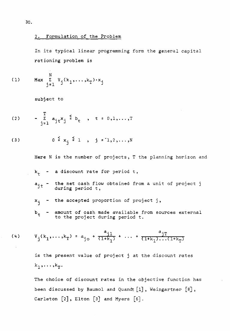
2. Formulation of the Problem

In its typical linear programming form the general capital

rationing problem is

N(l) Max I: V)' ( kl' ... ,kT)•x)'

j=l

subject to

t = O,l, ... ,T

( 3 ) o < x . < l)

Here N is the number of projects, T the planning horizon and

a discount rate for period t,

the net cash flow obtained from a unit of project]during period t,

the accepted proportion of project j,

amount of cash made available from sources externalto the project during period t.

(4) a,)0

+ ••• +a'T)

is the present value of project j at the discount rates

kl' ... ,kT·

The choice of discount rates in the objective function has

been discussed by Baumol and Quandt [lJ, Weingartner [SJ,

Carleton [2J, Elton [3J and Myers [6J,

31.

In the following we shall distinguish between current2(a. < O) and future investment projects (a. = O). It

JO JOis assumed that the cash flows of current projects are

known, but that the future projects, and a forteriori the

corresponding cash flows, are unknown. It follows that only

the current financial constraint (t = O in (2)) is known.

To distinguish this problem from the linear programming

problem (1)-(3), we shall call it Problem A.

We shall for convenlence make some simplifying assumptions.

It is assumed that the current financial constraint is

binding in the optimal sQlution of the primal problem

(1)-(3) as well as in the solutions obtained by the simpler

methods to be considered below. Otherwise there would not

be capital rationing in the usual sense. Moreover, we shall

assume that the optim~l solution of the problem (1)-(3) is

unlque and non-degenerate.

3. Analysis

The following result is an immediate consequence of the

duality theorems.

Proposition l. Assume that the primal problem (1)-(3) has a

unique, non-degenerate optimal solution. Then there exist

shadow interest rates Pl"" 'PT such that:

2 Deferment of projects lS not considered.

32.

(a) Any project which is fully accepted in the optimal

solution has a positive present value evaluated at

these interest rates.

(b) Any project which is partially accepted has present

value zero.

(c) Any project which is rejected has a negative present

value.

A firm which in addition to the cash flows of its current

projects knows the shadow interest rates Pl"" ,PT may

hence classify these projects into three classes.

Class l. Projects which ~n the optimal solution of the

primal problem (1)-(3) is fully accepted (x. = l).J

Class 2. Projects which are partially accepted (O < x. < l).J

Class 3. Projects which are rejected (x. = O).J

In general it is not possible on the basis of Pl"" ,PT and

the current financial restriction to determine the

proportion of each partially accepted project. Weingartner [7J

has shown that the optimal solution of the primal problem

(1)-(3) will include at most T partially accepted projects.

With a reasonable number of accepted projects in each period,

the relative number of partially accepted projects will be

small, and the classification above will be a good

approximation to the optimal solution of the primal.

33.

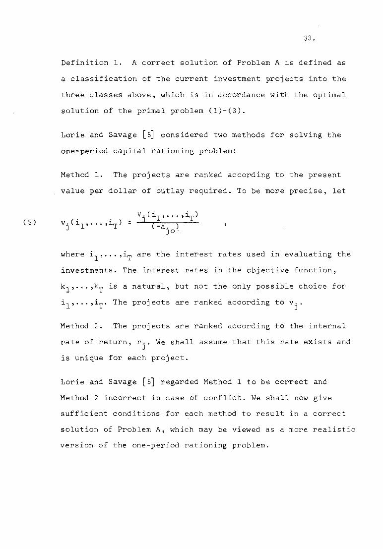
Definition l. A correct solution of Problem A is defined as

a classification of the current investment projects into the

three classes above, which is in accordance with the optimal

solution of the primal problem (1)-(3).

Lorie and Savage [~ considered two methods for solving the

one-period capital rationing problem:

Method l. The projects are ranked according to the present

value per dollar of outlay required. To be more precise, let

( 5 ) vj(il'...,iT )= Vj(il '...,iT)

(-a. )JO -

where il"" ,1T are the interest rates used in evaluating the

investments. The interest rates in the objective function,

kl"" ,kT is a natural, but not the only possible choice for

il"" ,iT' The projects are ranked according to vj.

Method 2. The projects are ranked according to the internal

rate of return, r .. We shall assume that this rate exists andJ

is unique for each project.

Lorie and Savage [5] regarded Method l to be correct and

Method 2 incorrect in case of conflict. We shall now glve

sufficient conditions for each method to result ln a correct

solution of Problem A, which may be viewed as a more realistic

version of the one-period rationing problem.

34.

Proposition 2. A sufficient3 condition for Method l, always

to give a correct solution of Problem A is that

Proposition 3. A sufficient3 condition for Method 2. always

to give a correct solution of Problem A is that

. .. -

Proofs of these propositions are given in the Appendix.

The sufficient conditions of the two problems are seen to be

of a different nature. Method l. will give a correct solution

to any problem as long as the firm is capable of estimating

the shadow prices of future periods. This estimation is likely

to be difficult, however, unless the capital rationing is of

temporary character. In particular Lorie and Savage's

conclusion is correct in the case they considered, capital

rationing in only the current period. The conditions of

Method 2. put restrictions on the problem itself. The method

is likely to give a good approximation to the optimal

solution if the investment and financing opportunities ln

the future are approximately as in the current period. If the

scarcity of capital is temporary, Method 2. will have a bias

in favor of projects with a short pay-back period.

3 The conditions are also necessary in the following sense.If the conditions are not satisfied, there will existproblems where Method l. (Method 2.) lead to an incorrectsolution. However, in a particulår problem either methodmay happen to result in a correct solution.

35.

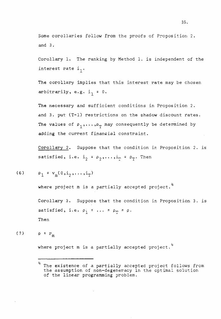
Some corollaries follow from the proofs of Proposition 2.

and 3.

Corollary l. The ranking by Method l. is independent of the

interest rate 11,

The corollary implies that this interest rate may be chosen

arbitrarily, e.g. il = O.

The necessary and sufficient conditions in Proposition 2.

and 3. put (T-l) restrictions on the shadow discount rates.

The values of Pl"" 'PT may consequently be determined by

adding the current finan~ial constraint.

Corollary 2. Suppose that the condition in Proposition 2. is

satisfied, i.e. i2 = P2,··· ,iT = PT' Then

where project m is a partially accepted project.4

Corollary 3. Suppose that the condition ln Proposition 3. is

satisfied, i.e. Pl = ••• = PT = p.

Then

where project m is a partially accepted project.4

4 The existence of a partially accepted project follows fromthe assumption of non-degeneracy in the optimal solutionof the linear programming problem.

36.

Corollary 2. provides in the application of Method l. a

possibility to check the realism of the discount rates

i2, ... ,iT' If the discount rate obtained from (6) e.g. is

much larger than i2, ... ,iT' this may indicate that these

rates are too low.

As seen above, Method l. and Method 2. both make implicit

assumptions on future shadow prices, which restrict these

rates to a one-dimensional curve in the T-dimensional space.

This order may be reversed, i.e., one may postulate a set of

conditions which restrict the shadow discount rates to a

one-dimensional curve, and then apply an iterative procedure

to select the investment projects. Whatever approach is taken

a record of past estimates of the shadow discount rates will

be valuable information in the firm's investment and

financial planning.

37.

Appendix

Proof of Proposition 2.

Sufficiency. Suppose that current project m belongs to

Class l. according to-the optimal solution of the linear

programming problem (1)-(3) and project n to Class 2. Then

and since for all current investment projects a. < O,JO

( 9 ) vm(Pl '...,PT) > vn(Pl '...,PT) .

It lS easily derived tha~ for any current project J

(10) ( )=-1+ l ( )vj Pl '...,PT (l+ Pl) wj P2'...,PT

where

(11 )l a'2= (--) [a. l + ]-a. J (1+P2)JO

+ ••• +

From (9) and (10) it follows that

and from (10) and (12) that

for all il > - l. Hence, if i2 = P2"" ,1T = PT' project mis ranked before project n by Method l. In a similar manner

it can be shown that project m is ranked before project n

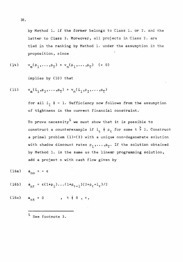
38.

by Method l. if the former belongs to Class l. or 2. and the

latter to Class 3. Moreover, all projects in Class 2. are

tied in the ranking by Method l. under the assumption in the

proposition, since

implies by (10) that

for all il + - l. Sufficiency now follows from the assumption

of tightness ln the current financial constraint.

To prove necessity5 we must show that it is possible to>construct a counterexample if lt t Pt for some t = 2. Construct

a primal problem (1)-(3) with a unique non-degenerate solution

with shadow discount rates Pl"" ,PT' If the solution obtained

by Method l. is the same as the linear programming solution,

add a project n with cash flow given by

( 16a) = - e:

( 16b) anl

( 16c) t to, l,

5 See footnote 3.

(17 )

(18)

39.

where T is smallest integer such that i 4 p and T ~ 2, andT TE > O is sufficiently small to preserve the basis in the

primal problem if project n lS accepted. Then project n is

classified in Class l. by the linear programming solution

and in Class 3. by Method l. if l > P , and vice versa ifT Ti < P • Q.E.D.T T

Proof of Proposition 3.

It has previously been assumed that each project has a

unlque internal rate of return. Suppose that project m belongs

to Class l. and project n to Class 2. according to the linear

programming solution and-that Pl = ... = PT = p. Then

V (p, ... ,p) > V (p, ... ,p) = Om n

(17) implies that

r > r = p.m n

The remaining part of the proof is similar the proof of

Proposition 2.

Proof of Corollary 2.

Suppose that project m is a partially accepted project.

From (10)

(20)

Substitution of the last equation in (20) into (19) gives (6).

40.

REFERENCES

l. W.J. Baumol and R.E. Quandt, "Investment and Discount RatesUnder Capital Rationing - A Programming Approach", TheEconomic Journal, LXXV (June 1965), pp. 317-329.

2. W.T. Carleton, "Linear Programming and Capital BudgetingModels", Journal of Finance, XXIV (December 1969),pp. 825-833.

3. E.J. Elton, "Capital Rationing and External Discount Rates",Journal of Finance, XXV (June 1970), pp. 573-584.

4. J.S. Hughes and W.G. Lewellen, "Programming Solutions toCapital Rationing Problems," Journal of Business Financeand Accounting, Vol. L (Spring 1974), pp. 55-74.

5. J.H. Lorie and L.J. Savage, "Three Problems in RationingCapital", Journal of Business, Vol. XXVIII (October 1955),pp. 229-239.

6. S.C. Myers, "A Note on Linear Programming and CapitalBudgeting", Journal of Finance, Vol. XXVII (March 1972),pp. 89-92.

7. H.M. Weingartner, "Mathematical Programming and the Analysisof Capital Budgeting Problems", Englewood Cliffs, N.J.Prentice Hall Inc. 1970.

8. H.M. Weingartner, "Criteria for Programming InvestmentProject Selection", Journal of Industrial Economics, Vol. XV(November 1966), pp. 65-76.

THE ABANDONMENT DECISION UNDERUNCERTAINTY

Carl J. Norstrem.The Norwegian School of Economics and Business Administration, Bergen, Norway

Summary

Two approaches to the abandonment problem under uncertainty are considered;the ECF-approach based on expected cash flows and the DP-approach using dy-namic programming. The ECF -approach is demonstrated to sometimes give incor-rect solutions. The DPcapproaoh is correct, but may be unfeasible due to the amountof numerical calculations. Under certain oonditions Markov programming may beused to obtain the correct solution. A general result on the connection betweenthe ECF-approach and the DP-approach is established.

l. One of the decisions in capital budgeting which has received special inter-est, is that concerning optimal replacement of equipment. A special case ofthis problem arises when it is assumed that the equipment will not be replaced,but that the production will come to an end when the equipment is sold. Thechoice of optimal time for abandoning production is easily solved under cer-tainty. In this article we shall consider some of the aspects of the abandon-ment problem under uncertainty.

2. It is assumed that the equipment in each period results in a net operatinginflow ZT which is realised at time T, the end of the period. The company con-siders in the end of each period whether production should halt and the equip-ment be sold for its abandonment value ST' If a decision is made not to sellthe equipment, production continues and the same question is consideredagain at the end of the next period. When the decision is made at time T, thefirm is assumed to know the net operating inflows and the abandonment val-ues up to that time, i.e. Zt and St for t ~T; as well as the conditional probabilitydistribution of Zt+l and St+1 for each t ~T,

(I)The objective of the firm is to maximize, at a given rate of discount r, the ex-pected present value of the total cash flow resulting from the equipment, andour problem is to find the abandonment time which achieves this.

3. One approach to finding the optimal abandonment time is to base the de-cision on the expected values for net operating inflows and abandonmentvalues. We shall call this the Expected Cash Flow approach, or for short the

Swed. J. of Economics 1970

41.

42.

Abandonment decision under uncertainty 125

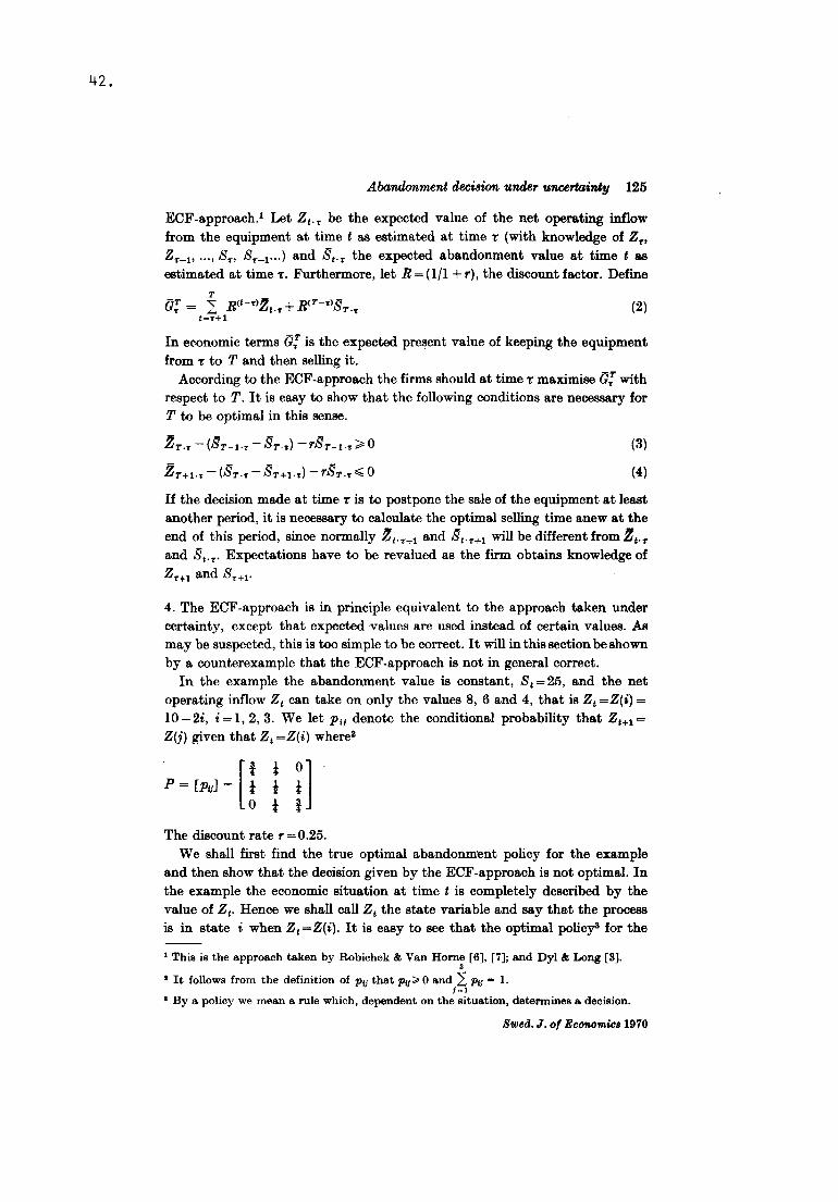
ECF-approach.l Let Zt.T be the expected value of the net operating inflowfrom the equipment at time t as estimated at time T (with knowledge of ZT'ZT_I' ... , ST> ST-l· ..) and SI.T the expected abandonment value at time t asestimated at time T. Furthermore, let R = (l/l + r), the discount factor. Define

TG; = 2: g.1-T)ZI.T+R<T-T)ST.Tt-T+I

(2)

In economic terms G; is the expected present value of keeping the equipmentfrom T to T and then selling it.

According to the ECF -approach the firms should at time T maximise G; withrespect to T. It is easy to show that the following conditions are necessary forT to be optimal in this sense.

ZT.T - (ST-I.T - ST.T) -rST-loT ~ O

ZT+loT - (ST.T - ST+I.T) - rSToT ~ O

(3)

(4)

If the decision made at time T is to postpone the sale of the equipment at leastanother period, it is necessary to calculate the optimal selling time anew at theend of this period, since normally ZtoHI and StOHl will be different from ZI.Tand StoT. Expectations have to be revalued as the firm obtains knowledge ofZHI and SHI·

4. The ECF-approach is in principle equivalent to the approach taken undercertainty, except that expected values are used instead of certain values. Asmay be suspected, this is too simple to be correct. It will in this section be shownby a counterexample that the ECF-approach is not in general correct.In the example the abandonment value is constant, SI=25, and the net

operating inflow ZI can take on only the values 8, 6 and 4, that is Zt =Z(i) =10 -2i, i=1,2,3. We let Pli denote the conditional probability that ZI+1=Z(j) given that Zt =Z(i) wheres

O [ip = [p,J = ~

iti

The discount rate r =0.25.We shall first find the true optimal abandonment policy for the example

and then show that the decision given by the ECF-approach is not optimal. Inthe example the economic situation at time t is completely described by thevalue of ZI. Hence we shall call Zt the state variable and say that the processis in state i when ZI=Z(i). It is easy to see that the optimal polioy" for the

1 This is the approach taken by Robichek & Van Horne [6], [7]; and Dyl & Long [3].a

I It follows from the definition of Pli that PIJ~ Oand 2: Plj - 1.l-l

3 By a policy we mean a rule which, dependent on the situation, determines a decision.

Swed. J. of EcooomicB 1970

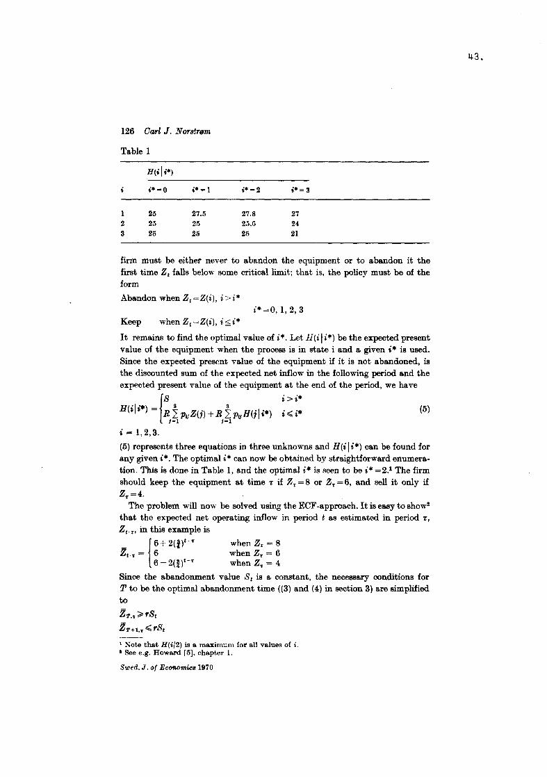
126 Carl J. Nor8!røm

Table 1

H('I·*)i .*-0 .*= l .*-2 ,*=3

1 25 27.5 27.8 272 25 25 25,6 243 25 25 25 21

firm must be either never to abandon the equipment or to abandon it thefirst time Zt falls below some critical limit; that is, the policy must be of theform

Abandon whenZt=Z(i), i>i*i* =0,1,2,3

Keep whenZt=Z(i),i~i*

It remains to find the optimal value of i*. Let H(ili*) be the expected presentvalue of the equipment when the process is in state i and a given i* is used.Since the expected present value of the equipment if it is not abandoned, isthe discounted sum of the expected net inflow in the following period and theexpected present value of the equipment at the end of the period, we have

Is i>i*

H(ili*) = R±PIIZ(j)+R±PIJH(ili*) i~i*i-l i-l

(5)

i=1,2,3.

(5) represents three equations in three unknowns and H(i Ii*) can be found forany given i*. The optimal i* can now be obtained by straightforward enumera-tion. This is done in Table l, and the optimal i* is seen to be i* =2.1 The firmshould keep the equipment at time T if Z ..= 8 or Z ..= 6, and sell it only ifZ..=4.

Thc problem will now be solved using the ECF -approaeh. It is easy to show2

that the expected net operating inflow in period t as estimated in period T,

Zt ..., in this example is- 16+2(1)1- ..Zt .. = 6

6-2(1)1-"

when Z .. = 8when Z .. = 6when Z .. = 4

Since the abandonment value St is a constant, the neeessary conditions forT to be the optimal abandonment time ((3) and (4) in section 3) are simplifiedtoZT.T~rStZT+1.T~rSt

l Note that H(i/2) is a maximum for all values of i.I See e.g. Howard [5), chapter 1.

Swed. J. of Ecmwmics1970

43.

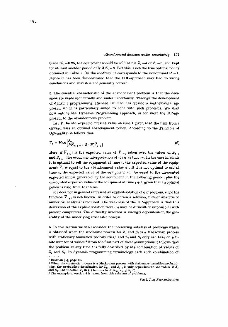
44.

Abandonment decision 'u/IIMr uncertainty 127

Since rSt=6.25, the equipment should be sold at T if Z.,.=4 or Z.,.=6, and keptfor at least another period only if Z.,. =8. But this is not the true optimal policyobtained in Table 1. On the contrary, it corresponds to the nonoptimal i* = 1.Hence it has been demonstrated that the ECF-approach may lead to wrongconclusions and that it is not generally correct.

5. The essential characteristic of the abandonment problem is that the deci-sions are made sequentially and under uncertainty. Through the developmentof dynamic programming, Richard Bellman has created a mathematical ap-proach which is particularly suited to cope with such problems. We shallnow outline the Dynamic Programming approach, or for short the DP-ap-preach, to the abandonment problem.

Let V t be the expected present value at time t given that the firm from tonward uses an optimal abandonment policy. According to the Principle ofOptimality- it follows that

V = Max {ST_ -T RZT+1-T + R· E[VT+1J

Here E[V HI] is the expected value of VHI taken over the values of ZH1

and SH1. The economic interpretation of (6) is as follows. In the case in whichit is optimal to sell the equipment at time T, the expected value of the equip-ment V.,. is equal to the abandonment value S.,.. If it is not optimal to sell attime T, the expected value of the equipment will be equal to the discountedexpected inflow generated by the equipment in the following period, plus thediscounted expected value of the equipment at time T+ l, given that an optimalpolicy is used from that time.

(6) does not in general represent an explicit solution of our problem, since thefunction VHI is not known. In order to obtain a solution, further analytic ornumerical analysis is required. The weakness of the DP-approach is that thisderivation of the explicit-solution from (6) may be difficult or impossible (withpresent computere). The difficulty involved is strongly dependent on the gen-erality of the underlying stochastic process.

(6)

6. In this section we shall consider the interesting subclass of problems whichis obtained when the stochastic process for Zt and St is a Markovian processwith stationary transition probabilities.s and Zt and St only can take on a fi-nite number of values," From the first part of these assumptions it follows thatthe problem at any time t is fully described by the combination of values ofZt and St. In dynamic programming terminology each such combination of

l Bellman [1], page 83.S When the stochastic process is a Markovian process with stationary transition probabil-ities, the probability distribution for ZtH and StH is only dependent 'on the values of Ztand St. The function Ft in (1) reduces to F(Zt+l' SI+lIZt. St).a The example in section 4 is ta.ken from this subcla.ss of problems.


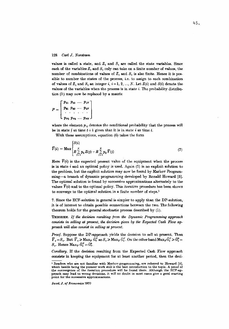
128 Carl J. Norstrøm

values is called a state, and Zt and St are called the state variables. Sinceeach of the variables Zt and Slonly can take on a finite number of values, thenumber of combinations of values of ZI and St is also finite. Hence it is pos-sible to number the states of the process, i.e. to assign to each combinationof values of Zt and St an integer i, i= 1,2, ... , N. Let Z(i) and Sei) denote thevalues of the variables when the process is in state i. The probability distribu-tion (l) may now be replaced by a matrix

P=

where the element PI} denotes the conditional probability that the process willbe in state i at time t + l given that it is in state i at time t.

With these assumptions, equation (6) takes the form

jS(i)Vei) = Max N N_

R 2: PlJZ(i) +R 2: Pli Vei)i-l }-l

(7)

Here Vei) is the expected present value of the equipment when the processis in state i and an optimal policy is used. Again (7) is no explicit solution tothe problem, but the explicit solution may now be found by Markov Program-ming-a branch of dynamic programming developed by Ronald Howard [5].The optimal solution is found by successive approximations alternately to thevalues Vei) and to the optimal policy. This iterative procedure has been shownto converge to the optimal solution in a finite number of steps.!

7. Since the ECF-solution in general is simpler to apply than the DP-solution,it is of interest to obtain possible connections between the two. The followingtheorem holds for the general stochastic process described by (l).

THEOREM. If the decision resuUing from the Dynamic Programming approachcon8ist8 in selling at present, the decision given by the Expected Cash Flow ap-proach will also consist in selling at present.

Proof. Suppose the DP-approach yields the decision to sell at present. ThenVT=ST' But VT~MaxT Gi soST~MaxTG;. On theotherhandMaxTG;~~=ST' Hence MaxT G; = m.Corollary. If the decision resulting from the Expected Cash Flow approachconsists in keeping the equipment for at least another period, then the deci-

1Readers who a:re not familiar with Markov-programming, are referred to Howard [6],which beside being tp.e pioneer work still is the best introduction to the topic. A proof ofthe convergence of the iteration procedure will be found there. Although the ECF-ap.proach may lead to wrong decisions, it will no doubt in most cases give a good startingpoint for the successive approximations.


45.

46.

Abandonment decision under uncertainty 129

sion given by the Dynamic Programming approach will also consist in keepingthe equipment for at least another period.'

Due to the corollary it is not necessary to find the correct optimal policywhen the optimal decision according to the ECF-approach is to keep theequipment.

8. As will be clear from the previous sections, we have not obtained a feasibleprocedure which generally solves the abandonment problem under uncertainty.sDynamic programming will lead to correct solutions, but may be unfeasibledue to the amount of numerical calculations required. If the stochastic processis a Markov process with stationary transition probabilities and finite statespace, thenMarkov programming may be used. Other approaches whichhave not been considered here, are applicable under other assumptions.t TheECF-approach is demonstrated to give incorrect results, but will no doubt usu-ally be a good approximation. As the theorem in section 7 shows, the ECF-approach leads to a tendency too sell too soon. When the optimal decision ac-cording to this approach is to keep the equipment, this decision is known to becorrect even when the optimal policy is not known.

References

1. Bellman, R.: Dynamic Programming.Princeton University Press, Prince-ton, 1957.

2. Breiman, L.: Stopping rule problems,in Beckenbaeh (ed.) Applied Gom-binatorial Mathematics. J. Wiley &Son, 1964.

3. Dyl, E. A. & Long, H. W.: Abandonmentvalue and capital budgeting: Com-ment. Journal of Finance XXIV,no. l, 1969.

4. Hart, A. G.: Anticipations, uncertaintyand dynamic planning. Studies inBusiness Administration XI (1940).University of Chicago Press, 1940.

Also available as a Reprint of Eco-nomic Classics, Augustus M. Kelley,1951.

5. Howard, R.: Dynamic Programming andMarkov Processes. The TechnologyPress of MIT and J. Wiley & Son,1960.

6. Robichek, A. A. & Van Horne, J. C.:Abandonment Value and CapitalBudgeting. Journal of Finance XXII,no. 4,1967.

7. Robichek, A. A. & Van Horne, J C.:Abandonment value and capital budg-eting: Reply. Journal of FinanceXXIV, no. l, 1969.

1The theorem and corollary do of course hold for the example in section 4 as the readermay readily verify.J Even when we disregard problems like risk aversion and estimation of probability dis-tributions.I In particular the reader is referred to the theory of Optimal Stopping Rules. For an ex-position of this theory, see Breiman [2].

Swed. J. of ECOflomics1970

WHEN TO DROP A PRODUCT: 47.

THE ABANDONMENT DECISION UNDER ATOMISTIC COMPETITION*

l. Introduction

The decision to drop unprofitable products forms an important

part of the overall marketing strategy. Excellent discussions

of the many aspects of this decision are given by Alexander [l]and Kotler [6]. This paper is more narrow. The abandonment

of a product is in principle a capital budgeting problem,

and this will be the approach taken. More specifically we

shall develop a capital budgeting model for the abandonment

decision of an atomistic firm when the future prices of the

product form a stochastic process. Allthough many firms

are not atomistic, this may be a fair approximation of

the situation at the end of a product 's life, when many close. . k lsubstltutes are ln the mar et.

The paper is organized as follows. The model is outlined

in section 2. In section 3 the optimal production policy

and the resulting net operating income is derived. The

abandonment decision is discussed in section 4. In section 5some consequences of the abandonment decision are discussed.

Finally, in section 6 some examples are given which illustrates

the material in the previous sections.

* Published lO Markedskommunikasjon, No.2. 1975.

48.

2. The Model

We consider a product, which is independent of the other

activities of the firm. To avoid sam mathematical difficul-

ties, time is regarded to be discrete and is partioned into

time periods of equal length. The following events take

place at the outset of each period in the given order.

(i) The firm decides whether to decrease the capacity to

produce the product.

(ii) The firm decides how much to produce in the period.

(iii) A chance event occurs which determines the price of

the product during the period.

A more detailed description of each event is given below.

(i) Capacity. Let.

kt - capacity at the outset of period t

Yt - decrease in capacity at the outset of period t.

The capacity prevailing during period t is consequently kt - Yt'

This also forms the beginning capacity of next period, i.e.2

(l) o <

From the sale of the capacity the firm receives an amount sYt '

where s is a constant. The cash inflow (or outflow if s

is negative) takes place at the beginning of the period.

49 .:

(ii) Production. Further assumptions on the cost function

will be given in the next section.

(iii) Price. Let

p - the price at the beginning of the period,t

the beginning price.

qt - the price prevailing during the period, the prevailing

price.

We shall let the continuous function F(qlp) be the

probability distribution of the prevailing price q for a

given beginning price p. Prices are assumed to be bounded

above. The prevailing price in period t forms the

beginning price in period t+l, Pt+l = qt' Hence the prices

form a stationary Markov process. There are

two natural cases for the domain of

(a) Continuous case. The domain is an interval [a,S]

(a may be _00 but S is finite), and

(2) F(qlp) = fqf(~lp)d~a

where f(qlp) is the probability density of q given p.

(b) Discrete case. The domain consists of a finite (or

infinite sequence of points {pel), p(2), ..., peN)} and

the matrix

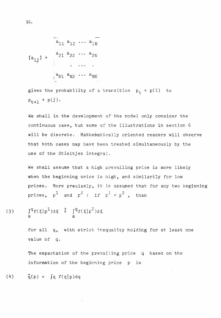
50.

all a12

[a..]a2l a22=lJ

l aNl aN2!

gives the probability of a transition Pt = p(i) to

Pt+l = p(j).

We shall in the development of the model only consider the

continuous case, but some of the illustrations in section 6will be discrete. Mathematically oriented readers will observe

that both cases may have been treated simultaneously by the

use of the Stieltjes integral.

We shall assume that a high prevailing price is more likely

when the beginning orice is high, and similarilY for low

prices. More precisely, it is assumed that for any two beginning

prices, lP and 2

P than

( 3 ) >

for all q, with strict inequality holding for at least one

value of q.

The expactation of the prevailing price q based on the

information of the beginning price p is

(4) q(p) = Jq f(qlp)dq

51.

The expectation is a continuous function of the beginning

price, and from assumption (3) it is seen also to be

strictly increasing.

The objective of the firm is to maximize the expected present

value of all future cash flows. The cost of capital is

assumed to be given and equal to r in each period. The

discount factor R is defined as l/(l+r).

3. The Production Decision

We note as a preliminary observation that the quantity

produced has no influence on future periods. It may be

classified as a static or short run decision.

In cost accounting a usual assumption is that total short run

costs consist of fixed costs and variable costs which increase

linearly with output. If in addition it is assumed that there

are constant returns to scale in the long run, the cost

function may be written in the form

( 5 ) C(x, k-y) = (c-b)x + bek-y) , O < x < k-y.

Here x is output, (k-y) is the capacity, and the constants

(c-b), b and c denote respectively average variable costs,

average fixed costs at full capacity and average total costs

at full capacity.

52.

The expected net operating income at the outset of a periodbefore the prevailing price is known, but after an eventualdecrease in capacity, is

(6) n(p, k-y) = q(p)x - (c-b)x - bek-y).

The production pOlicy takes the simple form of producingnothing if the expected price is less than average variablecosts and to produce up to capacity when the expected priceexeeds this cost. In terms of the beginning price it isoptimal to produce nothing when this price is less or equal

.to a certain level w, and to produce at full capacitywhen it exeeds this level.3 Defining

rr(p)when <p w

- c when p > w

the optimal expected net operating income may be written

(8) n*(p, k-y) = rr(p)(k-y).

rr(p) is the expected net operating income pr. unit ofcapacity and is a continuous and monotonically increasingfunction of the beginning price p.

4. The Abandonment Decision

The decision to decrease the capacity has an influence on thestate in future periods. The determination of the optimal

53.

pOlicy is a sequential decision problem. Such problems arewell suited for the use of dynamic programming, which willbe the mathematical approach taken.

If the net operating income takes place at the end of theperiod, it follows from the description of the model insection 2 and (8) that the expected present value of the cashflow in the first period is

(9) sy + Rrr(p)(k-y) ,

where the first term represents the cash flow from sale ofcapacity. We define the V(p,k) to be the expected presentvalue of all future cash flows from the product with anoptimal abandonment pOlicy. Proceeding formally from thePrinciple of Optimality4 it follows from (l) and (9) that

(10) V(p,k) = ~a~ {sy + Rrr(p)(k-y)O=y=k

+ R f V(q,k-y)f(qlp)dq}

The first two terms on the right hand side represent the cashflow (9) of the first period, and the last term all latercash flows. The optimization is achieved by balancingimmediate and future gains, the latter being a function of thebeginning price and the beginning capacity of next period.Some results may now be derived from (10).

Proposition l. There exists a unique bounded and continuousfunction V(p,k) satisfying (10).

54.

This proposition may be derived from a general result inDenardo [4]. For a proof of a similar result, see Norstr¢m[9 ] .

Proposition 2. The expected present value of all futurecash flows is a linear homogeneous function of the beginningcapacity,

(11) V(p,k) = A(p)k,

where A(p) is a continuous and monotonically increasingfunction.

This proposition may be ierived by the method of successiveapproximations. See e.g. Norstr¢m [9] for a similar result.An alternative proof is given in Norstr¢m [8]. The resultis reasonable intuitively, since both the expected net operatingincome and the cash flow from sale of capacity are linear.A(p) is the average expected present value pr. unit ofcapacity.

Proposition 3. There exists an optimal abandonment policyy(p,k) of the form

rk for p s v(12) y(p,k) = ~

·0 for p > v,<,

where v is a real number.

55.

Proof. Substitute (11) into the right hand side of (10) anddifferentiate with respect to y.

The form of the optimal abandonment policy is a consequenceof the assumptions of atomistic competition and the coststructure.5

In general the constant in (12) must be found by some iterativeprocedure, e.g. by successive approximations, or, in the discretecase, by Markov programming. However, an explicit solutionmay be found for the special case that the prices never increase.

First, we note that there are two possibilities with respectto the relation between the abandonment and the productiondecision. If v is less than w, it will be optimal to keepthe capacity forever without production when p falls below w.If v is greater than w, it is optimal to produce up to fullcapacity until the product is abandoned. It may be shownthat (under non-increasing prices) w > v if and only if thescrap value of capacity is negative with an absolute valuegreater than fixed cost divided by the interest rate, s < -b/r.

Proposition 4. Assurne that >s = -b/r and that prices arenon-increasing. Then it is optimal to abandon the productthe first time the expected prevailing price falls below thesum c+rs.

This proposition follows from a well known result in Stopping-rule problems.6 It is also easy to see intuitively. Thedifference between the expected present value of abandoningthe product after one period and abandoning it now is

56.

(13 ) R[q(p) - (c+rs)]

When (13) is positive, it pays to wait at least one period.

When (13) is negative, the expected value of waiting one

period is negative, and since prices are non-increasing the

same will be true for any future period.

In the general case when prices are not necessarily non-increa-

sing, Proposition 4 does not hold. Instead we have

Proposition 5. It is never optimal to abandon the product

as long as the expected prevailing price is above c+rs, but

it may be optimal to keep the capacity if the expectation is

lower than this sum.

A proof of this proposition may be found in [7]. The reason

for this somewhat paradoxicalresult is an asymmetry in the

effect of price increases and decreases created by the

opportunity to abandon the product. A favorable prevailing

price will have an effect not only on the net operating

income in the present period, but also on the value of the

production capacity at the end of the period. The corresponding

negative effect on the value of capacity of an unfavorable

prevailing price is eliminated or reduced by the abandonment

of the product.

5. Some Consequences of the Abandonment Decision

!~~_~~~~_2[_~2~Q92Q~~Q!

In this section some of the implications of the abandonment

57.

decision. We shall first consider the time of abandonment,

which will be denoted T and obviously is a stochastic

variable. Not only the expected time of abandonment, but

the entire probability distribution of T, ought to be a

valuable input in the firm's planning. We define for p > v

the sequence of functions {gn(qlp)} by

(l4a) gl(qlp) = f(qlp)

(14b) gn(qlp) = JSf(ql~)gn_l(~lp)d~v

The function gn(qlp) denotes for a given beginning price p

the joint event that the prevailing prices are above v in

first (n-l) periods and that the prevailing price in the n'th

period has the value q. The probability that the product

will be abandoned at time n (the end of nlth or beginning

(n+l)'st period) is consequently

(15) Gn(vlp) = JVgn(qIP)dqa.

It is not always the case that

00

(16) l:n=l

G (vip)n = l

since there may be a positive probability of never abandoning

the product. If (16) holds, the expected time to avandonment is

58.

00

(17) T(p) = E nGn(v!p)n=l

However, as pointed out above, the entire

distribution of the time of abandonment ought to be of

interest to the firm.

In the previous section it was found that the expected present

value of all future cash flows from the product was A(p)k,

where k is the present-capacity. A(p) is consequently the

average and marginal expected present value pr. unit of capacity.

Clearly A(p) = s for <p = v.

If we for convenience assume that <w v (that it is never

it may be shown7 thatoptimal to keep the capacity idle)

for p > v

00

(18) A(p) = En=l

Rn {f(q-c)g (q!p)dq + sG (q!p)}n n

Keeping in mind (14) and (15) it is seen that the ntth term

in (18) represents the sum of the expected net operating

income pr. unit in the n'th period and the expected cash from

selling the unit at time n.

The function A(p) is of particular interest for the decision

to increase the capacity, a decision which is not discussed in

59.

8this paper. However, we shall derive an interesting andperhaps somewhat surprising result from (18). Differentiationwith respect to c gives9

(19) oA(p) 00

= L Rn Gn(Slp).o c n=l

Gn(Slp) denotes the probability that the beginning pricesof the n first periods will exeed v. Due to assumption(3) this probability is an increasing function of thebeginning price at the outset of the first period. It followsthat a cost increase or-decrease has less impact on the valueof the product when the price is low. In particular, a oneshot cost - reducing investment is more profitable when the priceis high than when it is low. This result contradicts statementslike "it is necessary to rationalize because prices are low",if these are made out from profit considerations. The economicargument behind the result is that the life of the costreducing investment is longer when the beginning price is high.

It has often been an implicit assumtion in much of the economicliterature that uncertainty is undesirable. It will bedemonstrated that this is not necessarily true in the presentcase. We assume first that the prices qt' qt+l'stationary process with independent increments. To be consistent

is a

with the assumptions for existence and uniqueness in Propositionl, it is further assumed that prices are nonincreasing. Let the

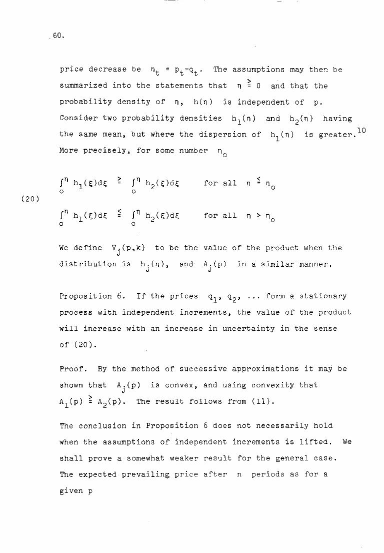
60.

price decrease be nt = Pt-qt' The assumptions may then besummarized into the statements that >n = O and that theprobability density of n, hen) is independent of p.

Consider two probability densities hl(n)the same mean, but where the dispersion of

and h2(n) having10hl(n) is greater.

More precisely, for some number no

> for all <n(20)

< for all n > no

We define V.(p,k) to be the value of the product when theJ

distribution is h.(n), and A.(p) in a similar manner.J J

Proposition 6. If the prices ql' q2' ... form a stationaryprocess with independent increments, the value of the productwill increase with an increase in uncertainty in the senseof (20).

Proof. By the method of successive approximations it may beshown that Aj(P) is convex, and using convexity that

>Al(p) = A2(p). The result follows from (11).

The conclusion in Proposition 6 does not necessarily holdwhen the assumptions of independent increments is lifted. Weshall prove a somewhat weaker result for the general case.The expected prevailing price after n periods as for agiven p

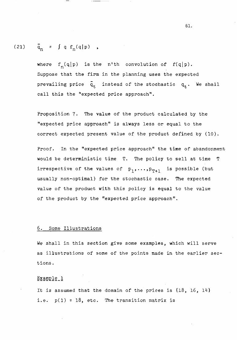
61.

(21) = ,

where fn(q[P) is the ntth convolution of f(q[p).Suppose that the firm in the planning uses the expectedprevailing price qt instead of the stochastic qt' We shallcall this the "expected price approach".

Proposition 7. The value of the product calculated by the"expected price approach" is always less or equal to thecorrect expected present value of the product defined by (10).

Proof. In the "expected price approach" the time of abandonmentwould be deterministic time T. The pOlicy to sell at time Tirrespective of the values of Pl, ...,PT+l is possible (butusually non-optimal) for the stochastic case. The expectedvalue of the product with this policy is equal to the valueof the product by the "expected price approach".

6. Some Illustrations

We shall in this section give some examples, which will serveas illustrations of some of the points made in the earlier sec-tions.

It is assumed that the domain of the prices is {18, 16, 14}i.e. pel) = 18, etc. The transition matrix is

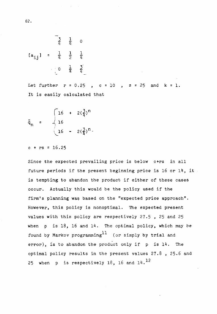
62.

3 l OIi Ii

[a..] l l l= Ii 2" IilJ

O l 3,- Ii Ii

Let further r = 0.25 c = 10 , s = 25 and k = L,It is easily calculated that

r16 + 2(t)n- !

qn = J._ 16I(16 2(t)n_

c + rs = 16.25

Since the expected prevailing price is below c+rs in allfuture periods if the present beginning price is 16 or 14, itis tempting to abandon the product if either of these casesoccur. Actually this would be the policy used if thefirm's planning wa~ based on the "expected price approach".However, this pOlicy is nonoptimal. The expected presentvalues with this pOlicy are respectively 27.5 , 25 and 25when p is 18, 16 and 14. The optimal policy, which may befound by Markov programmingll (or simply by trial anderror), is to abandon the product only if p is 14. Theoptimal pOlicy results in the present values 27.8 , 25.6 and25 when p is respectively 18, 16 and 14.12

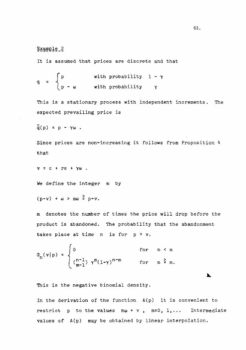
63.

It is assumed that prices are discrete and that

q =y- w

with probability

with probability

l - Y

This is a stationary process with independent increments. The

expected prevailing price is

q(p) = p - yw .

Since prices are non-increasing it follows from Proposition 4that

v = c + rs + yw

We define the integer m by

>(p-v) + w > mw p-v.

m denotes the number of times the price will drop before the

product is abandoned. The probability that the abandonment

takes place at time n is for p > v.

for n < m

for >n = m.

This is the negative binomial density.

In the derivation of the function A(p) it is convenient to

restrict p to the values mw + v) m=O, l, ... Intermediate

values of A(p) may be obtained by linear interpolation.

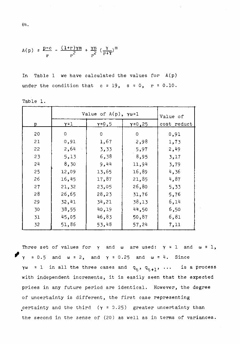
64.

A(p) = E=£ _ (l+r)ym + ~ (_I_)m2 2 r+Yr r r

In Table l we have calculated the values for A(p)under the condition that c = 19, s = O, r = 0.10.

Table l.

Value of A(p), yw=l Value ofp y=l y=0,5 y=0,25 cost reduct20 O O O 0,9121 0,91 1,67 2,98 1,7322 2,64 3,33 5,97 2,4923 5,13 6,38 8,95 3,1724 8,30 9,44 11,94 3,7925 12,09 13,65 16,89 4,3626 16,45 17,87 21,85 4,8727 21,32 23,05 26,80 5,3328 26,65 28,23 31,76 5,7629 32,41 34,21 38,13 6,1430 38,55 40,19 44,50 6,5031 45,05 46,83 50,87 6,8132 51,86 53,48 57,24 7,11

Three set of values for y and w are used: y = l and w = l,,Y = 0.5 and w = 2, and y = 0.25 and w = 4 . Sinceyw = l in all the three cases and qt' qt+l' is a processwith independent increments, it is easily seen that the expectedprices in any future period are identical. However, the degreeof uncertainty is different, the first case representingcertainty and the third (y = 0.25) greater uncertainty than•the second in the sense of (20) as well as in terms of variances.

65.

(The variances are respectively O, l, and 3). According toProposition 6 the values of A(p) will be smallest for y = land largest for y = 0.25 for all values of p. This resultis confirmed in the table.

It may be shown that a cost reduction will have the sameeffect as a price increase in the case of a process withindependent increments. A reduction ~ in average total costswill hence increase the expected present value of the productby

[A(p+~) - A(p)]k.

In the last column of Table l we have calculated the valuesof [A(p+~) - A(p)] for ~ = l, Y = l, w = l and valuesof c, sand r as specified above. The expected present valueof the cost reduction is seen to be an increasing function of p.

As in Example 2 it is assumed that the prices form astationary process with independent, but the domain is nowcontinuous with the density function

= -AnAe

It follows that

l= p - I

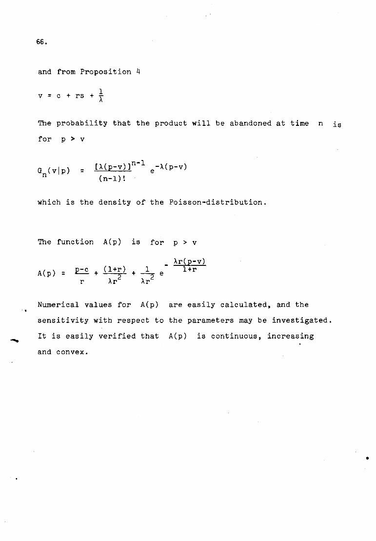
66.

and from Proposition 4

lv = c + rs + I

The probability that the product will be abandoned at time n isfor p > v

=[A(p_v)]n-l(n-l)!

-A(p-V)e

which is the density of the Poisson-distribution.

The function A(p) is for p > v

Ar(E-v)A(p) £.:.£ + (l+r) l l+r= Ar2

+ -- er Ar2

Numerical values for A(p) are easily calculated, and the..sensitivity with respect to the parameters may be investigated.It is easily verified that A(p) is continuous, increasingand convex.

•

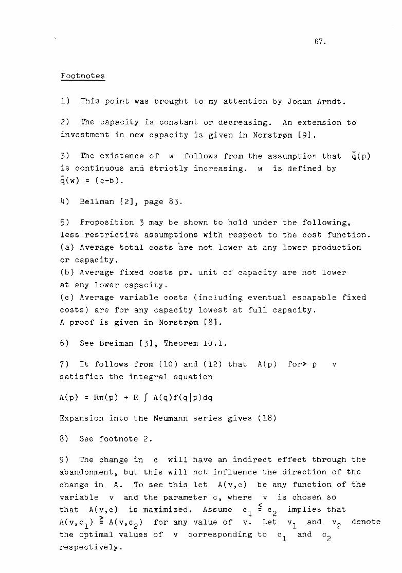
67.

Footnotes

l) This point was brought to my attention by Johan Arndt.

2) The capacity is constant or decreasing. An extension toinvestment in new capacity is given in Norstr¢m [91.

3) The existence of w follows from the as~umption that q(p)is continuous and strictly increasing. w is defined byq(w) = (c-b).

4) Bellman [2], page 83.

5) Proposition 3 may be shown to hold under the fOllowing,less restrictive assumptions with respect to the cost function.(a) Average total costs are not lower at any lower productionor capacity.(b) Average fixed costs pr. unit of capacity are not lowerat any lower capacity.(c) Average variable costs (including eventual escapable fixedcosts) are for any capacity lowest at full capacity.A proof is given in Norstr¢m [81.

6) See Breiman [31, Theorem 10.1.

7) It follows from (la) and (12) that A(p) for> p vsatisfies the integral equation

A(p) = Rn(p) + R f A(q)f(qlp)dq

Expansion into the Neumann series gives (18)

8) See footnote 2.

9) The change in c will have an indirect effect through theabandonment, but this will not influence the direction of thechange in A. To see this let A(v,c) be any function of thevariable v and the parameter c, where v is chosen so

A(v,c) is maximized. Assume < implies thatthat cl c2>A(v,cl) = A(v,c2) for any value of v. Let vl and v2 denotethe optimal values of v corresponding to cl and c2respectively.

68.

Then

Hence the secondary effect working through the decisionvariable may be ignored. See also Bellman [2], pp. 157-8.

la) See Rothschild and Stiglitz [la].

11) The best introduction to Markov programming is still theoriginal work, Howard [5].

12) A more detailed discussion of this example is given inNorstr¢m [7].

69.

~eferences

l. Alexander, R.S., The Death and Burial of 'Sick' Products,Journal of Marketing, April 1964.

2. Bellman, R., Dynamic Programming, Princeton UniversityPress, N.J. 1957.

3. Breiman, L., Stopping Rule Problems, in Applied CombinatorialMathematics, E.F. Beckenback (ed), John Wiley andSon, Inc., N.Y. 1964.

4. Denardo, E.V., Contraction Mappings in the Theory underlyingDynamic Programming, SIAM Review 9 (1967), 165-177.

5. Howard, R., Dynamic Programming and Markov Processes,The MIT Press and John Wiley & Son, Inc., N.Y. 1960.

6. Kotler, P., Phasing Out Weak Products, Harvard BusinessReview, March-April 1965.

7. Norstr¢m, C.J., The Abandonment Decision under Uncertainty,Swedish Journal of Economics 72 (1970), 124-129.

8. Norstr¢m, C.J., The Abandonment Decision under AtomisticCompetition, Manuscript, 1974.

9. Norstr¢m, C.J., Optimal Capital Adjustment under Uncertainty,Journal of Economic Theory 8 (1974), 139-148.

10. RothsctUld, M. and J.E. Stiglitz, Increasing Risk:I A definition, Journal of Economic Theory 2 (1970),66-84.

70.A STOCHASTIC MODEL FOR THE GROWTHPERIOD DECISION IN FORESTRY*

l. Introduction

The growth period decision is a familiar problem in economictheory, known from the work of Jevons, Wicksell and IrvingFisher. The aim of this paper is to strengthen the realism ofthe model when applied to forestry, by explicit recognition ofuncertainty in the future values of the trees.l In order toinvestigate whether this extension may be important, acomparison is made between a policy which takes account ofuncertainty and one where uncertainty is ignored.

2. The Model

In the deterministic growth period model the objective is tomaximize the present value

(l) WeT) = - C + (l+r)-T[g(T) + Gl

where

get) - the net value of the forest stand when cut t years old.C - the cultivation cost, e.g. cost of seedling.G - the value of land.2

r - the market interest rate.T - the time the forest stand is cut.

The model is well known, and will not be elaborated here.3

Forthcoming in the Swedish Journal of Economics.

71.

The first task in the construction of a stochastic model is toidentify the main sources of uncertainty. The most criticalfactor in the determination of the optimal time to cut a foreststand is the value increase from waiting one period,

(2) g(t+l) - get).

This value is normally decomposed into three components: theincrease in total volume, the quality increase due to the largerdimension of each tree, and the increase or decrease in thebasic price of timber. Due to research done by forest econo-mists, reasonably good estimates exist for the volume andquality increase, dependent on such factors as age, fertilityof the soil, intensity of thinning. There are, however,very substantial fluctuations in the price of timber from seasonto season.4 These fluctuations are here taken to be the onlysource of uncertainty.

The basic assumption of the model is that the value of theforest stand at a future time t is a product

where fet) is a deterministic growth function and Pt astationary stochastic process. The two elements in the productmay be given various economic interpretations. We shall letfet) represent the expected value of the asset and Pt anindex reflecting the variation in the basic price of timberrelative to the long run expectation.

In addition to the above basic assumption, we shall in this andthe next three paragrap~es make some others, which are notessential for the approach. - It is assumed that the

72.

sequence PI' P2"'" is a stationary Markow process with afinite state space P = {p(I),p(2), ...,p(N)}, wherepel) > p(2» ...> peN). The transition probabilities will bewritten in the form of a transition matrix

all al2 o • o alN

(4) A a21 a22 • • o a2N=• • o

aNI aN2 • • o aNN

where the element a .. denotes the probability that~J

Pt+l = p(j) given that Pt = p(i).

The cutting policy will depend on the information available tothe decisionmaker. Several alternative assumptions are possible,and the'choice must depend on the real situation at hand. Itis assumed here that is fully known, when the decision

t is taken.Swhether to sell at time

The objective is taken·to be maximization of the expectedpresent value of future cash flows. This is the obvious genera-lization of the objective in the deterministic model, butcontains the weakness that the possibility of risk aversion isignored.

Two cases will be consideres with respect to the value of land.In the first the value of land is taken to be a given functionof the state of the price index Pt;

(S) Gt = G(i) when Pt = p(i).

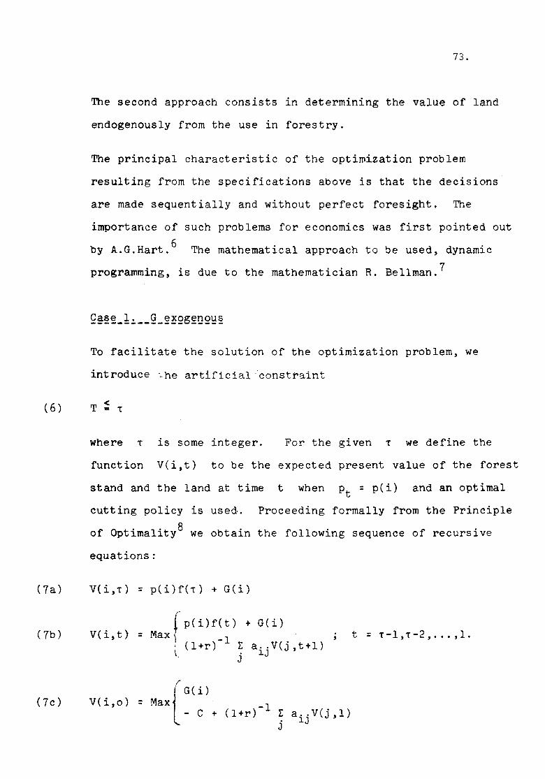
73.

The second approach consists in determining the value of landendogenously from the use in forestry.

The principal characteristic of the optimization problemresulting from the specifications above is that the decisionsare made sequentially and without perfect foresight. Theimportance of such problems for economics was first pointed out

6by A.G.Hart. The mathematical approach to be used, dynamicprogramming, is due to the mathematician R. Bellman.7

To facilitate the solution of the optimization problem, weintroduce ;·he artificial'constraint

(6 ) <T = -r

where -r is some integer. For the given -r we define thefunction V(i,t) to be the expected present value of the foreststand and the land at time t when Pt = p(i) and an optimalcutting policy is used. Proceeding formally from the Principleof Optimality8 we obtain the following sequence of recursiveequations:

(7a) V(i,-r) = p(i)f(-r) + G(i)

(7b) V(i,t)(p(i)f(t) + G(i)

= Max t -li (l+r) ta ..V (j , t+l)~ . lJ. J

t = -r-l,-r-2,... ,1.

(7c) V(i,o)f

t G( i)= Max

- C + (l+r)-l t a ..V(j,l)j lJ

74.

The values of V(i,t) are given by (7) for all i and t.To formulate an optimal policy define the sets

(8) St = {p(i) EP1V(i,t) = p(i)f(t) + G(i)}

t = 1,2, ... , T, and similarily for S .o In presence of theartificial constraint (6), the following pOlicy is optimal:

Cut the forest stand the first period the price index Ptbelongs to the set St'

In general the values of V(i,t) and the sets St will dependon the number T in (6). Ideally T should be chosen largeenough to make it uneconomical to keep the forest stand beyondthis date regardless of the value of p. This is not always

T

possible, but it may be shown under fairly broad conditionsthat V(i,t) for any fixed t can be made arbitrar11yclose tothe true values by choosing T sufficiently large.

We shall now consider the case that the value of land is notgiven, but must be derived. For simplicily forestry is assumedto be the only economic alternative.

The solution is obtained by solving a sequence of optimizationproblems with the value of land taken from the previous problemin the sequence. For a given value of T

(9a) G(i,O) = O

(9b) V(i,T,n) = p(i)f(T) + G(i,n)

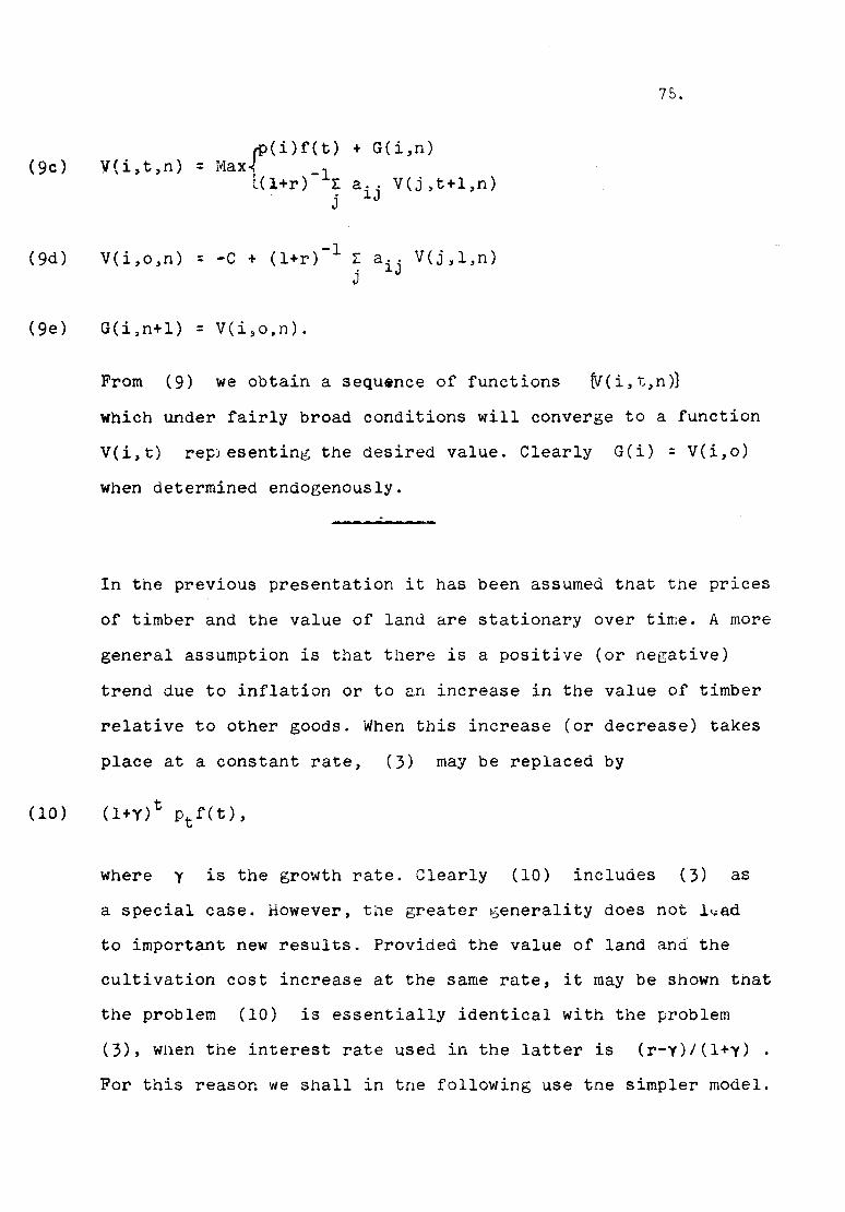
75.

(9c)f(i)f(t) + G(i,n)

V(i,t,n) = ~laxl<l+r)-lr a .. V(j)t+l,n)j l.J

V(i,o,n) : -C + (l+r)-l r a .. V(j )l,n)j l.J(9d)

(ge) G(i.n+l): V(i,o,n).

From (9) we obtain a sequ~nce of functions tv ( i ,t ,n »)

which under fairly broad conditions will converge to a functionV(i,t) re~}esenting the desired value. Clearly G(i) : V(i,o)when determined endogenously.

In tne previous presentation it has been assumed that the pricesof timber and the value of land are stationary over time. A moregeneral assumption is that there is a positive (or negative)trend due to inflation or to an increase in the value of timberrelative to other goods. When this increase (or decrease) takesplace at a constant rate, (3) may be replaced by

where y is the growth rate. Clearly (10) includes (3) asa special case. However, the greater generality does not l~adto important new results. Provided the value of land and.thecultivation cost increase at the same rate, it may be shown thatthe problem (10) is essentially identical with the problem(3), wnen the interest rate used in the latter is (r-y)/(l+y).For this reason we shall in tne following use the simpler model.

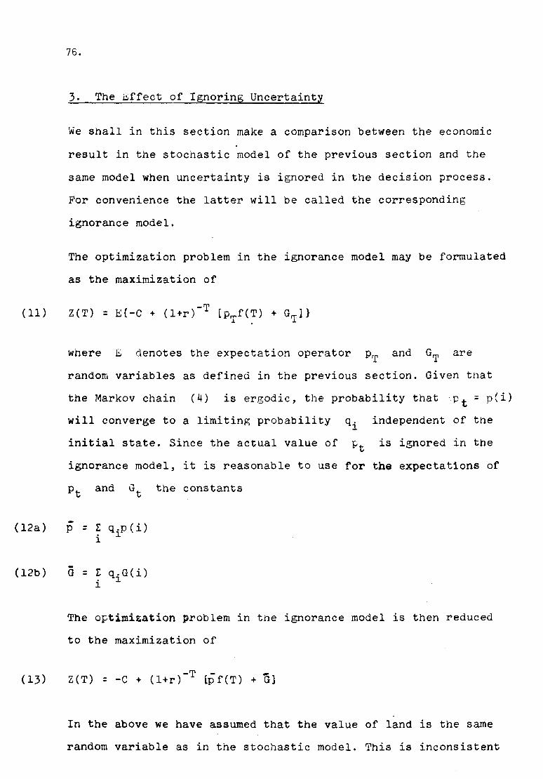
76.

3. The Effect of Ignoring Uncertainty

We shall in this section make a comparison between the economicresult in the stochastic model of the previous section and thesame model when uncertainty is ignored in the decision process.For convenience the latter will be called the correspondingignorance model.

The optimization problem in the ignorance model may be formulatedas the maximization of

where E denotes the expectation operator and arerandom variables as defined in the previous section. Given thatthe Markov chain (4) is ergodic, the probability that 'Pt = p(i)will converge to a limiting probabilityinitial state. Since the actual value of

q.~

independent of theis ignored in the

ignorance model, it is reasonable to use for the expectations ofand G t the constants

(12a)

(12b)

The optimitation problem in the ignorance model is then reducedto the maximization of

( 13) Z(T ) = - C + (l +r )-T lp f (T ) + G]

In the above we have assumed that the value of land is the samerandom variable as in the stochastic model. This is inconsistent

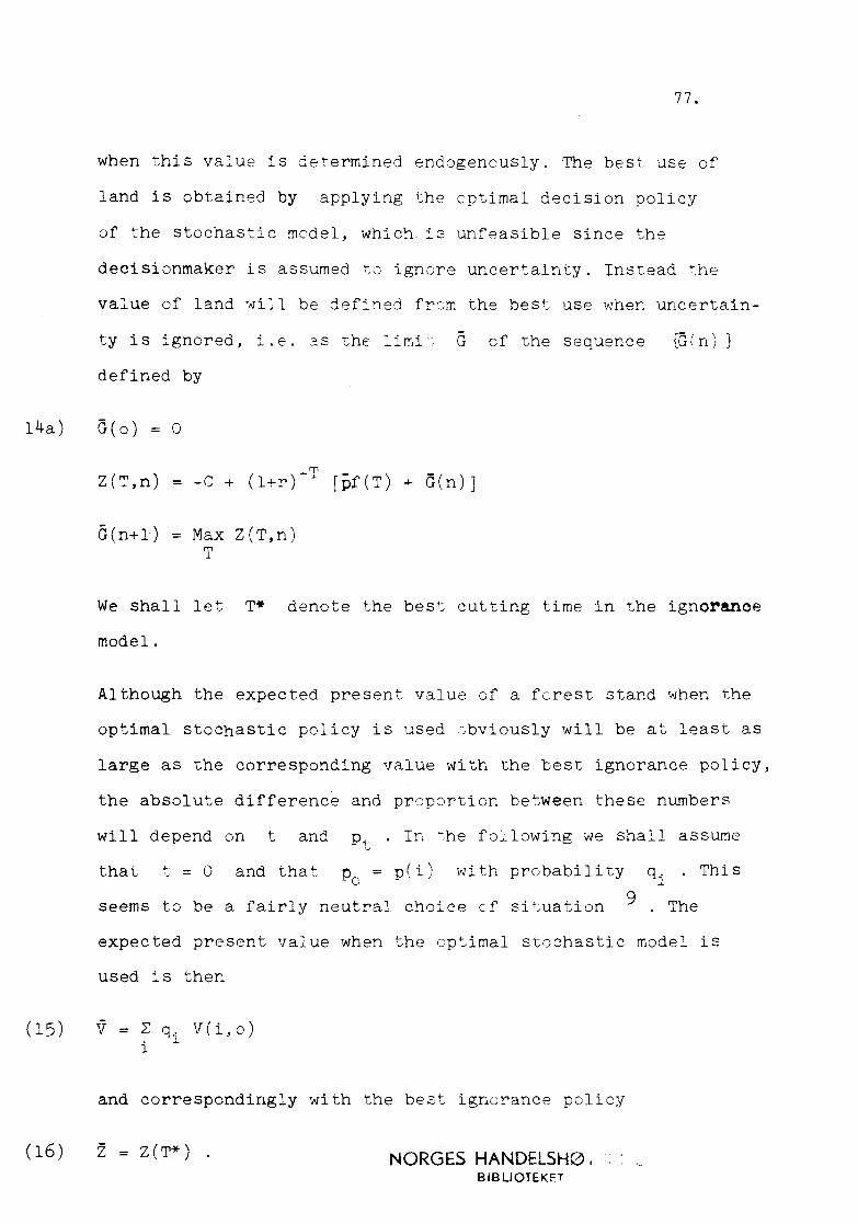
77.

when this value is determined endogenously. The best use of

land is obtained by applying the optimal decision policy

of the stochastic model, which. is unfeasible since the

decisionmaker is assumed to ignore uncertaint.y. Instead the

value of land l~ill be defined fr~m the best use when uncertain-

ty is ignored, i.e. as the limit G of the sequence (G(n) }

defined by

14a) G(o) = O

Z(T,n)_IT'

[pf(T) G(n)]= -C + (l+r) .l- +

G(n+l) = Max Z(T,n)T

We shall let T* denote the best cutting time in the ignoranoemodel.

Al though the expected present value of a fcrest stand when the

optimal stochastic policy is used ~bviously will be at least as

large as the corresponding value with the best ignorance policy,

the absolute difference and proportion between these numbers

will depend on t and Pt . In ~he following we shall assume

that t = O and that Pc = pri) with probability qi . This

seems to be a fairly neutral choice cf situation 9 . The

expected present value when the optimal stochastic model is

used is then

(15) V = ~ qi V(i,o)i

and correspondingly with the best ignorance policy

(16) Z = Z(T*) . NORGES HANDELSHØ,BIBLIOTEKFT

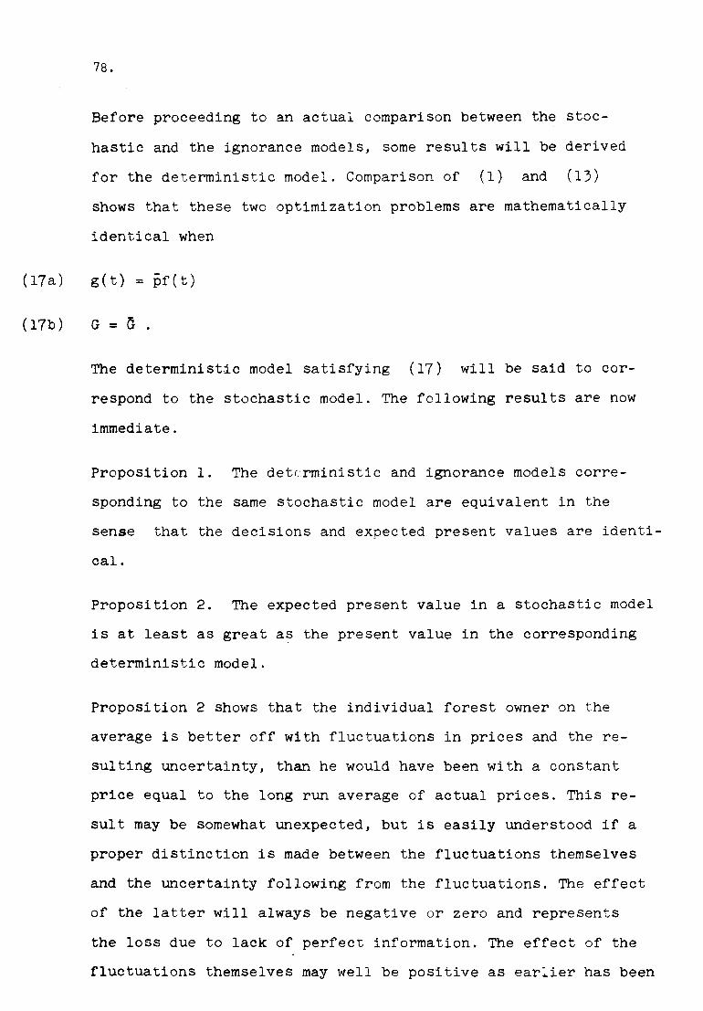
78.

Before proceeding to an actual comparison between the stoc-hastic and the ignorance models, some results will be derivedfor the deterministic model. Comparison of (l) and (13)shows that these two optimization problems are mathematicallyidentical when

(17a)

(17b)

g (t) = pf (t)

G = n .

The deterministic model satisfying (17) will be said to cor-respond to the stochastic model. The following results are nowimmediate.

Proposition l. The deterministic and ignorance models corre-sponding to the same stochastic model are equivalent in thesense that the decisions and expected present values are identi-cal.

Proposition 2. The expected present value in a stochastic modelis at least as great as the present value in the correspondingdeterministic model.

Proposition 2 shows that the individual forest owner on theaverage is better off with fluctuations in prices and the re-sulting uncertainty, than he would have been with a constantprice equal to the long run average of actual prices. This re-sult may be somewhat unexpected, but is easily understood if aproper distinction is made between the fluctuations themselvesand the uncertainty following from the fluctuations. The effectof the latter will always be negative or zero and representsthe loss due to lack of perfect information. The effect of thefluctuations themselves may well be positive as ear:ier has been

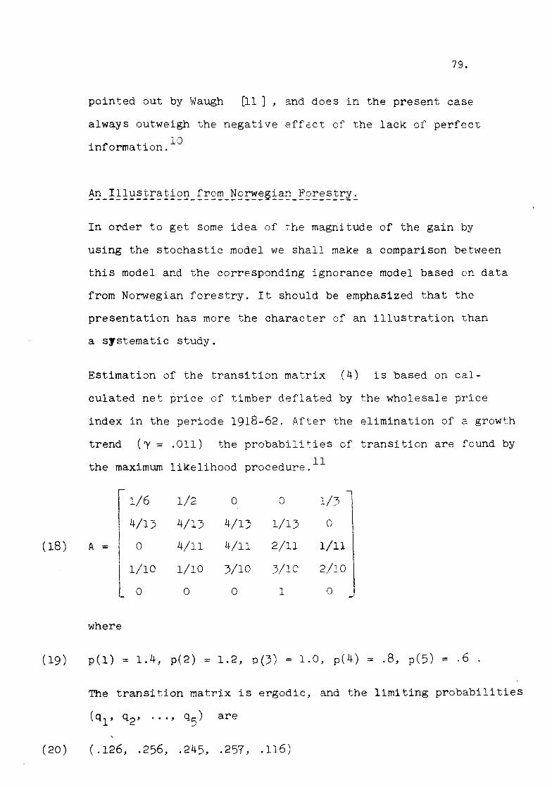
79.

pointed out by Waugh [11], and does in the present case

always outweigh the negative effect of the lack of perfectinformation. 10

In order to get some idea of the magnitude of the gain by

using the stochastic model we shall make a comparison between

this model and the corresponding ignorance model based en data

from Norwegian forestry. It should be emphasized that the

presentation has more the character of an illustration than

a systematic study.

Estimation of the transition matrix (4) is based on cal-

culated net price of timber deflated by the wholesale price

index in the periode 1918-62. After the elimination of a growth

trend (ry = .011) the probabilities of transition are found by11the maximum likelihood procedure.

.,r 1/61/2 O O 1/3

4/13 4/13 4/13 1/13 O

(18) A = l O 4/11 4/11 2/11 l/IlII

1/10 l/1O 3/10 3/10 2/10I ' ~

L O O O " O I.1. ~

where

(19) p(l) = 1.4, p(2) = 1.2, p(3) = 1.0, p(4) = .8, p(5) = .6 .

The transition matrix is ergodic, and the limiting probabilities

(20) (.126, .256, .245, .257, .116)

80.

and

(21) P = 1.004 .

The growth function fet) will depend on such factors asthe quality of the soil, intensity of thinnings etc .. However,since growth functions have the same general shape, the choicewill be of small importance in the comparison. We shall use anexample taken from Risvand [7] . See Table l.

Table l

2. Thinning 3. Value ofl. Age value remaining

stand

34 O 38.4638 O 146.6842 O 301.8746 -1.03 444.0650 O 647.2954 133.81 686.2558 O 909.6362 O 1,146.4166 O 1,397.8570 O 1,637.9774 O 1,881.58

Source: R1svand [7].There are two thinnings, one in the 46th an~ one in the 54th

.~

year.We shall restrict the final cut to the years after thelast thinning. The growth in the value of the remaining stand,~

is in this period nearly linear, and the value& of the inter-mediate years are estimated by linear interpolation. The valueof l' used in the artificial constraint (6) is taken to be74 years.

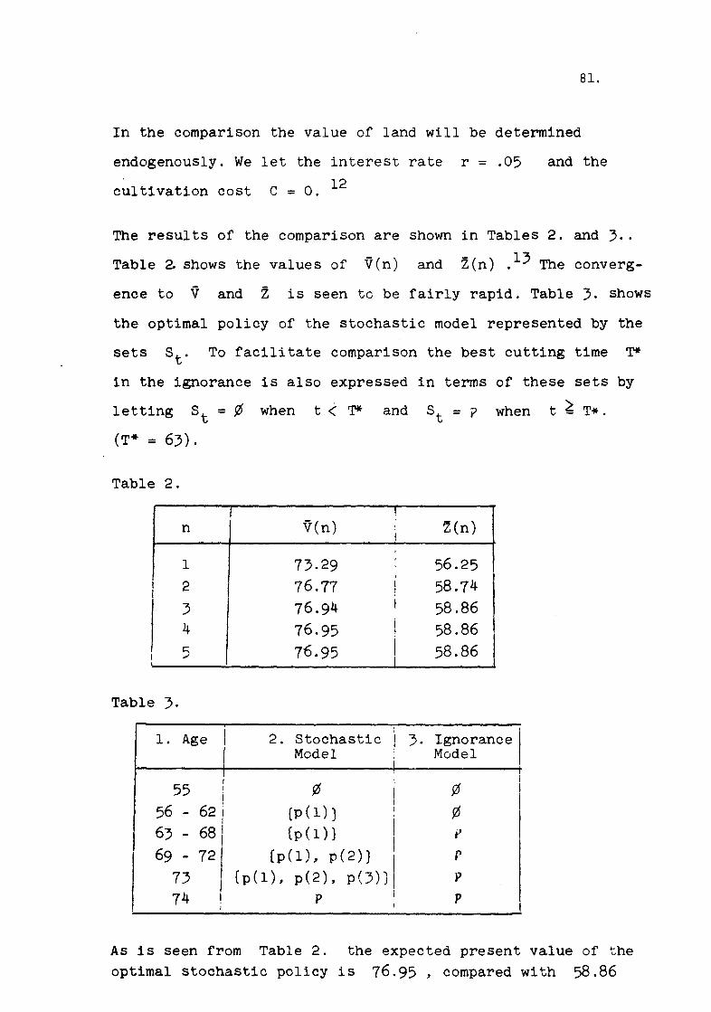
81.

In the comparison the value of land will be determinedendogenously. We let the interest rate r = .05 and thecultivation cost 12C = O.

The results of the comparison are shown in Tables 2. and 3..Table 2. shows the values of Ven) and Zen) .13 The converg-ence to V and Z is seen te be fairly rapid. Table 3. showsthe optimal policy of the stochastic model represented by thesets St' To facilitate comparison the best cutting time T*in the ignorance is also expressed in terms of these sets byletting St = ø when t <: T* and St = j> when t ~ T*.(T*=63).

Table 2.I !n Ven) , Zen)l,

,l

l 73.29 l 56.25l

I II 2 76.77 I 58.74I I

3 76.94 I 58.86

I 4 76.95 i 58.86I

II

5 76.95 I 58.86I I,

Table 3.I

1. Age I I2. Stochastic I 3.,Model iIgnoranceModel

Ii

56 - 62 iI

63 - 68169 - 721

73 I74 !

i'

55 :I

(p ( l) ) 11

(p (l))

(p(l), p(2)) !(p(l), p(2), p(3))\

I

ø øø

p

rpp

As is seen from Table 2. the expected present value of theoptimal stochastic policy is 76.95, compared with 58.86

82.

when uncertainty is ignored. The increase in present value is17.04 , or 30.3 per cent.

4. Conclusion.

In the illustration above we have neglected several factorsof real life, and the result must hence be interpreted withsome care. None the less the comparison is a clear indicationof the importance of taking price fluctuations into accountin the determination of the final cut.

The stochastic model presented here may be further refined inseveral directions, e.g. by adding som constraints on thedecisionmaker's actions. Another posSibility is to add otherstate variables in order to improve the decisionmaker's in-formation about future prices, and in this way obtain a stillbetter policy. Either addition will, however, lead to greatincreases in computational requirements.

Footnotes:

*) The author would like to express his indebtness to severalmenmbers of the Norwegian Forest Research Institute, inparticular John Eid, Jens Risvand, Asbjørn SvendsrudRolf Sæther, and to Agnar Sandmo. Thanks also go to

andHelge

Gundersen, who carried out the computer programming.

83.

Footnotes continued

l) Although formally valid, the model is probably not arealistic stochastic representation for other growth processes,like wine-aging.

2) A more general approach would be to let the value of landbe a function of time.

3) Interested readers are referred to Lutz [4], Lutz andLutz [5] and Bierman [2].

4) See the study by Sæther [10], pp. 391-414.

5) This seems to be in reascnable agreement with the condi-tions in Norwegian forestry.-See Sæther [10], pp. 415-417for details.

6) Hart [3], especially chapter 4.

7) Bellman [l].

8) Bellman [l], p. 83.

9) The assumption may be greatly weakened with negligible conse-quences for the actual comparison below.

10)Oi

For discussion of Waugh s[6] and Waugh [12].

result, see Samuelson [8,9],

Il) The data are taken from the study by Sæther [10]. Thematrix is based on observation of 6 transitions from state l,13 from state 2, Il from state 3, 10 from state 4 and 4 fromstate 5.

12) The growth function in Table l. is derived under the condi-tion that r = .03 in which case T* = 74. The choice ofr = .05 is made in order to have T* somewhat smaller than T.

13) The definitions of ~(n) and Zen) are obvious extensionsof (15) and (16).

84.

References:

l. Bellman, R.: Dynamic Programming, Princeton UniversityPress, N.J. 1957.

2. Bierman, H. Jr.: The Growth Period Decision, ManagementScience, Vol. 14, No.6, February 1968.

3. Hart, A.G.: An t.t cLpa t t ons, Uncertainty and Dynamic Plan-ning, Studies in Business Administration XI (1940),University cf Chicago Press, 1940. Also available as aReprint of Economic Classics, Augustus M. Kelley, 1951.

4. Lutz, F.A.: The Criterion on Maximum Profits in theTheory of Investment, Quarterly Journal of Economics,Vol. LX, No. l, November 1945.

5. Lutz, F.A. and V.Lutz: The Theory of Investment of theFirm, Princeton University Press, Princeton, N.J., 1951.

6. Oi, W.Y.: The Consumer Does Benefit from Feasible PriceStability: A Comment, Quarterly Journal of Economics,Vol. LXXXVI, No.3, 1972.

7. Risvand, J.: Economic Analysis of Cutting ProgramsApplying Dynamic Programming, in Readings in ForestEconomics, (A.Svendrud, Ed.), 73-80, Universitetsforlaget,Oslo, 1969.

8. Samuelson, P.A.: The Consumer Does Benefit from FeasiblePrice Stability, Quarterly Journal of Economics, Vol.LXXXVI, No.3. August 1972.

9. Samuelson, P.A.: Rejoinder, Quarterly Journal of Economics,Vol. LXXXVI, No.3, August 1972.

85.

10. Sæther, R.: Supply of Industrial Softwood in Norway. AStatistical Inquiry into Annual Cuts and Factors AffectingQuantities Cut during the Period 1918-1960, NorwegianForest Research Institute, Vollebekk, Norway. Written inNorwegian with English Summary.

11. Waugh, F.V.: Does the Consumer Benefit from PriceInstability? Quarterly Journal of Economics, Vol. LVIII,602-14, August 1944.

12. Waugh, F.V.: A Comment.Quarterly Journal of Economics, Vol. LXXXVI, No.3,August 1972.

86.

Reprinted from JOl'R'IAL OF ECONOMIC THEORYAll Rights Reserved by Academic Press, New York and London

Vol. 8, No.2, June 1974Printed in Belgium

Optimal Capital Adjustment under Uncertainty*

CARL J. NORSTRØM

Norwegian School of Economics and Business Administration, 5(}()() Bergen, Norway

Received March 6, 1973

1. INTRODUCTION

The purpose of this article is to analyze the effect of existing capitalstock on the optimal investment policy of the firm under conditions ofuncertainty.Pionering work on the optimal capital adjustment of the firm under

certainty has been done by Arrow, Beckmann, and Karlin [3], and Eisnerand Strotz [6]. Their work has later been extended by other authors likeArrow [l, 2], Gould [7], Lucas [9,10], Rothschild [12], and Treadway [14].More recently Hartman [8] introduced uncertainty in a model withconstant returns to scale and strictly convex cost of adjustment.The article is organized as follows. After the presentation of the model

in Section 2, existence of an optimal investment policy is proved inSection 3. The connection between the static returns to scale and thevalue of the firm is established in Section 4. The implications for theoptimal investment policy are discussed in Section 5. It is assumed through-out that the firm's objective is to maximize the expected present value ofthe future cash flows, or in other words, that it is risk neutral.

2. THE MODEL

To avoid mathematical difficulties, time will be taken to be discrete.The situation of the firm at the beginning of period t is assumed to becompletely described by the capital stock K, and a finite-dimensionalvector P, . This vector may consist of elements like the price of the productproduced by the firm, the wage rate, parameters for the cost of investment,etc., in the current and a finite number of previous periods.

* This paper is an extension of a part of the author's licentiat thesis [lO]. The presentversion owes much to a stay at the University of Michigan, made possible by a scholar-ship from the Norway-American Association. The author is indebted to Karl Borch,Jan Mossin, Agnar Sandmo, Sidney G. Winter, Jr., and a referee for valuable comments.

139Copyright © 1974 by Academic Press, Inc.All rights of reproduction in any form reserved.

140 CARL J. NORSTRØM

The vector P, is restricted to lie in a bounded set 9. We let the functionF(PHI I Pt) defined on 9 X 9 be the conditional probability distributionof PHI given Pt. Hence the vectors P, , Pt+l , ••• form a stationary Markovprocess.The dynamic behavior of the capital stock is governed by

where o is the depreciation rate and It is the gross investment in period tmeasured in physical units. The cost of the gross investment is given by acost function C(It , PI). It is assumed that C(l, P) is continuous in P andtwice differentiable in I, that the first derivative Cl(/, P) ~ O and thatC(O,P) = O. Moreover the gross investment is assumed to be non-negative and bounded, i.e.,

where I is a given constant. The net operating profit of the firm in anyperiod is a given function g(Kt , Pt) of the capital stock and the vector P, .Any optimization necessary to obtain this function is assumed to be ofmyopic character. g(K, P) is taken to be continuous in P, twice differen-tiable in K, and bounded for finite K and P E 9.

The objective of the firm is to maximize the expected present value ofthe future net cash flow, that is, the expectation of

co

I Rt(g(Kt , Pt) - C(It , Pt)],t=l

where the initial capital stock Kl is given and R = (l + r)-1 is a discountfactor (O< R < 1).

3. EXISTENCE OF AN OPTIMAL INVESTMENT POLICY

It is known from the formulation of the model that the situation of thefirm at the beginning of period t is completely described by the capitalstock K, and the vector Pt. We define V(Kt, Pt) to be the expected presentvalue of all future cash flows of the firm, when an optimal investmentpolicy is used. In the absence of risk aversion the function will alsorepresent the value of the firm. Proceeding formally from the principle ofoptimality+ it is seen that

V(Kt, Pt) = sup R [g(Kt, Pt) - co., Pt)i,

+ f V(Kt+1, Pt+1) dF(Pt+1 I Pt)]. (4).CF'

1Bellman [4], p. 83.

87.

(1)

(2)

(3)

88.

OPTIMAL CAPITAL ADJUSTMENT 141

Here the two first terms on the right side represent the net cash inflow inthe present period, and the last term the expected present value of thetotal cash flow from next period onward. Using (1) and the fact thatPt+l enters only as a vector of integration, (4) may be reformulated as

VeK, P) = s~p R ) g(K, P) - C(l, P) + Ja> V[(1' - sv: + l, Y] dF(Y [ p)I,(S)

where for convenience subscripts have been dropped.It must be shown that the function VeK, P) exists and is unique.

In the proof we shall use the fact that the capital stock is bounded.

LEMMA 1. The stock of capital in any period lies in the interval [O,K],where K = max [Kl , o-IJ].

Proof. The proof is by induction.The existence and uniqueness of the value of the firm now seems

plausible from an economic point of view, since the net cash flow in anyperiod is bounded, and the discount factor is less than unity.

PROPOSITION 1. There exists a unique bounded and continuous functionVeK, P) satisfying (S).

Proof+ Let r be the space of all bounded, continuous functionsdefined on [O,K] x ~ with the metric

p(V, U) = sup! VeK, P) - U(K, P)[.K.P

(6)

It is known from real analysis that r is a complete metric space. We shallshow that the transformation

T[V(K, P)] = sl}P R lg(K, P) - C(l, P)

+t V[(1 - o)K + l, Y] dF(Y [ p)l (7)

is a contraction mapping, i.e., there exists a positive number b < 1 suchthat

p[T(V), T( U)] ;::;;bp( V, U) (8)

2 A more general approach to existence and uniqueness in dynamic programmingmay be found in Denardo [5].

89.


for any pair of functions V and V in r. The proposition then follows,since it is known that every contraction mapping defined on a completemetric space has a fixed point, or that there is a unique function in rsatisfying (7). From (7) and Lemma 1

sup {T[V(K, P)] - T[V(K, pmK.P

~ sup R J {V[(1 - S)K + l, Y] - V[(1 - o)K + l, Yl} dF(Y IP)I,K,P l'

~ R J sup [V(K, Y) - VeK, Y)] dF(Y I P) ~ Rp(V, V). (9)~ x,v

Repeating (9) with V and V interchanged gives (8) with b = R. Q.E.D.

We shall next establish the existence of an optimal investment policy.Let f/J(K, P) be the set of optimal investments for a given pair (K, P),Since the functions

W(Kt+1 , Pt) = t. V(Kt+l , Pt+1) dF(Pt+l I Pt) (10)

and C(l, P) are continuous and the domain of I compact, it follows from(S) that f/J(K, P) will be nonempty. We define an optimal investmentpolicy as a function leK, P) with value belonging to the set f/J(K, P) foreach pair (K, P). The existence of an optimal investment now followsfrom the fact that f/J(K, P) is nonempty.

4, RETURNS TO SCALE AND THE' VALUE OF THE FIRM

We shall in this section investigate the effect on the value of the firm ofthree different assumptions on the returns to scale in the net operatingprofit. It should be noted that "returns to scale in g(K, P)" is essentially astatic and short run concept describing how the net operating profit in agiven period varies with the capital stock. In contrast, the value of thefirm VeK, P) incorporates the opportunity to adjust the capital stock to amore desired level, and in this way takes into account the dynamics ofthe model. The three cases to be considered are

(1) Globally decreasing returns to scale; gl1(K, P) .~ Ofor all Kand P.(2) Constant returns to scale; g(K, P) = yep) K.

(3) Globally increasing returns to scale; gl1(K, P) ~ Ofor all Kand P.

The effect on the value of the firm is given in the following three proposi-tions.

90.


PROPOSITION 2. /f for all values of P the net operating income is aconcate function in K and the cost of investment a convex function in I, thenthe value of the firm VeK, P) is a concave function in K.

Proof. Consider the sequence of functions {Vn(K, P)} defined by

Vo(K, P) = 0,

Vn(K, P) = T[Vn_l(K, P)].

(11)(12)

It follows from Proposition l that the sequence converges uniformly toVeK, P), which hence will be concave in Kif Vn(K, P) is concave in K forany n. We shall proceed by induction. Vo(K, P) is concave in K. AssumeVn_l(K, P) is the same. Let Kl and K2 be arbitrary values of K, and

(13)

where °~ A ~ 1. Let P and [2 be optimal investments for Kl and K2,respectively, with the given n, and define

P = AP + (l - A) [2.

It follows immediately from (13) and (14) that

(14)

(I - S) KA + P = A[(l - S) Kl + P] + (1 - A)[(I - S) K2 + 12]. (15)

Since the optimal investment for KA (and n) will give at least as good aresult as P,

V..(KA, P) ~ R !g(KA, P) - C(IA, P)

+ fø' VlI-l[(1 - o) KA + P, Y] dF(Y I P)!. (16)

The fact that

follows easily from the assumptions in the proposition, the inductionhypothesis, and Eqs. (15) and (16). Q.E.D.

PROPOSITION 3. /ffor all values of P the net operating income g(K, P)is a linear homogeneousfunction of K, say yep) K, than the value ofthefirmis of the form

VeK, P) = a(P) K + f3(P). (17)

Proof. It is sufficient to show that the function V.,(K, P) defined by (11)and (12) is of the required form for any n. This is easily done by induction.


PROPOSITION 4. If for all values of P the net operating income g(K, P)is a convex function in K, then the value of the firm VeK, P) is convex in K.

The proof is similar to the proof of Proposition 2 and is omitted.

5. IMPLICATIONS FOR THE OPTIMAL INVESTMENT POLICY

The results derived in the previous sections will now be used to deriveproperties of the investment policy under different assumptions on the netoperating income and cost of investment. In the analysis we shall disregardthe possibility that there may be more than one optimal investment forcertain values of the pair (K, P), and assume that the optimal investmentpolicy 1*(K, P) is unique."

Using Eq. (10), (5) may be reformulated:

VeK, P) = sup R{g(K, P) - C(I, P) + W[(I - S)K + l, P]}. (18)l

Economically interpreted W(Kt+1' Pt) is the expectation at time t of thefirm's value at time t + 1 with the capital stock Kt+1 • We shall assume atthis point that the function is twice differentiable in Kt+1 • Differentiationof the expression in the parentheses on the right hand side twice withrespect to l, gives the sufficient conditions for an interior maximum:

-C1(I, P) + WÆl - S) K + l, P] = O,

-Cu(I, P) + Wu[(I - S) K + l, PJ < O.

From the equilibrium condition we obtain for a fixed value of P and aninterior solution of 1*, that

ol*/oK = (l - S) Wu/(Cu - Wu).

It is seen from (20) and (21) that the effect on investment depends only onthe sign of Wu. From Definition (lO) it is easily established that W is,respectively, concave, linear, or convex in KH1 when V is concave, linear,and convex in K. Hence we obtain from Propositions 2-4:

PROPOSITION 5. Let 1*(K, P) be the optimal investment policy. Then

ei-tes .::::;O

• A more general approach would be to consider the correspondence Ø(K, P), whichmay be shown to have properties similar to the properties given in Proposition 5 forthe investment policy. For example, maxØ(K, P) and minØ(K, P) are both mono-tonically increasing in K if g(K, P) is convex, constant if g(K, P) is linear homogeneous,and monotonically decreasing if g(K, P) is concave and C(l, P) convex.

91.

(19)

(20)

(21)

92.


if g(K, P) is concace in Kand C(I, P) is contex in / for all P;

o/*joK = O

if g(K, P) is linear homogeneous in K for all P;

C/*/oK ~ O

if g(K, P) is convex in K for 0/1 P.

Comment. It is possible to show by construction of counterexamples,that "decreasing returns to scale in the net operating income" is not alonea sufficient condition for the value of the firm to be concave in K or theoptimal investment policy to be a decreasing function of K.

With the possible exception of the case of decreasing returns to scale,it is seen from Proposition 5 that the effect of existing capital stock on theinvestment policy is as anticipated by economic intuition. Ceteris paribusgross investment will increase with the size of the firm under increasingreturns to scale, not be influenced under constant returns, and (normally)decrease with size under decreasing returns. Some care must be taken,however, in comparison between different firms. There is no a priori reasonfor all firms to have an identical cost structure, and the fact that a firm isbig may well be a consequence of a uniformly high net operating incomefunction, in which case the ceteris paribus assumption does not hold.

While Proposition 5 gives some information on the form of the invest-ment policy under fairly general conditions, stronger results may beobtained by a strengthening of the assumptions. The remainder of thesection will be used to discuss such cases, of which some will correspondto known results in deterministic theory.

A. Constant Returns to Scale'

It is seen from Proposition 5 that the investment decision is not influ-enced by the level of existing capital stock. As has been pointed out byHartman [8], this implies that the current investment decision has noeffect on the profitability of future investments and may be taken indepen-dently of these.

With constant returns to scale (19) and (20) are reduced to

-Ct(/, P) -":-Tf(P)= O,

-en(/, P) < O,

• The results in this subsection have been proved by Hartman [8] for the case of astrictly convex cost of investment.


where the function 7](P) is given by the integral equation

7](P) = R r y(Y)dF(Y P) - RO - 8) r 7](Y)dF(Y P) .• .? • .?

Expansion into the Neumann series gives

where F(t)( Y IP) is the tth convolution of F( Y i P). Economically inter-preted 7](P) is the expectation as evaluated at time t of the marginal (andaverage) value of capital stock at time t + 1. The optimal investment isfound where the marginal value of capital equals the marginal cost ofacquiring it.

B. Cost of Investment Is Linear in I

Arrow assumes in Ref. [1] that the cost of investment is linear homo-geneous. The consequences of this assumption for the stochastic case willnow be considered. Let

C(I, P) = !f;(P) I. O ~ I ~ 1.

Equations (19) and (20) are reduced to

-!f;(Pt) + Wl(Kf~l • Pr) = O,

Wu(Kt+1 , Pt) < O.

Constant or increasing "returns to scale" leads to bang-bang solutionswhere the optimal investment is either zero or 1.With decreasing returnsto scale there is for each P an optimal capital stock K*(P), independent ofthe initial capital stock. The following result is easily proved:

PROPOSITION 6. Suppose that g(K, P) is concave in Kand CCI, P) islinear homogeneous in I. Then for each P there exists an optimal long runcapital stock K*(P), and there is an optimal investment policy of the/orm

I*(K, P) = O= K*(P)-(I-S) K,

=1

K*(P) ~ (l - S) K,(l - S) K < K*(P) ~ (l - S) K -+- 1,(I - S) K + 1 < K*(P).

Proposition 6 is a stochastic counterpart to a result in Arrow [1].Arrow's net operating income is, however, more general than a concavefunction.

93.

94.


C. Minimum Size of Investment

While many authors assume that the cost of investment is globallyconvex, Rothshild [12] has given convincing arguments for a more generalcost of adjustment, e.g., cost functions which are initially concave andultimately convex. It will be shown that under constant or increasingreturns to scale there is a lower bound for a positive optimal investment,viz., the highest point where the average cost of investment is at a minimum.

Let J(P) be defined for each P as follows:

J=O if lim [C(J, P)/J] < C(I, P)/I, O < I ~ l,J~O

and otherwise the largest number in (O, l] satisfying

C(J, P)/J :S;; C(/, P)/I, O < I ~l.Clearly J(P) > O if C(/, P) is initially concave.

PROPOSITION 7. Suppose that g(K, P) is convex in Kfor all P. Thenforeach value of P such that I = O is not an optimal policy, I*(P) ~ J(P).

Proof Since 1* is optimal and I = O is not,

AW[(1 - 8) K, P] + (I - A) W[(1 - 8) K + J, P] - (l - A) C(J, P)

< W[(1 - 8) K + 1*, P] - C(/*, P)

for O< A ~ 1. If O< 1* < J, a contradiction is obtained by settingA = (J - 1*)jJ. Q.E.D.

D. Independence

The assumption of constant prices in deterministic theory does notcorrespond in stochastic models to stationarity, but to stationarity andindependence. Significant dynamic aspects of the model disappear whenthe probability distribution F(Pt+l I Pt) is assumed to be independent ofr..

From (10) it follows that W under independence is a function only ofthe capital stock. Uncertainty of the future investment levels comes onlyfrom the uncertainty in the cost of investment. If in addition the functionC is independent of P, the first order condition (19) reduces to

-C'(l) + W'[(1 - 8) K + J] = O,

and the path of the capital stock is deterministic. The degree of uncertaintymay still influence the level of investment. As shown by Hartman [8], ahigher degree of uncertainty in the sense of Rothschild and Stiglitz [13]


will in the case of constant returns to scale lead to an increase in theexpected benefit from the investment and hence to a larger investment.This follows from the first order condition, which now takes the form

-C'(l) -:- r y( Y) dF( Y)/(r -:- b) = 0,.~ (22)

and the fact that yep) is convex in P. Equation (22) is a stochastic counter-part to a first order condition under constant prices given by Gould [7].

REFERENCES

l. K. J. ARROW,Optimal capital adjustment. in "Studies in the Mathematical Theoryof Investment and Production" (K. J. Arrow, S. Karlin, and H. Scarf, Eds.),Stanford U. P., Stanford, CA, l'962, pp. 1-17 .

., K. J. ARROW, Optimal capital policy with irreversible investment, in "Value,Capital and Growth, Papers in Honour of Sir John Hicks" (J. Wolfe, Ed.), Aldine,Chicago, IL, 1968, pp, 1-19.

3. K. J. ARROW,M. BECKMAN!>;,ANDS. KARLlI\.The Optimal expansion of the capacityof a firm, in "Studies in the Mathematical Theory of Investment and Production"(K. J. Arrow, S. Karlin, and H. Scarf, Eds.), Stanford U. P., Stanford, CA, 1958,pp. 92-105.

4. R. BELLMAN,"Dynamic Programming," Princeton U. P., Princeton, NJ, 1957.5. E. V. DENARDO,Contraction mappings in the theory underlying Dynamic Pro-

gramming, SIAM Review 9 (1967), 165-177.6. R. EISNERANDR. STROTZ,Determinants of business investment, research study

two, in "Impact of Money Policy," prepared for the Comission on Money andCredit, Prentice Hall, Englewood Cliffs, NJ, 1963.

7. J. D. GOULD,Adjustment costs in the theory of investment of the firm, Rev. Econ.Stud. 3S (1968), 47-55.

8. R. HARTMAN,The effect of price and cost uncertainty on investment, J. Econ.Theory S (1972), 258-266.

9. R. LUCAS,Adjustment costs and the theory of supply, J. Pol. Econ. 7S (1967),321-334.

lO. R. LUCAS,Optimal investment policy and the flexible accelerator, Int. Econ. Rev.S (1967), 78-85.

II. C. J. NORSTR0M,An essay in capital budgeting, Licentiat thesis, The NorwegianSchool of Economics and Business Administration, 1967 (mimeographed).

12. M. ROTHSCHILD,On the cost of adjustment, Quart. J. Econ. 8S (1971), 605-622.13. M. ROTHSCHILDAND J. E. STIGLITZ,Increasing risk: l. A definition, J. Econ.

Theory 2 (1970), 66-84.14. A. B. TREADWAY,On rational entrepreneurial behaviour and the demand for

investment, Rev. Econ. Stud. 36 (1969),227-239.

Printed by the St Catherine Press Ltd., Tempelhof 37, Bruges, Belgium.

95.

Documents

STUDIES IN CAPITAL BUDGETING - core.ac.uk · A Stochastic Model for the Growth Period Decision in 70. Forestry, Forthcoming in the Swedish Journal of Economics. 9. Optimal Capital