Embed Size (px)
Citation preview

Document ID: 03_05_10_2 Date Received: 2010-03-05 Date Revised: 2013-03-18 Date Accepted: 2013-05-01 Curriculum Topic Benchmarks: S3.3.1, S3.4.3, S15.4.4, M6.4.4, M6.4.9, M8.4.20, M8.4.22 Grade Level: High School [9-12] Subject Keywords: star, brightness, magnitude, distance, scatterplot Rating: Moderate
Studies of a Population of Stars: How Bright Are the Stars, Really?
By: Stephen J Edberg, Jet Propulsion Laboratory, California Institute of Technology, 4800 Oak Grove Drive, M/S 183-301, Pasadena CA 91011 e-mail: [email protected] From: The PUMAS Collection http://pumas.gsfc.nasa.gov ©2013 Jet Propulsion Laboratory, California Institute of Technology. ALL RIGHTS RESERVED. Venture out under a clear night sky, in city or country, bright moon or dark moon, and you will see at least a few stars. Fortunately, the brightest stars visible offer a wide variety of characteristics that can be observed or computed easily. With this activity, students have the chance to see these bright stars and note some differences, make some eye-opening calculations, and gain a greater appreciation of the universe around them. The universe is rich with interesting phenomena. Stars, alone, offer many opportunities for investigation. Are all stars the same brightness when viewed from the same distance? Why do they have different colors? Can we learn anything about their sizes? What are their temperatures? The results of this activity stand alone, or they may be combined with results from other “Studies of a Population of Stars” activities for more insights (PUMAS Examples 03_05_10_1 “Distances and Motions,” and 03_05_10_3 “Mapping the Positions of Stars”). OBJECTIVE: Make night sky observations of star brightness and color and use available data and simple calculations to correlate these observations with the characteristics of stars. In this activity, the distances to bright stars are calculated. The apparent brightnesses of these stars are then adjusted for distance to see which stars are intrinsically bright and which only appear bright because of their proximity to Earth. APPARATUS:
1) Computer spreadsheet or scientific calculator for each student, or small groups of students to share
2) Data tables (Appendix 1) supplied with this example 3) Star charts (Appendix 2) supplied with this example

ACTIVITIES:
1. Students should spend an evening outdoors and observe some of the stars. 2. Students compare the apparent brightnesses of stars and their colors in
relative units by comparing their magnitudes. 3. Students compare the colors of stars visually and in relative units 4. Students calculate the distances to stars. 5. Students compare the true brightnesses of stars in relative units by comparing
their magnitudes and distances. They plot the stars on a color-magnitude diagram.
The PROCEDURES section, beginning on page 7, provides instructions and details for each activity. BACKGROUND INFORMATION and THE UNDERLYING PRINCIPLES: A fundamental question about stars in the sky is: How bright are they, both in appearance and in reality? This question can be answered with the data table for each star in the collection. Understanding the results will be assisted by an understanding of some commonly used terms discussed below. Luminosity, Brightness, and Flux. The sum total of all the energy released by any body, per second, is its luminosity. Flux is defined as the amount of energy coming from a luminous object spread over a unit of area at the sensor, which is assumed to be some distance away: Flux = energy/m2 = brightness (common usage) The flux from an object emitting radiation (of any type and in all directions, as a star does) varies with distance between the source and the sensor measuring it. Everyone is familiar with the increase in illumination on the roadway by a streetlight as one approaches the streetlight. Brightness, in common usage, is the same as flux, so we would say that the roadway does not appear as bright when we are farther from the streetlight. Inverse Square Law. The change in illumination on the roadway, mentioned above, or on a sensor is a direct result of the inverse square law. The brightness of a surface illuminated by a source at some distance D will be reduced by a factor of 4 if the distance between the surface and source is doubled, by 9 if the distance is tripled, and by 16 if the distance is quadrupled: The reduction goes as 1/D2. The illumination by the Sun has is a factor of about 90 smaller at Saturn, because it is about 9.5x farther from the Sun than Earth is. Stellar Magnitudes. Since time immemorial, the brightness of stars has been estimated by observers using their eyes. This led to a system that is sometimes mystifying and

inconvenient. It originated about 2 millennia ago, with the brightest stars being called 1st magnitude and the faintest stars visible to the average person being called 6th magnitude. It was formalized in the 19th century, including the “backward” approach that gives brighter objects in the sky lower values of magnitude. Negative values in the system of magnitudes are permitted: The Sun has a magnitude of -26.8, the full moon is magnitude -12.7, the brightest star, Sirius, is about -1.4, the faintest star visible with the unaided eye is about +6, and the faintest objects recorded by the Hubble Space Telescope are about +29.5. Magnitude is an indication of the luminosity of the star, in this case, as measured from Earth with no account of the difference in distances of the stars or any dust that might be between Earth and the star. A difference of one unit of magnitude corresponds to a difference in brightness by a factor of 2.512,the fifth root of 100. This value resulted from the adoption, in the 19th century, of a standardized definition of stellar magnitude that matches the way our eye+brain visual system senses brightness. At that time, a difference of 5 magnitudes between two objects was defined to be a factor of 100 in brightness. This constant is used in equation (1) in PROCEDURES. A difference of 1 magnitude is a factor of 2.5121 ≈ 2.5 times different from the comparison object. Two magnitudes is 2.5122 ≈ 6.25 times different, and so on. The difference in brightness between a typical bright star in Appendix 1 (mag. 1) and the dimmest star seen by the average naked eye (mag. 6) is 2.512(6-1) = 2.512(5) ≈ 100. Astronomers now measure stellar brightness with standard color filters and precision detectors (instead of retinas) to enable the determination of characteristics like star temperature. Filters designated B (blue) and V (visual) were used to determine the brightness of all the stars in the table. Magnitudes measured in the V (visual) filter closely match the eye’s estimate. The other magnitude given is measured using a B filter. The temperatures of stars can be gauged by comparing the B and V magnitudes. If B-V>0 the star is cooler than a white star (B-V=0, “surface” temperature about 10,000K) and has a reddish tint. If a star has B-V<0 it indicates the star is warmer than a white star and has a bluish tint. The colors of some stars (not in the group used in this activity) are reddened by large amounts of dust between Earth and the stars. The true luminosity of stars can be calculated using the inverse square law and the distances computed from the parallaxes. If stars’ brightnesses and distances are mathematically transformed so all the stars appear to be at the same distance, stars like Deneb, Rigel, and Betelgeuse are found to be enormously brighter than some other stars on the list. These values, reflecting the actual energy output of the stars, are known as absolute magnitudes. Star Color and Temperature. Bright stars are bright enough to trigger the color receptors in our eyes. Although stars are often described as red or blue, the words usually exaggerate what is really a range of tints that run from pale orange through yellow and white to pale blue. These colors, though, indicate surface temperatures that range from less than 3000K (Kelvin temperature) to over 100,000K, a component of star classification by spectral type. Spectral type also indicates the evolutionary state of a

star, generally its size. Stars having the same color might be youthful dwarfs (= on the “Main Sequence”) or evolved giants approaching the ends of their lives. A star’s surface temperature can be estimated based on its brightness in two or more color bands. Determining the surface temperature requires the (usually good) assumption that the star’s emission follows the distinctive shape of the Planck blackbody curve, which relates the ratio of brightness in two color bands of the energy radiating from an object to its temperature. (As mentioned earlier, interstellar dust can confound this generalization by reddening starlight.) [Reminder: A blackbody perfectly absorbs and emits all wavelengths of electromagnetic radiation. The spectrum of a blackbody, that is, a plot of intensity vs. wavelength (or frequency), has a distinctive “hump” shape: at short wavelengths intensity rises rapidly to a peak before more slowly dropping down again towards longer wavelengths. The height and wavelength of the peak change with temperature. For additional background, the basic properties of a blackbody are explained in most encyclopedias and introductory physics texts.] Spectral type indicates the surface temperature and radius of a star. The temperatures range from high to low as the sequence O, B, A, F, G, K, M is followed. Roman numerals indicate star luminosity (and radius): Supergiant stars are indicated by I, Bright Giants by II, Giants by III, Subgiants by IV, and Dwarfs (= “main sequence” stars) by V. The “main sequence” is the collection of stars that are quietly “burning” their core hydrogen into helium; it is where a star spends the bulk of its life when nuclear reactions are taking place. Stars off the main sequence (subgiants and larger) are expanding or have already expanded due to changes in where their nuclear burning is occurring or in what elements are being burned. These evolutionary changes do not have a long duration compared to the duration of the main sequence phase of a star’s life. There are no white dwarfs in the collection of stars used in this example (though some of the stars listed are binaries, with white dwarf companions visible through a telescope). White dwarfs do not produce energy with nuclear burning and are cooling down. They persist for durations many times longer than the main sequence stage. White dwarfs are too faint to be seen with the unaided eye at their distances from Earth. (Astronomers use “dwarfs”, not “dwarves”, in their usage. I don’t know why. Perhaps they were following Disney [1938; see, for example, http://www.imdb.com/title/tt0029583/]). The stars observed in this example are bright enough that their colors are evident and they indicate “surface” temperatures. Star data in the table below are from the SIMBAD database, operated at CDS, Strasbourg, France, http://simbad.u-strasbg.fr/simbad/. The spectral types encode useful information for astronomers (summarized from http://cdsweb.u-strasbg.fr/simbad/guide/chD.htx):
• Capital Letter and Arabic Numerals – Temperature class subdivided into 10 levels
• Roman Numerals and Lower Case Letters – Luminosity class including transitional types and subdivisions
• Other Symbols – Precisions (colon = inaccuracy), spectral peculiarities, or other complexities of the star
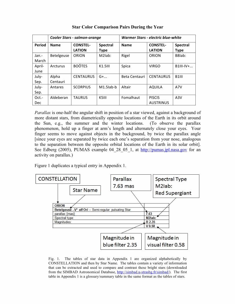
Star Color Comparison Pairs During the Year Cooler Stars -‐ salmon-‐orange Warmer Stars -‐ electric blue-‐white
Period Name CONSTEL-‐ LATION
Spectral Type
Name CONSTEL-‐LATION
Spectral Type
Jan.-‐March
Betelgeuse ORION M2Iab: Rigel ORION B8Iab:
April-‐June
Arcturus BOÖTES K1.5III Spica VIRGO B1III-‐IV+...
July-‐Sep.
Alpha Centauri
CENTAURUS G+... Beta Centauri CENTAURUS B1III
July-‐Sep.
Antares SCORPIUS M1.5Iab-‐b Altair AQUILA A7V
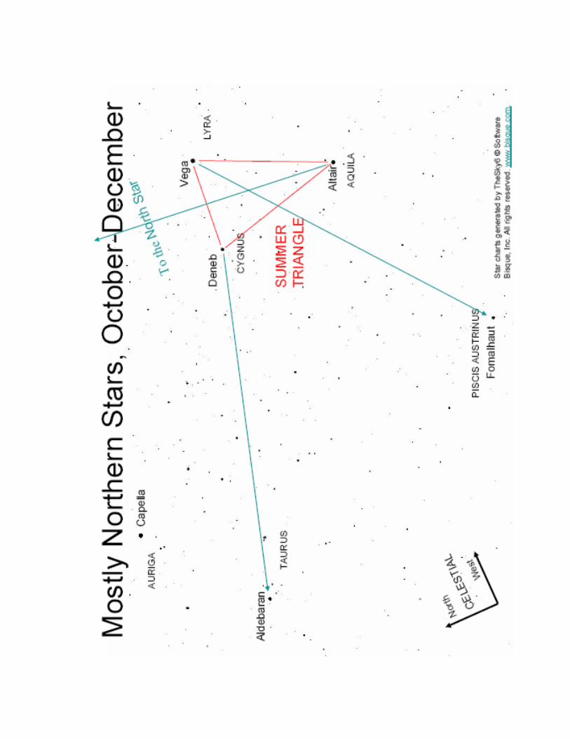
Oct.-‐Dec
Aldeberan TAURUS K5III Fomalhaut PISCIS AUSTRINUS
A3V
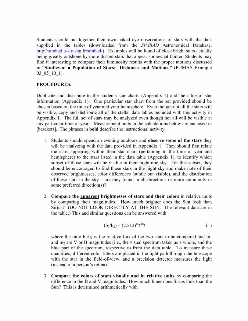
Parallax is one-half the angular shift in position of a star viewed, against a background of more distant stars, from diametrically opposite locations of the Earth in its orbit around the Sun, e.g., the summer and the winter locations. (To observe the parallax phenomenon, hold up a finger at arm’s length and alternately close your eyes. Your finger seems to move against objects in the background, by twice the parallax angle [since your eyes are separated by twice each one’s separation from your nose, analogous to the separation between the opposite orbital locations of the Earth in its solar orbit]. See Edberg (2005), PUMAS example 04_28_05_1, at http://pumas.jpl.nasa.gov for an activity on parallax.) Figure 1 duplicates a typical entry in Appendix 1.
Fig. 1. The tables of star data in Appendix 1 are organized alphabetically by CONSTELLATION and then by Star Name. The tables contain a variety of information that can be extracted and used to compare and contrast these bright stars (downloaded from the SIMBAD Astronomical Database, http://simbad.u-strasbg.fr/simbad/). The first table in Appendix 1 is a glossary/summary table in the same format as the tables of stars.

DISCUSSION: The following sets of stars can be used, and viewed, annually from either the northern or southern hemisphere, with considerable geographic and seasonal overlap. After choosing the time of year for observing, star selection should be based on any familiar constellations first and then biased toward the hemisphere in which you reside. Some stars will not be visible from the opposing hemisphere and others will barely skim the horizon. The quarters of the year used in the table are based on the assumption that the stars will be observed during evening hours. For viewing, there is considerable overlap of star availability across the quarterly boundaries (as with hemispheres) and they can often be seen for many months before the quarter given if the observer stays up later in the night or looks before dawn. Use a star chart, planisphere (“star wheel”), or planetarium software to determine which stars can be used to match the schedule of your syllabus. October through June (convenient for a typical school year in the northern hemisphere) offers a greater variety of star types (see “Spectral type” in the Appendix 1 tables), which will make the results more interesting.
Bright Evening Stars
Key: CONSTELLATION-‐Sky Hemisphere Star Name
Jan.-‐Feb.-‐Mar. Apr.-‐May-‐June July-‐Aug.-‐Sep. Oct.-‐Nov.-‐Dec. AURIGA – N Capella
AURIGA – N Capella
AQUILA – N Altair
AQUILA – N Altair
CANIS MAJOR – S Sirius
BOÖTES – N Arcturus
BOÖTES – N Arcturus
AURIGA – N Capella
CANIS MINOR – N Procyon
CANIS MINOR – N Procyon
CENTAURUS – S Alpha Centauri
CYGNUS – N Deneb
CARINA – S Canopus
CARINA – S Canopus
CENTAURUS – S Beta Centauri
ERIDANUS – S Achernar
ERIDANUS – S Achernar
CENTAURUS – S Alpha Centauri
CRUX – S Acrux
LYRA – N Vega
GEMINI – N Castor
CENTAURUS – S Beta Centauri
CRUX – S Mimosa
PISCIS AUSTRINUS – S Fomalhaut
GEMINI – N Pollux
CRUX – S Acrux
CRUX – S Gacrux
TAURUS – N Aldebaran
ORION – Equator Betelgeuse
CRUX – S Mimosa
CYGNUS – N Deneb
ORION – Equator Rigel
CRUX – S Gacrux
LYRA – N Vega
TAURUS – N Aldebaran
GEMINI – N Castor
PISCIS AUSTRINUS – S Fomalhaut
GEMINI – N Pollux
SCORPIUS – S Antares
LEO – N Regulus
VIRGO – Equator Spica
Students should put together their own naked eye observations of stars with the data supplied in the tables (downloaded from the SIMBAD Astronomical Database, http://simbad.u-strasbg.fr/simbad/). Examples will be found of close bright stars actually being greatly outshone by more distant stars that appear somewhat fainter. Students may find it interesting to compare their luminosity results with the proper motions discussed in “Studies of a Population of Stars: Distances and Motions,” (PUMAS Example 03_05_10_1). PROCEDURES: Duplicate and distribute to the students star charts (Appendix 2) and the table of star information (Appendix 1). One particular star chart from the set provided should be chosen based on the time of year and your hemisphere. Even though not all the stars will be visible, copy and distribute all of the stellar data tables included with this activity in Appendix 1. The full set of stars may be analyzed even though not all will be visible at any particular time of year. Measurement units in the calculations below are enclosed in [brackets]. The phrases in bold describe the instructional activity.
1. Students should spend an evening outdoors and observe some of the stars they
will be analyzing with the data provided in Appendix 1. They should first relate the stars appearing within their star chart (pertaining to the time of year and hemisphere) to the stars listed in the data table (Appendix 1), to identify which subset of those stars will be visible in their nighttime sky. For this subset, they should be encouraged to find those stars in the night sky and make note of their observed brightnesses, color differences (subtle but visible), and the distribution of these stars in the sky – are they found in all directions or more commonly in some preferred direction(s)?
2. Compare the apparent brightnesses of stars and their colors in relative units
by comparing their magnitudes. How much brighter does the Sun look than Sirius? (DO NOT LOOK DIRECTLY AT THE SUN. The relevant data are in the table.) This and similar questions can be answered with
(b1/b2) = (2.512)m2-m1 (1)
where the ratio b1/b2 is the relative flux of the two stars to be compared and m1 and m2 are V or B magnitudes (i.e., the visual spectrum taken as a whole, and the blue part of the spectrum, respectively) from the data table. To measure these quantities, different color filters are placed in the light path through the telescope with the star in the field-of-view, and a precision detector measures the light (instead of a person’s retina).
3. Compare the colors of stars visually and in relative units by comparing the
difference in the B and V magnitudes. How much bluer does Sirius look than the Sun? This is determined arithmetically with
Color Index (often shortened to “color”) = B – V (2) Which stars on the list are the most or least colorful? How do the calculations of color index compare with the students’ night sky observations of star colors?
4. Calculate the distances to stars. When an object is inaccessible – a far-away mountain summit or distant star – known distances can be combined with measured angles to determine the distance (and altitude for a mountain). The method relies on parallax (Edberg, 2005 for PUMAS example 04_28_05_1). The parallax (PLX) in milliarcseconds (thousandths of an angular second of arc, [mas]) can be converted from an angular measure to a physical distance (D) easily1. Multiply the parallax in [mas] by 1000 and then take the reciprocal:
D = 1/(PLX · 1000) [parsecs, pc] (3)
A parsec (parallax-second of arc) is the distance at which the angle
subtended by the radius of Earth’s orbit around the Sun, 1 astronomical unit (AU), is 1 arc second. To gain a feel for distances in parsecs, they can be converted to light years [ly], the distance light travels in one year’s time. Perhaps a comparison with a more familiar distance will help: One foot is about one billionth (10-9) of a light second and the distance from the Earth to the Sun is about 8 1/3 light minutes. A parsec is 3.261631 light years and a light year is 9.460536x10¹⁵ meters (Bishop, 2007):
1 [pc] = 3.262 [ly] (4)
Students should plot the stars’ distances on a graph’s x-axis and their V
magnitudes from Appendix 1 on the y-axis. Notice that with the exception of the Sun, all the stars have similar magnitudes (they were chosen because they are among the brightest in the sky), but one is much more distant, and the Sun appears very bright because it is very close.
5. Compare the true brightnesses of stars in relative units by comparing their
magnitudes and distances. The true brightness, called the absolute magnitude, is determined with
MV = V – 5log10D + 5 or (5a) MB = B – 5log10D + 5 (5b)
where D is the distance and V or B is the observed magnitude. The formulas scale the brightness of each star to the values they would have if they were all at
1 More advanced students may ask why trigonometric equations aren’t being used for these calculations, and some may notice that spherical trigonometry is really applicable. The answers are that for the tiny angles being discussed, the small angle approximation is applicable and treating the calculations as plane geometry will not reduce accuracy in any meaningful way for this activity.
the same distance, 10 parsecs, and the magnitude unit is retained for comparison2. How bright is the Sun actually, compared to these stars, if they were all at the same distance? How bright is Sirius, visually the brightest star in the sky, compared to some of the others? Use equation (1) and the absolute magnitudes from equations (5) for these comparisons. Plot the stars on a color-magnitude diagram (use the chart in Appendix 3). The stars in the data table of Appendix 1 can be plotted on a version of the original Hertzsprung-Russell diagram, named for astronomers Ejnar Hertzsprung and H. N. Russell, who first independently prepared plots of stellar absolute magnitude vs. spectral type. The horizontal axis should be color index (i.e., the difference between the Blue and Visual magnitudes, B-V), a surrogate measure for spectral type. The vertical axis is absolute magnitude (true brightness) MV per equation (5a). The stars plotted will generally fall on the upper portion of the diagram.
EXTENSION: Students should plot the stars’ distances on a graph’s x-axis and their absolute magnitudes on the y-axis. Notice that the stars’ absolute magnitudes pretty smoothly cover a wide range, and the brightest one is also the most distant (whereas the Sun is faintest and closest). Compare this plot with the magnitude vs. distance plot prepared in no. 3 above. Now introduce logarithms. Make two other plots by either plotting the distance on semi-log paper, or computing and plotting log10(distance) on cartesian graph paper. Distance is again on the x-axis with either V magnitude or absolute magnitude MV on the y-axes. The scattered MV values settle down into a fairly tight straight line on the absolute magnitude plot. This demonstrates the logarithmic nature of the magnitude system: the instructions in this paragraph use the log operation to generate the abscissa values. The ordinate values are logarithmic because that’s the way our eyes+brain judge differences in brightness – logarithmically, (2.512)m2-m1, and not linearly.
Taking in these investigations as a group, additional thought leads to the conclusions that (1) the brighter stars seen in the sky tend to be intrinsically brighter and they are more distant than much more numerous nearby, intrinsically fainter stars, and (2) brighter stars are much rarer, per unit volume, than fainter stars. REFERENCES: Bishop, R., 2008, “Some Astronomical and Physical Data” in Observer’s Handbook 2008, P. Kelly, ed., Royal Astronomical Society of Canada, Toronto. Edberg, S. J., 2005, “When A Ruler Is Too Short,” Practical Uses of Math and Science, an on-line refereed journal at http://pumas.jpl.nasa.gov , accepted 2005 August 25. 2 Aside from just distance, dust between stars can reduce the apparent brightness of a star, and if no correction is made, its absolute magnitude will be incorrect. The effect is negligible for this activity.
FOR MORE INFORMATION: Kelly, P., 2007, Observer’s Handbook 2008, Toronto: Royal Astronomical Society of Canada. Starry Nights Pro. (Ver. 3, 1997 was used; Ver. 6 is now available) [Computer software]. New York, New York: Imaginova. TheSky6 Professional Edition Version 6 for Windows. (2004). [Computer software]. Golden, Colorado: Software Bisque. http://www.astro.ljmu.ac.uk/courses/phys134/magcol.html http://www.astro-tom.com/technical_data/magnitude_scale.htm ACKNOWLEDGMENTS: I am grateful to Dr. Larry and Nancy Lebofsky, Dr. Ralph Kahn, and two anonymous reviewers for many fine edits and suggestions that improved the clarity and completeness of the discussions in this activity. This research has made use of the SIMBAD database, operated at CDS, Strasbourg, France, http://simbad.u-strasbg.fr/simbad/ . The star and constellation charts were generated by TheSky6 © Software Bisque, Inc. All rights reserved. www.bisque.com. The color-magnitude diagram is from Wikipedia, http://en.wikipedia.org/wiki/Main_sequence, where a color version may be found. This publication was prepared by the Jet Propulsion Laboratory, California Institute of Technology, under a contract with the National Aeronautics and Space Administration. Reference herein to any specific commercial product, process, or service by trade name, trademark, manufacturer, or otherwise, does not constitute or imply its endorsement by the United States Government or the Jet Propulsion Laboratory, California Institute of Technology.
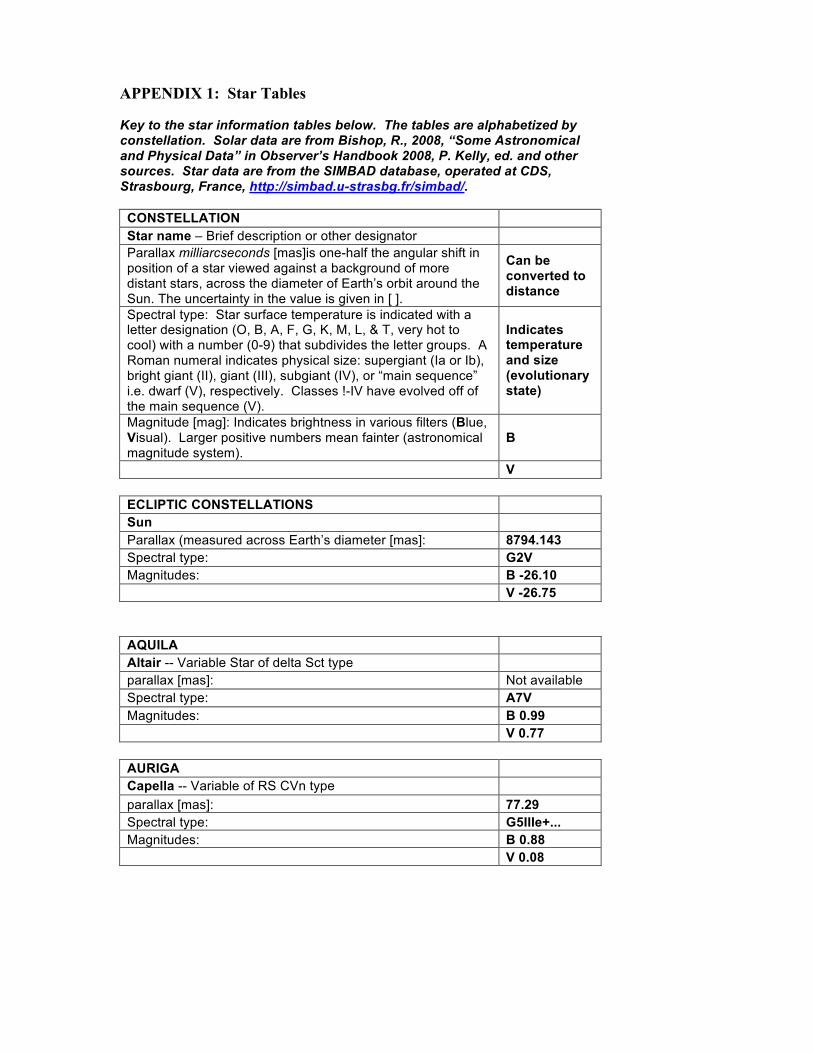
APPENDIX 1: Star Tables Key to the star information tables below. The tables are alphabetized by constellation. Solar data are from Bishop, R., 2008, “Some Astronomical and Physical Data” in Observer’s Handbook 2008, P. Kelly, ed. and other sources. Star data are from the SIMBAD database, operated at CDS, Strasbourg, France, http://simbad.u-strasbg.fr/simbad/. CONSTELLATION Star name – Brief description or other designator Parallax milliarcseconds [mas]is one-half the angular shift in position of a star viewed against a background of more distant stars, across the diameter of Earth’s orbit around the Sun. The uncertainty in the value is given in [ ].
Can be converted to distance
Spectral type: Star surface temperature is indicated with a letter designation (O, B, A, F, G, K, M, L, & T, very hot to cool) with a number (0-9) that subdivides the letter groups. A Roman numeral indicates physical size: supergiant (Ia or Ib), bright giant (II), giant (III), subgiant (IV), or “main sequence” i.e. dwarf (V), respectively. Classes !-IV have evolved off of the main sequence (V).
Indicates temperature and size (evolutionary state)
Magnitude [mag]: Indicates brightness in various filters (Blue, Visual). Larger positive numbers mean fainter (astronomical magnitude system).
B
V ECLIPTIC CONSTELLATIONS Sun Parallax (measured across Earth’s diameter [mas]: 8794.143 Spectral type: G2V Magnitudes: B -26.10 V -26.75 AQUILA Altair -- Variable Star of delta Sct type parallax [mas]: Not available Spectral type: A7V Magnitudes: B 0.99 V 0.77 AURIGA Capella -- Variable of RS CVn type parallax [mas]: 77.29 Spectral type: G5IIIe+... Magnitudes: B 0.88 V 0.08

BOÖTES Arcturus -- Variable Star parallax [mas]: 88.85 Spectral type: K1.5III Magnitudes: B 1.19 V -0.04 CANIS MINOR Procyon -- Spectroscopic binary parallax [mas]: 285.93 Spectral type: F5IV-V Magnitudes: B 0.74 V 0.34 CANIS MAJOR Sirius -- Spectroscopic binary parallax [mas]: 379.21 Spectral type: A1V Magnitudes: B -1.46 V -1.47 CARINA Canopus -- Star parallax [mas]: 10.43 Spectral type: F0II Magnitudes: B -0.57 V -0.72 CENTAURUS Alpha Centauri -- Double or multiple star parallax [mas]: 742 Spectral type: G+... Magnitudes: B 0.4 V -0.1 CENTAURUS Beta Centauri -- Variable Star of beta Cep type parallax [mas]: 6.21 Spectral type: B1III Magnitudes: B 0.38 V 0.60 CRUX Acrux -- Spectroscopic binary parallax [mas]: Not available Spectral type: B0.5IV Magnitudes: B 1.32 V 1.4
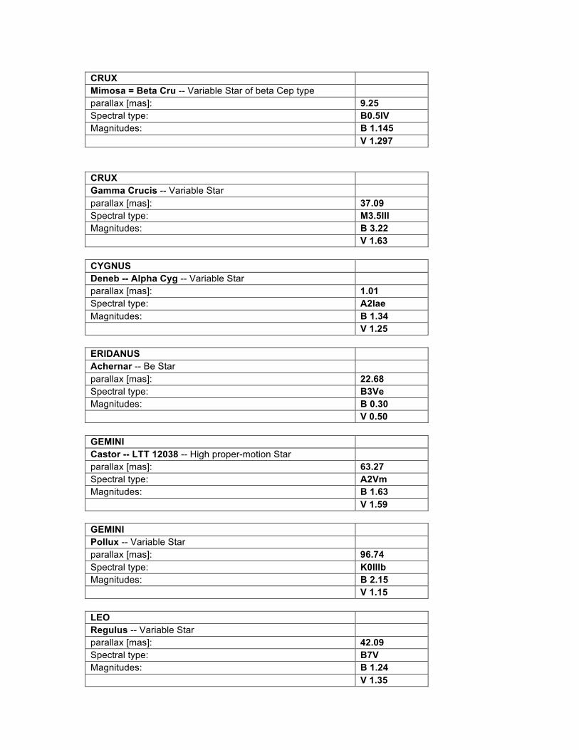
CRUX Mimosa = Beta Cru -- Variable Star of beta Cep type parallax [mas]: 9.25 Spectral type: B0.5IV Magnitudes: B 1.145 V 1.297 CRUX Gamma Crucis -- Variable Star parallax [mas]: 37.09 Spectral type: M3.5III Magnitudes: B 3.22 V 1.63 CYGNUS Deneb -- Alpha Cyg -- Variable Star parallax [mas]: 1.01 Spectral type: A2Iae Magnitudes: B 1.34 V 1.25 ERIDANUS Achernar -- Be Star parallax [mas]: 22.68 Spectral type: B3Ve Magnitudes: B 0.30 V 0.50 GEMINI Castor -- LTT 12038 -- High proper-motion Star parallax [mas]: 63.27 Spectral type: A2Vm Magnitudes: B 1.63 V 1.59 GEMINI Pollux -- Variable Star parallax [mas]: 96.74 Spectral type: K0IIIb Magnitudes: B 2.15 V 1.15 LEO Regulus -- Variable Star parallax [mas]: 42.09 Spectral type: B7V Magnitudes: B 1.24 V 1.35

LYRA Vega -- Alpha Lyr -- Variable Star parallax [mas]: 128.93 Spectral type: A0V Magnitudes: B 0.03 V 0.03 ORION Betelgeuse --V* alf Ori -- Semi-regular pulsating Star parallax [mas]: 7.63 Spectral type: M2Iab: Magnitudes: B 2.35 V 0.58 ORION Rigel -- Emission-line Star parallax [mas]: 4.22 Spectral type: B8Iab: Magnitudes: B 0.09 V 0.12 PISCIS AUSTRINUS Fomalhaut -- Variable Star parallax [mas]: 130.08 Spectral type: A3V Magnitudes: B 1.25 V 1.16 SCORPIUS Antares -- Alpha Sco -- Semi-regular pulsating Star parallax [mas]: 5.40 Spectral type: M1.5Iab-b Magnitudes: B 2.96 V 1.09 TAURUS Aldebaran -- Alpha Tau -- Variable Star parallax [mas]: 50.09 Spectral type: K5III Magnitudes: B 2.39 V 0.85 VIRGO Spica -- 67 Vir -- Variable Star of beta Cep type parallax [mas]: 12.44 Spectral type: B1III-IV+... Magnitudes: B 0.91 V 1.04
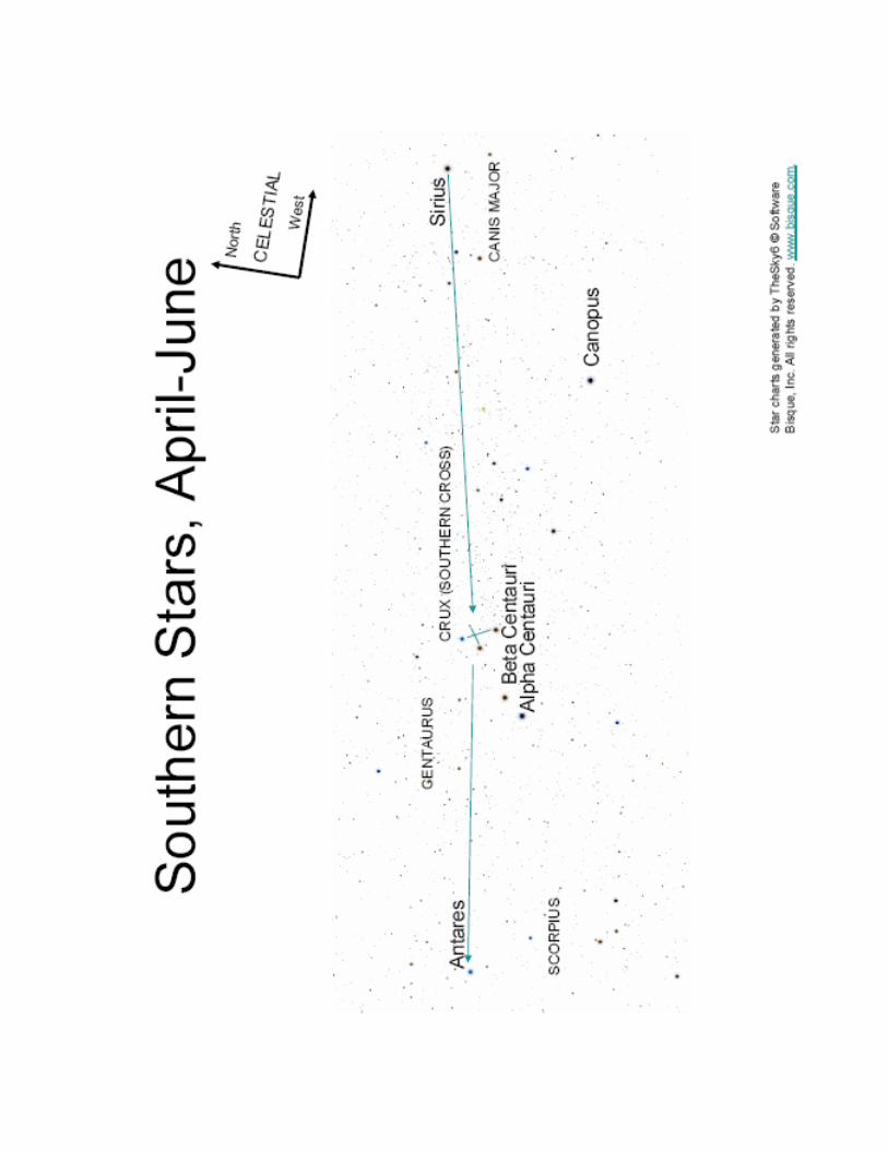
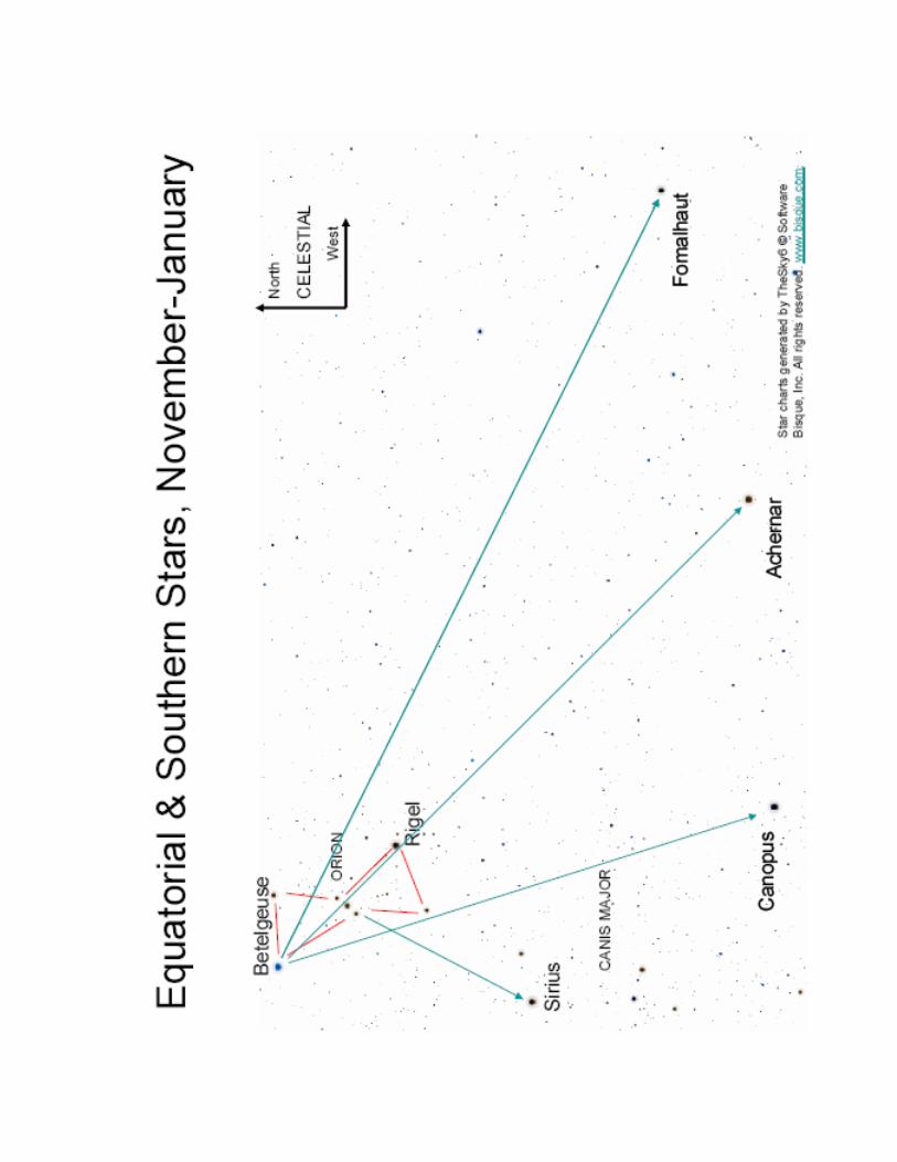
APPENDIX 2: Star and Constellation Charts
The following collection of charts is designed to make it easy to find and identify bright stars. In the charts, prominent and/or well-known stars or groups of stars, constellations, or super-constellations are used to point to other prominent stars. If desired, once a prominent star is found, other charts can be used to identify other stars in a constellation until the full constellation is recognized.
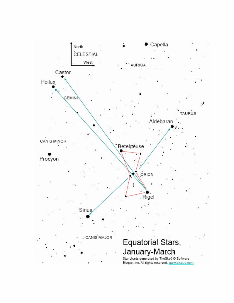
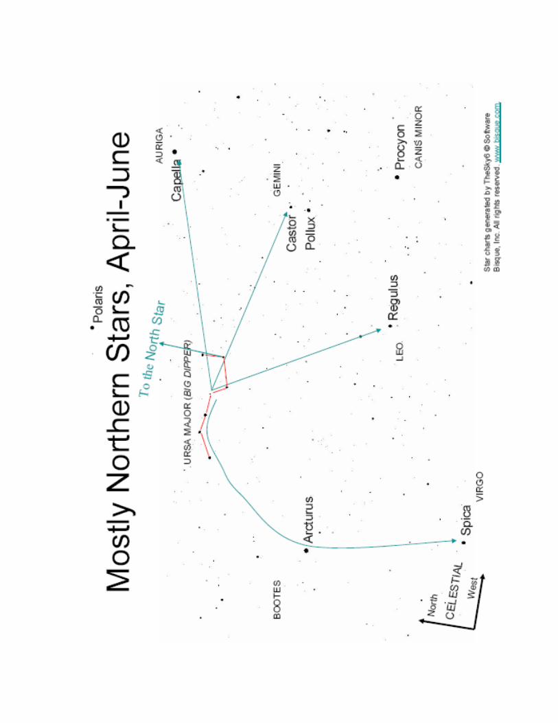
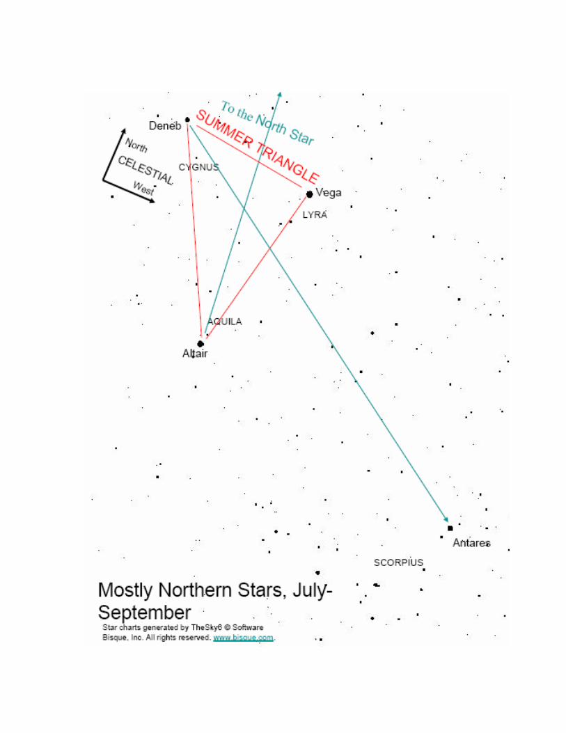
These charts are useful over large areas of Earth’s northern and southern hemispheres. They place a significant fraction of a celestial hemisphere on a small, flat piece of paper; sometimes stars or constellations will be below the horizon or blocked by local landmarks. Use separations between recognized stars (especially those paired) to make “pointers” to gauge the distance to the desired target star. In the northern hemisphere, April-June, the BIG DIPPER asterism (part of the constellation URSA MAJOR) visible high in the north is particularly good for learning the sky. ORION is good from November-January in the southern hemisphere and January-March in the northern hemisphere. Though the charts are labeled to indicate a hemisphere, many of the stars will be visible from the opposing hemisphere, depending on your latitude.
As a general rule, facing south is best, but some neck-craning (and/or facing a different direction and rotating the chart) will be necessary to go from the starting point to the target stars at the ends of the arrows. The font convention for the charts is that CONSTELLATIONS are fully capitalized and Star Names are larger and first-letter capitalized. Celestial North and West refer to the direction to those points on the horizon as seen on the sky. (In other words, east and west on the sky and on the charts are reversed compared to maps of features on Earth.) Most important: Choose a familiar group of stars, recognizable on a chart, and “star hop” from there.
The orientation “rose” in the lower left of the star charts can help with using the charts at night. At night, some observers find it is easier to use printed star charts with black stars on a white background rather than white stars on a black background. Black on white saves copier toner as well. The charts can be copied from this document and easily reversed with your image viewing and manipulation software if desired. These star charts were generated by TheSky6 © Software Bisque, Inc. All rights reserved. www.bisque.com.
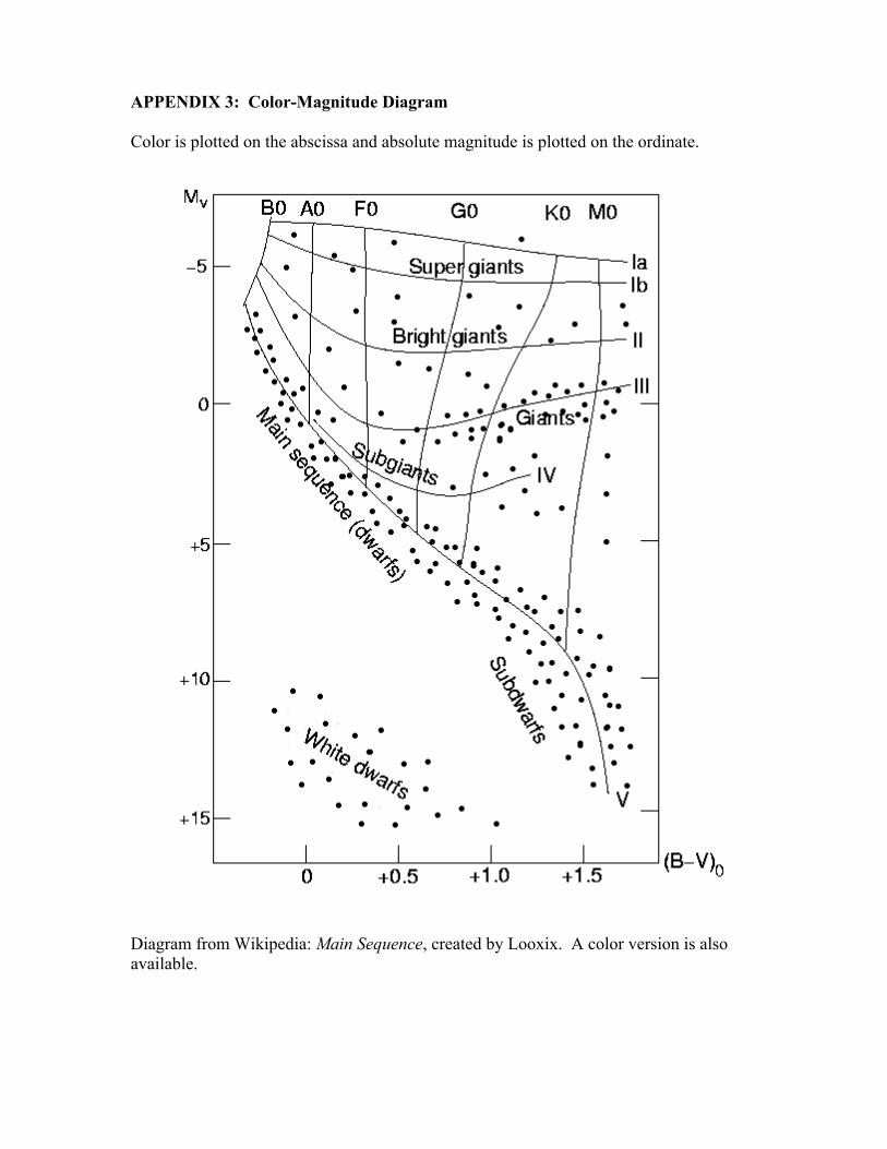
APPENDIX 3: Color-Magnitude Diagram Color is plotted on the abscissa and absolute magnitude is plotted on the ordinate.
Diagram from Wikipedia: Main Sequence, created by Looxix. A color version is also available.