NASA Contractor Report 3051

Studies of Convection in a Solidifying System With Surface Tension at Reduced Gravity

Basil N. Antar and Frank G. Collins

CONTRACT NASS-32484 SEPTEMBER 1978

nJAsA

https://ntrs.nasa.gov/search.jsp?R=19780024443 2018-05-12T23:26:31+00:00Z

TECH LIBRARY KAFB, NM

NASA Contractor Report 3051

Studies of Convection in a Solidifying System With Surface Tension at Reduced Gravity

Basil N. Antar and Frank G. Collins The University of Tetznessee Space Institute Tullahoma, Tennessee

Prepared for George C. Marshall Space Flight Center under Contract NASS-32484

National Aeronautics and Space Administration

Scientific and Technical Information Office

1978

FOREWORD

The research reported herein was supported by NASA contract NAS8-32484. Dr. George H. Fichtl and Mr. Charles Schafer of the Atmospheric Sciences Division, Space Sciences Laboratory, Marshall Space Flight Center, were the scientific monitors; and support was provided by the Office of Applications, NASA Headquarters.

g? .

TABLE OF CONTENTS

I INTRODUCTION

II MATHEMATICAL FORMULATION

III NON-DIMENSIONAL PARAMETERS

IV DISCUSSION

V CONCLUSIONS

References

Figures

Tables

Appendix I

Appendix II

Appendix III

. . . 111

Page

1

4

25

30

35

36

38

51

57

60

61

1. Introduction

One of the principal objectives in the future utilization of

orbital laboratories and stations is the production of materials

in space. This type of material production is referred to as space

processing. One of the primary constituents of most production process.es

involves the solidification of materials. The broad objective of the

present report is to investigate the solidification process in a low

gravity environment, while the specific task is to look at the stability

of the solid-liquid interface under the same conditiuns. The meaning

of the term stability as used here will be discussed more fully later

on in the report.

The problem of material solidification in general has attracted

researchers for many decades due to both its importance to industry

from the practical point of view and its mathematical difficulty from

the theoretical point of view. The analytical solidification problem

is commonly known as the "Stefan Problem" in honor of Jakob Stefan

(1889), who first formulated it. At the present time, solutions to

various aspects of the problem exist under different boundary condi-

tions, such as to make it of practical use for industrial applications.

For recent reviews of such solutions the reader is referred to the

books by Rubinstein (1971) and Ockendon and Hodgkins (1975). Also,

the not-so-recent review articles by Boley (1969) and Muehlbauer and

Sunderland (1965) are informative. However, the problem in its entirety

is far from solved,as is revealed from a scan of the recent literature

which, incidentally, also shows the continued interest in Lhe problem.

The mathematical difficulty of the problem is manifested in the

fact that although the governing equations are linear, the boundary

conditions are strongly non-linear, with the added difficulty that

the boundaries are not stationary. Due to this second complication,

almost all of the solutions to the problem are time dependent with

only very few exceptions where it is steady.

Careful inspection of the problem reveals that the formulation

of the problem is not at all altered when the surrounding environment

is at reduced gravity. Hence, all of th:e mathematical difficulties

alluded to earlier are present under the new conditions. However,

instead of tackling the full-blown problem for the present report

and thus adding relatively little new information, it was decided

to look at one aspect of the problem which might be of relevance to

space processing. This aspect involves the deformation of the solid-

liquid interface from its original form during a solidification process

in a reduced gravity environment.

The problem just defined above is not unique to space process-

ing, and there exist quite a few applications for ground base work.

If the solidifying material is composed of a binary alloy, for example,

it has been shown first by Mullins and Sekerka (1964) and later by

Wolkind and Segel (1970) that the solid-liquid interface could deviate

from its original planar configuration for both finite and infinitesimal

disturbances. On the other hand, if the solidification process is

allowed to proceed from the upper boundary of the liquid, instabilities

of the Benard type might contribute to the deformation of the

phase boundary. Such a problem has been investigated by many workers,

some of whom are Turcotte (1974), Schubert et al. (1975), and Busse

2

and Schubert (1971), where the application was to mantle convection.

Also, the same type of instabilities might set in during a melting

process if the melting is from below, as is shown analytically by

Sparrow et al. (1977) and later verified experimentally also by Sparrow

et al. (1978).

In the present report the stability of the solid-liquid interface

of a pure metal will be studied during a solidification process in

which the liquid surface is free. Two such problems will be considered,

one in which the phase boundary is ftationary and another in which it

is propagating at a constant speed. Note that the added complication

due to the solidification of a mixture or a binary alloy is avoided

here since it will not greatly enhance the basic understanding of the

problem. Since the problem will be analyzed in a zero gravity environ-

ment, buoyancy effects do not contribute to the problem, thus leaving

only the influence of a variable surface tension to be investigated.

Seki et al. (1977) have studied the influence of surface tension

coupled with buoyancy effects on the stability of the phase boundary.

Their work, however, relates to a stationary phase boundary. Chang

and Wilcox (1976), on the other hand, considered the effects of surface

tension in a floating zone melting process. However, their analysis

was not of the stability type but rather numerical in which the

solidification process does not enter.

In the next few sections of this report the problem to be studied

will be defined and the equations will be set up with the appropriate

boundary conditions. Then the problem will be solved and the results

tabulated and discussed. In the, final section these results will be

discussed as they apply to real worki,ng materials such as some pure

metals whose use is anticipated in space processing applications.

3

2. Mathematical Formulation

The complete analysis of the shape of the solid-liquid interface

in a general solidification process is extremely complicated, which

ultimately might require a complicated numerical solution and thus

is beyond the scope of the present report. Alternatively; it is

possible to study the stability of the interface for a simple geo-

metrical configuration. By stability'of the interface the question

is asked: given an original shape of the interface, say, planar, or

any other configuration, under what conditions will the shape remain

unaltered during the various stages of the solidification process?

This is a typical example of a classical hydrodynamic stability problem

in which it is determined whether the interface geometry will change

if a slight disturbance is imposed on the original configuration.

The evolution of this disturbance with time wi17 then determine the

fate of the original configuration. If the disturbance decays with

time, then the original configuration is said to be stable with respect

to the disturbance, and it is unstable otherwise. If the disturbance

is infinitesimal, then the stability analysis is called linear, and if

it is finite then the analysis is nonlinear. In the present report,

only linear stability analysis will be performed.

Since most stability analyses are performed with respect to time,

it is imperative that an original state is found which is either

independent of, orat most periodic with, time. As discussed in the

introduction, in a solidification process the solution is almost

always a nonperiodic function of time. For the present study two

solutions for the mean state were found which are independent of time,

both of which are analyzed here. The first configuration which is shown

in Figure 1 constitutes a fluid and a solid layer which are in equilib-

rium and hence the liquid-solid interface is planar and stationary.

Although such a configuration is not strictly a solidification process

it is nevertheless used for illustrative purposes and further to

unravel the main difficulties associated with the problem. The second

configuration constitutes a continuous solidification process in which

the interface boundary is moving at a constant rate. Vi th a simple

transformation it will be shown that a steady state solution exists

for this process, thus facilitating a managable linear stability

analysis. This second example is closer to a real solidification

process and thus is a more realistic example than the first.

Since the present stability analyses are linear, a direct answer

to the stability of the interface cannot be obtained. The stability

or the instability of the interface will be considered as a conse-

quence of the stability or instability of the fluid. Thus, if the

analysis reveals the liquid to be unstable to infinitesimal distur-

bances, it is then assumed that convection of some sort will set in

the liquid in such a way as to disturb the original shape of the

interface and probably deform it, as shown schematically in Figure 2.

If the fluid is found to be stable, on the other hand, it will be

assumed that any initial deformation of the interface will be evened

out and the interface will retain its original configuration.

2 .l Steady State Solidification Process

A. The Mean State Solution

It can be formally proven, and will be shown below, that if the

upper surface of a melt layer which is on top of a solid layer whose

surfaces are kept at a constant but different temperature .each, then

part of the melt will solidify until the solid-liquid interface reaches

an equilibrium position. This equilibrium position of the solid-

liquid interface is a function of both temperatures and the solidifica-

tion temperature only. This is one of the basic and simple steady

state solutions to the Stefan problem [Rubinstein (1971)]. As a first

example, the stability of this solution will be studied where a sketch

of the problem is provided in Figure 1.

Consider two finite depth layers, one of melt and another of

solid, which are infinite in the horizontal direction, where the

temperature distribution in both the liquid and solid is denoted by

TX and Ts, respectively. Since there is no convection in the mean

state, the energy equations for a steady state are given by

with the temperature at the top of the liquid layer given by

Tia(d)=Ti and the temperature at the bottom of the solid is given by

T;$O)=T;. In here the asterisk denotes dimensional quantities.

However, since we are considering a solidification process, the energy

balance and conservation of mass considerations at the solid-liquid

interface imposes the following three additional cond itions . .

I ip = s

6

where ks and kit are the thermal condictivities of the solid and liquid,

respectively. Trf; is the solidification temperature and S is the

equilibrium position of the interface.

A solution to equation (1) with all the boundary conditions is

given by

where

(3)

The equilibrium position of the interface is uniquely determined by

this solution to be

where .

The so lution gi ven by (3) is identical to that obtained by Rubinstein

(1971) for the time dependent problem in the limit as time+,. Further-

more, the above solution is no more than the steady conduction solution

for the fluid and solid layers with a linear temperature distribution

in each.

(4)

I

B. Linear Stability Analysis

In order to investigate whether the interface boundary can withstand

as light perturbation, a linear stability analysis was performed on

the mean state solutions (3) and the boundary conditions. The analysis

was carried out along lines which are similar to what is commonly done

in hydrodynamic stability analyses. The field variables are first

decomposed into a mean and a perturbation in the form

75.z +7-‘, ; = iTo +Z’ > (5)

where T is the temperature field and: is the velocity vector. Z. in

the present case is zero since it is assumed that there is no convective

motion in the mean state. These f 'unctions are then substituted into

the momentum and energy equations and the mean state is subtracted

out. Since we are considering on1 y a linear stability analysis, the

remaining equations for the perturbation functions are then linearized.

Furthermore, these equations are then manipulated to eliminate the

pressure term resulting in the following equations:

(6)

(7)

(8)

I’

Use has been made in the above equations of the mass conservation

equation. In these equations v is the kinematic viscosity of the

liquid, K$ and K~ are the thermal diffusivities of the liquid and

solid, respectively, and W’ is the z component of the velocity vector,

'and d T OR is the temperature gradient of the mean state in the liquid dz

which is a constant in this case. The independent variables in equa-

'tions (6)-(8) have been made dimensionless in the following way.:

.( x, 's , t ) = ( d'cl , y' Id a t*/d ) >

t = t*4/d= 1

LJ.’ = w”d/Ht 0

7 = (9)

and

where again the asterisk indicates dimensional quantities.

The set (6)-(8) constitutes a linear partial differential system

for the perturbation variables w', T; and Tk. A solution to this set

is sought for appropriate boundary conditions which are obtained in the

following way. At the lower surface of the solid it is assumed that

the temperature perturbation is zero, i.e.,

7y10) = 0

At the top of the surface of the liquid we require the velocity

perturbation to be also zero, i.e.,

(10)

tJ *‘(d+s) = 0

9

Also, a radiation condition is imposed on the upper surface of the

liquid in the form

where q represents the rate of change with temperature of the rate of

loss of heat per unit area from the upper surface to its upper environ-

ment. Note if q-ta we approach a conducting boundary condition, while

if q-+0 we approach an insulating boundary condition. A comprehensive

discussion of this boundary condition is provided by Pearson (1958).

Another condition to be imposed on the upper surface of the liquid

layer is that of the balance of the tangential forces on that surface,

which is given by Levich and Krylov (1969):

where CT and p are the surface tension and dynamic viscosity of the fluid.

Now, since the surface tension is known to be a strong function

of temperature, the above condition will be valid only if the tempera-

ture of the upper surface is not constant. If instabilities will set

in the fluid, the temperature distribution will not be constant on the

surface and the surface tension force will play a major role in the

stability analysis. For the purpose of the present report it will be

assumed that the surface tension is a linear function of temperature

in the form

G = Go + id,

10

au where b = x and a0 is a constant. With this approximation the OR

condition for the balance of the tangential forces may be rewritten as:

“(g2 +a* aya ) 7”: b (& +$,2 -$)fl* * @ t = S+d. (13)

There remains the boundary conditions at the interface to be

satisfied. The first is the requirement that the temperature at the

interface regardless of the position of the interface remains the

solidification temperature leading to

Here it is assumed that the perturbed position of the interface to a

first order of approximation is the same as its unperturbed position.

Also, at this position, where the solid boundary acts as a wall, the

no-slip conditions are imposed and take the form

a/‘, 0 32’

@Z-S,

while the linearized form of the energy balance at the interface leads

to

(14)

(15)

where p, is the density of the solid and L is the latent heat of fusion

Condition (16) is not intuitively obvious and is rigorously derived

in Appendix 1 for the present case and for the subsequent case also.

The linear system of equations (6)-(7) together with the separable

linear boundary conditions (lo)-(16) admit solutions through the

11

separation of variables method. To obtain such a soluti on the perturba-

tion variables must take the following functional form:

[ I

(17)

Note that only a two-dimensional form of the perturbation function is

considered, where it is hoped that the analysis is not affected in a

major way.

Substituting (17) into (6)-(7) leads to the following system of

ordinary differential equations for the perturbation functions

The question of stability or instability can be settled by deter-

mining the value of ao. Specifically, only the sign of Re(a,) is needed

since if Re(ao) is negative, zero or positive then the system is stable,

neutral or unstable, respectively. To even determine the sign of Re(ao)

is quite tedious and instead the principle of exchange of stability is

invoked here. This principle implies that if Re(ao)=O then Im(ao)=O

and if this is true, then it is possible to set ao=O in order to deter-

mine the neutral stability criteria. Adopting this principle reduces

the system of equations to the following:

(18)

12

(b’-a’)tPs = 0

while the boundary conditions will take the following form:

where

In the above boundary conditions the origin has been shifted to the

interface boundary.

The solutions to equations (20) and (21) may be written immedi-

ately in the form

13

(20)

(21)

(22)

C-23)

(24)

Satisfying the boundary conditions for the perturbation temperature

in the solid leads to

and thus

&: s 0 . (25)

However, A, through AS may be determined from the conditions on the

perturbation temperature in the liquid. Since we are looking for

neutral stability curves the exact values of Ai need not be determined

but if all the conditions are to be satisfied and since the conditions

are homogenous, the requirement that the coefficients be unique will

lead to the following parameter relation:

where D,, D2 and DS are the following determinants:

14

L

This equation gives the required relationship between the Marangoni

number and the wave number of the neutrally stable disturbances.

2.2 Constant Rate Solidification Process

A. The Mean State Solutions

The analysis performed in the previous section was for a stationary

interface in which the solidi.fication process entered only in the per-

turbation equations and not in the mean solution. Thus, the example

does not realistically model a solidification process and was used

only for the simplicity of the mathematics involved and for illustra-

tive purposes. In this section the analysis of a more realistic

15

problem is presented. The problem will involve a continuous solidifica-

tion process in which the melt is being fed continuously and at a

constant rate while the solidification rate is proceeding also at a

constant rate. A sketch of the problem is shown in Figure 3. However,

in order to keep the solidification rate constant for a continuous

process, it is required that the heat removal rate at the bottom of

the solid be also constant. The physical analog of this model could

be a continuous solidification process in which the melt is being

replenished all the time in an exact amount to keep its mass constant

for a very slow solidification process.

Thus, consider a finite depth melt which is infin-ite in the hori-

zontal extent on top of a solid layer. The temperature distributions

in both the solid and the liquid are given by the one-dimensional energy

equations [Carslaw and Jaeger (1959)] in the form

where p, and pR are the densities of the solid and liquid, respectively,

and the rest of the notation is the same as that used in the previous

section. Note that here the interface position S(t) is a function

of time and not a constant as before. However, it will be assumed from

the start that the interface moves at a constant speed v P'

where

(30)

(31)

16

(32)

At this point, as will prove beneficial later, the origin of the

coordinates is moved to the solid-liquid interface via the following

G.allelain transformation:

This transformation will render equations (30) and (31) to the

following form:

Also in these equations the primes have been dropped for ease of notation.

The boundary conditions appropriate to this problem- are the following:

(33)

(34)

(35)

1.36)

(37)

(38)

Note that for the solid boundary condition a heat transfer rate condition

is used rather than a fixed temperature condition in order to be

consistent with the assumption of a constant solidification rate.

The temperature distribution in the liquid phase may be obtained

from the solution of the above system to be:

t-391

where T oR and z are d imensionless quantities having the followi,ng form:

A plot of this distribution of temperature is given in Figure 4. The

system of equations and the boundary conditions also specify uniquely

the temperature distribution in the solid and the propagation speed

of the interface. However, use will be made of the latter condition

which is also a matching condition and will be written out when the

need arises.

B. Linear Stability Analysis

As indicated earlier, the stability of the solid-liquid interface

is inferred from the stability of the liquid phase. The stability

analysis here is performed in a very similar manner as was done in

the previous section. Again, the temperature and velocity fields are

separated into a mean and a perturbation and substituted into the

momentum and energy equations resulting in a linearized form for the

equations for the perturbation functions. In this case, however,

18

a Gallehian transformation is ,again adopted as was done for the mean

temperature distribution where w '

t =t* WI

x r sin

Also, the resulting independent variables in the new frame of reference

are non-dimensionalized in the following way:

L “,q,t 1 = L x;J > Y*/d d’ld 1 z = ?/L$

where d is the depth of the liquid layer.

The resulting linear non-dimensional governing equations for the

perturbation functions are

Most boundary condit ions under which the above equations are to be

solved in the moving frame of reference are identical to conditions (.lO)-

(16) except for cond ition (16) which now is given by

(40)

(41)

(42)

19

Again, due to the form.of the boundary conditions, equations (40)-

(42) may be solved through the normal mode method. It will be assumed

for simplicity that the perturbation functions are two-dimensional.

Under these circumstances the perturbation functions will take the

same form as (17). Substituting this functional form of the solution

into equations (40)-(42) we get after setting a, = 0:

where

R= @/d

(43)

(44)

(45)

In equations (43)-(45) we have again invoked the principle of excha.nge

of stability.

The solution method for the system of equations (43)-(45) is

slightly different here from that of the previous case. First,

20

equation (43) is solved alone for the velocity perturbation v(z).

Then equation (44) is solved for the temperature perturbation O&Z)

as an inhomogenous equation. Equation (45), however, is uncoupled

and may be solved

easily written in

separately. The solution for equation (43) may be

the form r(

where Xi are given by

‘x -+a r,t - (47)

‘x ‘i,q = - +p+f (q$+dp

while the solution to equation (44) is given by

4 c

$W = L' is1

A; C; Q+S, +-x;h\ -t c

i fl,*pIa;t)

i= C (481,

where Al through A4 and Xl through X4 are the same constants as those

in the velocity distribution, while X5 and X6 are given by

(46)

1 C,b =-

The Ci appearing in (48) are given by

(49)

21

where

x, = Wp

Since the solution for the perturbation velocity and temperature are

obtained separately it is instructive to give the boundary conditions

Thus substituting the solutions given by (46) and (48) into the boundary

conditions (52) yields a system of equations for A. If the value of

the coefficients Ai is to be unique then the determinant of the coeffi-

cient matrix for Ai must be zero, i.e.,

(51)

(52)

.det Lq = o

where the matrix E is given .by

22

(54)

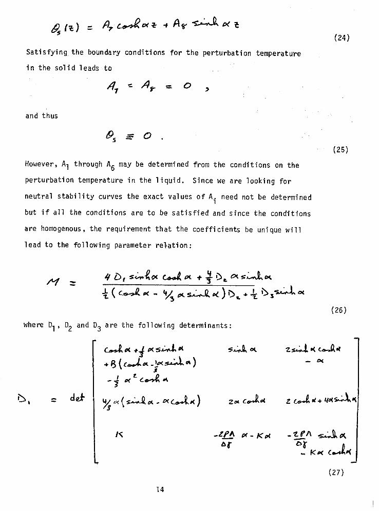
To obtain the neutral stability curves equation (54) is then solved for

one of the parameters in terms of the rest, i.e.,

t.56 >

24

3. Non-Dimensional Parameters

The goal of the present work is to calculate the neutral

stability curves and the critical Marangoni number, M, as a

function of the non-dimensional wave number .of the disturbance.

It was necessary to non-dimensionalize the problems to be able

to make these calculations. There are always many ways to

non-dimensionalize a problem, but the method used recover

familiar dimensionless parameters plus additional parameters.

3.1. Steady State Process

The dimensionless independent variables were defined along

with the solution to the problem given earlier. The dependent

variables were non-dimensionalized to give the following relation-

ship for the neutral stability curve:

M= M(a,B,A,y,A, 0

where , da dTb'il

M=dT"p-d 2

a =dk=F= dimensionless wave number (A = disturbance wave length, k = disturbance wave number)

B=S! kll

= Biot modulus

A= L Cps(T;-T;)

dTOR

'= dz

25

K = kR/ks

It was desirable to calculate the neutral stability curves

using values of these parameters which characterize material

systems of interest for space processing. Table I lists property

values for some metallic materials that would be of interest.

The parameters A and K depend only upon the material properties

and their values are tabulated in Table II. A varies from 0.7

to 3.0 for the metals considered, while K varies from 0.44

to 1.74 but.is generally around 0.5.

The remaining dimensionless parameters depend upon the

boundary conditions of the problem as well as the material

properties. First consider the mean temperature field. The

analysis assumed that the material pr'operties were constant

but in fact they are strong functions of temperature. There-

fore, for this reason and because solidification usually

proceeds slowly, the temperature difference across the liquid-

solid system can be assumed to be small, say, 2°C. Then A

varies from 35 to 200 and y from 1.2 to 1.5, Jc

The Biot modules,

B, on the other hand, which characterizes the heat transfer

through the upper liquid surface, can be left as a parameter

in the problem.

%maller values of A correspond to large values of (TS-TI) and cannot be expected to yeild satisfactory results using the present analysis.

26

1;

3.2. Constant Rate Process

For the continuous rate process the neutral stability

curve is given by the following relation:

M = M(a,R,Pr,Q,B,A,K,P,C)

. where vPd = Reynolds number

R=- %

% Pr = - = Prandtl number 5L

P= pdpS

c = cp /c

0 ,., pS

Q = qos d,

kg U2-T,>

A= L J Cp (T;-T;)

S

and K and B are defined as before. Notice that A is now ;k

defined in terms of T2 -T" and is thus different from the parameter m

defined for the steady state problem. M is defined as

If a mean temperature gradient in the liquid defined by

* Jc dcs M=

(T2-Tm) do”

VP

1 1 dT* =

(T~-T;) 7 dz d

27

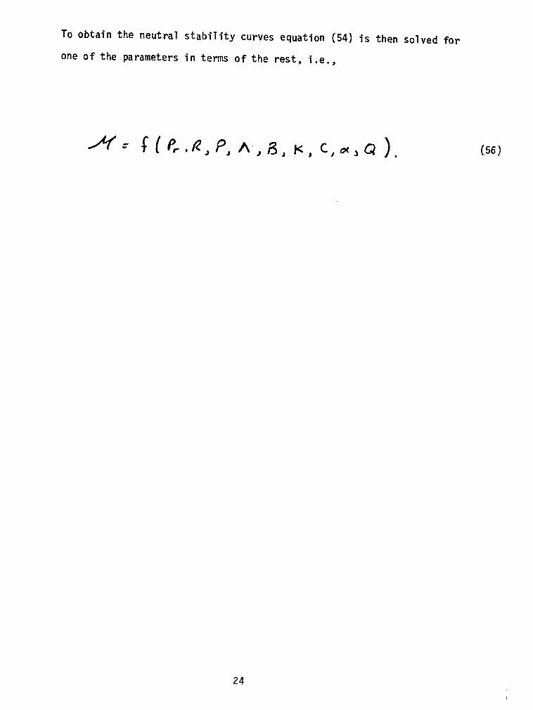
is used in the definition of the Marangoni number, then M

is related to it as follows:

M= R Pr M

However, M is the more natural parameter for the analysis and

the neutral stability curves will be given in terms of it.

Since Pr is small M is considerably smaller than M, for

Reynolds numbers of the order of one.

The continuous rate problem was non-dimensionalized using

the-speed of the phase plane, v P'

as one of the parameters in

(M and R). The phase plane speed is not one of the boundary

conditions of the problem but rather is part of the solution.

It is determined from the non-linear matching condition that

results from matching the solutions at the liquid-solid

interface for the mean motion. That matching condition is the

following:

0 OS

This relation can be non-dimensionalized using the parameters

listed above and they were selected, in part, to accomplish that

non-dimensionalization. In non-dimensional form the equation

becomes

QPC AR fr

From Table II it can be seen that Pr = p(10W2), A=O(l), and

P = O(1). Therefore, the exponentials are small if R = O(1).

R = vpd/vQ. From Table I, vR = O(10m2) and for a typical

28

I“ system d = 0(1 cm) and vp will be of the order of 10-2cm/sec if

R is of the order of one.

Therefore, for R = O(1) the above expression can be

linearized, yielding the following expression for the Reynolds

number in terms of material properties and the boundary condi-

tions of the problem.

Values of the parameters for some metallic materials are given

in Table II. The above expression is used to calculate R in

terms of the other given parameters. Pr, P and C depend only

upon the properties of the materials., Q, which is the non-

dimensional heating rate, fixes the rate of solidification and

can be independently varied. B, which determines the perturbation

heat transfer rate, can also be kept as a parameter in the

solution.

29

4. Discussion

It is a common practice in stability analyses to present

the results in the form of neutral stability curves such as

shown in Figure 51 Such curves delineate in the relevant

parameter space regions of stability and instability. It

should be emphasized that the information obtained from such

curves is the most that one can hope to get from linear stability

analyses. However, it should be remembered that in obtaining

such information the principle of exchange of stability has

been used without any proof on its validity for the present

problem, although it is felt that it may hold here. For more

information on the ensuing process, whether in the form of a

stationary time periodic bifurcated solution or a totally

unstable solution, resort must be made to nonlinear analysis.

Thus, the information obtained here is just qualitative in

nature without any detail on the ensuing flow, if it occurs.

4.1 Steady State Process

The neutral stability curves for the steady state solidi-

fication process given by equation (26) are shown in Figure 5.

All of these curves show a critical Marangoni number indicating

a range of Marangoni numbers, M, for which the perturbations

are stable regardless of the wave number. The various curves

are of different values of the Biot modulus, B, which is a non-

dimensional form of the rate of heat transfer through the upper

liquid surface. The similarity between this figure and Figure 1

of Pearson (1958) is striking. However, this similarity is

30

expected since the problem solved here is almost identical

with that of Pearson. The only difference between the two is

in the form of the energy balance condition (16), whereby

Pearson\s condition is recovered when the latent heat parameter

A + 03. In fact, this is exactly what happens, for a-s A becomes

large, Pearson's stability curves for the ideally conducting

case are recovered. However, this result is achieved quite

fast and- there exists differences only for unrealistically

small values of A, i.e., A values of order 1. For any realistic

solidification process in which the temperature gradient in the

liquid phase is not too high, the value of A is of order 10 to

100. The conclusion to be drawn here is that the system becomes

more unstable (shifting of the neutral stability curves to the

left) with a decrease in the latent heat values.

4.2 Constant Rate Process

The neutral stability curve is given as the function

M = M(a)

with Pr, (7, B, A, K, P, and C as parameters. Pr, K, P, and C

depend only upon the properties of the materials and neutral

stability curves were computed for typical values of these

quantities (see Table 11). The dependence of the neutral sta-

bility curve on each of these parameters was examined and will

be described below. Although the problem examined is greatly

simplified compared to a realistic time-dependent solidification

process, it is hoped that the dependence of the stability upon

these parameters will be correctly predicted. All results are

tabulated in Appendix III.

31

Increasing Q by increasing qos, which increases the rate

of solidification, leads to lower critical values of M. Typical

neutral stability curves are shown in Figure 7. The values of Q

used correspond to very small values of qos, of the order of 0.1

to 0.5 joules/set cm2. It is of interest to note that the wave

number corresponding to M,rit is approximately constant (except

as noted later) and equal to 2.0 to 2.2. This corresponds to

a most critical wave length of about rd. This can be expected

to be the dimension of the cellular pattern that would occur

when Merit is exceeded (Pearson (1958)).

Increasing the rate of heat transfer through the upper

liquid surface, i.e., increasing B, stabilizes the flow (Figure

8) . This conclusion is identical to that found in the steady

state problem and by Pearson (1958) for a non-solidifying liquid.

Furthermore, this latter result has been borne out by experiment.

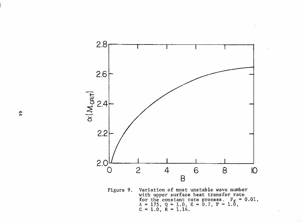
Notice now, however, that the wave number for the most critical

disturbance increases with heating rate (Figure 9) and the con-

vection cell size can be expected to decrease accordingly. B

can be varied by changing either the depth of the liquid or the

heat transfer coefficient, q, and its variation has no effect

on the solidification rate R.

A can be changed in two ways and they have different in-

fluences upon the staiblity of the system. Different materials

will have different values of L/Cps (Table II) and this will re-

sult in different values of A, for a given (TS-Tm). Keeping all

other boundary conditions constant still results in a change in

R. The effect of the change in L/C P upon Merit is shown in

32

Tabel IV and Figure 10. Materials with higher values of L/C ps

are more stable, even though the rate of solidification is also

in general faster.

A can also be varied by changing (T3-T$ but that also

changes Q. The effect of changing (Ts-Tg) in A and Q simul-

taneously, while keeping the other boundary conditions constant,

is shown in Table IV and Figure 11. Again, increasing A, through

decreasing (T$-Tz), stabilizes the flow.

As noted above, the parameters Pr, K, P, and C are con-

stant for a given material. However, the sensitivity of the

stability upon these parameters was examined so that comparison

could be made of the relative stability of different materials.

The Prandtl number can vary over many orders of magnitude,

depending upon the material (Table II). Because the Reynolds

number is directly proportional to Pr, calculations were per-

formed at constant R = 1.0 by varying A simultaneously with Pr.

The variation of the critical value of M with Pr for this case

is shown in Figures 12 and 13. Because the Maragoni number is

related to M by

M=RPr M

the variation in critical Marangoni number is very small. The

results are summarized in Table F. These results are not

accurate at the larger Pr because very large (T;-Tg) would be

required to make A small enough to keep R = 1.0.

The effect of density and specific heat ratio, P and C,

upon the critical value of M is shown in Figures 14 and 15. The

greater the increase in the density of the material upon

33

SolTdification, i.e., the lower the value of P, the more stable

the flow. Materials such as bismuth and water with values of P

greater than one are somewhat less stable than materials with

P less than one. Note that R increases somewhat as P is in-

creased verifying the previous conclusion. The same conclusion

can be drawn for increasing specific heat ratio, C (Figure 15).

C also influences R but its effect is greater than the effect of

changing R alone by changing Q.

K, the ratio of the coefficients of thermal conductivity,

can be shown to have no effect upon the stability of the system.

34

-

5.0 Conclusions

The following

of these problems:

conclusions can be drawn from the solution

1. Increasing the heat transfer rate from the upper sur-

face of the liquid by increasing the Biot.modulus, 8, stabilizes

the flow. The wave number corresponding to the most unstable

disturbance increases with B causing's corresponding decrease

in convection cell size.

2. Increasing the rate of solidification by increasing

the heat transfer rate through the solid (i.e., increasing Q

by increasing q,, ) destabilizes the flow. As Q increases the

Reynolds number, R, is increased.

3. The wave number of the most unstable disturbance is

about 2.0 to 2.2 for B = 1.0 and.varies appreciably only with

changes in B.

4. For a given temperature difference across the liquid,

"'i-T;> , materials with larger values of L/Cps are more stable

than those with smaller values.

5. Decreasing (T2 m *-T7k) while keeping other boundary con-

ditions constant stabilizes the flow.

6. The Prandtl number, Pr, has little effect upon the

critical Marangoni number for constant R.

7. Materials with larger values of density and specific

heat ratios, P and C, are less stable than those with lower

ratios.

8. The thermal conductivity ratio, K, has no effect on

the stability of the flow.

35

References

Boley, B.A. The Analysis of Problems of Heat Conduction and Melting, High Temperature Structures and Materials (Freudenthal, Boley & Liebowitt, ed.), Macmillan Co., New York, 260-315 (1964).

Busse, F.H. and Schubert, G. Convection in a Fluid with Two Phases, J, Fluid Mech., 4& 801-812 (1971).

Chang, C.E. and Wilcox, W.R. Analysis of Surface Tension Driven Flow in Floating Zone Melting, Int. J. Heat Mass Transfer, 19 355-366 (1976).

-'

Carslaw, H.S. and Jaeger, J.C. Conduction of Heat in Solids, Oxford: Clarendon Press, Chapter XI (lm).

Foust, O.J. Sodium NaK Engineering Handbook, Vol. 1, Sodium Chemistry and Physical Properties, Gordon and Breach (1972).

Levich, V.G. and Krylov, V.S. Surface Tension-Driven Phenomena, Ann. Rev. Fluid Mech., 1, 293-316 (1969).

Muehlbauer, J.C. and Sunderland, J.E. Heat Conduction with Freezing or Melting, App. Mech. Rev., 18, 951-959 (1965).

Mullins, W.W. and Sekerka, R.F. Stability of a Planar Interface during Solidification of a Dilute Binary Alloy, J. App. Physics, 35, 444-451 (1964).

Ockendon, J.R. and Hodgkins, W.R. Moving Boundary Problems in Heat Flow and Diffusion, Oxford U. Press (1975).

Pearson, J .R.A. On Convection Cells Induced by Surface Tension, J.F.M., 4, 489-550 (1958).

Rubinstein, L .I. The Stefan Problem, Trans. Math. Monographs, Vol. 27, Am. Math’. Society (1971).

Schubert, G.; Yuen, D.A.; Turcotte, D.L. Role of Phase Transition in a Dynamic Mantle, Geophys. J. R. Astr. Sot., 42, 705-735 (1975).

Seki, N .; Fukusako, S.; Sugawara, M. A Criterion of Onset of Free Convection in a Horizontal Melted Water Layer with Free Surface, J. Heat Trans., 99, 92-98 (1977).

Sparrow, E.M.; Schmidt, R.R.; and Ramsey, J.W. Experiments on the Role of Nautral Convection in the Melting of Solids, J. Heat Trans., 100, 11-16 (1978).

36

Sparrow, E.M.; Patankar, S.V.; Ramadhyoni, S. Analysis of Melting in the Presence of Natural Convection in the Melt Region, J. Heat Trans., 99 520-526 (1977). -'

Stefan, J. Ubereinige Probleme der Theorie der Wumeleitung, S.-B. Wien, Akad, Mat. Matus, 98-, 173-484 (1889).

Turcotte, D.L. Geophysical Problems with Moving Phase Change Boundaries and Heat Flow, Movin Boundar Problems in Heat Flow and Diffusion (Ockendon & HO, gklns, e . wf Clarendon Press, Oxford, 91-102 (1975).

Ukanawa, A.O. Diffusion in Liquid Metal Systems, NASA Contractor Report, Contract NAS8-30252 (1975).

West, R.C. et al. Handbook of Chemistry and Physics, 54th Edition, CRC Press (1973).

Williams, F.A. Combustion Theory, Chap. 1, Addison-Wesley (1965).

Wolkind, D.J. and Segel, L.A. A Nonlinear Stability Analysis of the Freezing of a Dilute Binary Alloy, Phil. Trans. Roy. Sot. London, 268A, 351 (1970).

37

F REE v SURFACE 4

T, -em-----,--

d -/ A-,--- ,L ,‘-,

--

Figure 1. Problem Sketch for the Steady State Solidification Process

LIQUID

z

L X

Figure 2. Sketch of the Deformation of the Liquid- Solid Interface Due to Convection in the Fluid

38

FREE v SURFACE T, d --- - - - _- ----- __

LIQUID- ----i----

Z

t X

Figure 3. Problem Sketch for the Constant Rate Solidification Process

r* s

0,2 0.4 0.0 T

Figure 4. The Non-Dimensional Temperature Profile in the Liquid for the Constant Rate Solidification Process

39

0

;, I I 0 1'00 100 200 ioo 300 3'00 400 4bo

M Figure 5. Effect of Biot modulus on the stability of the steady state

process. A = 20, y = 1.2, K = 0.7, A = 1.5.

28 .

26 .

2 3 4 B

5 6

Figure 6. Variation of most unstable wave number with upper surface heat transfer rate for the steady state pracess. A = 20, y = 1.2, A = 1.5, K = 0.7.

5-

4-

3.

o!

2

1

0 I I I I 10 20 30 40

Figure 7, Ekfect of increasing the rate of solidification on th: ;t;ktlity of the constant rate process. P, = 0.02, K = 0.5, P . , C = 1.04, A = 350, B = 1.0.

P w

5-

4--

3-

2-

l-

O-

M x lO-3 Figure 8. Effect of increasing the upper heat transfer rate on the

stability of the constant rate process. P, = 0.01, K = 0.5,

P = 0.975, c = 1.01, A = 175, Q = 1.01

2.8

26 .

20- . 0 6 8 IO

B Figure 9. Variation of most unstable wave number

with upper surface heat transfer rate for the constant rate process. Pr = 0.01, A = 175, Q = 1.0, K = 0.7, P = 1.0, C = 1.0, R = 1.14.

M GRIT

IO' L I I I I -

0 40 80 120 160 200 n

Figure 10. Effect of change in A (with constant (T2* - Tm*) upon Merit for the constant rate process. Pr = 0.01, Q = 2.0, K = 0.7, P = 1.0, C = 1.0, B = 1.0.

45

24

I6

8

4

0 0 40 80 120 160 200

Figure 11. Effect of change in (T2* - Tm*) (with qos constant) upon Merit for the constant rate problem. Pr = 0.01, K = 0.7, P = 1.0, C = 1.0, B = 1.0.

46

-

2-

l-

‘O- I I I I 0 20 40 60 610 100

Figure 12. Comparison of the stability of materials of different Prandtl numbers for the constant rate process. K = 0.7, P = 1.0, C = 1.0, Q = 1.0, R = 1.0.

0 . 2 . 4 . 6 . 8

Figure 13. Variation of Merit with Pr for R = 1.0 for the constant rate process.

i = 1.0, K = 0.7, P = 1.0, C = 1.0, = 1.0. M = R Pr M.

48

. . I mm-m.1,.

IO .

8 . 90 . 92 .94 .96 . 98

P 1.00 102 . 104 .

Figure 14. Effect of density change upon Merit for the constant rate process. P, = 0.01, A = 175, Q = 1.0, K = 0.7, B = 1.0, R = 1.1.

80 .

70 .

IO . 1.1 I2 . c

Figure 15. Effect of specific heat ratio on Merit for the constant rate process. pr = 0.02, A = 175, Q = 1.0, K = 0.5, P = 1.0, B = 1.0.

I3 .

50

TABLE I. PROPERTIES OF MATERIALS

a) Properties of Liquid State

Water 0.9998 4.218 1.79x1o-2 I

1.79x1o-2 5.66~10-~ 1.32~10-~ 0.0 I

0.0 C

b) Properties of Solid State

Bismuth 9.76 0.125 0.084 0.069 25 50.2 C

Lead 11.34 0.142 0.346 0.215 25 24.6 C

Tin 7.16 0.226 0.640 0.396 25 21.1 C

Zinc 7.40 0.389 1.150 0.400 25 102.1 C

Water 0.917 , 2.100 , 2.21x1o-2 , 1.24~10-~ , 0.0 333.5 I' c

: References: a)

b)

c>

Foust, 0. J., editor, Sodium-N,K Eng'ine'ering Handbook, Voliime '1, Sodi'um Chenii'st'ry and Physical Properties, Gordon and Breach (1972). Ukanawa, Anthony O., "Diffusion in Liquid Metal Systems," NASA Contractor Report, Contract NAS8-30252, June 1975. Handbook of Chemistry and Physics, 54th edition, CRC Press (1973).

Tdble II

VALUES OF NON-DIMENSIONAL PARAMETERS

---=..~i__ I=. i. Material

L Sodium ---~_

- I--._- --.. ..-L. __

13.6(O) 159/AT 0.255 9.41 1.090 2.008

Notes: 1. Temperatures measured in "C.

2. Properties determined at Tm*for sodium and potassium and at 25°C for the solid phase for other materials.

53

I -

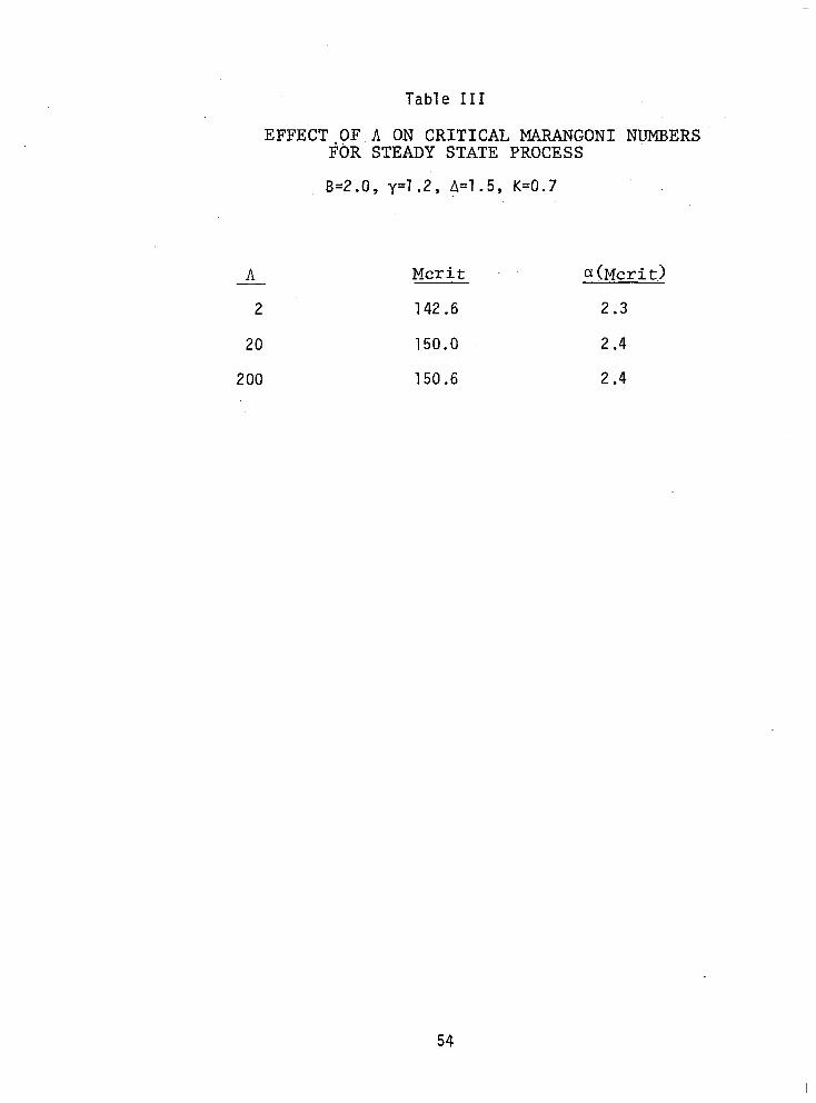
Table III

A

2

20

200

EFFECT-OF A ON CRITICAL MAWNGONI NUMBERS FOR STEADY STATE PROCESS

B=Z.O, y=1.2, A=1.5, K=0.7

Merit a(Mcrit.)

142.6 2.3

150.0 2.4

150.6 2.4

54

TABLE IV

Effect of A on Critical Marangoni Number for the Constant Rate Process

A. Effect of Change of L/CpS.

Pr=O.Ol; K=0.7; Q=Z.O; P=l.O; C=l.O; B=l.O

A

20

35

70

105

175

R

14.0

8.2

4.2

2.8

1.7

aO-fcritt>

2.1

2.1

2.1

2.1

2.2

B. Effect of Change of (9-T;).

Pr=O.Ol; K=0.7; P=l.O; C=l.O; B=l.O

A

17.5

35

70

105

175

9

0.5

1.0

2.0

3.0

5.0

R Merit aWcrit) - 8.4 6.22~10~ 2.1

5.6 1.08~10~ 2.1

4.2 1.61~10~ 2.1

3.7 1.90x103 2.1

3.1 2.18~10~ 2.1

55

I -

TABLE V

Effect of Pr on Stability for R=l.O Q=l.O; B=l.O; K=l.O; P=l .O; C=l.O

Pr

0.002

0.01

0.1

0.3

0.6

0.9

A

1000

200

20

6.0

2.7

1.5

&r-it

4.96~10~

9.96x103

1.05x103

3.59x102

2.00x102

1.45x102

Sicrit

99.2

99.6

101.8

107.7

120.0

130.5

a(Mcrit)

2.2

2.2

2.2

2.2

2.1

1.9

56

I APPENDIX I

Matching Conditions

It is necessary to determine the conditions at the liquid-solid

interface for arbitrary movement of that interface. Once the general

relations have been derived the conditions will be linearized by

assuming that the interface motion consists of a mean motion that

is one-dimensional plus a small perturbation to the mean motion.

The interface matchi,ng conditions will be written for a fixed labora-

tory frame of reference.

General interface conditions, which are expressions of the con-

servation of mass, momentum, and energy, are stated for a multi-

component system by lrlilliams (1965). These expressions can be special-

ized for a control volume consikting of a thin slab that surrounds

the interface. Assuming one-dimensional mean motion the slab control

volume in a fixed coordinate system is shown in the figure below.

A

iir 1(

': t Liquid

I I 1 .5 s(t) - Interface

J Solid

"is

57

Assume that there are no sources of mass at the surface, that the

viscous stresses can be ignored, and that no chemical reactions occur.

Write the velocities as follows: a A U = 0; u

-z -

S R = w,$ dt = vpk

A dS is the velocity of the control volume and t is a unit vector where dt

in the z direction.

The continuity equation, for this control volume [Williams, p. 141,

or

P&Vp-WJ = P, VP

The energy equation is

where

e = specific internal energy

The momentum equation becomes

Q(&)WR-vp) - p, = 0

Using this result and the continuity equation, the energy equation

can be written as

k dTs - kR dTR 'dz -

= P,(epJ & -Pi '~2 2

2 ( v -w )

dt - P R dz

But L=ell-es and the last term can be dropped because it is several

orders of magnitude smaller than the other terms. Thus, we get the

58

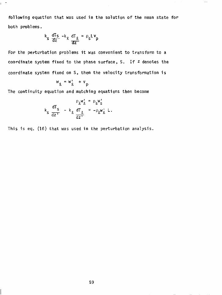
following equation that was used in the solution of the mean state for

both problems.

k dTs -kg dTR = psLv s a-z- az

P

For the perturbation problems it was convenient to transform to a

coordinate system fixed to the phase surface, S. If Z denotes the

coordinate system fixed on S, then the velocity transformation is

WR R =w’ +v P

The continuity equation and matching equations then become

kS

PRW;! dTS

dz' - kR dTR

dz'

PSWi

-Ppi L.

This is eq. (16) that was used in the perturbation analysis.

59

Appendix II

RESULTS FOR STEADY STATE PROBLEM

A B Y A K M cr.it a(M crit)

1000 0.0 0.2 1.5 0 ..7 79.603

0.5 2.0 0.2 1.5 0.7 145.7

5.0 150.2

25.0 150.6

20.0 0.0 1.2 1.5 0.7 79.0 2.0 r

I 2*o I I 150.0 I 2.4 1 I 4-o I I 216.9 I 2.5 I

I 6-O I I 282.5 I 2.6 I

2.0 2.0 1.2 1.5 0.7 142.6 2.3

200.0 2.0 1.2 1.5 0.7 150.6 2.4

60

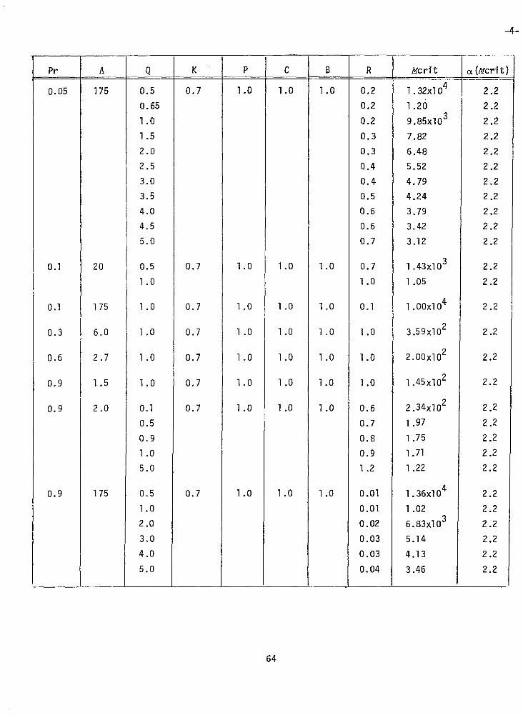
Appendix III

RESULTS FOR THE CONSTANT RATE PROCESS

Pr ___ A

0.002 17.5

0.002 175

0.002 175

..-. -.-.. -.- --.-- *R greater than 1

__- Mcrft

4.60~10~

4.19

3.47

2.81

2.38

2.07

1.85

1.67

1.53

1.42

1.33

~__--- Q K P C B R a(Mcri t) -_... _ ---.

0.50 0.7 1.0 1.0 1.0 42.0* 2.2

0.65 46.0 2.2

1.0 55.0 2.2

1.5 67.4 2.2

2.0 79.4 2.2

2.5 90.9 2.2

3.0 102.0 2.2

3.5 112.8 2.2

4.0 123.2 2.2

4.5 133.2 2.2 5.0 142.9 2.2

1.0 0.07 1.0 1 .o 1.0 5.7 2.1

1.5 7.1 2.1

2.0 8.6 2.1

2.5 10.0 2.1

3.0 11.4 2.1

3.5 12.8 2.1

4.0 14.3 2.1

4.5 15.7 2.1

5.0 17.1 2.1

0.50 0.7 1.0 1.0 1.0 4.3 2.1

0.65 4.7 2.1

1 .o 5.7 2.1

1.5 7.1 2.1

2.0 8.5 2.1

2.5 9.9 2.1 3.0 11.3 2.1

3.5 12.7 2 .l

4.0 14.1 2.1

4.5 15.4 2.1

5.0 16.8 2.2 -, -----._, - _- _-_ _ ..-- --~ 0 are in error because the linear equation was used for their determination.

61

5.22~10~

3.84

3.01

2.46

2.07

1.79

1.57

1.40

1.26

7.80~10~

6.84

5.25

3.87

3.04

2.49

2.10

1.82

1.60

1.43

1.29

___-

Pr __ .-

0.002

0.01

0.01

0.01

0.01

0.01

0.01

A

1000

17.5

20.0

35

70

105

175

175

I__- _ Q --?z-‘-r----Y

1 .o

0.50

0.50

2.0

3.0

4.0

5.0

1.0

2.0

2.0

2.0

3.0

0.60

0.65

0.70

0.90

1 .o

1.1

1.2

1.5

2.0

2.5

3.0

3.5

4.0

4.5

5.0

0.5

1.0

2.0

3.0

4.0

5.0

___-.

K .- 0.7

0.7

0.7

0.7

0.7

0.7

0.7

0.7

P

1.0

0.97

1.00

1.0

1.0

1 .o

1.0

l,.O

0.97

_-

1

-

-.-- ..- - C

1 .o

1.0

1.0

1.0

1 .o

1.0

1.0

1 .o

.-_-

B

1.0

1.0

1.0

1.0

1.0

1 .o

1.0

1 .o

R

1.0

Mcri t

4.96~10~

a(Mcrit)

2.2

8.2 6.50~10~ 2.1

8.4 6.28~10~ 2.1

14.0 3.29x102 2.1

18.1 2.44 2.15

21.9 1.96 2.2

25.5 1.66 2.2

5.6 1.08~10~

8.2 6.4~10~

4.2 1.61~10~

2.8 2.76~10~

3.7 1 .90

0.9 1.10x104

0.9 1.06

1.0 1.03

1.1 9.05x103

1.1 8.53

1.2 8.06

1.2 7.64

1.4 6.57

1.7 5.27

2.0 4.36

2.3 3.69

2.5 3.17

2.8 2.77

3.1 2.45

3.4 2.18

2.1

2.1

2.1

2.1

2.1

2.2

2.2

2.2

2.2

2.2

2.2

2.2

2.2

2.2

2.1

2.1

2.1 (

2.1 1

2.1 j

2.1 j

0.8

1.1

1.6

2.2

2.7

3.3 _-- --

1.23~10~

8.89x103

5.51

3.87

2.91

2.30

2.2 1

2.2 /

2.2 /

2.1 1

2.1 1

2.1 I

-

-2-

62

0.01

0.01

0.01

0.02

0.02

A

175

175

175

200

175

350

-

- .i _. Q

1.0

1 .o

1.0

1.0

1 .o

0.5

1.0

2.0

3.0

4.0

5.0

K .r: .ET ._

0.7

0.7

0.5

0.7

0.5

0.5

P ..- -.- 0.90

0.92

0.94

0.96

0.98

1.02

1.04

1.0

0.975

1.0

1.0

0.965

C

1.0

1.0

1 .Ol

1.0

1.0

1.01

1.04

1.10

1.30

1.04

- -

B

1 .o

0.1

0.3

0.7

1.0

3.0

7.0

10.0

0.1

0.3

1.0

3.0

10.0

1.0

1 .o

1.0

R __--.--.

1.0

1.0

1 .l

1.1

1.1

1.2

1.2

Merit a(Mcri t)

9.79x103 2.2

9.52 2.2

9.26 2.2

9.01 2.2

8.77 2.2

8.31 2.2

8.10 2.2

1.1 6.09x103 2.0

6.65 2.0

7.74 2.1

8.53 2.2

1 .37x104 2.4

2.35 2.6

3.09 2.65

1.1 6.22~10~ 2.0

6.79 2.0

8.71 2.2

1.39x104 2.4

3.15 2.7

1.0 9.96x103

0.6 9.30x103

0.6 9.20

0.6 8.92

0.6 8.39

0.7 6.97

0.2

0.3

0.4

0.6

0.7

0.8 - _.

2.61~10~

1.94

1.27

9.31x103

7.31

5.97

2.2

2.2

2.2

2.2

2.2

2.2

2.2

2.2

2.2

2.2

2.2

2.2

63

Pr

0.05

0.1

0.1

0.3

0.6

0.9

0.9

0.9

A

175

20

175

6.0

2.7

1.5

2.0

175

Q

0.5

0.65

1.0

1.5

2.0

2.5

3.0

3.5

4.0

4.5

5.0

0.5

1.0

1.0

1.0

1.0

1.0

0.1

0.5

0.9

1 .o

5.0

0.5

1.0

2.0

3.0

4.0

5.0

K

0.7

0.7

0.7

0.7

0.7

0.7

0.7

0.7

P

1 .o

1.0

1.0

1.0

1.0

1.0

1 .o

1.0

C

1.0

1 .o

1.0

1.0

1.0

1.0

1 .o

1.0

B

1.0

1.0

1.0

1 .o

1.0

1 .o

1 .o

1.0

___-

R

0.2

0.2

0.2

0.3

0.3

0.4

0.4

0.5

0.6

0.6

0.7

Mcri t ---.----rz 1.32~10~

1.26

9.85x103

7.82

6.48

5.52

4.79

4.24

3.79

3.42

3.12

0.7

1.0

1.43x103

1.05

0.1 1.00x104

1.0 3.59x102

1.0 2.00x102

1 .o 1.45x102

0.6

0.7

0.8

0.9

1.2

2.34x102

1.97

1.75

1.71

1.22

0.01 1.36~10~

0.01 1.02

0.02 6.83~10~

0.03 5.14

0.03 4.13

0.04 3.46

-. _ ._..~

a(Mcri

2.2

2.2

2.2

2.2

2.2

2.2

2.2

2.2

2.2

2.2

2.2

2.2

2.2

2.2

2.2

2.2

2.2

2.2

2.2

2.2

2.2

2.2

2.2

2.2

2.2

2.2

2.2

2.2

-4-

J t) _--I

64

Pr

10

10

A .^ _ _ - . -. 2.0

175

Q ” .:-1- 0.5

1.0

2.0

3.0

4.0

5.0

0.5

1.0

2.0

3.0

4.0

5.0

-

^ _ _ - - K

_ .- - 0.7

0.7

.._... P

_-__ 1.0

1.0

C

1.0

1 .o

B

1.0

1.0

0.06

0.07

0.09

0.10

0.10

0.11

. .._ . -- .___.., Merit

2.19x102

1 .94

1 .69

1.58

1 .51

1.46

1.36~10~

1.02

6.85~10~

5.16

4.15

3.48

a(Mcrit)

2.2

2.2

2.2

2.2

2.2

2.2

2.2

65

TECHNICAL REPORT STANDARD TITLE PAGI

1. REPORT NO. 12. GOVEf?NhlENT ACCESSION NO. 3. RECIPIENT’S CATALOG NO.

NASA CR-3051 I 4. TITLE AND SUBTITLE 5. REPORT DATE

September 1978 Studies of Convection in a Solidifying System with Surface 6. PERFORMING ORGANIZATION CODE

Tension at Reduced Gravity I 7. AUTHOR(S) 3. PERFORMING ORGANIZATION REPOR r I

Basil N. Antar and Frank G,. Collins 9. PERFORMING ORGANIZATION NAME AND ADDRESS 10. WORK UNIT, NO.

M-265 The University of Tennessee Space Institute 1 ,. CONTRACT OR GRANT NO.

Tullahoma, Tennessee NAS&32484. 13. TYPE OF REPOR;’ & PERIOD COVEREl

12. SPONSORING AGENCY NAME AND ADDRESS

Contractor

National Aeronautics and Space Administration Washington, D. C. 20546

1.1, SPONSORING AGENCY CODE

15. SUPPLEMENTARY NOTES

Prepared under the technical monitorship of the Aerospace Sciences Division, Space Sciences Laboratory, NASA/Marshall Space Flight Center

lb. ABSTRACT

The “low gravity” environment of Earth’s orbit is being seriously considered for experimentation on the production of materials in space. Most of such materials processes inevitably involve either the solidification of melt or the melting of solids. Inherent in most fluid mechanisms with temperature gradients is convective motion. In this report a study is presented for the onset of convection in a solidifying system in an environment which is similar to that encountered in space processing. Since the study is for a “low gravity” condition, the only driving mechanism considered is that due to the variation of surface tension force at the free surface of the melt layer. Two simple solidification models are considered, one in which the solidification process enters in the perturbation system and another in which the melt is solidifying at a constant rate. The results show that the solidification process will bring about convection in the melt earlier than otherwise.

7. KEY WORDS 18. DISTRIBUTION STATEMENT

Category 34

,3. SECURITY CLASSIF. (of tbla report)

Unclassified

I

20. SECURITY CLASSIF. (of this ww) 21. NO. OF PAGES 22. PRICE

Unclassified 69 $5.25 VGFC - Form 5292 (hcl

‘For sale by the National Technical Information Service, Springfield. Virginia 22161

NASA-Langley, 1978