STUDIES OF GROUNDWATER EXPLORATION IN … · conductivity are Siemens per meter ... well connected by Mysore to Chamarajanagar broad gauge ... current electrodes and the potential

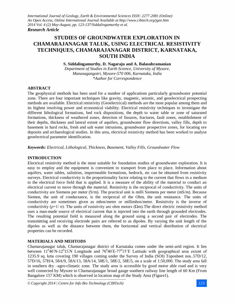
International Journal of Geology, Earth & Environmental Sciences ISSN: 2277-2081 (Online)

An Open Access, Online International Journal Available at http://www.cibtech.org/jgee.htm

2014 Vol. 4 (2) May-August, pp. 123-137/Siddalingamurthy et al.

Research Article

© Copyright 2014 | Centre for Info Bio Technology (CIBTech) 123

STUDIES OF GROUNDWATER EXPLORATION IN

CHAMARAJANAGAR TALUK, USING ELECTRICAL RESISTIVITY

TECHNIQUES, CHAMARAJANAGAR DISTRICT, KARNATAKA,

SOUTH INDIA

S. Siddalingamurthy, D. Nagaraju and A. Balasubramanian Department of Studies in Earth Science, University of Mysore,

Manasagangotri, Mysore-570 006, Karnataka, India

*Author for Correspondence

ABSTRACT

The geophysical methods has been used for a number of applications particularly groundwater potential

zone. There are four important techniques like gravity, magnetic, seismic, and geoelectrical prospecting methods are available. Electrical resistivity (Geoelectrical) methods are the most popular among them and

its highest resolving power and economical viability. Electrical resistivity techniques to investigate the

different lithological formations, bed rock dispositions, the depth to water table or zone of saturated formations, thickness of weathered zones, detection of fissures, fractures, fault zones, establishment of

their depths, thickness and lateral extent of aquifers, groundwater flow directions, valley fills, depth to

basement in hard rocks, fresh and salt water intrusions, groundwater prospective zones, for locating ore

deposits and archaeological studies. In this area, electrical resistivity method has been worked to analyse geoelectrical parameter identification.

Keywords: Electrical, Lithological, Thickness, Basement, Valley Fills, Groundwater Flow

INTRODUCTION

Electrical resistivity method is the most suitable for foundation studies of groundwater exploration. It is easy to employ and the equipment is convenient to transport from place to place. Information about

aquifers, water tables, salinities, impermeable formations, bedrock, etc can be obtained from resistivity

surveys. Electrical conductivity is the proportionality factor relating to the current that flows in a medium to the electrical force field that is applied. It is a measure of the ability of the material to conduct an

electrical current to move through the material. Resistivity is the reciprocal of conductivity. The units of

conductivity are Siemens per meter (S/m). The practical unit is milli Siemens per meter (mS/m). Because

Siemen, the unit of conductance, is the reciprocal of the Ohm, the unit resistance. The units of conductivity are sometimes given as mhos/meter or millimhos/meter. Resistivity is the inverse of

conductivity (ρ=1/ σ). The units of resistivity are ohm meters (Ώm).The direct electric resistivity method

uses a man-made source of electrical current that is injected into the earth through grounded electrodes. The resulting potential field is measured along the ground using a second pair of electrodes. The

transmitting and receiving electrode pairs are referred to as dipoles. By varying the unit length of the

dipoles as well as the distance between them, the horizontal and vertical distribution of electrical properties can be recorded.

MATERIALS AND MEHTODS

Chamarajanagar taluk, Chamarajanagar district of Karnataka comes under the semi-arid region. It lies

between 11040

’N-12

015

’N Longitude and 76

040

’E-77

015’E Latitude with geographical area extent of

1235.9 sq. kms covering 190 villages coming under the Survey of India (SOI) Toposheet nos..57D/12,

57D/16, 57H/4, 58A/9, 58A/13, 58A/14, 58E/1, 58E/2, 58E/5, on a scale of 1:50,000. The study area fall

in southern dry –agro-climatic zone. The study area is accessible by good motor able road and is very

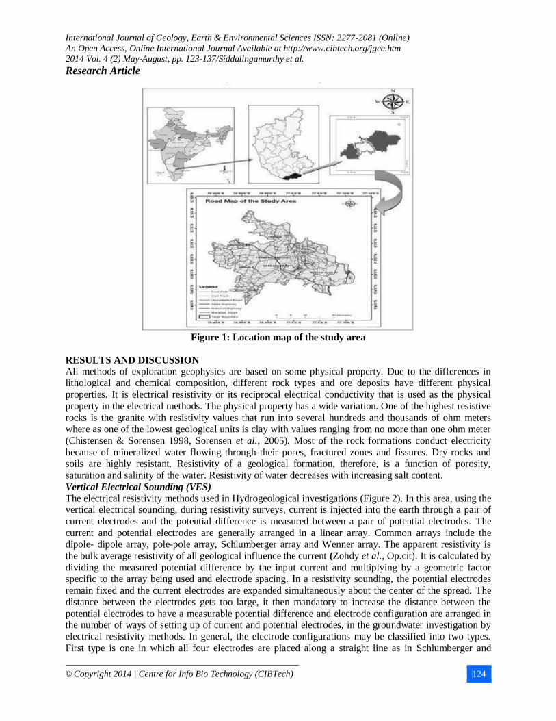
well connected by Mysore to Chamarajanagar broad gauge southern railway line length of 60 Km (From Bangalore 157 KM) which is observed in location map of the Study Area (Figure1).




Research Article


Figure 1: Location map of the study area

RESULTS AND DISCUSSION

All methods of exploration geophysics are based on some physical property. Due to the differences in lithological and chemical composition, different rock types and ore deposits have different physical

properties. It is electrical resistivity or its reciprocal electrical conductivity that is used as the physical

property in the electrical methods. The physical property has a wide variation. One of the highest resistive

rocks is the granite with resistivity values that run into several hundreds and thousands of ohm meters where as one of the lowest geological units is clay with values ranging from no more than one ohm meter

(Chistensen & Sorensen 1998, Sorensen et al., 2005). Most of the rock formations conduct electricity

because of mineralized water flowing through their pores, fractured zones and fissures. Dry rocks and soils are highly resistant. Resistivity of a geological formation, therefore, is a function of porosity,

saturation and salinity of the water. Resistivity of water decreases with increasing salt content.

Vertical Electrical Sounding (VES)

The electrical resistivity methods used in Hydrogeological investigations (Figure 2). In this area, using the vertical electrical sounding, during resistivity surveys, current is injected into the earth through a pair of

current electrodes and the potential difference is measured between a pair of potential electrodes. The

current and potential electrodes are generally arranged in a linear array. Common arrays include the dipole- dipole array, pole-pole array, Schlumberger array and Wenner array. The apparent resistivity is

the bulk average resistivity of all geological influence the current (Zohdy et al., Op.cit). It is calculated by

dividing the measured potential difference by the input current and multiplying by a geometric factor specific to the array being used and electrode spacing. In a resistivity sounding, the potential electrodes

remain fixed and the current electrodes are expanded simultaneously about the center of the spread. The

distance between the electrodes gets too large, it then mandatory to increase the distance between the

potential electrodes to have a measurable potential difference and electrode configuration are arranged in the number of ways of setting up of current and potential electrodes, in the groundwater investigation by

electrical resistivity methods. In general, the electrode configurations may be classified into two types.

First type is one in which all four electrodes are placed along a straight line as in Schlumberger and




Research Article


Wenner array. Second type is one in which the pairs of current and potential electrodes are separately

placed and they are not supposed to be in a straight line as in dipole-dipole array. The first type is being

widely employed for groundwater studies the variation of resistivity with depth is modeled using forward and inverse modeling computer software IPI2WIN.

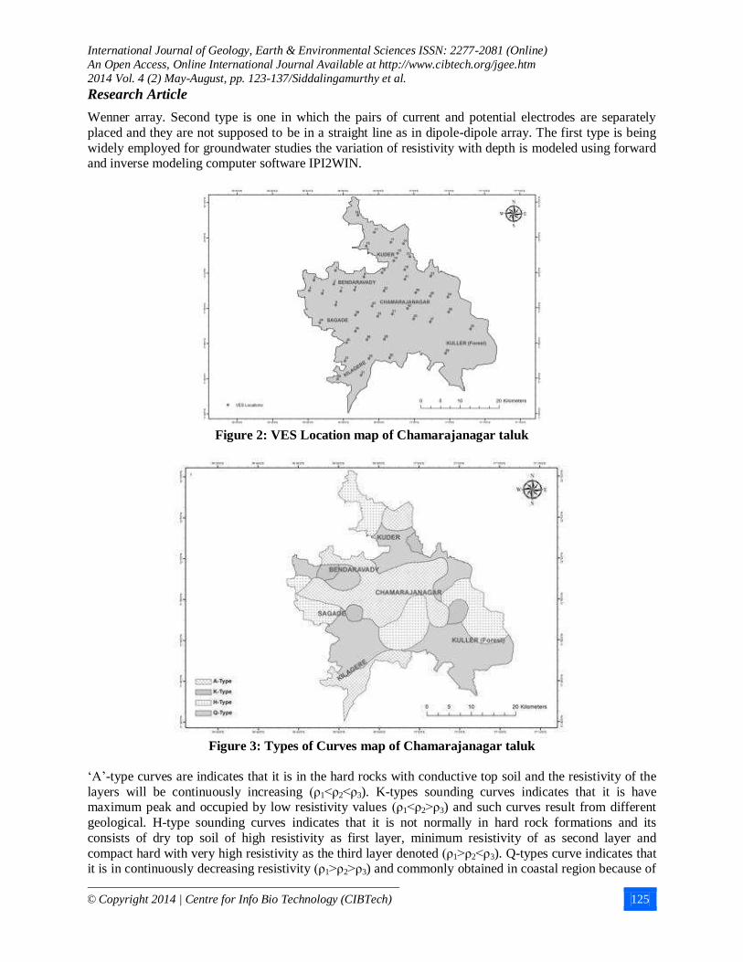
Figure 2: VES Location map of Chamarajanagar taluk

Figure 3: Types of Curves map of Chamarajanagar taluk

‘A’-type curves are indicates that it is in the hard rocks with conductive top soil and the resistivity of the

layers will be continuously increasing (ρ1<ρ2<ρ3). K-types sounding curves indicates that it is have maximum peak and occupied by low resistivity values (ρ1<ρ2>ρ3) and such curves result from different

geological. H-type sounding curves indicates that it is not normally in hard rock formations and its

consists of dry top soil of high resistivity as first layer, minimum resistivity of as second layer and

compact hard with very high resistivity as the third layer denoted (ρ1>ρ2<ρ3). Q-types curve indicates that it is in continuously decreasing resistivity (ρ1>ρ2>ρ3) and commonly obtained in coastal region because of




Research Article


the saline water. Based on the above results interpretation of the Chamarajanagar taluk, the following

types of curves are noticed (Figure 3).

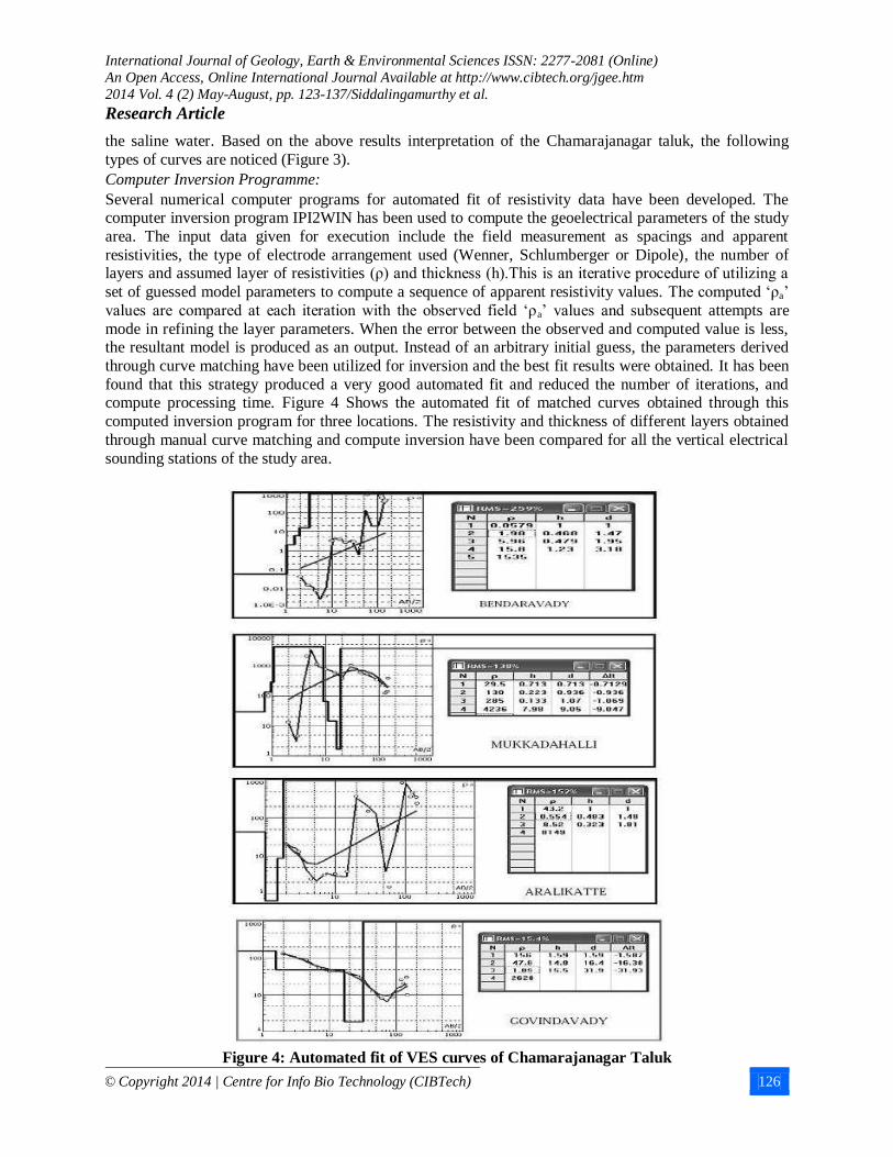
Computer Inversion Programme:

Several numerical computer programs for automated fit of resistivity data have been developed. The computer inversion program IPI2WIN has been used to compute the geoelectrical parameters of the study

area. The input data given for execution include the field measurement as spacings and apparent

resistivities, the type of electrode arrangement used (Wenner, Schlumberger or Dipole), the number of layers and assumed layer of resistivities (ρ) and thickness (h).This is an iterative procedure of utilizing a

set of guessed model parameters to compute a sequence of apparent resistivity values. The computed ‘ρa’

values are compared at each iteration with the observed field ‘ρa’ values and subsequent attempts are

mode in refining the layer parameters. When the error between the observed and computed value is less, the resultant model is produced as an output. Instead of an arbitrary initial guess, the parameters derived

through curve matching have been utilized for inversion and the best fit results were obtained. It has been

found that this strategy produced a very good automated fit and reduced the number of iterations, and compute processing time. Figure 4 Shows the automated fit of matched curves obtained through this

computed inversion program for three locations. The resistivity and thickness of different layers obtained

through manual curve matching and compute inversion have been compared for all the vertical electrical

sounding stations of the study area.

Figure 4: Automated fit of VES curves of Chamarajanagar Taluk




Research Article


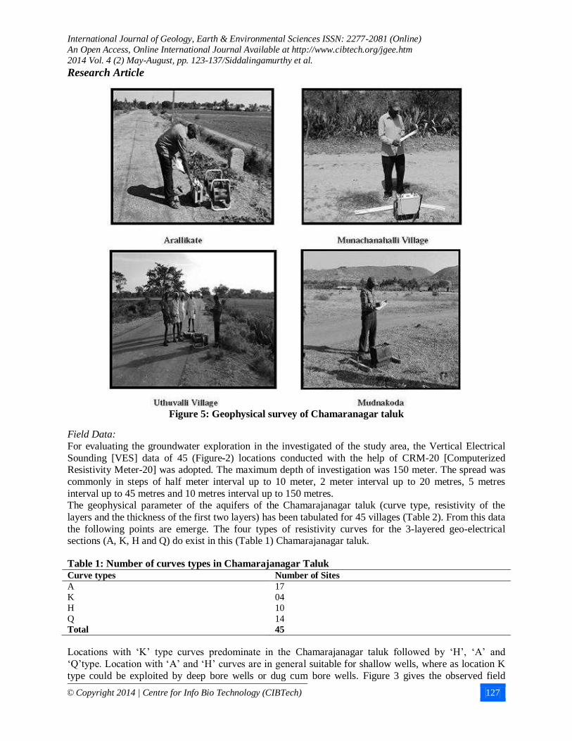
Figure 5: Geophysical survey of Chamaranagar taluk

Field Data:

For evaluating the groundwater exploration in the investigated of the study area, the Vertical Electrical

Sounding [VES] data of 45 (Figure-2) locations conducted with the help of CRM-20 [Computerized Resistivity Meter-20] was adopted. The maximum depth of investigation was 150 meter. The spread was

commonly in steps of half meter interval up to 10 meter, 2 meter interval up to 20 metres, 5 metres

interval up to 45 metres and 10 metres interval up to 150 metres. The geophysical parameter of the aquifers of the Chamarajanagar taluk (curve type, resistivity of the

layers and the thickness of the first two layers) has been tabulated for 45 villages (Table 2). From this data

the following points are emerge. The four types of resistivity curves for the 3-layered geo-electrical sections (A, K, H and Q) do exist in this (Table 1) Chamarajanagar taluk.

Table 1: Number of curves types in Chamarajanagar Taluk Curve types Number of Sites

A 17

K 04

H 10

Q 14

Total 45

Locations with ‘K’ type curves predominate in the Chamarajanagar taluk followed by ‘H’, ‘A’ and

‘Q’type. Location with ‘A’ and ‘H’ curves are in general suitable for shallow wells, where as location K

type could be exploited by deep bore wells or dug cum bore wells. Figure 3 gives the observed field




Research Article


curves as well as computed field model curves using the IPI2WIN program along with the geoelectrical

model. These diagrams show clearly that the IPI2WIN model exactly coincides with the field data and

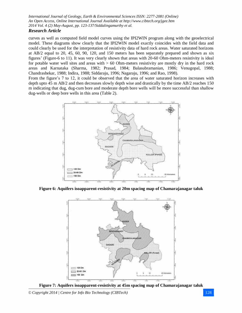
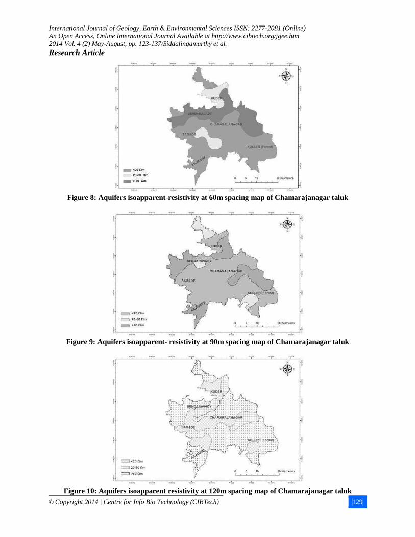
could clearly be used for the interpretation of resistivity data of hard rock areas. Water saturated horizons at AB/2 equal to 20, 45, 60, 90, 120, and 150 meters has been separately prepared and shown as six

figures’ (Figure-6 to 11). It was very clearly shown that areas with 20-60 Ohm-meters resistivity is ideal

for potable water well sites and areas with > 60 Ohm-meters resistivity are mostly dry in the hard rock areas and Karnataka (Sharma, 1982; Prasad, 1984; Balasubramanian, 1986; Venugopal, 1988;

Chandrashekar, 1988; Indira, 1988; Siddaraju, 1996; Nagaraju, 1996; and Rao, 1998).

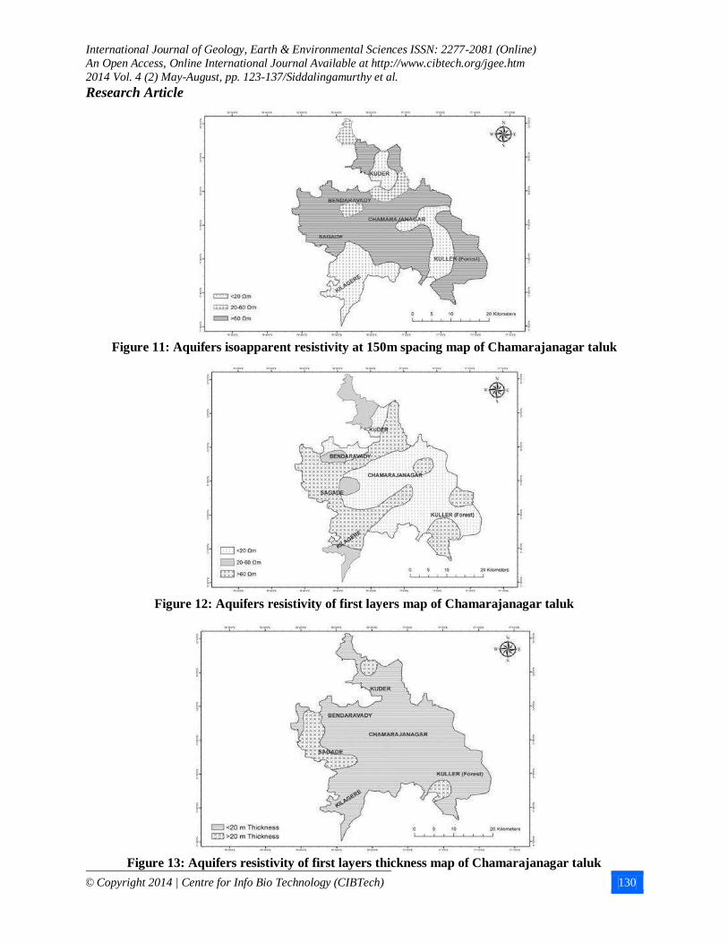
From the figure’s 7 to 12, it could be observed that the area of water saturated horizon increases with

depth upto 45 m AB/2 and then decreases slowly depth wise and drastically by the time AB/2 reaches 150 m indicating that dug, dug-cum bore and moderate depth bore wells will be more successful than shallow

dug-wells or deep bore wells in this area (Table 2).

Figure 6: Aquifers isoapparent-resistivity at 20m spacing map of Chamarajanagar taluk





Research Article



Figure 9: Aquifers isoapparent- resistivity at 90m spacing map of Chamarajanagar taluk

Figure 10: Aquifers isoapparent resistivity at 120m spacing map of Chamarajanagar taluk




Research Article


Figure 11: Aquifers isoapparent resistivity at 150m spacing map of Chamarajanagar taluk

Figure 12: Aquifers resistivity of first layers map of Chamarajanagar taluk

Figure 13: Aquifers resistivity of first layers thickness map of Chamarajanagar taluk




Research Article


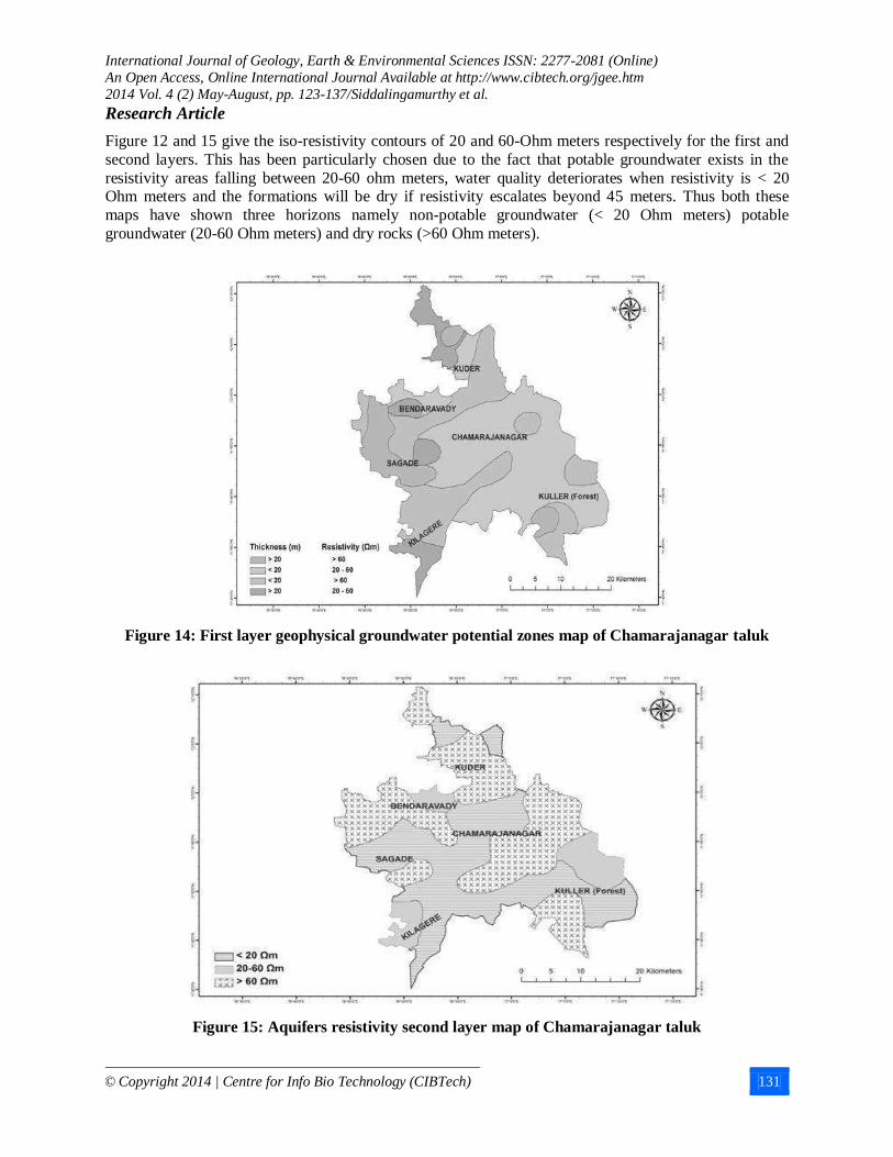
Figure 12 and 15 give the iso-resistivity contours of 20 and 60-Ohm meters respectively for the first and

second layers. This has been particularly chosen due to the fact that potable groundwater exists in the

resistivity areas falling between 20-60 ohm meters, water quality deteriorates when resistivity is < 20 Ohm meters and the formations will be dry if resistivity escalates beyond 45 meters. Thus both these

maps have shown three horizons namely non-potable groundwater (< 20 Ohm meters) potable

groundwater (20-60 Ohm meters) and dry rocks (>60 Ohm meters).

Figure 14: First layer geophysical groundwater potential zones map of Chamarajanagar taluk

Figure 15: Aquifers resistivity second layer map of Chamarajanagar taluk




Research Article


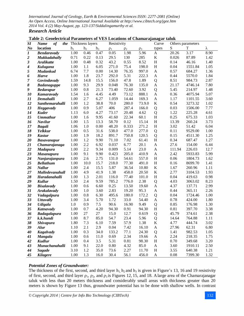
Table 2: Geoelectrical Parameters of VES Locations of Chamarajanagar taluk SI

No

Name of the

location

Thickness layers Resistivity Curve

types

Others parameters

h1 h2 h3 ρ1 ρ2 ρ3 S T λ

1 Bendaravady 1.00 0.46 0.47 0.05 1.98 5.96 A 20.26 3.17 8.90

2 Mukkadahally 0.71 0.22 0.13 29.5 130 285 K 0.026 87.89 1.42

3 Aralikatte 1.00 0.48 0.32 43.2 0.55 8.52 H 0.14 46.16 1.40

4 Kulugana 1.00 1.1 6.05 271.0 75.4 198.0 H 0.04 1551.84 1.05

5 Mudankud 6.74 7.7 0.00 14.30 76.35 997.0 A 0.57 684.27 1.36

6 Harve 1.00 1.8 23.7 292.0 5.31 222.3 A 0.44 5570.0 1.84

7 Govindavady 1.59 14.8 15.5 156.0 47.8 1.89 Q 8.51 984.73 2.87

8 Badanaguppe 1.00 9.3 29.9 0.048 76.30 135.0 A 21.17 4746.14 7.80

9 Bedarapur 1.00 0.8 21.3 73.40 72.60 3.92 Q 5.45 214.97 1.48

10 Kamaravady 1.54 1.6 4.45 4.49 73.12 888.1 A 0.36 4075.94 5.07

11 Demahalli 1.00 2.7 6.27 1.059 14.44 169.3 A 1.17 1101.55 3.60

12 Santhemarahalli 1.00 1.2 38.8 70.0 280.0 73.9.0 K 0.54 3273.32 1.02

13 Heggavady 1.00 0.9 5.07 406 287.4 166.0 Q 0.03 1506.00 7.77

14 Kuder 1.13 6.0 4.27 73.17 20.48 4.62 Q 1.22 225.28 4.61

15 Ummathur 1.00 1.6 9.95 41.60 22.34 60.1 H 0.25 675.33 1.03

16 Navilur 1.00 1.5 13.3 58.70 0.12 15.14 H 13.39 260.24 3.73

17 Bagali 1.06 1.0 0.00 48.20 0.333 271.2 H 3.02 51.42 6.04

18 Yelkkur 1.00 0.5 31.6 538.0 477.0 277.0 Q 0.11 9529.00 1.00

19 Kastur 1.00 1.9 18.2 891.7 750.8 120.5 Q 0.15 4511.30 1.25

20 Basavanapur 1.00 1.2 9.90 71.10 7.02 61.41 H 0.34 687.47 1.27

21 Chamarajanaga 1.00 2.2 6.92 0.037 6.77 20.1 A 27.6 154.00 6.44

22 Madapura 1.00 2.2 9.34 0.009 5.14 23.0 A 111.94 226.03 12.7

23 Masanapura 1.00 9.1 9.90 0.423 205.0 410.9 A 2.42 5933.83 5.99

24 Nanjarajanpura 1.00 2.6 2.75 131.0 54.61 557.0 H 0.06 1804.73 1.62

25 Bellathum 1.00 10.0 15.7 218.0 77.30 491.0 H 0.16 8699.70 1.41

26 Nallur 1.00 2.4 15.5 5.87 36.54 10.80 K 1.67 260.96 1.11

27 Malledevanahall 1.00 4.9 41.9 1.38 458.0 20.50 K 2.77 3104.53 1.93

28 Haradanahalli 1.00 1.3 2.01 116.0 77.40 101.0 H 0.04 419.63 0.98

29 Kullur 1.50 2.4 9.59 785.2 776.0 2.38 Q 4.03 3063.02 8.23

30 Bisalavady 1.00 0.6 6.60 0.25 13.50 19.60 A 4.37 137.71 2.99

31 Arakalavady 1.00 1.0 3.60 2.83 19.20 95.3 A 0.44 365.11 2.26

32 Vadagalpura 1.00 0.8 6.30 495.6 180.0 172.2 Q 0.04 1724.46 1.00

33 Uttuvally 1.00 3.4 5.70 1.72 33.0 54.40 A 0.78 424.00 1.80

34 Udigala 1.0 0.9 7.5 90.6 16.90 9.49 Q 0.85 176.98 1.30

35 Katnavady 1.00 0.7 4.20 94.30 0.91 94.30 H 0.81 397.70 3.38

36 Badagalapura 1.00 27 27 15.0 12.7 0.619 Q 45.79 374.61 2.38

37 k.k.hundi 1.00 8.7 85.0 54.7 23.4 5.96 Q 14.64 764.88 1.11

38 Shivapura 1.80 7.3 6.10 7.59 57.9 1.38 K 4.77 444.74 3.02

39 Alur 1.10 2.1 2.9 0.04 7.42 16.10 A 27.96 62.31 6.80

40 Kagalvady 1.00 0.3 34.0 133.2 77.1 24.30 Q 1.41 982.53 1.05

41 Mangala 1.00 0.6 11.0 0.69 2.34 19.66 A 2.24 218.35 1.75

42 Kudlur 1.00 0.4 3.5 5.31 0.81 98.30 H 0.70 349.68 3.20

43 Munachanahalli 1.00 9.1 22.0 0.80 4.32 85.0 A 3.60 1910.11 2.50

44 Sagade 3.10 1.2 35.0 73.6 2.27 11.70 H 3.55 640.38 1.21

45 Kilagere 1.00 1.3 16.0 30.4 56.1 456.0 A 0.08 7399.30 1.32

Potential Zones of Groundwater: The thickness of the first, second, and third layer h1, h2 and h3 is given in Figure’s 13, 16 and 19 resistivity

of first, second, and third layer ρ1, ρ2, and ρ3 is Figures 12, 15, and 18. A large area of the Chamarajanagar

taluk with less than 20 meters thickness and considerably small areas with thickness greater than 20 meters is shown by Figure 13 thus, groundwater potential has to be done with shallow wells. In contrast




Research Article


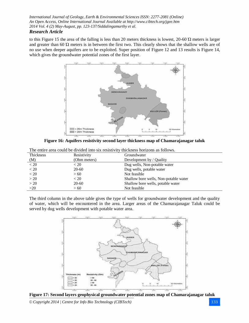
to this Figure 15 the area of the falling is less than 20 meters thickness is lowest, 20-60 Ώ meters is larger

and greater than 60 Ώ meters is in between the first two. This clearly shows that the shallow wells are of

no use when deeper aquifers are to be exploited. Super position of Figure 12 and 13 results is Figure 14, which gives the groundwater potential zones of the first layer.

Figure 16: Aquifers resistivity second layer thickness map of Chamarajanagar taluk

The entire area could be divided into six resistivity thickness horizons as follows. Thickness

(M)

Resistivity

(Ohm meters)

Groundwater

Development by / Quality

< 20

< 20

< 20

> 20

> 20

>20

< 20

20-60

> 60

< 20

20-60

> 60

Dug wells, Non-potable water

Dug wells, potable water

Not feasible

Shallow bore wells, Non-potable water

Shallow bore wells, potable water

Not feasible

The third column in the above table gives the type of wells for groundwater development and the quality of water, which will be encountered in the area. Larger areas of the Chamarajanagar Taluk could be

served by dug wells development with potable water area.

Figure 17: Second layers geophysical groundwater potential zones map of Chamarajanagar taluk




Research Article


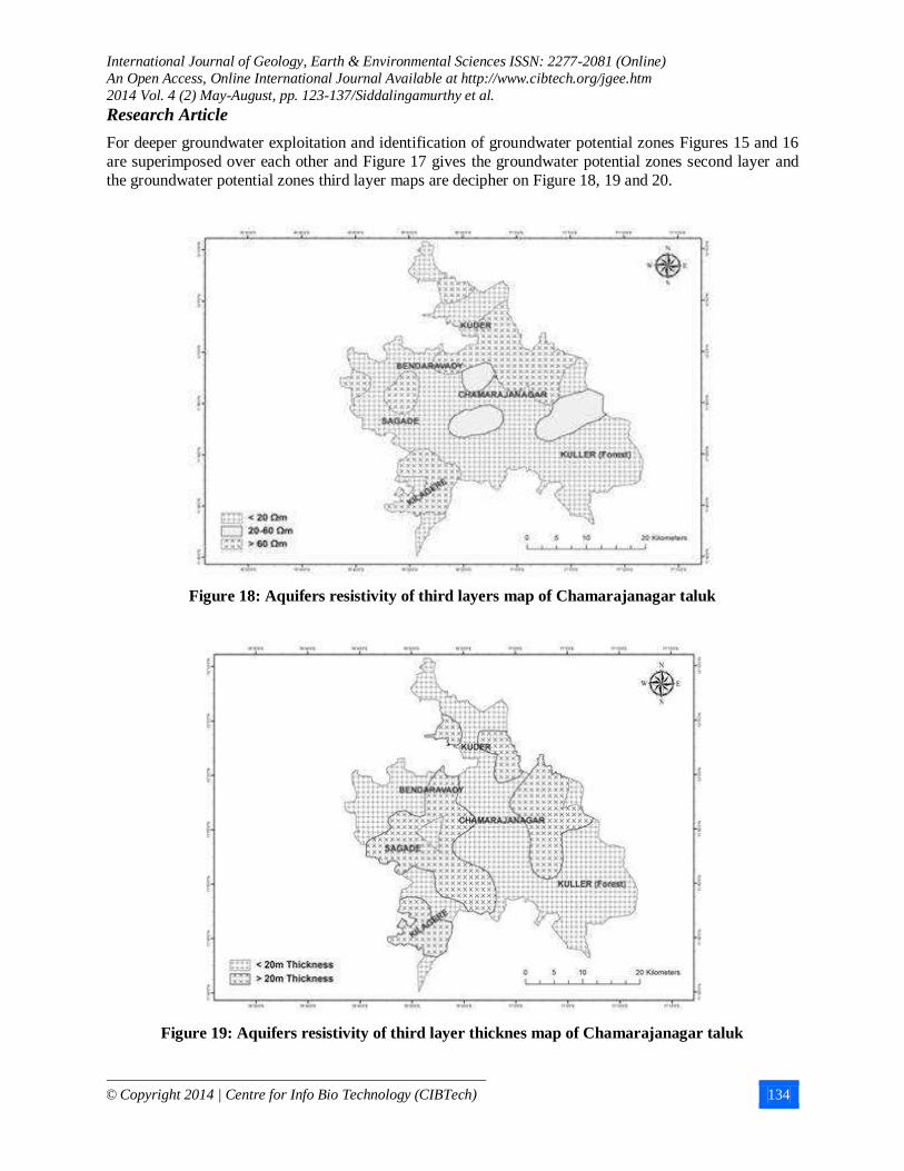
For deeper groundwater exploitation and identification of groundwater potential zones Figures 15 and 16

are superimposed over each other and Figure 17 gives the groundwater potential zones second layer and

the groundwater potential zones third layer maps are decipher on Figure 18, 19 and 20.

Figure 18: Aquifers resistivity of third layers map of Chamarajanagar taluk

Figure 19: Aquifers resistivity of third layer thicknes map of Chamarajanagar taluk




Research Article


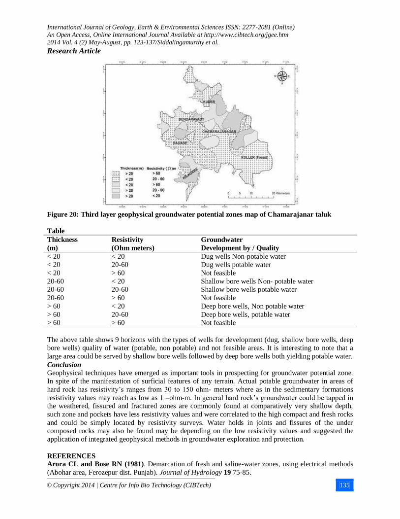
Figure 20: Third layer geophysical groundwater potential zones map of Chamarajanar taluk

Table

Thickness

(m)

Resistivity

(Ohm meters)

Groundwater

Development by / Quality

< 20 < 20

< 20

20-60 20-60

20-60

> 60

> 60 > 60

< 20 20-60

> 60

< 20 20-60

> 60

< 20

20-60 > 60

Dug wells Non-potable water Dug wells potable water

Not feasible

Shallow bore wells Non- potable water Shallow bore wells potable water

Not feasible

Deep bore wells, Non potable water

Deep bore wells, potable water Not feasible

The above table shows 9 horizons with the types of wells for development (dug, shallow bore wells, deep bore wells) quality of water (potable, non potable) and not feasible areas. It is interesting to note that a

large area could be served by shallow bore wells followed by deep bore wells both yielding potable water.

Conclusion

Geophysical techniques have emerged as important tools in prospecting for groundwater potential zone. In spite of the manifestation of surficial features of any terrain. Actual potable groundwater in areas of

hard rock has resistivity’s ranges from 30 to 150 ohm- meters where as in the sedimentary formations

resistivity values may reach as low as 1 –ohm-m. In general hard rock’s groundwater could be tapped in the weathered, fissured and fractured zones are commonly found at comparatively very shallow depth,

such zone and pockets have less resistivity values and were correlated to the high compact and fresh rocks

and could be simply located by resistivity surveys. Water holds in joints and fissures of the under composed rocks may also be found may be depending on the low resistivity values and suggested the

application of integrated geophysical methods in groundwater exploration and protection.

REFERENCES Arora CL and Bose RN (1981). Demarcation of fresh and saline-water zones, using electrical methods

(Abohar area, Ferozepur dist. Punjab). Journal of Hydrology 19 75-85.




Research Article


Balasubramanian A (1986). Hydrogeological investigations in the Tambraparni River Basin, Tamilnadu.

Unpublished Ph.D. thesis, University of Mysore 349.

Bhattacharya PK and Patra HP (1968). Direct Current Geoelectric Sounding: Principle and Interpretation (Elsevier Pub. Co.: Amsterdam, Netherlands) 135.

Bhima Shnakaram VLS and Gour VK., Pub., AEG, Hyderabad pp. 375-404.

Bhimashankaram VLS and Gaur KV (1977). Lectures on Exploration Geophysics for Geologists and Engineers (AEG Publ., Osmania Uni. Hyderabad) 449.

Christensen NB and Sorensen KI (1998). Surface and borehole electric and electromagnetic methods

for hydrogeological investigations. European Journal of Environmental and Engineering Geophysics 3

75–90. Compagnie generalae de Geophysique, CGG (1963). Master curves for eledrical sounding (2nd revised

edition): L&den, Eur. Assoc. of Explr. Geophys. Dakhnov, V. N., 1953, Electrical prospecting for

petroleum and natural gas deposits: Moscow, Gostoptekhizdat, 497 p Flathe (1963). Five-layer master curvets for the hydrogeological interpretation of geoelectric resistivity

measurements above a two story aquifer. Geophysical Prospecting 11 471-508.

Galin DL (1979). Use longitudinal conductance in vertical electrical sounding induced potential method for solving hydrogeological problems, vestrick moskovs kogo universiteta. Geologiya 34(3) 97-100.

Gilkeson RH and Cartwright (1983). The application of surface electrical and shallow Geothermic

methods in monitoring network design: Ground Water Monitoring Review 3(3) 30-42.

Henriet JP (1975). Direct interpretation of the Dar Zarrouk Parameters in groundwater surveys. Geophysical Prospecting 24 344-353.

Janardhanaraju N, Reddy RVK and Naidu PT (1996). Electrical Resistivity Surveys for groundwater

in the Upper Gunjanar cachament, Cudapah District, Andra Pradesh. Journal of the Geological Society of India 37 705-776.

Keller GK and Frischknechi (1966). Electrical Methods In Geophysical Prospecting (Pergmon Press).

Kollert R (1969). Groundwater Exploration by the Electrical Resistivity Method (ABEM-Geophys-

Memorandam) 3/69 7. Kosinski WK (1978). Geoelectric studies for predicting aquifer properties in southern RhodeIsland.

Master’s thesis, University of Rhode Island, Kingston, R.I

Krishnamurthy J and Srinivas G (1995). Role of geological hydrogeomorphological factors in groundwater exploration: a study using IRS LISS data. International Journal of Remote Sensing 16 2595-

2618.

Mastan Rao (1998). Hydrogeological studies of Chitravati sub Basin of Pennar River – South India. Unpublished thesis, University of Mysore, Karnataka.

Mooney HM (1980). Handbook of Engineering Geophysics vol.2. Electrical Resistivity Minnesota,

Boston Investments Inc.

Nagaraju D (1996). Hydrogeological appraisal of Kabini river basin, Karnataka. Unpublished thesis, University of Mysore, Karnataka.

Olorunfemi MO, Ojo JS and Akintunde MO (1999). Hydrogeophysical evaluation of the groundwater

potentials of the Akure Metropolis, Southwestren Nigeria. Journal of Mining and Geology 35(2) 207-228. Orellana E and Mooney HM (1966). Master table and curves for vertical electrical sounding data.

Geophysical Prospecting 8(3) 459-469.

Patangay NS (1977). Application of surface geophysical methods for groundwater prospecting. In: Lectures on Exploration Geophysics for Geologists and Engineers (CLS).

Patangay NS and Murali S (1984). Geophysical surveys to locate groundwater resources for rural water

supply, UNICEF course pub., CEG, Osmania University Hydrabad, 166.

Prasad NBN (1984). Hydrogeological studies in the Bhadra River Basin, Karnataka. Unpublished Ph.D. Thesis University of Mysore 323.

Rajiv Khatri (2009). Field instrumentation and monitoring: site investigation of soils in typical multi soil

terrains. Guntur, India 774-776.




Research Article


Ramachandran C, Rao HV, Ramamurthy V, Khan SA and Murali NC (2000). Application of

magnetic, IP and Resistivity Methods in delineating a folded sulphidic gold-quartz vien in thick soil

cover: A case study from chitradurga schist belt. Proceedings of the 2nd International Seminar & Exhibition Geophysics 191-194.

Sakthimurugan S and Balasubramanian A (1991). Resistivity measurement over granular porous

media saturate with fresh and salt water, Regional Sem. Groundwater Development problems in Southern Kerala, pp. 43- 53.

Schlumberger Marcel (1939). The application of tilluric currents to surface prospecting. Transactions,

American Geophysical Union 20(3) 271-277.

Shakthimurgan S, Chellaswamy R and Balasubramanian A (1994). Resistivity measurement over granular porous media saturated with fresh and salt water proc. Vol.Reg. sem.Groundwater Development.

Problems in southern Kerala, pp.43-53.

Sharma KK and Sastri JCV (1986). Electrical survey for ground water – Case study from regional college of education, Mysore. Jour. AEG., Hyderabad, 7, 1, pp. 31-42.

Sharma PV (1976). Geophysical methods in geology. In: Methods In Geochemistry And Geophysics

(Elsevier Sci.pub.Co.) Series-12 428. Singhal DC (1984). An integrated Aproach for groundwater investigation in hard rock areas. A case

study; Int. Workshop on Rural hydrogeology and hydraulics in fissured basement area, pp. 87-97.

Stewart MT, Michael Layton and Theodore Linazac (1983). Application of Resistivity survey to

Regional Hydrogeologic reconnaissance. Groundwater 21(1) 42-48. Telford WM, Geldart LP, Sherift RE and Keys DA (1976). Applied Geophysics (Cambridge

University press) 860.

Venugopal TN (1988). Hydrogeological investigations in the Arkavathi river basin – A tributary of Cauvery river, Karnataka. Unpublished Ph.D. thesis, University of Mysore, 282.

Verma RK, Rao MK and Rao CV (1980). Resistivity investigation for ground water in metamorphic

areas near Dhansed, India. Groundwater 18(1) 46-55.

Worthington PR (1977). Geophysical investigations of groundwater resources in the Kalahari Basin. Geophysics 42(4) 838-849.

Zohdy AAR (1989). A new method for the automatic interpretation of Schlumberger and Wenner

Sounding Curves. Geophysics 54(2) 245-253. Zohdy AAR, Eaton GP and Mabey DR (1974). Application of Surface geophysics to groundwater

investigations. In: Techniques of Water-Resources Investigations (USGS, Book 2, CD1) 116.

Documents

STUDIES OF GROUNDWATER EXPLORATION IN … · conductivity are Siemens per meter ... well connected by Mysore to Chamarajanagar broad gauge ... current electrodes and the potential