Embed Size (px)
Citation preview
Master’s thesisTheoretical and Computational Methods
Studies of jet energy corrections at the CMSexperiment and their automation
Adelina LintuluotoFebruary 2021
Supervisor: Asst. prof. Mikko VoutilainenAdvisor: Dr. Clemens Lange
Examiners: Asst. prof. Mikko VoutilainenDr. Kati Lassila-Perini
UNIVERSITY OF HELSINKIDEPARTMENT OF PHYSICS
PB 64 (Gustaf Hällströms gata 2a)00014 Helsingfors universitet

Tiedekunta – Fakultet – Faculty Faculty of Science
Koulutusohjelma – Utbildningsprogram – Degree programme Master’s programme
Opintosuunta – Studieinrikting – Study track Theoretical and computational methods Tekijä – Författare – Author Adelina Lintuluoto Työn nimi – Arbetets titel – Title Studies of jet energy corrections at the CMS experiment and their automation Työn laji – Arbetets art – Level Master’s thesis
Aika – Datum – Month and year February 2021
Sivumäärä – Sidoantal – Number of pages 69
Tiivistelmä – Referat – Abstract At the Compact Muon Solenoid (CMS) experiment at CERN (European Organization for Nuclear Research), the building blocks of the Universe are investigated by analysing the observed final-state particles resulting from high-energy proton-proton collisions. However, direct detection of final-state quarks and gluons is not possible due to a phenomenon known as colour confinement. Instead, event properties with a close correspondence with their distributions are studied. These event properties are known as jets. Jets are central to particle physics analysis and our understanding of them, and hence of our Universe, is dependent upon our ability to accurately measure their energy. Unfortunately, current detector technology is imprecise, necessitating downstream correction of measurement discrepancies. To achieve this, the CMS experiment employs a sequential multi-step jet calibration process. The process is performed several times per year, and more often during periods of data collection.
Automating the jet calibration would increase the efficiency of the CMS experiment. By automating the code execution, the workflow could be performed independently of the analyst. This in turn, would speed up the analysis and reduce analyst workload. In addition, automation facilitates higher levels of reproducibility.
In this thesis, a novel method for automating the derivation of jet energy corrections from simulation is presented. To achieve automation, the methodology utilises declarative programming. The analyst is simply required to express what should be executed, and no longer needs to determine how to execute it. To successfully automate the computation of jet energy corrections, it is necessary to capture detailed information concerning both the computational steps and the computational environment. The former is achieved with a computational workflow, and the latter using container technology. This allows a portable and scalable workflow to be achieved, which is easy to maintain and compare to previous runs.
The results of this thesis strongly suggest that capturing complex experimental particle physics analyses with declarative workflow languages is both achievable and advantageous. The productivity of the analyst was improved, and reproducibility facilitated. However, the method is not without its challenges. Declarative programming requires the analyst to think differently about the problem at hand. As a result there are some sociological challenges to methodological uptake. However, once the extensive benefits are understood, we anticipate widespread adoption of this approach.
Avainsanat – Nyckelord – Keywords Jets, calibration, event, simulation, automation, computational, workflow, container, reproducibility, declarative
Säilytyspaikka – Förvaringställe – Where deposited
Muita tietoja – Övriga uppgifter – Additional information

Tiedekunta – Fakultet – Faculty Naturvetenskapliga fakulteten
Koulutusohjelma – Utbildningsprogram – Degree programme Magisters program
Opintosuunta – Studieinrikting – Study track Teoretiska och beräkningsbara metoder Tekijä – Författare – Author Adelina Lintuluoto Työn nimi – Arbetets titel – Title Studier av jet energi korrigeringar på CMS experimentet samt automatiseringen av dem Työn laji – Arbetets art – Level Magisters avhandling
Aika – Datum – Month and year Februari 2021
Sivumäärä – Sidoantal – Number of pages 69
Tiivistelmä – Referat – Abstract På experimentet Compact Muon Solenoid (CMS) vid CERN (Europeiska organisationen för kärnforskning) undersöks universums byggstenar genom att analysera de observerade sluttillstånds partiklarna som härrör från proton-proton kollisioner med hög energi. Direkt detektering av sluttillstånds kvarkar och gluoner är dock inte möjligt på grund av ett fenomen känt som färg inneslutning. Istället studeras händelse egenskaper med en nära överensstämmelse med deras distributioner. Dessa händelse egenskaper är kända som jets. Jets är centrala för partikelfysik analys och vår förståelse av dem, och därmed förståelsen av vårt universum, är beroende av vår förmåga att noggrant mäta deras energi. Tyvärr är nuvarande detektorteknik inte exakt, vilket kräver korrigering av mät avvikelser. För att uppnå detta använder CMS-experimentet en sekventiell flerstegs jet kalibreringsprocess. Processen utförs flera gånger per år, och oftare under datainsamling perioder. Att automatisera jet kalibreringen skulle öka effektiviteten i CMS-experimentet. Genom att automatisera kod körningen kunde arbetsflödet utföras oberoende av analytikerns närvarande. Detta skulle i sin tur påskynda analysen och minska analytikerns arbetsbelastning. Dessutom möjliggör automatisering högre nivåer av reproducerbarhet. I denna avhandling presenteras en ny metod för att automatisera härledningen av jet energi korrigeringar från simulering. För att uppnå automatisering använder metoden deklarativ programmering. Av analytikern krävs enbart att uttrycka vad som ska utföras och hen behöver inte längre avgöra hur den ska utföras. För att framgångsrikt automatisera beräkningen av jet korrigeringar är det nödvändigt att fånga detaljerad information om både beräknings stegen och beräknings miljön. Det förstnämnda uppnås med ett beräknings arbetsflöde och det senare med container teknologi. Detta möjliggör ett bärbart och skalbart arbetsflöde,, vilket är enkelt att förvalta och jämföra med tidigare körningar. Resultaten av denna avhandling tyder starkt på att det är både uppnåeligt och fördelaktigt att fånga komplexa experimentella partikelfysik analyser med deklarativa arbetsflödes språk. Produktiviteten hos analytikern förbättrades och reproducerbarheten underlättades. Metoden är dock inte utan sina utmaningar. Deklarativ programmering kräver att analytikern tänker annorlunda om det aktuella problemet. Som ett resultat finns det ett par sociologiska utmaningar för metodens upptagningen. Men när de omfattande fördelarna har förståtts, förväntar vi oss en bred tillämpning av detta tillvägagångssätt.
Avainsanat – Nyckelord – Keywords Jets, kalibrering, simulation, automation, beräkningsbar, arbetsflöde, container, reproducerbarhet, deklarativ
Säilytyspaikka – Förvaringställe – Where deposited
Muita tietoja – Övriga uppgifter – Additional information

Acknowledgements
First and foremost I would like to thank my thesis advisor Dr. ClemensLange. Thanks for all the knowledge you have shared with me, thanks forall the support, and particularly thanks for providing me with constantconstructive feedback.
I would also like to thank some people who indirectly helped me with thethesis. Thank you to Dr. Tibor Simko, Diego Rodrıguez Rodrıguez andMarco Vidal Garcıa who I worked together with, developing REANA. Ilearnt a lot working with you.
I would like to acknowledge Dr. Kati Lassila-Perini for all the the supportand encouragement she has given me. Thank you for being so exceptionaland providing me with a great role model to look up to.
Thanks to associate professor Mikko Voutilainen for acting as my supervi-sor.
Adelina LintuluotoGeneva, February 2021
iii

iv
Contents
1 Introduction 3
2 The Standard Model and jets 7
2.1 Elementary particles and their interactions . . . . . . . . . 8
2.2 Quantum chromodynamics . . . . . . . . . . . . . . . . . . 9
2.3 Jets . . . . . . . . . . . . . . . . . . . . . . . . . . . . . . . 10
2.4 Jet clustering . . . . . . . . . . . . . . . . . . . . . . . . . . 12
3 Event simulation 15
3.1 Hard process . . . . . . . . . . . . . . . . . . . . . . . . . . 16
3.2 Parton shower . . . . . . . . . . . . . . . . . . . . . . . . . . 17
3.3 Hadronization . . . . . . . . . . . . . . . . . . . . . . . . . . 18
3.4 Underlying event . . . . . . . . . . . . . . . . . . . . . . . . 19
4 Detector simulation 21
4.1 CMS detector overview . . . . . . . . . . . . . . . . . . . . 21
4.2 GEANT4 . . . . . . . . . . . . . . . . . . . . . . . . . . . . 24
4.3 Pileup overlay . . . . . . . . . . . . . . . . . . . . . . . . . . 24
v
vi Contents
4.4 Digitization . . . . . . . . . . . . . . . . . . . . . . . . . . . 26
5 Event reconstruction 29
5.1 Tracking . . . . . . . . . . . . . . . . . . . . . . . . . . . . . 30
5.2 Calorimeter clustering . . . . . . . . . . . . . . . . . . . . . 31
5.3 Particle Flow linking . . . . . . . . . . . . . . . . . . . . . . 31
5.4 Particle Flow candidate reconstruction . . . . . . . . . . . . 32
5.5 Jet reconstruction . . . . . . . . . . . . . . . . . . . . . . . 33
6 Jet Energy Correction 35
6.1 Pileup offset corrections . . . . . . . . . . . . . . . . . . . . 36
6.1.1 Pileup mitigation before jet clustering . . . . . . . . 36
6.1.2 Pileup mitigation after jet clustering . . . . . . . . . 38
6.2 Response corrections . . . . . . . . . . . . . . . . . . . . . . 40
6.3 Residual corrections . . . . . . . . . . . . . . . . . . . . . . 42
6.4 Flavour corrections . . . . . . . . . . . . . . . . . . . . . . . 43
6.5 Systematic uncertainties . . . . . . . . . . . . . . . . . . . . 43
7 Analysis reproducibility and software practices 47
7.1 Analysis reproducibility . . . . . . . . . . . . . . . . . . . . 48
7.2 Computational workflows . . . . . . . . . . . . . . . . . . . 50
7.3 Parallelisation . . . . . . . . . . . . . . . . . . . . . . . . . . 50
7.4 Container technology . . . . . . . . . . . . . . . . . . . . . . 53
7.5 Continous integration and delivery . . . . . . . . . . . . . . 54
8 Results 57
Contents vii
8.1 Sample description . . . . . . . . . . . . . . . . . . . . . . . 57
8.2 Correction computation with R=0.4 . . . . . . . . . . . . . 58
8.3 Correction computation with R=0.8 . . . . . . . . . . . . . 60
8.4 Automation and the declarative approach . . . . . . . . . . 62
9 Discussion 65
9.1 Comparing corrections with R=0.4 and R=0.8 . . . . . . . 65
9.2 Benefits of automation and the declarative approach . . . . 66
9.3 Challenges of automation and the declarative approach . . . 68
10 Conclusion 69
Appendices 71
A CMSSW Docker image building service 73
References 75

viii Contents
Symbols and abbreviations
The next list describes several symbols and abbreviations that will be laterused within the body of the document
Abbreviations
CD Continuous Delivery
CERN European organization for nuclear research
CHS Charged-Hadron Subtraction
CI Continuous Integration
CMS Compact Muon Solenoid, a LHC experiment
CMSSW CMS SoftWare
CTF Combinatorial Track Finder
CVMFS CERN VM FileSystem
DAG Directed Acyclic Graph
ECAL Electromagnetic CALorimeter
EM ElectroMagnetic
FSR Final-State Radiation
HCAL Hadronic CALorimeter
HPC High Performance Computing
ISR Initial-State Radiation
JER Jet Energy Resolution
JES Jet Energy Scale
JME Jet and Missing Energy, group at CERN
1
2 Symbols and abbreviations
LHC Large Hadron Collider, particle accelerator at CERN
LO Leading-Order
LV Leading Vertex
MPI Multiple Parton-parton Interactions
NLO Next-to-Leading-Order
NNLO Next-to-Next-to-Leading-Order
PDF Parton Distribution Function
PF Particle-Flow
PUPPI PileUp Per Particle Identification
QCD Quantum ChromoDynamics
RC Random Cone
REANA REproducible ANAlysis, platform created at CERN
RMS Root-Mean-Squared
SM Standard Model
VM Virtual Machine
Symbols
α Local metric used by the PUPPI algorithm
η Pseudorapidity
〈µ〉 Mean number of inelastic interactions per bunch cross-ing or average number of pileup interactions
L Luminosity
φ Azimuthal angle
θ Polar angle
pT Transverse momentum
pptclT Particle-level transverse momentum
precoT Reconstructed transverse momentum
R Jet distance parameter
Rptcl Momentum response
y Rapidity
Chapter 1
Introduction
The Compact Muon Solenoid (CMS) experiment at CERN (European Or-ganization for Nuclear Research) facilitates investigation of the buildingblocks of the Universe through the analysis of high energy proton-protoncollisions. The collisions generate complex cascades of particles, whosesignals are recorded as they traverse through the detector. The signalsrecorded by the various subdetectors are then combined to reconstruct theparticles generated by the collisions.
The task of experimental particle physics is to analyse the observed final-state particles resulting from collisions of the initial-state particles. A com-mon strategy is to compare experimentally derived data and simulated dataagainst theoretical models. The simulations start by generating the hardprocess at parton level, followed by confining the partons into hadrons. Asimulation of the detector response is then applied to account for experi-mental factors in the discrepancies between observation and simulation.
Detection of final-state quarks and gluons is not possible because of colourconfinement. Instead, event properties with a close correspondence withtheir distributions are studied. The final-state particles are clustered ac-cording to best estimates of the initial-state quark or gluon from whichthey originated. These clusters (event properties) are known as jets.
For a number of reasons, including electronic noise and detector effects, themeasured energy of the jets does not precisely equal the real energies of theconstituent particles. However, jets are central to particle physics analysis,and our understanding of jets is dependent upon our ability to accurately
3
4 1 Introduction
measure their energy. It is therefore important to accurately account forand correct the discrepancies. To achieve this, the CMS experiment utilisesa sequential multi-step jet calibration process. In this thesis I present anovel method for automating the calibration. This method functions byderiving the necessary corrections from simulated samples, and automatesthe computation of corrections for the effects of soft collisions overlayingthe signal (known as pileup) and of the non-linear response of the detector.
Automation of the jet calibration process brings a plethora of advantages.Firstly, automation reduces analyst workload. This saves time, speeding upanalyses and enabling fast feedback. This is highly valuable, as jet calibra-tion must be performed several times per year (and more frequently duringperiods of data collection). Secondly, and perhaps even more importantly,automation facilitates higher levels of reproducibility.
To achieve automation, a methodology centered around the declarative,rather than the imperative, paradigm is developed. The analysis processtherefore focuses on what to execute in each step without paying particularattention to how the individual computations might be performed by thecomputer. To achieve this, it is necessary to structure the description ofthe analysis by capturing detailed information concerning both the compu-tational steps and the computational environment. The former is achievedwith a computational workflow, and the latter using container technology.This allows a portable and scalable workflow to be achieved, which is easyto maintain and compare to previous runs.
However, automation is not without its challenges. Without human decision-making, it is necessary to introduce tools to monitor and diagnose individ-ual steps within the workflow. Additionally, it is important to provide aneasy way to restart a workflow at each step following manual intervention.
Within this thesis, Chapter 2 will provide an overview of the StandardModel, before going on to introduce crucial high-level concepts such as jetsand the process of their reconstruction. This is followed by an introductionto event and detector simulation in Chapters 3 and 4 respectively. Themethodology behind the event reconstruction is discussed in Chapter 5.Here, the different types of jets created at CMS are discussed with ref-erence to their method of reconstruction. In Chapter 6 the discrepanciesbetween the reconstructed and particle-level jets are discussed, along withthe four-step process used to account for and correct these differences. Thesteps facilitate the correction of the effects of pileup, the non-linear detectorresponse, the residual simulation-data jet energy scale differences and the

5
jet flavour biased differences. This is done with a particular focus on deriv-ing corrections from simulation. Chapter 7 then outlines the methodologyof automating the process of computing jet energy corrections. Analysisreproducibility in high energy physics is discussed, along with challengesfacing the widespread adoption of automation. The results of the devel-opment of this novel automation methodology are presented in Chapter 8.This is followed by a discussion of the process in Chapter 9 and concludingremarks in Chapter 10.

6 1 Introduction
Chapter 2
The Standard Model and jets
The Standard Model (SM) of particle physics is the most advanced theorycurrently used to describe elementary particles and their interactions. Withthe exception of gravity, the SM underpins all interactions. As the effectof gravity is negligible in the energy ranges of high energy physics, the SMis considered to be comprehensive in the vast majority of particle physicsexperiments. A detailed review of the SM is found in References [1, 2].
The SM is a quantum field theory based on the idea of local gauge symme-tries. Local excitations in quantum fields are interpreted as fundamentalparticles. The three fundamental forces correspond to three symmetrygroups of gauge field theory. Firstly, the Abelian Lie group U(1)Υ de-scribes the electromagnetic (EM) interactions. Secondly, the non-AbelianLie group of SU(2)L describes the (electro)weak interactions, and finallythe non-Abelian Lie group of SU(3)c describes strong interactions. Thesubscript terms Υ, L and c represent the weak hypercharge, the require-ment for left-handed chirality and the colour charge respectively. EachLie group has a corresponding gauge field. In the SM, all interactions aremediated by gauge bosons, quanta of the gauge fields.
This chapter will provide an overview of the elementary particles and theirinteractions of the SM, before going on to present high-level concepts suchas jets and their reconstruction.
7
8 2 The Standard Model and jets
2.1 Elementary particles and their interactions
All matter is made up of electrically charged leptons and quarks, which arethemselves spin-1/2 fermions and exist in three generations of different massscales. The lightest particles make up the first generation, and constituteall stable matter in the universe. Heavier particles, found in the two othergenerations, decay into the lighter ones. The leptons are arranged in thethree generations; the “electron” and the “electron neutrino” form the firstgeneration, followed by the “muon” and the “muon neutrino”, and then the“tau” and the “tau neutrino”. Similarly, the quarks are paired in the threegenerations; the “up quark” and the “down quark”, the “charm quark”and “strange quark”, and finally the “top quark” and “bottom (or beauty)quark”. The quarks are generally referred to by the first character of theirname, e.g. the “u quark”.
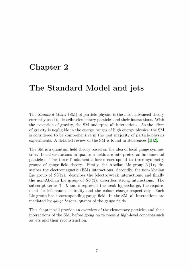
The interactions between elementary particles are mediated by the gaugebosons with spin-1. Of these, photons mediate EM interactions, W± and Zbosons are responsible for weak interactions, and the strong force is carriedby gluons. Gauge bosons may also be referred to as vector bosons, due tothe vector field they correspond to in quantum field theory. Although not agauge boson, the Higgs boson also has integral spin (spin-0) and is a scalarboson, corresponding to the scalar Higgs field. The particles of the SMis presented in Figure 2.1. The figure additionally illustrates the couplingbetween the particles.
Figure 2.1: Table of the fundamental particles of the SM (left) and a graphillustrating the coupling between the particles (right) [3, 4].
2.2 Quantum chromodynamics 9
Not all elementary particles interact with each force. Quarks experienceEM, weak and strong interactions, while leptons only experience the twofirst. Unlike quarks, leptons do not carry the color charge related to thestrong force and hence do not experience strong interactions. Strong inter-actions are at the core of proton-proton collisions and which are central tothis thesis. Therefore, strong interactions will be described in more detailin Section 2.2.
The elementary particles obtain their masses via the Higgs mechanism,which manifests experimentally as the Higgs boson. With the exceptionof neutrinos, the Higgs boson couples with and generates the masses forall fundamental particles. The mechanism behind the generation of theneutrino mass remains unknown. However it is clear that a finite massdifference between the generations must exist to allow oscillations betweenflavour eigenstates.
2.2 Quantum chromodynamics
Quantum chromodynamics (QCD) provides an effective theoretical frame-work to describe strong interactions. Strong interactions merit considera-tion due to their importance in proton-proton collisions and in the subse-quent formation of jets.
The strong force acts on the colour charge carried by quarks and gluons.Borrowing from the widely established red, blue and green colour system,the colour charge is described by red, green and blue “colours”. Conversely,the antiquarks have corresponding “anti-colours”.
QCD is based on the SU(3) gauge symmetry group and has eight gaugebosons called gluons. The non-Abelian property of the symmetry groupenables the interaction and colour exchange between the gluons them-selves. The gluon self-interaction polarizes the vacuum which consequentlyincreases the force linearly with distance greater than about a femtometer.This differs from the EM and weak forces, which become weaker as thedistance increases. As a consequence, only at very high-energy momentumtransfers, or equivalently at small distances, do quarks and gluons behavelike free or weakly bound particles. This property is called asymptotic free-dom. Another consequence is the phenomenon of colour confinement. Themutual interaction of gluons means that quarks can never exist in isolation.
10 2 The Standard Model and jets
At the separation of (anti)quarks, the potential energy necessary to over-come the colour field becomes so large that it is more energy efficient tobreak the bond by the emergence of a quark-antiquark pair out of vacuum.
2.3 Jets
Due to colour confinement, quarks and gluons cannot exist freely. Instead,they form colour-neutral hadrons in a process referred to as hadronization.No exact theory for hadronization is known, however there exist two suc-cessful models used by the event generators at CMS. Hadronization resultsin a collimated spray of particles, including hadrons as well as soft photonsand leptons originating from secondary hadron decays.
Owing to colour confinement, detection of final-state quarks and gluons isnot possible. Instead, event properties which have a close correspondencewith their distributions are studied. These event properties are known asjets. To create a jet, the final-state particles are clustered according to bestestimates of the initial-state quark or gluon from which they originated [5].
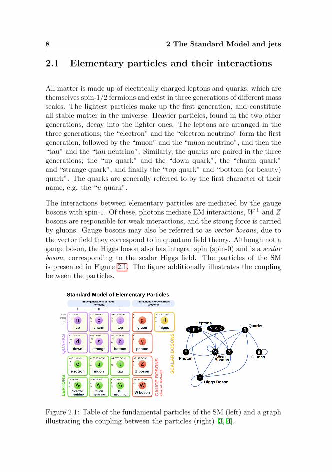
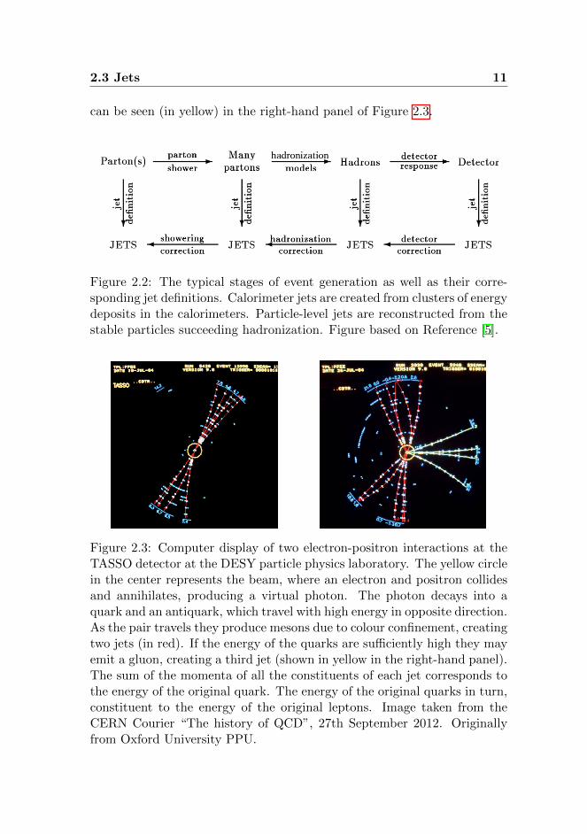
Jets are typically created from topologically-related energy deposits in thecalorimeters, some which are associated with tracks of charged particles.However, jets may be defined during all stages of the event generation(presented in the top row of Figure 2.2). Using experimentally deriveddata, calorimeter jets are created from clusters of energy deposits in thedetector’s calorimeters. From simulated data, the calorimeter jets can bereconstructed based on the simulated detector response. These two arerepresented in the right-most jet definition of the figure. Using simulateddata, jets can also be reconstructed directly from the stable particles of thecollision (simulated events contain direct information of these particles).This is represented by the next-to-last jet definition in the figure. Thesejets are referred to as particle-level jets. In this thesis, particle-level jetsare important when computing and correcting the jet response and as atool to validate the overall corrections.
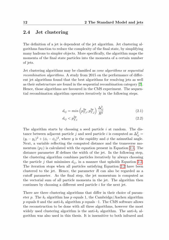
The clustering of final-state particles reduces the complexity of the eventand facilitates analysis. In addition, these clusters are helpful when study-ing QCD processes. The importance of jets can be exemplified by con-sidering the first ever detection of gluons at the TASSO detector at theDESY particle physics laboratory [6]. While gluons decay too quickly tobe detected, their fragmentation trace could be observed as a jet. This jet
2.3 Jets 11
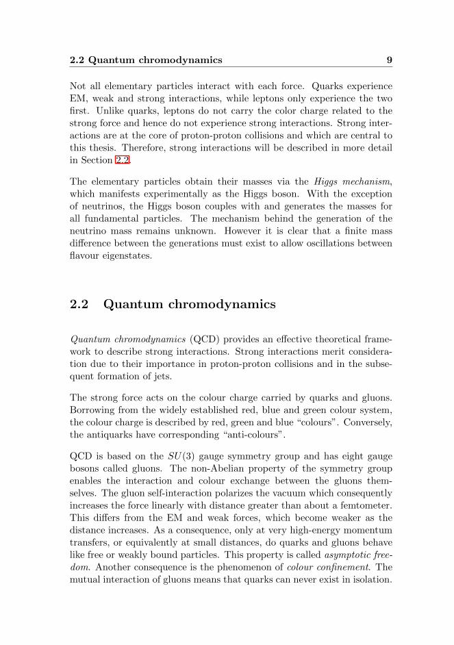
can be seen (in yellow) in the right-hand panel of Figure 2.3.
Figure 2.2: The typical stages of event generation as well as their corre-sponding jet definitions. Calorimeter jets are created from clusters of energydeposits in the calorimeters. Particle-level jets are reconstructed from thestable particles succeeding hadronization. Figure based on Reference [5].
Figure 2.3: Computer display of two electron-positron interactions at theTASSO detector at the DESY particle physics laboratory. The yellow circlein the center represents the beam, where an electron and positron collidesand annihilates, producing a virtual photon. The photon decays into aquark and an antiquark, which travel with high energy in opposite direction.As the pair travels they produce mesons due to colour confinement, creatingtwo jets (in red). If the energy of the quarks are sufficiently high they mayemit a gluon, creating a third jet (shown in yellow in the right-hand panel).The sum of the momenta of all the constituents of each jet corresponds tothe energy of the original quark. The energy of the original quarks in turn,constituent to the energy of the original leptons. Image taken from theCERN Courier “The history of QCD”, 27th September 2012. Originallyfrom Oxford University PPU.
12 2 The Standard Model and jets
2.4 Jet clustering
The definition of a jet is dependent of the jet algorithm. Jet clustering al-gorithms function to reduce the complexity of the final state, by simplifyingmany hadrons to simpler objects. More specifically, the algorithm maps themomenta of the final state particles into the momenta of a certain numberof jets.
Jet clustering algorithms may be classified as cone algorithms or sequentialrecombination algorithms. A study from 2015 on the performance of differ-ent jet algorithms found that the best algorithms for resolving jets as wellas their substructure are found in the sequential recombination category [7].Hence, those algorithms are favoured in the CMS experiment. The sequen-tial recombination algorithm operates iteratively in the following steps.
dij = min(p2pT,i, p
2pT,j
) ∆2ij
R2(2.1)
dij < p2pT,i (2.2)
The algorithm starts by choosing a seed particle i at random. The dis-tance between adjacent particle j and seed particle i is computed as ∆2
ij =
(yi − yj)2 + (φi − φj)2, where y is the rapidity and φ the azimuthal angle.Next, a variable reflecting the computed distance and the transverse mo-mentum (pT) is calculated with the equation present in Equation 2.1. Thedistance parameter R defines the width of the jet. In the following step,the clustering algorithm combines particles iteratively by always choosingthe particle j that minimises dij , in a manner that upholds Equation 2.2.The iteration stops when all particles satisfying Equation 2.2 have beenclustered to the jet. Hence, the parameter R can also be regarded as acutoff parameter. As the final step, the jet momentum is computed asthe vectorial sum of all particle momenta in the jet. The algorithm thencontinues by choosing a different seed particle i for the next jet.
There are three clustering algorithms that differ in their choice of param-eter p. The kt algorithm has p equals 1, the Cambridge/Aachen algorithmp equals 0 and the anti-kt algorithm p equals –1. The CMS software allowsthe reconstruction to be done with all three algorithms, however the mostwidely used clustering algorithm is the anti-kt algorithm. The anti-kt al-gorithm was also used in this thesis. It is insensitive to both infrared and
2.4 Jet clustering 13
collinear divergences. The former means that the addition of soft infraredparticles does not change the outcome of the clustering. The latter, thatthe addition of a collection of collinear particles with some total momentumis clustered identically to a single particle with the same momentum. Thisis necessary as to avoid bias from the threshold trigger of a calorimeter celland the background noise. The anti-kt algorithm is also largely favouredas it behaves like an idealised cone algorithm, shaping hard jets perfectlycircular on the (y, φ)-plane [8].
The anti-kT algorithm clusters all stable final-state particles (excludingneutrinos) with a decay length of cτ > 1 cm [9]. The exclusion of neu-trinos is a convention adopted by CMS, having only a small effect as theresponse is measured from samples with negligible neutrino content. How-ever, additional systematic uncertainty should be considered for measure-ments including heavy hadrons fragmentation relative to the original b andc quarks.

14 2 The Standard Model and jets
Chapter 3
Event simulation
To aid in the extraction of useful information from data recorded by thedetector, accurate models of the event kinematics at parton and parti-cle level are simulated to a high degree of accuracy. Simulated eventsare produced by general-purpose Monte Carlo event generators, such asPythia [10] and Herwig [11]. Additional software (e.g. MadGraph [12]and Powheg [13]) is commonly used to generate parton-level events. Theiroutput is subsequently directed to the two previously mentioned event gen-erators for further processing. At the CMS, simulated events are storedin the same format and reconstructed in the same way as experimentally-derived data. Simulated events are necessary in various parts of experi-mental particle physics. As presented in this thesis, simulated events areused in conjunction with detector simulation to estimate the signal andbackground of high-energy collisions.
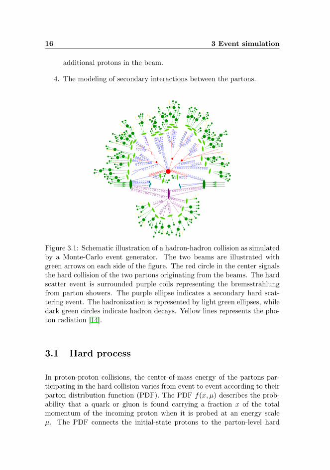
The production of proton-proton collision simulated events at the LHC canbe separated into four steps, which will be outlined in this chapter. Thesteps can be seen illustrated in Figure 3.1 and listed below:
1. The generation of the hard process, a few-body interaction which ismodeled using pertubation theory.
2. The forward and backward evolution of parton showers, which sys-tematically adjust the event towards a more realistic model.
3. The hadronization of the partons, where final-state partons are con-fined into colorless hadrons, and initial-state partons interact with
15
16 3 Event simulation
additional protons in the beam.
4. The modeling of secondary interactions between the partons.
Figure 3.1: Schematic illustration of a hadron-hadron collision as simulatedby a Monte-Carlo event generator. The two beams are illustrated withgreen arrows on each side of the figure. The red circle in the center signalsthe hard collision of the two partons originating from the beams. The hardscatter event is surrounded purple coils representing the bremsstrahlungfrom parton showers. The purple ellipse indicates a secondary hard scat-tering event. The hadronization is represented by light green ellipses, whiledark green circles indicate hadron decays. Yellow lines represents the pho-ton radiation [14].
3.1 Hard process
In proton-proton collisions, the center-of-mass energy of the partons par-ticipating in the hard collision varies from event to event according to theirparton distribution function (PDF). The PDF f(x, µ) describes the prob-ability that a quark or gluon is found carrying a fraction x of the totalmomentum of the incoming proton when it is probed at an energy scaleµ. The PDF connects the initial-state protons to the parton-level hard
3.2 Parton shower 17
process. The PDF is measured experimentally, as it is determined by thenon-perturbative physics inside the proton.
The probability amplitude of a process can be calculated by summing theterms corresponding to the Feynman diagrams up to a chosen order. Nor-mally the leading-order is sufficient to describe the main features of theprocess, although some models use next-to-leading order. The square ofthe amplitude gives the matrix element of the process, which provides in-formation about the strength of the transition between the initial- andfinal-state.
The generation of the hard process starts by selecting two partons fromthe colliding protons according to their PDFs. These are taken as theinitial-state particles for which one can calculate the matrix element andsubsequently the cross-section of the physical process. The distributionof the hard event is then predicted by theory based on the cross-section.Using the cross-section, the phase space is sampled and candidate eventsare chosen on random by a uniform distribution. As the quarks and gluonsare present as free particles in the initial- and final-state, the energy ofthe collision must be high enough for the partons to acquire asymptoticfreedom.
3.2 Parton shower
The event simulation increases in complexity as initial partons generatefinite amounts of bremsstrahlung radiation, either before or after partici-pating in the hard process. Coloured partons may emit gluons, and due tothe non-Abelian nature of QCD, gluons may also themselves emit gluons.These emissions give rise to a cascade of partons which are continuouslybeing scattered, annihilated and created until they reach the infrared cutoffat about 1 GeV [15]. The resulting cascade of partons is called a partonshower.
To model parton showers, an approximate method is formulated using prob-ability distributions for branching partons. The process results to the for-mulation of a step-wise Markov chain.
In the parton showering model the emissions are separated into initial-state radiation (ISR) and final-state radiation (FSR). ISR is showered bybackward evolution, from the hard process, in a time-reversed way towards
18 3 Event simulation
the incoming protons. Conversely, FSR evolves forward in time, creatingnew branches until reaching the infrared cutoff [16].
Event generators model parton showering in different ways. Pythia usespT-ordered dipole showers in which the hardest emissions come first. Her-wig employs angular-ordered parton showers, where the branching withlargest angles are performed first to ensure correct treatment of soft glu-ons. A more detailed description of the parton showering models and therelated calculations schemes can be found in Ref. [14].
3.3 Hadronization
When the momentum transfer reaches the previously described infraredcutoff, the perturbative QCD breaks down, and further handling of theevent is done with a non-perturbative model. This is when hadronizationhappens. Hadronization describes the process by which coloured partonsare transformed into colourless primary hadrons, which may decay in turnto secondary hadrons. Non-perturbative in nature, event generators de-scribe the transition by fine tuning free parameters according to the resultsof carefully executed experiments.
At the hadronization stage, partons are no longer treated independently,but rather as a colour connected system. The implementation of par-ton hadronization differs between event generators. Pythia applies ahadronization model commonly referred to as the Lund model. This modelis based on linear confinement (the linear growth of the potential energybetween partons of opposite charge, when separated at a distance greaterthan about a femtometer). In the Lund model, quarks are connected witha “colour string”. As the quarks become more distanced and the stringgrows, the potential energy exceeds the order of a hadron’s mass. At thispoint it becomes more energy efficient to break the string by the emer-gence of a quark-antiquark pair out of a vacuum. Herwig uses a clusterhadronization model based on preconfinement. At the end of the partonshower, all gluons are separated into quark-antiquark pairs. Next, colour-singlet combinations of partons, called clusters, are formed. These clusterssubsequently form stable hadrons, ending the generation of new partons.
3.4 Underlying event 19
3.4 Underlying event
Due to the composite nature of the LHC’s beam particles, the proton-proton collision is dominated by soft QCD events referred to as the un-derlying event. The underlying event represent all additional processes notdirectly associated with the hard interaction. Some ambiguity exists inhow the hard interaction is described, but it is commonly defined as allprocesses that occur after the associated ISR and FSR.
The main cause of the underlying event is the additional colour exchangesbetween the remnants of the colliding protons. These exchanges are mod-eled as perturbative multiple parton-parton interactions (MPI), and arehandled in a manner analogous to ISR and FSR [17]. MPI add furthercomplexity due to subsequent parton showers which may combine with theshowers from the hard interaction.
The beam contains more than a hundred billion protons per bunching, andeach proton constitute of three valence quarks and an interactive sea ofantiquarks, quarks and gluons. Not every parton participates in a hardinteraction; most take part in soft secondary interactions. The soft interac-tions consist mostly of multiple-parton interactions and diffractive scatter-ings that produce low momentum particles. As the associated momentumtransfer is low, perturbative QCD is not applicable and numerical modelsare used. The non-perturbative models use free parameters that are tunedaccording to experimental results. Eventually, particles of the underlyingevent are also subject to hadronization described in Section 3.3.
The simulated events used in this thesis are QCD multijet events, i.e. eventswith final-states consisting of a high multiplicity of jets. The events aregenerated using Pythia 8.230 with tune CP5. Modeling of the ISR, FSR,hard scattering, and MPI was done with PDFs at next-to-next-to-leadingorder (NNLO) [18]. The hard process were generated with collision energy13 TeV and the events have transverse momentum ranging from 15 to 7000GeV.

20 3 Event simulation
Chapter 4
Detector simulation
Following the previously described steps of event simulation, the simulatedevent is what an “ideal detector” would measure. In order to simulate arealistic response as the particles interact with the detector materials, thenext step is to process the event with radiation transportation software.Such software simulates the propagation of particles and their energy de-posits in the detector. The events for this thesis were processed through aCMS detector simulation based of Geant4 [19].
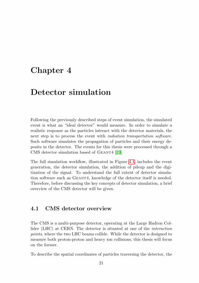
The full simulation workflow, illustrated in Figure 4.1, includes the eventgeneration, the detector simulation, the addition of pileup and the digi-tization of the signal. To understand the full extent of detector simula-tion software such as Geant4, knowledge of the detector itself is needed.Therefore, before discussing the key concepts of detector simulation, a briefoverview of the CMS detector will be given.
4.1 CMS detector overview
The CMS is a multi-purpose detector, operating at the Large Hadron Col-lider (LHC) at CERN. The detector is situated at one of the interactionpoints, where the two LHC beams collide. While the detector is designed tomeasure both proton-proton and heavy ion collisions, this thesis will focuson the former.
To describe the spatial coordinates of particles traversing the detector, the
21
22 4 Detector simulation
Figure 4.1: Illustration of the simulation workflow. After event generation,the detector response is simulated as the particles propagate through a de-tailed simulation of the CMS detector. The hard process and pileup eventsare generated separately. Both type of events are then combined beforesimulating the conversion of energy deposits to electric signals (referred toas digitization). The output of this step is known as “raw data”.
CMS experiment has adopted a right-handed coordinate system with anorigin at the beam interaction point. The plane of the x-axis points radi-ally inwards towards the center of the LHC ring, while the y-axis pointsvertically upwards (perpendicular to the plane defined by the LHC ring).The x- and y-axes span the transverse plane, where the azimuthal angle(φ) is defined. The z-axis corresponds to the longitudinal axis of the CMSdetector and points along the direction of the anticlockwise beam. Thepolar angle (θ) describes the angle of a particle with respect to the z-axis.Pseudorapidity (η) is then calculated from θ, as below.
η = −ln
(tan
θ
2
)(4.1)
η is the term commonly used to describe the angle of the particle relativeto the z-axis.
The CMS detector can be considered as comprising three regional segments
4.1 CMS detector overview 23
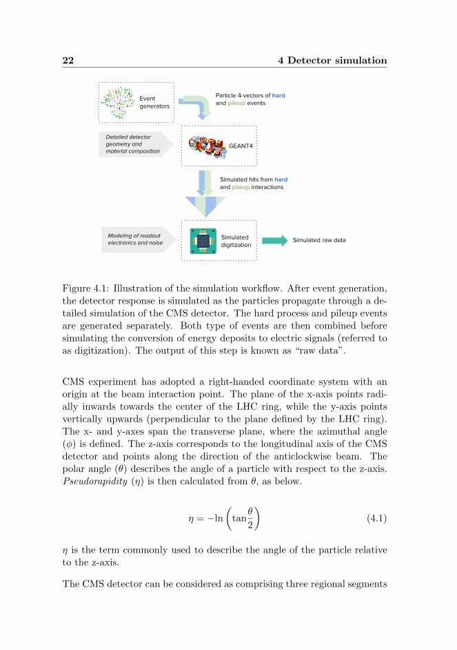
spanning different ranges of η. The barrel region describes |η| < 1.3, theendcap region 1.3 < |η| < 3.0, and the forward region 3.0 < |η| < 5.0.Additionally, the parts of the endcap region that are within and outside thetracker coverage are known as EC1 (1.3 < |η| < 2.5) and EC2 (2.5 < |η| <3) respectively. The structure of the detector is illustrated in Figure 4.2.The range of η is defined on the top and the right margins.
Figure 4.2: One quadrant of the CMS detector shown in the (z,y)-plane.The tracker, the ECAL and the HCAL (both defined in the following para-graph) are shown along with the muon chambers. The range of η is illus-trated on the top and the right margins [20].
As the barrel and endcap particles produced from the beam interactionstraverse through the detector, they pass through several layers of differentsubdetectors. The subdetectors measure the trajectories and energies ofthese particles. The subdetector closest to the interaction point is thesilicon tracker, which measures trajectories of charged particles. As seenin Figure 4.2, the tracker is surrounded by the electromagnetic calorimeter(ECAL) which functions to absorb and measure the energy of electrons andphotons. The next subdetector (the hadronic calorimeter - HCAL) absorbsand measures the energy remaining from showers initiated in ECAL, as wellas any hadronic showers initiated in the HCAL itself. A superconductingsolenoid magnet then encloses the tracker and calorimeters. The magnetprovides a strong magnetic field which bends the trajectories of chargedparticles, allowing precise measurement of their momentum and charge.
24 4 Detector simulation
Finally, multiple muon chambers alternate with layers of the return ironyoke.
In contrast to the barrel and endcap particles, particles in the forwardregion close to the beam interact with forward calorimeters.
4.2 GEANT4
All components, including active detector parts and passive materials suchas cables and cooling systems, are modeled in Geant4. The central de-tector alone (consisting of the tracker, the calorimeters and the muon sub-system) constitute of more than one million geometrical volumes [21]. De-tails about the detector geometry and material composition is provided toGeant4 with a dedicated software package. Concepts such as magneticfield type and propagation parameters are also configurable.
Geant4 simulates the particle interactions using stochastic methods. Thesoftware applies different stochastic processes depending on the probabilityof interaction. The software describes several interactions including ioniza-tion, bremsstrahlung and multiple scattering as well as detector propertiesincluding tracking, geometry description and material specifications. Themodeling of interactions extend over a large range of energies, from elasticscattering at the MeV scale to hadron showers at the GeV and TeV scale.
4.3 Pileup overlay
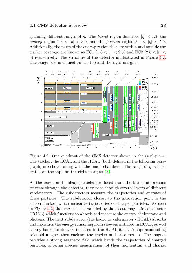
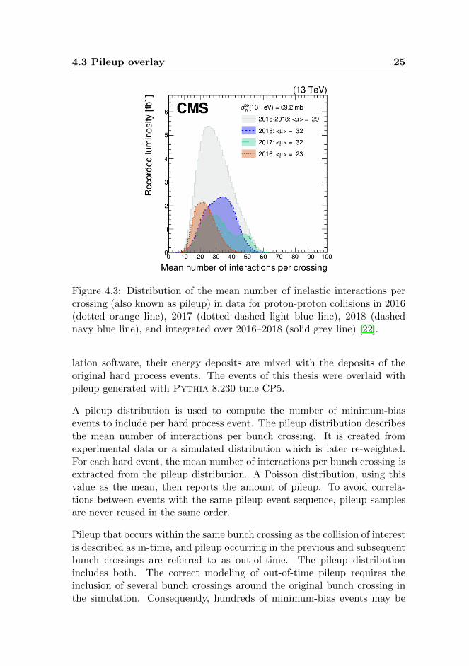
During high luminosity (L = 15 × 1033 cm−2 s−1) in 2018, LHC producesan average of about 32 inelastic proton-proton collisions per bunch cross-ing [22]. The distributions of the mean number of inelastic interactionsper crossing for the years 2016, 2017 and 2018 are presented in Figure 4.3.These additional collisions “pile up” on on top of the signal (hard scat-tering). As the simulation of pileup depends on the LHC luminosity andrun conditions, it is simulated separately from the signal. Pileup is addedto the hard process events by mixing minimum-bias events (soft QCD in-teractions with a minimum number of tracks). The minimum-bias eventsare generated and processed through the simulation steps as described inChapter 3 and Section 4.2. After being processed by the detector simu-
4.3 Pileup overlay 25
Figure 4.3: Distribution of the mean number of inelastic interactions percrossing (also known as pileup) in data for proton-proton collisions in 2016(dotted orange line), 2017 (dotted dashed light blue line), 2018 (dashednavy blue line), and integrated over 2016–2018 (solid grey line) [22].
lation software, their energy deposits are mixed with the deposits of theoriginal hard process events. The events of this thesis were overlaid withpileup generated with Pythia 8.230 tune CP5.
A pileup distribution is used to compute the number of minimum-biasevents to include per hard process event. The pileup distribution describesthe mean number of interactions per bunch crossing. It is created fromexperimental data or a simulated distribution which is later re-weighted.For each hard event, the mean number of interactions per bunch crossing isextracted from the pileup distribution. A Poisson distribution, using thisvalue as the mean, then reports the amount of pileup. To avoid correla-tions between events with the same pileup event sequence, pileup samplesare never reused in the same order.
Pileup that occurs within the same bunch crossing as the collision of interestis described as in-time, and pileup occurring in the previous and subsequentbunch crossings are referred to as out-of-time. The pileup distributionincludes both. The correct modeling of out-of-time pileup requires theinclusion of several bunch crossings around the original bunch crossing inthe simulation. Consequently, hundreds of minimum-bias events may be
26 4 Detector simulation
needed to model pileup for one generated hard event. Simulating pileup isoften the most time-consuming process.
In cases when the simulation campaign starts prior to completion of datacollection, the pileup distribution for data is unknown when simulatingpileup. To ensure event generation with small statistical uncertainty cov-ering the full kinematic phase space at the LHC, the pileup events aregenerated with a flat pT spectrum. Then, prior to analysis, the simulatedevents are re-weighted. The re-weighting matches the pileup distributionsbetween data and simulation.
4.4 Digitization
After collection, all detector energy deposits are converted to electric sig-nals during a step referred to as digitization. Digitization is performed byCMS software, simulating the behavior of the readout electronics used inexperimental data acquisition. To obtain a realistic detector response thesimulation includes electronic noise.
Each subdetector has dedicated software for simulating the electronic read-out response. Charged particles traversing the active elements of the tracker,distributes energy loss along their trajectory. Therefore, the signal model-ing of the tracker readouts include Landau fluctuations as well as Lorentzdrift and diffusion of charges to the detector surface. The modeling also ac-counts for noise and coupling between channels. Since the process is similarin all the calorimeter subsystems, digitization of calorimeter signals use aunified framework. Modeling of ECAL and HCAL takes particular care insimulating the efficiency and non-uniformity in the photon collection of thecrystals and modules. To correctly simulate overlay of out-of-time pileupwith the signal, the model simulates signal pulses as a function of time pereach hit. In the muon drift tubes, focus is put on the particle directionand impact position with respect to the sense wire. Due to air gaps wheredetectors are placed within the iron yoke, modeling of the muon detectoraccounts for the residual magnetic field effects this creates [23].
At this stage, the simulation of Level-1 trigger electronics is added. Thesimulated events are stored in a format identical to that used for experimen-tal data. Similar to data, each simulated event contains the information ofthe Level-1 trigger it would have passed if it were a real event. This allowsfor the use of the same reconstruction algorithms and tools in simulated

4.4 Digitization 27
and experimentally-derived data.

28 4 Detector simulation
Chapter 5
Event reconstruction
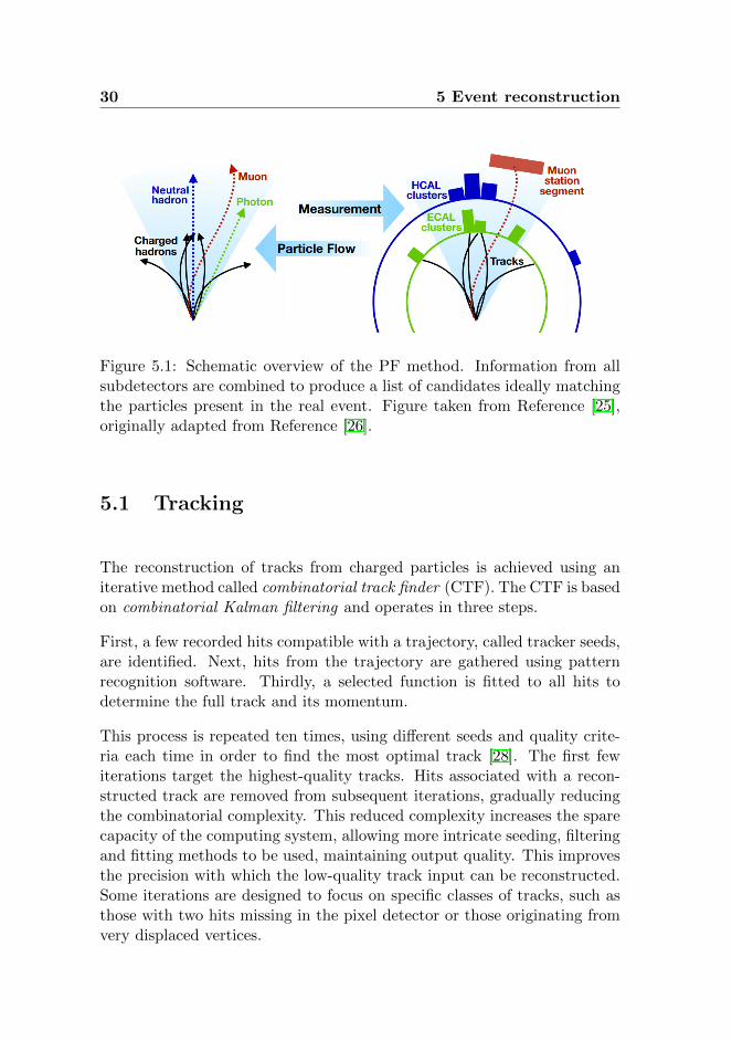
Following event and detector simulation, each event is reconstructed usingthe particle-flow (PF) algorithm [24]. The purpose is to bring the recordedpicture of the collision event back to particle-level. Combining informationfrom all subdetectors, the goal is to reconstruct each type of particle sep-arately. This requires the matching of tracks and energy clusters betweenthe tracker and calorimeters. This combinatorial approach, illustrated inFigure 5.1, provides a more accurate event reconstruction than if relyingon a single detector. The PF algorithm aims for a complete global eventdescription. This includes a list of all particles present in the event andtheir properties such as charges, trajectories, and momenta.
The output of the PF algorithm is a set of PF candidates, classified intoelectrons, muons, photons, and charged and neutral hadrons. Hadronsand photons are further clustered into jets. Some jets may additionally beidentified as originating from b quark hadronization or from hadronicallydecaying tau leptons. The presence of weakly interacting neutral particlesis identified by calculating the missing transverse momentum of the event.
The PF approach was originally designed in the ALEPH experiment, whichrecorded the positron-electron collisions at the LEP [27]. The CMS nowwidely uses the PF method when reconstructing events. The PF methodbenefits from the CMS experiment due to the increased precision in chargedhadron measurements, arising from the highly segmented ECAL. In addi-tion, the muon tracking system provides an excellent muon identification.The stages of event reconstruction using the PF method will now be dis-cussed.
29
30 5 Event reconstruction
Figure 5.1: Schematic overview of the PF method. Information from allsubdetectors are combined to produce a list of candidates ideally matchingthe particles present in the real event. Figure taken from Reference [25],originally adapted from Reference [26].
5.1 Tracking
The reconstruction of tracks from charged particles is achieved using aniterative method called combinatorial track finder (CTF). The CTF is basedon combinatorial Kalman filtering and operates in three steps.
First, a few recorded hits compatible with a trajectory, called tracker seeds,are identified. Next, hits from the trajectory are gathered using patternrecognition software. Thirdly, a selected function is fitted to all hits todetermine the full track and its momentum.
This process is repeated ten times, using different seeds and quality crite-ria each time in order to find the most optimal track [28]. The first fewiterations target the highest-quality tracks. Hits associated with a recon-structed track are removed from subsequent iterations, gradually reducingthe combinatorial complexity. This reduced complexity increases the sparecapacity of the computing system, allowing more intricate seeding, filteringand fitting methods to be used, maintaining output quality. This improvesthe precision with which the low-quality track input can be reconstructed.Some iterations are designed to focus on specific classes of tracks, such asthose with two hits missing in the pixel detector or those originating fromvery displaced vertices.
5.2 Calorimeter clustering 31
5.2 Calorimeter clustering
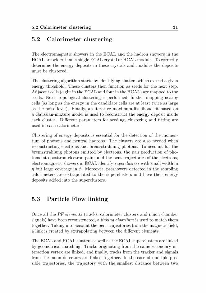
The electromagnetic showers in the ECAL and the hadron showers in theHCAL are wider than a single ECAL crystal or HCAL module. To correctlydetermine the energy deposits in these crystals and modules the depositsmust be clustered.
The clustering algorithm starts by identifying clusters which exceed a givenenergy threshold. These clusters then function as seeds for the next step.Adjacent cells (eight in the ECAL and four in the HCAL) are mapped to theseeds. Next, topological clustering is performed, further mapping nearbycells (as long as the energy in the candidate cells are at least twice as largeas the noise level). Finally, an iterative maximum-likelihood fit based ona Gaussian-mixture model is used to reconstruct the energy deposit insideeach cluster. Different parameters for seeding, clustering and fitting areused in each calorimeter.
Clustering of energy deposits is essential for the detection of the momen-tum of photons and neutral hadrons. The clusters are also needed whenreconstructing electrons and bremsstrahlung photons. To account for thebremsstrahlung photons emitted by electrons, the pair production of pho-tons into positron-electron pairs, and the bent trajectories of the electrons,electromagnetic showers in ECAL identify superclusters with small width inη but large coverage in φ. Moreover, preshowers detected in the samplingcalorimeters are extrapolated to the superclusters and have their energydeposits added into the superclusters.
5.3 Particle Flow linking
Once all the PF elements (tracks, calorimeter clusters and muon chambersignals) have been reconstructed, a linking algorithm is used to match themtogether. Taking into account the bent trajectories from the magnetic field,a link is created by extrapolating between the different elements.
The ECAL and HCAL clusters as well as the ECAL superclusters are linkedby geometrical matching. Tracks originating from the same secondary in-teraction vertex are linked, and finally, tracks from the tracker and signalsfrom the muon detectors are linked together. In the case of multiple pos-sible trajectories, the trajectory with the smallest distance between two
32 5 Event reconstruction
elements is kept.
Sudden emission of bremsstrahlung in the tracker can change the directionof the electron trajectories. To improve the quality of reconstruction, theelectron candidates (tracks linked to ECAL superclusters) are refitted witha Gaussians-sum filter algorithm, taking into account the possible energylosses due to bremsstrahlung. In addition, a dedicated algorithm takes careof tracking photons to potential positron-electron pairs arising from pairproduction.
Once the links have been made, PF blocks are created. Each PF block isa collection of elements linked together by association of the same singleparticle or group of particles. The identification and reconstruction of PFcandidates is carried out in each PF block separately.
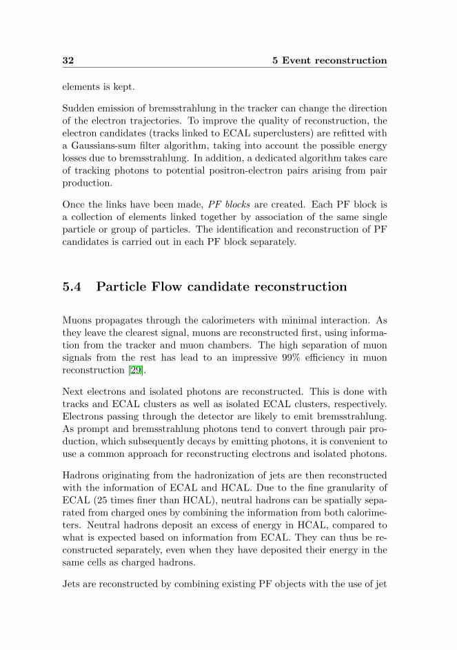
5.4 Particle Flow candidate reconstruction
Muons propagates through the calorimeters with minimal interaction. Asthey leave the clearest signal, muons are reconstructed first, using informa-tion from the tracker and muon chambers. The high separation of muonsignals from the rest has lead to an impressive 99% efficiency in muonreconstruction [29].
Next electrons and isolated photons are reconstructed. This is done withtracks and ECAL clusters as well as isolated ECAL clusters, respectively.Electrons passing through the detector are likely to emit bremsstrahlung.As prompt and bremsstrahlung photons tend to convert through pair pro-duction, which subsequently decays by emitting photons, it is convenient touse a common approach for reconstructing electrons and isolated photons.
Hadrons originating from the hadronization of jets are then reconstructedwith the information of ECAL and HCAL. Due to the fine granularity ofECAL (25 times finer than HCAL), neutral hadrons can be spatially sepa-rated from charged ones by combining the information from both calorime-ters. Neutral hadrons deposit an excess of energy in HCAL, compared towhat is expected based on information from ECAL. They can thus be re-constructed separately, even when they have deposited their energy in thesame cells as charged hadrons.
Jets are reconstructed by combining existing PF objects with the use of jet
5.5 Jet reconstruction 33
algorithms (such as the anti-kT algorithm explained in Section 2.4). ThePF algorithm is very useful as it allows jets to be presented as a collectionof individual constituents, compared to a single object. Finally, weakly in-teracting neutral particles are determined by calculating the missing trans-verse momentum, which first relies on the reconstruction of all PF objectsin the event.
5.5 Jet reconstruction
Different types of jets are created in the CMS experiment. The type of jetdepends on the method of reconstruction, which differ by the use of differentkinds of detector inputs and reconstruction algorithms. The different jetsare the following:
• PF jets are reconstructed from particle-flow candidates.
• PFchs jets are reconstructed from particle-flow candidates where charged-hadron substraction (CHS) has been performed. CHS is explainedfurther in Section 6.1.1.
• PFPuppi jets are reconstructed from particle-flow candidates usingthe pileup per particle identification (PUPPI) algorithm. PUPPI isexplained further in Section 6.1.1.
• Calo jets are reconstructed by solely utilising the energy deposits fromthe calorimeters.
• JPT jets are reconstructed by combining the charged particle tracksto the spatially associated Calo jets.
An important parameter governing any algorithm is the jet distance param-eter, which specifies the size of a cone-shaped jet in the (η, φ)-plane. Theparameter is specified as R =
√(∆η2 + ∆φ2). The default jet distance pa-
rameters for Run 2 are 0.4 and 0.8. At the CMS, jet distance parameter 0.4is mainly used for reconstruction of showers from light quarks. Conversely,0.8 is used for heavy particles such as W, Z, Higgs bosons and beyond SMparticles created with a large Lorentz boost. The particles decays of heavyboosted particles are often very collinear. This makes jet reconstructiondifficult when using a small jet distance parameter and hence it is better toreconstruct all decay products within one jet with a larger size of 0.8 [22].

34 5 Event reconstruction
The reconstructed jets typically have the shorthand names [AA][CS][TY],where [AA] represents the clustering algorithm, [CS] represents the jet dis-tance parameter and the [TY] represents the jet type. Resulting namesinclude AK4PFchs or AK8PFPuppi.
Chapter 6
Jet Energy Correction
As the jets traverse through the CMS detector, signals are left in the de-tector components. The individual signals are combined to PF candidates,which jet algorithms use to produce reconstructed jets. However, due to anarray of effects, the energy of the reconstructed jets do not precisely equalthe particle-level jet energies.
The discrepancies between PF and particle-level jets arise from various ef-fects, including energy deposits from pileup interactions, non-linear calorime-ter response to hadrons, minimum energy thresholds in calorimeters andnuclear interactions in the tracker material. To account for and correctfor these differences, jets are calibrated via a sequential multi-step process.The steps facilitate the correction of the effects of pileup, the non-lineardetector response, the residual simulation-data jet energy scale (JES) dif-ferences and the flavour biased differences. The two first steps are appliedto both simulated events and experimentally-derived data. The third stepis only applied to data, in an attempt to bring it closer to the simulation.The fourth step is optional in both cases. As this thesis focuses on derivingcorrections from simulation, only the two first steps are further discussedin Chapter 8 and 9.
The computed corrections are applied as scale factors for the jet four-momentum, factors which depend on various jet related quantities suchas jet pT, η and area Ajet, as well as the pileup pT offset density ρ in theevent. Finally, closure tests contribute to the validation of the corrections.Within simulated jets, corrections are derived separately for the PF, PFchs,Puppi, Calo and JPT jets. Conversely, the residual corrections derived from
35
36 6 Jet Energy Correction
experimental data are computed specifically for PFchs jets (with R = 0.4)and assumed to be the same for all other kind of jets.
The JES is critical to many physics analyses, and its precision makes animportant contribution to their systematic uncertainties. In addition tocomparing the jet cross-section to QCD predictions, accurate jet measure-ments are important for a variety of processes such as calibrating high-massparticles decaying to quarks and gluons, removing soft contamination fromhard jets, tagging heavy objects originating from jets and for backgroundsubtraction. A better understanding of the JES and its uncertainties allowsfor more precise analysis measurements.
6.1 Pileup offset corrections
The additional contribution of jet energy and momentum due to pileup isreferred to as pileup offset. The pileup offset correction adjusts the energyby estimating and then removing the energy corresponding to pileup in-side the jet. Pileup removal is performed with both experimentally-deriveddata and simulated events. This chapter will consider two different ap-proaches of pileup mitigation; that performed at per-particle level beforejet clustering (CHS, PUPPI [22]), and at per-jet level after jet clustering(area-median [9]).
6.1.1 Pileup mitigation before jet clustering
The two most widely used methods within the CMS experiment operatingat the PF candidate level are the CHS and the PUPPI method. Unlike theCHS method, which rejects only charged particles associated with pileupvertices, PUPPI applies a more rigorous selection to charged particles aswell as rescales the four-momenta of neutral particles according to theirprobability of originating from the primary collision of interest, the leadingvertex (LV). Both methods act on the particles, complementing the pileupsubtraction algorithms performed after jet clustering (see Section 6.1.2)which work at the event or jet level. The pileup-corrected particles emergingfrom both CHS and PUPPI are used as input to jet clustering algorithms.CHS clustered jets are further corrected for residual neutral offset by theevent or jet level pileup mitigation algorithms, while no such correction isnecessary for PUPPI jets.
6.1 Pileup offset corrections 37
In CHS, charged particles originating from pileup vertices are identifiedand removed from the event. Charged hadrons are identified in the PFalgorithm as tracks, which are associated with calorimeter hits. The LVis chosen based on the largest sum of squares of the track transverse mo-menta [22]. Subleading vertices are classified as pileup vertices, and arerequired to pass further quality criteria based on a minimum number ofdegrees of freedom in the vertex fit. If the track of a charged hadron is as-sociated with a pileup vertex satisfying the above criteria, it is consideredas pileup and removed.
The PUPPI algorithm builds on the CHS algorithm. The addition is basedon the observation that neutral particles from a parton shower are typicallyaligned with charged particles from the same shower, while the particlesfrom pileup vertices are more uniformly distributed in all directions.
The PUPPI algorithm operates as follows. Firstly, charged particles areassigned weights based on their available tracking information. Particlesused in the fit of the LV are assigned a weight of 1, while those associatedwith a pileup vertex are assigned a weight of 0. Next, the algorithm definesa local metric α which differs between leading and pileup vertices. Thevariable α is constructed to be large for particles close to the LV, and forparticles with |η| > 2.5, to be close to highly energetic particles [22]. AtCMS the variable α for a given particle i is defined in Equation 6.1. Here,variable j are all other particles at a distance Rij less or equal to R0 = 0.4,pT,j their transverse momentum in GeV and ∆Rij =
√(∆η2
ij + ∆φ2ij). In
|η| < 2.5 where tracking information is available, only charged particlesassociated with the LV are considered. Finally, the unique α-distributionsfor leading and pileup vertices are computed.
αi = log∑
j 6=i,∆Rij<R0
(pT,j
∆Rij
)2
{for |ηi| < 2.5, j are charged particles originating from the LV,
for |ηi| > 2.5, j are other reconstructed particles,
(6.1)
The algorithm uses the α-distributions for charged particles considered aspileup, to generate expected event-level pileup distributions. The weightsof neutral particles are assigned by comparing their α values to the medianand root-mean-squared (RMS) of the charged pileup distribution. Smallweights encode the probability that the particle originated from pileup.
38 6 Jet Energy Correction
Finally, the weights are used to rescale the neutral particles four-momentato correct for pileup at particle-level. Particles with very small rescaled pT
are discarded.
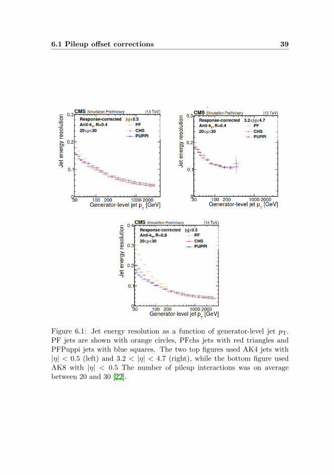
Figure 6.1 shows the jet energy resolution (JER) as a function of jet pT forPF, PFchs and PFPuppi jets. PF jets perform worse at low pT as the jetsin that region are greatly affected by pileup. In the forward region (3.2 <|η| < 4.7), where no tracking is available, PFchs jets perform the same asPF jets. PFPuppi jets are superior when R = 0.8, as neutral particles frompileup contribute greatly to such jets. The preferred algorithm depends onthe analysis. Better pileup mitigation is achieved with PUPPI comparedto CHS, especially for events with more than 30 interactions. While thePUPPI algorithm provides a better jet pT-resolution for jets with pT < 100GeV, CHS is superior when pT exceeds 100 GeV [22].
6.1.2 Pileup mitigation after jet clustering
Following the optional per-particle pileup mitigation, particles are clus-tered into jets and pileup removal on event and jet-level is performed. Thepileup offset correction is taken from the true offset in simulation, and forexperimental data the correction is further scaled by the ratio of randomcone (RC) offsets for experimental data and simulation. This will now beconsidered in more detail.
Firstly, QCD multijet events are simulated both with and without pileupoverlay. Generally, the latter sample is completely without pileup. How-ever, due to misconfiguration for samples with 〈µ〉 equal to 0, in this thesisas sample with 〈µ〉 about 10−8 was used. Particle-level jets in both sam-ples are matched, required to be within a distance less than R/2 [9]. Here,R is the jet distance parameter. Next, the particle-level pileup offset iscalculated as the average difference in pT between the matched jets. Toparametrize the pileup dependence, the diffuse offset energy density of theevent is estimated as the median of energy deposits in η/φ bins encompass-ing the whole detector. Finally, the diffuse pileup offset energy per eventis estimated. The corrections are applied as a function of the uncorrectedjet pT, η, ρ and jet area defined as the (η, φ)-plane where the particles areclustered.
For experimental data, the corrections are further scaled by offset scale fac-tors. These factors are determined with the RC method in simulated and
6.1 Pileup offset corrections 39
Figure 6.1: Jet energy resolution as a function of generator-level jet pT.PF jets are shown with orange circles, PFchs jets with red triangles andPFPuppi jets with blue squares. The two top figures used AK4 jets with|η| < 0.5 (left) and 3.2 < |η| < 4.7 (right), while the bottom figure usedAK8 with |η| < 0.5 The number of pileup interactions was on averagebetween 20 and 30 [22].
40 6 Jet Energy Correction
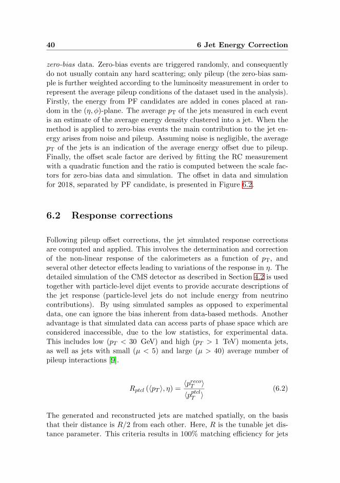
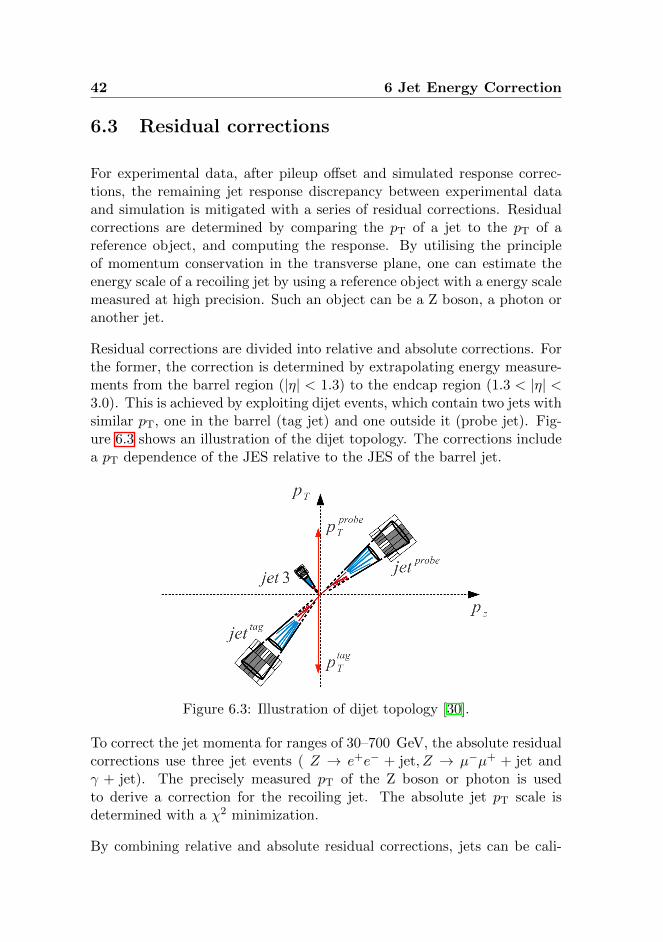
zero-bias data. Zero-bias events are triggered randomly, and consequentlydo not usually contain any hard scattering; only pileup (the zero-bias sam-ple is further weighted according to the luminosity measurement in order torepresent the average pileup conditions of the dataset used in the analysis).Firstly, the energy from PF candidates are added in cones placed at ran-dom in the (η, φ)-plane. The average pT of the jets measured in each eventis an estimate of the average energy density clustered into a jet. When themethod is applied to zero-bias events the main contribution to the jet en-ergy arises from noise and pileup. Assuming noise is negligible, the averagepT of the jets is an indication of the average energy offset due to pileup.Finally, the offset scale factor are derived by fitting the RC measurementwith a quadratic function and the ratio is computed between the scale fac-tors for zero-bias data and simulation. The offset in data and simulationfor 2018, separated by PF candidate, is presented in Figure 6.2.
6.2 Response corrections
Following pileup offset corrections, the jet simulated response correctionsare computed and applied. This involves the determination and correctionof the non-linear response of the calorimeters as a function of pT, andseveral other detector effects leading to variations of the response in η. Thedetailed simulation of the CMS detector as described in Section 4.2 is usedtogether with particle-level dijet events to provide accurate descriptions ofthe jet response (particle-level jets do not include energy from neutrinocontributions). By using simulated samples as opposed to experimentaldata, one can ignore the bias inherent from data-based methods. Anotheradvantage is that simulated data can access parts of phase space which areconsidered inaccessible, due to the low statistics, for experimental data.This includes low (pT < 30 GeV) and high (pT > 1 TeV) momenta jets,as well as jets with small (µ < 5) and large (µ > 40) average number ofpileup interactions [9].
Rptcl (〈pT 〉, η) =〈precoT 〉〈pptclT 〉
(6.2)
The generated and reconstructed jets are matched spatially, on the basisthat their distance is R/2 from each other. Here, R is the tunable jet dis-tance parameter. This criteria results in 100% matching efficiency for jets
6.2 Response corrections 41
Figure 6.2: The RC offset measured in data (markers) and simulation (his-tograms) versus η is shown on the top. The offset is normalized by the av-erage number of pileup interactions 〈µ〉. Different types of PF candidatesare represented. Associated charged hadrons are associated with recon-structed pileup vertices and thus removed from the list of PF candidates inthe jet clustering by the CHS algorithm. In contrast, unassociated chargedhadrons are not mitigated by CHS. At the bottom, the ratio of data oversimulation, representing the offset scale factor applied for pileup in data, isalso shown for PF and PFchs [30].
with pT above around 30 GeV [9]. After matching the jets, the momentumresponse is computed with Equation 6.2, where 〈precoT 〉 is the mean pT of
the reconstructed jets in a given pptclT bin, and 〈pptclT 〉 is the mean of theparticle-level jet pT in the same bin. Finally, the correction is determinedby fitting a function to the inverse of the mean response as a function of〈precoT 〉 in fine bins of η.
42 6 Jet Energy Correction
6.3 Residual corrections
For experimental data, after pileup offset and simulated response correc-tions, the remaining jet response discrepancy between experimental dataand simulation is mitigated with a series of residual corrections. Residualcorrections are determined by comparing the pT of a jet to the pT of areference object, and computing the response. By utilising the principleof momentum conservation in the transverse plane, one can estimate theenergy scale of a recoiling jet by using a reference object with a energy scalemeasured at high precision. Such an object can be a Z boson, a photon oranother jet.
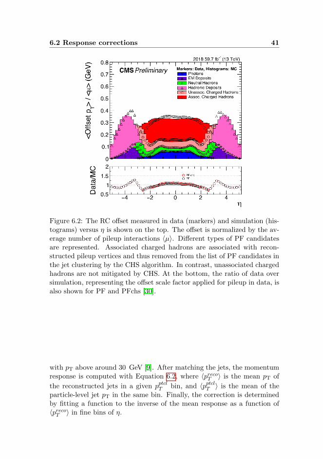
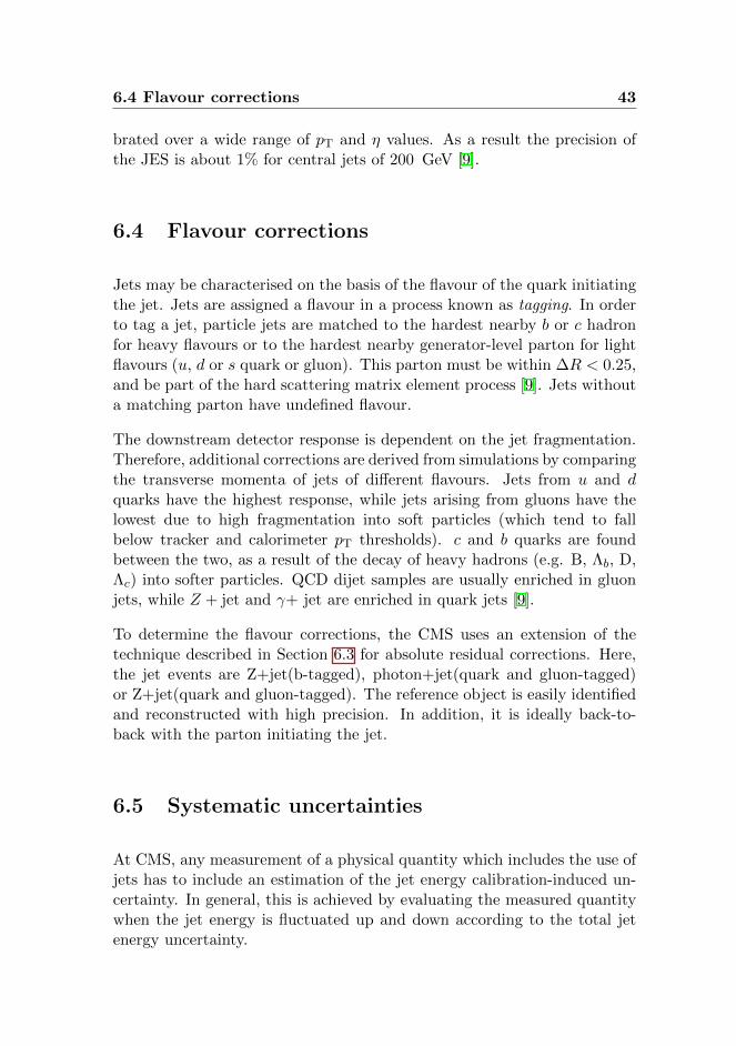
Residual corrections are divided into relative and absolute corrections. Forthe former, the correction is determined by extrapolating energy measure-ments from the barrel region (|η| < 1.3) to the endcap region (1.3 < |η| <3.0). This is achieved by exploiting dijet events, which contain two jets withsimilar pT, one in the barrel (tag jet) and one outside it (probe jet). Fig-ure 6.3 shows an illustration of the dijet topology. The corrections includea pT dependence of the JES relative to the JES of the barrel jet.
Figure 6.3: Illustration of dijet topology [30].
To correct the jet momenta for ranges of 30–700 GeV, the absolute residualcorrections use three jet events ( Z → e+e− + jet, Z → µ−µ+ + jet andγ + jet). The precisely measured pT of the Z boson or photon is usedto derive a correction for the recoiling jet. The absolute jet pT scale isdetermined with a χ2 minimization.
By combining relative and absolute residual corrections, jets can be cali-
6.4 Flavour corrections 43
brated over a wide range of pT and η values. As a result the precision ofthe JES is about 1% for central jets of 200 GeV [9].
6.4 Flavour corrections
Jets may be characterised on the basis of the flavour of the quark initiatingthe jet. Jets are assigned a flavour in a process known as tagging. In orderto tag a jet, particle jets are matched to the hardest nearby b or c hadronfor heavy flavours or to the hardest nearby generator-level parton for lightflavours (u, d or s quark or gluon). This parton must be within ∆R < 0.25,and be part of the hard scattering matrix element process [9]. Jets withouta matching parton have undefined flavour.
The downstream detector response is dependent on the jet fragmentation.Therefore, additional corrections are derived from simulations by comparingthe transverse momenta of jets of different flavours. Jets from u and dquarks have the highest response, while jets arising from gluons have thelowest due to high fragmentation into soft particles (which tend to fallbelow tracker and calorimeter pT thresholds). c and b quarks are foundbetween the two, as a result of the decay of heavy hadrons (e.g. B, Λb, D,Λc) into softer particles. QCD dijet samples are usually enriched in gluonjets, while Z + jet and γ+ jet are enriched in quark jets [9].
To determine the flavour corrections, the CMS uses an extension of thetechnique described in Section 6.3 for absolute residual corrections. Here,the jet events are Z+jet(b-tagged), photon+jet(quark and gluon-tagged)or Z+jet(quark and gluon-tagged). The reference object is easily identifiedand reconstructed with high precision. In addition, it is ideally back-to-back with the parton initiating the jet.
6.5 Systematic uncertainties
At CMS, any measurement of a physical quantity which includes the use ofjets has to include an estimation of the jet energy calibration-induced un-certainty. In general, this is achieved by evaluating the measured quantitywhen the jet energy is fluctuated up and down according to the total jetenergy uncertainty.
44 6 Jet Energy Correction
The JES uncertainties are provided as systematic sources that include cor-relations across pT and η. At CMS the total uncertainty of the jet energycorrection is computed as a quadratic sum of the uncertainty of each differ-ent source (of which there are currently 15). The uncertainties arise fromthe modeling of physics phenomena such as showers and underlying events,the modeling of the detector properties such as response and noise, andas potential biases in the methodologies used to estimate the corrections.Several of these uncertainties are related and can be combined into thefollowing groups:
• Pileup offset.
• η-relative calibration of JES.
• pT-relative calibration of JES.
• Jet flavour response.
• Time dependence.
Each of these are discussed in the following.
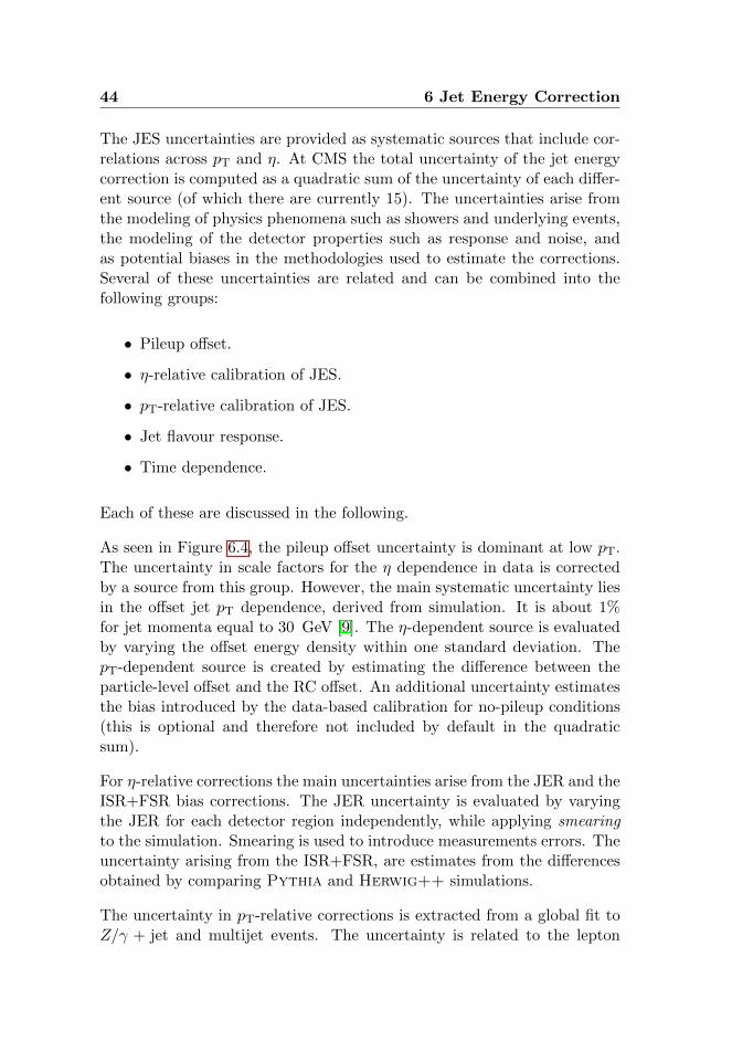
As seen in Figure 6.4, the pileup offset uncertainty is dominant at low pT.The uncertainty in scale factors for the η dependence in data is correctedby a source from this group. However, the main systematic uncertainty liesin the offset jet pT dependence, derived from simulation. It is about 1%for jet momenta equal to 30 GeV [9]. The η-dependent source is evaluatedby varying the offset energy density within one standard deviation. ThepT-dependent source is created by estimating the difference between theparticle-level offset and the RC offset. An additional uncertainty estimatesthe bias introduced by the data-based calibration for no-pileup conditions(this is optional and therefore not included by default in the quadraticsum).
For η-relative corrections the main uncertainties arise from the JER and theISR+FSR bias corrections. The JER uncertainty is evaluated by varyingthe JER for each detector region independently, while applying smearingto the simulation. Smearing is used to introduce measurements errors. Theuncertainty arising from the ISR+FSR, are estimates from the differencesobtained by comparing Pythia and Herwig++ simulations.
The uncertainty in pT-relative corrections is extracted from a global fit toZ/γ + jet and multijet events. The uncertainty is related to the lepton
6.5 Systematic uncertainties 45
momentum scale for muons in Z(→ µµ) + jet and the single-pion responsein ECAL and HCAL. Additional uncertainty is added to correct for thebias arising from the exclusion of neutrinos and ISR outside of the detectoracceptance. Shape uncertainties for the pT dependence are additionallycomputed as the jet response differences due to the different fragmentationmodels implemented in Pythia and Herwig++.
Following pileup offset uncertainties, the flavour uncertainty is the high-est at low pT (about 1.5%). The flavor uncertainties are assigned basedon Pythia and Herwig++ differences, which are propagated through amockup of the data-based calibration chain with dijet and Z/γ+jet events.The uncertainty is computed from uds/c/b-quark and gluon responses [30].The flavor differences in Pythia and Herwig++ are largest for gluon jets,while the two simulations agree well on both light-quark and heavy-flavourjets.
The JES in the endcaps shows some residual difference between the luminosity-weighted average of corrections per data-taking period per year. Prescaledtriggers samples from different run periods with different weights leadsto slight scale differences between different data sets. This time depen-dence uncertainty is estimated as the root-mean-squared variation of theη-dependent correction factors determined with dijet events, from approx-imately ten different data-taking periods [9].
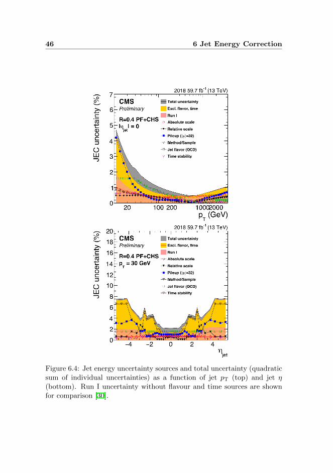
46 6 Jet Energy Correction
Figure 6.4: Jet energy uncertainty sources and total uncertainty (quadraticsum of individual uncertainties) as a function of jet pT (top) and jet η(bottom). Run I uncertainty without flavour and time sources are shownfor comparison [30].
Chapter 7
Analysis reproducibility andsoftware practices
Previous chapters discussed how high energy physicists rely heavily on largedata sets and as a result require a lot of computational power. Typically,each analysis group builds their analytical pipeline of computational stepsby using scripting languages such as Bash [31] and Python [32]. Thesepipelines are often hard to maintain, lack portability and may be difficultto compare to other pipelines. A further problem is that the pipelines lacka description of either the environment or the software packages used. Thisreduces, or completely prevents, reproducibility of the analysis in a differentcontext.
This approach uses the imperative paradigm. Here, the analyst is respon-sible for changing the state of the program by using explicit statements.In this thesis the benefits of an approach in which the description of thecontrol flow (i.e. the order and execution of the individual statements) isremoved from the analyst responsibility will be presented. This is referredto as the declarative paradigm.
Declarative rather than imperative programming enables the analyst tofocus on the solving the task without having to spend time implement-ing details such as job orchestration. The analyst’s focus is therefore onexpressing what should be executed, without focusing on how to executeit. As a result, the computational tasks of the analysis are automated andthe productivity of the analyst is improved. A further benefit of declarativeprogramming is the separation of physics knowledge from specific program-
47
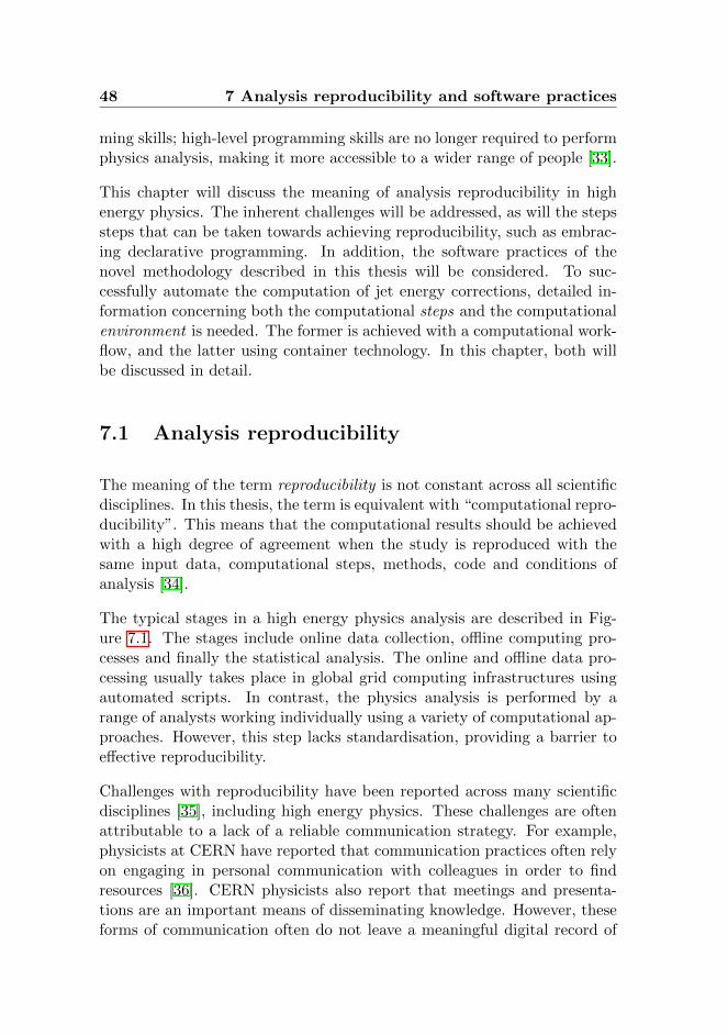
48 7 Analysis reproducibility and software practices
ming skills; high-level programming skills are no longer required to performphysics analysis, making it more accessible to a wider range of people [33].
This chapter will discuss the meaning of analysis reproducibility in highenergy physics. The inherent challenges will be addressed, as will the stepssteps that can be taken towards achieving reproducibility, such as embrac-ing declarative programming. In addition, the software practices of thenovel methodology described in this thesis will be considered. To suc-cessfully automate the computation of jet energy corrections, detailed in-formation concerning both the computational steps and the computationalenvironment is needed. The former is achieved with a computational work-flow, and the latter using container technology. In this chapter, both willbe discussed in detail.
7.1 Analysis reproducibility
The meaning of the term reproducibility is not constant across all scientificdisciplines. In this thesis, the term is equivalent with “computational repro-ducibility”. This means that the computational results should be achievedwith a high degree of agreement when the study is reproduced with thesame input data, computational steps, methods, code and conditions ofanalysis [34].
The typical stages in a high energy physics analysis are described in Fig-ure 7.1. The stages include online data collection, offline computing pro-cesses and finally the statistical analysis. The online and offline data pro-cessing usually takes place in global grid computing infrastructures usingautomated scripts. In contrast, the physics analysis is performed by arange of analysts working individually using a variety of computational ap-proaches. However, this step lacks standardisation, providing a barrier toeffective reproducibility.
Challenges with reproducibility have been reported across many scientificdisciplines [35], including high energy physics. These challenges are oftenattributable to a lack of a reliable communication strategy. For example,physicists at CERN have reported that communication practices often relyon engaging in personal communication with colleagues in order to findresources [36]. CERN physicists also report that meetings and presenta-tions are an important means of disseminating knowledge. However, theseforms of communication often do not leave a meaningful digital record of
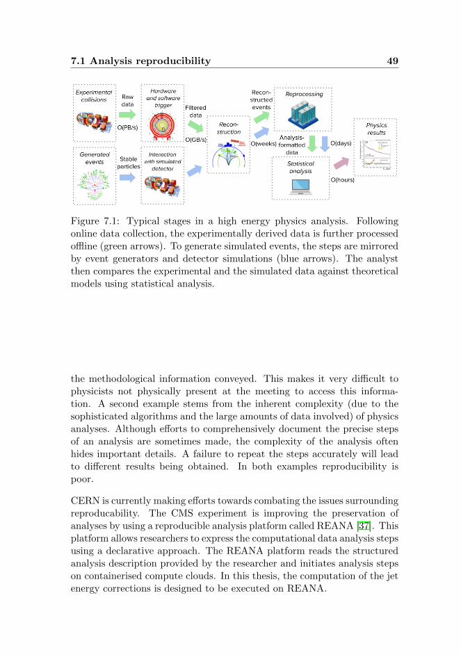
7.1 Analysis reproducibility 49
Figure 7.1: Typical stages in a high energy physics analysis. Followingonline data collection, the experimentally derived data is further processedoffline (green arrows). To generate simulated events, the steps are mirroredby event generators and detector simulations (blue arrows). The analystthen compares the experimental and the simulated data against theoreticalmodels using statistical analysis.
the methodological information conveyed. This makes it very difficult tophysicists not physically present at the meeting to access this informa-tion. A second example stems from the inherent complexity (due to thesophisticated algorithms and the large amounts of data involved) of physicsanalyses. Although efforts to comprehensively document the precise stepsof an analysis are sometimes made, the complexity of the analysis oftenhides important details. A failure to repeat the steps accurately will leadto different results being obtained. In both examples reproducibility ispoor.
CERN is currently making efforts towards combating the issues surroundingreproducability. The CMS experiment is improving the preservation ofanalyses by using a reproducible analysis platform called REANA [37]. Thisplatform allows researchers to express the computational data analysis stepsusing a declarative approach. The REANA platform reads the structuredanalysis description provided by the researcher and initiates analysis stepson containerised compute clouds. In this thesis, the computation of the jetenergy corrections is designed to be executed on REANA.
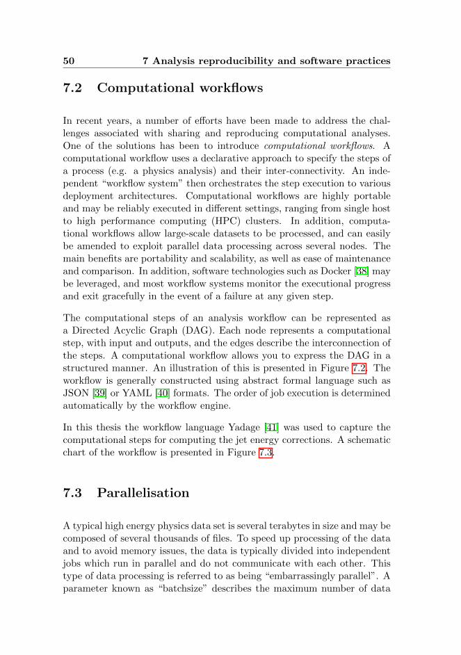
50 7 Analysis reproducibility and software practices
7.2 Computational workflows
In recent years, a number of efforts have been made to address the chal-lenges associated with sharing and reproducing computational analyses.One of the solutions has been to introduce computational workflows. Acomputational workflow uses a declarative approach to specify the steps ofa process (e.g. a physics analysis) and their inter-connectivity. An inde-pendent “workflow system” then orchestrates the step execution to variousdeployment architectures. Computational workflows are highly portableand may be reliably executed in different settings, ranging from single hostto high performance computing (HPC) clusters. In addition, computa-tional workflows allow large-scale datasets to be processed, and can easilybe amended to exploit parallel data processing across several nodes. Themain benefits are portability and scalability, as well as ease of maintenanceand comparison. In addition, software technologies such as Docker [38] maybe leveraged, and most workflow systems monitor the executional progressand exit gracefully in the event of a failure at any given step.
The computational steps of an analysis workflow can be represented asa Directed Acyclic Graph (DAG). Each node represents a computationalstep, with input and outputs, and the edges describe the interconnection ofthe steps. A computational workflow allows you to express the DAG in astructured manner. An illustration of this is presented in Figure 7.2. Theworkflow is generally constructed using abstract formal language such asJSON [39] or YAML [40] formats. The order of job execution is determinedautomatically by the workflow engine.
In this thesis the workflow language Yadage [41] was used to capture thecomputational steps for computing the jet energy corrections. A schematicchart of the workflow is presented in Figure 7.3.
7.3 Parallelisation
A typical high energy physics data set is several terabytes in size and may becomposed of several thousands of files. To speed up processing of the dataand to avoid memory issues, the data is typically divided into independentjobs which run in parallel and do not communicate with each other. Thistype of data processing is referred to as being “embarrassingly parallel”. Aparameter known as “batchsize” describes the maximum number of data
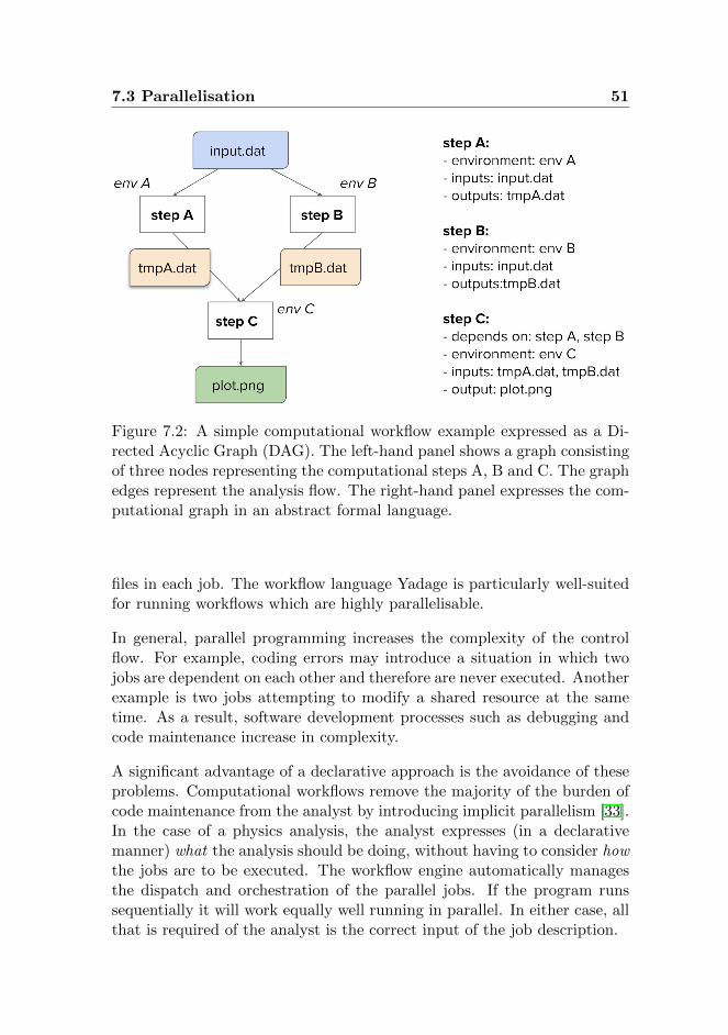
7.3 Parallelisation 51
Figure 7.2: A simple computational workflow example expressed as a Di-rected Acyclic Graph (DAG). The left-hand panel shows a graph consistingof three nodes representing the computational steps A, B and C. The graphedges represent the analysis flow. The right-hand panel expresses the com-putational graph in an abstract formal language.
files in each job. The workflow language Yadage is particularly well-suitedfor running workflows which are highly parallelisable.
In general, parallel programming increases the complexity of the controlflow. For example, coding errors may introduce a situation in which twojobs are dependent on each other and therefore are never executed. Anotherexample is two jobs attempting to modify a shared resource at the sametime. As a result, software development processes such as debugging andcode maintenance increase in complexity.
A significant advantage of a declarative approach is the avoidance of theseproblems. Computational workflows remove the majority of the burden ofcode maintenance from the analyst by introducing implicit parallelism [33].In the case of a physics analysis, the analyst expresses (in a declarativemanner) what the analysis should be doing, without having to consider howthe jobs are to be executed. The workflow engine automatically managesthe dispatch and orchestration of the parallel jobs. If the program runssequentially it will work equally well running in parallel. In either case, allthat is required of the analyst is the correct input of the job description.
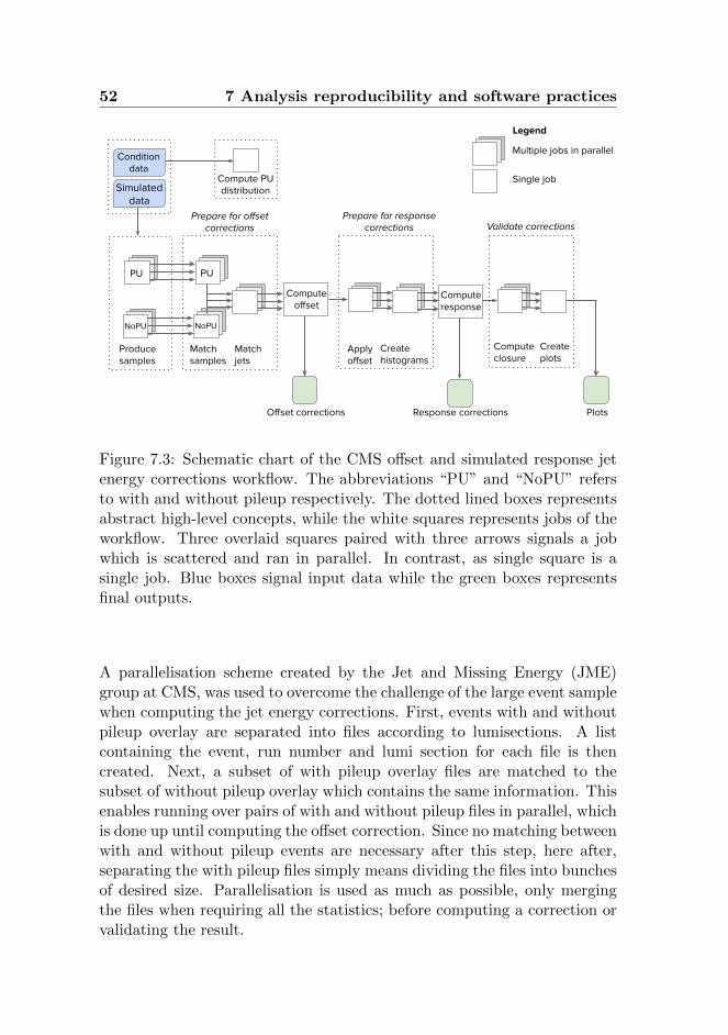
52 7 Analysis reproducibility and software practices
Figure 7.3: Schematic chart of the CMS offset and simulated response jetenergy corrections workflow. The abbreviations “PU” and “NoPU” refersto with and without pileup respectively. The dotted lined boxes representsabstract high-level concepts, while the white squares represents jobs of theworkflow. Three overlaid squares paired with three arrows signals a jobwhich is scattered and ran in parallel. In contrast, as single square is asingle job. Blue boxes signal input data while the green boxes representsfinal outputs.
A parallelisation scheme created by the Jet and Missing Energy (JME)group at CMS, was used to overcome the challenge of the large event samplewhen computing the jet energy corrections. First, events with and withoutpileup overlay are separated into files according to lumisections. A listcontaining the event, run number and lumi section for each file is thencreated. Next, a subset of with pileup overlay files are matched to thesubset of without pileup overlay which contains the same information. Thisenables running over pairs of with and without pileup files in parallel, whichis done up until computing the offset correction. Since no matching betweenwith and without pileup events are necessary after this step, here after,separating the with pileup files simply means dividing the files into bunchesof desired size. Parallelisation is used as much as possible, only mergingthe files when requiring all the statistics; before computing a correction orvalidating the result.
7.4 Container technology 53
7.4 Container technology
The capture of the computational steps of an analysis is not in itself ad-equate for effective reproducibility. Computational analyses are designedand run in a specific computing environment. Reproducibility problemsmay arise as documentation of an environment is often insufficient to ac-curately replicate the environment for future analyses. As a solution, con-tainer technology may be used to capture the computational environmentas well as necessary software packages.
Virtual machines (VM) have been used to simulate computing environmentssince the 1960s [42]. VMs are software which allows functional emulationof a specific physical computer on a different computer. Containers arelightweight counterparts to VMs, offering virtualization at the operatingsystem level as opposed to the hardware level. Containers allow the pack-aging of an application, with its dependencies, so that it can be run inisolation from other processes. Container technology enables the analystto work in a computing environment that has been frozen with respect tothe libraries and conditions of the analysis. As a result, the analyst canuse the same software that analysts were using several years ago withouthaving to download all the relevant years-old libraries.
Two widely adopted open source container technologies are Docker andSingularity [43]. The former is used for development, testing, and deploy-ment across various software enterprises, while the latter was specificallydesigned for HPC clusters.
Containers are powerful additions to computational workflows as they pack-age the precise computational components required to execute each step.For instance, containers ensure that the step performing data selection hasthe necessary data selection libraries installed, while the step requiring spe-cific CMS SoftWare (CMSSW) has access to the necessary release. Furtherinformation regarding containerizing CMSSW is provided in Appendix A.Another major benefit is the portability that containers provide. Analystscan download containers and recreate the analysis environment on theirown system, data center or cloud provider.
In this thesis a lightweight Docker image only containing the base operatingsystem (Centos7) was used. Cern VM File System (CVMFS) was mountedduring run time to access CMSSW for compiling the code and for execution.
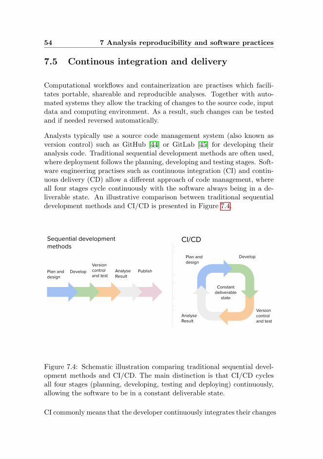
54 7 Analysis reproducibility and software practices
7.5 Continous integration and delivery
Computational workflows and containerization are practises which facili-tates portable, shareable and reproducible analyses. Together with auto-mated systems they allow the tracking of changes to the source code, inputdata and computing environment. As a result, such changes can be testedand if needed reversed automatically.
Analysts typically use a source code management system (also known asversion control) such as GitHub [44] or GitLab [45] for developing theiranalysis code. Traditional sequential development methods are often used,where deployment follows the planning, developing and testing stages. Soft-ware engineering practises such as continuous integration (CI) and contin-uous delivery (CD) allow a different approach of code management, whereall four stages cycle continuously with the software always being in a de-liverable state. An illustrative comparison between traditional sequentialdevelopment methods and CI/CD is presented in Figure 7.4.
Figure 7.4: Schematic illustration comparing traditional sequential devel-opment methods and CI/CD. The main distinction is that CI/CD cyclesall four stages (planning, developing, testing and deploying) continuously,allowing the software to be in a constant deliverable state.
CI commonly means that the developer continuously integrates their changes
7.5 Continous integration and delivery 55
with the main codebase. This is achieved by automating the compilationand test phases of the workflow. The system is configured to automaticallyperform the tasks after the integration of code changes [46]. In so doing,one may avoid challenges that can occur when when integration is delayed.CD is an extension of CI. CD ensures that the software is always ready tobe released [47].
The main benefits of CI/CD are avoiding errors as the coding mistakesare identified early by the automated tests. This allows the developerto spend less time testing and solving issues, leaving more time for codeimprovement. In addition, CI allows the analyst to often and automaticallyexamine how changes in the source code, input data and computationalenvironment affects the output.
For these reasons, CI/CD have gained widespread popularity in the soft-ware industry. However, despite these benefits it has not yet been adoptedby most physicists. The CMS experiment has a lifespan of decades, includescoding contributions from a large number of developers and is constantlybeing upgraded to achieve higher precision. Due to the lack of standardi-sation of the individual analyses within the wider CMS experiment, intro-ducing CI/CD would greatly increase coding efficiencies, minimise the needfor manual testing and maintain code quality.
REANA has developed a GitLab-REANA bridge that allows researchersto use GitLab as the source code management platform to develop theirworkflows, and REANA as a CI service to run them. The jet calibrationworkflow of this thesis was developed in hand with this integration.

56 7 Analysis reproducibility and software practices
Chapter 8
Results
In this chapter further details are presented about the simulated samplesthat were used when computing the jet energy corrections discussed in thisthesis. The average value of the ratio of measured jet pT to particle-leveljet pptclT is referred to as the response. As a ratio close to one indicates awell calibrated jet, the response is used to validate the computed energycorrection. The response of the computed corrections are presented, as arethe benefits of automating the computation. The corrections are computedfor jets with two different jet distance parameters (R=0.4 and R=0.8).There is also a consideration of the benefits of using a declarative, ratherthan imperative, paradigm.
8.1 Sample description
The main input to the workflow were two simulated QCD multijet samples(with and without pileup overlaid), each consisting of tens of millions ofevents. Both samples had a size of a few terabytes. The first step of thepreparatory phase consists of matching particle-level jets to PF jets. Inthis step, a preliminary filter is applied to the data in order to extractonly information which is useful for downstream analysis. This speedsup the analysis. This step is typically split into several hundred parallelcomputing jobs, each lasting several hours, and is performed with specifictools implemented in CMSSW. The output of this preparatory phase isan analysis formatted sample which has a reduced size of a few hundredgigabytes. This step is summarised in the two first rows of Table 8.1.
57
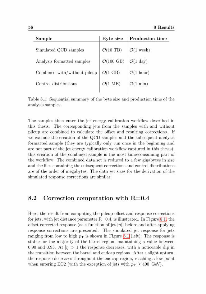
58 8 Results
Sample Byte size Production time
Simulated QCD samples O(10 TB) O(1 week)
Analysis formatted samples O(100 GB) O(1 day)
Combined with/without pileup O(1 GB) O(1 hour)
Control distributions O(1 MB) O(1 min)
Table 8.1: Sequential summary of the byte size and production time of theanalysis samples.
The samples then enter the jet energy calibration workflow described inthis thesis. The corresponding jets from the samples with and withoutpileup are combined to calculate the offset and resulting corrections. Ifwe exclude the creation of the QCD samples and the subsequent analysisformatted sample (they are typically only run once in the beginning andare not part of the jet energy calibration workflow captured in this thesis),this creation of the combined sample is the most time-consuming part ofthe workflow. The combined data set is reduced to a few gigabytes in sizeand the files containing the subsequent corrections and control distributionsare of the order of megabytes. The data set sizes for the derivation of thesimulated response corrections are similar.
8.2 Correction computation with R=0.4
Here, the result from computing the pileup offset and response correctionsfor jets, with jet distance parameter R=0.4, is illustrated. In Figure 8.1, theoffset-corrected response (as a function of jet |η|) before and after applyingresponse corrections are presented. The simulated jet response for jetsranging from low to high pT is shown in Figure 8.1 (left). The response isstable for the majority of the barrel region, maintaining a value between0.90 and 0.95. At |η| > 1 the response decreases, with a noticeable dip inthe transition between the barrel and endcap regions. After a slight upturn,the response decreases throughout the endcap region, reaching a low pointwhen entering EC2 (with the exception of jets with pT ≥ 400 GeV).
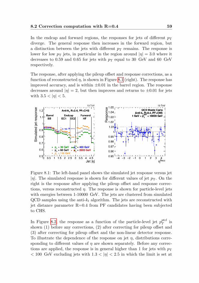
8.2 Correction computation with R=0.4 59
In the endcap and forward regions, the responses for jets of different pT
diverge. The general response then increases in the forward region, buta distinction between the jets with different pT remains. The response islower for low pT jets, in particular in the region around |η| = 3.0 where itdecreases to 0.59 and 0.65 for jets with pT equal to 30 GeV and 60 GeVrespectively.
The response, after applying the pileup offset and response corrections, as afunction of reconstructed η, is shown in Figure 8.1 (right). The response hasimproved accuracy, and is within ±0.01 in the barrel region. The responsedecreases around |η| = 2, but then improves and returns to ±0.01 for jetswith 3.5 < |η| < 5.
Figure 8.1: The left-hand panel shows the simulated jet response versus jet|η|. The simulated response is shown for different values of jet pT. On theright is the response after applying the pileup offset and response correc-tions, versus reconstructed η. The response is shown for particle-level jetswith energies between 1-10000 GeV. The jets are clustered from simulatedQCD samples using the anti-kt algorithm. The jets are reconstructed withjet distance parameter R=0.4 from PF candidates having been subjectedto CHS.
In Figure 8.2, the response as a function of the particle-level jet pptclT isshown (1) before any corrections, (2) after correcting for pileup offset and(3) after correcting for pileup offset and the non-linear detector response.To illustrate the dependence of the response on jet η, distributions corre-sponding to different values of η are shown separately. Before any correc-tions are applied, the response is in general higher than 1 for jets with pT
< 100 GeV excluding jets with 1.3 < |η| < 2.5 in which the limit is set at
60 8 Results
about 30 GeV. After correcting for pileup offset, jets with 2.5 < |η| < 3.0have a noticeably lower response. The response for these jets reaches 0.56as the pT decreases. After correcting for both pileup offset and the non-linear detector response, the jet response is stable for jets with pT in theranges from 30 to 2000 GeV. For jets with pT < 30 GeV, excluding jetswith 2.5 < |η| < 3.0, the response stays within ±0.05. For jets with2.5 < |η| < 3.0 the response decreases as the jet pT decreases, finallyreaching 0.79.
8.3 Correction computation with R=0.8
Here, the results from computing the pileup offset and response corrections,for jets with jet distance parameter R=0.8, are illustrated. The simulatedjet response for jets ranging from low to high pT (Figure 8.3, left) willbe considered first. As with R=0.4, the detector response is stable for themajority of the barrel region, remaining between 0.90 and 0.95 for jets withpT ≥ 60 GeV. Similarly to R=0.4, in the endcap and forward regions theresponse diverges for jets with different pT. However, for R=0.8, there isalready a noticeable divergence in the barrel region for jets with low pT.Again, there is a slight dip in the transition between the barrel and endcapregions. Similarly to R=0.4, the response in generally lower for low pT jets.The response in the forward region follows a similar curve as for R=0.4.
The response, after applying the pileup offset and response corrections (Fig-ure 8.3, right), is also similar to that of R=0.4. The response is within±0.01in the barrel region. However in contrast to R=0.4, the response remainswithin that limit for longer, up to |η| < 4. Additionally, the barrel andendcap regions are characterised by reduced response variation.
The response at different stages of the workflow (Figure 8.4) are now con-sidered. Before applying the corrections the response is higher than 1 forjets with pT < 100 GeV. This is similar to the results for R=0.4, but alsoincludes jets with 1.3 < |η| < 2.5). Similarly to R=0.4, after computingand correcting for pileup offset, jets within 2.5 < |η| < 3.0 have the lowestresponse (reaching 0.60 at pT equal to 0 GeV). After correcting for bothpileup offset and the non-linear detector response, the jet response is stablefor jets with pT in the ranges 50− 2000 GeV. For jets with pT < 50 GeVthe response decreases with pT, decreasing to 0.85 for jets in the barrel andendcap region, and 0.57 for jets with 2.5 < |η| < 3.0.
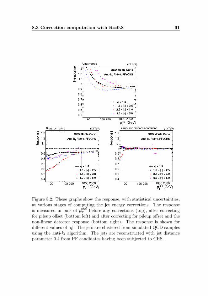
8.3 Correction computation with R=0.8 61
Figure 8.2: These graphs show the response, with statistical uncertainties,at various stages of computing the jet energy corrections. The responseis measured in bins of pptclT before any corrections (top), after correctingfor pileup offset (bottom left) and after correcting for pileup offset and thenon-linear detector response (bottom right). The response is shown fordifferent values of |η|. The jets are clustered from simulated QCD samplesusing the anti-kt algorithm. The jets are reconstructed with jet distanceparameter 0.4 from PF candidates having been subjected to CHS.
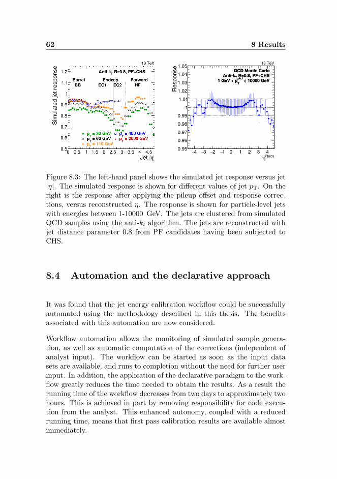
62 8 Results
4− 3− 2− 1− 0 1 2 3 4Recoη
0.950.960.970.980.99
11.011.021.031.041.05
Res
pons
e
13 TeV
QCD Monte CarloR=0.8, PF+CHSTAnti-k
< 10000 GeVptclT
1 GeV < p
QCD Monte CarloR=0.8, PF+CHSTAnti-k
< 10000 GeVptclT
1 GeV < p
Figure 8.3: The left-hand panel shows the simulated jet response versus jet|η|. The simulated response is shown for different values of jet pT. On theright is the response after applying the pileup offset and response correc-tions, versus reconstructed η. The response is shown for particle-level jetswith energies between 1-10000 GeV. The jets are clustered from simulatedQCD samples using the anti-kt algorithm. The jets are reconstructed withjet distance parameter 0.8 from PF candidates having been subjected toCHS.
8.4 Automation and the declarative approach
It was found that the jet energy calibration workflow could be successfullyautomated using the methodology described in this thesis. The benefitsassociated with this automation are now considered.
Workflow automation allows the monitoring of simulated sample genera-tion, as well as automatic computation of the corrections (independent ofanalyst input). The workflow can be started as soon as the input datasets are available, and runs to completion without the need for further userinput. In addition, the application of the declarative paradigm to the work-flow greatly reduces the time needed to obtain the results. As a result therunning time of the workflow decreases from two days to approximately twohours. This is achieved in part by removing responsibility for code execu-tion from the analyst. This enhanced autonomy, coupled with a reducedrunning time, means that first pass calibration results are available almostimmediately.
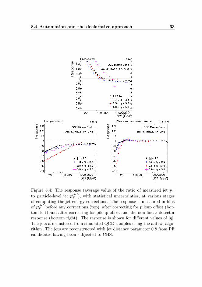
8.4 Automation and the declarative approach 63
Figure 8.4: The response (average value of the ratio of measured jet pT
to particle-level jet pptclT ), with statistical uncertainties, at various stagesof computing the jet energy corrections. The response is measured in binsof pptclT before any corrections (top), after correcting for pileup offset (bot-tom left) and after correcting for pileup offset and the non-linear detectorresponse (bottom right). The response is shown for different values of |η|.The jets are clustered from simulated QCD samples using the anti-kt algo-rithm. The jets are reconstructed with jet distance parameter 0.8 from PFcandidates having been subjected to CHS.
64 8 Results
Another result is the increased ease of code maintenance. The compu-tational steps are saved with the environment in one place under versioncontrol. Source code changes, changes to the job description and changes tothe computational environment are all automatically saved and versionedbetween runs. This brings improved reproducibility. With the additionof CI, the analyst is able to test changes at any stage. This allows, forexample, the analyst to take into account an improved parameterisation.The restarted workflows are versioned and do not overwrite previous it-erations, thereby conserving the full provenance of results and facilitatingcomparisons between previous runs.
However, it is worth noting that this method is not without its challenges.As with all physics analyses, the analyst typically rerun workflows manytimes with altered conditions, either to fix a problem or to study the re-sults with altered parameters. With this new automated approach, manualintervention is still required to do this.
Chapter 9
Discussion
The results of the thesis are discussed in detail. Firstly, the similarities anddifferences between the computed jet response for jet distance parameterR=0.4 and R=0.8 will be considered. Secondly, the advantages to automat-ing the jet energy calibration workflow will be presented. This will includethe benefits of shifting from the imperative to the declarative paradigm. Fi-nally, potential sociological and technological challenges to the widespreadadoption of automated declarative analyses will be discussed.
9.1 Comparing corrections with R=0.4 and R=0.8
Examining the response figures for R=0.4 and R=0.8, it is clear that thegeneral structure for both cases follows the same curve. As seen in Fig-ure 8.1 (left) and 8.3 (left), in the barrel and endcap regions, there is ageneral trend of decreasing jet response as |η| increases. With increasing|η|, the distance which the particles have to travel through the tracker, andcorrespondingly the amount of material traversed, increases. As a result, athigher |η|, there is a greater chance of particles decaying before depositingtheir energy in the calorimeters, leading to a decrease in the response. Thedetector performance is particularly poor in the transition regions. Thereason is again the larger amount of material in front of the calorimeters,and the correspondingly high rates of nuclear interactions in the tracker. Asthe EC2 region (2.5 < |η| < 3.0) is outside tracker coverage, the responsedecreases due to a lack of tracks to be used by event reconstruction.
65
66 9 Discussion
Although the pattern for the jet response when R=0.8 is broadly similar tothat of R=0.4, there are a few differences suggesting a dependence betweenthe jet response and the jet distance parameter R. Jets with larger distanceparameter tend to contain a larger fraction of low-energy particles. Low-energy particles have a lower response compared to particles from hardscatter, lowering the response for low pT jets with large R. This can beseen in Figure 8.1 (left) and 8.3 (left). Comparing jets of 30 GeV in bothfigures, the response for jets with R=0.8 is about 0.85 throughout the barrelregion, while jets with R=0.4 is at 0.9. A similar, but less severe, effect canbe seen for jets of 60 GeV. In contrast, the high pT jets are not affectedby the jet distance parameter, staying at 0.95 in both cases.
Before correcting, the measured jet pT is greater than the particle-level jetpptclT for low pT jets with both R=0.4 and R=0.8. This can be seen in thetop of Figure 8.2 and 8.4. This is largely due to low energy pileup. Whencomparing the top and bottom left figures of Figure 8.2 and 8.4 the responseafter applying pileup-offset corrections give the biggest improvements inaccuracy for jets with pT < 100 GeV (R=0.4) and pT < 400 GeV (R=0.8).The observed difference between jets of different R is again explained bythe increased amount of particles from pile-up covered by the larger jetarea.
The larger the R, the larger the area in (η, φ)-plane that is covered by thejet. As an effect, larger jet distance parameters average the jet responseover a larger area. As a result, sharp features in the detector responseversus η are smeared. This can be seen in Figure 8.1 (right) and 8.3 (right).Comparing the two figures, the response for jets with R=0.4 appear morespread out, while the response for jets with R=0.8 follow a smooth curve.
9.2 Benefits of automation and the declarativeapproach
The results obtained from the automation of the jet energy calibrationworkflow strongly suggests that capturing complex experimental particlephysics analyses with declarative workflow languages is both achievable andadvantageous. The main benefits are that the workflow is quick, portable,scalable, and easy to maintain and compare to previous versions.
The reduced running time was expected, and may be explain by two fac-
9.2 Benefits of automation and the declarative approach 67
tors. Firstly, by automating the code execution, the workflow can be per-formed independently of the analyst. This speeds the analysis as it canprogress without the need to wait for analyst input, which may be delayedif the analyst is working on another task or it is out of working hours.The running time is also enhanced because of improved resource availabil-ity. In the established approach, the analyst dispatches jobs to computingservers through HTCondor. The HTCondor system is widely used, lead-ing to queueing times which are often significant, slowing the analysis. Incontrast, the jet energy calibration workflow described in the thesis runsin the REANA cluster. At the time of writing (February 2021) the RE-ANA cluster has 10 nodes and 80 cores available. The traffic on REANAis relatively low, greatly reducing the waiting time before the analysis canbegin and increasing the analysis speed. On REANA, the workflow runswith an average of two hours. Secondly, it is also possible to introduce afurther automated step to initiate the analysis pipeline. By monitoring thegeneration of the simulated samples (e.g. with a cron job) the correctioncomputation may be automatically started and ran to completion with-out analyst input. This removes any lag-time between simulated samplegeneration and beginning of the analysis.
The resulting reduced run time provides quick feedback on the data setquality to the CMS collaboration, enhancing the efficiency of the experi-ment.
The declarative approach further reduces workload of the analyst. Changesto the job orchestration is eased by the help of the computational work-flow. To give one example, with the computational workflow of this thesis,changing the input only requires changing the path at one place in thescript. This is true even when the number of files changes. In contrast,with an imperative approach, changing the number of files might affect theinterconnection between downstream jobs, requiring more code handling.The reduced workload frees up time for the analyst. Instead of repeatedlyrunning the largely technical and tedious parts of work, the analyst’s timecan be allocated to improving the analysis.
As discussed in Section 7.1, to help ensure the reproducibility of compu-tational results, clear and complete information about any computationalmethods, data and conditions that support the published results shouldbe shared. In our case, reproducibility is facilitated by keeping the fulldescription of these in one place. The computational steps and associatedparameters are stored and versioned by storing the computational workflow
68 9 Discussion
under version control. The computational environment where the analysiswas originally executed, such as operating system and library dependenciesare saved with the use of container technology. In addition to reproducingthe final result, any intermediate results and outputs are guaranteed withthe complete analysis pipeline captured by the computational workflow.
9.3 Challenges of automation and the declarativeapproach
The current common practice of experimental particle physicists is cen-tered around the imperative approach rather than declarative. While thereare clear advantages to the new declarative approach, there may be a fewobstacles to its widespread adoption. Despite requiring less extensive pro-gramming skills compared to the established approach, declarative pro-gramming does require the analyst to think differently about the problemat hand. The use of declarative programming necessitates more than simplylearning a new software tool, it requires a new way to structure the wholeanalysis. This may lead to some initial resistance from analysts. However,once the extensive benefits of declarative programming are understood, weanticipate the analysts to buy in to this approach.
Additional challenges foreseen by us are more technological in nature. Asdescribed in Chapter 8, manual intervention is still necessary when rerun-ning workflows. This is common practice when considering the effects ofdifferent conditions. The non-automated and imperative nature of the es-tablished approach allows the process to be restarted partway through,without the need to return to the beginning. This is desirable as the initialsteps are often the most time-consuming. This is because the data setsmust first be filtered to only contain information relevant for the down-stream analysis and converted to a simplified data format, which enablesfaster analysis. In contrast, the automated declarative approach requiresthe entire process to be repeated to obtain new results. The duplicativeand redundant rerunning of analyses represents an inefficiency of the cur-rent state of the automated declarative approach. It is possible to manuallyintervene to avoid the need to return to the start of the analysis. However,this process is more difficult than it is in the imperative approach. Futuredevelopment addressing this issue will facilitate wide-spread adoption ofthis methodology.
Chapter 10
Conclusion
This thesis describes the successful automation of the CMS jet energy cor-rections (derived from simulation) computations. This was achieved usingthe declarative paradigm, as opposed to the more commonly used impera-tive paradigm. While the widespread adoption of this new approach mustovercome anticipated challenges of a sociological and technological nature,these are considered surmountable in light of the extensive benefits.
The workflow description and containerisation allowed preservation of thecomputational tasks of the analysis together with the full description of thejob orchestration and the execution environment. Accompanying sourcecode management facilitated easier code maintenance, enhanced analystproductivity and simple comparisons between runs. Additionally, the widerdeclarative approach brought the benefits of reduced analysis running timeand increased analysis portability and scalability. Importantly, higher levelsof reproducibility were facilitated. In conclusion, automation of the jetcalibration has the potential to enhance productivity and free the analystto spend more time improving the corrections. This can lead to a betterunderstanding of the JES and its uncertainties, facilitating more precisedownstream analysis measurements and improving the CMS experiment asa whole.
69

70 10 Conclusion

Appendices
71

Appendix A
CMSSW Docker image buildingservice
The CERN Open Data portal uses virtual machines (VMs) to provide ac-cess to CMS-specific software and conditions. VMs with CMS SoftWare(CMSSW) facilitate execution reproducibility on machines without accessto the framework. VMs are often used for educational purposes, for exampleby teachers and students at workshop events. As container technology hasbecome more popular, there has been a movement towards system-agnosticcontainerized versions of CMSSW. Containers are more light-weight thanVMs and therefore require less allocated space and download time. Themain advantage of containerized versions of CMSSW mirrors that of VMs;they provide an interface facilitating access to computing tools for workingwith CMS data. Additional benefits include allowing:
• Teachers and students to avoid the need to spend hours setting upthe necessary software, often for use in a short lesson.
• Easy management of the environment and dependencies when run-ning on the batch system.
• Developing of analysis in a self-contained environment.
• Offline development.
• Access to CERN VM File System (CVMFS).
• Shared common setup between developers of larger projects.
73
74 A CMSSW Docker image building service
• Analysis preservation and reproducibility.
We created a platform for building Docker containers, with installed CMSSWreleases, on demand. The CMSSW Docker image building service (cmssw-docker.web.cern.ch/) is a part of the HEPContainers project. The goal of thisproject is to converge all HEP containers into one place, making it easy forphysicists in the HEP community to use and distribute containers createdspecifically for their kind of work.
The platform has a frontend created in REACT and backend coded inGolang. The platform avoids the need for a database by utilising GitLab.When a request is made in the frontend by the user, a HTTP request tothe backend is made. The backend utilises the GitLab API to create anGitlab issue, storing the necessary information. This include, the CMSSWrelease, SCRAM ARCH version, reason for request and email of the re-quester (if entered). The issue (request) stays open until approved. Theadministrators of the site approves the request by interacting with the issue(more exactly by adding the label “Approved”). A webhook, triggered bythe event, then provides the backend with the information of the requestedimage. The information is parsed and the GitLab API is used to start apipeline on the GitLab CI. A tool known as kaniko is responsible for build-ing the container images. Building of the image may take few hours untilcompletion. When the status of the pipeline changes, a HTTP request ismade to the backend via another webhook. If the build is successful therequester is provided with an email for how to access the requested Dockerimage. In case of issues, the administrators are warned.
Users navigate through requests via the web page created by the admin-istrators. On the other hand, the administrators manages all requeststhrough the exploitation of GitLab.
References
[1] M. D. Schwartz, “Quantum field theory and the standard model”.Cambridge University Press, 2014.
[2] S. Weinberg, “The making of the Standard Model”, The EuropeanPhysical Journal C-Particles and Fields 34 (2004), no. 1, 5–13.
[3] W. Commons, “File:standard model of elementary particles.svg —wikimedia commons, the free media repository”, 2021. Accessed:02-02-2021.
[4] W. Commons, “File:elementary particle interactions.svg — wikimediacommons, the free media repository”, 2020. Accessed 02-02-2021.
[5] M. H. Seymour, “Jets in QCD”, AIP Conf. Proc. 357 (1995)568–587. 20 p, doi:10.1063/1.49625,https://cds.cern.ch/record/283896.
[6] P. Soding, B. Wiik, G. Wolf, and S. L. Wu, “The First evidence forthree jet events in e+ e− collisions at PETRA: First directobservation of the gluon”, in International Europhysics Conferenceon High-energy Physics (HEP 95), pp. 3–14. 1996.doi:10.1016/0370-2693(80)90639-5,https://doi.org/10.1016/0370-2693(80)90639-5.
[7] R. Atkin, “Review of jet reconstruction algorithms”, Journal ofPhysics: Conference Series 645 (2015) 012008,doi:10.1088/1742-6596/645/1/012008,https://doi.org/10.1088/1742-6596/645/1/012008.
[8] M. Cacciari, G. P. Salam, and G. Soyez, “The anti-kt jet clusteringalgorithm”, Journal of High Energy Physics 2008 (2008) 063–063,doi:10.1088/1126-6708/2008/04/063,http://dx.doi.org/10.1088/1126-6708/2008/04/063.
75
76 References
[9] CMS Collaboration, “Jet energy scale and resolution in the CMSexperiment in pp collisions at 8 TeV”, Journal of Instrumentation12 (2017) P02014–P02014, doi:10.1088/1748-0221/12/02/p02014,http://dx.doi.org/10.1088/1748-0221/12/02/P02014.
[10] T. Sjostrand et al., “An introduction to Pythia 8.2”, ComputerPhysics Communications 191 (2015) 159 – 177,doi:https://doi.org/10.1016/j.cpc.2015.01.024,http://www.sciencedirect.com/science/article/pii/S0010465515000442.
[11] M. Bahr et al., “Herwig++ physics and manual”, The EuropeanPhysical Journal C 58 (2008) 639–707,doi:10.1140/epjc/s10052-008-0798-9,http://dx.doi.org/10.1140/epjc/s10052-008-0798-9.
[12] P. Nason, “A new method for combining NLO QCD with showerMonte Carlo algorithms”, Journal of High Energy Physics 2004(2004) 040–040, doi:10.1088/1126-6708/2004/11/040,http://dx.doi.org/10.1088/1126-6708/2004/11/040.
[13] S. Alioli, P. Nason, C. Oleari, and E. Re, “A general framework forimplementing NLO calculations in shower Monte Carlo programs:the POWHEG BOX”, Journal of High Energy Physics 2010 (2010)doi:10.1007/jhep06(2010)043,http://dx.doi.org/10.1007/JHEP06(2010)043.
[14] S. Hoche, “Introduction to parton-shower event generators”, inJourneys Through the Precision Frontier: Amplitudes for Colliders:TASI 2014 Proceedings of the 2014 Theoretical Advanced StudyInstitute in Elementary Particle Physics, pp. 235–295. WorldScientific, 2016.
[15] Z. Nagy and D. E. Soper, “What is a parton shower?”, PhysicsReview D 98 (2018) 014034, doi:10.1103/PhysRevD.98.014034,https://link.aps.org/doi/10.1103/PhysRevD.98.014034.
[16] T. D. Gottschalk, “Backwards evolved initial state parton showers”,Nuclear Physics B 277 (1986) 700 – 738,doi:https://doi.org/10.1016/0550-3213(86)90465-7,http://www.sciencedirect.com/science/article/pii/0550321386904657.
[17] Particle Data Group Collaboration, “Review of particle physics”,Physics Review D 98 (2018) 030001,
References 77
doi:10.1103/PhysRevD.98.030001,https://link.aps.org/doi/10.1103/PhysRevD.98.030001.
[18] A. M. Sirunyan et al., “Extraction and validation of a new set ofCMS Pythia 8 tunes from underlying-event measurements”, TheEuropean Physical Journal C 80 (2020)doi:10.1140/epjc/s10052-019-7499-4,http://dx.doi.org/10.1140/epjc/s10052-019-7499-4.
[19] S. Agostinelli et al., “Geant4—a simulation toolkit”, NuclearInstruments and Methods in Physics Research Section A:Accelerators, Spectrometers, Detectors and Associated Equipment506 (2003), no. 3, 250 – 303,doi:https://doi.org/10.1016/S0168-9002(03)01368-8,http://www.sciencedirect.com/science/article/pii/S0168900203013688.
[20] CMS Collaboration, “The performance of the CMS Muon systemwith data at
√s = 13 TeV”, Technical Report CMS-CR-2018-167,
CERN, Geneva, 2018. doi:10.1063/1.5091214,http://cds.cern.ch/record/2668218.
[21] CMS Collaboration, “The CMS simulation software”, in 2006 IEEENuclear Science Symposium Conference Record, volume 3,pp. 1655–1659, IEEE. 2006.
[22] CMS Collaboration, “Pileup mitigation at CMS in 13 TeV data”,Journal of Instrumentation 15 (2020) P09018–P09018,doi:10.1088/1748-0221/15/09/p09018,http://dx.doi.org/10.1088/1748-0221/15/09/P09018.
[23] CMS Collaboration, “CMS Physics: Technical Design Report Volume1: Detector Performance and Software”, CERN-LHCC-2006-001,2006 https://cds.cern.ch/record/922757.
[24] CMS Collaboration, “Particle-flow reconstruction and global eventdescription with the CMS detector”, Journal of Instrumentation 12(2017) P10003–P10003, doi:10.1088/1748-0221/12/10/p10003,https://doi.org/10.1088/1748-0221/12/10/p10003.
[25] S. Laurila, “Search for Charged Higgs Bosons Decaying to a TauLepton and a Neutrino with the CMS Experiment”. PhD thesis,University of Helsinki, 2019.https://helda.helsinki.fi/handle/10138/305652.
78 References
[26] G. Petrucciani, A. Rizzi, and C. Vuosalo, “Mini-AOD: A newanalysis data format for CMS”, Journal of Physics: ConferenceSeries 664 (2015) 072052, doi:10.1088/1742-6596/664/7/072052,https://doi.org/10.1088/1742-6596/664/7/072052.
[27] ALEPH Collaboration, “Performance of the ALEPH detector atLEP”, Nuclear Instruments and Methods in Physics ResearchSection A: Accelerators, Spectrometers, Detectors and AssociatedEquipment 360 (1995), no. 3, 481 – 506,doi:https://doi.org/10.1016/0168-9002(95)00138-7,http://www.sciencedirect.com/science/article/pii/0168900295001387.
[28] CMS Collaboration, “Description and performance of track andprimary-vertex reconstruction with the CMS tracker”, Journal ofInstrumentation 9 (2014) P10009–P10009,doi:10.1088/1748-0221/9/10/p10009,https://doi.org/10.1088/1748-0221/9/10/p10009.
[29] CMS Collaboration, “Performance of the CMS muon detector andmuon reconstruction with proton-proton collisions at
√s = 13 TeV”,
Journal of Instrumentation 13 (2018) P06015–P06015,doi:10.1088/1748-0221/13/06/p06015,http://dx.doi.org/10.1088/1748-0221/13/06/P06015.
[30] CMS Collaboration, “Jet energy scale and resolution performancewith 13 TeV data collected by CMS in 2016-2018”, DetectorPerformance Summary CMS-DP-2020-019, CERN, 2020.https://cds.cern.ch/record/2715872.
[31] P. GNU, “Free software foundation. bash (3.2. 48)[unix shellprogram]”, 2007.
[32] G. Van Rossum and F. L. Drake Jr, “Python reference manual”.Centrum voor Wiskunde en Informatica Amsterdam, 1995.
[33] J. W. Lloyd, “Practical advantages of declarative programming”, inJoint Conference on Declarative Programming, pp. 3–17. 1994.
[34] N. A. of Sciences Engineering and Medicine, “Reproducibility andReplicability in Science”. The National Academies Press,Washington, DC, 2019. doi:10.17226/25303,ISBN 978-0-309-48616-3.
References 79
[35] M. Baker, “1,500 scientists lift the lid on reproducibility”, NatureNews 533 (2016), no. 7604, 452.
[36] S. S. Feger, S. Dallmeier-Tiessen, A. Schmidt, and P. W.Woundefinedniak, “Designing for reproducibility: A qualitative studyof challenges and opportunities in high energy physics”, inProceedings of the 2019 CHI Conference on Human Factors inComputing Systems, CHI ’19, p. 1–14. Association for ComputingMachinery, New York, NY, USA, 2019.doi:10.1145/3290605.3300685,https://doi.org/10.1145/3290605.3300685.
[37] T. Simko et al., “REANA: A System for Reusable Research DataAnalyses”, EPJ Web of Conferences 214 (2019) 06034,doi:10.1051/epjconf/201921406034.
[38] D. Merkel, “Docker: lightweight Linux containers for consistentdevelopment and deployment”, Linux journal 2014 (2014), no. 239,2.
[39] F. Pezoa et al., “Foundations of JSON schema”, in Proceedings ofthe 25th International Conference on World Wide Web, pp. 263–273,International World Wide Web Conferences Steering Committee.2016.
[40] O. Ben-Kiki, C. Evans, and I. dot Net, “Yaml ain’t markup languageversion 1.2”, 2009.
[41] K. Cranmer and L. Heinrich, “Yadage and Packtivity – analysispreservation using parametrized workflows”, Journal of Physics:Conference Series 898 (2017) 102019,doi:10.1088/1742-6596/898/10/102019,http://dx.doi.org/10.1088/1742-6596/898/10/102019.
[42] J. Smith and R. Nair, “The architecture of Virtual Machines”,Computer 38 (2005) 32–38.
[43] G. M. Kurtzer, V. Sochat, and M. W. Bauer, “Singularity: Scientificcontainers for mobility of compute”, PLOS One 12 (2017), no. 5,e0177459.
[44] Github incorporated, “GitHub”. https://github.com/. Accessed:23-02-2021.

80 References
[45] Gitlab incorporated, “GitLab”. https://gitlab.com/. Accessed:23-02-2021.
[46] M. Fowler, “Continuous Integration”. https://martinfowler.com/articles/continuousIntegration.html.Accessed: 28-01-2021.
[47] M. Fowler, “Continuous Delivery”.https://martinfowler.com/bliki/ContinuousDelivery.html.Accessed: 28-01-2021.


![CARAVELLE: la française de la Jet-set Corrections, mises à ... fr.pdf · CARAVELLE: la française de la Jet-set [2005] Corrections, mises à jour et informations supplémentaires](https://img.pdfslide.net/doc/110x75/5fb490aab0b78c518816b337/caravelle-la-franaise-de-la-jet-set-corrections-mises-frpdf-caravelle.jpg)