Embed Size (px)
Citation preview

University of North DakotaUND Scholarly Commons
Theses and Dissertations Theses, Dissertations, and Senior Projects
1-1-2015
Study About Petrophysical And GeomechanicalProperties Of Bakken FormationJun He
Follow this and additional works at: https://commons.und.edu/theses
This Dissertation is brought to you for free and open access by the Theses, Dissertations, and Senior Projects at UND Scholarly Commons. It has beenaccepted for inclusion in Theses and Dissertations by an authorized administrator of UND Scholarly Commons. For more information, please [email protected].
Recommended CitationHe, Jun, "Study About Petrophysical And Geomechanical Properties Of Bakken Formation" (2015). Theses and Dissertations. 1900.https://commons.und.edu/theses/1900

STUDY ABOUT PETROPHYSICAL AND GEOMECHANICAL PROPERTIES OF
BAKKEN FORMATION
by
Jun He
Bachelor of Science, Southwest Petroleum University, 1995
Master of Science, University of North Dakota, 2013
A Dissertation
Submitted to the Graduate Faculty
of the
University of North Dakota
In partial fulfillment of the requirements
for the degree of
Doctor of Philosophy
Grand Forks, North Dakota
December
2015

ii
Copyright 2015 Jun He


iv
Title Study about Petrophysical and Geomechanical Properties of Bakken
Formation
Department Petroleum Engineering
Degree Doctor of Philosophy
In presenting this dissertation in partial fulfillment of the requirements for a graduate
degree from the University of North Dakota, I agree that the library of this University
shall make it freely available for inspection. I further agree that permission for extensive
copying for scholarly purposes may be granted by the professor who supervised my
dissertation work or, in his absence, by the Chairperson of the department or the dean of
the Graduate School. It is understood that any copying or publication or other use of this
dissertation or part thereof for financial gain shall not be allowed without my written
permission. It is also understood that due recognition shall be given to me and to the
University of North Dakota in any scholarly use which may be made of any material in
my dissertation.
Jun He
December 4, 2015
v
TABLE OF CONTENTS
TABLE OF CONTENTS .................................................................................................... v
LIST OF FIGURES .......................................................................................................... vii
LIST OF TABLES ............................................................................................................. xi
ACKNOWLEDGMENTS ................................................................................................ xii
ABSTRACT ..................................................................................................................... xiv
CHAPTER
I. INTRODUCTION ............................................................................................ 1
1.1. Motivations .......................................................................................... 1
1.2. Dissertation Outline ............................................................................. 3
II. BAKKEN FORMATION REVIEW ............................................................... 4
2.1. Williston Basin ..................................................................................... 4
2.2. Bakken Formation ................................................................................ 7
III. METHODOLOGY ....................................................................................... 11
3.1. Sample Selection ................................................................................. 11
3.2. Sample Prepare and Main Equipment................................................ 13
3.3. Measurement of Petrophysical Properties ......................................... 16
3.4. Measurement of Geomechanical Properties ...................................... 32
IV. EXPERIMENTAL RESULTS AND ANALYSIS ........................................ 59
4.1. Porosity .............................................................................................. 59
4.2. Permeability ....................................................................................... 73
4.3. Elastic Moduli .................................................................................... 93
4.4. Compressibility ................................................................................ 103

vi
4.5. Biot’s Coefficient Experimental Result ........................................... 106
4.6. Compressive Strength Experimental Result ..................................... 110
V. CONCLUSION AND RECOMMENDATIONS .......................................... 114
5.1. Conclusions ....................................................................................... 114
5.2. Recommendations ............................................................................. 115
APPENDICES
Appendix A Equation Derivation for Oscillating
Pulse Measurement ........................................................................... 118
Appendix B Equation Derivation for Downstream
Pressure Build-up Measurement ...................................................... 120
Appendix C Equation Derivation for Radius-of-Investigation
Measurement .................................................................................... 125
Appendix D Pressure-Time Graphs ..................................................... 128
Appendix E Mohr-Coulomb Failure Envelope .................................... 133
REFERENCES ............................................................................................................... 136
NOMENCLATURE ........................................................................................................ 146

vii
LIST OF FIGURES
Figure Page
2.1 Williston Basin and its major structures ....................................................................... 5
2.2 Time-stratigraphic column of the North Dakota Williston Basin ................................. 6
2.3 Map of the Bakken Formation ...................................................................................... 7
2.4 Development history of the Bakken in Williston Basin................................................ 9
3.1 Five continuous assessment units of the Bakken Formation ...................................... 12
3.2 Core plug sampling system used in this study ............................................................ 13
3.3 AutoLab-1500 used in this study. ................................................................................ 14
3.4 Schematic diagram for the experimental setup ........................................................... 16
3.5 Schematic diagram of porosimeter apparatus ............................................................. 17
3.6 Illustration of the effect of the upstream input oscillation frequency on the resultant
downstream amplitude and phase shift of the oscillating pulse method .................... 25
3.7 Schematic diagram depicting how gas flows through a core ...................................... 27
3.8 Core covered with copper sheeting, and assembled on End Caps for a low
permeability test system ............................................................................................. 29
3.9 Changes of the upstream and downstream pressure during one experiment
for Core #1 ................................................................................................................. 31
3.10 Static Young’s modulus calculated from stress-stain relation ................................... 34
3.11 Poisson’s ratio from a deformed cylinder-shape specimen ....................................... 35
3.12 Image of sample with strain gages ............................................................................ 37

viii
3.13 An example of stress and strain in a triaxial test ....................................................... 38
3.14 Waveform for P arrivals ............................................................................................ 39
3.15 Waveform for S1 arrivals .......................................................................................... 40
3.16 Waveform for S2 arrivals .......................................................................................... 41
3.17 Dynamic properties calculated from sonic velocity .................................................. 42
3.18 Core holder with an instrumented Bakken sample that is jacketed and positioned
between velocity transducers with strain gages attached ........................................... 43
3.19 Schematic diagram of Biot's coefficient measuring process ..................................... 53
3.20 Recording curves in one experiment ......................................................................... 56
4.1 Histogram of porosity from 237 Bakken samples ...................................................... 60
4.2 Boxplot of the porosity for three members of Bakken Formation .............................. 60
4.3 Regression analysis of porosity change caused by freezing ....................................... 67
4.4 Boxplot of the porosity for three members of Bakken Formation .............................. 74
4.5 Porosity and permeability of the Bakken core plugs .................................................. 77
4.6 Porosity-permeability relation developed from core plugs without fracture .............. 79
4.7 Porosity-permeability relation developed from core plugs with fracture ................... 79
4.8 Porosity-permeability of Bakken cores measured in this study and measured by
Corelab (Well#16089) ................................................................................................ 80
4.9 Comparison of permeabilities as measured by the three methods .............................. 83
4.10 Downstream pressure during build-up and the calculated
permeability for Core #1 ............................................................................................ 84
4.11 Permeability of 46 Bakken samples measured under different
pressure Conditions .................................................................................................... 88
4.12 Permeability distribution
(Confining pressure =20MPa, pore pressure = 3.5 MPa). ......................................... 89

ix
4.13 Permeability distribution
(Confining pressure =20MPa, pore pressure = 5.5 MPa). ....................................... 89
4.14 Permeability distribution
(Confining pressure =20MPa, pore pressure = 7.5 MPa). ......................................... 90
4.15 Permeability distribution
(Confining pressure =30MPa, pore pressure = 7.5 MPa). ......................................... 90
4.16 Permeability distribution
(Confining pressure =40MPa, pore pressure = 7.5 MPa). ......................................... 91
4.17 Permeability log-normal probability plot.................................................................. 91
4.18 Correlation between Vs and Vp .................................................................................. 95
4.19 Correlation between static and dynamic moduli (All Bakken Samples) .................. 98
4.20 Correlation between static and dynamic moduli
(Upper and Lower Bakken Samples) ....................................................................... 100
4.21 Correlation between static and dynamic moduli (Middle Bakken Samples) .......... 101
4.22 Influence of permeability on moduli relationship of static-dynamic ...................... 102
4.23 Comparison of compressibilities calculated by the proposed model
(pressure build-up) and measured by triaxial stress experiment .............................. 105
4.24 Comparison of compressibilities calculated by the proposed model
(radius-of-investigation) and measured by triaxial stress experiment ..................... 105
4.25 The BoxPlot of Biot’s Coefficient with two groups
(horizontal sample and vertical sample) .................................................................. 108
4.26 Biot’s coefficient vs. Permeability .......................................................................... 109
4.27 Biot’s coefficient vs. Porosity ................................................................................. 109
4.28 Mean Compressive Strength vs. Confining Pressure ............................................... 111
4.29 Schematic diagram of Mohr-Coulomb Criterion. .................................................... 112
B.1 ln(∆p) vs. time plot for Core #1. .............................................................................. 123

x
D.1 Changes of the upstream and downstream pressure during
one experiment for Core #2 ..................................................................................... 128
D.2 ln(∆p) vs. time plot for Core #2 ............................................................................... 128
D.3 Changes of the upstream and downstream pressure during
one experiment for Core #3 ..................................................................................... 129
D.4 ln(∆p) vs. time plot for Core #3 ............................................................................... 129
D.5 Changes of the upstream and downstream pressure during
one experiment for Core #4 ..................................................................................... 130
D.6 ln(∆p) vs. time plot for Core #4 ............................................................................... 130
D.7 Changes of the upstream and downstream pressure during
one experiment for Core #5 ..................................................................................... 131
D.8 ln(∆p) vs. time plot for Core #5 ............................................................................... 131
D.9 Changes of the upstream and downstream pressure during
one experiment for Core #6 ..................................................................................... 132
D.10 ln(∆p) vs. time plot for Core #6 ............................................................................. 132
E.1 Mohr-Coulomb failure envelope of Nesson-Little Knife Structural AU .................. 133
E.2 Mohr-Coulomb failure envelope of Central Basin-Poplar Dome AU ...................... 134
E.3 Mohr-Coulomb failure envelope of Northwest Expulsion Threshold AU ............... 134
E.4 Mohr-Coulomb failure envelope of Elm Coulee-Billings Nose AU ........................ 135
E.5 Mohr-Coulomb failure envelope of Eastern Expulsion Threshold AU .................... 135
xi
LIST OF TABLES
Table page
3.1 Wells providing core samples for test in this study .................................................... 12
3.2 Biot’s coefficient test on one sample .......................................................................... 56
4.1 Statistic result of porosity test ..................................................................................... 59
4.2 Porosity change caused by freezing ............................................................................ 65
4.3 Thermal expansion coefficients of common minerals in rock .................................... 69
4.4 Statistic result of permeability test .............................................................................. 74
4.5 Main parameters and permeability results from three methods
on Bakken core plugs ................................................................................................. 82
4.6 Statistics analysis of permeability of Bakken samples ............................................... 92
4.7 Statistic result of static Young’s modulus ................................................................... 94
4.8 Statistic result of Dynamic Young’s modulus ............................................................. 94
4.9 Statistic result of static Poisson’s ratio........................................................................ 94
4.10 Statistic result of Dynamic Poisson’s ratio ............................................................... 94
4.11 Statistic results of comparison of static and dynamic Young’s moduli ..................... 99
4.12 Compressibility calculated from pressure build-up model and
measured from triaxial stress experiment ................................................................ 104
4.13 Compressibility calculated from radius-of-investigation model
and measured from triaxial stress experiment ......................................................... 104
4.14 Results of Biot’s coefficient test ............................................................................. 107
4.15 Compressive strength in different assessment unit, (MPa) ...................................... 110

xii
ACKNOWLEDGMENTS
During the past several years at University of North Dakota (UND), I have gotten tons of
help in the process of pursuing my Ph.D. degree. I want to acknowledge them for their
generosity and kindness.
Firstly, I would like to express my sincere gratitude to my advisor Dr. Kegang Ling for
the continuous support of my Ph.D. study and related research, for his patience,
motivation, and immense knowledge. His guidance helped me in all the time of research
and writing of this thesis. I could not have imagined having a better advisor and mentor
for my Ph.D. study.
Besides my advisor, I would like to thank the rest of the members of my committee: Dr.
Richard Lefever, Dr. Yun Ji, Dr. Clement Tang, and Dr. Yanjun Zuo, for their insightful
comments and encouragement, but also for the hard question which induced me to widen
my research from various perspectives.
My sincere thanks also goes to all my friends at the UND Petroleum Engineering
Department, the Harold Hamm School of Geology and Geology Engineering, and the
North Dakota Geological Survey. In particular, I am grateful to Dr. Zhengwen Zeng from
the Harold Hamm School of Geology and Geology Engineering, who provide me an
xiii
opportunity to join his research team; to Julia Lefever from the North Dakota Geological
Survey, who gave access to the core laboratory and research facilities. Without their
precious support it would not be possible to conduct this research.
This research is supported in part by the U.S. Department of Energy (DOE) under award
number DE-FC26-08NT0005643. I thank my fellow labmates, Hong Liu and Dr. Peng
Pei, for the sleepless nights we were working together before deadlines, and for all the
fun we have had.
Last but not the least, I truly appreciate my family, without their support I would not have
realized my dream.

xiv
ABSTRACT
The objectives of this research are to measure the petrophysical and geomechanical
properties of the Bakken Formation in North Dakota Williston Basin in to increase the
success rate of horizontal drilling and hydraulic fracturing so as to improve the ultimate
recovery of this unconventional crude oil resource from the current 3% to a higher level.
Horizontal drilling with hydraulic fracturing is a required well completion technique for
economic exploitation of crude oil from Bakken Formation in the North Dakota Williston
Basin due to its low porosity and low permeability. The success of horizontal drilling and
hydraulic fracturing depends on knowing the petrophysical and geomechanical properties
of the rocks.
A dataset of geomechanical and petrophyscial properties of the Bakken Formation rocks
in the studied areas is generated, after petrophysical properties (including Density,
Velocity, Porosity, and Permeability) and geomechanical properties (including uniaxial
compressive strength, Young’s modulus, Poisson’s ratio, and Biot’s coefficience) were
measured. To obtain those parameters, we not only used regular methods but also
proposed some new methods for solving special measurement problems which may also
be faced by other tight rock researchers.

xv
The results of this research can be used as a guideline and reference to optimize
horizontal drilling and fracturing design to increase estimated ultimate recovery (EUR) in
unconventional shale oil and gas productions.

1
CHAPTER I
INTRODUCTION
1.1. Motivations
After more than one hundred years of development and production, conventional oil and
gas reserves are depleting significantly on a worldwide basis. In order to meet the
increasing demand of hydrocarbon energy, it is essential to develop unconventional
resources. Shale oil and gas become crucial supplements to the conventional hydrocarbon
reservoirs. The Bakken Formation in the Williston Basin is an unconventional oil
resource, which holds 3.65 billion barrels of technically recoverable oil, 1.85 trillion
cubic feet of associated/dissolved gas, and 148 million barrels of natural gas liquids in
Montana and North Dakota (Pollastro et al., 2008). Since the first oil production occurred
in the Bakken Formation on the Antelope Anticline in 1953, the Bakken Formation has
been produced for almost 60 years. But it has never become one of the major target
reservoirs until 2006, after its oil production has been highly increased by new
techniques, such as hydraulic fracturing and horizontal drilling.
Producing hydrocarbons from the Bakken Formation is challenging because of the low
porosity and permeability. Thus fracturing completion is a critical component of

2
developing the Bakken Formation, indeed every shale play throughout the U.S. and
Canada. Without fracturing, this resource could not be produced economically.
Hydraulic fracturing is the process of improving the ability of oil to flow through a rock
formation by creating fractures. The process involves creating fractures and pumping into
the fractures a mixture of water and additives that include various sizes of sand or
ceramic particles called proppants that are designed to “prop” the fractures open, creating
greater conductivity for fluids flowing to the wellbore. However, within the Bakken
Formation, field data suggest that operators are unable to sustain propped fractures
spatially or temporally (Vincent, 2011), resulting in significantly decreased oil
production. The success of hydraulic fracturing has to rely on the knowledge of rock
properties and in-situ stress. Although numerous investigations have been conducted to
better understand rock properties of shale and the fluids properties and flow behavior in
the Bakken Formation under reservoir condition, the progresses in rock and fluid
characterizations and fluid-rock interaction description are impeded by the availability of
experimental data on Bakken sample. One element that contributes to the rare
experimental data of the Bakken Formation is the low porosity and extremely low
permeability feature of the Bakken sample. Conventional methods to analyze core
porosity and permeability do not work or cannot be afforded due to expensive cost and
time consuming when they are applied to analyze the Bakken sample.
The objectives of this study are to measure the petrophysical and geomechanical

3
properties of the Bakken Formation in Williston Basin, North Dakota, USA to increase
the success rate of horizontal drilling and hydraulic fracturing so as to improve the
recovery factor of this unconventional oil resource. Some new methods were also
developed to measure those properties for tight Bakken samples.
1.2. Dissertation Outline
Following this introductory chapter, Chapter 2 is a review of the Williston Basin and the
Bakken Formation. It firstly provides an overview of the Williston Basin; then reviews
the geology and the production history of the Bakken Formation.
Chapter 3 details the laboratory work on the Bakken Formation. This Chapter is divided
into four main parts. The first is focused on the samples selection, the experiment
schedule, and experiment facility description. The second part shows how to prepare
samples for the following measurement. The third part is the measurement of the
petrophysical parameters, such as porosity and permeability, of the samples. The last part
in this chapter is the measurement of the geomechnical parameters, such as elastic
moduli, compressibility, Biot’s coefficient, and strength, of the samples.
Finally, conclusions of the study are presented in Chapter 4. The last chapter also gives
recommendations for future work.
4
CHAPTER II
BAKKEN FORMATION REVIEW
2.1. Williston Basin
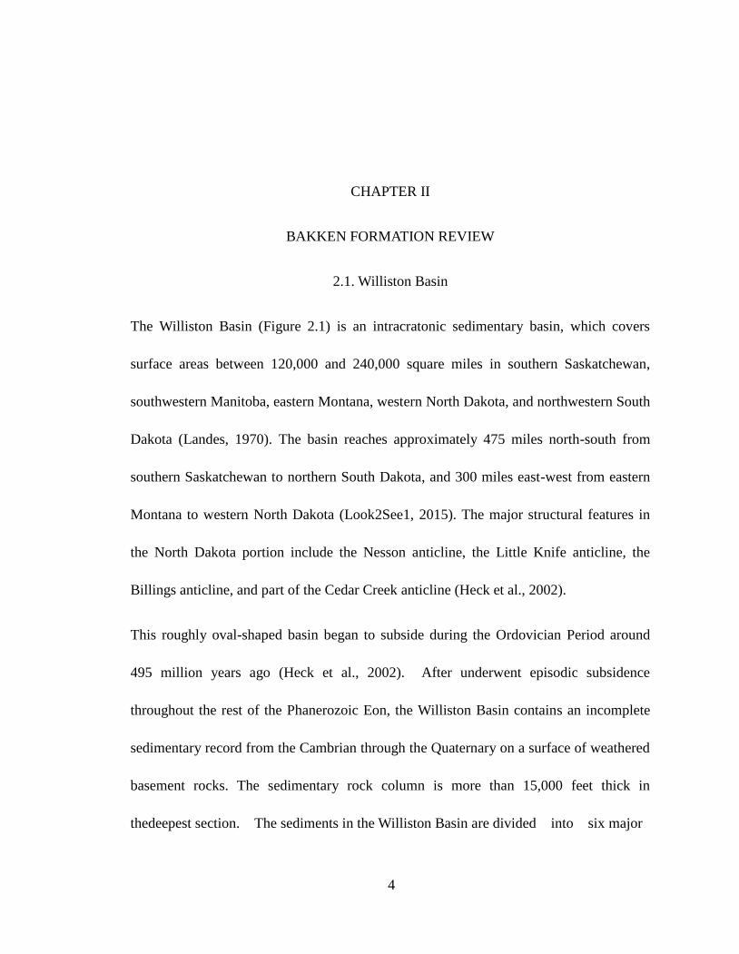
The Williston Basin (Figure 2.1) is an intracratonic sedimentary basin, which covers
surface areas between 120,000 and 240,000 square miles in southern Saskatchewan,
southwestern Manitoba, eastern Montana, western North Dakota, and northwestern South
Dakota (Landes, 1970). The basin reaches approximately 475 miles north-south from
southern Saskatchewan to northern South Dakota, and 300 miles east-west from eastern
Montana to western North Dakota (Look2See1, 2015). The major structural features in
the North Dakota portion include the Nesson anticline, the Little Knife anticline, the
Billings anticline, and part of the Cedar Creek anticline (Heck et al., 2002).
This roughly oval-shaped basin began to subside during the Ordovician Period around
495 million years ago (Heck et al., 2002). After underwent episodic subsidence
throughout the rest of the Phanerozoic Eon, the Williston Basin contains an incomplete
sedimentary record from the Cambrian through the Quaternary on a surface of weathered
basement rocks. The sedimentary rock column is more than 15,000 feet thick in
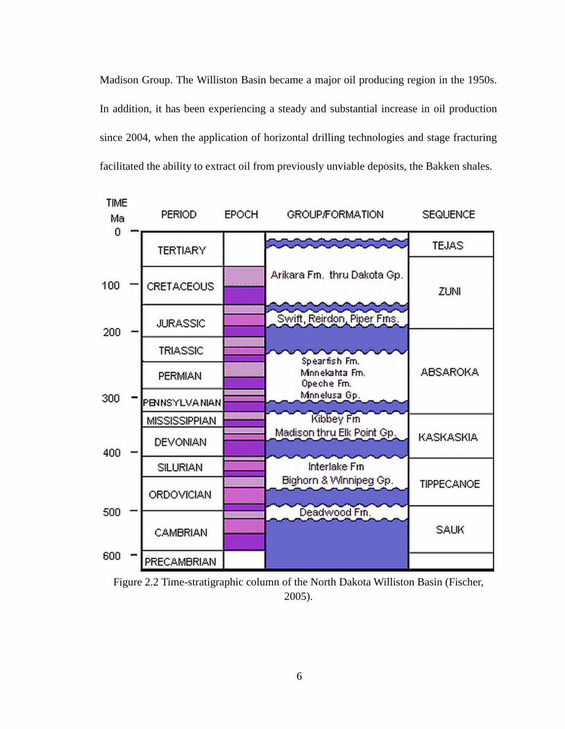
thedeepest section. The sediments in the Williston Basin are divided into six major

5
sequences based on the transgression and regression events, and each sequence contains
couple formations (Figure 2.2). These sequences are, in ascending order, the Sauk,
Tippecanoe, Kaskaskia, Absaroka, Zuni, and Tejas (Sloss, 1963).
Figure 2.1 Williston Basin and its major structures (Heck et al, 2002).
In the Williston Basin, the most produced hydrocarbons are from carbonate reservoirs
from the Ordovician through the Mississippian. Although several companies explored for
oil starting in 1917, the boom in leasing and drilling activities in the Williston Basin is
led by the first commercial oil discovery well, Amerada’s Clarence Iverson No.1, which
struck commercial quantities of oil south of Tioga, ND at a depth greater than 11,000 feet
below the surface in 1951. This discovery well was completed in the Silurian Interlake
Formation but subsequent development on the anticline focused on the Mississippian
6
Madison Group. The Williston Basin became a major oil producing region in the 1950s.
In addition, it has been experiencing a steady and substantial increase in oil production
since 2004, when the application of horizontal drilling technologies and stage fracturing
facilitated the ability to extract oil from previously unviable deposits, the Bakken shales.
Figure 2.2 Time-stratigraphic column of the North Dakota Williston Basin (Fischer,
2005).

7
2.2. Bakken Formation
The Bakken Formation, a large subsurface formation within the Williston Basin (Figure
2.3), is known for its rich petroleum deposits. Currently, the Bakken Formation is
considered the main reservoir and source of a huge portion of the oil generated and
produced in the Williston Basin.
Figure 2.3 Map of the Bakken Formation (Dukes, 2013)
2.2.1. Geology of Bakken Formation
The Bakken Formation formed during the late Devonian and early Mississippian age,
which is included in the Kaskaskia Sequence (Hester and Schmoker 1985). The Bakken
Formation underlies the Mississippian Lodgepole Formation and overlies the Devonian

8
Three Forks Formation conformably in the Williston Basin, except that the
unconformable contact exists at the flanks of the basin between the Bakken Formation
and the Three Forks Formation.
With an offshore marine environment (LeFever, 1991), the Bakken Formation consists of
three members: the upper shale, the lithologically variable middle member, and the lower
shale. The thin and naturally fractured upper and lower shales have rich organic content,
which are considered both a source and reservoir. In North Dakota, the middle member
of the Bakken Formation is mainly gray interbedded siltstones and sandstones with a
maximum thickness of 85 feet occurring at depths of approximately 9,500 to 10,000 feet
(Heck et al., 2002).
2.2.2. Production History of Bakken Formation
The Bakken Formation is very thin compared to other oil producing horizons, but it has
recently attracted much attention because the extremely high hydrocarbon content of the
Bakken Formation has placed it among the richest hydrocarbon source rocks in the world.
The estimate of original oil in place (OOIP) for the Bakken Formation ranges from 200
to more than 400 billion barrels (Price, 2000). This unconventional reserve in the Bakken
Formation becomes increasingly important when the growth rate of demand outpaces the
one of new reserves on oil and gas.

9
Figure 2.4 Development history of the Bakken in Williston Basin (Nordeng, 2010).
During the period from 1953 to 1987, vertical wells were drilled to recover the crude oil
from the Bakken Formation (Figure 2.4). The wells that encountered natural fractures
were successful, but those wells displayed high production at the beginning and soon
dropped rapidly to a steady, low level production rate. In the beginning of 1990s, the
horizontal drilling was extensively practiced in the Bakken Formation (Carlisle et al.,
1996). These wells performed quite well in the “Bakken Fairway” area in North Dakota.
Due to the high investment, the horizontal wells are usually drilled for two purposes:
increasing the drainage area in thin layers, and/or connecting more fractures in naturally
fractured reservoirs (Economides and Boney, 2000). The success of horizontal well

10
depends on two factors: (1) vertical permeability and (2) wellbore orientation with
respect to natural fractures (Karcher et al., 1986; Mukherjee and Economides, 1991;
Hudson and Matson, 1992). Using horizontal drilling has improved the performance to a
certain degree, especially with the successful production of oil from the upper shale of
the Bakken Formation.
The horizontal well also encountered new challenges: the borehole instability and the
wellbore interference. The large investment and high risk in drilling horizontal well in
the Bakken Formation kept the exploration and production activities at a low level until
2000 when new well construction technique was developed in Richland County, Montana
(Lantz et al., 2007), which later extended to western North Dakota. This new technique
combines horizontal drilling with hydraulic fracturing. Since 2006 a significant amount
of oil has been successfully produced from the Bakken Formation.

11
CHAPTER III
METHODOLOGY
3.1. Sample Selection
As shown in Figure 3.1, the Bakken Formation in U.S. was divided into five continuous
assessment units (AU): (1) Elm Coulee-Billings Nose AU, (2) Central Basin-Poplar
Dome AU, (3) Nesson-Little Knife Structural AU, (4) Eastern Expulsion Threshold AU,
and (5) Northwest Expulsion Threshold AU. The boundaries of these assessment units
are consistent with the major structures in the area, and support the aforementioned
geological heterogeneity.
The Bakken core samples were chosen as the specimens from eight wells in the five AU.
These wells are chosen based on the thickness of the Bakken Formation and the
condition of the core. The corresponding North Dakota Industrial Commission (NDIC)
file number, the map number, and the tops of the members of the Bakken Formation are
listed in Table 3.1 for each well.

12
Figure 3.1 Five continuous assessment units of the Bakken Formation (Modified from
Pollastro et al., 2008).
Table 3.1 Wells providing core samples for test in this study
Map
Number
NDIC File
Number Assessment Unit
Top of Formation (ft)
Upper
Bakken
Middle
Bakken
Lower
Bakken
2 11617 Nesson-Little Knife Structural AU 10310 10330 10380
13 15923 Central Basin-Poplar Dome AU 10985 11005 11050
18 16089 Northwest Expulsion Threshold AU 8595 8610 8675
20 16174 Elm Coulee-Billings Nose AU 10673 10683 10712
70 16862 Eastern Expulsion Threshold AU 8803 8820 8850
72 16985 Central Basin-Poplar Dome AU 10486 10510 10550
86 17450 Northwest Expulsion Threshold AU 7300 7355 7415
96 16771 Nesson-Little Knife Structural AU 10288 10307 10378

13
3.2. Sample Prepare and Main Equipment
Our literature review indicates that numbers of core analysis on shale are limited due to
the difficulty in preparing shale plug from drilling cores. The brittle nature of shale
makes the successful rate of preparing plug very lower from drilling core. Usually the
successful rate ranges from 0 to 10%. To overcome the sampling difficulty, the freezing
sample method is used in preparing the plug for core analysis. The core was pre-cooled at
low temperature for several days, and drilled with the equipment show in Figure 3.2. The
core plugs were prepared into cylindrical pieces of one inch in diameter and two inches
in length. Two hundred and forty specimens in total were used in the test, of which 42
from Upper Bakken, 140 from Middle Bakken, and 58 from Lower Bakken.
Figure 3.2 Core plug sampling system used in this study
First, the dry bulk density of the specimens was measured after the specimens were oven

14
dried and weighed; then the non-destructive properties, porosity, permeability, velocity,
elastic moduli, compressibility, and Biot’s coefficient, were measured step by step; at the
end the destructive properties (compressive strength) was measured.
Figure 3.3 AutoLab-1500 used in this study.
The main equipment that is used to perform our experiments is AutoLab-1500, which is
made by New England Research Inc. AutoLab-1500 is a complete laboratory system with
three integrated components: 1). a pressure vessel and four associated pressure
intensifiers to generate pressures on the test sample; 2). an electronics console that
interfaces with the mechanical system to precisely control the state of pressure and to
condition and amplify signals from the transducers and devices measuring force, pressure,

15
displacement, strain, and temperature; and 3). a data acquisition system which generates
reference signals to control the equipment, to acquire data, and to process the data
collected on the experiment.
AutoLab-1500 supports a comprehensive suite of physical rock properties measurements
as a function of the state of stress and temperature (AutLab-1500, 2009). Figure 3.3 is an
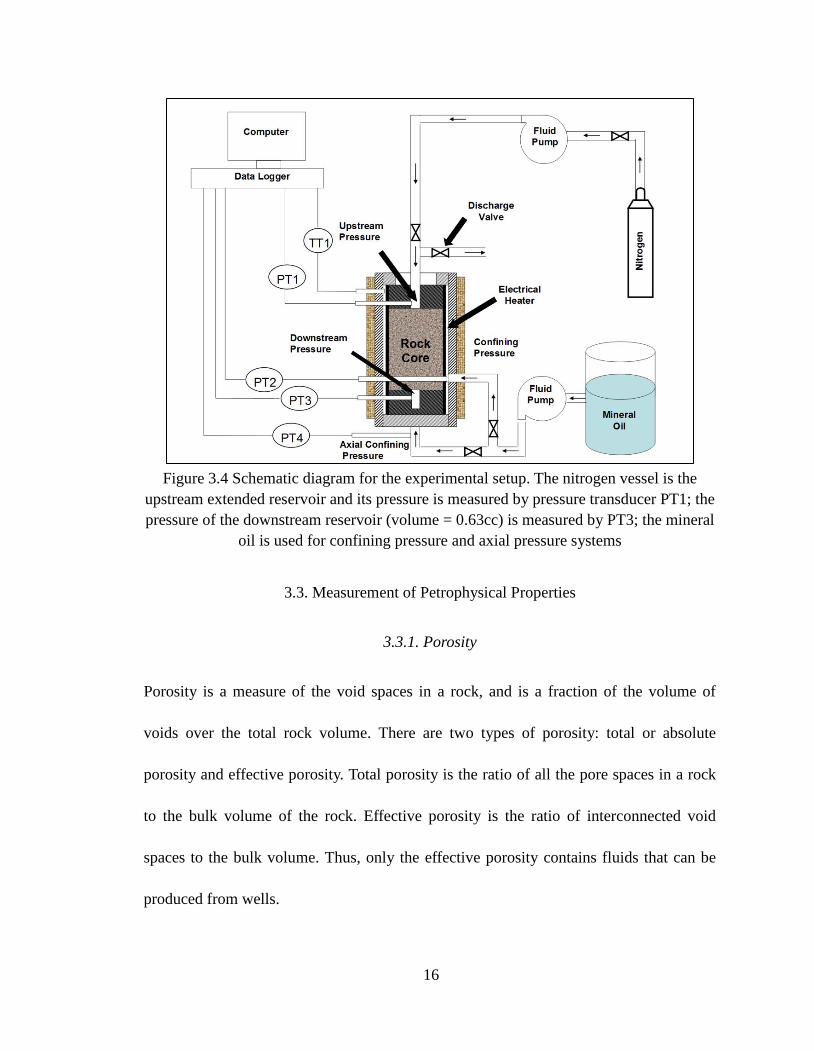
image of AutLab-1500 used in this study. Figure 3.4 presents a conceptual diagram of the
test facility. One temperature transducer (TT1) is used to measure the temperature. Four
pressure transducers (PT1, PT2, PT3, and PT4) are used to measure the upstream
reservoir pressure, the confining pressure at the flank of the core, the downstream
reservoir pressure, and the axial pressure at the ends of the core, respectively.
AutLab-1500 conveniently runs most standard rock mechanics test regimens, such as
hydrostatic compression, pure shear, unconfined compression, confined compression,
creep, and uniaxial strain. Each of these tests can be performed at pore pressures and
temperatures representative of reservoir conditions. The system can also measure rock
permeability, and sonic velocity.
16
Figure 3.4 Schematic diagram for the experimental setup. The nitrogen vessel is the
upstream extended reservoir and its pressure is measured by pressure transducer PT1; the
pressure of the downstream reservoir (volume = 0.63cc) is measured by PT3; the mineral
oil is used for confining pressure and axial pressure systems
3.3. Measurement of Petrophysical Properties
3.3.1. Porosity
Porosity is a measure of the void spaces in a rock, and is a fraction of the volume of
voids over the total rock volume. There are two types of porosity: total or absolute
porosity and effective porosity. Total porosity is the ratio of all the pore spaces in a rock
to the bulk volume of the rock. Effective porosity is the ratio of interconnected void
spaces to the bulk volume. Thus, only the effective porosity contains fluids that can be
produced from wells.

17
For oil and gas reservoirs, porosity provides the space to store the fluid subsurface.
Porosity measurements were conducted to evaluate the storage ability of Bakken
Formation. In this study, the measured porosity is effective porosity.
Equipment
The porosity of core plug was measured by gas compression method which employs real
gas law. Helium is used as the test fluid because it has small molecular size and inertial
property, and it does not adsorb on the rock surface. The porosimeter apparatus is shown
schematically in Figure 3.5. This system consists of gas source, three pressure gauges,
and two chambers. The core is put in Chamber 2.
Figure 3.5 Schematic diagram of porosimeter apparatus
Measurement Principle
The measurement principle is based on real gas law. Followings are the derivation of
governing equation to measure the core porosity.
Firstly, the sum of the volume of Chamber 1 and pipeline volume between Gas Inlet

18
Valve and Gas Outlet Valve is denoted as Volume 1, V1.
1 chamber1 pipeline between Gas Inlet Valve and Gas Inlet ValveV V V (3.1)
Similarly, the sum of the volume of Chamber 2 (without core) and pipeline volume
between Gas Outlet Valve and Gas Vent Valve is denoted as Volume 2, V2.
2 chamber 2 pipeline between Gas Outlet Valve and Gas Vent ValveV V V (3.2)
The bulk volume of core is denoted as Vbulk, core, which is calculated by
2
, core4
bulk core coreV D L
(3.3)
Initially the pressure in Chamber 1 is p1 and pressure in Chamber 2 is p2, where p1> p2.
Then Gas Outlet Valve is open to allow gas flow from Chamber 1 to Chamber 2 and
reach equilibrium. The equilibrium pressure, p3, is recorded. According to real gas law
we have
1 1 1 1 1pV z n RT (3.4)
2 2 , 2 2 21bulk corep V V z n RT (3.5)
3 2 , 1 3 1 2 31bulk corep V V V z n n RT (3.6)
The temperature is kept constant and pressure is changed in a narrow range. Therefore
we have
1 2 3z z z (3.7)
Equations (3.4), (3.5), and (3.6) can be simplified into
19
1 1 1 1 1pV z n RT (3.8)
2 2 , 1 2 11bulk corep V V z n RT (3.9)
3 2 , 1 1 1 2 11bulk corep V V V z n n RT (3.10)
Summing Equations (3.8) and (3.9) we obtain
2 2 , 1 1 1 1 2 11bulk corep V V pV z n n RT (3.11)
Comparing the right-hand-sides of Equations (3.10) and (3.11) gives us
2 2 , 1 1 3 2 , 11 1bulk core bulk corep V V pV p V V V (3.12)
Rearranging Equation (3.12) yields
1 3 12
, 3 2 ,
1bulk core bulk core
p p VV
V p p V
(3.13)
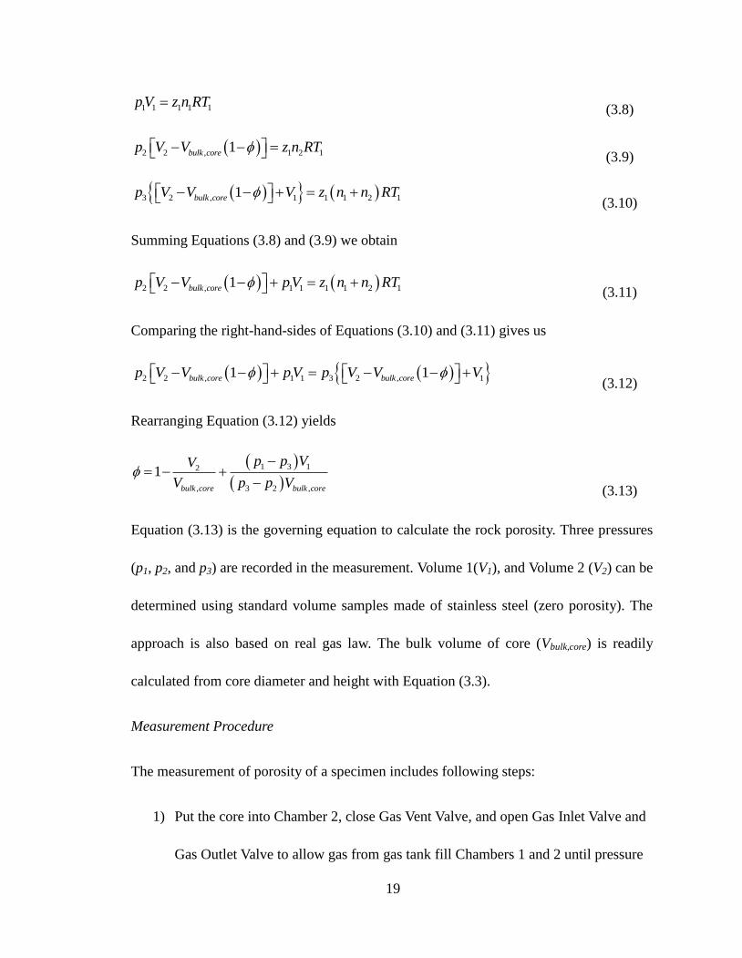
Equation (3.13) is the governing equation to calculate the rock porosity. Three pressures
(p1, p2, and p3) are recorded in the measurement. Volume 1(V1), and Volume 2 (V2) can be
determined using standard volume samples made of stainless steel (zero porosity). The
approach is also based on real gas law. The bulk volume of core (Vbulk,core) is readily
calculated from core diameter and height with Equation (3.3).
Measurement Procedure
The measurement of porosity of a specimen includes following steps:
1) Put the core into Chamber 2, close Gas Vent Valve, and open Gas Inlet Valve and
Gas Outlet Valve to allow gas from gas tank fill Chambers 1 and 2 until pressure
20
reaches 100 psig.
2) Open Gas Vent Valve and allow gas from gas tank purge Chambers 1 and 2, Wait
for 10 to 20 minutes until the purity of gas in Chambers 1 and 2 is high enough.
3) Close Gas Vent Valve, Gas Inlet Valve, and Gas Outlet Valve, record the pressure
of Chamber 2, p2.
4) Keep Gas Vent Valve and Gas Outlet Valve close, Open Gas Inlet Valve and allow
gas from gas tank fill Chamber 1 until its pressure reaches target pressure, close
Gas Inlet Valve and record the pressure of Chamber 1, p1.
5) Open Gas Outlet Valve to allow gas flow from Chamber 1 to Chamber 2 (because
p1 > p2), wait until pressure reaches equilibrium, or pressure at Pressure Gauge 3
equates pressure at Pressure Gauge 2, record equilibrium pressure, p3.
6) Now we finish the porosity measurement of specimen. Porosity can be calculated
by Equation (3.13).
3.3.2. Permeability
Permeability is a property of a porous medium and is an indicator of its ability to allow
fluids flow through its inter-connected pores. Permeability is an inherent characteristic of
the porous media only. It depends on the effective porosity of the porous media (Triad,
2004).
The fundamental SI unit of permeability is m2, but the Darcy (D), named after French
engineer Henry Darcy, is a practical unit for permeability. One Darcy is defined as

21
follows: a permeability of one Darcy will allow a flow of 1 cm3/s of fluid of 1 centipoise
(cp) viscosity through an area of 1 cm2 under a pressure gradient of 1 atm/cm. One Darcy
equals 0.986923 × 10⁻¹²
m2. In the oil and gas industry, a smaller unit of permeability,
milli-Darcy (mD), is used more commonly because the permeability for most rocks is
less than one Darcy, and for the low permeability rocks, the use of micro-Darcy (μD) or
nano-Darcy (nD) is common.
The range of the permeability of the petroleum reservoir rocks may be from 0.1 to 1,000
mD. One rock is considered to be tight when its permeability is below 1 mD (Triad,
2004). However, this criterion has been lowered to values of 0.1mD (Law & Spencer,
1993) due to the application of the new stimulation techniques to increase oil and gas
production.
Tight rocks have been extensively studied for a wide range of applications that include
CO2 geological storage, deep geological disposal of high-level, long-lived nuclear wastes,
and production of oil and gas from unconventional reservoirs. In the recent years, the
increasing demands for oil and gas have stimulated the explorations and productions of
petroleum from low permeability formations, such as Bakken shale. More realistic fluid
flow simulation to model the process of producing the hydrocarbons in Bakken
Formation requires more accurate measurements of permeability. Also it is urgent to
investigate the low permeability of the Bakken Formation in order to gain better
understanding of the process of well producing hydrocarbons from it.

22
Based on experimental work from Darcy (1856), many methods have been presented to
improve the accuracy and efficiency of measurement. These methods, based on flow
regime, can be classified into two categories: steady-state flow methods and
unsteady-state flow methods. Steady-state flow methods measure permeability under
steady-state conditions. Aside from low flow rates across the core plug being difficult to
measure and control, these tests are quite time consuming. In this case, unsteady state
flow is applied to estimate permeability. Brace et al. (1968) introduced a transient flow
method to measure the permeability of Westerly granite. From this, many unsteady-state
methods have been proposed to measure the permeability of tight rocks. Most of these
methods fall into three categories: the pulse decay method, the Gas Research Institute
(GRI) method, and the oscillating pulse method.
For the pulse-decay method, the sample has both an upstream reservoir and a
downstream reservoir. A pressure pulse, which is applied at the upstream reservoir, will
decay over time. The permeability is estimated by analyzing the decay characteristics of
the pressure pulse (Brace et al., 1968). Dicker and Smits (1988) improved the pressure
pulse-decay method by showing a general solution of the differential equation which
describes the pressure decay curve. Based on this solution, they theoretically pointed out
that fast and accurate measurements are possible when the volumes of the upstream and
downstream reservoirs in the equipment are equal to the pore volume of the sample.
Jones (1997) pointed out that the initial pressure equilibration step is the most
23
time-consuming part of the pulse-decay technique. To avoid the equilibrium state, Jones’
method utilizes a smooth pressure gradient, which requires smaller upstream and
downstream reservoirs. To account for adsorption during pulse-decay measurement, Cui
et al. (2009) presented their method which can describe gas transport in low permeability
reservoir more reliably and accurately. Metwally (2011) proposed another pulse-decay
method by keeping the upstream reservoir pressure constant leading to an infinitely large
volume of the upstream reservoir, so that the ratio of upstream reservoir volume to
downstream reservoir volume is infinite. Thus, the solution of the pulse-decay
measurements can be simplified.
The GRI method differs from the pulse-decay method in that the measurement is carried
out on crushed rock samples; a pressure pulse is applies on unconfined crushed rock
particles. Permeability is then obtained through the analysis of the pressure decay over
time. Cui et al. (2009) developed a late-time method utilizing data from either
pulse-decay or GRI experiment to determine the permeability. The GRI method has the
advantage of a shorter experimental time as compared with other methods. Unfortunately,
permeability measured from crushed samples can differ by 2 to 3 orders of magnitude
among different commercial laboratories (Passey et al., 2010 and Tinni et al., 2012).
Another limitation of this method is that the microcracks in the crushed particles
essentially violate the GRI assumptions. This leads to an overestimate of permeability
(Tinni et al., 2012). To improve the accuracy and consistency of the GRI method, Sinha

24
(2012) developed cylindrical calibration standards based on Darcy’s law to calibrate the
low permeability measurement apparatus. The GRI method is not used in this study
because of large permeability differences between crushed and intact samples.
The oscillating pulse method estimates rock permeability by interpreting amplitude
attenuation and phase retardation in the sinusoidal oscillation of the pore pressure as a
pressure pulse propagates through a sample. At the beginning of the experiment, the
sample pore pressure, the upstream reservoir pressure, and the downstream reservoir
pressure are stabilized. Then a pressure wave is generated in the upstream reservoir and
propagates through a core plug. The permeability can be obtained by using the
information of the amplitude attenuation and phase shift between the upstream reservoir
pressure wave and the derived downstream reservoir pressure wave at the downstream
side of the sample. Although this method can measure the permeability in a relatively
short time without destroying the sample, as the GRI method does, the accuracy of
permeability obtained from this method relies on the signal-to-noise ratio and data
analysis techniques (Kranz et al., 1990).
Normally, permeabilities measured by the different methods are not in good agreement.
Bertoncello (2013) concluded that the steady-state method with critical fluid provides
much more consistent and acceptable results after comparing permeability measurements
performed at several commercial and research laboratories using four different
techniques. However, Bertoncello (2013) did not mention the time of measurement for

25
each method. In fact, the measurement of tight rock permeability, such as in Bakken
samples, is time consuming and expensive due to their low permeability. In addition, the
results given by Lab_1 from transient methods are consistent and acceptable, and Lab_1
is the only laboratory which provides different methods.
We introduced a testing process to measure the permeability of tight rocks with three
different methods under the same procedure. These methods are the oscillating pulse
method, the downstream pressure build-up method, and the radius-of-investigation
method. In this way, not only the comparability of the results from these three methods
increased, but the difference among the results is also useful for indicating the
heterogeneity and/or microcracks of the rock.
Method 1: Oscillating Pulse Measurement Method
Figure 3.6 Illustration of the effect of the upstream input oscillation frequency on the
resultant downstream amplitude and phase shift of the oscillating pulse method

26
Figure 3.6 indicates the theory of the aforementioned oscillating pulse method (Kranz et
al., 1990). A pressure oscillation with fixed-amplitude and fixed-frequency in the
upstream reservoir results in a reduced amplitude and phase-shifted pressure oscillation
in the downstream reservoir after diffusing through the core sample. The amplitude ratio
and phase shift provide information about the hydraulic properties of the rock. Based on
these pressure responses, an analytical solution for permeability can be calculated from
either the amplitude ratio or the phase shift. The relationship between the upstream and
downstream perturbations is a function of the length, cross-sectional area, permeability,
specific storage of the sample, the viscosity of the fluid, and the compressibility of the
fluid. Appendix A provides the derivation of equations for this method given by Kranz et
al. (1990). However, a strong dependence on the ratio of permeability to specific-storage
creates a situation where an error in the determination of one parameter (i.e. specific
storage) will lead to an error in the determination of the other (i.e. permeability).
Derivation of Diffusivity Equation
The estimations of permeability by the downstream pressure build-up method and the
radius-of-investigation method require the solution of the diffusivity equation for the
Darcy flow through the core sample. To derive the diffusivity equation, the following
assumptions are made: 1) the core is homogeneous, 2) the properties of the rock are
constant, 3) the flow in the cylindrical core is laminar, and 4) the flow in the core is
isothermal. Because the permeability of tight rock is low, nitrogen gas is used as the test

27
fluid in our experiment. The gas flows from the left-side of the core, through the core,
and out of the right-side of the core as shown in Figure 3.7.
Figure 3.7 Schematic diagram depicting how gas flows through a core
Considering a control volume (from x to x+Δx), which is the volume that the gas flows in
from x and out at x+Δx during a certain time period Δt, and combining the mass
conservation, Darcy’s law, real gas law, and the gas pseudo-pressure concept
(Al-Hussainy, 1966), a diffusivity equation for linear gas flow is stated as:
2
2m( ) m( )
x
tcp p
k t
(3.14)
where m(p) is the gas pseudo-pressure, which is expressed as
b
p
p
2m( ) dp
μz
pp
(3.15)
Method 2: Downstream Pressure Build-up Measurement Method
In the downstream pressure build-up method, the upstream reservoir pressure is kept
constant throughout the entire test and the pressure build-up is observed in the
Core
△p
x+△x
p+△p
x △x
p
K D
P2
x=L x=0
P1
Control
Volume
qg
A
L

28
downstream reservoir when the gas flows through the core plug into it.
To calculate the permeability from the build-up curve of the measured downstream
reservoir pressure, the solution to the diffusivity Equation (3.14) needs to be known.
Permeability is then estimated through Equation (B.14). The derivation of equations for
this method is in Appendix B.
Method 3: Radius-of-Investigation Measurement Method
Based on the Radius-of-Investigation Concept (Lee, 1982), a new method was proposed
to measure core permeability. When doing the permeability test using the downstream
pressure build-up method, it was observed that the downstream reservoir pressure did not
increase immediately when the upstream reservoir was connected with the core plug.
The lower the permeability, the longer the delay time was observed. The time that a
pressure disturbance propagates through a core sample is a function of the permeability
of the rock. Therefore, the low to extremely low permeability of Bakken samples can be
calculated by measuring the delaying time, which is the time that the pressure
disturbance propagates from the upstream end of the core plug to the downstream end of
the core plug.
The pressure disturbance concept is applied here to estimate the propagation of pressure
in the core plug. First, a pressure disturbance was introduced by increasing the
upstream reservoir pressure or decreasing the downstream reservoir pressure
instantaneously; then the time (tm) at which the disturbance at location x reaches its

29
maximum was determined. With measured tm and given core geometry, the permeability
can be obtained using Equation (C.7). The derivation of equations for this method is in
Appendix C.
Measurement Procedure
First, the cylindrical Bakken core plug was covered with copper sheeting in order to both
form a gas-tight seal on the cylindrical wall of the sample and to apply radial confining
pressure. Then the core plug was mounted in a sample holder with flexible rubber sleeves
at both ends of the plug (Figure 3.7). Finally, the sample holder was put into a vessel
flooded with mineral oil, in which the sample could be hydrostatically compressed by
hydraulically applying force to the plug. To minimize the volume of the downstream
reservoir, a small pocket was implemented inside the downstream end-cap (Figures 3.8).
The volume of downstream reservoir was 0.63 cc.
Figure 3.8 Core covered with copper sheeting, and assembled on End Caps for a low
permeability test system
The equipment used to perform the experiments is AutLab-1500. The determination of
Gas in
Downstream Reservoir inside
30
the permeability is a three-step process for all of these three methods, namely installing
the core plug into the AutLab-1500, running the test, and analyzing the resultant data.
1) Installing the core plug into the AutLab-1500
First, the sample is placed into the vessel; then the vessel is filled with mineral oil and
the confining pressure is increased to the desired level (pc). The valve between the core
plug and the upstream reservoir is closed. Dry nitrogen is used to fill the upstream
reservoir, and the upstream reservoir pressure is increased to the desired level (p1). The
downstream reservoir is at atmospheric pressure. Notice that the confining pressure must
be greater than the upstream reservoir pressure.
2) Running the test
The start time is recorded when the valve between the core plug and the upstream
reservoir is opened. During the entire test, the upstream reservoir and confining pressures
are constant. The pressures are monitored and recorded at both the upstream and
downstream ends of the sample.
Figure 3.9 shows the change of downstream reservoir pressure during the test. A constant
pressure is applied at the upstream end of the core plug, and the pressure at the
downstream end of the core plug is built up. For the radius-of-investigation method, the
test ends when the downstream reservoir pressure starts to increase, which is at point “B”.
For the downstream pressure build-up method, the test ends when the downstream
reservoir pressure is equal to the upstream reservoir pressure, which is at point “A”. For

31
the oscillating pulse method, the test ends at the point “C”.
Figure 3.9 Changes of the upstream and downstream pressure during one experiment for
Core #1.
Point “A” marks the time at which the downstream pressure build-up method stop,
point “B” marks the time at which the radius-of-the investigation method stop,
and point “C” marks the time at which the oscillating pulse method stop

32
3) Analyzing the resultant data
For the radius-of-investigation method, after finding the time of point “B”, the
permeability can be obtained using Equation (C.7) or (C.8). To better determine point
“B”, the section from constant downstream pressure to downstream pressure build-up is
amplified.
The beginning point of the increasing in downstream pressure is selected as point “B”,
and the section “BA” shows the pressure change in the downstream reservoir as a
function of time (Figure 3.9). To obtain the permeability using the downstream pressure
build-up method, first the pressure difference is calculated using a logarithm scale form
equation )()0(ln)(ln
2
2
2
1 tpptp ; then from the plot (Figure B.1), we obtain the
slope s; finally, Equation (B.16) is used to obtain the permeability of the rock (see
Appendix B).
For the oscillating pulse method, the AutLab-1500 system directly gives the permeability.
3.4. Measurement of Geomechanical Properties
3.4.1. Elastic Moduli
Rocks will behave a linear elastic material approximately if the stresses they are
subjected to are considerably lower than their ultimate strengths. The basic elastic
constants, such as Young’s modulus, Poisson’s ratio, shear modulus, bulk modulus, and
Lame constant, are based on this linear elasticity theory, For homogeneous isotropic

33
linear materials, given any two elastic moduli, any other elastic moduli can be calculated
with conversion formulas (Zhou, 2011). In our study, we measured two independent
elastic constants, Young’s modulus and Poisson’s ratio; the other elasticity parameters
can be derived from these two parameters.
Static Young’s Modulus and Poisson’s Ratio
Young’s modulus, also known as the tensile modulus or elastic modulus, is a measure of
the stiffness of an elastic material and is a quantity used to characterize materials. It is
defined as the ratio of the stress along an axis to the strain along that axis in the range of
stress in which Hooke's law holds. When Young's modulus is calculated from
deformational experiment directly by dividing the tensile stress by the tensile strain in the
elastic (linear) portion of the stress-strain curve (Figure 3.10), it is called static Young’s
modulus.
staticE
(3.16)
where Estatic is the static Young’s modulus, σ is the axial stress exerted on specimen, and
ε is the strain of specimen in axial direction.
Poisson's ratio, , named after Siméon Poisson, is the negative ratio of transverse to axial
strain. When a material is compressed in one direction, it usually tends to expand in the
other two directions perpendicular to the direction of compression (Figure 3.11). This
phenomenon is called the Poisson effect. The Poisson ratio is the ratio of the fraction of
34
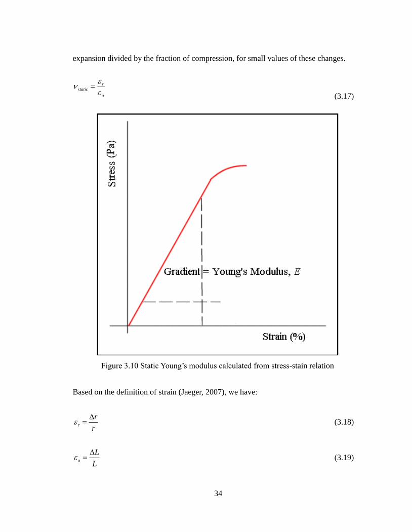
expansion divided by the fraction of compression, for small values of these changes.
rstatic
a
(3.17)
Figure 3.10 Static Young’s modulus calculated from stress-stain relation
Based on the definition of strain (Jaeger, 2007), we have:
r
r
r
(3.18)
a
L
L
(3.19)

35
εr is the strain of specimen in radial direction, and εa is the strain of specimen in axial
direction.
If the material is stretched, it usually tends to contract in the directions transverse to the
direction of stretching. The Poisson’s ratio will be the ratio of relative contraction to
relative stretching, and will have the same value as above. Due to the requirement that
Young's modulus, the shear modulus and bulk modulus have positive values, Poisson's
ratio can vary from initially 0 to about 0.5. Generally, "stiffer" materials will have lower
Poisson's ratios than "softer" materials. If Poisson’s ratios are larger than 0.5, it implies
that the material was stressed to cracking, or caused by experimental error, etc.
Figure 3.11 Poisson’s ratio from a deformed cylinder-shape specimen (Poisson’s Ratio,
2007)
36
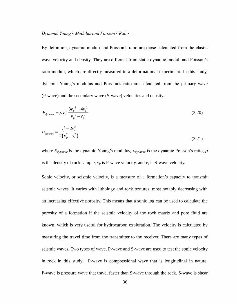
Dynamic Young’s Modulus and Poisson’s Ratio
By definition, dynamic moduli and Poisson’s ratio are those calculated from the elastic
wave velocity and density. They are different from static dynamic moduli and Poisson’s
ratio moduli, which are directly measured in a deformational experiment. In this study,
dynamic Young’s modulus and Poisson’s ratio are calculated from the primary wave
(P-wave) and the secondary wave (S-wave) velocities and density.
2 2
2
2 2
3 4p s
dynamic s
p s
v vE v
v v
(3.20)
2 2
2 2
2
2
p s
dynamic
p s
v v
v v
(3.21)
where Edynamic is the dynamic Young’s modulus, dynamic is the dynamic Poisson’s ratio,
is the density of rock sample, vp is P-wave velocity, and vs is S-wave velocity.
Sonic velocity, or seismic velocity, is a measure of a formation’s capacity to transmit
seismic waves. It varies with lithology and rock textures, most notably decreasing with
an increasing effective porosity. This means that a sonic log can be used to calculate the
porosity of a formation if the seismic velocity of the rock matrix and pore fluid are
known, which is very useful for hydrocarbon exploration. The velocity is calculated by
measuring the travel time from the transmitter to the receiver. There are many types of
seismic waves. Two types of wave, P-wave and S-wave are used to test the sonic velocity
in rock in this study. P-wave is compressional wave that is longitudinal in nature.
P-wave is pressure wave that travel faster than S-wave through the rock. S-wave is shear

37
wave that is transverse in nature. P-wave can travel through any materials. S-wave can
travel only through solids, as fluids (liquids and gases) do not support shear stresses.
S-wave is slower than P- wave.
Measurement Procedure
AutLab-1500 is used to perform our experiments. Static dynamic moduli and Poisson’s
ratio moduli are directly measured in a deformational experiment. The strains in the axial
and radial directions of core plug are monitored by strain gages (Figure 3.12). The
compressional stresses in the axial and radial directions are also recorded. Figure 3.13
shows an example of stress and strain in a non-destructive strength test in this study.
Figure 3.12 Image of sample with strain gages
Dynamic Young’s modulus and Poisson’s ratio are calculated from the results of sonic
velocity test in the AutLab-1500, in which the ultrasonic signal is excited and captured
by a pulser-receiver. Once the experiment has been completed, the data is edited and
plotted.
The first step is to display the waveforms and pick the times of first arrival for each wave
type: compressional or polarized shear wave. After the times of first arrival of P-wave
(Figure 3.14), first S-wave (Figure 3.15), and second S-wave (Figure 3.16) are selected,

38
the velocities of P-wave and S-wave are calculated with the length of sample and the
time. An example of the compression and shear wave velocities of core plug are shown in
Figure 3.17.
Figure 3.13 An example of stress and strain in a triaxial test
(K: Bulk modulus, G: Shear modulus, E: Young’s modulus, n: Poisson’s ratio, P: Constrained modulus.)

39
Figure 3.14 Waveform for P arrivals

40
Figure 3.15 Waveform for S1 arrivals

41
Figure 3.16 Waveform for S2 arrivals

42
Figure 3.17 Dynamic properties calculated from sonic velocity
Because we want to compare the Young’s modulus and Poisson’s ratio from both tests,
the measurement procedure is design as below.
First cover the sample with a copper foil and attach strain gages on the wall of the sample
to monitor the deformation of the sample during the experiment. Then insert the sample
between the velocity transducer assemblies, which are pulse-receiver embedded in the

43
two end-caps at both ends of the sample, to measure the velocities of P- and S-waves.
Figure 3.18 shows a core holder with an instrumented Bakken sample that is jacketed and
positioned between velocity transducer assemblies with strain-gauges attached. Finally,
install the core holder into the pressure vessel of the AutoLab-1500.
Figure 3.18 Core holder with an instrumented Bakken sample that is jacketed and
positioned between velocity transducers with strain gages attached
For appropriate comparison, the static and dynamic moduli were determined within the
same situation. The tri-axial compression test was done with four loading cycles. The
Young's modulus was obtained from the cycles except the first cycle to eliminate the
effect of the first loading (Bruno, 1991). The test deformation rate is constant (0.01 mm
per minute), the confining pressure is 30MPa, and the axial stress in the loading is
nominally between 20 and 30 MPa, below failure criteria. The axial and radial strains of
each sample were measured with strain gauges. From Equations (3.16) and (3.17), the
static Young’s modulus and Poisson’s ratio are obtained respectively as shown in Figure

44
3.13.
After the four loading cycles of tri-axial compression test, the velocity test was started to
get the dynamic moduli at the same situation as tri-axial compression test. When P- and
S-waves propagated through the sample, the signals of P- and S-waves were recorded
with the pulse-receiver, and the travel times for each wave type were read from their first
arrivals. Thus the velocities for P- and S-waves were obtained by dividing the sample
length by the travel time. With Equations (3.20) and (3.21) we got the dynamic Young’s
modulus and Poisson’s ratio as shown in Figure 3.17.
The procedure for conducting the experiment is listed as follow:
1) Jacket the sample with copper foil.
2) Attach strain gages to the sample.
3) Secure the sample to the ultrasonic velocity transducer assembly.
4) Insert the transducer assembly with the jacketed sample into the pressure vessel.
5) Fill the pressure vessel with mineral oil.
6) Increase the confining pressure to reservoir level.
7) Increase the differential stress and the confining pressure to the initial value for
the tri-axial compression measurement.
8) Set the loading rate, the range of the axial stress, and the number of loading
cycles for the tri-axial compression test.
9) Start tri-axial compression test, and collect the data.

45
10) End tri-axial compression test.
11) Select P and S waves as the wave types for velocity test.
12) Start velocity test, and store the test data.
13) End velocity test.
14) Calculate static moduli with the data from tri-axial compression test.
15) Calculate dynamic moduli with the data from velocity test, after obtaining the
travel time for P- and S-waves.
3.4.2. Compressibility
Rock compressibility is a measure of the relative volume change of a rock as a response
to a pressure change. It is also called pore compressibility and is expressed in units of
pore volume change per unit pore volume under per unit pressure change (Petrowiki).
Rock compressibility is one of key parameters in designing oil and gas well drilling and
completion, modeling fluids flow in reservoir, and forecasting well production.
There are two methods to obtain rock compressibility. One is direct measurement;
another is indirect measurement. Direct measurement measures compressibility through
uniaxial or triaxial stress experiment. Indirect measurement estimates compressibility
from correlations or other measurements. The importance of rock compressibility is
reflected by numerous investigations attempting to evaluate it accurately.
Carpenter and Spencer (1940) measured compressibility of consolidated oil-bearing
sandstones collected from East Texas oil field at reservoir conditions. Hall (1953)

46
conducted tests to measure limestone and sandstone compressibility in the same manner
as those reported in the Carpenter and Spencer’s study. He developed correlation to
estimate rock compressibility through porosity. Hall found that ignoring rock
compressibility can lead to 30 to 40 percent overestimation of oil in place. Fatt (1958a)
studied the variation of rock compressibility at different pressures. Fatt (1958b) found
that rock compressibility is a function of pressure and cannot be correlated to porosity.
Van der Knaap (1959) proved the nonlinear stress-volume relations of elastic porous
media through theoretical and experimental analysis. Harville and Hawkins (1969)
indicated that rock compressibility of geopressured gas reservoir is higher than that of
normally pressured reservoir. Newman (1973) measured compressibility of 256 samples
taken from consolidated and unconsolidated rocks and compared with Hall’s and van der
Knaap’s studies. Greenwald and Somerton (1981a) measured compressibility of Berea,
Bandera, and Boise sandstones. Comparison of these compressibilities to those available
in the literature indicated qualitative agreement for each of the sandstone types and for
their relative behavior. Greenwald and Somerton (1981b) developed a semi-empirical
model to calculated rock compressibility. Variables required for their model are initial
porosity, clay content, a pore shape factor, a length and aspect ratio of representative
cracks in the matrix grains, the volumetric density of these cracks, and the mineralogical
composition of the sample along with the elastic moduli of the minerals present.
Zimmerman et al. (1986) developed relations to evaluate rock compressibility from
confining and pore pressures. They verified relations through experimental

47
measurements on Berea, Bandera, and Boise sandstones. Poston and Chen (1987)
determined formation compressibility and gas in place in abnormally pressured reservoirs
simultaneously using material balance. Chalaturnyk and Scott (1992) summarized
different geomechanical test procedures and analyzed the results. Khatchikian (1996)
proposed a method using the Gassman equation and reservoir parameters evaluated
through log analysis. Yildiz (1998) predicted rock compressibility using production data.
His method is the same as Poston and Chen’s method. Macini and Mesini (1998)
measured sandstone and carbonate compressibility by both static (deformation tests) and
dynamics (acoustic tests) investigations. Their study showed that compressibility is not
constant, but is a function of reservoir pressure. Marchina et al. (2004) measured
compressibility of reservoir rocks of a heavy oil field under in-situ conditions. Li et al.
(2004) presented a model to calculate rock compressibility using the elastic modulus and
the Poisson's ratio. Suman (2009) estimated rock compressibility under reservoir
conditions at different depleted stages using sonic velocity derived from 4D seismic.
Because direct measurement of rock compressibility is time consuming and cost
expensive. Estimation of rock compressibility from other readily available experimental
data, such as sonic velocity and permeability experiment, is highly demanded.
We developed two methods to determine the rock compressibility using permeability
experimental data. The combination of the proposed method with direct measurement
can be employed to ensure the reliability of the direct measurement and to quantify the
48
uncertainty resulting from lab and human errors, irregular core plug, and/or non-uniform
deformation.
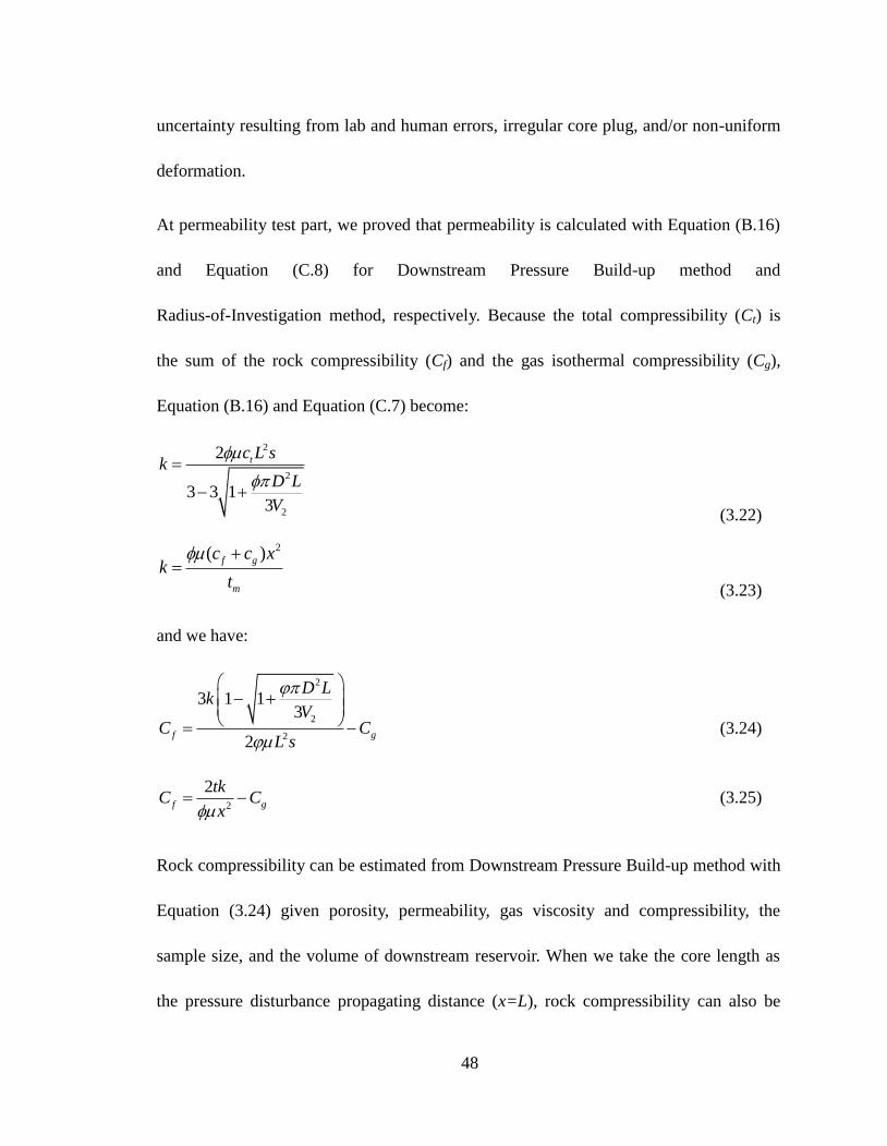
At permeability test part, we proved that permeability is calculated with Equation (B.16)
and Equation (C.8) for Downstream Pressure Build-up method and
Radius-of-Investigation method, respectively. Because the total compressibility (Ct) is
the sum of the rock compressibility (Cf) and the gas isothermal compressibility (Cg),
Equation (B.16) and Equation (C.7) become:
2
2
2
2
3 3 13
tc L sk
D L
V
(3.22)
2( )f g
m
c c xk
t
(3.23)
and we have:
2
2
2
3 1 13
2f g
D Lk
VC C
L s
(3.24)
2
2f g
tkC C
x (3.25)
Rock compressibility can be estimated from Downstream Pressure Build-up method with
Equation (3.24) given porosity, permeability, gas viscosity and compressibility, the
sample size, and the volume of downstream reservoir. When we take the core length as
the pressure disturbance propagating distance (x=L), rock compressibility can also be

49
estimated from Radius-of-Investigation method with Equation (3.25) given porosity,
permeability, gas viscosity and compressibility, and the time for pressure disturbance
travel through the core. The aforementioned derivation of Equation (3.24) or (3.25) uses
gas as test fluid to measure low permeability rocks.
It should be noted that liquid will be used for high permeability rocks. Similarly, liquid
properties can be combined with porosity and permeability, and pressure disturbance
travel time to calculate rock compressibility. Porosity and core length can be measured
readily. Gas viscosity and compressibility can be calculated given gas composition,
pressure, and temperature. Time of pressure disturbance travel through core can be
obtained by recording the time when pressure disturbance is generated and the time it
travels to downstream of the core. Permeability can be obtained by steady-state or
unsteady-state test such as oscillating pulse and pulse decay methods.
3.4.3. Biot’s Coefficient
The poroelastic characteristics of the rock need to be known for better understanding and
modeling the performance of rock under in-situ conditions. One of the key concepts
about poroelastic is the effective stress introduced by Terzaghi (1936, 1943) and Biot
(1941). This concept suggests that pore pressure helps counteract the mechanical stress
carried through grain-to-grain contact. The relationship is:
'
pp (3.26)
where σ΄ is the effective stress carried by the matrix called effective stress; Pp is the
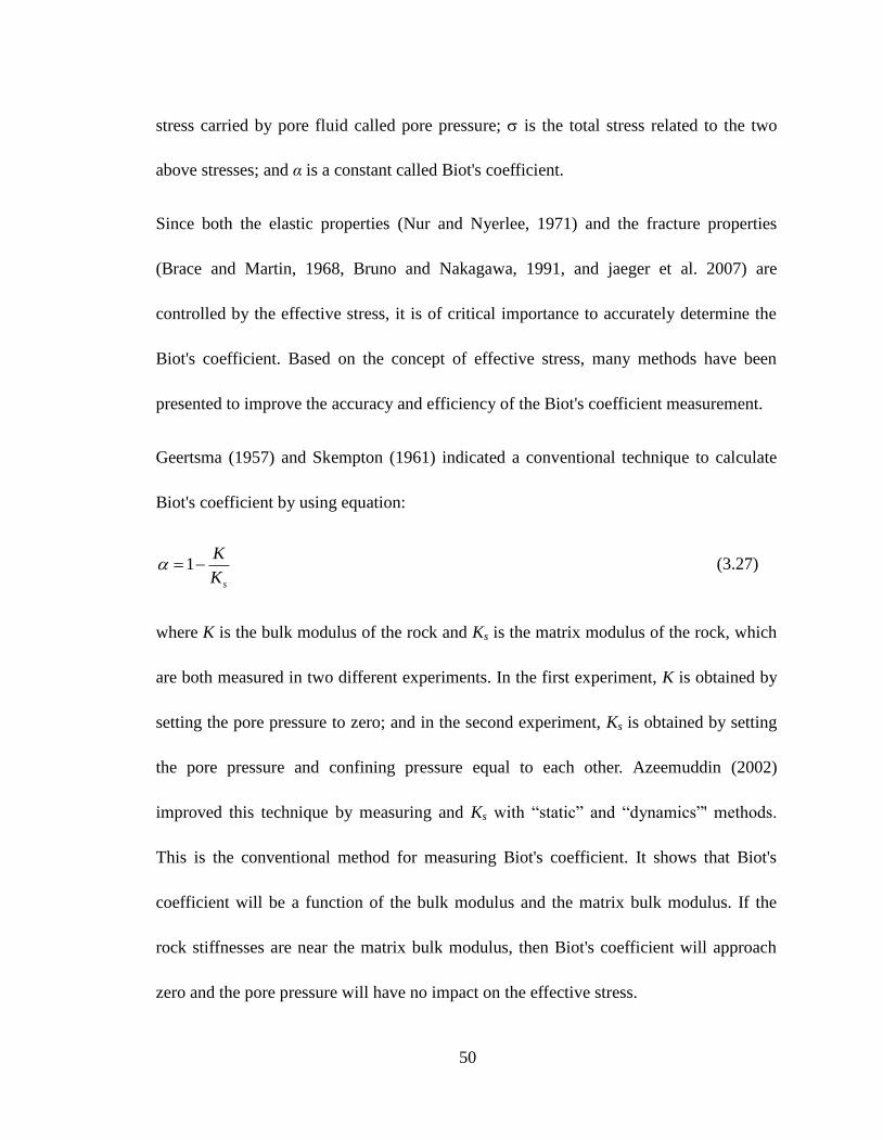
50
stress carried by pore fluid called pore pressure; is the total stress related to the two
above stresses; and α is a constant called Biot's coefficient.
Since both the elastic properties (Nur and Nyerlee, 1971) and the fracture properties
(Brace and Martin, 1968, Bruno and Nakagawa, 1991, and jaeger et al. 2007) are
controlled by the effective stress, it is of critical importance to accurately determine the
Biot's coefficient. Based on the concept of effective stress, many methods have been
presented to improve the accuracy and efficiency of the Biot's coefficient measurement.
Geertsma (1957) and Skempton (1961) indicated a conventional technique to calculate
Biot's coefficient by using equation:
1s
K
K (3.27)
where K is the bulk modulus of the rock and Ks is the matrix modulus of the rock, which
are both measured in two different experiments. In the first experiment, K is obtained by
setting the pore pressure to zero; and in the second experiment, Ks is obtained by setting
the pore pressure and confining pressure equal to each other. Azeemuddin (2002)
improved this technique by measuring and Ks with “static” and “dynamics”' methods.
This is the conventional method for measuring Biot's coefficient. It shows that Biot's
coefficient will be a function of the bulk modulus and the matrix bulk modulus. If the
rock stiffnesses are near the matrix bulk modulus, then Biot's coefficient will approach
zero and the pore pressure will have no impact on the effective stress.

51
Franquet (1999) proposed a technique to measure Biot's coefficient using equation:
pV
V
(3.28)
where ΔVp is the variation of the pore volume, and ΔV is the variation of the total rock
volume. Because these parameters are evaluated through measurement of the amount of
fluid volume drained from the rock sample, an accurate pore volume measurement is
needed. However, when testing the tight rock samples, we use gas instead of fluid due to
the low permeability; this method will cause leakage due to the long operating time.
Franquet (1999) also developed a “Mohr envelope” method to calculate the Biot's
coefficient, but this method needs several tests to define the envelope.
Qiao (2012) determined the Biot's coefficient under the assumption that the permeability
follows the effective-stress law. The author pointed out that the Biot's coefficient is a
function of the permeability, pore pressure, and confining pressure. However, it is
difficult to find the variation in permeability when the rock is tight. In this paper a new
method is proposed so that an experiment can be carried out and the result is easy to be
analyzed. This method simplified the measuring procedures to obtain the Biot coefficient
by recoding the variation of the confining pressure used to keep the volume of sample
constant while altering the pore pressure. In this proposed method, samples only need to
be measured once, which is fewer than conventional methods, whose procedures require
multiple core samples. Therefore, the proposed method can be accomplished

52
significantly quicker.
Measurement Principle
To better understand the new Biot's coefficient measurement, it is necessary to introduce
the derivation of the governing equation. The equation is derived by making the
following assumptions: the core is homogeneous, the properties of the rock are constant,
and the core and fluid are isothermal.
The bulk modulus of the rock is defined as the ratio of the change in stress to the strain,
expressed as follow:
v
K
(3.29)
where ∆σ΄ is the variation of the effective stress, and ∆εv is the variation of the
volumetric strain εv. Combining Equation 3.29 with Equation 3.26 we have:
( )p
v v
PK
Rearranging above equation, we get:
v
p
K
P
(3.30)
Equation 3.30 can be simplified if we can make ∆εv zero, which means the volume of
the rock sample is constant, and assuming K is constant.

53
pP
(3.31)
Figure 3.19 Schematic diagram of Biot's coefficient measuring process
Figure 3.19 shows the theoretical procedure. Once equilibrium has been attained, the
pore pressure is increased PP at time “A”. This causes a decrease in the volumetric strain
εv. The volumetric strain εv then returns to its original value at time “B” as the confining
pressure Pc is increased ∆Pc. Finally, the Biot's coefficient can be calculated as a ratio as
shown in Equation 3.31.
Measurement Procedure
Two problems arise when performing this experiment: 1). determine whether the volume
of the sample has changed or not; 2). determine the magnitude that the confining pressure
needs to be increased ∆Pc after the pore pressure has been increased ∆PP to return the
volumetric strain εv back to its original value. These problems can be solved with the
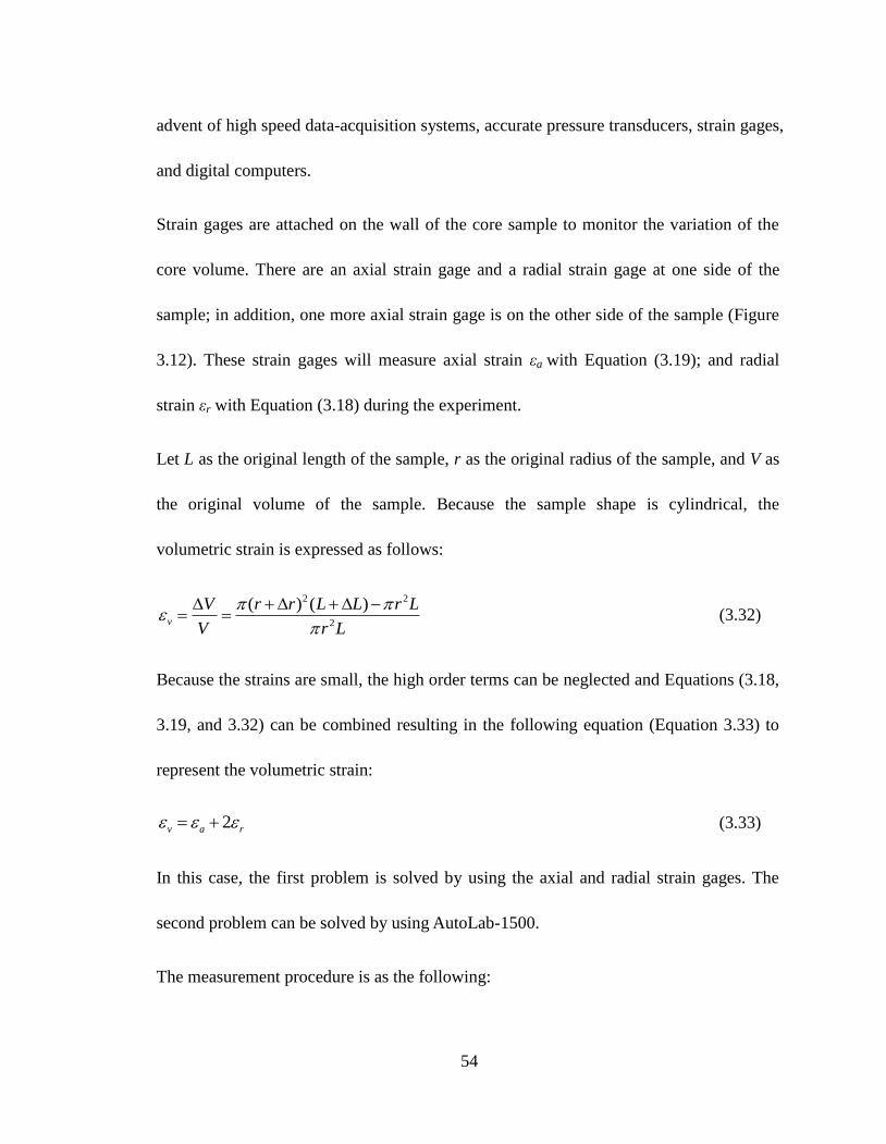
54
advent of high speed data-acquisition systems, accurate pressure transducers, strain gages,
and digital computers.
Strain gages are attached on the wall of the core sample to monitor the variation of the
core volume. There are an axial strain gage and a radial strain gage at one side of the
sample; in addition, one more axial strain gage is on the other side of the sample (Figure
3.12). These strain gages will measure axial strain εa with Equation (3.19); and radial
strain εr with Equation (3.18) during the experiment.
Let L as the original length of the sample, r as the original radius of the sample, and V as
the original volume of the sample. Because the sample shape is cylindrical, the
volumetric strain is expressed as follows:
2 2
2
( ) ( )v
V r r L L r L
V r L
(3.32)
Because the strains are small, the high order terms can be neglected and Equations (3.18,
3.19, and 3.32) can be combined resulting in the following equation (Equation 3.33) to
represent the volumetric strain:
2v a r (3.33)
In this case, the first problem is solved by using the axial and radial strain gages. The
second problem can be solved by using AutoLab-1500.
The measurement procedure is as the following:

55
1) Install the sample into AutoLab-1500 (like the permeability test part)
a. Mount the sample in a core holder with flexible rubber sleeves at both
ends of the plug (Figure 3.8). Connect the upstream end-cap to a
servo-controlled hydraulic intensifier, which is used to control and
monitor the upstream pressure. The downstream pressure at the other end
of the sample is monitored by a miniature pressure transducer, which is
located in the downstream end-cap.
b. Put the core holder into the pressure vessel, which is filled with mineral
oil, and apply confining pressure to a desired level.
c. Fill the upstream reservoir with dry nitrogen. Because the permeability of
Bakken sample is low, gas is used as the test fluid in the experiment.
d. Connect the upstream reservoir with the sample to the downstream
reservoir.
e. Increase the upstream pressure to a desired level.
f. Wait until the equilibrium of the downstream and upstream pressure
reached.
2) Configure AutoLab-1500 system to the confining pressure self-adjusting mode so
that the volumetric strain will keep constant
3) Increase the upstream pressure to the next level.
4) Wait until both the downstream pressure and the confining pressure reach their
new equilibrium.

56
5) Record the variations of confining pressure and pore pressure, respectively.
6) Repeat 3) to 5) by increasing or decreasing the upstream pressure. Figure 3.20
shows one record of the experiments.
7) Remove the sample from the core holder, and disconnect the core from the
end-caps.
Figure 3.20 Recording curves in one experiment
Table 3.2 Biot’s coefficient test on one sample
Pore Pressure
(MPa)
Confining Pressure
(MPa) Biot’s
Coefficient from to from to
6.20 8.20 22.87 24.27 0.70
8.20 10.20 24.27 25.77 0.75
10.20 12.30 25.77 27.09 0.63
Average 0.69
The results of the experiment recorded by Figure 3.20 are summarized in Table 3.2. After
57
the pre-equilibrium was achieved at pore pressure of 6.2 MPa and confining pressure of
22.87 MPa, the pore pressure was increased to 8.20, 10.20, and 12.30 MPa. To keep the
volume of the sample constant, the confining pressure is raised to 24.27, 25.77, and
27.09 MPa automatically by AutoLab-1500. The Biot’s coefficient of the sample then
was obtained from Equation 3.31. The average Biot’s coefficient of the sample is 0.69.
3.4.4. Compressive Strength
After all non-destructive were completed, we measured the compressive strength of
Bakken sample with triaxial compression test. The equipment used to do triaxial
compression test is AutoLab-1500.
The tri-axial compression test was done with a much lower deformation rate (0.005 mm
per minute), the confining pressure is kept constant, and the axial stress in the loading is
increased until the sample failed. The peak axial strength was recorded. The procedure
for conducting the experiment is almost the same as the measurement of static Young’s
modulus, except that no strain gage was used and velocity transducers are not in the
end-caps in this experiment. The following shows the procedure:
1) Jacket the sample with copper foil.
2) Insert the jacketed sample into the pressure vessel.
3) Fill the pressure vessel with mineral oil.
4) Increase the confining pressure to designed level.
5) Increase the differential stress and the confining pressure to the initial value for

58
the tri-axial compression measurement.
6) Set the loading rate.
7) Start tri-axial compression test, and collect the data.
8) End tri-axial compression test when the sample failed.

59
CHAPTER IV
EXPERIMENTAL RESULTS AND ANALYSIS
4.1. Porosity
4.1.1. Experiment Result
The porosity was measured successfully for 237 specimens among the total 240 Bakken
specimens. The mean porosity of the specimens is 4.922% with a standard deviation
1.578 (Table 4.1). The porosity is normal distribution (Figure 4.1). Moreover, the
porosity means of the Upper, Middle and Lower Bakken are low, in the range from 4 to
6%; and the Lower Bakken has the highest porosity and smallest distribution range,
which is shown clearly in Figure 4.2.
Table 4.1 Statistic results of porosity test
Member of Bakken
Formation
Total
Numbers
Success
Numbers
Porosity (%) Standard
Deviation Min Mean Max
Upper Bakken 42 40 0.800 4.265 7.900 2.088
Middle Bakken 140 139 1.900 4.792 8.7 1.381
Lower Bakken 58 58 2.200 5.688 10.400 1.329
Total 240 237 0.800 4.922 10.400 1.578

60
Figure 4.1 Histogram of porosity from 237 Bakken samples
Figure 4.2 Boxplot of the porosity for three members of Bakken Formation

61
4.1.2. Impact of Freezing
Recall that the freezing sample method is used in preparing the plug to overcome the
sampling difficulty. It is undoubted that the freezing will alter the rock texture and
structure thus the rock properties such as porosity and permeability, but like discussed
before, to the best of our knowledge it is the most successful approach to prepare the
shale core sample for lab test. Therefore, to obtain original rock properties, it is
imperative to quantify the difference before and after the freezing. Here we investigated
how the porosity changes during freezing process as below.
The effect of temperature on elastic properties of porous materials had been studied by
researchers of different fields, including petroleum engineering, civil engineering, and
chemical engineering. For the purposes of this research we reviewed the studies that
focused on the porosity change as a function of temperature. These researches can be
classified into two main categories according to temperature below and above ice melting
point (or water freezing point). The first category targeted temperature higher than ice
melting point (or water freezing point). Another investigated temperature is lower than
ice melting point under which the expansion of ice becomes the main cause that alters the
rock properties. Followings list some important researches that can be identified as
milestones that advance the understanding of effect of temperature on rock properties.
Somerton et al. (1965) studied the thermal effect on sandstone in the range of 400 to 800
oC. Their works showed that large changes in physical properties occur as a result of
62
heating and subsequent cooling to room temperature. They believed that the alteration of
rock properties is caused by a number of reactions occur during heating, which include
the differential thermal expansion of the quartz grains, the dissociation of dolomite at
higher temperatures, and the “firing” of clays at lower temperatures. Sanyal et al. (1974)
investigated the effect of temperature on petrophysical properties of reservoir rocks.
From their literature review, there was no definite result known about the effect of
temperature on porosity. The bulk volume increases slightly (<1%) with temperature
increase up to 200 oC. However, a cubic pore model was analyzed to simulate the change
in pore structure due to thermal expansion of mineral grains and cement. The expansion
of the grain spheres and the quartz cement due to temperature increase was calculated
using the thermal expansion coefficients of quartz. Different degrees of cementation were
considered in the model. Change of pore radius at different temperature levels were
obtained by subtracting new cement thickness from new grain radius. Vodak et al. (2004)
studied the effect of temperature on strength-porosity relationship for concrete material at
various temperatures ranging from 25 to 280 oC. Their study depicted that porosity
increases as a result of microcracking mainly due to thermal incompatibility of hardened
cement paste and aggregate during heating. Tian et al. (2009) obtained similar results in
their experimental studies on sandstone, claystone, clayey sandstone, and sandy
claystone where specimens were heated up to 1000 oC. It was observed that cracks were
generated on the rock samples, especially claystone, due to the difference in thermal
expansion properties of different minerals in the rock. Yao et al. (2012) and Hu et al.
63
(2012) presented further investigations on the microcracking mechanism during the
procedure of heating rock and coal samples. In general, at the initial heating stage,
increasing of temperature leads to the expansion of rock matrix, but the temperature is
not high enough to generate microcracks. Therefore, at the initial heating stage, the
porosity would slightly drop, or keep constant because of expansion of matrix and the
inelastic property preventing restoration of deformation when specimens are cooled to
ambient temperature. As the temperature continuously increases, the induced thermal
stress reaches and exceeds the strength of matrix, thus leads to the generation of
microcracks and increase of porosity. Therefore, there exists a “threshold temperature”,
where the sudden jump of porosity is observed, as the thermal stress becomes higher than
the matrix strength and creates cracks in rocks. Yuan et al. (2012) conducted
experimental study and simulated the effect of temperature on the voids in cement under
high pressure and high temperature conditions.
The other studies have paid attention to the effect of freezing on rock properties. Hundere
(1984) investigated the changes of unconsolidated core properties after freezing. Kindt
(1985) studied the effect of freezing on permeability of unconsolidated sandstone
through experimental measurement. Torsaeter and Beldring (1987) analyzed the effect of
freezing on permeability of unconsolidated to slightly consolidated rocks and core plugs.
Increasing in porosity, which ranges from 0.7% to 9.6%, was observed in their
experimental data. Neaupane et al. (1999) presented a coupled thermo-hydro-mechanical

64
model to simulate the freezing and thawing process. Their study focused on the effect of
phase change of pore water on the deformation of material. No discussion of the change
of porosity by freezing is available in the paper. Coussy (2005) studied the
poromechanics of freezing materials. The study focused on the liquid saturation degree
as a function of temperature, and ice-dependent poroelastic properties.
From the descriptions above, most of the previous researches focused on the high
temperature effect, or the effect of phase change of the pore water on the matrix structure
in freezing process. The induced thermal stress due to freezing may result in fractures. It
is expected that there also exists a “threshold temperature” during freezing, where sudden
change of porosity due to fracturing would be observed. Some of aforementioned
researches compared the rock or specimen porosity before and after freezing, and the
porosity change with the variation of temperature.
Unfortunately it is unfeasible to measure porosity of Bakken shale core plug before
freezing, because the Bakken shale core has to be frozen in order to drill plug
successfully due to its brittle nature. In this case, we quantified the difference in rock
porosity before and after the freezing basing on experimental data from numerous rock
specimens. To do so, porosities of the samples were measured before they were frozen.
Then samples were stored in freezer and frozen at temperatures of -13.8 and -85 oC for
more than one week. After that they were taken out of freezer and allowed to return to
temperature of 20 oC. Their porosities were measured again once temperature reaches

65
equilibrium.
Table 4.2 Porosity change caused by freezing
Samples Diameter Length Porosity Φ(%) (Φ-Φ20)/Φ20
mm mm 20 oC -13.8
oC -85
oC 20
oC -13.8
oC -85
oC
1 23.54 42.25 12.512 19.197 14.127 0.000 0.534 0.129
2 24.3 51.55 10.969 14.472 14.579 0.000 0.319 0.329
3 24.65 28.44 16.624 21.496 18.006 0.000 0.293 0.083
4 24.69 49.98 11.296 13.764 12.620 0.000 0.218 0.117
5 24.25 52.58 12.755 14.770 13.886 0.000 0.158 0.089
6 24.38 52.69 13.504 14.968 14.168 0.000 0.108 0.049
7 24.67 55.25 16.481 17.941 18.068 0.000 0.089 0.096
8 24.69 52.6 13.501 14.694 14.470 0.000 0.088 0.072
9 24.95 51.05 18.478 20.029 18.870 0.000 0.084 0.021
10 24.73 51.56 18.807 20.302 19.698 0.000 0.079 0.047
11 24.82 51.55 15.057 15.976 15.531 0.000 0.061 0.031
12 38.44 76.15 13.999 14.759 14.574 0.000 0.054 0.041
13 24.65 58.38 17.068 17.952 17.770 0.000 0.052 0.041
14 38.08 74.33 12.958 13.583 13.784 0.000 0.048 0.064
15 38.43 76 13.382 14.006 13.832 0.000 0.047 0.034
16 38.43 76.26 14.868 15.534 15.574 0.000 0.045 0.047
17 24.45 53.91 22.483 23.485 23.491 0.000 0.045 0.045
18 38.48 76.18 12.114 12.652 12.090 0.000 0.044 -0.002
19 38.42 76.25 13.699 14.209 14.493 0.000 0.037 0.058
20 38.25 75.21 13.212 13.646 13.804 0.000 0.033 0.045
21 38.47 74.14 13.728 14.125 13.931 0.000 0.029 0.015
22 24.76 46.6 12.995 13.364 14.038 0.000 0.028 0.080
23 38.38 75.77 13.778 14.138 13.951 0.000 0.026 0.013
24 25 51.95 15.194 15.569 16.415 0.000 0.025 0.080
25 38.42 76.26 13.802 14.134 14.209 0.000 0.024 0.029
26 24.63 50.37 22.060 22.566 24.060 0.000 0.023 0.091
27 24.81 49.62 15.094 15.311 15.583 0.000 0.014 0.032
28 38.44 76.05 14.238 14.350 14.268 0.000 0.008 0.002
29 24.3 52.37 12.875 12.953 15.676 0.000 0.006 0.218
30 24.27 52.95 17.583 17.684 18.736 0.000 0.006 0.066

66
Table 4.2 Cont
31 50.12 102.78 14.963 15.028 14.905 0.000 0.004 -0.004
32 38.47 76.14 12.412 12.426 12.603 0.000 0.001 0.015
33 50.27 105.05 15.611 15.591 15.491 0.000 -0.001 -0.008
34 38.3 75.81 13.334 13.279 13.177 0.000 -0.004 -0.012
35 38.2 76.15 13.547 13.453 13.512 0.000 -0.007 -0.003
36 50.16 102.78 15.057 14.910 14.936 0.000 -0.010 -0.008
37 25.68 50.31 21.884 21.660 22.118 0.000 -0.010 0.011
38 50.24 103.43 15.681 15.510 15.562 0.000 -0.011 -0.008
39 38.46 76.03 14.976 14.803 14.600 0.000 -0.012 -0.025
40 38.35 76.25 14.156 13.959 14.192 0.000 -0.014 0.003
41 38.46 78.17 16.881 16.635 16.845 0.000 -0.015 -0.002
42 24.78 50.78 16.586 16.338 16.901 0.000 -0.015 0.019
43 24.47 48.81 11.164 10.917 15.535 0.000 -0.022 0.392
44 24.84 48.97 15.599 15.234 15.533 0.000 -0.023 -0.004
45 38.45 76.15 14.352 13.970 13.954 0.000 -0.027 -0.028
46 24.5 52.55 15.155 14.658 15.408 0.000 -0.033 0.017
47 24.08 51.48 15.224 14.713 15.698 0.000 -0.034 0.031
48 24.17 50.09 9.821 9.386 13.411 0.000 -0.044 0.366
49 24.74 51.49 16.681 15.858 17.042 0.000 -0.049 0.022
50 24.58 51.65 13.062 12.199 15.665 0.000 -0.066 0.199
51 24.83 51.85 16.718 15.605 16.960 0.000 -0.067 0.014
52 24.8 50.45 15.283 14.235 17.547 0.000 -0.069 0.148
53 24.65 52.67 12.503 11.583 15.378 0.000 -0.074 0.230
54 24.17 50.45 11.694 10.684 13.892 0.000 -0.086 0.188
55 24.4 52.27 11.843 10.799 13.288 0.000 -0.088 0.122
56 24.25 52.56 13.886 12.305 16.040 0.000 -0.114 0.155
Two series of different size specimens were used in this work. The first series has a
dimension of one inch in diameter by two inches in length, and another has a dimension
of two inches in diameter by four inches in length. The porosities of rock before and after
freezing were measured. Thus we obtain three porosities for each specimen: one before

67
freezing, one after freezing at -13.8 oC, and one after freezing at -85
oC.
To demonstrate the change of porosity by freezing distinctly, we calculate the relative
porosity change using porosity of rocks at 20 oC as the base. Table 4.2 shows the
experiment results.
Figure 4.3 Regression analysis of porosity change caused by freezing
Based on the test data, three kinds of porosity change by freezing can be identified as
shown in Figure 4.3, and they are corresponding to different types of rocks. For the first
type (a), whose lithology is argillaceous sandstone, the porosity increases as the rock was
frozen, and reaches maximum at temperature barely lower than 0 0C. After that local
maximum, porosity declines as temperature is reduced further. For the second type (b),
whose lithology is clean sandstone, the trend is similar to first type but with smaller

68
change. The porosity change by freezing is very small until temperature reaches the
“threshold temperature”, beyond that point the porosity begins to increases quickly. The
third type (c), whose lithology is sandstone with high calcium carbonate concentration,
follows the same trends as first and second types. A local maximum porosity is seen at
temperature barely lower than 0 0C, but the change of porosity lies between first and
second types. A “threshold temperature” also can be found as the temperature decrease
continuously. The porosity increases again when the temperature is lower than the
“threshold temperature”.
Porosity change is the combined effects of expansion of the water inside the core due to
phase change and the contractions of the matrix of the core and ice. When the core is
stored in freezer at temperature lower than freezing point, the freezing causes the water
inside the core to expand due to the fact that ice occupies a larger volume than liquid
water. The relative volume change is
expansion8.7%ice water
water water
V V V
V V
(4.1)
The expansion volume due to water phase change is
expansion ,0.087 0.087water w bulk coreV V S V (4.2)
During the freezing, both ice and rock matrix contract. The volume change due to the
contraction can be estimated using the thermal expansion coefficient. The contraction
volumes of ice and rock matrix are calculated by

69
contraction,ice ice freezing point freezer ice
, freezing point freezer ice1.087 w bulk core
V V T T
S V T T
(4.3)
and
contraction,matrix ,min eral freezing point freezer ,mineral
, ,mineral freezing point freezer ,mineral1
n
i i
i
n
bulk core i i
i
V V T T
V f T T
(4.4)
respectively.
where
6 o
ice 50 10 1/ C
and the coefficients of thermal expansion of different minerals are listed in Table 4.3.
Table 4.3 Thermal expansion coefficients of common minerals in rock
Mineral Thermal Expansion
Coefficient Reference
Quartz 0.77~1.4×10⁻⁶
1/oC
http://www.engineeringtoolbox.com/linear-expansion-coeffi
cients-d_95.html
Alkali Feldspar 14~17×10-6
1/oC
Hovis, G., et al., 2008, A simple predictive model for the
thermal expansion of AlSi3 feldspars.
Plagioclase
Feldspar 10~17×10
-6 1/
oC
Tribaudino, M., et al., 2010, Thermal expansion of
plagioclase feldspars:
Calcium
Carbonate 6~9×10
-6 1/
oC http://www.supercivilcd.com/THERMAL.htm
Calcium
Carbonate 8×10
-6 1/
oC
http://www.engineeringtoolbox.com/linear-expansion-coeffi
cients-d_95.html
Combing Equations (4.2), (4.3), and (4.4) we have the total volume change, which is

70
contraction,ice contraction,matrix expansion
freezing point freezer ice
, ,min eral freezing point freezer ,min eral
1.087
1
0.087
total
w
n
bulk core i i
i
w
V V V V
S T T
V f T T
S
(4.5)
Therefore the relative volume change is
freezing point freezer ice
,min eral freezing point freezer ,min eral
,
1.087
1
0.087
w
ntotal
i i
ibulk core
w
S T T
Vf T T
V
S
(4.6)
Equation (4.6) gives the incremental porosity at freezer temperature. So the rock porosity
at freezer temperature is
freezing point freezer ice
,min eral freezing point freezer ,min eral
1.087
1
0.087
w
n
freezer temperature i i
i
w
S T T
f T T
S
(4.7)
If the induced stress is less than the adhesive strength of rock and the rock is elastic, the
rock should restore to its original condition when the temperature is restored to original
temperature. Unfortunately no rock is completely elastic. Therefore rock cannot restore
to its original condition exactly even the rock is not damaged by the induced stress. The
residual porosity difference as a result of freezing-unfreezing cycle depends on the water
and the percentage of inelastic component in rock.
If the induced stress is higher than the adhesive strength of rock, rock porosity after

71
freezing-unfreezing cycle will be larger than the original porosity because the
microcracks and plastic component in the rock prevent the rock from restoring to
original condition when temperature return to original value. To evaluate the occurring of
microcrack it is necessary to introduce the definition of volumetric strain, which is
defined as the ratio of the change in volume of the body to its original volume (Jaeger, et
al., 2007).
V
original
V
V
(4.8)
Recalling that the volumetric strain is the sum of the three principal normal strains we
have
V 1 2 3 (4.9)
The relationships between the three principal normal stresses and strains give us
1 V 12G (4.10)
2 V 22G (4.11)
3 V 32G (4.12)
Summing up the three principal stresses gives
1 2 3 V3 3 2m G (4.13)
The mean stress is related to the volumetric strain through

72
V
freezing point freezer ice
,min eral freezing point freezer ,min eral
2
3
1.087
21
3
0.087
m
w
n
i i
i
w
G
S T T
G f T T
S
(4.14)
where
2
1 2
Gv
v
(4.15)
If the mean stress calculated from Equation (4.14) is higher than adhesive strength of
rock, micorcrack will be created and increase in porosity will be expected.
Analysis of experimental data indicates that there is a “threshold temperature” for rock.
When the rock is frozen at temperature high than “threshold temperature” and restored to
original temperature, porosity decreases. Otherwise porosity increases. At temperature
between freezing point and “threshold temperature”, the expansion resulting from water
phase change to ice dominates over the contractions of rock matrix and ice. The
expanded volume is larger than the contracted volume. The deformation occurring at this
temperature range is partially inelastic and the rock cannot restore to original condition
even temperature is restored to original temperature. It should be noted that the induced
stress is below the adhesive strengths between cements and grains or the strength of
matrix under this temperature range. At temperature lower than the “threshold
temperature”, the contractions of ice and rock matrix dominates over the expansion due
to the water phase change. The induced thermal stress resulting from strain caused by

73
contraction reaches and exceeds the adhesive strengths between cements and grains or
the strength of matrix, thus lead to the creation of microcracks. These microcracks are the
main reason porosity increases. Under such condition the expanded volume is smaller
than the contracted volume. The deformation is damaging and irreversible, and again the
rock cannot restore to original condition after temperature is restored to original
temperature. Obviously the “threshold temperature” is a function of rock type, rock
structure, texture, mineral composition, rock strength, water saturation, mineral hydration,
and porosity. To calculate an accurate porosity change, it is necessary to know the
volumetric fraction of minerals in rock, as well as the coefficient of thermal expansion of
each mineral.
4.2. Permeability
4.2.1. Experiment Result
Permeability was measured for all 240 Bakken specimens using the Oscillating Pulse
method with the AutLab-1500 (Boitnott 1997). The confining pressure and pore pressure
are 30 MPa and 8 MPa, respectively. The success rate of test is about 85.5%. The median
permeability of the specimens is 0.63 µD with a standard deviation 5169.97 (Table 4.4).
Figure 4.4 shows that the permeability of the Middle Bakken is lower than that from
Upper and Lower Bakken; moreover the permeabilities of the Upper Bakken and the
Lower Bakken spread widely, even have much large permeability. These features may
cause by the fractures in the Upper and Lower shale core plugs. Based on this hypothesis,

74
we not only investigated the existing methods to ascertain fractures, but proved one
method to identify fractures in tight rocks with porosity-permeability relation as well.
Table 4.4 Statistic result of permeability test
Member of
Bakken
Formation
Total
Numbers
Success
Numbers
Permeability (µD) Standard
Deviation 1st
Quarter Median Mean
3rd
Quarter
Upper Bakken 42 33 6.79 239.00 6613.00 6760 10551.83
Middle Bakken 140 121 0.07 0.30 127.47 1.87 672.83
Lower Bakken 58 51 0.08 1.45 1185.67 72.40 3848.31
Total 240 205 0.09 0.63 1434.78 44.00 5169.97
Figure 4.4 Boxplot of the porosity for three members of Bakken Formation
4.2.2. Identify fractures with porosity-permeability relation
Identification of fractures in the rock is critical in rock characterization and important to
design multistage fracturing in horizontal well to maximize the production. Knowing the
fracture direction helps determine the direction of horizontal lateral to maintain wellbore

75
stability during drilling and create long fractures in multistage fracturing. Therefore
methods that can identify fractures and determine their directions are highly desired.
Nelson (1976) conducted experiment to investigate the effect of temperature and
confining pressure on fracture permeability in Navajo sandstone. Fertl and Rieke (1980)
identified fractured shale by gamma ray spectral evaluation techniques. Thorpe (1981)
characterized natural fractures in granitic rock using observation method. Brown and
Scholz, (1985), Cart and Warriner (1987), Aviles, et al. (1987), applied fractal geometry
to the objective description of rock fracture surfaces. Dennis and Slanden (1988) used
imaging techniques consisting of Formation MicroScanner log and the Borehole
Televiewer to locate the fracture on wellbore. Locker (1993) tracked the growth and
interaction of microcracks using acoustic emission. Feng et al. (1958) mapped the
fracture at exposed rock faces by applying close rang digital photogrammetry and
geodetic total station. Labuz and Chen (2001), and Lin and Labuz (2010) utilized
nondestructive technique of electronic speckle pattern interferometry to monitor the
propagation of fracture initiated by a wedge indenter. Their experiments on Berea
sandstone and Sioux quartzite showed a good agreement between the cavity expansion
model and the experiments in terms of indentation pressure and size of the damage zone
located beneath the indenter. El-Gezeery et al. (2008) employed real time logging while
drilling resistivity imaging to identify fracture corridors in a fractured carbonate reservoir.
Lin and Fairhurst (1991) used principle of combinatorial topology to analyze the
three-dimensional network of fracture. Bravo and Aldana (2011) used different volume

76
curvature attributes to identify subtle faults and fractures in carbonate reservoirs. Han
(2011) proposed an integrated method including electrical image tools such as well
logging, core observation, production logs, and rate transient analysis, and outcrop
observation to identify fractures. Stanchits et al. (2012) monitored the propagation of
hydraulic fracture in heterogeneous rock samples using acoustic emission and ultrasonic
transmission. Salehi and Ciezobka (2013) identified natural fractures in shale reservoir
through the analysis of surface pumping parameters. Their analyses were confirmed by
microseimic data and multiple production logs. Although imaging methods and other
technologies have been used to characterize the fracture distribution, they are time
consuming and expensive, and sometimes are constrained by the availability of
equipment.
According to a capillary tube model of porous media (Ling, 2012), which should be
followed by all fluid flow behaviors in the non-fractured core sample, the permeability is
proportional to the square of porosity and inversely proportional to the cubic of tortuosity
of rock. And empirical observations give a general relation between porosity and
permeability as follow:
nk Ce (4.16)
where C is a constant linear coefficient, and n is exponential coefficient.
It should be noted that C and n vary with different lithology. Same types of rocks share
similar C and n unless there is/are fracture/s within them considering a small fracture can
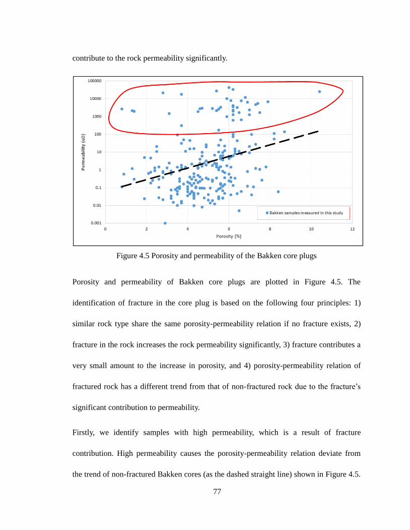
77
contribute to the rock permeability significantly.
Figure 4.5 Porosity and permeability of the Bakken core plugs
Porosity and permeability of Bakken core plugs are plotted in Figure 4.5. The
identification of fracture in the core plug is based on the following four principles: 1)
similar rock type share the same porosity-permeability relation if no fracture exists, 2)
fracture in the rock increases the rock permeability significantly, 3) fracture contributes a
very small amount to the increase in porosity, and 4) porosity-permeability relation of
fractured rock has a different trend from that of non-fractured rock due to the fracture’s
significant contribution to permeability.
Firstly, we identify samples with high permeability, which is a result of fracture
contribution. High permeability causes the porosity-permeability relation deviate from
the trend of non-fractured Bakken cores (as the dashed straight line) shown in Figure 4.5.

78
The high permeability samples that may contain fractures are marked by the red circle,
and samples outside of red circle are believed to be fracture free. To develop the
porosity-permeability relation for non-fractured core plugs, samples outside of red circle
in Figure 4.5 are used to regress to estimate coefficients, C and n, in Equation 4.16. The
regression gives C=0.0394 and n=0.5412 as shown in Figure 4.6. Therefore, the
porosity-permeability relation for non-fractured Bakken cores becomes
0.54120.0394k e (4.17)
To better understand the porosity-permeability relation of fractured Bakken cores,
samples inside the red circle in Figure 4.5 are used to construct the relation and to
evaluate coefficients, C and n, the plot in Figure 4.7 indicates that C=1977.9 and
n=0.1153 for fractured cores, which are significantly different from those of
non-fractured core correlation. The porosity-permeability relation for fractured Bakken
cores becomes
0.11531977.9k e (4.18)

79
Figure 4.6 Porosity-permeability relation developed from core plugs without fracture
Figure 4.7 Porosity-permeability relation developed from core plugs with fracture
Equations (4.17) and (4.18) put the foundation for identifying fracture in Bakken core
based on the porosity-permeability relation. It is reasonable to conclude that core with
porosity-permeability relation similar to Equation (4.17) does not contains fracture, while
core with porosity-permeability akin to Equation (4.18) contains fracture.

80
To validate the proposed method, visual observation on core plugs is applied to examine
if there are fractures developed in a sample. For the 39 samples that are classified as
fractured core plug based on porosity-permeability relation method, core observation
indicates that 37 samples of them contain fractures. Therefore, there is a high agreement
between porosity-permeability method and observation method.
Figure 4.8 Porosity-permeability of Bakken cores measured in this study and measured
by Corelab (Well#16089)
To further verify the proposed method, we overlapped other Bakken core data on Figure
4.5 as shown in Figure 4.8. These Bakken cores from well# 16089 (NDIC file name)
were analyzed by Corelab (Samson Resources Company, 2006). In core analysis,
porosity and permeability were measured; and the cores with fracture were identified
through observation. As shown in Figure 4.8, there are 39 cores from well# 16089 of

81
which 15 cores (green data) locate inside the fractured core zone. Corelab’s report
denotes that these 15 samples contain fractures or are chipped sample. The other 24
samples (brown data points) lie in non-fracture core zone. No fracture was observed in
these 24 samples according to Corelab’s report. Therefore, the identification of fracture
through the proposed model is reliable.
The developed method identifies fractures based on the permeability test under
unsteady-state flow. Since it relies on permeability test data only, it does not require
additional cost and equipment to conduct the test to generate images by imaging methods.
The proposed method provides a practical, simple, and very low cost way to identify and
characterize fractures in tight rocks. It can work as an important supplement to imaging
methods for unconventional reservoirs
4.2.3. Comparison of Three Permeability Methods
The oscillating method with the AutLab-1500 system performs sensitivity studies to
provide a means of computing errors associated with the insensitivity of the solution to
the separation of permeability and specific storage. However, the data analysis technique
is not shared by New England Research Inc.
To validate the permeability from the oscillating method, the permeabilities of six
Bakken core plugs were measured using the oscillating pulse method, the downstream
pressure build-up method, and the radius-of-investigation method. The pressure-time
graphs are shown in Figure 3.9, Figure B.1, and Figures D.1 through D.10.

82
Table 4.5 Main parameters and permeability results from three methods on Bakken core
plugs
unit Core 1 Core 2 Core 3 Core 4 Core 5 Core 6
L in 2.7780 2.7224 2.7008 2.3882 2.6992 2.5819
D in 1.0311 1.0394 1.0327 1.0323 1.0291 1.0315
ϕ fraction 0.044 0.045 0.032 0.035 0.036 0.054
cs 1/psi 0.000009 0.000009 0.000009 0.000009 0.000009 0.000009
cg 1/psi 0.000125 0.000125 0.000125 0.000125 0.000125 0.000125
ct 1/psi 0.000134 0.000134 0.000134 0.000134 0.000134 0.000134
μ cp 0.0293 0.0293 0.0293 0.0293 0.0293 0.0293
V2 ft3 2.22E-05 2.22E-05 2.22E-05 2.22E-05 2.22E-05 2.22E-05
s Ln(psi
2)
/h -2.781108 -1.3644 -1.818 -1.2528 -2.4228 -78.12
μ cp 0.0293 0.0293 0.0293 0.0293 0.0293 0.0293
t h 0.0694 0.28 0.13889 0.14167 0.05556 0.0035
k
(buildup) µD 0.1864 0.09 0.1164 0.0791 0.158 5.2731
k
(radius-of-in
vestigation)
µD 0.2527 0.0615 0.0868 0.0728 0.2438 5.3546
k
(oscillating
pulse)
µD 0.108 0.046 0.0724 0.0438 0.11 2.25
The parameters that were used in the tests and experiment results are shown in Table 4.5.
The permeabilities from the downstream pressure build-up method and the
radius-of-investigation method are close to those from the oscillating pulse method
(Figure 4.9). Therefore, the downstream pressure build-up method and the
radius-of-investigation method provide the same order of magnitude of permeability as
the oscillating pulse method for tight rocks. This indicates that the uncertainty has been
reduced materially. Figure 3.9 shows that the measured time of the

83
radius-of-investigation method (ends at point “B”) requires less time than the oscillating
pulse method (ends at point “C”).
Figure 4.9 Comparison of permeabilities as measured by the three methods
The pressure build-up method, which is based on the pulse-decay method, is the
transformation of a mature technique to measure the low permeability. Our study
managed to reduce the downstream reservoir volume as much as possible in order to
reduce the operation time. It requires less time than the oscillating pulse method and is
a faster alternative to the steady-state, commonly accepted method. It is worth
mentioning that to reduce the uncertainty during this procedure, the data that is chosen to
calculate the slope (s) should be part of the data between point “B” and “A” with high
signal-to-noise ratio (Figure 3.9). Because selecting the whole curve to fit will increase
slope (s), or using the earlier data to fit will significantly reduce slope (s) (Figure A.1),
middle data with high signal-to-noise ratio should be selected (Figure 4.10). Doing so
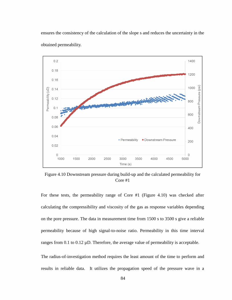
84
ensures the consistency of the calculation of the slope s and reduces the uncertainty in the
obtained permeability.
Figure 4.10 Downstream pressure during build-up and the calculated permeability for
Core #1
For these tests, the permeability range of Core #1 (Figure 4.10) was checked after
calculating the compressibility and viscosity of the gas as response variables depending
on the pore pressure. The data in measurement time from 1500 s to 3500 s give a reliable
permeability because of high signal-to-noise ratio. Permeability in this time interval
ranges from 0.1 to 0.12 µD. Therefore, the average value of permeability is acceptable.
The radius-of-investigation method requires the least amount of the time to perform and
results in reliable data. It utilizes the propagation speed of the pressure wave in a

85
certain media to calculate the permeability. This method provided a fast measurement of
the low permeability. The measurement time for this method is 10 times less than the
downstream pressure build-up method in this study. The radius-of-investigation method
not only can be used to measure low permeability, but also can be used to measure high
permeability by replacing the gas fluid with a liquid fluid. Other than the human
introduced random error, the major uncertainty source in this method is mainly from the
selection of point “B”. To reduce the uncertainty, the beginning of the responding time
(or point “B”) is manually selected. It is easy to identify the starting point of downstream
pressure build-up, which is point “B”, through amplifying the short time interval as
shown in Figure 3.9.
After we compared our results with those of Bertoncello’s investigation (2013), the
permeabilities from these three methods are close. This increases the confidence level.
Therefore, the comparative measurement and analysis has value by providing fast and
inexpensive measurements and can help quantify uncertainties.
In theory, the pore pressure differences in the three methods can cause the permeability
difference because high pore pressure leads to a larger pore volume and thus a higher
permeability. However, the results show that the lowest permeability is determined by
oscillating pulse method, which is under the highest pore pressure. The reason is that the
oscillating pulse method is proffered by AutLab-1500 system which considers the storage
of the sample; this implies that the porosity of the samples is a variable in this method,

86
and the porosity decreases with the effective pressure increase. However, for the other
two methods, in this study we assume that the value of porosity is constant. It is equal to
the one measured at 1 atm. In fact with effective pressure increase, porosity will be
reduced; thus, with a large porosity value, the permeability calculated by the other two
methods is greater than the actual permeability.
If the results from these three methods are not close, it will not always be the case that
the confidence level is low. It may indicate that the rock has a non-uniform pore structure.
The heterogeneity of rock and/or microcracks may be the main causes. Considering the
high pore pressure in the oscillating pulse and downstream pressure buildup methods and
low pore pressure in the radius-of-investigation method, the heterogeneity and lamination
of rock can be identified by the change of the permeability difference between the
oscillating pulse and downstream pressure buildup methods and the
radius-of-investigation method. The contribution of highly permeable parts of the rock
becomes more important in the oscillating pulse and downstream pressure buildup
methods than in the radius-of-investigation method as pore pressure increases. If
microcracks exist in the rock, the permeability difference between the oscillating pulse
and downstream pressure buildup methods and the radius-of-investigation method is
higher than those caused by heterogeneity and lamination because the increase in the
microcrack permeability is more significant than that in matrix permeability when pore
pressure increases. It should be noted that heterogeneity and lamination can be coupled

87
with microcracks in many rocks, and make the decoupling of the effects of heterogeneity
and lamination from microcracks very difficult. Therefore, further work needs to be done
to quantify or identify the causes of differences through advanced imaging technology.
4.2.4. Investigation of Pore Pressure Impact
Many researches proved that permeability is reduced when the confining pressure is
increased, depending upon the result of studying the effect of confining pressure on the
permeability of porous media (Fatt, 1952 and 1953, mclatchie 1958, Dobrynin 1962,
Zoback 1975). Although it is in general known that permeability declines as effective
stress is increased, none of the correlations between permeability and effective stress can
be used for all situations at the present time. Normally the change of effective stress is
caused by the pore pressure decrease due to the depletion of reservoir during the
production, and it is most difficult to measure Biot’s coefficient for low permeability
rocks, such as Bakken shale (He and Ling, 2014). Thus, a permeability-pore pressure
correlation developed from experimental data is still needed.
With the aim of identifying the effect of pore pressure on permeability of Bakken
samples, we have measured the permeability for 46 Bakken core plugs with Oscillating
Pulse Method under different conditions in the range of 20-40 MPa and 3.5-7.5 MPa for
the confining pressure and pore pressure, respectively. The confining pressure was
maintained constant as changing the pore pressure, in order to correlate the applied pore
pressure with the permeability and vice versa. The permeability measured in different

88
pressure conditions are shown in Figure 4.11.
Figure.4.11 Permeability of 46 Bakken samples measured under different pressure
Conditions
Figures 4.12, 4.13, 4.14, 4.15, and 4.16 are the distribution from of the permeability tests
under different pressure saturations with the 46 Bakken samples. Those Figures clearly
show that:
1) The most common permeability (80%) ranges from 0.001 µD to 1 µD.
2) The permeability increase as pore pressure increase. For instance, the percentage
of samples whose permeability are great than 1µD is increase from 17% to 18%
and 20%, as pore pressure increase from 3.5 MPa to 5.5 MPa and 7.5 MPa.
3) The permeability decrease as confining pressure increase. For instance, the

89
percentage of samples whose permeability are great than 1µD is decrease from 20%
to 15% and 9%, as confining pressure increase from 20 MPa to 30 MPa and 40
MPa.
Figure 4.12 Permeability distribution (Confining pressure =20MPa, pore pressure = 3.5
MPa).
Figure 4.13 Permeability distribution (Confining pressure =20MPa, pore pressure = 5.5
MPa).

90
Figure 4.14 Permeability distribution (Confining pressure =20MPa, pore pressure = 7.5
MPa).
Figure 4.15 Permeability distribution (Confining pressure =30MPa, pore pressure = 7.5
MPa).
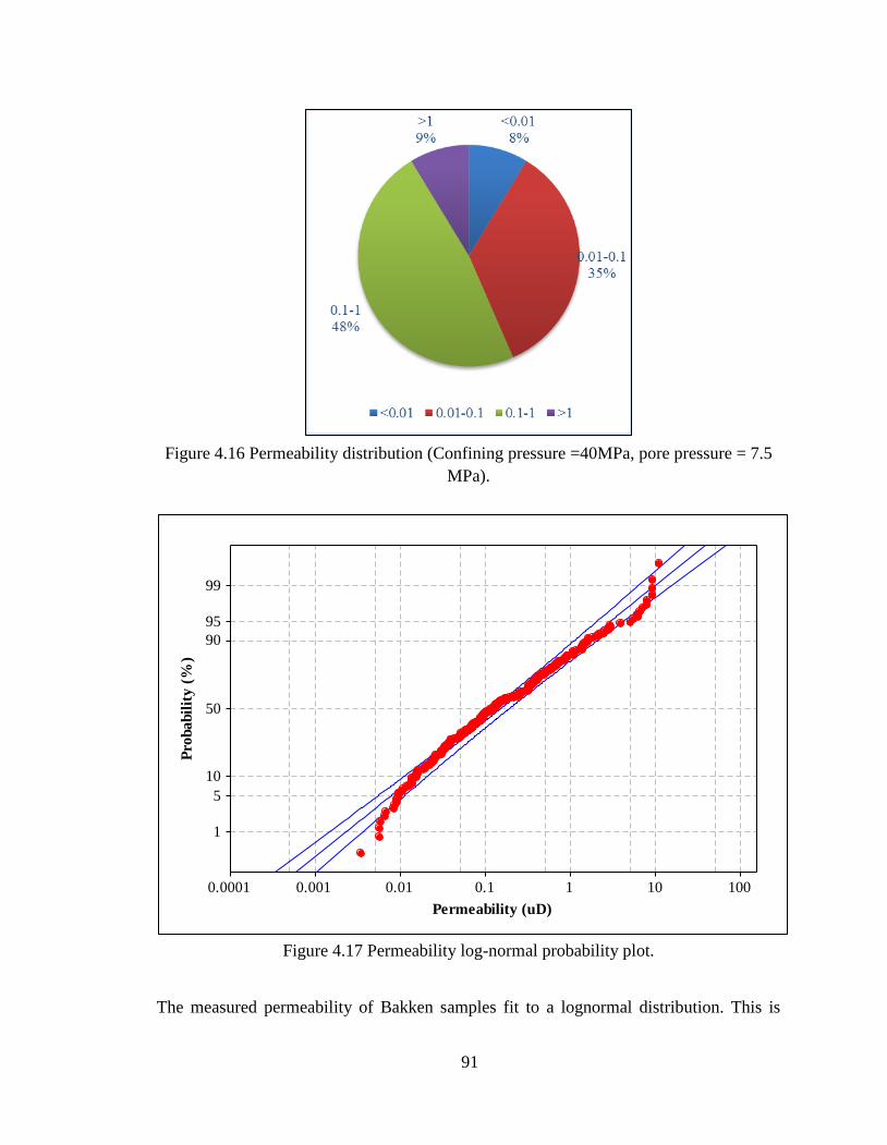
91
Figure 4.16 Permeability distribution (Confining pressure =40MPa, pore pressure = 7.5
MPa).
Figure 4.17 Permeability log-normal probability plot.
The measured permeability of Bakken samples fit to a lognormal distribution. This is
1001010.10.010.0010.0001
99
95
90
50
10
5
1
Permeability (uD)
Pro
babil
ity
(%
)

92
proved by the close fit of the data to a straight line as shown in Figure 4.17.
Table 4.6 contains the statistics of measured permeability with lognormal distribution.
Those statistics strongly support that:
1) There is a proportional relationship between permeability and pore pressure. The
evidence is that with a constant confining pressure as 20 MPa, the mean value of
permeability increases from 0.122 µD to 0.175 µD and 0.199 µD when the pore
pressure increased from 3.5 MPa to 5.5 MPa and 7.5 MPa, respectively. Moreover,
the 95% confidence intervals for those three different pore pressure conditions are
from 0.069 to 0.216 µD, 0.101 to 0.303 µD, and 0.117 to 0.337 µD, respectively.
2) Permeability is inversely proportional to confining pressure. With a constant pore
pressure as 7.5 MPa, the mean value of permeability is decreases from 0.199 µD
to 0.136 µD and 0.133 µD when the confining pressure increased from 20 MPa to
30Mpa and 40MPa, respectively. And the 95% confidence intervals for those
three different confining pressure conditions are from 0.117 to 0.337 µD, 0.081 to
0.228 µD, and 0.080 to 0.221 µD, respectively.
Table 4.6 Statistics analysis of permeability of Bakken samples
Pore
Pressure
Confining
Pressure
Permeability
(µD)
(MPa) (MPa) Mean Variance Min Max 95% Confidence
Interval
3.5 20 0.122 4.920 0.006 9.036 0.069 0.216
5.5 20 0.175 4.426 0.009 9.120 0.101 0.303
7.5 20 0.199 3.954 0.011 10.765 0.117 0.337
7.5 30 0.136 3.715 0.006 6.152 0.081 0.228
7.5 40 0.133 3.581 0.003 6.281 0.080 0.221

93
To develop the relation between the permeability and both of pore pressure and confining
pressure, the mean values of permeability are used to regress. One regression equation is
given as:
0.1443 0.0036 0.0163c pk p p (4.19)
and the R2 of this regression equation is 0.8.
Equation (4.19) shows that permeability (K) will be reduced when the confining pressure
(pc) is increased, and the reduction factor from the confining pressure is 0.0036; on the
other hand, permeability will be increased with the pore pressure increase, and the
increment factor for the pore pressure is 0.0163. Thus, the pore pressure has a greater
influence on permeability than the confining pressure has.
4.3. Elastic Moduli
4.3.1. Experiment Result
The test results for the static and dynamic elastic moduli are shown in Table 4.7, 4.8, 4.9
and Table 4.10. The static Young’s modulus averages 74.05 GPa with a relatively
higher standard deviation. The dynamic Young’s modulus has a mean value as 57.61 GPa
with a lower standard deviation. Because the Poisson’s ratios from both static and
dynamic tests almost have the same value 0.21, at the following discussion part, the
comparison of static moduli and dynamic moduli was only for Young’s modulus.

94
Table 4.7 Statistic result of static Young’s modulus
Member of Bakken
Formation
Total
Numbers
Success
Numbers
Young’s Modulus (GPa) Standard
Deviation Min Mean Max
Upper Bakken 42 33 41.62 78.22 172.30 27.32
Middle Bakken 140 125 30.60 70.11 653.00 56.48
Lower Bakken 58 51 32.76 81.02 219.23 39.91
Total 240 209 30.60 74.05 653.00 49.23
Table 4.8 Statistic result of Dynamic Young’s modulus
Member of Bakken
Formation
Total
Numbers
Success
Numbers
Young’s Modulus (GPa) Standard
Deviation Min Mean Max
Upper Bakken 42 40 43.26 61.87 89.26 8.71
Middle Bakken 140 132 40.05 55.95 71.52 5.98
Lower Bakken 58 52 40.62 58.55 81.01 9.31
Total 240 224 40.05 57.61 89.26 7.69
Table 4.9 Statistic result of static Poisson’s ratio
Member of Bakken
Formation
Total
Numbers
Success
Numbers
Poisson’s Ratio Standard
Deviation Min Mean Max
Upper Bakken 42 33 0.034 0.232 0.628 0.112
Middle Bakken 140 125 0.003 0.199 0.490 0.088
Lower Bakken 58 51 0.004 0.225 0.484 0.117
Total 240 209 0.003 0.211 0.628 0.101
Table 4.10 Statistic result of Dynamic Poisson’s ratio
Member of Bakken
Formation
Total
Numbers
Success
Numbers
Poisson’s Ratio Standard
Deviation Min Mean Max
Upper Bakken 42 40 0.170 0.240 0.320 0.041
Middle Bakken 140 132 0.056 0.206 0.310 0.040
Lower Bakken 58 52 0.032 0.221 0.349 0.051
Total 240 224 0.032 0.215 0.349 0.045
4.3.2. Velocity Correlation between P-wave and S-wave
A linear relationship, Equation (4.20), was found between the velocities of P- and
S-waves (Figure 4.18). The relatively higher regression coefficient (R2 = 0.7) reveals that
a strong correlation exists between the two velocities. In the oil industry, obtaining Vp

95
from seismic data is cheaper and easier than getting Vs, so with Equation (4.20), Vs can
be estimated from Vp.
Vs=0.3015Vp + 1464.8 (4.20)
Figure 4.18 Correlation between Vs and Vp
4.3.3. Comparison of Dynamic Moduli and Static Moduli
By definition, dynamic moduli and Poisson’s ratio are calculated from the elastic wave
velocity and density. They are different from static dynamic moduli and Poisson’s ratio
moduli, which are directly measured in a deformational experiment. The static and
dynamic moduli of the same rock may significantly differ from each other. The main
reason is likely to be the difference in the deformation, or strain, amplitude between the

96
dynamic and static experiments. Predicting static moduli from dynamic moduli is
meaningful because measuring static moduli is more difficult than determining dynamic
moduli.
Ide (1936) pointed out that the dynamic moduli of rock are different from the static
moduli because the equations to calculate the dynamic moduli are derived based on the
assumption that the rock is homogeneous, isotropic and perfectly elastic. Unfortunately,
most rocks cannot satisfy such an assumption. The author also indicted that the values of
the dynamic moduli are higher than those of the static moduli for the fine-grained,
igneous rocks. Mavko (2009) compiled a series of linear functions to calculate the static
moduli from the dynamic moduli for different rocks, such as for microcline-granite by
Belikov, for igneous and metamorphic rocks from the Canadian Shield by King, for
Granites and Jurassic sediments in the UK by McCann and Entwisle, for clay, sandy, and
wet soil by Gorjainov and Ljachowickij, and for soft and hard rocks by Wang and Nur.
Hilbert (1994) studied the nonlinear static and dynamic properties of Berea sandstone.
Canady (2011) introduced a non-linear function to model the correction for elastic
moduli.
Fjaer (2008) pointed out that the equations of calculating dynamic moduli from the P-
and S- wave velocities are derived through elastic wave propagation, Newton's second
law of motion, and the Hooke's law. Usually, Newton's second law of motion is always
applicable. Thus, the correlation between dynamic and static moduli is controlled by the

97
adaptiveness of elastic wave propagation and the Hooke's law.
Hilbert (1994) investigated the influence of elastic wave propagation to the static and
dynamic non-linear behavior. The experimental results and analyses show that nonlinear
static and dynamic properties of Berea sandstone are due to the strain amplitude of the
loading, and dynamic moduli match static moduli in small-strain, small-stress amplitude
cycles. By studying the Castlegate sandstone, Plona (1995) also found that the difference
between the static and dynamic moduli is negligible when the experiments are in small
load-unload cycles, and recommended that the comparison of static and dynamic moduli
should be avoided in the first major load-unload cycle in which the significant difference
exists because of hysteresis.
However, most researchers focused on the factors that made the conditions violate
Hook's law. Canady (2011) summarized the behavior of acoustic velocities in four
regimes of formation consolidation, including unconsolidated formations, and three
consolidated formations which are hetrogenuous, linear, and non-linear regimes. The
linear regime only exists in the consolidated formations in which Hooke's law is valid.
Because of the complexity of the correction between the static and dynamic moduli, there
is no general empirical equation to estimate the static moduli from the dynamic moduli.
In this study, by comparing the dynamic and static moduli obtained in lab with the
samples taken from Bakken Formation of Williston Basin, we found that the dynamic
moduli of Bakken samples are considerably different from the static moduli. Three

98
empirical correlations are developed to estimate the static moduli from the dynamic
moduli.
These correlations can be employed to adjust the uncertainty of elastic moduli calculated
from the seismic and well-log data for Bakken Formation and to lower the expensive cost
and test time on conducting static tests. These correlations are of importance in
investigating reservoir properties where no core sample is available for direct
measurement of elastic moduli.
Figure 4.19 Correlation between static and dynamic moduli (All Bakken Samples)
To compare the static and dynamic moduli, 117 Bakken samples have been studied,
among which 89 were from the middle Bakken, and 28 were from the upper and lower
Bakken. From the results of these Bakken samples (see Figure 4.19), the empirical
10090807060504030
100
90
80
70
60
50
40
30
Dynamic Young's modulus (GPa)
Sta
tic Y
ou
ng
's m
od
ulu
s (
GP
a)
S 12.2930
R-Sq 21.0%
R-Sq(adj) 20.3%
Regression
95% CI
95% PIy = 0.94x+ 7.284

99
equation developed to calculate static moduli from dynamic moduli is:
0.94 7.284static dynamicE E (4.21)
After comparing the static moduli to the dynamic moduli in Figure 4.19, we found that
the difference exists between both moduli. The range of dynamic moduli is from 40 to 80
GPa, and the range of static moduli is much wider, from 30 to 90 GPa. However, the
average values are about 60 GPa for both static and dynamic moduli (Table 4.11).
Moreover, for some samples the dynamic moduli are greater than the static moduli, but
for other samples, they are not.
Table 4.11 Statistic results of comparison of static and dynamic Young’s moduli
Member
of
Bakken
Number Porosity
Clay
Content
Young’s Modulus
Empirical equation Static Dynamic
% % GPa GPa
Upper
Lower 28 5.052 44.523 65.065 59.065 0.7327 21.79static dynamicE E
Middle 89 4.959 7.583 60.279 57.137 0.9501 6.0static dynamicE E
Total 117 4.981 16.423 61.424 57.598 0.94 7.284static dynamicE E
Fjaer (2008) indicated that the elastic response of a rock may be affected by the pore
fluid which is strongly related to the porosity of the rock. In this study, porosity cannot be
the cause of the difference of the static and dynamic moduli because the porosities are
small and in the same range for all samples (Table 4.11).
Sone and Zoback (2013) indicated that elastic properties are a function of material
composition. They found that the shale elastic properties are a strong function of

100
composition and fabric anisotropy. Those anisotropies of shale were caused by clay and
organic content. According to the lithology of the Bakken Formation, the upper and
lower Bakken members are shale, containing a large amount of clay and organic contents.
This could be a reason to cause the difference. After separating the samples to the middle
and upper-lower members, and getting the clay content of the samples from gamma ray
well-log (see Table 4.11), we see that the samples of the upper-lower member have
greater clay content. Comparing Figures 4.20 and 4.21, there is no big difference in the
static moduli between the middle Bakken and the upper-lower Bakken, but the range of
the dynamic moduli of the upper-lower Bakken (50~70GPa) is narrower than that of the
middle Bakken (40~80GPa). Thus clay content will influence the correlation of
static-dynamic moduli.
Figure 4.20 Correlation between static and dynamic moduli (Upper and Lower Bakken
80757065605550
120
110
100
90
80
70
60
50
40
30
Dynamic Young's modulus (GPa)
Sta
tic Y
ou
ng
's m
od
ulu
s (
GP
a)
S 12.6319
R-Sq 9.4%
R-Sq(adj) 5.9%
Regression
95% CI
95% PI
y = 0.7327x + 21.79
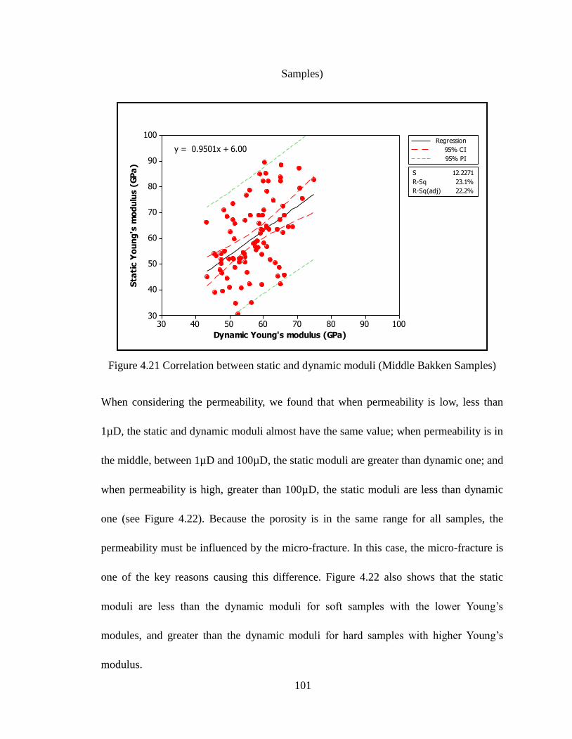
101
Samples)
Figure 4.21 Correlation between static and dynamic moduli (Middle Bakken Samples)
When considering the permeability, we found that when permeability is low, less than
1µD, the static and dynamic moduli almost have the same value; when permeability is in
the middle, between 1µD and 100µD, the static moduli are greater than dynamic one; and
when permeability is high, greater than 100µD, the static moduli are less than dynamic
one (see Figure 4.22). Because the porosity is in the same range for all samples, the
permeability must be influenced by the micro-fracture. In this case, the micro-fracture is
one of the key reasons causing this difference. Figure 4.22 also shows that the static
moduli are less than the dynamic moduli for soft samples with the lower Young’s
modules, and greater than the dynamic moduli for hard samples with higher Young’s
modulus.
10090807060504030
100
90
80
70
60
50
40
30
Dynamic Young's modulus (GPa)
Sta
tic Y
ou
ng
's m
od
ulu
s (
GP
a)
S 12.2271
R-Sq 23.1%
R-Sq(adj) 22.2%
Regression
95% CI
95% PI
y = 0.9501x + 6.00

102
Figure 4.22 Influence of permeability on moduli relationship of static-dynamic
Wang and Nur (2000) proved that the correlations of static and dynamic Young’s
modulus are as follows for soft and hard rocks:
0.41 -1.06static dynamicE E (Static Young’s modulus < 15GPa)
1.153 -15.2static dynamicE E (Static Young’s modulus > 15GPa)
We observe that the dynamic moduli is greater than the static moduli for soft rocks and
some hard rocks, for which the static Young’s modulus is less than 100GPa
approximately; and that the static moduli will be greater than the dynamic one when
static Young’s modulus is over 100GPa.
In this case, the critical value of static Young’s modulus is around 60GPa for our study as

103
comparing to the value of 100GPa for the study of Wang and Nur (2000). As
commented by Mashinsky (2003), the difference between the dynamic and static moduli
of rock comes from the viscoelastic and micro-plastic behavior of the rock, and from the
inelastic mechanisms. Thus when the rock is harder, the plastic behavior of the rock will
be less, this should be the most important factor causing the Estatic and Edynamic
difference for the Bakken samples.
4.4. Compressibility
We did a feasibility study for the proposed methods which use permeability experiment
data to obtain rock compressibility. The lab measurements of 6 cores were used for
verifying Downstream Pressure Build-up method (Table 4.12), and other 9 cores were
measured for verifying Radius-of-Investigation method (Table 4.13). The measure
procedure is exactly the same as the permeability experiment has.
After the compressibility was obtained from the permeability experiment, we compared
the compressibility with the one which was measured directly with the triaxial stress
experiment to evaluate the accuracy of the proposed methods. As shown in Figure 4.23,
and 4.24 for Downstream Pressure Build-up method and Radius-of-Investigation method,
respectively, the compressibilities from the proposed methods are close to those from
triaxial stress experiments. Therefore the proposed methods provide a reliable way to
determine rock compressibility.
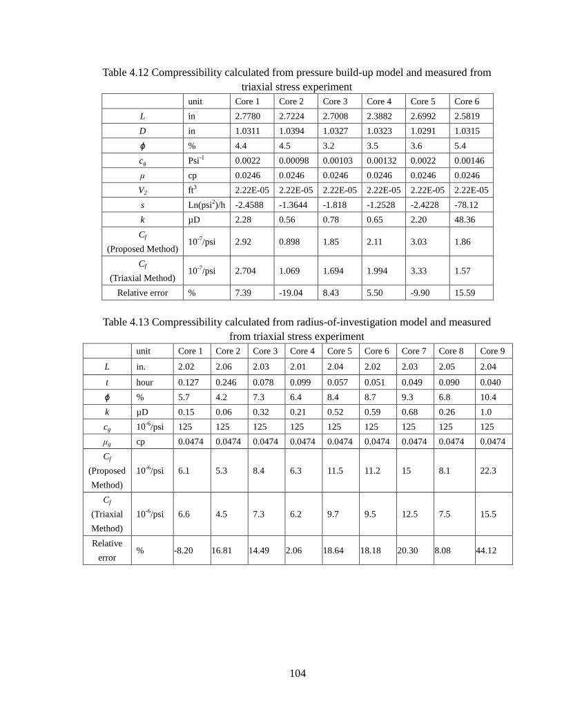
104
Table 4.12 Compressibility calculated from pressure build-up model and measured from
triaxial stress experiment
unit Core 1 Core 2 Core 3 Core 4 Core 5 Core 6
L in 2.7780 2.7224 2.7008 2.3882 2.6992 2.5819
D in 1.0311 1.0394 1.0327 1.0323 1.0291 1.0315
ϕ % 4.4 4.5 3.2 3.5 3.6 5.4
cg Psi-1
0.0022 0.00098 0.00103 0.00132 0.0022 0.00146
μ cp 0.0246 0.0246 0.0246 0.0246 0.0246 0.0246
V2 ft3 2.22E-05 2.22E-05 2.22E-05 2.22E-05 2.22E-05 2.22E-05
s Ln(psi2)/h -2.4588 -1.3644 -1.818 -1.2528 -2.4228 -78.12
k µD 2.28 0.56 0.78 0.65 2.20 48.36
Cf
(Proposed Method) 10
-7/psi 2.92 0.898 1.85 2.11 3.03 1.86
Cf
(Triaxial Method) 10
-7/psi 2.704 1.069 1.694 1.994 3.33 1.57
Relative error % 7.39 -19.04 8.43 5.50 -9.90 15.59
Table 4.13 Compressibility calculated from radius-of-investigation model and measured
from triaxial stress experiment
unit Core 1 Core 2 Core 3 Core 4 Core 5 Core 6 Core 7 Core 8 Core 9
L in. 2.02 2.06 2.03 2.01 2.04 2.02 2.03 2.05 2.04
t hour 0.127 0.246 0.078 0.099 0.057 0.051 0.049 0.090 0.040
ɸ % 5.7 4.2 7.3 6.4 8.4 8.7 9.3 6.8 10.4
k µD 0.15 0.06 0.32 0.21 0.52 0.59 0.68 0.26 1.0
cg 10-6
/psi
125 125 125 125 125 125 125 125 125
μg cp 0.0474 0.0474 0.0474 0.0474 0.0474 0.0474 0.0474 0.0474 0.0474
Cf
(Proposed
Method)
10-6
/psi 6.1 5.3 8.4 6.3 11.5 11.2 15 8.1 22.3
Cf
(Triaxial
Method)
10-6
/psi 6.6 4.5 7.3 6.2 9.7 9.5 12.5 7.5 15.5
Relative
error % -8.20 16.81 14.49 2.06 18.64 18.18 20.30 8.08 44.12

105
Figure 4.23 Comparison of compressibilities calculated by the proposed model
(pressure build-up) and measured by triaxial stress experiment
Figure 4.24 Comparison of compressibilities calculated by the proposed model
(radius-of-investigation) and measured by triaxial stress experiment
The limitation of the Radius-of-Investigation method is the sensitivity of the pressure
gauge needed to be high enough to detect small pressure change. The accuracy of this
method depends on the accuracies of rock porosity, permeability, core length, and gas
0.00000
0.00001
0.00002
0.00003
0.00004
0.00005
0.00006
0 1 2 3 4 5 6 7 8 9 10Core number
Pe
rme
abili
ty (
md
)
-10%
-5%
0%
5%
10%
15%
20%
25%
Re
lati
ve e
rro
r
Compressibility calculated by the proposed model
Compressibility measured by triaxial stress experiment
Relative error

106
compressibility. With a high resolution pressure gauge, a correct capture of pressure
wave arrival can be guaranteed. A good estimation of gas viscosity and permeability at
measured conditions is also important.
The cost to measure rock compressibility can be high and time consuming. The proposed
model provides a way to estimate rock compressibility from permeability experimental
data in case direct compressibility measurement is not available. In the event direct
compressibility measurement is available, the model can serve as a quality control tool.
4.5. Biot’s Coefficient Experimental Result
Table 4.14 shows the result of the Biot's coefficients for 27 Bakken samples using the
proposed method, including 10 vertical direction samples (V-sample, taken perpendicular
to the bedding) and 17 horizontal direction samples (H-sample, taken along the bedding
plane).
Comparing the H-samples to the V-samples in Figure 4.25, we see that the average Biot’s
coefficient of H-sample (0.67) is larger than that of V-sample (0.61). According to
Figures 4.25, 4.26, and 4.27, the Biot’s coefficient of H-sample is higher than that of
V-sample. This anisotropy of Biot’s coefficient of Bakken rock indicates that the Bakken
Formation is heterogeneous. The influence of the pore pressure to the in-situ stress is
greater along the bedding plane than perpendicular to the bedding.
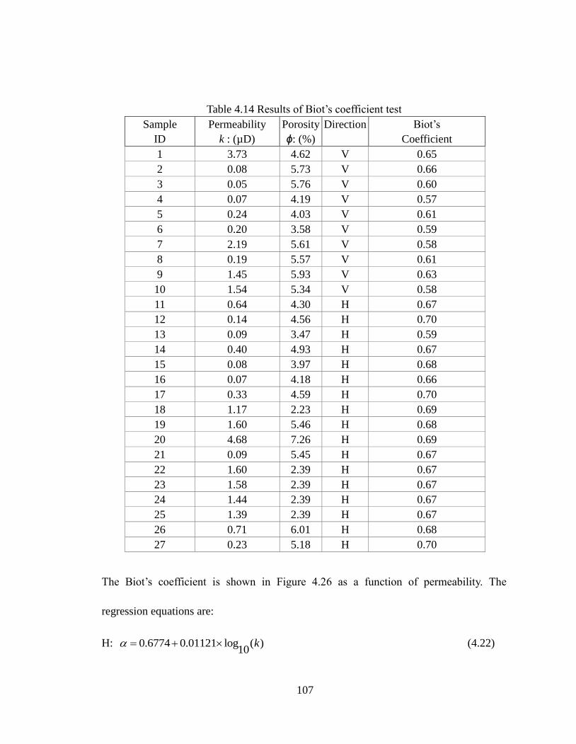
107
Table 4.14 Results of Biot’s coefficient test
Sample
ID
Permeability
k : (µD)
Porosity
ɸ: (%)
Direction Biot’s
Coefficient
1 3.73 4.62 V 0.65
2 0.08 5.73 V 0.66
3 0.05 5.76 V 0.60
4 0.07 4.19 V 0.57
5 0.24 4.03 V 0.61
6 0.20 3.58 V 0.59
7 2.19 5.61 V 0.58
8 0.19 5.57 V 0.61
9 1.45 5.93 V 0.63
10 1.54 5.34 V 0.58
11 0.64 4.30 H 0.67
12 0.14 4.56 H 0.70
13 0.09 3.47 H 0.59
14 0.40 4.93 H 0.67
15 0.08 3.97 H 0.68
16 0.07 4.18 H 0.66
17 0.33 4.59 H 0.70
18 1.17 2.23 H 0.69
19 1.60 5.46 H 0.68
20 4.68 7.26 H 0.69
21 0.09 5.45 H 0.67
22 1.60 2.39 H 0.67
23 1.58 2.39 H 0.67
24 1.44 2.39 H 0.67
25 1.39 2.39 H 0.67
26 0.71 6.01 H 0.68
27 0.23 5.18 H 0.70
The Biot’s coefficient is shown in Figure 4.26 as a function of permeability. The
regression equations are:
H: 0.6774 0.01121 log ( )10
k (4.22)

108
V: 100.6099 0.00523 log ( )k (4.23)
Even though the values of R2 are 6.1% and 1.4% for H-sample regression model and
V-sample regression model, respectively. The Equation 4.22 and Equation 4.23 still
reveal the relations between permeability and Biot’s coefficient.
According to this study (see Figure 4.27), no relationship is found between Biot’s
coefficient and porosity for Bakken Formation.
Figure 4.25 The BoxPlot of Biot’s Coefficient with two groups (horizontal sample and
vertical sample)

109
Figure 4.26 Biot’s coefficient vs. Permeability
Figure 4.27 Biot’s coefficient vs. Porosity

110
4.6. Compressive Strength Experimental Result
We have measured compressive strength for 104 Bakken core plugs from seven wells.
For each individual test, the confining pressure was kept constant in a range from 0 to 20
MPa. Table 4.15 shows the mean compressive strengths at different confining pressures.
The changes of compressive strength caused by confining pressure change are shown
clearly in Figure 4.28.
Table 4.15 Compressive strength in different assessment unit, (MPa)
Assessment Unit Map
Number
Confining Pressure (MPa)
0 5 10 15 20
Nesson-Little Knife
Structural AU
2 133.37 145.03 136.37
96 115.82 120.43 190.17
Central Basin-Poplar
Dome AU 13 131.80 166.10 233.55
Northwest Expulsion
Threshold AU
18 105.80 164.10 181.90
86 101.91 118.87 145.18 169.93
Elm Coulee-Billings
Nose AU 20 130.46 149.52 156.36
Eastern Expulsion
Threshold AU 70 135.91 161.36 165.94

111
Figure 4.28 Mean Compressive Strength vs. Confining Pressure
If the stresses that rocks are subjected to are high enough, then plastic deformation will
be permanent. With plastic deformation, rock cannot be recovered even upon the removal
of the applied stresses. This condition for rock can be caused by three modes: tensile
failure occurs when the effective tensile stress exceeds the tensile strength; compaction
failure occurs under pure hydrostatic loading or non-hydrostatic stress conditions at high
confining pressure; shear failure occurs when the shear stress along some plane is
sufficiently high.
Shear failure is the most common failure mode, which can be described by many
empirical standards. Mohr-Coulomb failure criterion is the most popular one among
those criteria which describe the shear failure. It assumes a linear envelope can be

112
expressed as (Fjaer et al, 1992):
C (4.24)
where τ is the shear strength, µ is the coefficient of internal friction, C is the rock
cohesion, and σ is the normal stress on the shear plane (Figure 4.29).
Figure 4.29 Schematic diagram of Mohr-Coulomb Criterion
σ1: maximum principal stress, σ3: minimum principal stress, and µ = tanɸ.
Based on the ultimate compressive strength, the Mohr-Coulomb failure envelopes are
drawn for the five AUs in Figures E.1, E.2, E.3, E.4 and E.5, respectively. Moreover,
those Mohr-Coulomb failure envelopes are expressed as:
Nesson-Little Knife Structural AU: 0tan(27.8 ) 36.00MPa (4.25)

113
Central Basin-Poplar Dome AU: 0tan(45.17 ) 25.25MPa (4.26)
Northwest Expulsion Threshold AU: 0tan(44.95 ) 20.84MPa (4.27)
Elm Coulee-Billings Nose AU: 0tan(23.37 ) 45.43MPa (4.28)
Eastern Expulsion Threshold AU: 0tan(23.39 ) 48MPa (4.29)
According to the Mohr-Coulomb failure envelopes (Figures E.1 – E.5, and Equations
(4.25) - (4.29)), there exist two classes roughly: one includes Central Basin-Poplar Dome
AU and Northwest Expulsion Threshold AU, which has lower cohesion and higher
coefficient of internal friction; other AUs belong to the second class which has higher
cohesion and lower coefficient of internal friction.

114
CHAPTER V
CONCLUSION AND RECOMMENDATIONS
5.1. Conclusions
Upon the study we finished, following conclusions were made:
1) The freezing sample method is useful to overcome the difficulty of sampling.
2) The porosity of Bakken Formation is usually less than 6%.
3) Three methods to measure the low permeability in the tight rock were proved, and
Radius-of-Investigation method is the fastest one.
4) The compressibility of rock can be obtained indirectly from two permeability
experiments, Downstream Pressure Buil-up measurement and
Radius-of-Investigation measurement.
5) A velocity correlation between P-wave and S-wave derived for Bakken Formation
in this study can be used to estimate the velocity of S-wave from P-wave.
6) The comparison of static and dynamic elastic moduli shows that the static elastic
modulus can be larger than that of dynamic for Bakken Formation.
7) A new method to determine Biot’s Coefficient was proposed.
8) The Biot's coefficients were obtained for Bakken samples which are taken along

115
two principal directions. Horizontal samples lie in the bedding plane, and vertical
samples are perpendicular to the bedding. The average Biot's coefficient for
horizontal samples is 0.67 higher than the one for perpendicular samples. This
anisotropy of Biot’s coefficient of Bakken Formation indicates that the Bakken
Formation is heterogeneous. The influence of the pore pressure to the in-situ
stress is greater along the bedding plane than perpendicular to the bedding.
9) According to the characteristic of Mohr-Coulomb failure envelopes made for the
five AUs (Figure 3.1) with the ultimate compressive strength, there exists two
classes roughly: one includes Central Basin-Poplar Dome AU and Northwest
Expulsion Threshold AU; other AUs belong to the second class.
5.2. Recommendations
Further study focus on:
1) Verifying the permeability measurement with steady-state method.
2) Verifying the result with X-ray microanalysis.
3) Developing effective method to obtain tensile strength of high strength rock, such
as Bakken shale.
4) Combining the core data of this study with well-logs to make a geological model
to better understand Bakken Formation.

116
5) Verifying and using the result in hydraulic fracturing for Bakken Formation to
create more accurate reservoir simulation.

APPENDICES

118
Appendix A
Derivation of Equation for Oscillating Pulse Measurement
Kranz et al. (1990) derived an analytical solution of the diffusion equation for 1-D flow
along a finite sample excited by a pore pressure oscillation. The problem consists on
finding P(x, t) such that
2
2( 0)(0 )
P PD D x L
t x
(A.1)
where D is the coefficient of diffusion, with two boundary conditions:
1) At x=0, (0, ) i tP t Ae ,
2) At x=L, 0( 0)
P P
t x
where ω is the angular frequency, 2g
kA
c V
. k is the permeability, A is the area of
cross-section, V2 is the volume of the downstream reservoir, and µ and cg are the
viscosity and compressibility of the gas, respectively.
The periodic solution as a function of distance x from the upstream and time t is
(1 ) ( ) (1 ) ( )
(1 )NL (1 )NL
{[ (1 ) ] [ (1 ) ] }( , )
[ (1 ) ] [ (1 ) ]
i t i N x L i t i N x L
i i
A i i N e i i N eP x t
i i N e i i N e
(A.2)
where 2N
D
. Thus, at x=L, P(x, t) reduces to:
(1 )NL (1 )NL
[ 2 (1 ) ](L, )
[ (1 ) ] [ (1 ) ]
i t
i i
Ae i NP t
i i N e i i N e
(A.3)
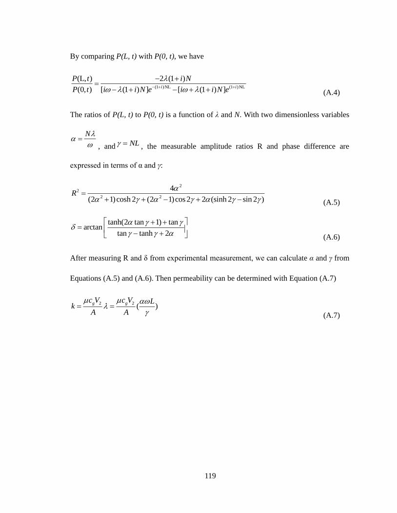
119
By comparing P(L, t) with P(0, t), we have
(1 )NL (1 )NL
(L, ) 2 (1 )
(0, ) [ (1 ) ] [ (1 ) ]i i
P t i N
P t i i N e i i N e
(A.4)
The ratios of P(L, t) to P(0, t) is a function of λ and N. With two dimensionless variables
N
, and NL , the measurable amplitude ratios R and phase difference are
expressed in terms of α and γ:
22
2 2
4
(2 1)cosh 2 (2 1)cos 2 2 (sinh 2 sin 2 )R
(A.5)
tanh(2 tan 1) tanarctan
tan tanh 2
(A.6)
After measuring R and δ from experimental measurement, we can calculate α and γ from
Equations (A.5) and (A.6). Then permeability can be determined with Equation (A.7)
2 2( )
g gc V c V Lk
A A
(A.7)

120
Appendix B
Derivation of Equation for Downstream Pressure Build-up Measurement
Hsieh et al. (1981) and Dicker and Smits (1988) gave the exact solution to Equation
(3.14) for the pressure in the downstream reservoir, which is:
12224
22
21
22
cos][2
00
0
2
m mmm
m
t
abbaabbbaa
babe
abba
b
pmpm
pmtpm
mD
(B.1)
where θm can be calculated from the following equation
ab
)ba(tan
2
(B.2)
where a is the ratio of the sample pore volume (Vp) over the upstream reservoir volume
(V1); and b is the ratio of the sample pore volume over the downstream reservoir volume
(V2),
)V
Vb,
V
Va(
2
p
1
p
.
In Equation (B.1) the dimensionless time, tD, is defined as:
2D
t
ktt
c L
(B.3)
By careful observation it is clear that uz can be treated as a constant in the range of
pressure less than 2000 psi, which is the pressure conditions used in this study. According
to
2( )
b
p
p
pm p dp
z
, the left-hand side (LHS) of Equation (B.1) can be written as
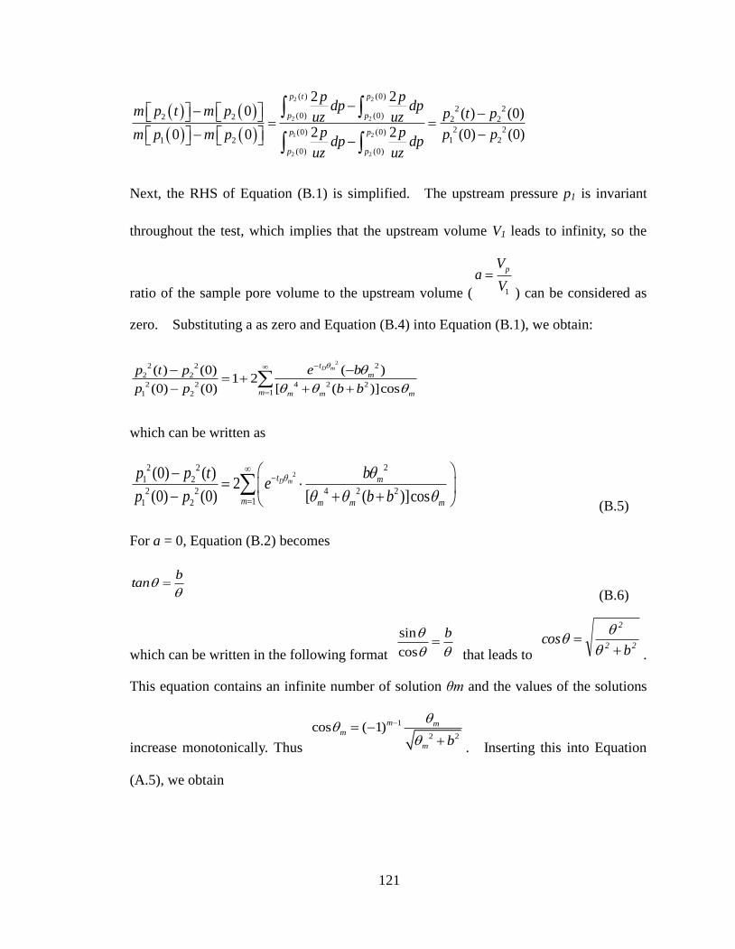
121
(B-4)
Next, the RHS of Equation (B.1) is simplified. The upstream pressure p1 is invariant
throughout the test, which implies that the upstream volume V1 leads to infinity, so the
ratio of the sample pore volume to the upstream volume ( 1
pVa
V
) can be considered as
zero. Substituting a as zero and Equation (B.4) into Equation (B.1), we obtain:
222 2
2 2
2 2 4 2 211 2
( )( ) (0)1 2
(0) (0) [ ( )]cos
D mt
m
m m m m
e bp t p
p p b b
which can be written as
222 2
1 2
2 2 4 2 211 2
(0) ( )2
(0) (0) [ ( )]cosD mt m
m m m m
bp p te
p p b b
(B.5)
For a = 0, Equation (B.2) becomes
btan
(B.6)
which can be written in the following format
sin
cos
b
that leads to 22
2
bcos
.
This equation contains an infinite number of solution θm and the values of the solutions
increase monotonically. Thus
1
2 2cos ( 1)m m
m
m b
. Inserting this into Equation
(A.5), we obtain
2 2
2 2
1 2
2 2
( ) (0)
2 2(0) (0)2 2 2 2
2 2(0) (0)1 21 2
(0) (0)
2 20 ( ) (0)
2 2 (0) (0)0 0
p t p
p p
p p
p p
p pdp dpm p t m p p t puz uz
p p p pm p m pdp dp
uz uz

122
21 4 2 22 2
1 2
2 2 4 2 211 2
( 1)(0) ( )2
(0) (0) ( )D m
m
t m m
m m m
b bp p te
p p b b
(B.7)
Although Dicker and Smits (1988) mentioned that theoretically Equation (B.7) is single
exponentially decreasing only when the upstream reservoir and the downstream reservoir
have the same volume, they still indicated that in order to expedite the experiment in
practical operation the volume of the upstream reservoir is usually much larger than the
volume of the downstream reservoir. In this case, a single exponential equation fit very
well with the downstream pressure build-up curve when the right interval was selected.
Thus, Equation (B.7) was simplified to:
21
4 2 22 21 11 2
2 2 4 2 2
1 2 1 1
(0) ( )2
(0) (0) ( )Dt
b bp p te
p p b b
(B.8)
Letting2 2
1 2( ) (0) ( )p t p p t ,
21
4 2 2
1 1
4 2 2
1 1
( )2
(0) ( )Dt
b bp te
p b b
(B.9)
which can be written as:
21
4 2 2
1 1
4 2 2
1 1
( ) 2 (0)( )
Dtb b
p t p eb b
(B.10)
Taking the natural log of Equation (B.10) yields:

123
4 2 2
1 1 2
14 2 2
1 1
ln ( ) ln 2 (0)( )
D
b bp t p t
b b
(B.11)
Substituting tD from Equation (B.3) into Equation (B.11):
4 2 2 2
1 1 1
4 2 2 2
1 1
ln ( ) ln 2 (0)( ) t
b b kp t p t
b b c L
(B.12)
Figure B.1 ln(∆p) vs. time plot for Core #1.
Assigning
2
1
2
t
ks
c L
, which is the slope of the pressure difference in a logarithm as a
function of time based on Equation (B.12) (Figure B.1); permeability can be easily
obtained from Equation (B.13) when s is fitted as in Figure B.1.
2
2
1
tc Lk s
(B.13)

124
Using the Taylor series of tanθ,
3
tan3
, we can calculate θ1 from Equation (A.6):
1
3
11
b
3
, and
)b3
411(
2
32
1 (B.14)
Substituting Equation (B.14) into Equation (B.13):
22
43 3 1
3
tc L sk
b
(B.15)
Considering that
2
2 2 24
pV AL D Lb
V V V
, the equation becomes:
2
2
2
2
3 3 13
tc L sk
D L
V
(B.16)
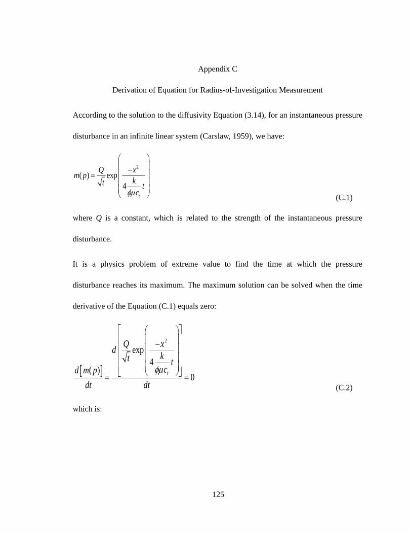
125
Appendix C
Derivation of Equation for Radius-of-Investigation Measurement
According to the solution to the diffusivity Equation (3.14), for an instantaneous pressure
disturbance in an infinite linear system (Carslaw, 1959), we have:
2
( ) exp
4t
Q xm p
kt tc
(C.1)
where Q is a constant, which is related to the strength of the instantaneous pressure
disturbance.
It is a physics problem of extreme value to find the time at which the pressure
disturbance reaches its maximum. The maximum solution can be solved when the time
derivative of the Equation (C.1) equals zero:
2
exp
4( )
0t
Q xd
kt tcd m p
dt dt
(C.2)
which is:

126
2
2
exp
4( )
exp 0
4
t
t
xd
kQ tdcd m p x Qt
kdt dt dtttc
(C.3)
Simplifying the above equations lead to:
3
2
2 2 2
5
2
( )exp exp 0
4 42 4t tt
d m p Q x x Q x
k kdt kt tt tc cc
(C.4)
Finally, Equation (C.5) is obtained as:
3
2
2 2( )exp 1 0
4 22t t
d m p Q x x
k kdtt tt
c c
(C.5)
Considering the initial condition at t=0 and 2( , 0)p x t p , t=0 is a trivial solution to
Equation (C.5). Dividing both sides of the Equation (B.5) by
3
2
2
exp
42t
Q x
ktt
c
yields
2
-1 0
2t
x
kt
c
.
Rearranging the equation, we get the time:

127
2
2
tm
c xt t
k
(C.6)
Expressing permeability in terms of porosity, viscosity, total compressibility, location,
and time, Equation (C.6) can be written as:
2
2
t
m
c xk
t
(C.7)
Converting Equation (C.7) into U.S. field units we have:
21896 t
m
c xk
t
(C.8)
where permeability k is in mD, porosity ɸ is dimensionless (in fraction), viscosity μ is in
cp, total compressibility ct is in psi-1
, time tm is in hour, and location (or distance) x is in
ft.
Equations (C.7) and (C.8) are the governing equations to measure the rock permeability.
They are used to calculate the permeability of any rock that meets the aforementioned
assumptions and can be used for high-permeability rocks as well. The proposed method
evaluates the permeability under unsteady-state flow and requires a short time period to
determine the flow capacity of the low-permeability rock.
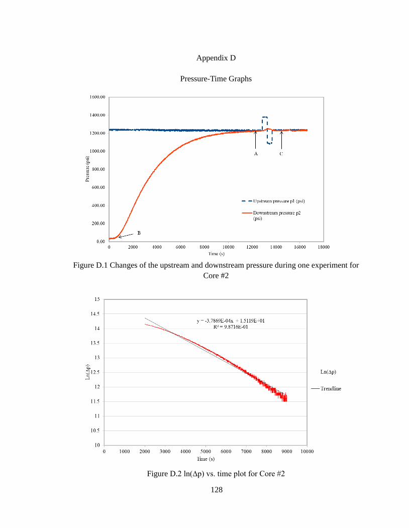
128
Appendix D
Pressure-Time Graphs
Figure D.1 Changes of the upstream and downstream pressure during one experiment for
Core #2
Figure D.2 ln(∆p) vs. time plot for Core #2

129
Figure D.3 Changes of the upstream and downstream pressure during one experiment for
Core #3
Figure D.4 ln(∆p) vs. time plot for Core #3

130
Figure D.5 Changes of the upstream and downstream pressure during one experiment for
Core #4
Figure D.6 ln(∆p) vs. time plot for Core #4

131
Figure D.7 Changes of the upstream and downstream pressure during one experiment for
Core #5
Figure D.8 ln(∆p) vs. time plot for Core #5

132
Figure D.9 Changes of the upstream and downstream pressure during one experiment for
Core #6
Figure D.10 ln(∆p) vs. time plot for Core #6

133
Appendix E
Mohr-Coulomb Failure Envelope
Figure E.1 Mohr-Coulomb failure envelope of Nesson-Little Knife Structural AU
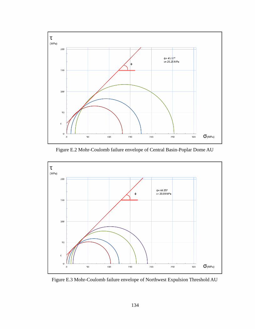
134
Figure E.2 Mohr-Coulomb failure envelope of Central Basin-Poplar Dome AU
Figure E.3 Mohr-Coulomb failure envelope of Northwest Expulsion Threshold AU
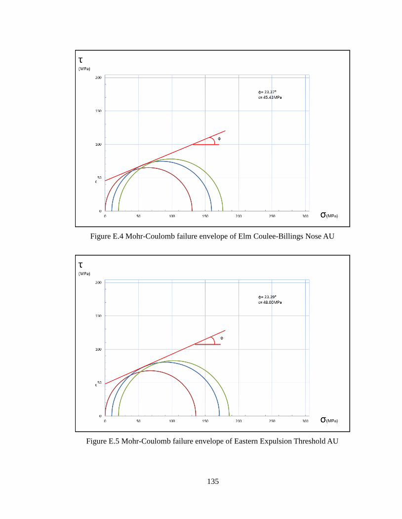
135
Figure E.4 Mohr-Coulomb failure envelope of Elm Coulee-Billings Nose AU
Figure E.5 Mohr-Coulomb failure envelope of Eastern Expulsion Threshold AU
136
REFERENCES
Al-Hussainy, R., Ramey, H. J., & Crawford, P. B. 1966. The Flow of Real Gases Through
Porous Media. Society of Petroleum Engineers.
AutoLab 1500 Manual. 2009. New England Research Inc.
Aviles, C. A., C. H. Scholz, and J. Boatwright. 1987. Fractal analysis applied to
characteristic segments of the San Andreas Fault, J. Geophys. Res., 92(B1), 331–344
Azeemuddin, M., Khan, K., Khan, M. N., Abdulraheem, A., Rahim, Z., & Al-Qahtani, M.
Y. 2002. Experimental Determination of Elastic Anisotropy and Biot's Constant in
a Saudi Arabian Reservoir Sandstone. Society of Petroleum Engineers.
doi:10.2118/78503-MS
Bertoncello, A. and Honarpour, M.M., 2013. Standards for Characterization of Rock
Properties in Unconventional Reservoirs: Fluid Flow Mechanism, Quality Control, and
Uncertainties. SPE 166470-MS
Biot, M. A. 1941. General theory of three-dimensional consolidation, J. appl. Physics,
Lancaster Pa., 12 (1941) 155–164.
Boitnott, G.N., 1997. Use of Complex Pore Pressure Transients to Measure Permeability
of Rocks. SPE 38717-MS
Brace, W. F., and Martin, 1968. A test of the law of effective stress for crystalline rock of
low porosity, International Journal of Rock Mechanics and Mining Science V5 (5)
Brace, W. F., Walsh, J. B., and Frangos, W. T. 1968. Permeability of Granite under High
Pressure. Journal of Geophysical Research, p. 2225-2236.
Bravo, L. and M. Aldana. 2011. Volume curvature attributes to identify subtle faults and
fractures in carbonate reservoirs: Cimarrona Formation, Middle Magdalena Valley Basin,
Colombia. In the 2010 SEG Annual Meeting, Denver, Colorado. 17-22 October, 2010.
Brown, S.R. and C.H. Scholz, 1985. Broad bandwidth study of the topography of natural
rock surfaces. Jour. of Geophys. Res., 90: 12,575 - 12,582.

137
Bruno, M., and Nakagawa, F. M. 1991, Pore pressure influence on tensile fracture
propagation in sedimentary rock V28 (4) (1991) 261–273
Canady, W.J., 2011. A Method for Full-Range Young&apos;s Modulus Correction.
Society of Petroleum Engineers.
Carlaw, H. S., and Jaeger, J. C. 1959. Conduction of Heat in Solids, second edition.
Oxford at Clarendon Press, P50
Carlisle, W.J., Dryff, L., Fryt, M.S., Artindale, J.S., and Von Der Dick, H. 1996. The
Bakken Formation – an Integrated Geologic Approach to Horizontal Drilling. In
Production from Fractured Shales, SPE Reprint Series No. 45, Society of Petroleum
Engineers, Texas.
Carpenter, C.R. and G.R. Spencer. 1940. Measurements of Compressibility of
Consolidated Oil-Bearing Sandstones. Bureau of Mines RI 3540, October 1940.
Cart, J.R. and J.B. Warriner. 1987. Rock mass classification using fractal dimension. In
Proc. 28th U.S. Symp. Rock Mech., I. Farmer, et al., eds., Balkema, Boston, p. 73-80.
Chalaturnyk, R.J. and J.D. Scott. 1992. Evaluation Of Reservoir Properties From
Geomechanical Tests. Journal of Canadian Petroleum Technology. Vol. 31, No. 5, p.
31-40.
Coussy, O. 2005. Poromechanics of freezing materials. Journal of the Mechanics and
Physics of Solids 53: 1689-1718.
Cui, X., Bustin, A.M.M., Bustin, R.M., 2009. Measurements of gas permeability and
diffusivity of tight reservoir rocks: different approaches and their applications. Geofluids
9, P208–223.
Darcy, H. 1856. Les fontaines publiques de la ville de Dijon. Paris: V. Dalmont.
Dennis, B. and E. Slanden. 1988. Fracture Identification Techniques In Carbonates. In
the 39th Annual Technical Meeting of the Petroleum Society of CIM, Calgary, Alberta.
June 12 - 16, 1988.
Dicker, A. I., and Smits, R. M. 1988. A Practical Approach for Determining Permeability
from Laboratory Pressure-Pulse Decay Measurements. SPE 17578, p. 285-292.
Dobrynin, V. M. 1962. Effect of Overburden Pressure on Some Properties Of Sandstones.
Society of Petroleum Engineers. doi:10.2118/461-PA.

138
Dukes, R. T. 2013. Bakken Shale Map - USGS.
http://bakkenshale.com/home/attachment/bakken-formation-map-usgs-2/
Economides, M.J. and Boney, C. 2000. Reservoir Stimulation in Petroleum Production.
In Reservoir Stimulation (Economides and Nolte, eds.), Wiley and Sons, New York.
El-Gezeery, T. M. ., Al-Saqran, F., Archibong, E. I., and Al-Radhi, S. H. 2008. Utilizing
Real Time Logging While Drilling Resistivity Imaging to Identify Fracture Corridors in a
highly fractured Cabonate Reservoir. In the SPE Abu Dhabi International Petroleum
Exhibition and Conference, Abu Dhabi, UAE. 3-6 November, 2008.
Fatt, I. 1953. The Effect of Overburden Pressure on Relative Permeability. Society of
Petroleum Engineers. doi:10.2118/953325-G
Fatt, I. 1958a. Compressibility of sandstones at low to moderate pressures. AAPG
Bulletin, August 1958, Vol. 42, p. 1924-1957.
Fatt, I. 1958b. Pore Volume Compressibilities of Sandstone Reservoir Rocks. Journal of
Petroleum Technology, Vol. 10, No. 3, p. 64-66.
Fatt, I., and Davis, D. H. 1952. Reduction in Permeability With Overburden Pressure.
Society of Petroleum Engineers. doi:10.2118/952329-G
Feng, Q., O. Stephansson, and A. Boberg. 1958. Fracture mapping at exposed rock faces
by using close range digital photogrammetry and geodetic total station. In the 38th U.S.
Symposium on Rock Mechanics (USRMS), Washington, D.C.. 7-10 July, 2001.
Fertl, W. H., and Rieke, H. H. 1980. Gamma Ray Spectral Evaluation Techniques
Identify Fractured Shale Reservoirs and Source-Rock Characteristics. Journal of
Petroleum Technology. Vol. 32, I. 11, p. 2053-2062.
Fischer, D., Smith, S., Peck, W., LeFever, J., LeFever, R., Helms, L., Sorensen, J.,
Steadman, E. and Harju, J. 2005. Overview of Williston Basin geology as it relates to
CO2 sequestration. Report of the Plains CO2 Reduction Partnership Report, 169 Energy
& Environmental Research Center, The University of North Dakota, Grand Forks, North
Dakota.
Fjaer, E., 2008. Petroleum related rock mechanics. Elsevier, Amsterdam; Boston.
Franquet, J. A. S., and Abass, H. H. S. 1999. Experimental evaluation of Biot’s
poroelastic parameterThree different methods. American Rock Mechanics Association.
Geertsma, J. 1957. The Effect of Fluid Pressure Decline on Volumetric Changes of
Porous Rocks. Society of Petroleum Engineers.

139
Greenwald, R.F. and W.H. Somerton. 1981a. Pore Volume Compressibility Data for
Bandera, Berea, and Boise Sandstones, SPE 9746-MS.
Greenwald, R.F. and W.H. Somerton. 1981b. A Theoretical Model For Determination of
Pore Volume Compressibilities of Consolidated Sandstones. SPE 10076-MS, SPE
Annual Technical Conference and Exhibition, 4-7 October 1981, San Antonio, Texas.
Hall, H.N. 1953. Compressibility of Reservoir Rocks. Journal of Petroleum Technology.
Vol. 5, No. 1, p. 17-19.
Han, G. 2011. Natural Fractures in Unconventional Reservoir Rocks: Identification,
Characterization, and its Impact to Engineering Design. In the 45th US Rock
Mechanics/Geomechanics Symposium held in San Francisco, CA, June 26–29, 2011.
Harville, D.W. and Hawkins, M. F. 1969. Rock Compressibility and Failure as Reservoir
Mechanisms in Geopressured Gas Reservoirs. Journal of Petroleum Technology.
Vol. 21, No. 12, p. 1528-1530.
He, J., and Ling, K. 2014. A New Method to Determine Biot Coefficients of Bakken
Samples. American Rock Mechanics Association.
Heck, T.J., LeFever, R.D., Fischer, D.W. and LeFever, J. 2002. Overview of the
Petroleum Geology of the North Dakota Williston Basin. North Dakota Geological
Survey, Bismarck, ND.
Hester, T.C., and Schmoker, J.W. 1985. Selected physical properties of the Bakken
Formation, North Dakota and Montana part of the Williston Basin: U.S. Geological
Survey Oil and Gas Investigations Chart, OC-126, 1 sheet.
Hilbert, L.B.J., Hwong, T.K., Cook, N.G.W., Nihei, K.T., Myer, L.R., 1994. Effects of
Strain Amplitude on the Static and Dynamic Nonlinear Deformation of Berea Sandstone.
1st North American Rock Mechanics Symposium.
Hsieh, P. A., Tracy, J. V., Neuzil, C. E., Bredehoeft, J. D., and Silliman, S. E. 1981. A
transient laboratory method for determining the hydraulic properties of 'tight' rocks-I.
Theory. International Journal of Rock Mechanics and Mining Sciences & Geomechanics
Abstracts, 18, P245-252.
Hu, X., Liang, W., and Hou, S., et al. 2012. Experimental study of effect of temperature
and stress on permeability characteristics of raw coal and shaped coal. Chinese Journal of
Rock Mechanics and Engineering, 31 (6): 1222-1229.

140
Hudson, P.J. and Matson, R.P. 1992. Hydraulic Fracturing in Horizontal Wellbores. Paper
SPE 23950, SPE Permian Basin Oil and Gas Recovery Conference, March 18-20,
Midland, TX.
Hundere, I. 1984. The Effect of Freezing on Unconsolidated Core Ma¬terial from Troll
Field. Internal paper, Saga Petroleum A/S, Oslo.
Ide, J.M., 1936. The elastic properties of rocks: A correlation of theory and experiment.
Proceedings of the National Academy of Sciences of the United States of America 22,
482.
Jaeger, J. Cook, N. G., and Zimmerman, R. 2007. Fundamentals of Rock Mechanics,
4th edition, Malden, MA: Blackwell Pub.
Jones, S. C. 1997. A Technique for Faster Pulse-Decay permeability Measurements in
Tight Rocks. SPE 28450.
K. Terzaghi. 1936. The shearing resistance of saturated soil, Proceeding of the First
International Conference in Soil Mechanics V1 (1936) 54–56.
K. Terzaghi. 1943. Theoretical soil mechanics, J. Wiley & Sons, inc.
Karcher, B. J., Giger, F. M., and Combe, J. 1986. Some Practical Formulas To Predict
Horizontal Well Behavior. Society of Petroleum Engineers. doi:10.2118/15430-MS
Khatchikian, A. 1996. Deriving Reservoir Pore-Volume Compressibility From Well
Logs. SPE Advanced Technology Series. Vol. 4, No. 1, p. 14-20.
Kindt, R.K. 1985. The Effect of Freezing on Permeability of Uncon¬solidated
Sandstones – An Experimental Investigation. Norwegian Institute of Technology,
Trondheim, Norway.
Kranz, R. L., Saltzman, J. S., and Blacic, J. D. 1990. Hydraulic diffusivity measurements
on laboratory rock samples using an oscillating pore pressure method. International
Journal of Rock Mechanics and Mining Sciences & Geomechanics Abstracts 27, p.
345-352.
Labuz, J.F., L.H. Chen, and Cattaneo S. 2001. Fracture of rock from wedge indentation.
In the 38th U.S. Symposium on Rock Mechanics (USRMS), Washington, D.C. 7-10 July,
2001.
Landes, K. 1970. Petroleum Geology of the United States. John Wiley and Sons, New
York.

141
Lantz, T. Greene, D. Eberhard, M., Norrid, S. and Pershall, R. 2007. Refracturing
Treatments
Law, B. E., and Spencer, C. W. 1993. Gas in tight reservoirs-an emerging major source of
energy. The Future of Energy Gasses, US Geological Survey, Professional Paper1570,
P233-252.
Lee, w. J. 1982. Well Testing. SPE Text book Series V1, p.13-15.
LeFever, J. A. 1991. History of oil production from the Bakken Formation, North
Dakota, in, W. B. Hansen, ed., Montana geological Society 1991 Guidebook to Geology
and Horizontal Drilling of the Bakken Formation, Billings, MT, pp. 3-17.
Li, C., X. Chen, and Z. Du. 2004. A New Relationship of Rock Compressibility with
Porosity. SPE 88464-MS, in SPE Asia Pacific Oil and Gas Conference and Exhibition,
Perth, Australia, 18-20 October 2004.
Lin, D., and Fairhurst, C. 1991. The Topological Structure of Fracture Systems In Rock.
American Rock Mechanics Association.
Lin, Q., Labuz, J. F., and Cattaneo, S. 2010. Digital Image Correlation And the Fracture
Process In Rock. American Rock Mechanics Association.
Ling, K. 2012. Correlation between Rock Permeability and Formation Resistivity
Factor-A Rigorous and Theoretical Derivation. In the SPE Middle East Unconventional
Gas Conference and Exhibition. Abu Dhabi, UAE. 23-25 January, 2012.
Locker, D.A. 1993. Acoustic Emission And Rock Fracture. In the 34th U.S. Symposium
on Rock Mechanics (USRMS), Madison, Wisconsin. 28-30 June, 1993.
Look2See1. 2015. Williston Basin. [WWW page]. URL
https://en.wikipedia.org/wiki/Williston_Basin
Macini, P. and E. Mesini. 1998. Static and Dynamic Reservoir Rock Compressibility at
High Pressure. SPE 49549-MS, in SPE Abu Dhabi International Petroleum Exhibition
and Conference, Abu Dhabi, United Arab Emirates, 11-14 November 1998.
Marchina, P., Brousse, A., Fontaine, J., Dano, C., and Alonso, C. 2004. In-situ
Measurement of Rock Compressibility in a Heavy Oil Reservoir. SPE 86940-MS, in SPE
Mashinsky, E.I., 2003. Differences between static and dynamic elastic moduli of rocks:
Physical causes. Differences 44, 953–959.

142
Mavko, G., Mukerji, T., and Dvorkin, J., 2009. The rock physics handbook tools for
seismic analysis of porous media. Cambridge University Press, Cambridge, UK; New
York.
McLatchie, A. S., Hemstock, R. A., and Young, J. W. 1958. The Effective
Compressibility of Reservoir Rock and Its Effects on Permeability. Society of Petroleum
Engineers. doi:10.2118/894-G.
Metwally, Y. M. and Sondergeld, C. H. 2011. Measuring low permeabilities of gas-sands
and shales using a pressure transmission technique. International Journal of Rock
Mechanics & Mining Sciences, p. 1135-1144.
Mukherjee, H., and Economides, M. J. 1991. A Parametric Comparison of Horizontal and
Vertical Well Performance. Society of Petroleum Engineers. doi:10.2118/18303-PA
Neaupane, K., Yamabe, T. and Yoshinaka, R. 1999. Simulation of a fully coupled
thermo-hydro-mechanical system in freezing and thawing rock. International Journal of
Rock Mechanics and Mining Sciences, 36: 563-580.
Nelson, R.A. 1976. An Experimental Study of Fracture Permeability in Porous Rock.
In the 17th U.S. Symposium on Rock Mechanics (USRMS), Snow Bird, Utah. 25-27
August, 1976.
Newman, G.H. 1973. Pore-Volume Compressibility of Consolidated, Friable, and
Unconsolidated Reservoir Rocks Under Hydrostatic Loading. Journal of Petroleum
Technology. Vol. 25, No. 2, p. 129-134.
Nordeng, S.H., 2010, A brief history of oil production from the Bakken Formation in the
Williston Basin: Geo News, v. 37, no. 1, p. 5-9.
Nur, A., and J. D. Byerlee. 1971. An exact effective stress law for elastic deformation of
rock with fluids, J. Geophys. Res., 76(26), 6414–6419
Passey, Q.R., Bohacs, K.M., Esch, W.L., Klimentidis, R., and Sinha, S. 2010. From
Oil-Prone Source Rock to Gas-Producing Shale Reservoir-Geologic and Petrophysical
Characterization of Unconventional Shale-Gas Reservoirs. SPE 131350 presented at the
CPS/SPE International Oil& Gas Conference and Exhibition,
Petrowiki, Compreissibility definition, http://petrowiki.org/Compaction_drive_reservoirs
Plona, T. J. J., and Cook, J. M. J. 1995. Effects of stress cycles on static and dynamic
Young’s moduli in Castlegate sandstone. American Rock Mechanics Association.
Poisson’s Ratio. 2007. http://www.pavementinteractive.org/article/poissons-ratio

143
Pollastro, R. M., T. A. Cook, L. N. R. Roberts, C. J. Schenk, M. D. Lewan, L. O. Anna,
S. B. Gaswirth, P. G. Lillis, T. R. Klett, and R. R. Charpentier, 2008, Assessment of
undiscovered oil resources in the Devonian-Mississippian Bakken Formation, Williston
Basin Province, Montana and North Dakota, 2008: U.S. Geological Survey Fact Sheet
2008-3021, 2 p.
Poston, S.W. and H.Y. Chen. 1987. The Simultaneous Determination of Formation
Compressibility and Gas-in-Place in Abnormally Pressured Reservoirs. SPE 16227, in
SPE Production Operations Symposium, Oklahoma City, Oklahoma, 8-10 March 1987.
Price, L.C. 2000. Origin and Characteristics of the Basin-Centered Continuous-Reservoir
Unconventional Oil-resource Base of Bakken Source System, Williston Basin. Energy
and Environmental research Center
Qiao, L. P., Wong, R. C. K., Aguilera, R., and Kantzas, A. 2012. Determination of Biot's
Effective-Stress Coefficient for Permeability of Nikanassin Sandstone. Society of
Petroleum Engineers. doi:10.2118/150820-PA
Salehi, I. A., & Ciezobka, J. 2013. Controlled Hydraulic Fracturing of Naturally
Fractured Shales - A Case Study in the Marcellus Shale Examining How to Identify and
Exploit Natural Fractures. In the SPE Unconventional Resources Conference-USA, The
Woodlands, Texas, USA. 10-12 April, 2013.
Samson Resources Company. 2006. CMS-300 Conventional Plug Analysis (Corelab
Report, Core Lab File No. Hou-060143). April 24, 2006. In Well File # 16089, Well File
Retrieved from North Dakota Industrial Commission, Oil and Gas Division Database.
https://www.dmr.nd.gov/oilgas/subscriptionservice.asp.
Sanyal, S., Marsden, S. and Ramey, H., 1974. Effect of temperature on petrophysical
properties of reservoir rocks. Paper SPE 4898 presented at the SPE California Regional
Meeting, San Francisco, California, 4-5 April.
Sinha, S., Braun, E.M., Passey, Q.R., Leonardi, S.A., Wood, A.C., Zirkle, T., Boros, J.A.,
and Kudva, R.A. 2012. Advances in Measurement Standards and Flow Properties
Measurements for Tight Rocks such as Shales. SPE 152257-MS, SPE/EAGE European
Unconventional Resources Conference and Exhibition, 20-22 March, Vienna, Austria
Skempton,A W. 1961. Effective stress in soil, concrete and rocks, Pore Pressure and
Suction in Soils (1961) 4–16.
Sloss, L. L. , 1963, Sequences in the cratonic interior of North America: Geological
Society of America Bulletin, v. 74, p. 93-114.

144
Somerton, W.H., Mehta, M.M. and Dean, G.W. 1965. Thermal Alteration of Sandstones.
Journal of Petroleum Technology, May 1965: 589-593.
Sone, H., Zoback, M.D., 2013. Mechanical properties of shale-gas reservoir rocks — Part
1: Static and dynamic elastic properties and anisotropy. GEOPHYSICS 78, D381–D392.
Stanchits S., A. Surdi, E. Edelman, and R. Suarez-Rivera. 2012. Acoustic Emission And
Ultrasonic Transmission Monitoring of Hydraulic Fracture Propagation In
Heterogeneous Rock Samples. In the 46th U.S. Rock Mechanics/Geomechanics
Symposium, Chicago, Illinois. 24-27 June, 2012.
Suman, A. 2009. Uncertainties in Rock Pore Compressibility and Effects on Seismic
History Matching. Master Thesis, Stanford University.
Thorpe, R.K. 1981. An Example Of Fracture Characterization In Granitic Rock. In the
22nd U.S. Symposium on Rock Mechanics (USRMS), Cambridge, Massachusetts. 29
June-2 July, 1981.
Tian, H., Kempka, T. and Schluter, R., et al. 2009. Influence of high temperature on rock
mass surrounding in situ coal conversion sites. Proceedings of the 10th International
Symposium on Environmental Geotechnology and Sustainable Development, Bochum,
Germany, 7-11 September.
Tinni, A., Fathi, E., Agarwal, R., Sondergeld, C., Akkutlu, Y., and Rai, C. 2012. Shale
Permeability Measurements on Plugs and Crushed Samples. SPE 162235, Canadian
Unconventional Resources Conference, 30 October-1 November 2012, Calgary, Alberta,
Canada.
Torsaeter, O. and Beldering, B. 1987. The effect of freezing of slightly consolidated
cores. SPE Formation Evaluation, 2 (3): 357-360. Paper SPE 14300-PA.
Triab, D., and Donaldson, E. C. 2004. Petrophysics (second edition): Theory and Practic
of Measuring Reservoir Rock and Fluid Transport Properties. Amesterdam: Gulf
Professional publishing.
Van der Knaap, W. 1959. Nonlinear Behavior of Elastic Porous Media, Petroleum
Transactions. AIME, Vol. 216, p. 179-187.
Vincent, M.C. 2011. Optimizing Transverse Fractures in Liquid-Rich Formations. SPE
146376, SPE Annual Technical Conference and Exhibition held in Denver, Colorado,
USA, 30 October–2 November 2011
Vodak, F., Trtik, K. and Kapickova, O., et al. 2004. The effect of temperature on strength
– porosity relationship for concrete. Construction and Building Materials, 18: 529-534.
145
Wang, Z. and Nur, A. (eds.), 2000. Seismic and Acoustic Velocities in Reservoir Rocks,
vol. 3,Recent Developments, Geophysics Reprint Series, no. 19. Tulsa, OK: Society of
Exploration Geophysicists.
Yao, T., Li, J. and Huang, Y. 2012. Effects of temperature and stress on porosity and
permeability reservoir. Journal of Shenzhen University Science and Engineering, 29
(2):154-158.
Yildiz, T. 1998. Prediction of In-Situ Formation Compressibility from Production Data,
SPE 47379-MS, in SPE/ISRM Rock Mechanics in Petroleum Engineering, Trondheim,
Norway, 8-10 July 1998.
Yuan, Z., Schubert, J., Teodoriu, C., and Gardoni, P. 2012. HPHT Gas Well Cementing
Complications and its Effect on Casing Collapse Resistance. Paper SPE153986 presented
at the SPE Oil and Gas India Conference and Exhibition, 28-30 March 2012, Mumbai,
India.
Zhou, xuejun. 2011. Geomechanical Stability Analysis for C02 Sequestration in
Carbonate Formation. PhD Dissertation, North Dakota University (May, 2011)
Zimmerman, R. W., W. H. Somerton, and M. S. King. 1986. Compressibility of Porous
Rocks. Journal of Geophysical Research. Vol. 91, No. B12, p. 12765-12777.
Zoback, M. D., and Byerlee, J. D. 1975. Permeability and Effective Stress: GEOLOGIC
NOTES. AAPG Bulletin, 59(1), 154-158.

146
NOMENCLATURE
A : area of the cross section of the core plug
AU : assessment unit
C : constant linear coefficient
C rock cohesion
Cf : formation compressibility
Cg : gas isothermal compressibility
cp : centipoise
Ct : total compressibility
D : Darcy
D : diameter of core
Dcore : core diameter
DOE : U.S. Department of Energy
Edynamic : dynamic Young’s modulus
Estatic : static Young’s modulus
fi,mineral : volumetric fraction of mineral i in total matrix
G : shear modulus
GPa : gigapascal
GRI : Gas Research Institute
: porosity, or original porosity

147
freezer temperature : porosity at freezer temperature
original : original porosity
k : permeability
K : bulk modulus of the rock
Ks : matrix modulus of the rock
L : length of core
Lcore : length of core
M : molecular weight
m(p) : gas pseudopressure
mD : milli-darcy
MPa : megapascal
n : exponential coefficient
n1 : gas moles in Chamber 1
n2 : gas moles in Chamber 2
ND : North Dakota
nD : nano-Darcy
NDIC : North Dakota Industial Commission
OOIP : original oil in place
p : pressure
p1 : initially the pressure in Chamber 1
p1 : upstream reservoir pressure
p1 : pressure at Chamber 1
p2 : initially the pressure in Chamber 2
148
p2 : downstream reservoir pressure
p2 : pressure at Chamber 2
p3 : pressure at Chambers 1 and 2 after pressure reaches equilibrium
pb : base pressure
pc : confining pressure
Pp : pore pressure
P-wave : primary wave
Q : strength of the instantaneous pressure disturbance
qg : gas rate
R : universal gas constant
s : slope of the pressure difference in a logarithm as a function of
time
Sw : water saturation
S-wave : secondary wave
T : temperature
t : time
T1 : temperature at Chamber 1
T2 : temperature at Chamber 2
T3 : temperature at Chambers 1 and 2 after pressure reaches
equilibrium
Tfreezer : freezer temperature
Tfreezing point : water freezing temperature
tm : time at which the pressure disturbance is a maximum at x
UND : University of North Dakota

149
USGS : United States Geological Survey
v : Poisson’s ratio
vdynamic : dynamic Poisson’s ratio
vstatic : Static Poisson's ratio
V1 : volume of the upstream reservoir
V1 : volume of chamber 1 + pipeline volume between Gas Inlet Valve
and Gas Outlet Valve
V2 : volume of the downstream reservoir
V2 : volume of chamber 2 (without core) + pipeline volume between
Gas Outlet Valve and Gas Vent Valve
Vbulk, core : bulk volume of core
Vchamber 1 : volume of chamber 1
Vchamber 2 : volume of chamber 2 (without core)
Vice : ice volume
Voriginal : original volume
Vwater : water volume
Vp : pore volume of the core
Vp : velocity of P-wave
Vs : velocity of S-wave
vx : gas velocity in x direction
x : distance from original point in x direction
z : gas z-factor
z1 : gas z-factor at Chamber 1
z2 : gas z-factor at Chamber 2
150
z3 : gas z-factor at Chambers 1 and 2 after pressure reaches
equilibrium
α : Biot's coefficient
αi,mineral : coefficient of thermal expansion of mineral i
αice : coefficient of thermal expansion of ice
ε : strain
ε1 : first principal normal strain
ε2 : second principal normal strain
ε3 : third principal normal strain
εa : strain of specimen in axial direction
εr : strain of specimen in radial direction
εv : volumetric strain
ρg : gas density
σ : stress
σ΄ : effective stress
σ1 : first principal normal stress
σ2 : second principal normal stress
σ3 : third principal normal stress
τ : shear strength
τm : mean stress
µ : viscosity
µ : coefficient of internal friction
µg : gas viscosity
151
μD : micro-Darcy
Δp : pressure difference
∆pc : Variation of the confining pressure
∆pP : Variation of the pore pressure
∆εv : variation of the volumetric strain
∆σ΄ : variation of the effective stress
Δt : time period
ΔV : variation of the total rock volume
ΔV : volume change
ΔVcontraction, matrix : matrix contraction volume
ΔVcontraction,ice : ice contraction volume
ΔVexpansion : expansion volume due to water phase change
ΔVi,,mineral : mineral i contraction volume
ΔVp : variation of the pore volume
ΔVtotal : total volume change
Δx : incremental distance in x direction