Study of a Shared Autonomous Vehicles Based

Mobility Solution in Stockholm

P i e r r e - J e a n R i g o l e

Master of Science Thesis Stockholm 2014

Pierre-Jean Rigole

Master of Science Thesis STOCKHOLM 2014

STUDY OF A SHARED AUTONOMOUS VEHICLES

BASED MOBILITY SOLUTION IN STOCKHOLM

PRESENTED AT

INDUSTRIAL ECOLOGY ROYAL INSTITUTE OF TECHNOLOGY

Supervisor:

Wilco Burghout Examiner:

Larsgöran Strandberg

TRITA-IM-EX 2014:15 ISSN 1402-7615 Industrial Ecology, Royal Institute of Technology

www.ima.kth.se

I

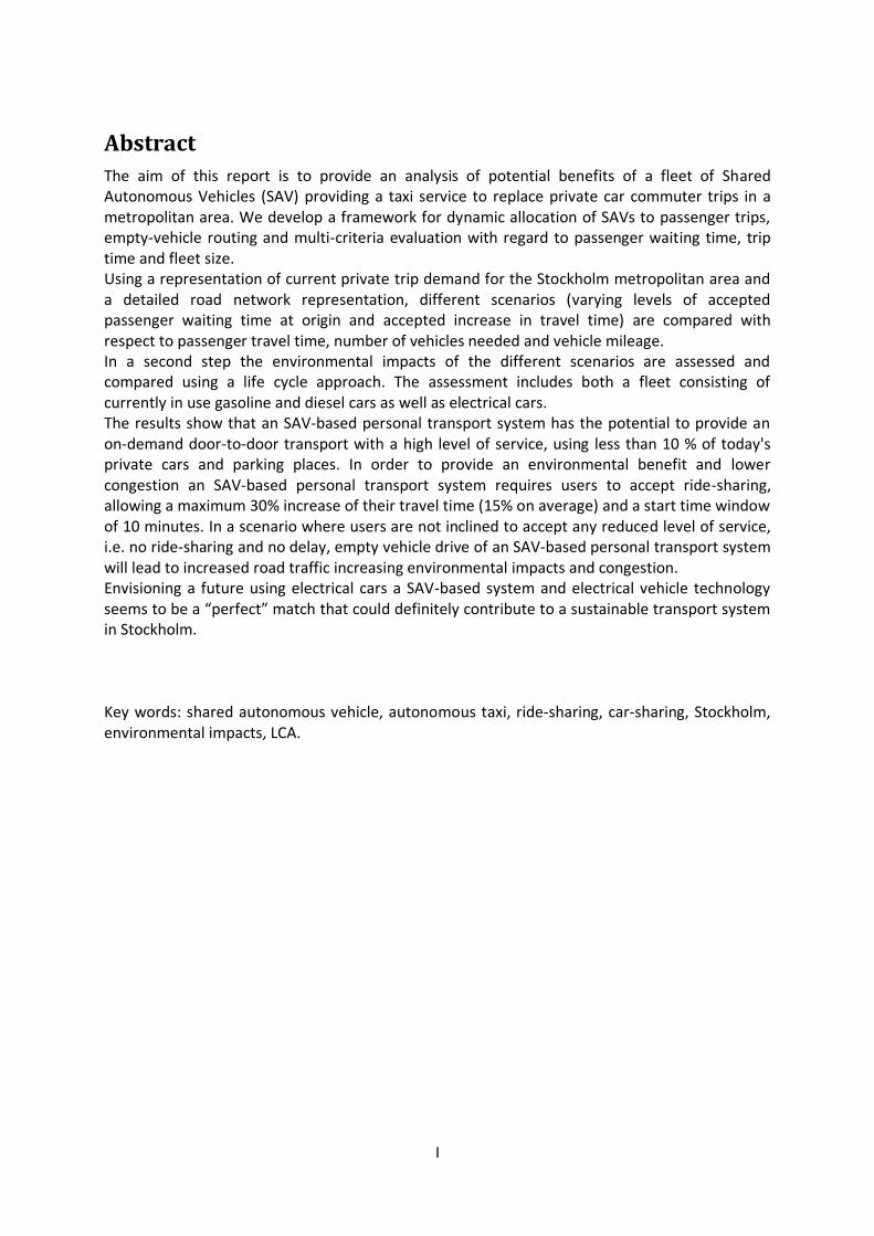
Abstract

The aim of this report is to provide an analysis of potential benefits of a fleet of Shared Autonomous Vehicles (SAV) providing a taxi service to replace private car commuter trips in a metropolitan area. We develop a framework for dynamic allocation of SAVs to passenger trips, empty-vehicle routing and multi-criteria evaluation with regard to passenger waiting time, trip time and fleet size. Using a representation of current private trip demand for the Stockholm metropolitan area and a detailed road network representation, different scenarios (varying levels of accepted passenger waiting time at origin and accepted increase in travel time) are compared with respect to passenger travel time, number of vehicles needed and vehicle mileage. In a second step the environmental impacts of the different scenarios are assessed and compared using a life cycle approach. The assessment includes both a fleet consisting of currently in use gasoline and diesel cars as well as electrical cars. The results show that an SAV-based personal transport system has the potential to provide an on-demand door-to-door transport with a high level of service, using less than 10 % of today's private cars and parking places. In order to provide an environmental benefit and lower congestion an SAV-based personal transport system requires users to accept ride-sharing, allowing a maximum 30% increase of their travel time (15% on average) and a start time window of 10 minutes. In a scenario where users are not inclined to accept any reduced level of service, i.e. no ride-sharing and no delay, empty vehicle drive of an SAV-based personal transport system will lead to increased road traffic increasing environmental impacts and congestion. Envisioning a future using electrical cars a SAV-based system and electrical vehicle technology seems to be a “perfect” match that could definitely contribute to a sustainable transport system in Stockholm. Key words: shared autonomous vehicle, autonomous taxi, ride-sharing, car-sharing, Stockholm, environmental impacts, LCA.

Acknowledgment

I wish to thank various people for their contribution to this project; Wilco Burghout for guiding me into the world of traffic simulation; Ingmar Andreasson and Daniel Jonsson for sharing their expertise and helping in defining the project framework; Kristina Glitterstam for hosting me at Tyréns during my thesis.

III

Table of contents

Abstract .................................................................................................................................. I

Acknowledgment................................................................................................................... II

Table of contents .................................................................................................................. III

1 Introduction .....................................................................................................................1

1.1 Aim and objectives ............................................................................................................ 2

1.2 Scope and limitations ........................................................................................................ 3

1.3 Methodology and Methods .............................................................................................. 3

2 Introduction to self-driving car technology ......................................................................3

3 Modeling of SAV-based system in Stockholm .................................................................5

3.1 System boundaries ............................................................................................................ 6

3.2 Modeling approach ........................................................................................................... 6

3.2.1 Network ..................................................................................................................... 6

3.2.2 Trip demand .............................................................................................................. 8

3.2.3 SAV system modeling .............................................................................................. 11

3.2.4 Ride-sharing ............................................................................................................. 12

3.2.5 SAV assignment - Car-sharing and empty vehicle routing ...................................... 16

3.3 SAV fleet performance indicators ................................................................................... 17

3.4 Simulation results ............................................................................................................ 18

3.4.1 Scenarios.................................................................................................................. 18

3.4.2 Baseline ................................................................................................................... 18

3.4.3 Results for ride-sharing simulation ......................................................................... 19

3.4.4 Results of scenario simulation – SAV fleet performance ........................................ 20

3.4.5 Results of scenario simulation – Environmental impacts ....................................... 22

4 Discussion ..................................................................................................................... 23

5 Conclusion .................................................................................................................... 28

6 References ..................................................................................................................... 29

7 Appendices .................................................................................................................... 33

7.1 Appendix 1 ...................................................................................................................... 33

1

1 Introduction

The invention of the car has shaped our modern society since Karl Benz patented the three-wheeled Motor Car in 1886. Today, it is for many of us the primary mode of transportation and there are currently over 900 million of passenger cars on the road worldwide (World Bank, 2014). While car based mobility system provides considerable personal freedom for those who can afford it and enables substantial economic activity, it is associated with serious side effects in terms of safety, energy, environmental impacts, land use, traffic congestion, time use and equality of access. It is widely acknowledged that today’s car based transport system is unsustainable (Chapman, 2007). In Sweden passenger road transport stands for 16% of the country energy usage and has a large environmental impact resulting from the fossil fuel dependency (Statens energimyndighet, 2013). Therefore, today’s main focus for the transition toward a sustainable transport system in Sweden is to phase out fossil fuel (Regeringskansliet, 2008). This is addressing the environmental impact but does not solve the issue with congestions and safety, which are expected to worsen as urbanization intensifies (World Health Organisation, 2014). In Stockholm traffic is acknowledged as the main environmental issue (Stockholmsstad, 2013) and in 2012 Stockholm was ranked as the eighth most congested city in Europe according to the European traffic index published by the company TomTom (TomTom, 2013). Regarding safety, it is commonly acknowledged that human failure is the dominated cause of car accident, and according to the study performed by Forward (2008) deliberate violations of traffic rules is the main contributor to road crashes. Cars are also utilizing land area not only for roads but also for parking lots. Actually cars are most of the time parked. For instance, in Sweden, based on the average mileage for private cars of 12 000 km per year (Trafikanalys, 2014), the car utilization rate is 4.6%, 2.3% and 1.5% assuming 30, 60 and 90 km/h average speed respectively. This is a consequence of our strong emphasis on individual car ownership, which leads to poor use of precious natural resources and occupy valuable space especially in metropolitan areas. In order to assist drivers various car safety devices have being introduced such as anti-blocking system (ABS), electronic stability control system (ESC) or adaptive cruise control with lane-keep assist. However, with still the driver in charge, these innovations are insufficient in solving the human failure problematic. In this context robotics technology is advocated for critically enhance safety by letting a machine using multiple sensors take the wheel (Thrun, 2010). The horizon for the availability of such vehicles is expected to be 2020-2030 (Nissan, 2013) (Krisher, 2013), with Google leading the field with about 20 self-driving cars which have logged more than 800 000 km on public local streets and highway (Rosenbush, 2013). In Sweden Volvo Car Group together with Trafikverket, Transportstyrelsen, Lindholmen Science Park and Göteborg City started the project Drive Me, a world unique initiative aiming at testing self-driving cars on public roads in Gothenburg (Volvo Car Group, 2013). Self-driving / autonomous cars are promising safer, more comfortable, lower insurance cost and better fuel-efficiency car transport (Marks, 2012) and are expected to solve the congestion issue in urban area (Kornhauser, 2013). They open the possibility to enhance resource utilization by enabling entirely new ride-sharing and car-sharing models (Thrun, 2010) and dramatically cut travel costs (Lawrence D. Burns, 2012), being a crossover between car-sharing programs (such as ZipCar or Car2Go), a taxi service and public transportation. In combination with an efficient

2

public transportation and increase cycling and walking, it could be one of the building blocks of tomorrow’s sustainable transport system, i.e. “a vehicle that improves transportation security and reduces resource depletion and emissions” (Sweeting & Winfield, 2012). So far relatively few studies exist of SAV-based transport systems. Fagnant & Kockelman (2014) use a discrete trip-vehicle allocation model, a theoretical grid network with a synthesized demand based on national travel statistics in the US to simulate the travel and environmental implications of SAVs. However the study does not assume ride-sharing and does not used a real road network. A second paper (Kevin Spieser, 2014) uses an analytical approach to provide guidelines for the design of SAV-based mobility systems, which are applied to the specific case of Singapore to dimension a SAV fleet to serve all ground transport (bus, subway, cars). The advantages of this analytical model are generality and scalability but it does not include ride-sharing nor describes well the inherent discrete and non-linear behavior of traffic. A third article by Kornhauser et al. (2013) assesses the use of a SAV-based (aTaxi) system operating through New Jersey’s roadways, where passengers are loaded and unloaded at dedicated stations available within short walking distance (< 5 min). The model uses a discrete trip-vehicle allocation model and a synthesized demand including 32+ millions of trips made by New Jersey’s 9 million inhabitants, where 90 % is car traffic. The study includes two ride-sharing schemes. (1) ride-sharing with aTaxi waiting a fixed amount of time for additional passengers destined to any destinations that incur less than a 20% detour for any passenger; (2) ride-sharing where the aTaxi sweeps up a local area to pick-up co-passengers with close-by destination and about the same start time. The study provides average vehicle occupancy as function of ride-sharing scheme and waiting time. However it does not include empty vehicle routing, assumes that 14.8% of the trips are served by a combination of railway and SAV, and is not a purely door-to-door service. The study presented in this report investigates potential gains of a fleet of shared autonomous vehicles used as taxi (aTaxis) replacing current private cars for commuting in a metropolitan area, in terms of fleet size, vehicle miles and level of service for passengers. The application focus is the Stockholm metropolitan area, with a dynamic demand representation, ride-sharing and empty-vehicle allocation. The main questions addressed in this paper are: • What is the fleet size needed to serve today's car commuter demand for the Stockholm

metropolitan area, while guaranteeing an acceptable level of service to passengers, in terms of waiting and trip time?

• What is an efficient algorithm to assign trips to a SAV so that passenger level of service and time efficiency is optimized?

• What is an appropriate algorithm to assign empty trips to match supply with demand at origins?

• Do environmental impacts from car traffic improve or worsen?

1.1 Aim and objectives

The study aims at providing an initial assessment of the implementation of a transport service using a fleet of shared autonomous vehicles in Stockholm metropolitan area. The objectives of the study are to: • Introduce autonomous car technology. • Assess potential for a fleet of shared autonomous vehicles (SAV) to serve trip demand

provided today by private cars in Stockholm. Assess number of SAV required, impact on parking requirements, and potential for ride-sharing.

3

• Assess environmental impacts: energy use and emissions of CO2, of a fleet of shared autonomous vehicles (SAV) serving trip demand provided today by private cars in Stockholm.

1.2 Scope and limitations

The implementation of a SAV-based transport system in Stockholm has many aspects related to technology, economy, society and environment. This report touches the technological and environmental parts. It examines the performances of the SAV fleet required to serve the need for personal transportation. This includes calculating the size of the SAV fleet, the mileage, the number of parking places and portion of rides that can be shared by users. Based on these results changes in environmental impacts are assessed and compared relatively to the current state based on data from life cycle assessment for cars. This report does not focus on the technology part although it provides a short presentation of the technology used in autonomous vehicles. The economic and societal aspects are not covered. Furthermore the path for the development of transport system based on driverless car is not investigated. Indeed the design of possible paths requires an interactive process engaging multiple stakeholders, which is not within the scope of this study.

1.3 Methodology and Methods

In this study the scenario methodology is used together with a quantitative assessment of the future state. Methods: This report uses the explorative scenario method, i.e. answering the question: What could happen if an autonomous taxi system is deployed in the city of Stockholm? Different implementations of autonomous taxi are assumed creating several scenarios. The future state is quantitatively assessed using a model for the simulation of the traffic in Stockholm metropolitan area. Key indicators are defined and evaluated, such as the number of cars needed to provide the service, the total mileage travelled, the energy usage or the number of cars parked in the city. These indicators are also evaluated for the current state to provide a baseline for the assessment. Evidence: Researchers at KTH have developed databases to describe travels and passenger behavior in Stockholm (Jonsson, et al., 2011). These data have been validated through previous studies and are used to simulate the implementation of autonomous shared vehicles.

2 Introduction to self-driving car technology

The purpose of this section is to introduce the technology behind self-driving cars which are today already driving on roads. Autonomous car technology shows a tremendous development with Google taking the lead (The Economist, 2014) and there is little doubt that it will mature within the next decade. The main uncertainty might actually not lie in the technology but in its application: will it be used to assist driver to enhance safety as promoted by established car manufacturers or will the technology makes car-sharing the dominant solution for personal mobility? Definitely today’s technology development is driven by the former and has been demonstrated on commercially available vehicles such as Toyota Prius, Lexus RX-450h, Volkswagen Passat, Ford Fusion, Nissan Leaf, or BMW serie 5. The technology can be divided into hardware and software and is described below.

4

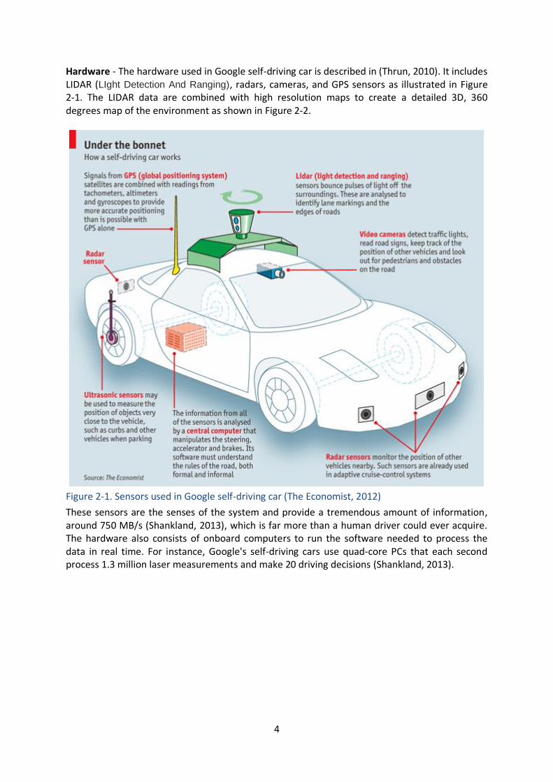
Hardware - The hardware used in Google self-driving car is described in (Thrun, 2010). It includes LIDAR (LIght Detection And Ranging), radars, cameras, and GPS sensors as illustrated in Figure 2-1. The LIDAR data are combined with high resolution maps to create a detailed 3D, 360 degrees map of the environment as shown in Figure 2-2.

Figure 2-1. Sensors used in Google self-driving car (The Economist, 2012)

These sensors are the senses of the system and provide a tremendous amount of information, around 750 MB/s (Shankland, 2013), which is far more than a human driver could ever acquire. The hardware also consists of onboard computers to run the software needed to process the data in real time. For instance, Google's self-driving cars use quad-core PCs that each second process 1.3 million laser measurements and make 20 driving decisions (Shankland, 2013).

5

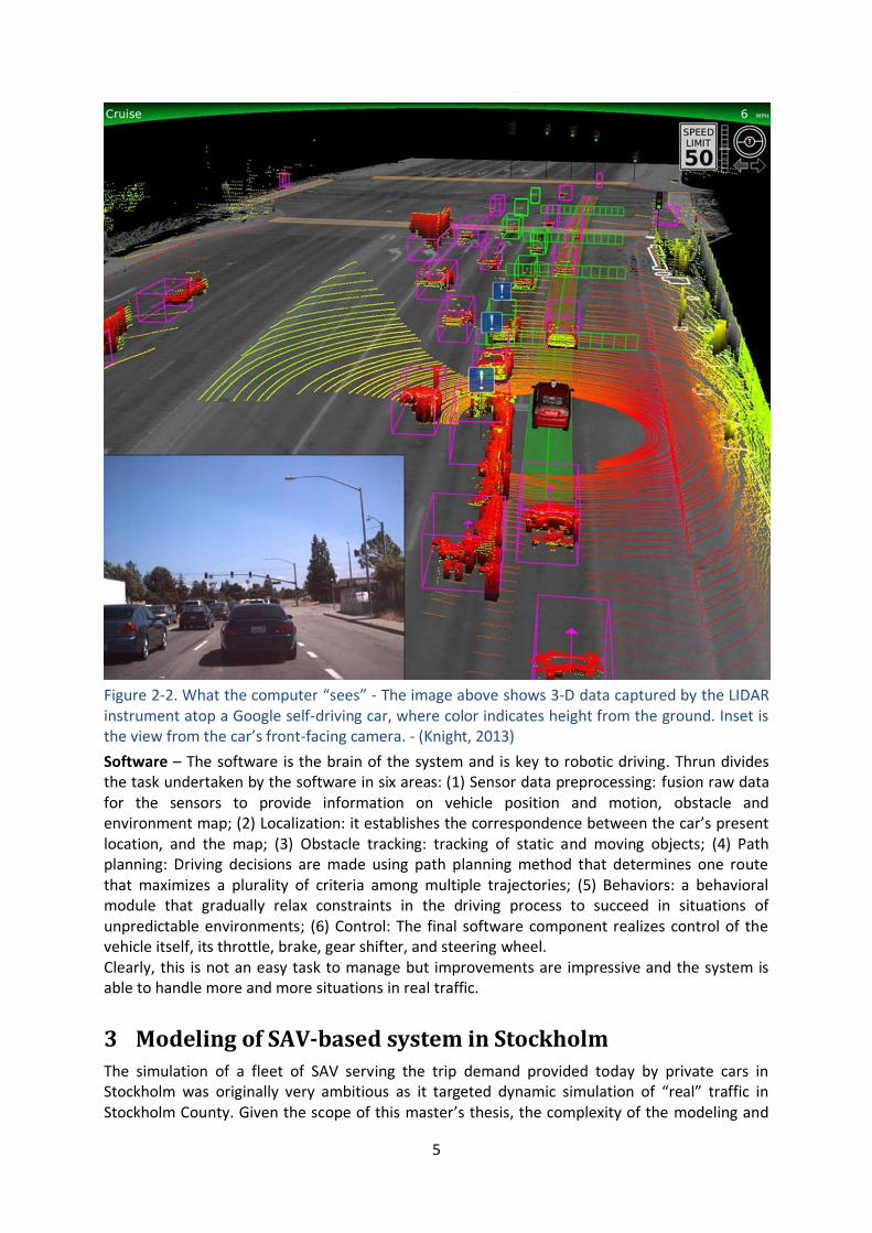
Figure 2-2. What the computer “sees” - The image above shows 3-D data captured by the LIDAR instrument atop a Google self-driving car, where color indicates height from the ground. Inset is the view from the car’s front-facing camera. - (Knight, 2013)

Software – The software is the brain of the system and is key to robotic driving. Thrun divides the task undertaken by the software in six areas: (1) Sensor data preprocessing: fusion raw data for the sensors to provide information on vehicle position and motion, obstacle and environment map; (2) Localization: it establishes the correspondence between the car’s present location, and the map; (3) Obstacle tracking: tracking of static and moving objects; (4) Path planning: Driving decisions are made using path planning method that determines one route that maximizes a plurality of criteria among multiple trajectories; (5) Behaviors: a behavioral module that gradually relax constraints in the driving process to succeed in situations of unpredictable environments; (6) Control: The final software component realizes control of the vehicle itself, its throttle, brake, gear shifter, and steering wheel. Clearly, this is not an easy task to manage but improvements are impressive and the system is able to handle more and more situations in real traffic.

3 Modeling of SAV-based system in Stockholm

The simulation of a fleet of SAV serving the trip demand provided today by private cars in Stockholm was originally very ambitious as it targeted dynamic simulation of “real” traffic in Stockholm County. Given the scope of this master’s thesis, the complexity of the modeling and

6

the limitations in traffic data available the problem definition had to be considerably simplified. In this section, we first present the problem definition, traffic assignment model, traffic data and assumptions used to simulate a transport solution where all private car travels from home to work (H2W) and work to home (W2H) with an origin and a destination within Stockholm metropolitan area are provided by a fleet of SAVs. Then the results of the simulation for different scenarios are presented.

3.1 System boundaries

The geographical border for the study is Stockholm metropolitan area. This delimitation provides a suitable case study. Indeed Stockholm has a dense traffic suitable for SAV implementation, and traffic data and models are available. The time horizon is 2030. This is both long enough to ensure that the technology will be generally available and short enough to still be able to use today traffic data as an acceptable prediction of the traffic situation in Stockholm by 2030.

3.2 Modeling approach

Traffic simulation requires basically the combinations of three elements: (1) a road network; (2) a trip demand; and 3) a trip assignment model. Various combinations of different elements have been evaluated including three road networks for Stockholm metropolitan area, two trip demand sources, and two trip assignment models: Mezzo, a dynamic hybrid microscopic-mesoscopic traffic simulation model (Burghout, 2004), and the development of an own model in MATLAB. In the following, we describe the final model used for the study and shortly explain the rationale for this choice.

3.2.1 Network

A road network consists of nodes/zones that are linked together by a network of roads with crossing including signaling (traffic signals). Each road has a capacity defined by a speed-density function and the number of lanes. Parameters such as resolution, quality of the speed-density function and signaling should be considered when selecting a road networks. In this study three different road networks covering the region Stockholm were considered. These correspond to network coding in three different trip assignment programs: CONTRAM (CONtinuous TRaffic Assignment Model) (Taylor, 2003), EMME/2 (INRO, 2014), and Visum (PTV Group, 2014), and are referred as such. These network codings vary in size and quality. For this study the chosen network is CONTRAM. Indeed, after evaluation, it was deemed to have a suitable size, resolution and signal plan quality for the study. Furthermore it exists a conversion matrix to convert the Regent demand, originally defined in the EMME/2 format, into the CONTRAM format. Another important reason for using the CONTRAM network is that it is already coded in Mezzo, a considerably time consuming task, and hence ready for traffic assignment simulation in Mezzo. The network has been used in several studies related to evaluation of traffic solutions in Stockholm.

3.2.1.1 The CONTRAM network

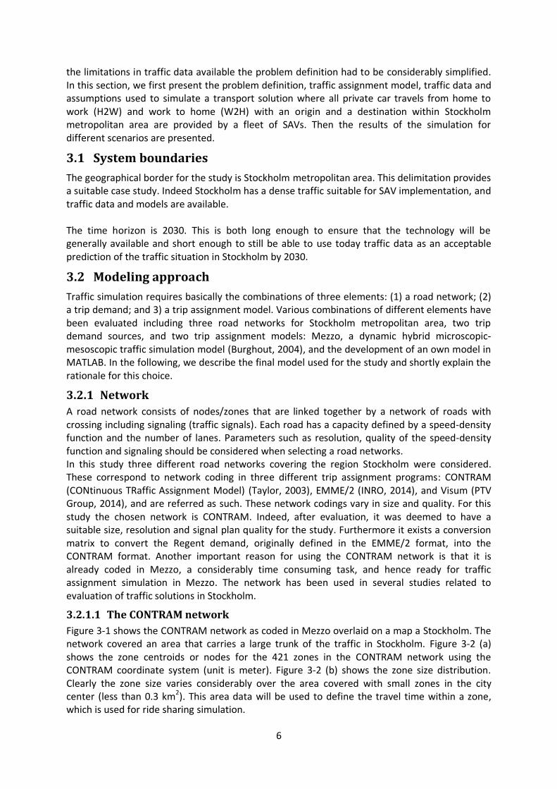
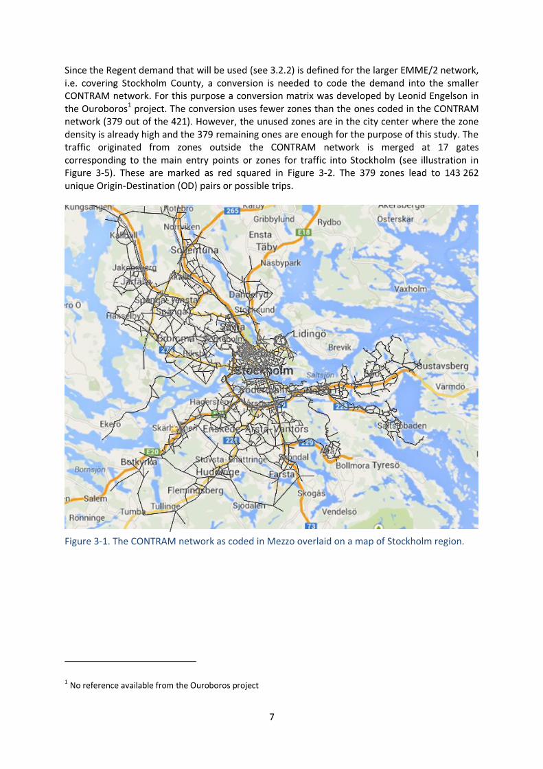
Figure 3-1 shows the CONTRAM network as coded in Mezzo overlaid on a map a Stockholm. The network covered an area that carries a large trunk of the traffic in Stockholm. Figure 3-2 (a) shows the zone centroids or nodes for the 421 zones in the CONTRAM network using the CONTRAM coordinate system (unit is meter). Figure 3-2 (b) shows the zone size distribution. Clearly the zone size varies considerably over the area covered with small zones in the city center (less than 0.3 km2). This area data will be used to define the travel time within a zone, which is used for ride sharing simulation.

7

Since the Regent demand that will be used (see 3.2.2) is defined for the larger EMME/2 network, i.e. covering Stockholm County, a conversion is needed to code the demand into the smaller CONTRAM network. For this purpose a conversion matrix was developed by Leonid Engelson in the Ouroboros1 project. The conversion uses fewer zones than the ones coded in the CONTRAM network (379 out of the 421). However, the unused zones are in the city center where the zone density is already high and the 379 remaining ones are enough for the purpose of this study. The traffic originated from zones outside the CONTRAM network is merged at 17 gates corresponding to the main entry points or zones for traffic into Stockholm (see illustration in Figure 3-5). These are marked as red squared in Figure 3-2. The 379 zones lead to 143 262 unique Origin-Destination (OD) pairs or possible trips.

Figure 3-1. The CONTRAM network as coded in Mezzo overlaid on a map of Stockholm region.

1 No reference available from the Ouroboros project

8

0

20

40

60

80

100

120

140

160

0-29 30-59 60-89 90-119 120-149 150-179 180-209 240-269 270-299 300-330

Fre

qu

en

cy

Time [s]

Intra Zone Driving Time(average speed: 20 km/h)

(a) (b)

Figure 3-2. (a) Zones centroid and gates for the CONTRAM network. (b) Zone size

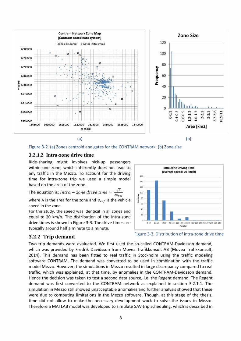
3.2.1.2 Intra-zone drive time

Ride-sharing might involves pick-up passengers within one zone, which inherently does not lead to any traffic in the Mezzo. To account for the driving time for intra-zone trip we used a simple model based on the area of the zone.

The equation is: √

where A is the area for the zone and is the vehicle

speed in the zone. For this study, the speed was identical in all zones and

equal to 20 km/h. The distribution of the intra-zone drive times is shown in Figure 3-3. The drive times are typically around half a minute to a minute.

3.2.2 Trip demand

Two trip demands were evaluated. We first used the so-called CONTRAM-Davidsson demand, which was provided by Fredrik Davidsson from Movea Trafikkonsult AB (Movea Trafikkonsult, 2014). This demand has been fitted to real traffic in Stockholm using the traffic modeling software CONTRAM. The demand was converted to be used in combination with the traffic model Mezzo. However, the simulations in Mezzo resulted in large discrepancy compared to real traffic, which was explained, at that time, by anomalies in the CONTRAM-Davidsson demand. Hence the decision was taken to test a second data source, i.e. the Regent demand. The Regent demand was first converted to the CONTRAM network as explained in section 3.2.1.1. The simulation in Mezzo still showed unacceptable anomalies and further analysis showed that these were due to computing limitations in the Mezzo software. Though, at this stage of the thesis, time did not allow to make the necessary development work to solve the issues in Mezzo. Therefore a MATLAB model was developed to simulate SAV trip scheduling, which is described in

Figure 3-3. Distribution of intra-zone drive time

9

details in section 3.2.3. Without any further evaluation the Regent demand was adopted as it was deemed to be the best alternative.

3.2.2.1 The Regent trip demand

The Regent demand has been synthesized from a survey covering the travelling habits of residents of Stockholm County. The demand described the travels by car from home to work during a normal working day. The data is structured as the number of persons travelling from an origin zone to a destination zone (OD pair). The demand is aggregated, i.e. it provides the total number of travelers for a 24h period without time dependency. Some key features for the demand are summarized in Table 3-1.

Table 3-1. Key features of the Regent trip demand.

Demand Characteristics Regent / Resevanaundersökning (Source: Daniel Jonsson)

Stockholm län

Home-to-work car traffic

Number of trips by OD pair during a normal working day

278 897 trips and 132 976 OD pairs

No time dependency

For this study we assume that all travelers are returning home during the day creating a reverse Work-to-Home (W2H) traffic flow.

3.2.2.2 Timing trip starts

As previously mentioned the Regent demand has no time dependency. For the traffic simulation, the demand needs to be timed, i.e. individual trip need to be distributed over the day. This section describes the procedure to time the Regent demand. The timing of the demand is based on the measurement of the traffic flow at the congestion gates in Stockholm. It assumes that: • The morning and afternoon peaks in the flow measurements are shaped by the H2W and

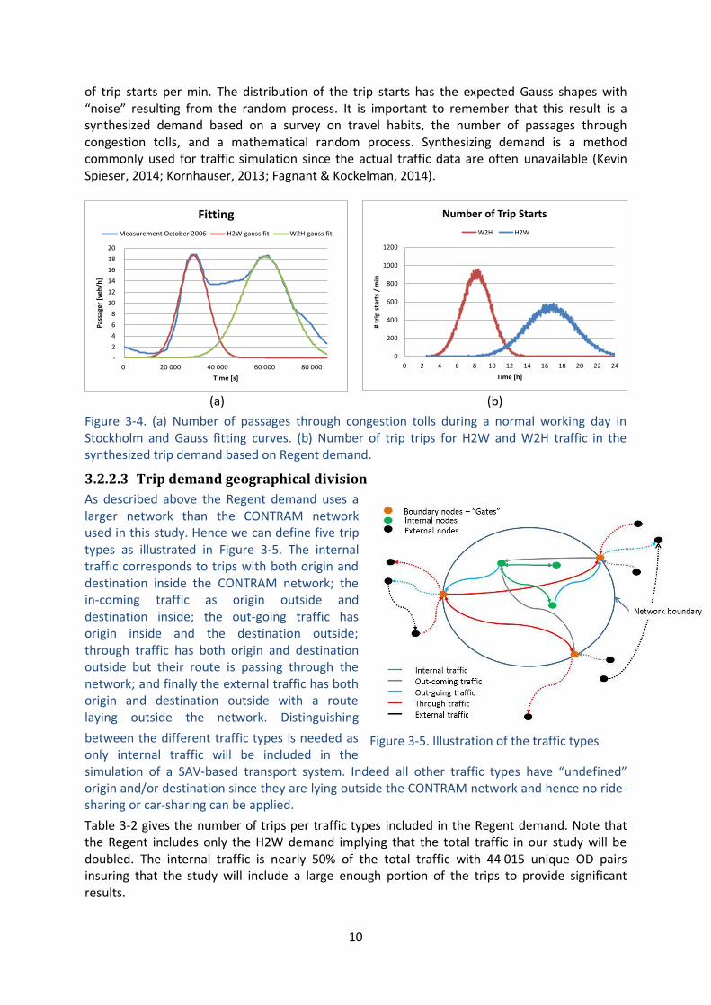
W2H traffic respectively. • The time distribution of the passages is the same as the start time of the trips. • The start time distribution is assumed to have a Gaussian shape. These assumptions imply a non-negligible distortion of the real demand. Indeed the assumption that the start time of trip has the same is distribution as the passage measurement is clearly not true as two cars could have the same passage time but have traveled different distances and hence have different starting times. Another source of distortion is due to the fact that the passage counting registers not only H2W and W2H traffic but also other traffic types not accounted in the Regent demand. Despite its drawbacks this approach was deemed to be “good enough” for the purpose of the study. Figure 3-4 (a) shows the passage measurement taken from (Stockholmsförsöket, 2006) and the two fitting curves to the morning and evening peaks. Of course we need “another” traffic to fill in the gaps outside the rush hours peaks. The two Gauss fitting functions are then used to distribute randomly the trip start time for the H2W and W2H traffic during the day. Intentionally the two functions are set to zero from clock time 00:00 to 1:25 to providing a state when all vehicles in the SAV fleet are assumed to be parked, which is nearly the case in practice as H2W and W2H traffic is very low during this period. The random process is defined by the MATLAB function RAND, which returns a pseudorandom scalar drawn from the standard uniform distribution on the open interval (0,1). The results are presented in Figure 3-4 (b) as the number

10

of trip starts per min. The distribution of the trip starts has the expected Gauss shapes with “noise” resulting from the random process. It is important to remember that this result is a synthesized demand based on a survey on travel habits, the number of passages through congestion tolls, and a mathematical random process. Synthesizing demand is a method commonly used for traffic simulation since the actual traffic data are often unavailable (Kevin Spieser, 2014; Kornhauser, 2013; Fagnant & Kockelman, 2014).

(a) (b)

Figure 3-4. (a) Number of passages through congestion tolls during a normal working day in Stockholm and Gauss fitting curves. (b) Number of trip trips for H2W and W2H traffic in the synthesized trip demand based on Regent demand.

3.2.2.3 Trip demand geographical division

As described above the Regent demand uses a larger network than the CONTRAM network used in this study. Hence we can define five trip types as illustrated in Figure 3-5. The internal traffic corresponds to trips with both origin and destination inside the CONTRAM network; the in-coming traffic as origin outside and destination inside; the out-going traffic has origin inside and the destination outside; through traffic has both origin and destination outside but their route is passing through the network; and finally the external traffic has both origin and destination outside with a route laying outside the network. Distinguishing

between the different traffic types is needed as only internal traffic will be included in the simulation of a SAV-based transport system. Indeed all other traffic types have “undefined” origin and/or destination since they are lying outside the CONTRAM network and hence no ride-sharing or car-sharing can be applied.

Table 3-2 gives the number of trips per traffic types included in the Regent demand. Note that the Regent includes only the H2W demand implying that the total traffic in our study will be doubled. The internal traffic is nearly 50% of the total traffic with 44 015 unique OD pairs insuring that the study will include a large enough portion of the trips to provide significant results.

-

2

4

6

8

10

12

14

16

18

20

0 20 000 40 000 60 000 80 000

Pas

sage

r [v

eh/h

]

Time [s]

Fitting

Measurement October 2006 H2W gauss fit W2H gauss fit

0

200

400

600

800

1000

1200

0 2 4 6 8 10 12 14 16 18 20 22 24#

trip

sta

rts

/ m

inTime [h]

Number of Trip Starts

W2H H2W

Figure 3-5. Illustration of the traffic types

11

Table 3-2. Number of trips per traffic type in the Regent demand for H2W

Traffic type H2W # Vehicles

W2H # Vehicles

% of total

Internal 135 934 135 934 49%

In-coming 68 834 16 856 25%

Out-going 16 856 68 834 6%

Through 6 712 6 712 2%

External 50 561 50 561 18%

3.2.3 SAV system modeling

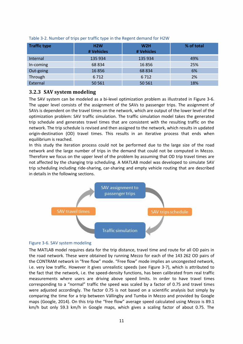
The SAV system can be modeled as a bi-level optimization problem as illustrated in Figure 3-6. The upper level consists of the assignment of the SAVs to passenger trips. The assignment of SAVs is dependent on the travel times on the network, which are output of the lower level of the optimization problem: SAV traffic simulation. The traffic simulation model takes the generated trip schedule and generates travel times that are consistent with the resulting traffic on the network. The trip schedule is revised and then assigned to the network, which results in updated origin-destination (OD) travel times. This results in an iterative process that ends when equilibrium is reached. In this study the iteration process could not be performed due to the large size of the road network and the large number of trips in the demand that could not be computed in Mezzo. Therefore we focus on the upper level of the problem by assuming that OD trip travel times are not affected by the changing trip scheduling. A MATLAB model was developed to simulate SAV trip scheduling including ride-sharing, car-sharing and empty vehicle routing that are described in details in the following sections.

Figure 3-6. SAV system modeling

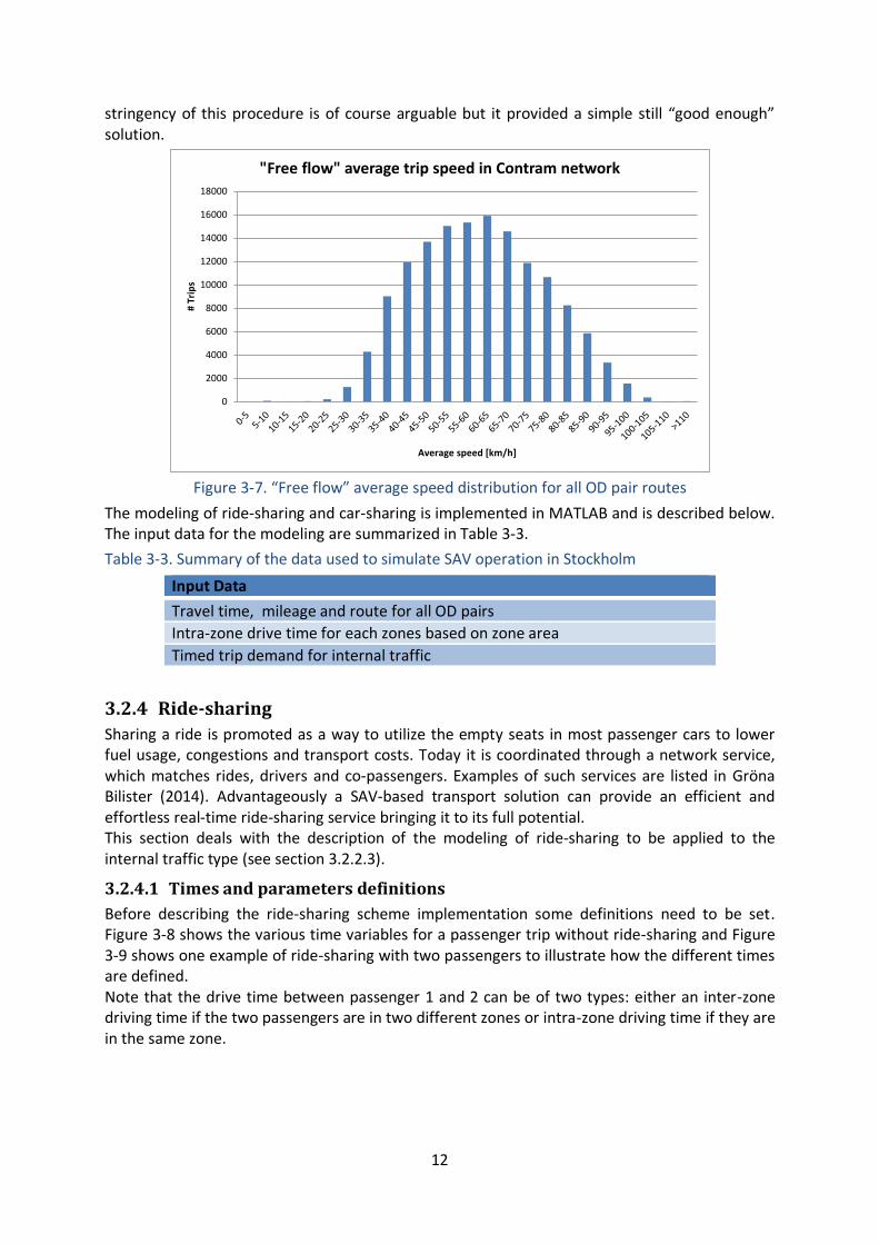
The MATLAB model requires data for the trip distance, travel time and route for all OD pairs in the road network. These were obtained by running Mezzo for each of the 143 262 OD pairs of the CONTRAM network in “free flow” mode. “Free flow” mode implies an uncongested network, i.e. very low traffic. However it gives unrealistic speeds (see Figure 3-7), which is attributed to the fact that the network, i.e. the speed-density functions, has been calibrated from real traffic measurements where users are driving above speed limits. In order to have travel times corresponding to a “normal” traffic the speed was scaled by a factor of 0.75 and travel times were adjusted accordingly. The factor 0.75 is not based on a scientific analysis but simply by comparing the time for a trip between Vällingby and Tumba in Mezzo and provided by Google maps (Google, 2014). On this trip the “free flow” average speed calculated using Mezzo is 89.1 km/h but only 59.3 km/h in Google maps, which gives a scaling factor of about 0.75. The

12

stringency of this procedure is of course arguable but it provided a simple still “good enough” solution.

Figure 3-7. “Free flow” average speed distribution for all OD pair routes

The modeling of ride-sharing and car-sharing is implemented in MATLAB and is described below. The input data for the modeling are summarized in Table 3-3.

Table 3-3. Summary of the data used to simulate SAV operation in Stockholm

Input Data

Travel time, mileage and route for all OD pairs

Intra-zone drive time for each zones based on zone area

Timed trip demand for internal traffic

3.2.4 Ride-sharing

Sharing a ride is promoted as a way to utilize the empty seats in most passenger cars to lower fuel usage, congestions and transport costs. Today it is coordinated through a network service, which matches rides, drivers and co-passengers. Examples of such services are listed in Gröna Bilister (2014). Advantageously a SAV-based transport solution can provide an efficient and effortless real-time ride-sharing service bringing it to its full potential. This section deals with the description of the modeling of ride-sharing to be applied to the internal traffic type (see section 3.2.2.3).

3.2.4.1 Times and parameters definitions

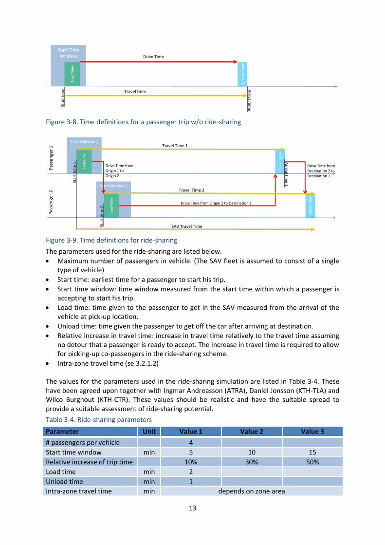
Before describing the ride-sharing scheme implementation some definitions need to be set. Figure 3-8 shows the various time variables for a passenger trip without ride-sharing and Figure 3-9 shows one example of ride-sharing with two passengers to illustrate how the different times are defined. Note that the drive time between passenger 1 and 2 can be of two types: either an inter-zone driving time if the two passengers are in two different zones or intra-zone driving time if they are in the same zone.

0

2000

4000

6000

8000

10000

12000

14000

16000

18000#

Trip

s

Average speed [km/h]

"Free flow" average trip speed in Contram network

13

Figure 3-8. Time definitions for a passenger trip w/o ride-sharing

Figure 3-9. Time definitions for ride-sharing

The parameters used for the ride-sharing are listed below.

Maximum number of passengers in vehicle. (The SAV fleet is assumed to consist of a single type of vehicle)

Start time: earliest time for a passenger to start his trip.

Start time window: time window measured from the start time within which a passenger is accepting to start his trip.

Load time: time given to the passenger to get in the SAV measured from the arrival of the vehicle at pick-up location.

Unload time: time given the passenger to get off the car after arriving at destination.

Relative increase in travel time: increase in travel time relatively to the travel time assuming no detour that a passenger is ready to accept. The increase in travel time is required to allow for picking-up co-passengers in the ride-sharing scheme.

Intra-zone travel time (se 3.2.1.2) The values for the parameters used in the ride-sharing simulation are listed in Table 3-4. These have been agreed upon together with Ingmar Andreasson (ATRA), Daniel Jonsson (KTH-TLA) and Wilco Burghout (KTH-CTR). These values should be realistic and have the suitable spread to provide a suitable assessment of ride-sharing potential.

Table 3-4. Ride-sharing parameters

Parameter Unit Value 1 Value 2 Value 3

# passengers per vehicle 4

Start time window min 5 10 15

Relative increase of trip time 10% 30% 50%

Load time min 2

Unload time min 1

Intra-zone travel time min depends on zone area

Start Time Window

Load

Tim

e

Star

t ti

me

Drive Time

Arrival tim

e

Un

load

Tim

e

Travel time

Start Window 1

Load

Tim

e

Start Window 2

Un

load

Tim

e

Load

Tim

e

Un

load

Tim

e

SAV Travel Time

Star

t ti

me

1 A

rrival time 1

St

art

tim

e 2

Drive Time from Origin 2 to Destination 1

Drive Time from Destination 2 to Destination 1

Drive Time from Origin 1 to Origin 2

Travel Time 2

Travel Time 1

Pass

enge

r 1

Pass

en

ger

2

14

The maximum number of passengers per vehicle is set to four. This is not only a practical value since most of today’s personal cars are designed for four passengers, it is also large enough for not being a significant limitation factor for ride-sharing, i.e. only few rides can be shared by more than four passengers. To support this statement one can compute a higher bound for the number of possible co-passengers for each trip assuming no detour to pick-up passenger. The number of passengers is then given by:

Analyzing the demand in the case of 50% relative increase of trip time, 2 min and 1 min load and unload time, and a fixed 1 min intra-zone travel time, the number of trips with potentially more than four passengers is only 15%. Remembering that this is an upper bound, which assumes an unrealistic case. The actual number should be significantly lower.

3.2.4.2 Rules for ride-sharing

The following general rules apply to the ride-sharing scheme implemented in this study. 1. Within a destination zone unloading passengers is done in the same order as they were

loaded. 2. If several itineraries are possible, i.e. the SAV has different co-passenger alternatives

implying different routes/itineraries, then the itinerary with the shortest drive time for the SAV is chosen.

3. If several co-passengers are possile for a given itinerary then the one with the closest start time is chosen.

4. Unload time is assumed to shorter than load time.

3.2.4.3 Ride-sharing schemes

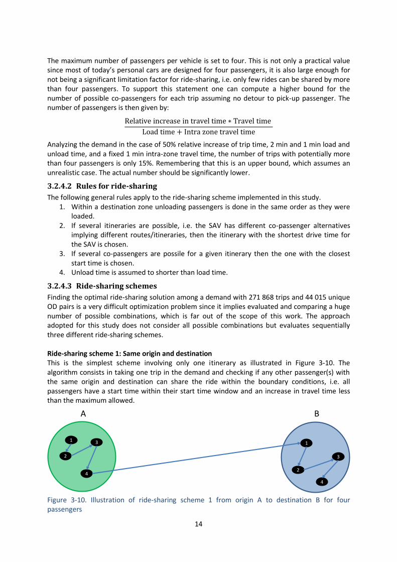
Finding the optimal ride-sharing solution among a demand with 271 868 trips and 44 015 unique OD pairs is a very difficult optimization problem since it implies evaluated and comparing a huge number of possible combinations, which is far out of the scope of this work. The approach adopted for this study does not consider all possible combinations but evaluates sequentially three different ride-sharing schemes. Ride-sharing scheme 1: Same origin and destination This is the simplest scheme involving only one itinerary as illustrated in Figure 3-10. The algorithm consists in taking one trip in the demand and checking if any other passenger(s) with the same origin and destination can share the ride within the boundary conditions, i.e. all passengers have a start time within their start time window and an increase in travel time less than the maximum allowed.

Figure 3-10. Illustration of ride-sharing scheme 1 from origin A to destination B for four passengers

A B

1

2

3

4

1

2

3

4

15

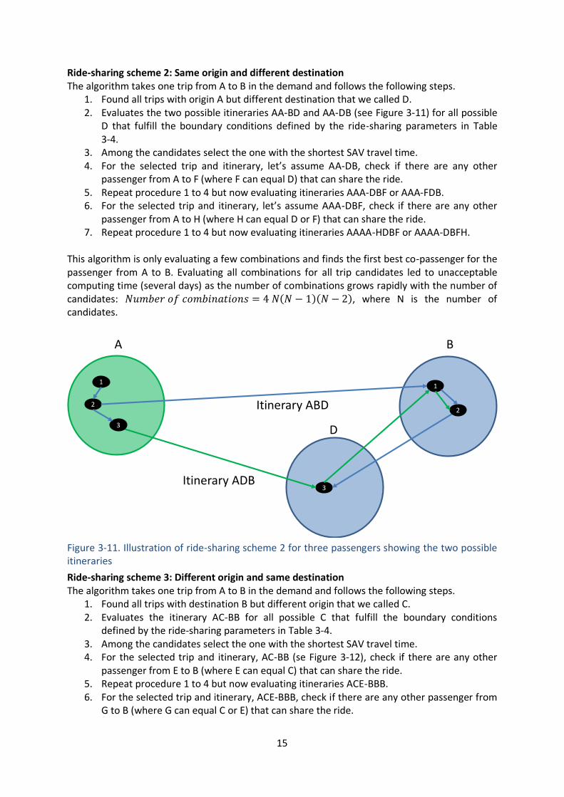
Ride-sharing scheme 2: Same origin and different destination The algorithm takes one trip from A to B in the demand and follows the following steps.

1. Found all trips with origin A but different destination that we called D. 2. Evaluates the two possible itineraries AA-BD and AA-DB (see Figure 3-11) for all possible

D that fulfill the boundary conditions defined by the ride-sharing parameters in Table 3-4.

3. Among the candidates select the one with the shortest SAV travel time. 4. For the selected trip and itinerary, let’s assume AA-DB, check if there are any other

passenger from A to F (where F can equal D) that can share the ride. 5. Repeat procedure 1 to 4 but now evaluating itineraries AAA-DBF or AAA-FDB. 6. For the selected trip and itinerary, let’s assume AAA-DBF, check if there are any other

passenger from A to H (where H can equal D or F) that can share the ride. 7. Repeat procedure 1 to 4 but now evaluating itineraries AAAA-HDBF or AAAA-DBFH.

This algorithm is only evaluating a few combinations and finds the first best co-passenger for the passenger from A to B. Evaluating all combinations for all trip candidates led to unacceptable computing time (several days) as the number of combinations grows rapidly with the number of candidates: ( )( ), where N is the number of candidates.

Figure 3-11. Illustration of ride-sharing scheme 2 for three passengers showing the two possible itineraries

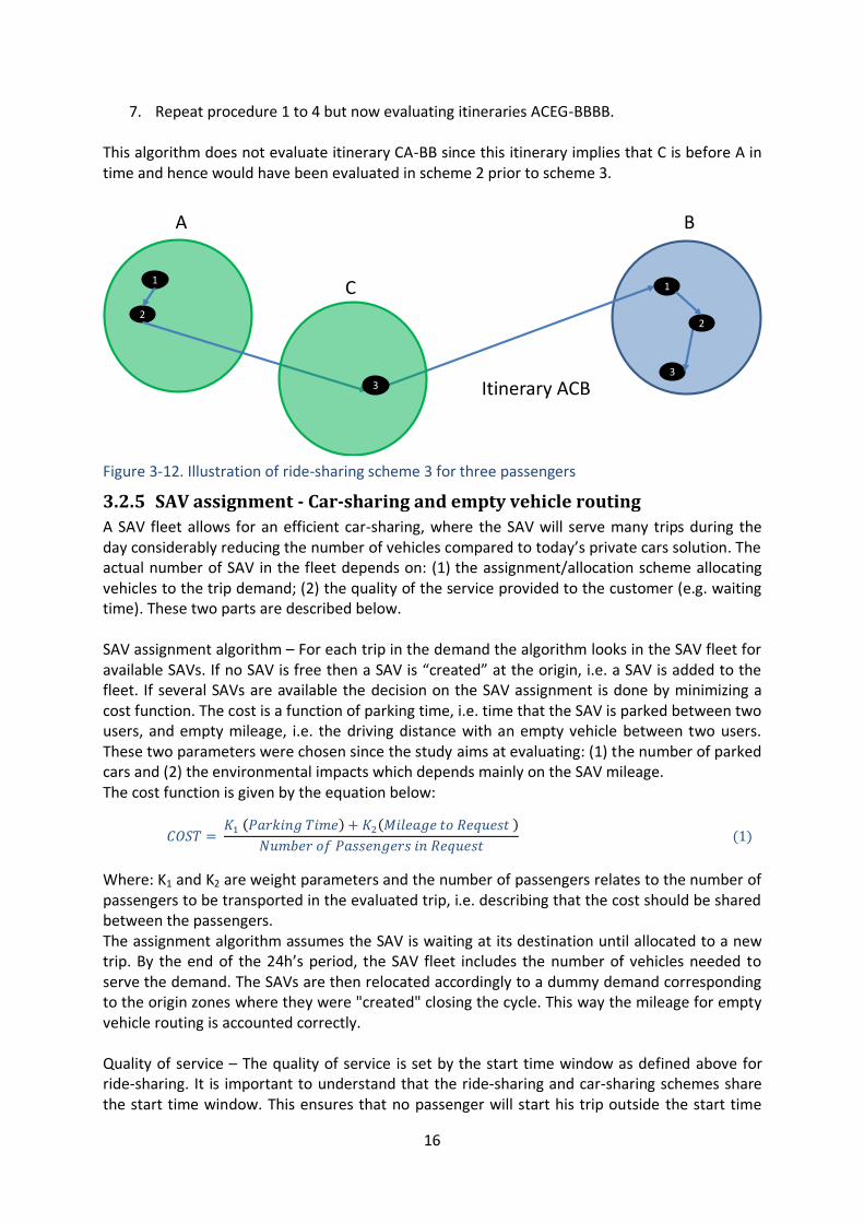
Ride-sharing scheme 3: Different origin and same destination The algorithm takes one trip from A to B in the demand and follows the following steps.

1. Found all trips with destination B but different origin that we called C. 2. Evaluates the itinerary AC-BB for all possible C that fulfill the boundary conditions

defined by the ride-sharing parameters in Table 3-4. 3. Among the candidates select the one with the shortest SAV travel time. 4. For the selected trip and itinerary, AC-BB (se Figure 3-12), check if there are any other

passenger from E to B (where E can equal C) that can share the ride. 5. Repeat procedure 1 to 4 but now evaluating itineraries ACE-BBB. 6. For the selected trip and itinerary, ACE-BBB, check if there are any other passenger from

G to B (where G can equal C or E) that can share the ride.

A B

1

2

1

3

D

Itinerary ABD

Itinerary ADB

3

2

16

7. Repeat procedure 1 to 4 but now evaluating itineraries ACEG-BBBB. This algorithm does not evaluate itinerary CA-BB since this itinerary implies that C is before A in time and hence would have been evaluated in scheme 2 prior to scheme 3.

Figure 3-12. Illustration of ride-sharing scheme 3 for three passengers

3.2.5 SAV assignment - Car-sharing and empty vehicle routing

A SAV fleet allows for an efficient car-sharing, where the SAV will serve many trips during the day considerably reducing the number of vehicles compared to today’s private cars solution. The actual number of SAV in the fleet depends on: (1) the assignment/allocation scheme allocating vehicles to the trip demand; (2) the quality of the service provided to the customer (e.g. waiting time). These two parts are described below. SAV assignment algorithm – For each trip in the demand the algorithm looks in the SAV fleet for available SAVs. If no SAV is free then a SAV is “created” at the origin, i.e. a SAV is added to the fleet. If several SAVs are available the decision on the SAV assignment is done by minimizing a cost function. The cost is a function of parking time, i.e. time that the SAV is parked between two users, and empty mileage, i.e. the driving distance with an empty vehicle between two users. These two parameters were chosen since the study aims at evaluating: (1) the number of parked cars and (2) the environmental impacts which depends mainly on the SAV mileage. The cost function is given by the equation below:

( ) ( )

( )

Where: K1 and K2 are weight parameters and the number of passengers relates to the number of passengers to be transported in the evaluated trip, i.e. describing that the cost should be shared between the passengers. The assignment algorithm assumes the SAV is waiting at its destination until allocated to a new trip. By the end of the 24h’s period, the SAV fleet includes the number of vehicles needed to serve the demand. The SAVs are then relocated accordingly to a dummy demand corresponding to the origin zones where they were "created" closing the cycle. This way the mileage for empty vehicle routing is accounted correctly. Quality of service – The quality of service is set by the start time window as defined above for ride-sharing. It is important to understand that the ride-sharing and car-sharing schemes share the start time window. This ensures that no passenger will start his trip outside the start time

A B

1

2

1

3

Itinerary ACB

2

C

3

17

window when both the ride- and car-sharing schemes are applied. Note that, since we apply ride-sharing first, the car-sharing scheme is utilizing the remaining part of start time window. For instance, if a passenger has a start time of 8:00 and the start time window is 10 min, then he can have an actual start time up to 8:10 where the 10 min shift could be partly due to ride-sharing (i.e. matching its trip to co-passenger(s)) and partly due to car-sharing, i.e. time for an SAV to drive from his latest destination to the new customer. The car-sharing algorithm follows the following steps:

1. Take one request for a trip/SAV and check which SAVs are free or will be free in time to serve the request.

2. If the number of candidates is zero then “create” a SAV and take next request. 3. If the number of candidates is larger than one then choose the one with the lowest cost

function. 4. At the end of the 24h’s period relocate SAVs to the zones where they were once

“created” choosing the nearest zone from their current position.

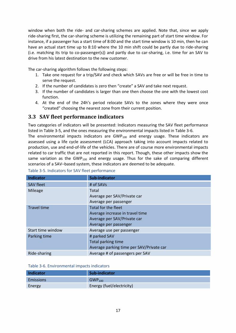
3.3 SAV fleet performance indicators

Two categories of indicators will be presented: Indicators measuring the SAV fleet performance listed in Table 3-5, and the ones measuring the environmental impacts listed in Table 3-6. The environmental impacts indicators are GWP100 and energy usage. These indicators are assessed using a life cycle assessment (LCA) approach taking into account impacts related to production, use and end-of-life of the vehicles. There are of course more environmental impacts related to car traffic that are not reported in this report. Though, these other impacts show the same variation as the GWP100 and energy usage. Thus for the sake of comparing different scenarios of a SAV–based system, these indicators are deemed to be adequate.

Table 3-5. Indicators for SAV fleet performance

Indicator Sub-indicator

SAV fleet # of SAVs

Mileage Total Average per SAV/Private car Average per passenger

Travel time Total for the fleet Average increase in travel time Average per SAV/Private car Average per passenger

Start time window Average use per passenger

Parking time # parked SAV Total parking time Average parking time per SAV/Private car

Ride-sharing Average # of passengers per SAV

Table 3-6. Environmental impacts indicators

Indicator Sub-indicator

Emissions GWP100

Energy Energy (fuel/electricity)

18

3.4 Simulation results

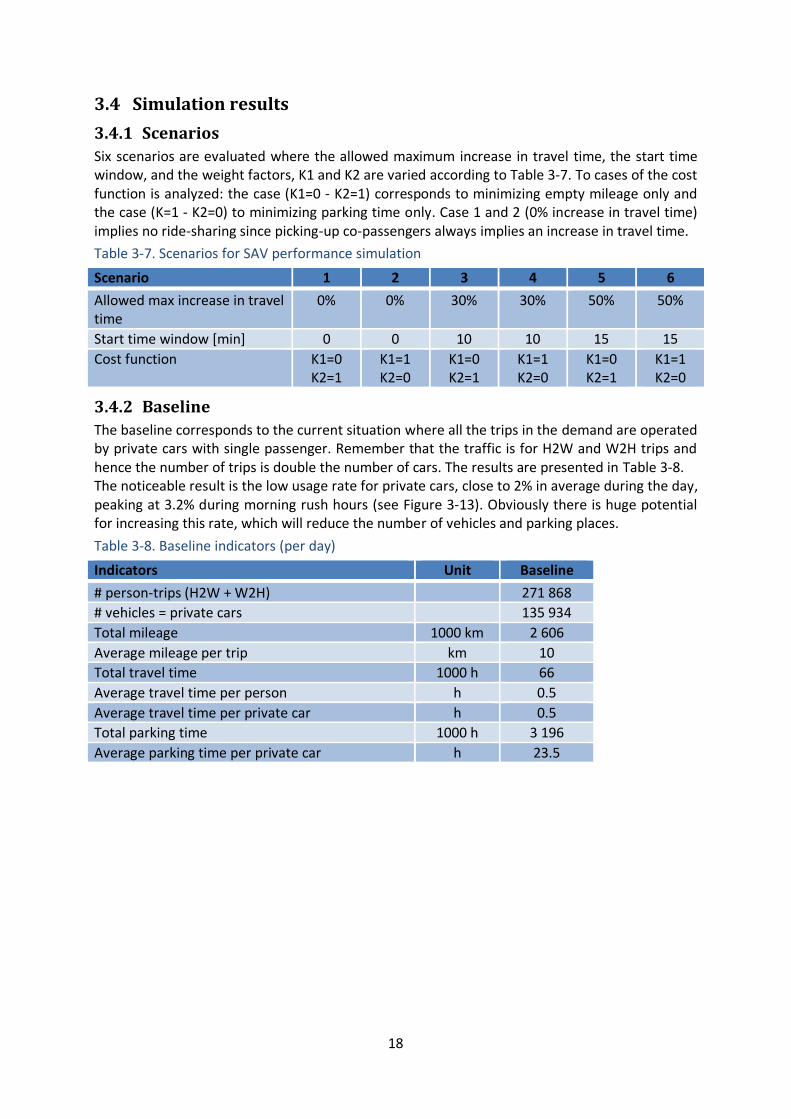
3.4.1 Scenarios

Six scenarios are evaluated where the allowed maximum increase in travel time, the start time window, and the weight factors, K1 and K2 are varied according to Table 3-7. To cases of the cost function is analyzed: the case (K1=0 - K2=1) corresponds to minimizing empty mileage only and the case (K=1 - K2=0) to minimizing parking time only. Case 1 and 2 (0% increase in travel time) implies no ride-sharing since picking-up co-passengers always implies an increase in travel time.

Table 3-7. Scenarios for SAV performance simulation

Scenario 1 2 3 4 5 6

Allowed max increase in travel time

0% 0% 30% 30% 50% 50%

Start time window [min] 0 0 10 10 15 15

Cost function K1=0 K2=1

K1=1 K2=0

K1=0 K2=1

K1=1 K2=0

K1=0 K2=1

K1=1 K2=0

3.4.2 Baseline

The baseline corresponds to the current situation where all the trips in the demand are operated by private cars with single passenger. Remember that the traffic is for H2W and W2H trips and hence the number of trips is double the number of cars. The results are presented in Table 3-8. The noticeable result is the low usage rate for private cars, close to 2% in average during the day, peaking at 3.2% during morning rush hours (see Figure 3-13). Obviously there is huge potential for increasing this rate, which will reduce the number of vehicles and parking places.

Table 3-8. Baseline indicators (per day)

Indicators Unit Baseline

# person-trips (H2W + W2H) 271 868

# vehicles = private cars 135 934

Total mileage 1000 km 2 606

Average mileage per trip km 10

Total travel time 1000 h 66

Average travel time per person h 0.5

Average travel time per private car h 0.5

Total parking time 1000 h 3 196

Average parking time per private car h 23.5

19

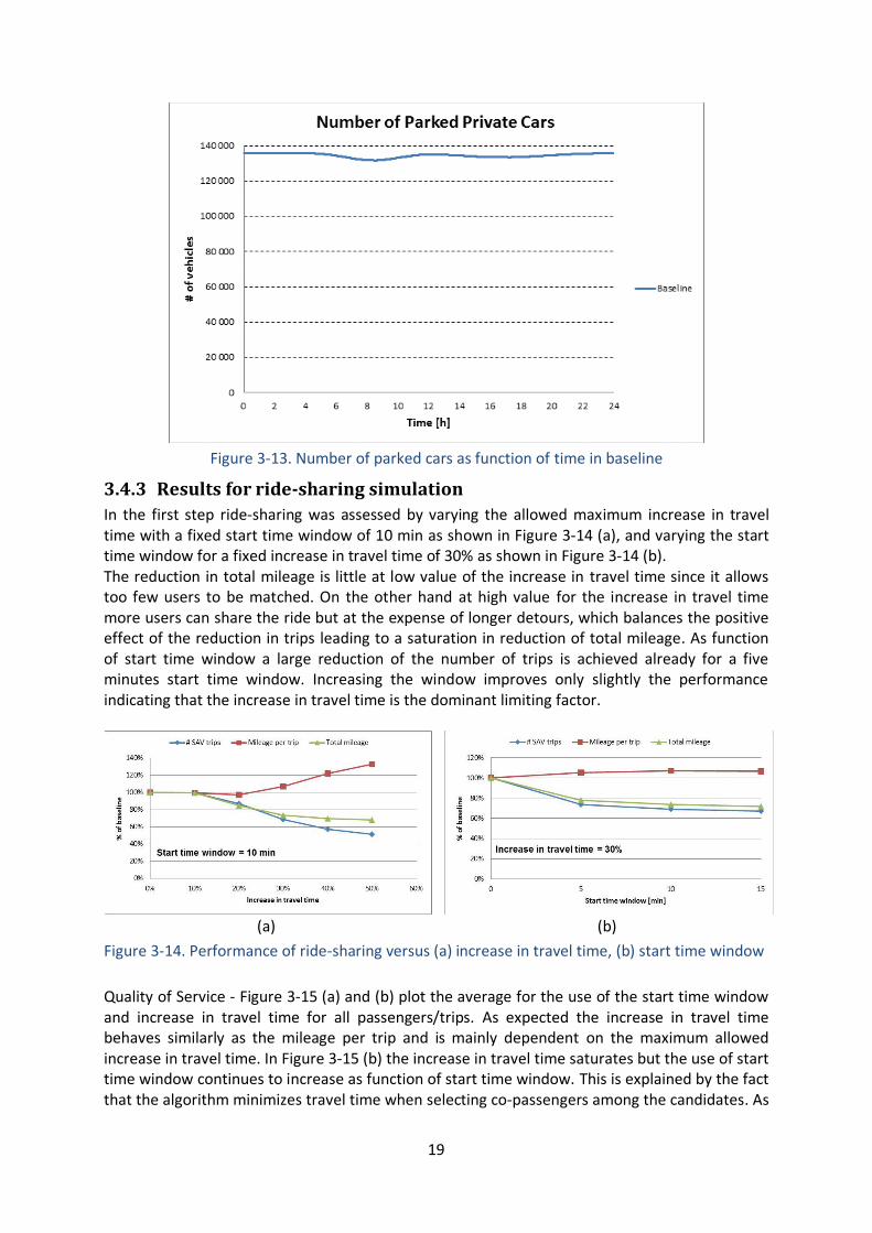
Figure 3-13. Number of parked cars as function of time in baseline

3.4.3 Results for ride-sharing simulation

In the first step ride-sharing was assessed by varying the allowed maximum increase in travel time with a fixed start time window of 10 min as shown in Figure 3-14 (a), and varying the start time window for a fixed increase in travel time of 30% as shown in Figure 3-14 (b). The reduction in total mileage is little at low value of the increase in travel time since it allows too few users to be matched. On the other hand at high value for the increase in travel time more users can share the ride but at the expense of longer detours, which balances the positive effect of the reduction in trips leading to a saturation in reduction of total mileage. As function of start time window a large reduction of the number of trips is achieved already for a five minutes start time window. Increasing the window improves only slightly the performance indicating that the increase in travel time is the dominant limiting factor.

(a) (b)

Figure 3-14. Performance of ride-sharing versus (a) increase in travel time, (b) start time window

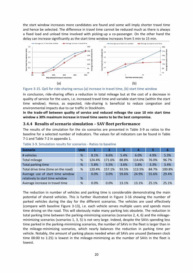
Quality of Service - Figure 3-15 (a) and (b) plot the average for the use of the start time window and increase in travel time for all passengers/trips. As expected the increase in travel time behaves similarly as the mileage per trip and is mainly dependent on the maximum allowed increase in travel time. In Figure 3-15 (b) the increase in travel time saturates but the use of start time window continues to increase as function of start time window. This is explained by the fact that the algorithm minimizes travel time when selecting co-passengers among the candidates. As

20

the start window increases more candidates are found and some will imply shorter travel time and hence be selected. The difference in travel time cannot be reduced much as there is always a fixed load and unload time involved with picking-up a co-passenger. On the other hand the delay can increase significantly as the start time window increases from 5 min to 15 min.

(a) (b)

Figure 3-15. QoS for ride-sharing versus (a) increase in travel time, (b) start time window

In conclusion, ride-sharing offers a reduction in total mileage but at the cost of a decrease in quality of service for the users, i.e. increased travel time and variable start time (within the start time window). Hence, as expected, ride-sharing is beneficial to reduce congestion and environmental impacts due to car traffic in Stockholm. In the trade-off between quality of service and reduced mileage the case 10 min start time window a 30% maximum increase in travel time seems to be the best compromise.

3.4.4 Results of scenario simulation – SAV fleet performance

The results of the simulation for the six scenarios are presented in Table 3-9 as ratios to the baseline for a selected number of indicators. The values for all indicators can be found in Table 7-1 and Table 7-2 in appendix 1.

Table 3-9. Simulation results for scenarios - Ratios to baseline

Scenario Unit 1 2 3 4 5 6

# vehicles % 8.1% 8.6% 5.4% 6.0% 4.9% 5.3%

Total mileage % 124.4% 171.6% 88.8% 114.6% 76.0% 96.7%

Total parking time % 5.8% 5.5% 3.6% 3.8% 3.3% 3.4%

Total drive time (time on the road) % 120.4% 157.1% 93.5% 113.5% 84.7% 100.8%

Average use of start time window relatively to start time window %

0.0% 0.0% 59.6% 24.9% 55.6% 29.4%

Average increase in travel time % 0.0% 0.0% 13.1% 13.1% 25.1% 25.1%

The reduction in number of vehicles and parking time is considerable demonstrating the main potential of shared vehicles. This is further illustrated in Figure 3-16 showing the number of parked vehicles during the day for the different scenarios. The vehicles are used effectively (compare with baseline Figure 3-13), i.e. each vehicle serves multiple users and spends more time driving on the road. This will obviously make many parking lots obsolete. The reduction in total parking time between the parking-minimizing scenarios (scenarios 2, 4, 6) and the mileage-minimizing scenarios (scenarios 1, 3, 5) is not very large. Indeed, despite the SAVs spending less time parked in the parking-minimizing scenarios, the number of SAVs in the fleet is larger than in the mileage-minimizing scenarios, which nearly balances the reduction in parking time per vehicle. Notably, the amount of parking places needed when all SAVs are unused (between clock time 00:00 to 1:25) is lowest in the mileage-minimizing as the number of SAVs in the fleet is lowest.

21

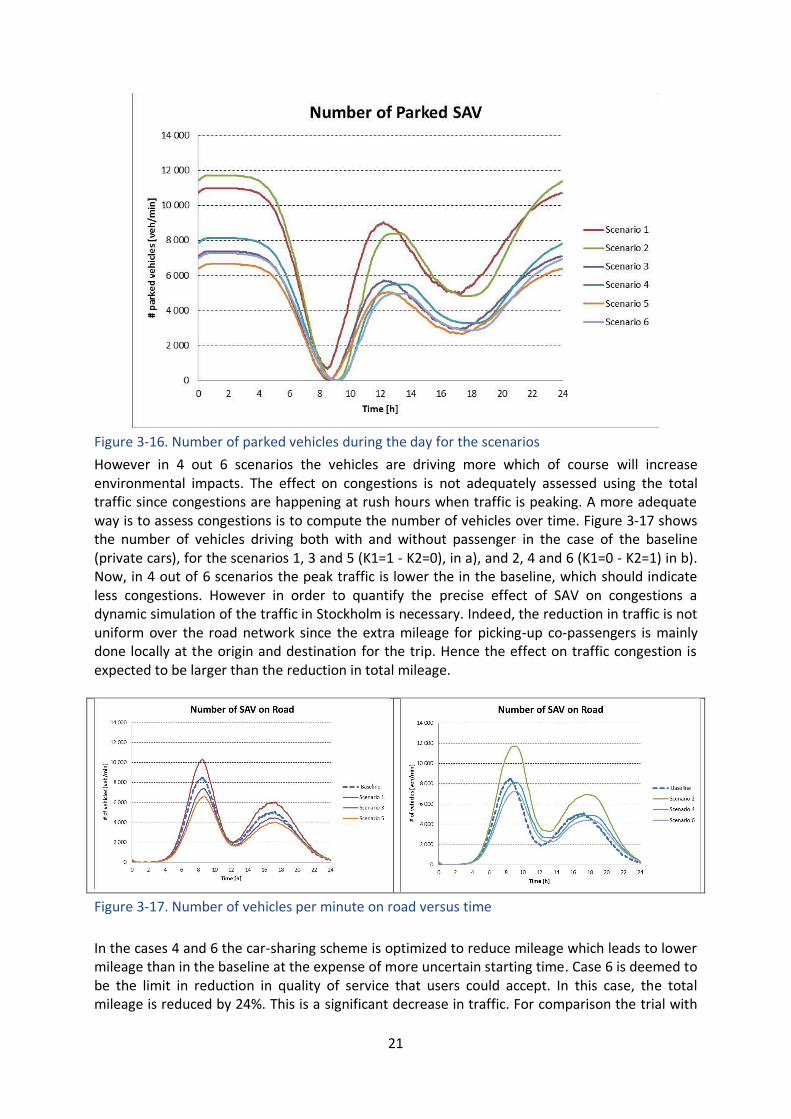
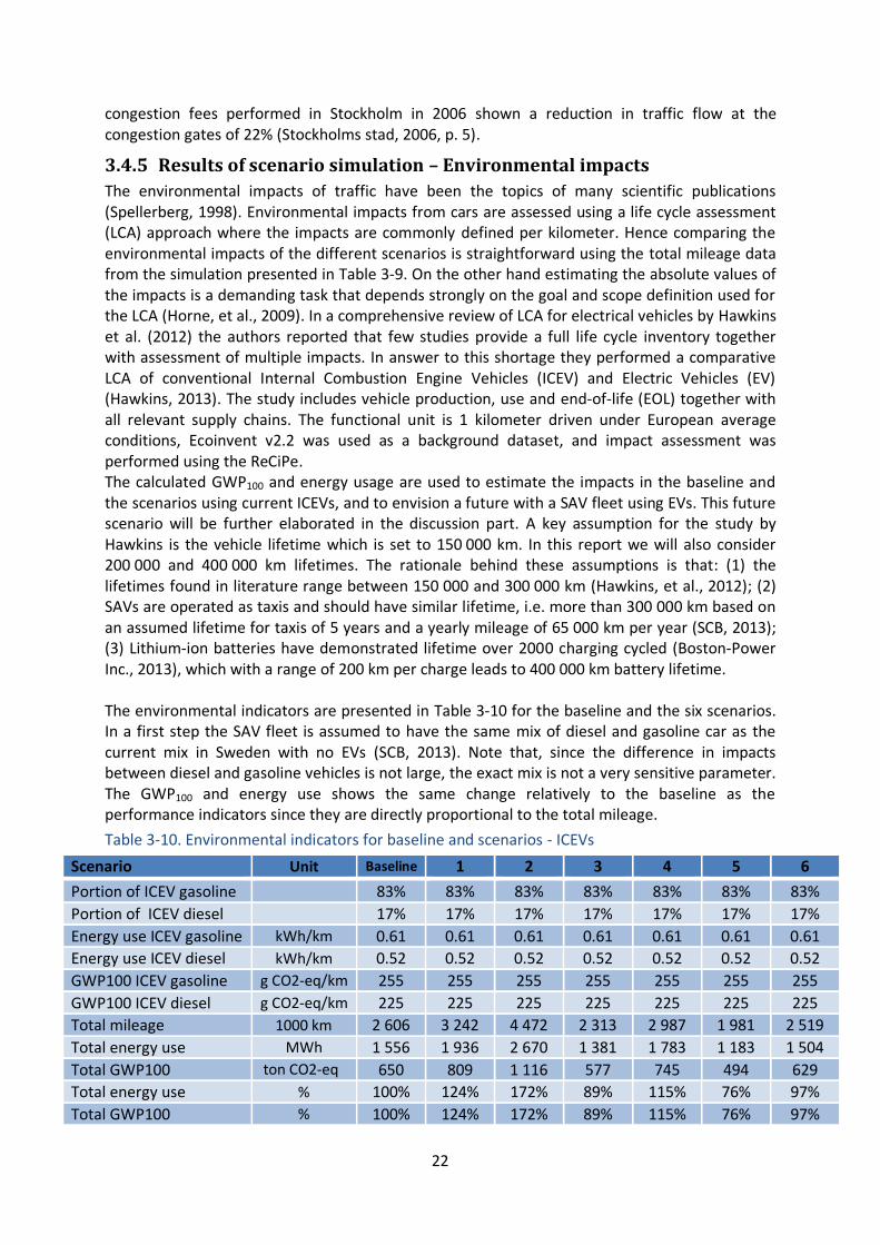
Figure 3-16. Number of parked vehicles during the day for the scenarios

However in 4 out 6 scenarios the vehicles are driving more which of course will increase environmental impacts. The effect on congestions is not adequately assessed using the total traffic since congestions are happening at rush hours when traffic is peaking. A more adequate way is to assess congestions is to compute the number of vehicles over time. Figure 3-17 shows the number of vehicles driving both with and without passenger in the case of the baseline (private cars), for the scenarios 1, 3 and 5 (K1=1 - K2=0), in a), and 2, 4 and 6 (K1=0 - K2=1) in b). Now, in 4 out of 6 scenarios the peak traffic is lower the in the baseline, which should indicate less congestions. However in order to quantify the precise effect of SAV on congestions a dynamic simulation of the traffic in Stockholm is necessary. Indeed, the reduction in traffic is not uniform over the road network since the extra mileage for picking-up co-passengers is mainly done locally at the origin and destination for the trip. Hence the effect on traffic congestion is expected to be larger than the reduction in total mileage.

Figure 3-17. Number of vehicles per minute on road versus time

In the cases 4 and 6 the car-sharing scheme is optimized to reduce mileage which leads to lower mileage than in the baseline at the expense of more uncertain starting time. Case 6 is deemed to be the limit in reduction in quality of service that users could accept. In this case, the total mileage is reduced by 24%. This is a significant decrease in traffic. For comparison the trial with

22

congestion fees performed in Stockholm in 2006 shown a reduction in traffic flow at the congestion gates of 22% (Stockholms stad, 2006, p. 5).

3.4.5 Results of scenario simulation – Environmental impacts

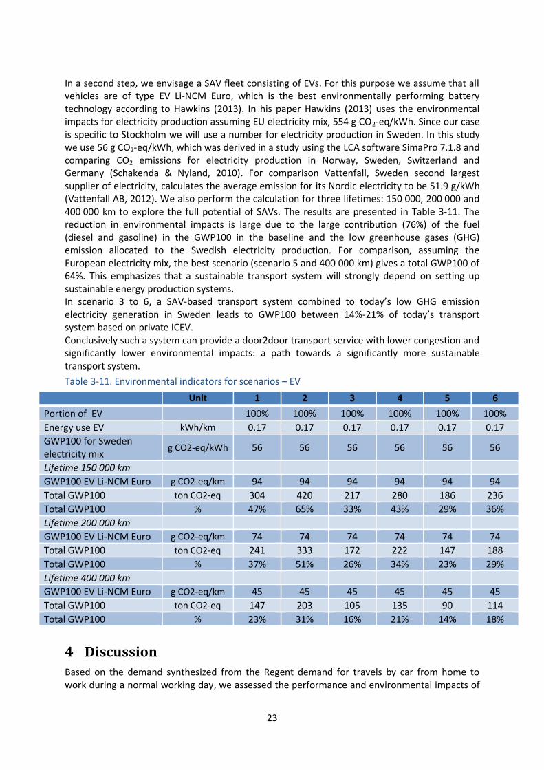
The environmental impacts of traffic have been the topics of many scientific publications (Spellerberg, 1998). Environmental impacts from cars are assessed using a life cycle assessment (LCA) approach where the impacts are commonly defined per kilometer. Hence comparing the environmental impacts of the different scenarios is straightforward using the total mileage data from the simulation presented in Table 3-9. On the other hand estimating the absolute values of the impacts is a demanding task that depends strongly on the goal and scope definition used for the LCA (Horne, et al., 2009). In a comprehensive review of LCA for electrical vehicles by Hawkins et al. (2012) the authors reported that few studies provide a full life cycle inventory together with assessment of multiple impacts. In answer to this shortage they performed a comparative LCA of conventional Internal Combustion Engine Vehicles (ICEV) and Electric Vehicles (EV) (Hawkins, 2013). The study includes vehicle production, use and end-of-life (EOL) together with all relevant supply chains. The functional unit is 1 kilometer driven under European average conditions, Ecoinvent v2.2 was used as a background dataset, and impact assessment was performed using the ReCiPe. The calculated GWP100 and energy usage are used to estimate the impacts in the baseline and the scenarios using current ICEVs, and to envision a future with a SAV fleet using EVs. This future scenario will be further elaborated in the discussion part. A key assumption for the study by Hawkins is the vehicle lifetime which is set to 150 000 km. In this report we will also consider 200 000 and 400 000 km lifetimes. The rationale behind these assumptions is that: (1) the lifetimes found in literature range between 150 000 and 300 000 km (Hawkins, et al., 2012); (2) SAVs are operated as taxis and should have similar lifetime, i.e. more than 300 000 km based on an assumed lifetime for taxis of 5 years and a yearly mileage of 65 000 km per year (SCB, 2013); (3) Lithium-ion batteries have demonstrated lifetime over 2000 charging cycled (Boston-Power Inc., 2013), which with a range of 200 km per charge leads to 400 000 km battery lifetime. The environmental indicators are presented in Table 3-10 for the baseline and the six scenarios. In a first step the SAV fleet is assumed to have the same mix of diesel and gasoline car as the current mix in Sweden with no EVs (SCB, 2013). Note that, since the difference in impacts between diesel and gasoline vehicles is not large, the exact mix is not a very sensitive parameter. The GWP100 and energy use shows the same change relatively to the baseline as the performance indicators since they are directly proportional to the total mileage.

Table 3-10. Environmental indicators for baseline and scenarios - ICEVs

Scenario Unit Baseline 1 2 3 4 5 6

Portion of ICEV gasoline 83% 83% 83% 83% 83% 83% 83%

Portion of ICEV diesel 17% 17% 17% 17% 17% 17% 17%

Energy use ICEV gasoline kWh/km 0.61 0.61 0.61 0.61 0.61 0.61 0.61

Energy use ICEV diesel kWh/km 0.52 0.52 0.52 0.52 0.52 0.52 0.52

GWP100 ICEV gasoline g CO2-eq/km 255 255 255 255 255 255 255

GWP100 ICEV diesel g CO2-eq/km 225 225 225 225 225 225 225

Total mileage 1000 km 2 606 3 242 4 472 2 313 2 987 1 981 2 519

Total energy use MWh 1 556 1 936 2 670 1 381 1 783 1 183 1 504

Total GWP100 ton CO2-eq 650 809 1 116 577 745 494 629

Total energy use % 100% 124% 172% 89% 115% 76% 97%

Total GWP100 % 100% 124% 172% 89% 115% 76% 97%

23

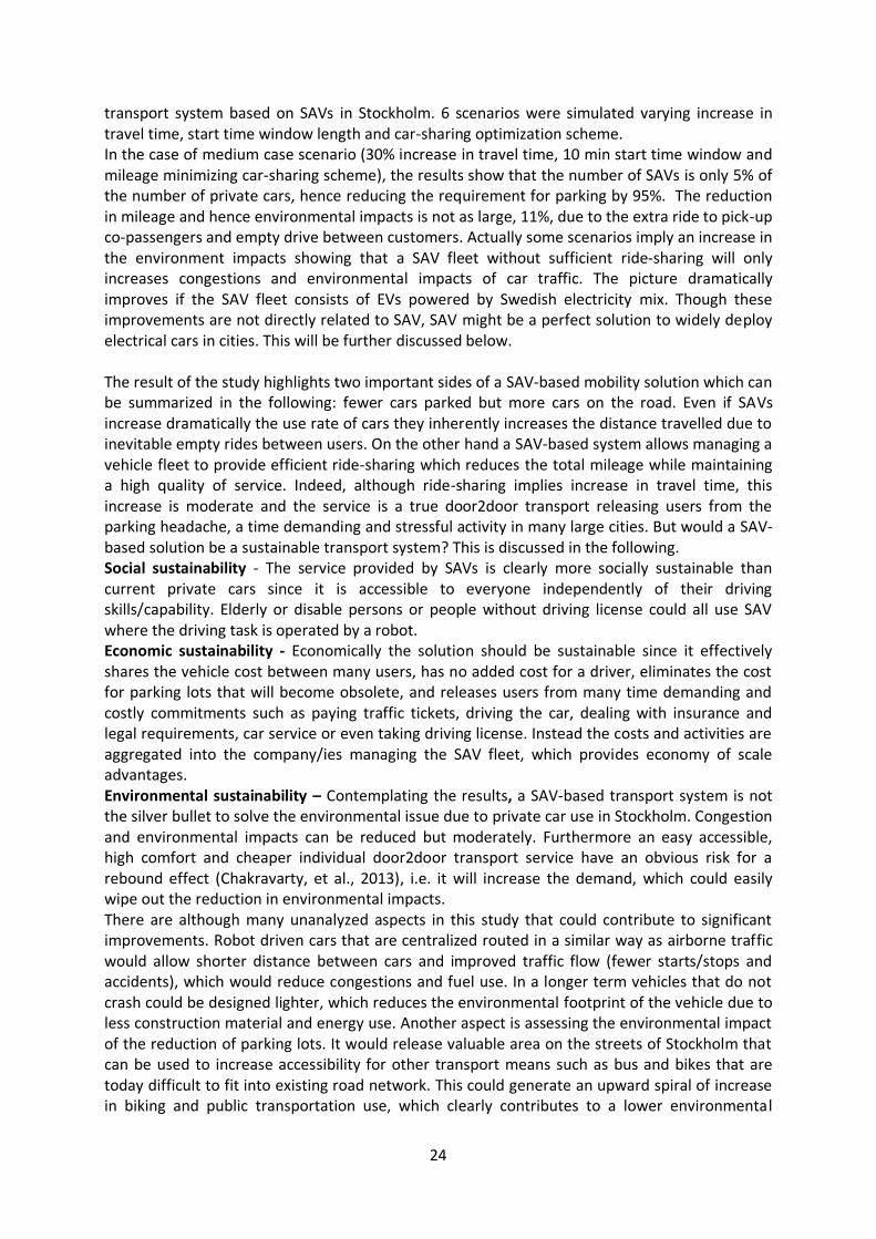
In a second step, we envisage a SAV fleet consisting of EVs. For this purpose we assume that all vehicles are of type EV Li-NCM Euro, which is the best environmentally performing battery technology according to Hawkins (2013). In his paper Hawkins (2013) uses the environmental impacts for electricity production assuming EU electricity mix, 554 g CO2-eq/kWh. Since our case is specific to Stockholm we will use a number for electricity production in Sweden. In this study we use 56 g CO2-eq/kWh, which was derived in a study using the LCA software SimaPro 7.1.8 and comparing CO2 emissions for electricity production in Norway, Sweden, Switzerland and Germany (Schakenda & Nyland, 2010). For comparison Vattenfall, Sweden second largest supplier of electricity, calculates the average emission for its Nordic electricity to be 51.9 g/kWh (Vattenfall AB, 2012). We also perform the calculation for three lifetimes: 150 000, 200 000 and 400 000 km to explore the full potential of SAVs. The results are presented in Table 3-11. The reduction in environmental impacts is large due to the large contribution (76%) of the fuel (diesel and gasoline) in the GWP100 in the baseline and the low greenhouse gases (GHG) emission allocated to the Swedish electricity production. For comparison, assuming the European electricity mix, the best scenario (scenario 5 and 400 000 km) gives a total GWP100 of 64%. This emphasizes that a sustainable transport system will strongly depend on setting up sustainable energy production systems. In scenario 3 to 6, a SAV-based transport system combined to today’s low GHG emission electricity generation in Sweden leads to GWP100 between 14%-21% of today’s transport system based on private ICEV. Conclusively such a system can provide a door2door transport service with lower congestion and significantly lower environmental impacts: a path towards a significantly more sustainable transport system.

Table 3-11. Environmental indicators for scenarios – EV

Unit 1 2 3 4 5 6

Portion of EV 100% 100% 100% 100% 100% 100%

Energy use EV kWh/km 0.17 0.17 0.17 0.17 0.17 0.17

GWP100 for Sweden electricity mix

g CO2-eq/kWh 56 56 56 56 56 56

Lifetime 150 000 km

GWP100 EV Li-NCM Euro g CO2-eq/km 94 94 94 94 94 94

Total GWP100 ton CO2-eq 304 420 217 280 186 236

Total GWP100 % 47% 65% 33% 43% 29% 36%

Lifetime 200 000 km

GWP100 EV Li-NCM Euro g CO2-eq/km 74 74 74 74 74 74

Total GWP100 ton CO2-eq 241 333 172 222 147 188

Total GWP100 % 37% 51% 26% 34% 23% 29%

Lifetime 400 000 km

GWP100 EV Li-NCM Euro g CO2-eq/km 45 45 45 45 45 45

Total GWP100 ton CO2-eq 147 203 105 135 90 114

Total GWP100 % 23% 31% 16% 21% 14% 18%

4 Discussion

Based on the demand synthesized from the Regent demand for travels by car from home to work during a normal working day, we assessed the performance and environmental impacts of

24

transport system based on SAVs in Stockholm. 6 scenarios were simulated varying increase in travel time, start time window length and car-sharing optimization scheme. In the case of medium case scenario (30% increase in travel time, 10 min start time window and mileage minimizing car-sharing scheme), the results show that the number of SAVs is only 5% of the number of private cars, hence reducing the requirement for parking by 95%. The reduction in mileage and hence environmental impacts is not as large, 11%, due to the extra ride to pick-up co-passengers and empty drive between customers. Actually some scenarios imply an increase in the environment impacts showing that a SAV fleet without sufficient ride-sharing will only increases congestions and environmental impacts of car traffic. The picture dramatically improves if the SAV fleet consists of EVs powered by Swedish electricity mix. Though these improvements are not directly related to SAV, SAV might be a perfect solution to widely deploy electrical cars in cities. This will be further discussed below. The result of the study highlights two important sides of a SAV-based mobility solution which can be summarized in the following: fewer cars parked but more cars on the road. Even if SAVs increase dramatically the use rate of cars they inherently increases the distance travelled due to inevitable empty rides between users. On the other hand a SAV-based system allows managing a vehicle fleet to provide efficient ride-sharing which reduces the total mileage while maintaining a high quality of service. Indeed, although ride-sharing implies increase in travel time, this increase is moderate and the service is a true door2door transport releasing users from the parking headache, a time demanding and stressful activity in many large cities. But would a SAV-based solution be a sustainable transport system? This is discussed in the following. Social sustainability - The service provided by SAVs is clearly more socially sustainable than current private cars since it is accessible to everyone independently of their driving skills/capability. Elderly or disable persons or people without driving license could all use SAV where the driving task is operated by a robot. Economic sustainability - Economically the solution should be sustainable since it effectively shares the vehicle cost between many users, has no added cost for a driver, eliminates the cost for parking lots that will become obsolete, and releases users from many time demanding and costly commitments such as paying traffic tickets, driving the car, dealing with insurance and legal requirements, car service or even taking driving license. Instead the costs and activities are aggregated into the company/ies managing the SAV fleet, which provides economy of scale advantages. Environmental sustainability – Contemplating the results, a SAV-based transport system is not the silver bullet to solve the environmental issue due to private car use in Stockholm. Congestion and environmental impacts can be reduced but moderately. Furthermore an easy accessible, high comfort and cheaper individual door2door transport service have an obvious risk for a rebound effect (Chakravarty, et al., 2013), i.e. it will increase the demand, which could easily wipe out the reduction in environmental impacts. There are although many unanalyzed aspects in this study that could contribute to significant improvements. Robot driven cars that are centralized routed in a similar way as airborne traffic would allow shorter distance between cars and improved traffic flow (fewer starts/stops and accidents), which would reduce congestions and fuel use. In a longer term vehicles that do not crash could be designed lighter, which reduces the environmental footprint of the vehicle due to less construction material and energy use. Another aspect is assessing the environmental impact of the reduction of parking lots. It would release valuable area on the streets of Stockholm that can be used to increase accessibility for other transport means such as bus and bikes that are today difficult to fit into existing road network. This could generate an upward spiral of increase in biking and public transportation use, which clearly contributes to a lower environmental

25

impacts and reaching the goals set in Stockholm’s vision 2030 (Stockholmsstad, 2014). A last aspect is the use of SAV fleet consisting of EVs. This is discussed in the section below. Electrical vehicles + SAV - In the result section we analyzed the case of a SAV fleet consisting of EVs powered by Swedish electricity mix. As a consequence of the low emissions for the electricity production in Sweden the GWP100 is less than 20% of the GWP100 in the baseline where most of the vehicles are powered by fossil fuel. Electrical vehicles are advertised as zero local emission, superior engine efficiency, compatible with many renewable energies production, great performance, and low noise. In spite of these advantages and the great technology developments this last decade, there are still obstacles to the wider introduction of electric vehicles. These include the long charging times, shorter driving range and the skepticism among potential end-users (Fabian Kley, 2011; Theo Lieven, 2011). A SAV-based system circumvents these hurdles. First the SAV ownership structure addresses the concern about high purchase cost of electrical vehicles since this cost is carried by the service company which can share this cost between many users. Second the charging time and driving range issues can be included in the management of the SAV fleet. Indeed the mileage of the SAV per day is in the range of 300-400 km (see Appendix 1), which would require 1 to 3 charging sessions depending on the EV driving range. Today’s charging capacity of EVs expressed as kilometers per charging hour is between 320 to 480 km/h using superchargers (Nissan, 2014; Renault, 2014; Tesla Motors, 2014) implying that the total charging time per day for the SAVs should be around 1 hour. A faster alternative to charging is battery swap which takes 90 seconds on a Tesla model S (Tesla Motors, 2014). With an infrastructure of superchargers or battery swap stations and appropriate management of the SAV fleet operation, the charging issue can be readily resolved by adding requirement for time for charging or battery switch. Moreover the charging or battery swap infrastructure can be located at a limited number of sites in Stockholm, and shared by many SAVS. This lowers the cost of the infrastructure, simplifies the service of the equipment, and eliminate the need of deploying a costly and certainly not problem free charging infrastructure “on streets” in Stockholm. Conclusively a SAV-based system and EV technology seems to be a “perfect” match that could definitely contribute to a sustainable transport system for Stockholm. Limitations of the study This study provides an initial assessment of the implementation of a transport service using a fleet of shared autonomous vehicles in Stockholm metropolitan area and it has clearly a number of limitations. (1) Only internal traffic is accounted which, although represents about 60% of whole car traffic

in Stockholm, leaves a large trunk of traffic unaddressed. (2) The demand is synthesized based on a survey and involves several calculation steps and

assumptions. The total amount of traffic seems to be adequate but the detailed patterns in traffic flow have not been verified and compared to real traffic data.

(3) Obviously the simulation is based on a simple model since it does not include dynamic traffic simulation and uses “simple” ride-sharing and car-sharing algorithms. To achieve a more accurate picture of the effects of the implementation of a SAV system in Stockholm a more advanced modeling is necessary.

Significance of the study Car traffic is impacting the environmental performance of Stockholm. The CO2-eq emission from road transport locally in Stockholm region is about 1 ton CO2-eq per inhabitant, which represents 40% of total emissions (Stockholmsstad, 2014). The number of private cars included in this study is 135 934 which is about 50% of the cars included in the Regent demand describing

26

the traffic in Stockholm County. For comparison the total number of private cars registered in Stockholm County was 941 954 in 2013 (Trafik Analys, 2014) and the population was 2 163 042 (Statistika centralbyrån, 2014). According to (Stockholmsstad, 2013), 50% of trips by car in Stockholm County are less than 5 km. The technology of autonomous vehicles will doubtless be available in all cars within the next two decades with enhanced safety being the main driving force. This study provides another vision showing that the technology can enable a transport system that could advantageously replace the current system based on private car ownership. Such a SAV-based system will not only revolutionize transportation systems but also deeply change the significance of car in our society, e.g. car ownership, car industry and the way cities are designed. Comparing to other published works The results of the study can be put in relation to other works though there are few published studies assessing SAV-based transport system. The study from Fagnant & Kockelman (2014) uses a theoretical grid network with a synthesized demand based on national travel statistics in the US to simulate the travel and environmental implications of SAVs. Importantly the study does not include ride-sharing. Fagnant & Kockelman show that the number of car is 10% the number of private cars and the total mileage increases by 11%, which is in par with our results when assuming no ride-sharing. The assessment in change in environmental impacts follows a similar LCA approach as done in the study of Stockholm. Despite the increase in total mileage Fagnant & Kockelman show a reduction in GHG emissions and energy use of 5.6% and 12% respectively. Three reasons are provided to explain the reduction: the use of single type of car (medium size) for the SAV fleet, which replaces less fuel efficient pickup trucks, SUVs and minivans and represents 47% of all vehicles; the reduction in parking infrastructure; the reduction in vehicle starts and cold starts. Unsatisfactorily the change in environmental impacts is not reported individually for each of these reasons making difficult to compare with our results. Another work by Kornhauser et al. (2013) assesses the use of a SAV system operating through New Jersey’s roadways, where passengers are load and unloaded at stations available within at most a short walk distance (< 5 min). The synthesized demand corresponds to 32+ millions of trips made by New Jersey’s 9 million inhabitants, where 90% is car traffic. The study includes two ride-sharing schemes: (1) ride-sharing with SAV waiting a fixed amount of time for additional passengers destined to any destinations that incurred less than a 20% detour for any passenger; (2) ride-sharing where the SAV sweeps up a local area to pick-up co-passenger with close-by destination and about the same start time. The SAV-based system simulated by Kornhauser differs significantly from the system studied in this report as it assumes that 14.8% of the trips are served by a combining SAV and railways and the ride-sharing-schemes simulated do not provide a pure door-2-door service. Though, they are close enough to allow comparing results. The average vehicle occupancy (AVO) is defined as the ratio between the passenger mileage and the vehicle mileage. For ride-sharing scheme 1 with one stop and 5 min waiting time the AVO reaches 2. For scheme 2 with squared pick-up and destination areas of 5 km the AVO is 2.16. These numbers are once more in par the average number of passengers per SAV obtained in Stockholm. Although the AVO is significantly larger indicating a more efficient ride-sharing scheme or a more ride-sharing friendly trip demand. The fleet size needed to serve the New Jersey demand is 45% of the current private car fleet indicating that the cars are not serving as many trips during the day as in the case of Stockholm. A third paper provides analytical guidelines for the design of SAV mobility systems without ride-sharing, which are applied to the specific case of Singapore (Spieser, et al., 2014) to dimension a SAV fleet to serve all ground transport (bus, subway, cars). The trip demand is evaluated from a comprehensive survey gathering information of high-level transportation patterns in Singapore. The trip demand

27

includes nearly 5.6 million trips. The road network is a graph-based representation of Singapore’s road network, and the traffic characteristics (speed and congestions) is estimated using GPS coordinates from about 15 000 taxis (60% of all taxis). The results show that the fleet size needed to keep waiting times below 15 min at all time is 300 000 vehicles. This implies that each vehicle is in average serving 20 trips/users per day. In our study in Stockholm, the equivalent number is between 23 and 41 depending on the scenario. Note that the number of trips/users served is expected to be larger in the study of Stockholm since it includes ride-sharing which is not part of the analysis of Singapore. Future work Autonomous vehicles open a wide field for future work since it is foreseen to have many implications in our car-centered society. It could touch areas related to:

Economy: studying the business models for the companies operating SAV fleets, or the implications in the car industry when cars will be designed for rational companies instead of emotional individuals;

Social aspects: safety, legal responsibility in case of accident, possible rebound effects, personal identity related to car ownership, or the psychological aspects like thresholds and acceptance for robot driven cars.

Urbanism: what to do with the freed space when most of the parking places are obsolete? Do we need to design specific loading and unloading zones? Would the requirements for road infrastructure, e.g. traffic signals, road lights, road construction, change?

Technology: how car would look like when there is no need for steering wheel and driver place?

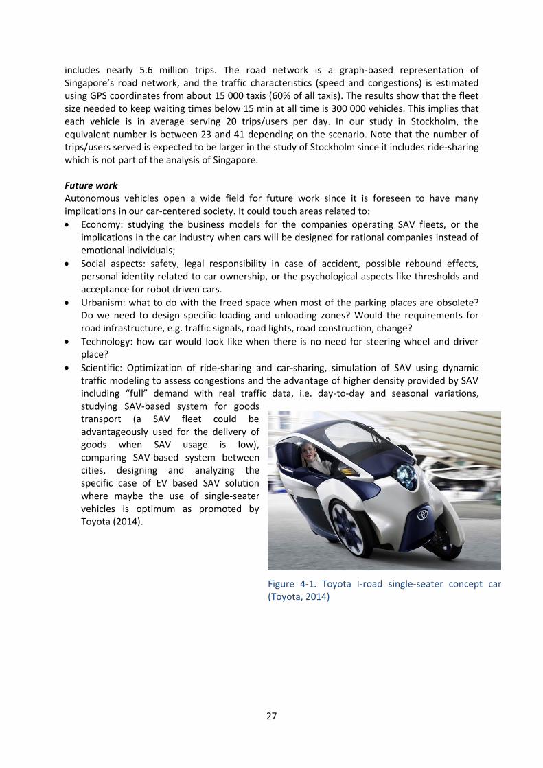
Scientific: Optimization of ride-sharing and car-sharing, simulation of SAV using dynamic traffic modeling to assess congestions and the advantage of higher density provided by SAV including “full” demand with real traffic data, i.e. day-to-day and seasonal variations, studying SAV-based system for goods transport (a SAV fleet could be advantageously used for the delivery of goods when SAV usage is low), comparing SAV-based system between cities, designing and analyzing the specific case of EV based SAV solution where maybe the use of single-seater vehicles is optimum as promoted by Toyota (2014).

Figure 4-1. Toyota I-road single-seater concept car (Toyota, 2014)

28

5 Conclusion

In this report we studied potential benefits of a fleet of shared autonomous vehicles (SAV) providing a taxi service replacing private car commuter trips in a metropolitan area. We developed a framework for dynamic allocation of SAV to passenger trips, empty-vehicle routing and multi-criteria evaluation with regard to passenger waiting time, trip times and fleet size. Using the Stockholm metropolitan area as a case, we evaluate a number of ride-sharing scenarios, varying the accepted start time window and acceptable travel time increase with ride-sharing. In a following step the environmental impacts of the different scenarios are assessed and compared using a life cycle assessment methodology. The assessment includes both a fleet consisting of currently in use gasoline and diesel cars as well as electrical cars. Our results show that: 1 - An SAV-based personal transport system has the potential to provide an on-demand door2door transport service with a high level of service using less than 10% of today’s private cars and parking places, which is consistent with results reported in the literature. 2 - In a scenario where users are not inclined to accept any reduced level of service, i.e. ride-sharing (no co-passenger) and no delay, empty vehicle drive of an SAV-based personal transport system will increase road traffic and environmental impact. 3 – In order to provide an environmental benefit and lower congestion, the SAV-based personal transport system requires users to accept a max 30% increase in travel time (13% on average) and 10 min start time window. In this case mileage is reduced to 89% of the baseline case, using only 5% of the today’s vehicles and parking places. Contemplating the results, a SAV-based transport system is not the silver bullet to solve the environmental issue due to private car use in Stockholm. Congestion and environmental impacts can be reduced but moderately. Furthermore an easy accessible, high comfort and cheaper individual door2door transport service have an obvious risk for a rebound effect, i.e. it could increase the demand, which could easily wipe out the reduction in environmental impacts. However it is clearly an appealing solution since it makes obsolete most of parking places releasing considerable amount of valuable space in cities. Space that could be used for cycling or public transportation infrastructure, which are difficult to squeeze in today’s city road network. Moreover SAV-based personal transport system is expected to lead to a capacity and safety increase in the road network thanks to the possibility of a centralized traffic planning allowing optimization of traffic flow, reduced distance between vehicles, fewer accidents as human error is suppressed. However, in order to verify this statement dynamic traffic simulation would be necessary. Envisioning a SAV fleet using electrical cars a SAV-based system and electrical vehicle technology seems to be a “perfect” match, where the drawback generally associated to electrical vehicles are circumvented. In combination with renewable electricity production it could definitely contribute to a sustainable transport system in Stockholm.

29

6 References

Boston-Power Inc., 2013. Boston-power.com. [Online] Available at: http://www.boston-power.com/technology/long-life [Accessed 17 June 2014].

Burghout, W., 2004. Hybrid microscopic-mesoscopic traffic simulation. In: Stockholm: KTH.

Chakravarty, D., Dasgupta, S. & Roy, J., 2013. Rebound effect: how much to worry?. Current Opinion in Environmental Sustainability, 5(2), pp. 216-228.

Chapman, L., 2007. Transport and climate change: a review. Journal of Transport Geography, 15(5), pp. 354-367.

Fabian Kley, C., 2011. New businessmodelsforelectriccars—A holisticapproach. Energy Policy, 39(6), pp. 3392-3403.

Fagnant, D. J. & Kockelman, K. M., 2014. The travel and environmental implications of shared autonomous vehicles, using agent-based model scenarios. Transportation Research Part C, Volume 40, pp. 1-13.

Forward, S., 2008. Driving Violations, Uppsala: Uppsala University.

Google, 2014. google.se. [Online] Available at: https://www.google.se/maps/preview [Accessed 3 June 2014].

Gröna Bilister, 2014. gronabilister.se. [Online] Available at: http://www.gronabilister.se/lankar/att-samaka [Accessed 28 May 2014].

Hawkins, T., Gausen, O. & Strømman, A., 2012. Environmental impacts of hybrid and electric vehicles—a review. The International Journal of Life Cycle Assessment, 17(8), pp. 997-1014.

Hawkins, T. R. B. S. G. M.-B. a. A. H. S., 2013. Corrigendum to: Hawkins, T. R., B. Singh, G. Majeau-Bettez, and A. H. Strømman. 2012. Comparative environmental life cycle assessment of conventional and electric vehicles. Journal of Industrial Ecology, 17(1), p. 158–160.

Horne, R., Grant, T. & Verghese, K., 2009. Life cycle assessment in practice. In: Life Cycle Assessment: Principles, Practice and Prospects. Colinwood: CSIRO, pp. 23-31.

INRO, 2014. inrosoftware.com. [Online] Available at: http://www.inrosoftware.com/en/products/emme/ [Accessed 4 August 2014].

Jonsson, D., Berglund, S., Almström, P. & Algers, S., 2011. The usefulness of transport models in Swedish planning practice. Transport Reviews, 31(2), pp. 251-265.

Kevin Spieser, K. T. R. Z. E. F. D. M. a. M. P., 2014. Toward a Systematic Approach to the Design and Evaluation of Automated Mobility-on-Demand Systems - A Case Study in Singapore, s.l.: MIT / Springer.

Knight, W., 2013. MIT Technology Review. [Online] Available at: http://www.technologyreview.com/featuredstory/520431/driverless-cars-are-further-away-than-you-think/ [Accessed 20 May 2014].

30

Kornhauser, A. L., 2013. Smart driving cars. [Online] Available at: http://smartdrivingcar.com/ataxis-for-nj-08.11.13.html [Accessed 24 November 2013].

Krisher, T., 2013. USA today. [Online] Available at: http://www.usatoday.com/story/money/cars/2013/08/30/gm-general-motors-self-driving-autonomous-car/2725091/ [Accessed 3 October 2013].

Lawrence D. Burns, W. C. J., 2012. Transforming Personal Mobility, Scarborough BA: The Earth Institute. Columbia University.

Marks, P., 2012. Hands off the wheel. New Scientist, 31 Mars, p. 19.

Movea Trafikkonsult, 2014. Movea. [Online] Available at: http://www.movea.se/Index-filer/Page4149.htm [Accessed 21 May 2014].

Nissan, 2013. NissanNews. [Online] Available at: http://nissannews.com/en-US/nissan/usa/releases/nissan-announces-unprecedented-autonomous-drive-benchmarks [Accessed 3 October 2013].

Nissan, 2014. nissan.se. [Online] Available at: http://www.nissan.se/SE/sv/vehicle/electric-vehicles/leaf/charging-and-battery/range.html [Accessed 27 June 2014].

PTV Group, 2014. http://vision-traffic.ptvgroup.com/. [Online] Available at: http://vision-traffic.ptvgroup.com/en-us/products/ptv-visum/ [Accessed 4 August 2014].

Quick, D., 2009. gizmag.com. [Online] Available at: http://www.gizmag.com/environmental-assessment-passenger-transport/11953/ [Accessed 29 August 2014].

Regeringskansliet, 2008. En sammanhållen klimat- och energipolitik, Stockholm: Regeringskansliet.

Renault, 2014. renault.se. [Online] Available at: http://www.renault.se/media/Broschyrer/atte88e99eb4569453b8df9b8e087f17858/ZOE_B10_final_140415.pdf [Accessed 27 June 2014].

Rosenbush, S., 2013. Under Pressure, Google May Slow Rollout of Driverless Car Technology. Wall Street Journal, 18 July.

SCB, 2013. Årsbok 2013, Stockholm: Statiska Centralbyrån.

Schakenda, V. & Nyland, C. A., 2010. ostfoldforskning.no. [Online] Available at: http://ostfoldforskning.no/uploads/dokumenter/publikasjoner/627.pdf [Accessed 1 June 2014].

Shankland, S., 2013. CNET. [Online] Available at: http://www.cnet.com/news/self-driving-cars-will-bristle-with-sensors/ [Accessed 20 May 2014].

31

Spellerberg, I., 1998. Ecological effects of roads and traffic: a literature review. Global Ecology and Biogeography, 7(5), pp. 317-333.

Spieser, K. et al., 2014. DSpace@MIT. [Online] Available at: http://dspace.mit.edu/handle/1721.1/82904 [Accessed 20 April 2014].

Statens energimyndighet, 2013. Transportsektorns energianvändning 2012, Eskilstuna: Statens energimyndighet.

Statistika centralbyrån, 2014. scb.se. [Online] Available at: http://www.scb.se/sv_/Hitta-statistik/Statistik-efter-amne/Befolkning/Befolkningens-sammansattning/Befolkningsstatistik/25788/25795/Helarsstatistik---Kommun-lan-och-riket/370301/ [Accessed 1 June 2014].

Stockholms stad, 2006. Fakta och resultat från Stockholmsförsöket, Stockholm: Stockholms stad.

Stockholmsförsöket, 2006. stockholmsforsoket.se. [Online] Available at: http://www.stockholmsforsoket.se/templates/page.aspx?id=10930 [Accessed 21 May 2014].

Stockholmsstad, 2013. stockholm.se. [Online] Available at: http://www.stockholm.se/TrafikStadsplanering/Trafik-och-resor-/Trafik-och-miljo/ [Accessed 2 June 2014].

Stockholmsstad, 2013. stockholm.se. [Online] Available at: http://www.stockholm.se/ByggBo/Leva-Miljovanligt/Klimatsmart-resande/ [Accessed 1 June 2014].

Stockholmsstad, 2014. miljobarometern.stockholm.se. [Online] Available at: http://miljobarometern.stockholm.se/key.asp?mo=1&dm=1&nt=2 [Accessed 2 June 2014].

Stockholmsstad, 2014. stockholm.se. [Online] Available at: http://www.stockholm.se/OmStockholm/Vision-2030/ [Accessed 25 June 2014].

Sweeting, W. J. & Winfield, P. H., 2012. Future transportation: Lifetime considerations and framework for sustainability assessment. Energy Policy, Volume 51, pp. 927-938.

Taylor, N. B., 2003. The CONTRAM Dynamic Traffic Assignment Model. Networks and Spatial Economics, 3(3), pp. 297-322.

Tesla Motors, 2014. teslamotors.com. [Online] Available at: http://www.teslamotors.com/sv_SE/charging#/onthego [Accessed 27 June 2014].

Tesla Motors, 2014. teslamotors.com. [Online] Available at: http://www.teslamotors.com/batteryswap [Accessed 27 June 2014].

The Economist, 2012. Look, no hands. The Economist, 1 September.

The Economist, 2014. In the self-driving seat. The Economis, 31 May.

Theo Lieven, S. M. S. H. J. F. W., 2011. Who will buy electric cars? An empirical study in Germany. Transportation Research Part D: Transport and Environment, 16(3), pp. 236-243.

32

Thrun, S., 2010. Toward Robotic Cars. Communications of the ACM, 53(4), p. April.

TomTom, 2013. tomtom.com. [Online] Available at: http://www.tomtom.com/lib/doc/trafficindex/2013-1101%20TomTomTrafficIndex2013Q2EUR-km.pdf [Accessed 19 May 2014].

Toyota, 2014. toyota-global.com. [Online] Available at: http://www.toyota-global.com/innovation/personal_mobility/i-road/ [Accessed 30 June 2014].

Trafik Analys, 2014. trafa.se. [Online] Available at: http://trafa.se/PageDocuments/Fordon_i_laen_och_kommuner_2013.pdf [Accessed 1 June 2014].

Trafikanalys, 2014. trafa.se. [Online] Available at: http://www.trafa.se/sv/malportal/Indikatorer/Genomsnittlig-korstracka-per-ar-for-personbilar-agda-av-fysiska-personer/?Region=0&Text=about [Accessed 20 May 2014].

Vattenfall AB, 2012. corporate.vattenfall.com. [Online] Available at: http://corporate.vattenfall.com/Global/corporate/sustainability/doc/life_cycle_assessment.pdf [Accessed 8 Augusti 2014].

Volvo Car Group, 2013. volvocars.com. [Online] Available at: http://www.volvocars.com/se/top/about/news-events/pages/default.aspx?itemid=470 [Accessed 20 May 2014].

World Bank, 2014. The World Bank. [Online] Available at: http://data.worldbank.org/indicator/IS.VEH.PCAR.P3/countries?display=graph [Accessed 12 May 2014].

World Health Organisation, 2014. who.int. [Online] Available at: http://www.who.int/gho/urban_health/situation_trends/urban_population_growth_text/en/ [Accessed 19 May 2014].

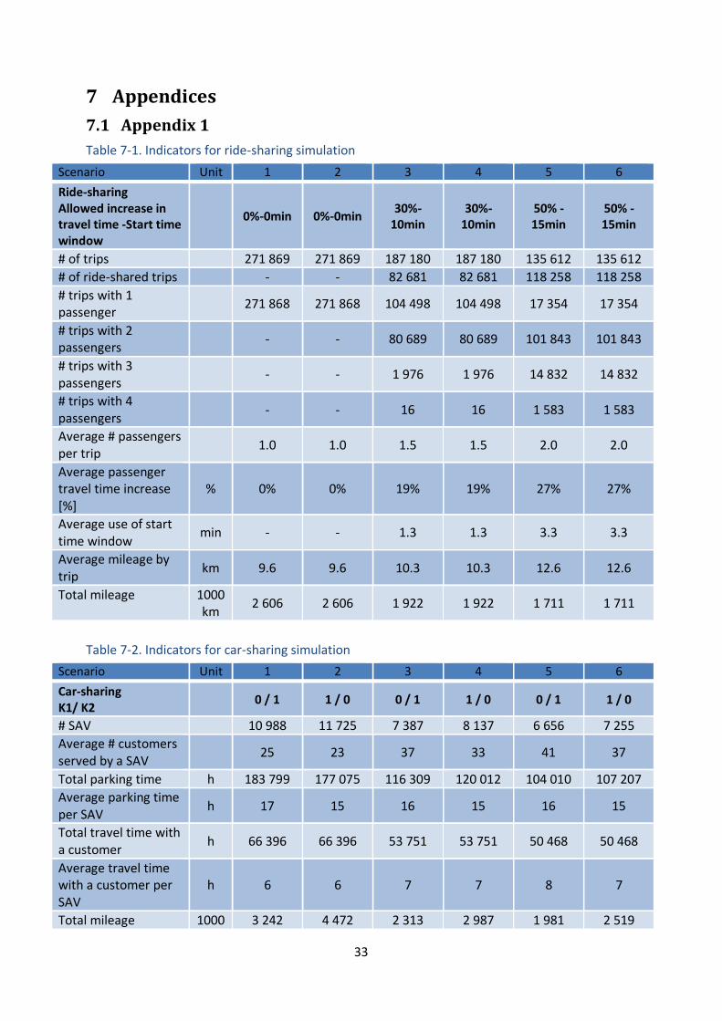
33

7 Appendices

7.1 Appendix 1

Table 7-1. Indicators for ride-sharing simulation

Scenario Unit 1 2 3 4 5 6

Ride-sharing Allowed increase in travel time -Start time window

0%-0min 0%-0min 30%-

10min 30%-

10min 50% - 15min

50% - 15min

# of trips 271 869 271 869 187 180 187 180 135 612 135 612

# of ride-shared trips - - 82 681 82 681 118 258 118 258

# trips with 1 passenger

271 868 271 868 104 498 104 498 17 354 17 354

# trips with 2 passengers

- - 80 689 80 689 101 843 101 843

# trips with 3 passengers

- - 1 976 1 976 14 832 14 832

# trips with 4 passengers

- - 16 16 1 583 1 583

Average # passengers per trip

1.0 1.0 1.5 1.5 2.0 2.0

Average passenger travel time increase [%]

% 0% 0% 19% 19% 27% 27%

Average use of start time window

min - - 1.3 1.3 3.3 3.3

Average mileage by trip

km 9.6 9.6 10.3 10.3 12.6 12.6

Total mileage 1000 km

2 606 2 606 1 922 1 922 1 711 1 711

Table 7-2. Indicators for car-sharing simulation

Scenario Unit 1 2 3 4 5 6

Car-sharing K1/ K2

0 / 1 1 / 0 0 / 1 1 / 0 0 / 1 1 / 0

# SAV 10 988 11 725 7 387 8 137 6 656 7 255

Average # customers served by a SAV

25 23 37 33 41 37

Total parking time h 183 799 177 075 116 309 120 012 104 010 107 207

Average parking time per SAV

h 17 15 16 15 16 15

Total travel time with a customer

h 66 396 66 396 53 751 53 751 50 468 50 468

Average travel time with a customer per SAV

h 6 6 7 7 8 7

Total mileage 1000 3 242 4 472 2 313 2 987 1 981 2 519

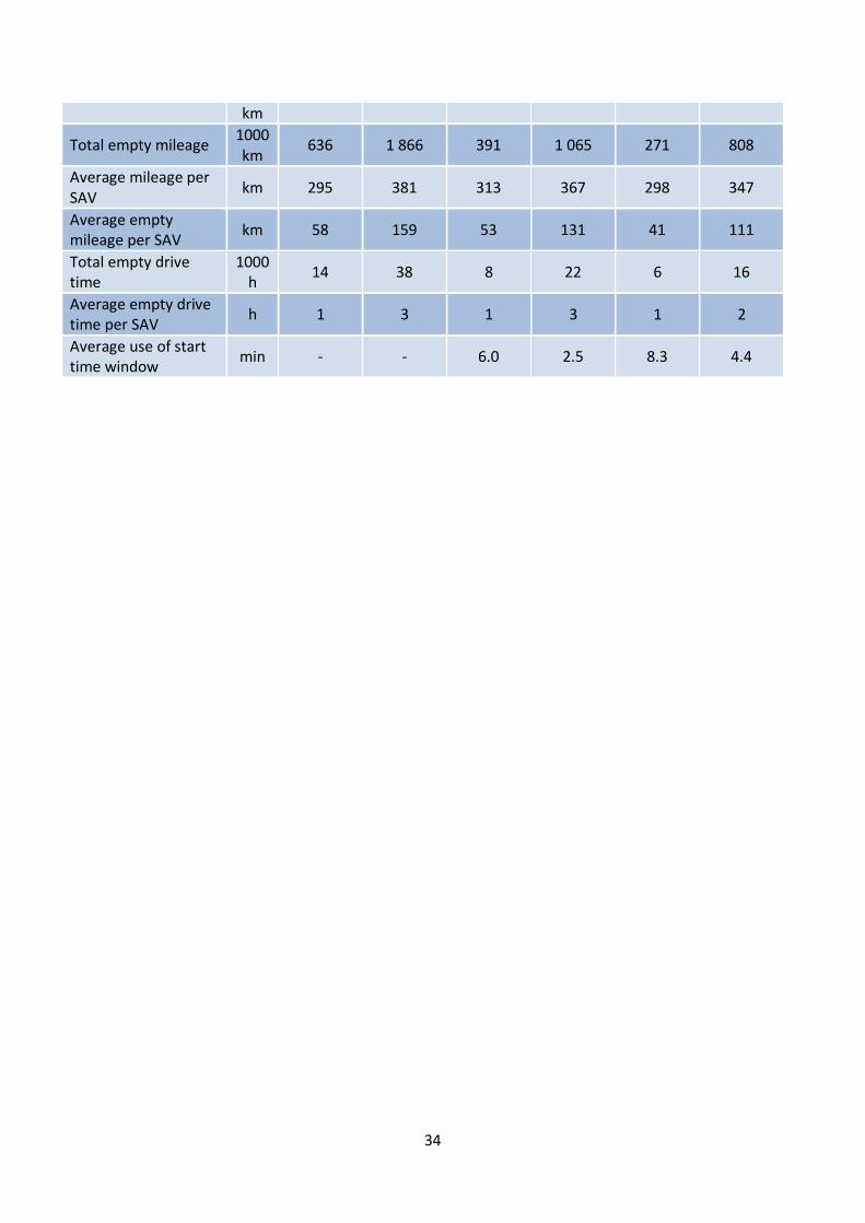
34

km

Total empty mileage 1000 km

636 1 866 391 1 065 271 808

Average mileage per SAV

km 295 381 313 367 298 347

Average empty mileage per SAV

km 58 159 53 131 41 111

Total empty drive time

1000 h

14 38 8 22 6 16

Average empty drive time per SAV

h 1 3 1 3 1 2

Average use of start time window

min - - 6.0 2.5 8.3 4.4