Study of Drug Assimilation in Human System using Physics

1

Study of Drug Assimilation in Human System using Physics

Informed Neural Networks

Kanupriya Goswami

Department of Physics

Keshav Mahavidyalaya

University of Delhi

Delhi, India

kanupriyagoswami@keshav.

du.ac.in

Arpana Sharma

Department of Mathematics


University of Delhi

Delhi, India

[email protected]

Madhu Pruthi

Department of Microbiology


University of Delhi

Delhi, India

[email protected]

Richa Gupta

Department of

Computer Science

University of Delhi

Delhi, India

[email protected]

m

Abstract:

Differential equations play a pivotal role in modern world ranging from science, engineering,

ecology, economics and finance where these can be used to model many physical systems and

processes. In this paper, we study two mathematical models of a drug assimilation in the human

system using Physics Informed Neural Networks (PINNs). In the first model, we consider the

case of single dose of drug in the human system and in the second case, we consider the course

of this drug taken at regular intervals. We have used the compartment diagram to model these

cases. The resulting differential equations are solved using PINN, where we employ a feed

forward multilayer perceptron as function approximator and the network parameters are tuned

for minimum error. Further, the network is trained by finding the gradient of the error function

with respect to the network parameters. We have employed DeepXDE, a python library for

PINNs, to solve the simultaneous first order differential equations describing the two models

of drug assimilation. The results show high degree of accuracy between the exact solution and

the predicted solution as much as the resulting error reaches10−11 for the first model and 10−8

for the second model. This validates the use of PINN in solving any dynamical system.

Keywords- Physics Informed Neural networks (PINNs), Pharmacokinetics, Drug Assimilation,

Compartment Model, Simultaneous Differential Equations, Neural Networks.

Introduction:

Differential equations (DEs) play a significant role in describing the behaviour of dynamical

systems in real world problems. Since the time rate change of any function is represented by

derivatives, such dynamical systems can be modelled by DEs. The exact solution of a DEs may

not be always possible and are solved by finite-differencing methods such as Euler, Modified

Euler or Runge-Kutta methods. Though these methods are efficient but require much memory

space and time. Neural Networks (NNs) provide an alternative way to solve DEs by acting as

function approximator and predict the solution in closed analytical form. The idea of solving

Ordinary Differential Equations (ODEs) and Partial Differential Equations (PDEs) using a NN

was described by Lagaris et al [ 1]. The concept used by Lagaris et al was to train a NN to satisfy

the conditions necessary for a differential equation. This acted as an impetus for researchers and

several models of NNs are being applied to solve DEs using neural networks [ 1-10].

Recently deep learning has emerged as a powerful tool in machine learning research under the

name Scientific Machine Learning. Deep learning, which involves the use of deep neural

networks has incredible ability and flexibility to solve many complex and high dimensional

problems as compared to the traditional approaches. Deep Learning is extensively used to solve

many problems in different domains of physical sciences. Deep neural networks have a

2

remarkable property of being universal function approximators, and can be used to predict the

solutions of ODEs and PDEs [11-17]. The fundamental step in solving a DE using deep

learning is to restrict a NN for minimum DE residual. The model consists of feedforward

network with an input layer, an output layer, multiple hidden layers and the nodes in the

adjacent layer being interconnected. Over the last few years, much research has been carried

out which elucidates the application of deep neural networks to solve different kinds of

differential equations as linear, non-linear, simultaneous, coupled, elliptical, fractional and

many other complex differential equations [11-17]. Recently, PINNs have been used by many

researchers to solve many types of DEs [18-21]. A PINN incorporates the physical laws of any

given physical system by satisfying its boundary conditions and initial conditions in the loss

function.

In the present study, we make us of the method of PINN proposed by Raissi et al. [11] to

study the drug assimilation in human system. Here, we use Deep XDE [13], a python library

for physics informed neural networks (PINNs), to solve the simultaneous first order differential

equations describing the two models of drug assimilation in human body. DeepXDE is an

evolving python library which is being used to solve Multiphysics problems. The library

supports complex geometry domain and the user code remains concise and adaptable to the

problem concerned.

The mathematics of pharmacokinetics deals with the rate of assimilation, distribution and

elimination of the drugs by the human system over a period of time. Mathematical Modelling

in this field establishes the realistic conclusions and helps to understand efficacy and

therapeutic response of any drug in the human body. The Compartment model is used to study

the process of drug assimilation, where the human body is represented as a sequence of

compartments. The number of compartments in this model depends upon the nature and

behaviour of drug being considered. We consider a three compartment model, where the human

body is characterized by three separate compartments i.e. the gastrointestinal tract (GI-tract),

the bloodstream and the urinary tract. We further consider the urinary tract as an absorbing

compartment only i.e. the drug enters but is not eliminated from the urinary tract. The goal of

this mathematical model of drug assimilation in blood is to see how these drugs are absorbed

into the human, which would be valuable in assessing the therapeutic value of a drug . The

different drugs are absorbed and eliminated at different rates. The drug is first absorbed in the

gastrointestinal tract (GI-tract) and then is diffused into the bloodstream. The drug is then

carried to the location where the therapeutic effect is desired and finally is eliminated from the

bloodstream by the kidneys and liver to the urinary tract. The absorption and elimination of

the drug may occur at different rates for the different constituents of the same drug.

One of the earliest compartment model was given by Widmark [22], who developed an open

one compartment model to study the blood alcohol concentration and is still used in forensic

research. Spitznagel Edward [23] also presented a two compartment pharmacokinetics model.

Koch [24] described biomathematical modelling in pharmacokinetics by using one and two

compartment models to study the single and multiple injection models. Khanday et al [25]

established the mathematical model to estimate the drug distribution in blood and tissue using

oral and intravenous methods and resulting DEs were solved using Laplace transform and

eigenvalue method. Egbelowo [26] considered non-standard finite difference method to solve

one compartment pharmacokinetic model for different routes of drug administration.

In this paper, we apply Deep learning using PINN to study the assimilation of drug using three

compartment model. Further we take up two models -First, the case of single dose of drug and

3

second, the case of regular dosage of drug. The model and the constants have been taken from

Belinda et al [27].

Mathematical Formulation:

In this section, we begin with a brief description of physics-informed neural networks (PINNs)

[11] that incorporates physical laws, PINN algorithm and workflow implementation of

DeepXDE to simultaneous DEs describing drug assimilation models. The PINNs embed a DE

into the loss using automatic differentiation and training is implemented by integrating the data

and physical laws. This approach which is mesh free compared to other traditional approaches

can be used to solve forward and inverse problems.

We consider the following form of DE defined in equation (1) and (2) on the domain Ω, with

the boundary dΩ.

ℱ(u(t)) = 0 t ∈ Ω (1)

𝒢(u(t)) = 0 t ∈ dΩ (2)

Where, u is the unknown function of variable t to be determined and ℱ is a differential operator

that may be linear or non-linear. The operator 𝒢 denotes the boundary conditions of the given

differential equation (1). Since our differential equation contains temporal variable t, it is

included in the domain Ω and the initial condition is treated as special type of Dirichlet

boundary condition.

Let �̂� (𝑡; 𝜃) be the NN, which approximates the solution u(t) of our differential equation and

takes t as input. Figure 1 shows the network consisting of an input layer, five hidden layers and

an output layer. The network parameter 𝜃 = {𝜔𝑘 , 𝑏𝑘} is the collection of the weight matrix

(𝜔𝑘) and bias vector (𝑏𝑘) for each layer. These network parameters are continuously optimized

during training process and automatic differentiation is used to calculate the derivative of �̂�

with respect t. To satisfy the conditions of physical laws in the differential equation, we define

a residual network by equation (3):

𝑓(𝑡; 𝜃) ∶= Ν[�̂� (𝑡; 𝜃)] (3)

The network can be trained by minimizing the loss function. The loss function for the PINN is

given in equation (4) [11]:

ℒ(𝜃) = 𝑀𝑆𝐸𝑓 + 𝑀𝑆𝐸𝑏 (4)

where, the Mean Square Error (MSE) is given by the following equations (5) and (6):

𝑀𝑆𝐸𝑓 = 1

𝑇𝑓 ∑|𝑓(𝑡𝑓

𝑖 )|2

𝑇𝑓

𝑖=1

(5)

𝑀𝑆𝐸𝑏 = 1

𝑇𝑏 ∑|𝑢�̂� − 𝑢(𝑡𝑏

𝑖 )|2

𝑇𝑏

𝑖=1

(6)

4

where, 𝑇𝑏 and 𝑇𝑓 are the points on the boundary and on the domain respectively, and together

they constitute the training data 𝑇 = {𝑡1, 𝑡2, 𝑡3, … . . 𝑡|𝑇| } of size |𝑇|. Here 𝑢(𝑡𝑏𝑖 ) denotes the

training data from the initial conditions. The next step is to minimize the loss ℒ(𝜃), called the

training process, which is performed by using the gradient based optimizers. In our study, we

have used Adam and BFGS optimizers. The above-mentioned process leads to a trained NN,

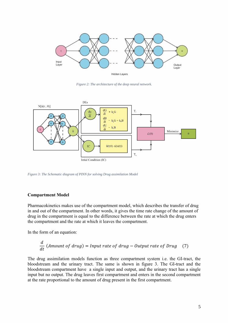
which approximates the solution of our differential equations. The Schematic diagram of PINN

for drug assimilation model is shown in figure 2. The figure 1 presents the work flow

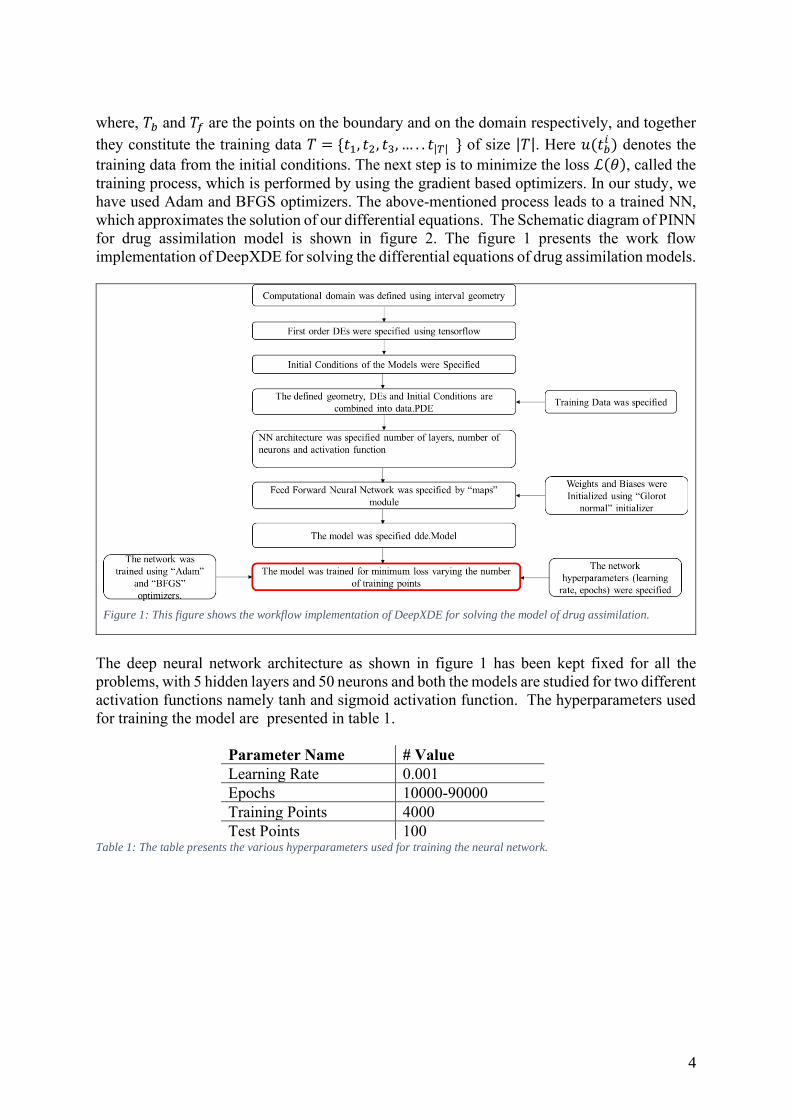
implementation of DeepXDE for solving the differential equations of drug assimilation models.

Figure 1: This figure shows the workflow implementation of DeepXDE for solving the model of drug assimilation.

The deep neural network architecture as shown in figure 1 has been kept fixed for all the

problems, with 5 hidden layers and 50 neurons and both the models are studied for two different

activation functions namely tanh and sigmoid activation function. The hyperparameters used

for training the model are presented in table 1.

Parameter Name # Value

Learning Rate 0.001

Epochs 10000-90000

Training Points 4000

Test Points 100 Table 1: The table presents the various hyperparameters used for training the neural network.

5

Figure 2: The architecture of the deep neural network.

Figure 3: The Schematic diagram of PINN for solving Drug assimilation Model

Compartment Model

Pharmacokinetics makes use of the compartment model, which describes the transfer of drug

in and out of the compartment. In other words, it gives the time rate change of the amount of

drug in the compartment is equal to the difference between the rate at which the drug enters

the compartment and the rate at which it leaves the compartment.

In the form of an equation:

𝑑

𝑑𝑡 (𝐴𝑚𝑜𝑢𝑛𝑡 𝑜𝑓 𝑑𝑟𝑢𝑔) = 𝐼𝑛𝑝𝑢𝑡 𝑟𝑎𝑡𝑒 𝑜𝑓 𝑑𝑟𝑢𝑔 − 𝑂𝑢𝑡𝑝𝑢𝑡 𝑟𝑎𝑡𝑒 𝑜𝑓 𝐷𝑟𝑢𝑔 (7)

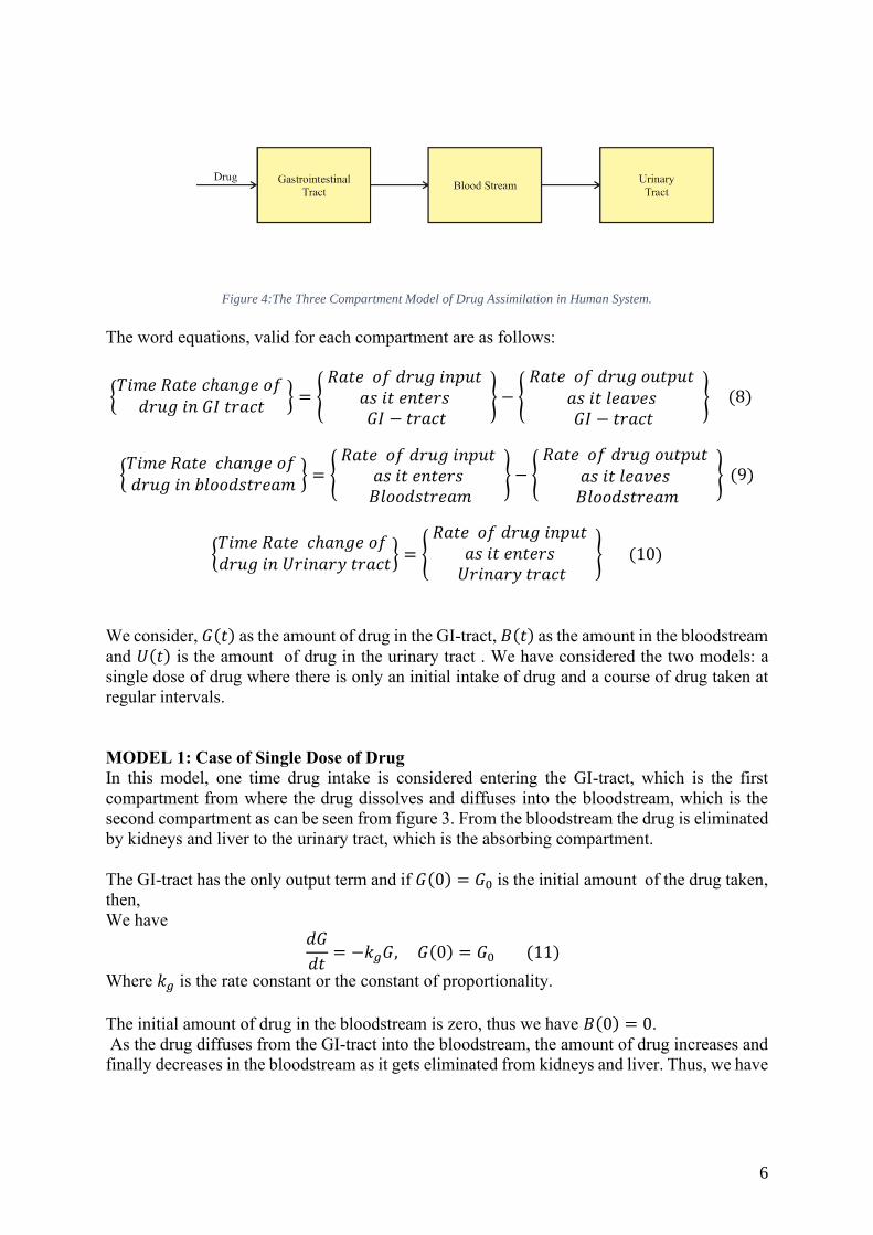
The drug assimilation models function as three compartment system i.e. the GI-tract, the

bloodstream and the urinary tract. The same is shown in figure 3. The GI-tract and the

bloodstream compartment have a single input and output, and the urinary tract has a single

input but no output. The drug leaves first compartment and enters in the second compartment

at the rate proportional to the amount of drug present in the first compartment.

6

Figure 4:The Three Compartment Model of Drug Assimilation in Human System.

The word equations, valid for each compartment are as follows:

{𝑇𝑖𝑚𝑒 𝑅𝑎𝑡𝑒 𝑐ℎ𝑎𝑛𝑔𝑒 𝑜𝑓

𝑑𝑟𝑢𝑔 𝑖𝑛 𝐺𝐼 𝑡𝑟𝑎𝑐𝑡} = {

𝑅𝑎𝑡𝑒 𝑜𝑓 𝑑𝑟𝑢𝑔 𝑖𝑛𝑝𝑢𝑡 𝑎𝑠 𝑖𝑡 𝑒𝑛𝑡𝑒𝑟𝑠 𝐺𝐼 − 𝑡𝑟𝑎𝑐𝑡

} − { 𝑅𝑎𝑡𝑒 𝑜𝑓 𝑑𝑟𝑢𝑔 𝑜𝑢𝑡𝑝𝑢𝑡

𝑎𝑠 𝑖𝑡 𝑙𝑒𝑎𝑣𝑒𝑠 𝐺𝐼 − 𝑡𝑟𝑎𝑐𝑡

} (8)

{𝑇𝑖𝑚𝑒 𝑅𝑎𝑡𝑒 𝑐ℎ𝑎𝑛𝑔𝑒 𝑜𝑓 𝑑𝑟𝑢𝑔 𝑖𝑛 𝑏𝑙𝑜𝑜𝑑𝑠𝑡𝑟𝑒𝑎𝑚

} = { 𝑅𝑎𝑡𝑒 𝑜𝑓 𝑑𝑟𝑢𝑔 𝑖𝑛𝑝𝑢𝑡

𝑎𝑠 𝑖𝑡 𝑒𝑛𝑡𝑒𝑟𝑠 𝐵𝑙𝑜𝑜𝑑𝑠𝑡𝑟𝑒𝑎𝑚

} − { 𝑅𝑎𝑡𝑒 𝑜𝑓 𝑑𝑟𝑢𝑔 𝑜𝑢𝑡𝑝𝑢𝑡

𝑎𝑠 𝑖𝑡 𝑙𝑒𝑎𝑣𝑒𝑠 𝐵𝑙𝑜𝑜𝑑𝑠𝑡𝑟𝑒𝑎𝑚

} (9)

{𝑇𝑖𝑚𝑒 𝑅𝑎𝑡𝑒 𝑐ℎ𝑎𝑛𝑔𝑒 𝑜𝑓 𝑑𝑟𝑢𝑔 𝑖𝑛 𝑈𝑟𝑖𝑛𝑎𝑟𝑦 𝑡𝑟𝑎𝑐𝑡

} = { 𝑅𝑎𝑡𝑒 𝑜𝑓 𝑑𝑟𝑢𝑔 𝑖𝑛𝑝𝑢𝑡

𝑎𝑠 𝑖𝑡 𝑒𝑛𝑡𝑒𝑟𝑠 𝑈𝑟𝑖𝑛𝑎𝑟𝑦 𝑡𝑟𝑎𝑐𝑡

} (10)

We consider, 𝐺(𝑡) as the amount of drug in the GI-tract, 𝐵(𝑡) as the amount in the bloodstream

and 𝑈(𝑡) is the amount of drug in the urinary tract . We have considered the two models: a

single dose of drug where there is only an initial intake of drug and a course of drug taken at

regular intervals.

MODEL 1: Case of Single Dose of Drug

In this model, one time drug intake is considered entering the GI-tract, which is the first

compartment from where the drug dissolves and diffuses into the bloodstream, which is the

second compartment as can be seen from figure 3. From the bloodstream the drug is eliminated

by kidneys and liver to the urinary tract, which is the absorbing compartment.

The GI-tract has the only output term and if 𝐺(0) = 𝐺0 is the initial amount of the drug taken,

then,

We have 𝑑𝐺

𝑑𝑡= −𝑘𝑔𝐺, 𝐺(0) = 𝐺0 (11)

Where 𝑘𝑔 is the rate constant or the constant of proportionality.

The initial amount of drug in the bloodstream is zero, thus we have 𝐵(0) = 0.

As the drug diffuses from the GI-tract into the bloodstream, the amount of drug increases and

finally decreases in the bloodstream as it gets eliminated from kidneys and liver. Thus, we have

7

𝑑𝐵

𝑑𝑡= 𝑘𝑔𝐺 − 𝑘𝑏𝐵, 𝐵(0) = 0 (12)

Where 𝑘𝑏 is the another rate constant or the constant of proportionality.

Since the drug enters the urinary tract and is not eliminated from the urinary tract, the equation

describing this behaviour can be written as

𝑑𝑈

𝑑𝑡= 𝑘𝑏𝐵, 𝑈(0) = 0 (13)

Where 𝑈(0) = 0, is the initial amount of the drug in the urinary tract.

Thus the three compartment model, which describes the rate of change of drug as it diffuses

through the human system is given by the equations (11), (12) and (13).

The values of the rates at which the drug diffuses from the GI-tract into the bloodstream and

then is eliminated, are 0.72 ℎ𝑜𝑢𝑟−1 and 0.15 ℎ𝑜𝑢𝑟−1respectively. The initial amount of the

drug in GI-tract is 0.0001 milligrams. The values of the coefficients have been taken from

Belinda et al [27], where the drug considered is antibiotic tetracycline.

Results & discussions for Model 1:

The network for this model has been trained for two activation functions, namely, tanh and

sigmoid. The number of epochs have been varied from 10000 to 90000 and the loss is

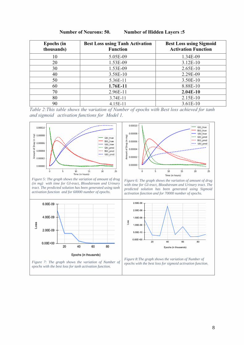
minimized. Table 2 shows the variation of number of epochs with best loss achieved for the

two activation functions considered. The best loss of 1.76E-11 in the case of tanh activation

function is obtained for 60000 epochs. The best loss of 2.04E-10 in the case of Sigmoid

activation function is obtained for 70000 epochs. We have plotted graphs comparing the exact

and predicted solutions for the case of best loss for both the activation functions. The graph in

the figure 4 presents the variation of amount of drug in GI-tract, bloodstream and urinary tract

with time using tanh activation function for the 60000 number of epochs. The graph in the

figure 5 presents the variation of concentrations of drug in GI-tract, bloodstream and urinary

tract with time using sigmoid activation function for 70000 number of epochs. The variations

have been studied for a period of 24 hours and show good convergence between predicted and

exact solutions for GI-tract and bloodstream for both the activation functions. The convergence

of exact and predicted solutions for urinary tract is better for tanh activation function as

compared to sigmoid activation function.

The graphs in the figures 5 & 6 show that as time passes, the amount of drug in GI-tract

decreases and approaches zero for both the activation functions. The amount of drug in the

bloodstream initially increases with time and then approaches zero. The peak as observed in

the bloodstream shows the effectiveness of the drug, as can be seen, will be approximately

after 3 hours. The behaviour of the drug depends on the coefficients 𝑘𝑔 and 𝑘𝑏 associated with

each drug. These coefficients depend on the condition and well-being of the patients concerned,

which means the peak for the drug for some patients will show different behaviour than for

an average person. The graph in the figure 7 & 8 shows the variation of number of epochs with

the best loss for tanh and sigmoid activation function. The graph for tanh activation in figure

7 shows that the loss decreases as the number of epochs increases and reaches an order of

10−11 at 50000 epochs. The graph for sigmoid activation function in figure 8 shows that

though the order of loss achieved is 10−10 , it shows fluctuations.

8

Number of Neurons: 50. Number of Hidden Layers :5

Epochs (in

thousands)

Best Loss using Tanh Activation

Function

Best Loss using Sigmoid

Activation Function

10 5.05E-09 1.34E-09

20 1.53E-09 3.12E-10

30 1.53E-09 2.65E-10

40 3.58E-10 2.29E-09

50 5.36E-11 3.50E-10

60 1.76E-11 8.88E-10

70 2.96E-11 2.04E-10

80 3.74E-11 2.15E-10

90 4.15E-11 3.61E-10

Table 2:This table shows the variation of Number of epochs with Best loss achieved for tanh

and sigmoid activation functions for Model 1.

Figure 5: The graph shows the variation of amount of drug

(in mg) with time for GI-tract, Bloodstream and Urinary

tract. The predicted solution has been generated using tanh

activation function and for 60000 number of epochs.


with time for GI-tract, Bloodstream and Urinary tract. The

predicted solution has been generated using Sigmoid


Figure 7: The graph shows the variation of Number of

epochs with the best loss for tanh activation function.

Figure 8:The graph shows the variation of Number of

epochs with the best loss for sigmoid activation function.

9

MODEL 2: Case of Regular Dose of Drug

In this model the drug is taken at regular intervals, which makes a continuous inflow of drug

in GI-tract. Let 𝑓 be a positive constant which represents the rate of intake of the drug.

Further, we consider two cases-First when 𝑓 is a positive constant function and second, when

𝑓 is a pulsing function i.e. 𝑓(𝑡), representing repeated doses.

The mathematical equations describing the time rate change of amount of drug in this case are

given by equations (14-16)

𝑑𝐺

𝑑𝑡= 𝑓 − 𝑘𝑔𝐺, 𝐺(0) = 0 (14)

𝑑𝐵

𝑑𝑡= 𝑘𝑔𝐺 − 𝑘𝑏𝐵, 𝐵(0) = 0 (15)

𝑑𝑈

𝑑𝑡= 𝑘𝑏𝐵, 𝑈(0) = 0 (16)

Case 1: When 𝑓 be a positive constant

In this case, the drug is taken 1 unit per hour and there is a regular intake of drug in the GI-

tract. We further assume that the constant 𝑓 for this drug dissolves at constant rate, which

implies that the drug gets released slowly and evenly over a period of time.

Case 2: When 𝑓 is a pulsing function

In this case, we have considered that the drug gets dissolved quickly and thus the function 𝑓 is

a pulsing function of the form 𝑓(𝑡) = 1 + cos𝜋 𝑡

12 .

Results & discussions for Model 2:

Case 1: when 𝒇 be a positive constant

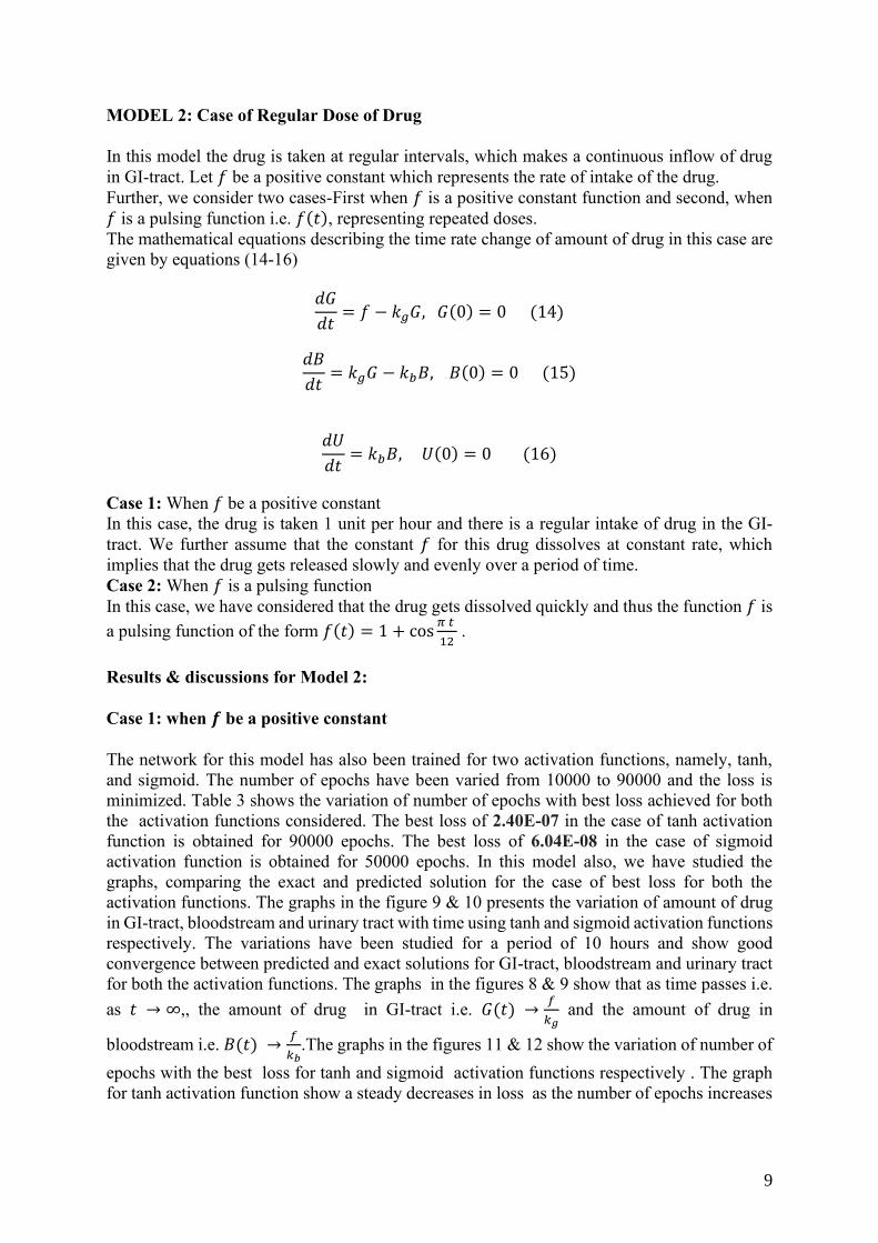
The network for this model has also been trained for two activation functions, namely, tanh,

and sigmoid. The number of epochs have been varied from 10000 to 90000 and the loss is

minimized. Table 3 shows the variation of number of epochs with best loss achieved for both

the activation functions considered. The best loss of 2.40E-07 in the case of tanh activation

function is obtained for 90000 epochs. The best loss of 6.04E-08 in the case of sigmoid

activation function is obtained for 50000 epochs. In this model also, we have studied the

graphs, comparing the exact and predicted solution for the case of best loss for both the

activation functions. The graphs in the figure 9 & 10 presents the variation of amount of drug

in GI-tract, bloodstream and urinary tract with time using tanh and sigmoid activation functions

respectively. The variations have been studied for a period of 10 hours and show good

convergence between predicted and exact solutions for GI-tract, bloodstream and urinary tract

for both the activation functions. The graphs in the figures 8 & 9 show that as time passes i.e.

as 𝑡 → ∞,, the amount of drug in GI-tract i.e. 𝐺(𝑡) →𝑓

𝑘𝑔 and the amount of drug in

bloodstream i.e. 𝐵(𝑡) →𝑓

𝑘𝑏.The graphs in the figures 11 & 12 show the variation of number of

epochs with the best loss for tanh and sigmoid activation functions respectively . The graph

for tanh activation function show a steady decreases in loss as the number of epochs increases

10

and reaches an order of 10-7 for 50000 epochs. The graph for sigmoid activation function

reaches an order of 10-8 for 50000 epochs and then shows minor fluctuations.

Number of Neurons: 50. Number of Hidden Layers : 5

Epochs (in thousands) Best loss using Tanh Activation

Function

Best loss using Sigmoid

Activation Function

10 3.01E-06 7.67E-07

20 1.77E-06 2.78E-07

30 1.66E-06 2.27E-07

40 1.16E-06 1.11E-07

50 5.43E-07 6.04E-08

60 2.51E-07 8.23E-08

70 3.60E-07 8.86E-08

80 3.51E-07 7.78E-08

90 2.40E-07 8.64E-08

Table 3: This table shows the variation of Number of epochs with Best loss achieved for tanh

and sigmoid activation functions for Model 2 when 𝑓 is a positive constant.


(in mg) with time for GI-tract, Bloodstream and Urinary

tract. The predicted solution has been generated using

tanh activation function and for 90000 number of epochs.

Figure 10: The graph shows the variation of amount of

drug with time for GI-tract, Bloodstream and Urinary

tract. The predicted solution has been generated using

Sigmoid activation function and 50000 number of epochs.

Figure 11: The graph shows. the variation of Number of

epochs with the best loss for tanh activation function.

Figure 12:Figure 10: The graph shows. the variation of

Number of epochs with the best loss for sigmoid activation

function.

11

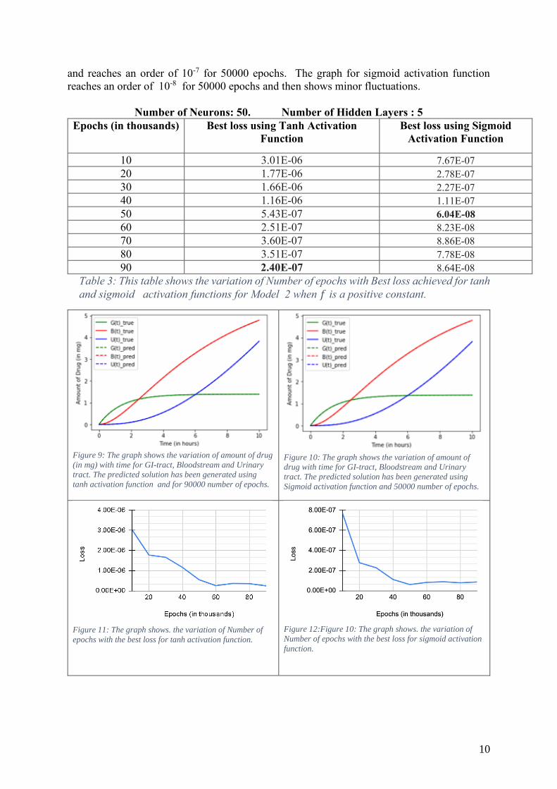
Case 2: When 𝒇 is a pulsing function

In this case, we have considered that the drug gets dissolved very quickly and hence the

function 𝑓 should be a pulsing function of the form 𝑓(𝑡) = 1 + cos𝜋 𝑡

12 representing repeated

dosage. Table 4 presents the variation of number of epochs with best loss achieved for both the

activation functions considered. The best loss of 8.78E-07 in the case of tanh activation

function is obtained for 80000 epochs. The best loss of 4.11E-07in the case of sigmoid

activation function is obtained for 90000 epochs. The graphs in the figure 13 & 14 presents the

variation of amount of drug in GI-tract and bloodstream with time using tanh and sigmoid

activation functions respectively. These graphs shows the comparison of the predicted and

exact solution for best loss achieved in respective activation functions. As can be seen from

both the figures that, when 𝑓 is a pulsing function, there is an initial and significant increase in

the drug amount and subsequently very less during the residual period before the next dose is

taken. The variations show excellent convergence between predicted and exact solutions, for

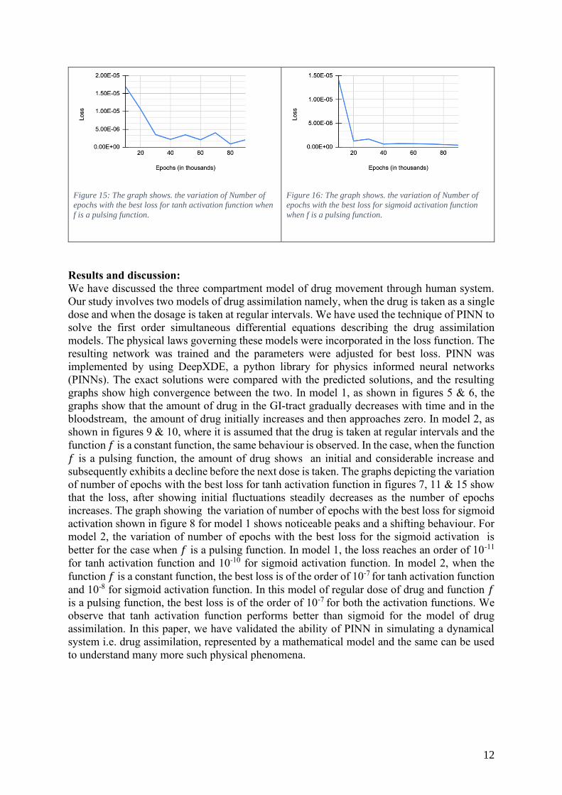
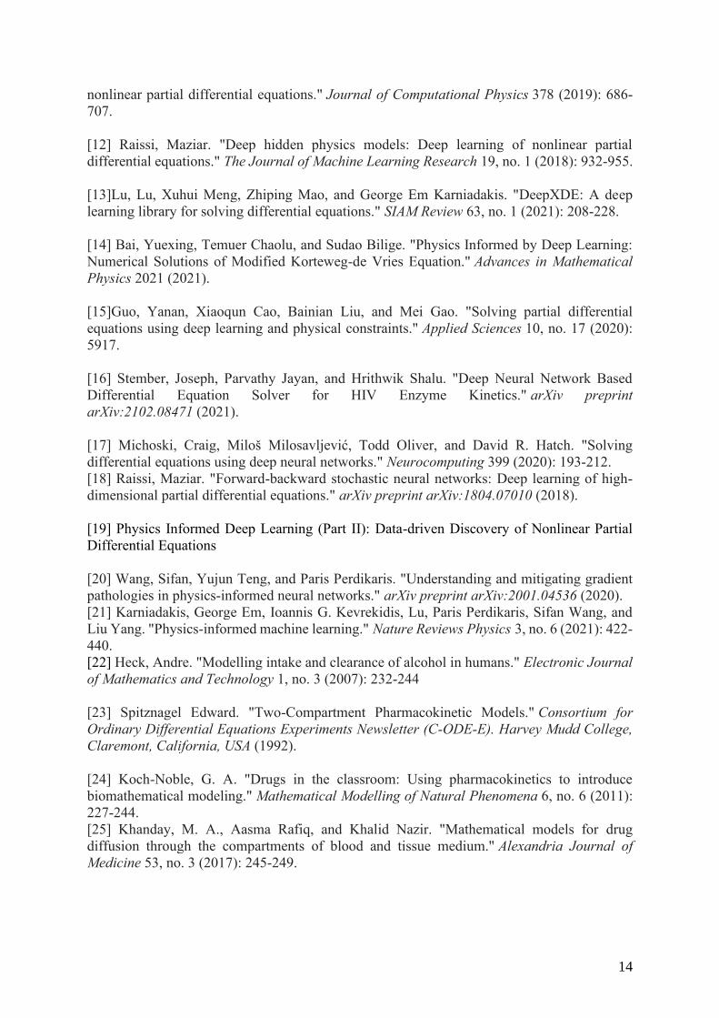
both the activation functions. The figures 15 & 16 show the variation of best loss and number

of epochs for tanh and sigmoid activation function. The best loss is of the order of 10−7for

both the activation functions. The loss fluctuates for tanh activation function, but steadily

decreases for sigmoid after 50000 epochs.

Number of Neurons: 50. Number of Hidden Layers : 5

Epochs (in thousands) Best loss using Tanh Activation

Function

Best loss using Sigmoid

Activation Function

10 1.69E-05 1.41E-05

20 1.06E-05 1.28E-06

30 3.50E-06 1.68E-06

40 2.17E-06 6.36E-07

50 3.44E-06 7.39E-07

60 2.05E-06 7.14E-07

70 4.01E-06 6.42E-07

80 8.78E-07 5.30E-07

90 2.02E-06 4.11E-07 Table 4:This table shows the variation of Number of epochs with Best loss achieved for tanh and sigmoid activation

functions for Model 2 when f is a pulsing function given by 𝑓(𝑡) = 1 + 𝑐𝑜𝑠𝜋 𝑡

12 .


drug (in mg) with time for GI-tract, Bloodstream. The

predicted solution has been generated using tanh



drug (in mg) with time for GI-tract, Bloodstream. The

predicted solution has been generated using Sigmoid

activation function and 90000 number of epochs.

12


epochs with the best loss for tanh activation function when

f is a pulsing function.


epochs with the best loss for sigmoid activation function

when f is a pulsing function.

Results and discussion:

We have discussed the three compartment model of drug movement through human system.

Our study involves two models of drug assimilation namely, when the drug is taken as a single

dose and when the dosage is taken at regular intervals. We have used the technique of PINN to

solve the first order simultaneous differential equations describing the drug assimilation

models. The physical laws governing these models were incorporated in the loss function. The

resulting network was trained and the parameters were adjusted for best loss. PINN was

implemented by using DeepXDE, a python library for physics informed neural networks

(PINNs). The exact solutions were compared with the predicted solutions, and the resulting

graphs show high convergence between the two. In model 1, as shown in figures 5 & 6, the

graphs show that the amount of drug in the GI-tract gradually decreases with time and in the

bloodstream, the amount of drug initially increases and then approaches zero. In model 2, as

shown in figures 9 & 10, where it is assumed that the drug is taken at regular intervals and the

function 𝑓 is a constant function, the same behaviour is observed. In the case, when the function

𝑓 is a pulsing function, the amount of drug shows an initial and considerable increase and

subsequently exhibits a decline before the next dose is taken. The graphs depicting the variation

of number of epochs with the best loss for tanh activation function in figures 7, 11 & 15 show

that the loss, after showing initial fluctuations steadily decreases as the number of epochs

increases. The graph showing the variation of number of epochs with the best loss for sigmoid

activation shown in figure 8 for model 1 shows noticeable peaks and a shifting behaviour. For

model 2, the variation of number of epochs with the best loss for the sigmoid activation is

better for the case when 𝑓 is a pulsing function. In model 1, the loss reaches an order of 10-11

for tanh activation function and 10-10 for sigmoid activation function. In model 2, when the

function 𝑓 is a constant function, the best loss is of the order of 10-7 for tanh activation function

and 10-8 for sigmoid activation function. In this model of regular dose of drug and function 𝑓

is a pulsing function, the best loss is of the order of 10-7 for both the activation functions. We

observe that tanh activation function performs better than sigmoid for the model of drug

assimilation. In this paper, we have validated the ability of PINN in simulating a dynamical

system i.e. drug assimilation, represented by a mathematical model and the same can be used

to understand many more such physical phenomena.

13

Conclusions:

In this work, we employ Deep Learning using physics informed neural networks technique to

solve the three compartment model of drug assimilation in human system. We see high

convergence in the exact and predicted solutions for tanh activation function for both the

models. The work further elucidates and validates the efficacy and flexibility of PINNs to

solve first order simultaneous differential equations representing the model of drug

assimilation in human system. In. future, we hope to use PINNs to model many other physical

systems defined by ODEs and PDEs.

References:

[1 ] Lagaris, Isaac E., Aristidis Likas, and Dimitrios I. Fotiadis. "Artificial neural networks for

solving ordinary and partial differential equations." IEEE transactions on neural networks 9,

no. 5 (1998): 987-1000.

[2] Lagaris, Isaac E., Aristidis C. Likas, and Dimitris G. Papageorgiou. "Neural-network

methods for boundary value problems with irregular boundaries." IEEE Transactions on

Neural Networks 11, no. 5 (2000): 1041-1049.

[3 ] Dockhorn, Tim. "A discussion on solving partial differential equations using neural

networks." arXiv preprint arXiv:1904.07200 (2019).

[4] Hayati, Mohsen, and Behnam Karami. "Feedforward neural network for solving partial

differential equations." Journal of Applied Sciences 7, no. 19 (2007): 2812-2817.

[5 ] Liu, Zeyu, Yantao Yang, and Qingdong Cai. "Neural network as a function approximator

and its application in solving differential equations." Applied Mathematics and Mechanics 40,

no. 2 (2019): 237-248

[6] Meade Jr, Andrew J., and Alvaro A. Fernandez. "The numerical solution of linear ordinary

differential equations by feedforward neural networks." Mathematical and Computer

Modelling 19, no. 12 (1994): 1-25

[7] Pratama, Danang Adi, Maharani Abu Bakar, Mustafa Man, and M. Mashuri. "ANNs-Based

Method for Solving Partial Differential Equations: A Survey." (2021)

[8] Chiaramonte, M., and M. Kiener. "Solving differential equations using neural

networks." Machine Learning Project 1 (2013)

[9] Guidetti, Veronica, Francesco Muia, Yvette Welling, and Alexander Westphal. "dNNsolve:

an efficient NN-based PDE solver." arXiv preprint arXiv:2103.08662 (2021).

[10] Baydin, A. G., Pearlmutter, B. A., Radul, A. A., & Siskind, J. M.. “Automatic

differentiation in machine learning: a survey” in Journal of machine learning research,

18(153), 2018.

[11] Raissi, Maziar, Paris Perdikaris, and George E. Karniadakis. "Physics-informed neural

networks: A deep learning framework for solving forward and inverse problems involving

14

nonlinear partial differential equations." Journal of Computational Physics 378 (2019): 686-

707.

[12] Raissi, Maziar. "Deep hidden physics models: Deep learning of nonlinear partial

differential equations." The Journal of Machine Learning Research 19, no. 1 (2018): 932-955.

[13]Lu, Lu, Xuhui Meng, Zhiping Mao, and George Em Karniadakis. "DeepXDE: A deep

learning library for solving differential equations." SIAM Review 63, no. 1 (2021): 208-228.

[14] Bai, Yuexing, Temuer Chaolu, and Sudao Bilige. "Physics Informed by Deep Learning:

Numerical Solutions of Modified Korteweg-de Vries Equation." Advances in Mathematical

Physics 2021 (2021).

[15]Guo, Yanan, Xiaoqun Cao, Bainian Liu, and Mei Gao. "Solving partial differential

equations using deep learning and physical constraints." Applied Sciences 10, no. 17 (2020):

5917.

[16] Stember, Joseph, Parvathy Jayan, and Hrithwik Shalu. "Deep Neural Network Based

Differential Equation Solver for HIV Enzyme Kinetics." arXiv preprint

arXiv:2102.08471 (2021).

[17] Michoski, Craig, Miloš Milosavljević, Todd Oliver, and David R. Hatch. "Solving

differential equations using deep neural networks." Neurocomputing 399 (2020): 193-212.

[18] Raissi, Maziar. "Forward-backward stochastic neural networks: Deep learning of high-

dimensional partial differential equations." arXiv preprint arXiv:1804.07010 (2018).

[19] Physics Informed Deep Learning (Part II): Data-driven Discovery of Nonlinear Partial

Differential Equations

[20] Wang, Sifan, Yujun Teng, and Paris Perdikaris. "Understanding and mitigating gradient

pathologies in physics-informed neural networks." arXiv preprint arXiv:2001.04536 (2020).

[21] Karniadakis, George Em, Ioannis G. Kevrekidis, Lu, Paris Perdikaris, Sifan Wang, and

Liu Yang. "Physics-informed machine learning." Nature Reviews Physics 3, no. 6 (2021): 422-

440.

[22] Heck, Andre. "Modelling intake and clearance of alcohol in humans." Electronic Journal

of Mathematics and Technology 1, no. 3 (2007): 232-244

[23] Spitznagel Edward. "Two-Compartment Pharmacokinetic Models." Consortium for

Ordinary Differential Equations Experiments Newsletter (C-ODE-E). Harvey Mudd College,

Claremont, California, USA (1992).

[24] Koch-Noble, G. A. "Drugs in the classroom: Using pharmacokinetics to introduce

biomathematical modeling." Mathematical Modelling of Natural Phenomena 6, no. 6 (2011):

227-244.

[25] Khanday, M. A., Aasma Rafiq, and Khalid Nazir. "Mathematical models for drug

diffusion through the compartments of blood and tissue medium." Alexandria Journal of

Medicine 53, no. 3 (2017): 245-249.

15

[26] Egbelowo Oluwaseun. "Nonlinear elimination of drugs in one-compartment

pharmacokinetic models: nonstandard finite difference approach for various routes of

administration." Mathematical and Computational Applications 23, no. 2 (2018): 27.

[27] Barnes, Belinda, and G. R. Fulford. Mathematical modelling with case studies: a

differential equations approach using Maple and MATLAB. Chapman and Hall/CRC, 2011.

Documents

Study of Drug Assimilation in Human System using Physics