Embed Size (px)
Citation preview
ERASMUS MUNDUS MSC PROGRAMME
COASTAL AND MARINE ENGINEERING AND MANAGEMENT
COMEM
STUDY OF FATIGUE DESIGN ON MARINE CURRENT TURBINE SUPPORT STRUCTURE
BALI - INDONESIA
UNIVERSITY OF SOUTHAMPTON
June 2011
Tubagus Ary Tresna Dirgantara
324496669
The Erasmus Mundus MSc Coastal and Marine Engineering and Management is an integrated
programme organized by five European partner institutions, coordinated by Delft University of
Technology (TU Delft). The joint study programme of 120 ECTS credits (two years full‐time) has been
obtained at three of the five CoMEM partner institutions:
• Norges Teknisk‐ Naturvitenskapelige Universitet (NTNU) Trondheim, Norway
• Technische Universiteit (TU) Delft, The Netherlands
• City University London, Great Britain
• Universitat Politècnica de Catalunya (UPC), Barcelona, Spain
• University of Southampton, Southampton, Great Britain
The first year consists of the first and second semesters of 30 ECTS each, spent at NTNU, Trondheim
and Delft University of Technology respectively.
The second year allows for specialization in three subjects and during the third semester courses are
taken with a focus on advanced topics in the selected area of specialization:
• Engineering
• Management
• Environment
In the fourth and final semester an MSc project and thesis have to be completed.
The two year CoMEM programme leads to three officially recognized MSc diploma certificates. These
will be issued by the three universities which have been attended by the student. The transcripts
issued with the MSc Diploma Certificate of each university include grades/marks for each subject. A
complete overview of subjects and ECTS credits is included in the Diploma Supplement, as received
from the CoMEM coordinating university, Delft University of Technology (TU Delft).
Information regarding the CoMEM programme can be obtained from the programme coordinator
and director
Prof. Dr. Ir. Marcel J.F. Stive
Delft University of Technology
Faculty of Civil Engineering and geosciences
P.O. Box 5048
2600 GA Delft
The Netherlands
Study of Fatigue Design On MCT Support Structure, Bali‐Indonesia 2011
SUMMARY
SUMMARY
Clean Green energy is being desired all over the globe. It gives cleaner world and healthier
environment to live. Most of the green energy resources such as tidal and wave are freely
available in large amount and also sustainable. On the other hand, the energy demand is
increasing along with population growth. Therefore, researchers are developing the
technology of energy converter from these resources to support human activities, business
and leisure. Indonesia an archipelago country with plenty of narrow strait and surrounded
by two oceans makes this tidal energy extraction looks promising.
A pioneer study in Bali Strait as the reference site is selected among other prospective sites.
Bali strait has relatively shallow water depth, high current density and high energy demand
to support Bali Island and its tourism board. As the equipment of tidal energy converter is
placed in severe condition for relatively long period, hence it has to be strength resistance
and fatigue resistance. Fatigue failure will cause integrity failure which mostly occurs in the
joint connections and at the base of support structure. Therefore, Fatigue design plays an
important role in the development of tidal energy converter. Fatigue analysis on MCT
support structure is based on experience and engineering judgement. Two established
industries, oil and gas exploration and offshore wind turbine, are tailored into marine
current turbine development. In addition, a range of representative cases is selected in this
dissertation.
To conclude, the fatigue service life for MCT support structure located in Bali strait has fulfil
the minimum required of 80 years (20 years service life with factor of safety 4.0) with
various alternatives. Contrary to the offshore wind turbine (OWT) with natural period at
soft‐soft range, the recommended natural period range for MCT is placed at soft‐stiff range.
This because of the MCT support structure requires stiffer and more compact structure as
they are exposed to more severe loading compare to OWT. However, another analysis
should be conducted such as strength resistance and accidental limit stress in order to have
a complete design. On the other hand, Environment Impact Assessment should be prepared
as well. In addition, this study might be the first study of fatigue assessment in MCT support
structure and should be considered as an opening to a further renewable energy
development.
Study of Fatigue Design On MCT Support Structure, Bali‐Indonesia 2011
ACKNOWLEDGMENTS
ACKNOWLEDGMENTS
Many people have contributed directly and indirectly in preparing this dissertation.
Therefore, the author would like to thank them all very sincerely. Support and knowledge
sharing are the biggest and the greatest driver to complete this dissertation.
The author would like to express his deepest gratitude to:
‐ Prof. Marcel Stive, for the chance in MSc CoMEM 2009/2011.
‐ Mariette van Tilburg and Madelon Burgmeijer, for all the good news and supporting
us while doing MSc courses.
‐ Prof. A.S. Bahaj, for this big opportunity in renewable energy under your supervision
at the University of Southampton.
‐ Luke Blunden, for daily supervision on the project.
‐ Prof. Nichols, Southampton CoMEM Coordinator.
‐ Prof. Øivind A. Arntsen, Trondheim CoMEM Coordinator.
‐ Indra Wirawan, Structure Head Department of PT Singgar Mulia.
‐ All my professors and lecturers in Southampton, Delft, and Trondheim.
‐ My parents and family for all their prayer and support.
‐ My wife Syndhi Purnama Sari and my baby boy Tubagus Muhammad Rasya Ibrahim
Al‐Arsy, my heart, my life, my home.
‐ All my CoMEM colleagues: Tam, Zeng, Ono, Lava, Xuexue, Ji, AP, Marli, Kevin, Adam,
Cecar, Bruno, Fernanda, Cinthya, Mauricio, Ricardo and William.
‐ All my friends in Southampton, Delft, and Trondheim.
Study of Fatigue Design On MCT Support Structure, Bali‐Indonesia 2011
i
TABLE OF CONTENTS
SUMMARY
ACKNOWLEDGMENTS
TABLE OF CONTENTS................................................................................................................... i
LIST OF FIGURES ........................................................................................................................ iii
LIST OF TABLES ........................................................................................................................... v
GLOSSARY OF TERMS ................................................................................................................ vi
LIST OF ABBREVIATIONS .......................................................................................................... vii
1 INTRODUCTION ............................................................................................................... 1‐1
1.1 Introduction ............................................................................................................ 1‐1
1.2 Problem Background ............................................................................................... 1‐1
1.3 Aims and Objectives ................................................................................................ 1‐2
1.4 Structure of the Report ........................................................................................... 1‐2
1.5 Software Used ......................................................................................................... 1‐3
2 BASIC OF OFFSHORE, HYDRO AND TURBINE ENGINERING ............................................. 2‐1
2.1 Introduction ............................................................................................................ 2‐1
2.2 General Terminology of MCT .................................................................................. 2‐1
2.3 Stochastic Process ................................................................................................... 2‐2
2.4 Hydrodynamics ....................................................................................................... 2‐5
2.5 Turbine Description............................................................................................... 2‐14
2.6 Dynamics of Marine Current Turbine ................................................................... 2‐19
2.7 Foundation ............................................................................................................ 2‐23
2.8 Limit State Design ................................................................................................. 2‐24
3 FATIGUE DESIGN TERMINOLOGY .................................................................................... 3‐1
3.1 Introduction ............................................................................................................ 3‐1
3.2 Time Domain vs. Frequency Domain ...................................................................... 3‐1
3.3 Principles of Fatigue Analysis .................................................................................. 3‐2

Study of Fatigue Design On MCT Support Structure, Bali‐Indonesia 2011
ii
3.4 Spectral Fatigue Analysis ........................................................................................ 3‐4
3.5 Stress Concentration Factor .................................................................................. 3‐13
3.6 Fatigue Endurance ................................................................................................ 3‐14
4 METHODOLOGY .............................................................................................................. 4‐1
4.1 Introduction ............................................................................................................ 4‐1
4.2 Overview of Methodology ...................................................................................... 4‐1
4.3 Analysis Set‐up Wave Induce Fatigue ..................................................................... 4‐2
4.4 Analysis Set‐up Turbine Induce Fatigue .................................................................. 4‐4
4.5 Description of the MCT Support Structure ............................................................. 4‐5
4.6 Environment Data ................................................................................................... 4‐5
4.7 Computer Model ..................................................................................................... 4‐8
5 ANALYSIS RESULT ............................................................................................................ 5‐1
5.1 Introduction ............................................................................................................ 5‐1
5.2 Mono‐pile Structure ................................................................................................ 5‐1
5.3 Gravity Base Structure ............................................................................................ 5‐4
5.4 Tripod Structure ...................................................................................................... 5‐6
6 ECONOMICS AND OPTIMIZATION ................................................................................... 6‐1
6.1 Introduction ............................................................................................................ 6‐1
6.2 Financial Analysis .................................................................................................... 6‐1
6.3 Support Structure Selection .................................................................................... 6‐2
6.4 Cathodic Protection ................................................................................................ 6‐3
6.5 Weld Improvement ................................................................................................. 6‐4
6.6 Inspection Strategy ................................................................................................. 6‐4
7 CONCLUSION AND RECOMMENDATION ........................................................................ 7‐1
7.1 Conclusion ............................................................................................................... 7‐1
7.2 Recommendation .................................................................................................... 7‐2
REFERENCES
APPENDICES
Study of Fatigue Design On MCT Support Structure, Bali‐Indonesia 2011
iii
LIST OF FIGURES
Figure 2‐1 : Overview of Marine Current Turbine Terminology ............................................. 2‐1
Figure 2‐2 : Overview of Marine Current Turbine Support Structure .................................... 2‐2
Figure 2‐3 : Overview of Regular Wave .................................................................................. 2‐2
Figure 2‐4 : Three Regular Wave Summed into One Irregular Wave ..................................... 2‐3
Figure 2‐5 : Amplitude versus Frequency as Result from Fourier Transform ......................... 2‐4
Figure 2‐6 : JONSWAP and Pierson‐Moskowitz Wave Spectra ............................................... 2‐6
Figure 2‐7 : Actuator Disk Model ............................................................................................ 2‐9
Figure 2‐8 : Velocity and Static Pressure along the Stream Line .......................................... 2‐10
Figure 2‐9 : Elements of a Blade ........................................................................................... 2‐11
Figure 2‐10 : Velocity and Load on Blade Element ............................................................... 2‐12
Figure 2‐11 : Lift and Drag Coefficient over Angle of Attack (Batten, 2006) ........................ 2‐13
Figure 2‐12 : Wind Turbine Power Curve (Shell, 2010) ......................................................... 2‐15
Figure 2‐13 : Power Coefficient versus Tip Speed Ratio (Batten, 2006) ............................... 2‐16
Figure 2‐14 : Power vs. Rotational Speed at Different Wind Velocities (Pijpaert, T., 2002) . 2‐17
Figure 2‐15 : Power versus Wind Velocity V90‐3.0MW (DUWIND) ...................................... 2‐17
Figure 2‐16 : Stall and Pitch on a Hydrofoil........................................................................... 2‐18
Figure 2‐17 : Lift Coefficient versus Angle of Attack (Batten, 2006) ..................................... 2‐18
Figure 2‐18 : 1‐DOF mass‐damper‐spring system ................................................................. 2‐20
Figure 2‐19 : DAF versus Normalized Frequency .................................................................. 2‐20
Figure 2‐20 : Excitation Frequency of 1P and 3P Turbine [28] ............................................. 2‐21
Figure 2‐21 : Occurrence of Wave Frequency with 1P and 3P Frequencies [38] ................. 2‐22
Figure 2‐22 : Pile‐Soil Interaction Foundation Model ........................................................... 2‐23
Figure 3‐1 : Harmonic Sinusoidal Wave and Harmonic Structure Response Wave ................ 3‐5
Figure 3‐2 : Structure Transfer Function ................................................................................. 3‐6
Figure 3‐3 : Selection of Frequencies for Detailed Analyses (API RP 2A)................................ 3‐8
Figure 3‐4 : Overview Frequency Domain Spectral Fatigue Analysis [38] ............................ 3‐13
Figure 3‐5 : Typical S‐N Curve for Structural Detail .............................................................. 3‐15
Figure 4‐1 : Overview of Fatigue Analysis Methodology for Current and Wave .................... 4‐2
Figure 4‐2 : Water Depth Configuration for Monopile MCT Support Structure ..................... 4‐5
Figure 4‐3 : MCT Support Structure Configuration ................................................................. 4‐5
Figure 4‐4 : Tidal Constituents in Indonesia [22] .................................................................... 4‐5
Figure 4‐5 : Distribution of wave period for fatigue analysis at Pagerungan station [29] ...... 4‐7
Figure 4‐6 : Distribution of wave period for fatigue analysis with 1p and 3P Plot ................. 4‐8
Study of Fatigue Design On MCT Support Structure, Bali‐Indonesia 2011
iv
Figure 5‐1 : Service Life of Monopile with Constant of 25mm at 40m Water Depth ....... 5‐1
Figure 5‐2 : Comparison Service Life Using Constant D and at 40m Water Depth ........... 5‐2
Figure 5‐3 : Comparison Service Life at Three Different Water Depth ................................... 5‐3
Figure 5‐4 : Service Life of GBS at 40m Water Depth ............................................................. 5‐4
Figure 5‐5 : Service Life of GBS at 30m Water Depth ............................................................. 5‐5
Figure 5‐6 : Service Life of GBS at 20m Water Depth ............................................................. 5‐6
Figure 5‐7 : Tripod structure 3D view and Top view ............................................................... 5‐6
Figure 5‐8 : Service Life of Tripod at 40m Water Depth ......................................................... 5‐7
Figure 6‐1 : IRR Sensitivity of Offshore Wind Farm (Shell, 2010) ........................................... 6‐2
Study of Fatigue Design On MCT Support Structure, Bali‐Indonesia 2011
v
LIST OF TABLES
Table 2‐1 : Fixity Depth of Different Types of Soil [4] ........................................................... 2‐24
Table 3‐1 : Time Series and Spectral Parameters for Waves .................................................. 3‐2
Table 4‐1 : Spectral Fatigue Analysis Procedure ..................................................................... 4‐3
Table 4‐2 : Current Data over Depth [29] ............................................................................... 4‐6
Table 4‐3 : Percentage Wave Occurrence at Pagerungan station [29] ................................... 4‐7
Table 4‐4 : MCT Natural Period Selection ............................................................................... 4‐8
Table 5‐1 : Service Life of Monopile with Constant of 25mm at 40m Water Depth ......... 5‐2
Table 5‐2 : Service Life of Monopile with Constant D of 400mm at 40m Water Depth ......... 5‐3
Table 5‐3 : Service Life of Monopile at 20m Water Depth ..................................................... 5‐3
Table 5‐4 : Service Life of Monopile at 30m Water Depth ..................................................... 5‐4
Table 5‐5 : Service Life of GBS at 40m Water Depth .............................................................. 5‐5
Table 5‐6 : Service Life of GBS at 30m Water Depth .............................................................. 5‐5
Table 5‐7 : Service Life of GBS at 20m Water Depth .............................................................. 5‐6
Table 5‐8 : Service Life of Tripod at 40m Water Depth .......................................................... 5‐7
Study of Fatigue Design On MCT Support Structure, Bali‐Indonesia 2011
vi
GLOSSARY OF TERMS
API X Prime API S‐N curve’s without considering profile controlling between as‐
welded and adjoining base metal.
Bali Strait Strait which separate Java Island with Bali Island, located in Indonesian
archipelago.
Hot Spot Stress Transfer Functions
The hot spot stress amplitude per unit wave amplitude over a range of
wave frequencies at each wave direction.
Hot Spot Stress The range of maximum principal stress adjacent to the potential crack
location with stress concentrations being taken into account.
Seastate General condition of free surface on a large body of water (with respect
to wind waves and swell) at a certain location and time. It characterized
by statistics of wave height, period, and power spectrum.
Tidal Energy Form of hydropower that converts the energy of tides into electricity or
other useful forms of power.

Study of Fatigue Design On MCT Support Structure, Bali‐Indonesia 2011
vii
LIST OF ABBREVIATIONS
ALS Accidental Limit State
API American Petroleum Institute
DNV Det Norske Veritas
DOF Degree of Freedom
FLS Fatigue Limit State
IRR Internal Rate of Return
LSD Limit State Design
MCT Marine Current Turbine
NPV Net Present Value
OWT Offshore Wind Turbine
RMS Root Mean Square
SACS Structure Analysis Computer System
SCF Stress Concentration Factor
SLS Service Limit State
TSR Tip Speed Ratio
ULS Ultimate Limit State
VIR Value Investment Ratio
Study of Fatigue Design On MCT Support Structure, Bali‐Indonesia 2011
1‐1
1 INTRODUCTION
1.1 Introduction Clean Green energy is now being desired in all over the globe. It gives cleaner world and
healthier environment to live with. Most of the green energy resources such as tidal and
wave are freely available in large amount and also sustainable. On the other hand, the need
of energy increases along with population growth. Therefore, scientists are developing the
technology of energy converter from these resources to support human activities, business
and leisure.
In the UK particularly, Marine Current Turbine (MCT) is now being developed in advance to
support inland energy demand. The well known technology from oil and gas exploration and
wind engineering are being the basic terminology in MCT development. Both technologies
influence the design of MCT main components which are support structure and turbine.
As the MCT is exposed by severe and dynamic environment condition for a long‐term period,
strength resistance and fatigue resistance are indeed required. The dynamics of MCT makes
it more liable to fatigue failure than strength failure. In specific, the endurance of MCT
support structure due to fatigue failure will be the main consideration in this dissertation.
1.2 Problem Background The marine current turbine support structure should be safe in the fatigue point of view and
economically profitable. Precise information on environment condition and structure
response is essential to gain both requirements.
Computer program is used to translate the environmental information into loadings on the
support structure and the turbine. This enable engineers to model, simulate and analyse the
dynamic behaviour of MCT efficiently and effectively. Even though no specialized software
developed yet on MCT, approximation from offshore oil and gas based programs could be
used with several parameters adjustment. Such programs however, need experienced users
and extensive inputs.
On the design, loadings on support structure and turbine need to be combined since the
approach techniques for both components are slightly different. The combination will be
made in frequency domain with linear approximation. This method is more attractive
compare to time series domain due to time effectiveness without losing the important
parameters.

Study of Fatigue Design On MCT Support Structure, Bali‐Indonesia 2011
1‐2
Indonesia an archipelago country with plenty of narrow strait and surrounded by two oceans
makes this tidal energy extraction looks promising. A pioneer study in Bali Strait as the
reference site is selected among other prospective sites. Bali strait has relatively shallow
water depth, high current density and high energy demand to support Bali Island and its
tourism board.
1.3 Aims and Objectives The aim of this dissertation is to find the appropriate support structure for marine current
turbine energy converter in a range of different environment conditions that is safe in
fatigue design point of view and economically profitable.
The appropriate support structure could be achieved by milestones of objectives in the
followings:
1. Finding a method to derive fatigue life of MCT support structure due to associate
fatigue loadings.
2. Compare the support structures at design condition which give more advantage.
3. Produce a structured general guidance for fatigue design of MCT support structure.
1.4 Structure of the Report This report is structured into four parts at seven chapters. It started with introduction to the
thesis which contains the problem background, aims and objectives, structure of the report
and the software used.
Chapter 2 provides the basic of offshore, hydro and turbine description. It covers the general
terminology of the MCT, stochastic process of the environment condition, hydrodynamics,
MCT description, the dynamics of MCT, foundation description and limit state design.
Fatigue design terminology at the following chapter describes the principles of fatigue
analysis, spectral fatigue analysis, stress concentration factors and fatigue endurance of the
support structures. Both chapters are part of the literature review in the body of this thesis.
The general design methodology for MCT and computer modelling are illustrated in chapter
4. It adapted from fatigue design for an offshore jacket in the oil and gas industry.
Chapter 5 gives an overview of the analysis result for all support structure types. Overview
on optimization of the support structure will be outlined in chapter 6 which consists financial
analysis, support structure selection, cathodic protection, weld improvement and inspection

Study of Fatigue Design On MCT Support Structure, Bali‐Indonesia 2011
1‐3
strategy. Chapter 7 summarizes the conclusions and gives a recommendation on the further
development of marine current turbine design practice.
1.5 Software Used The following computer programs were used in this thesis:
− SACS, offshore structural design package, Engineering Dynamic, Inc.
− EXCEL, spreadsheet program, Microsoft Inc.
Study of Fatigue Design On MCT Support Structure, Bali‐Indonesia 2011
2‐1
2 BASIC OF OFFSHORE, HYDRO AND TURBINE ENGINERING
2.1 Introduction The basic of offshore, hydro and turbine engineering delivers parts of knowledge from each
engineering subject to be tailored in one concept of Marine Current Turbine (MCT).
Section 2.2 describes the general MCT terminology. The basic stochastic process on wave is
reviewed in section 2.3 followed by hydrodynamics description and calculation method in
section 2.4. Section 2.5 gives an overview of the turbine and load calculation method. The
dynamics of MCT and its foundation are out‐lined in section 2.6 and 2.7 respectively. Finally,
the limit state design is described in section 2.8.
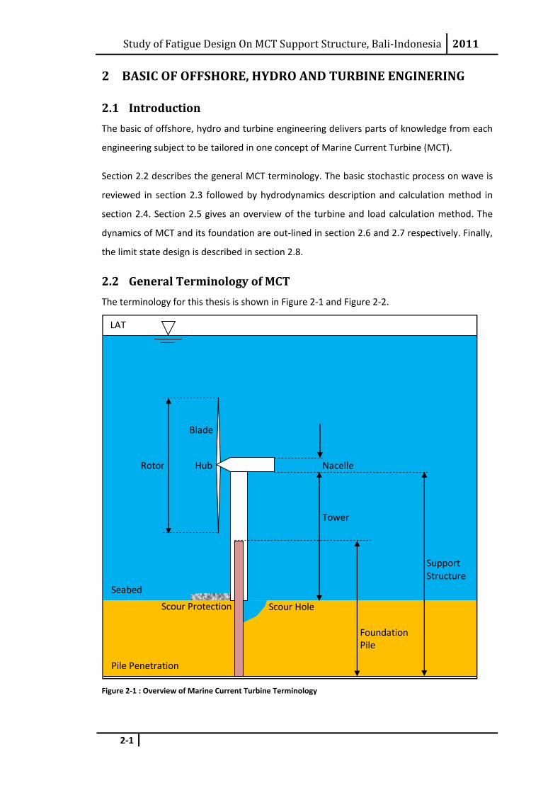
2.2 General Terminology of MCT The terminology for this thesis is shown in Figure 2‐1 and Figure 2‐2.
Figure 2‐1 : Overview of Marine Current Turbine Terminology
Pile Penetration
LAT
Seabed
Scour Protection Scour Hole
Blade
Hub
Tower
Rotor Nacelle
Support Structure
Foundation Pile
Study of Fatigue Design On MCT Support Structure, Bali‐Indonesia 2011
2‐2
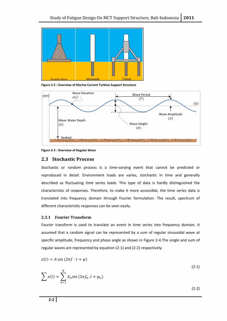
Figure 2‐2 : Overview of Marine Current Turbine Support Structure
Figure 2‐3 : Overview of Regular Wave
2.3 Stochastic Process Stochastic or random process is a time‐varying event that cannot be predicted or
reproduced in detail. Environment loads are varies, stochastic in time and generally
described as fluctuating time series loads. This type of data is hardly distinguished the
characteristic of responses. Therefore, to make it more accessible, the time series data is
translated into frequency domain through Fourier formulation. The result, spectrum of
different characteristic responses can be seen easily.
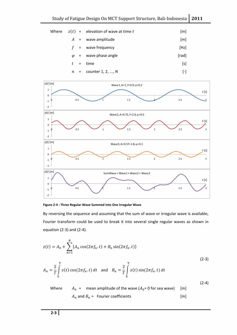
2.3.1 Fourier Transform
Fourier transform is used to translate an event in time series into frequency domain. It
assumed that a random signal can be represented by a sum of regular sinusoidal wave at
specific amplitude, frequency and phase angle as shown in Figure 2‐4.The single and sum of
regular waves are represented by equation (2‐1) and (2‐2) respectively.
sin 2 ·
(2‐1)
sin 2 .
(2‐2)
Gravity Base Monopile Tripod
‐6
‐5
‐4
‐3
‐2
‐1
0
1
2
0 0.5 1 1.5 2 2.5 3
[m]
[s]
Wave Period
Wave Height
Seabed
Mean Water Depth
Wave Elevation
Wave Amplitude
Study of Fatigue Design On MCT Support Structure, Bali‐Indonesia 2011
2‐3
Where = elevation of wave at time t [m]
= wave amplitude [m]
= wave frequency [Hz]
= wave phase angle [rad]
= time [s]
= counter 1, 2, ..., N [‐]
Figure 2‐4 : Three Regular Wave Summed into One Irregular Wave
By reversing the sequence and assuming that the sum of wave or irregular wave is available,
Fourier transform could be used to break it into several single regular waves as shown in
equation (2‐3) and (2‐4).
cos 2 . sin 2 .
(2‐3)
2cos 2 . and
2sin 2 .
(2‐4) Where = mean amplitude of the wave ( = 0 for sea wave) [m]
and = Fourier coefficients [m]
‐2
‐1
0
1
2
0 0.5 1 1.5 2 2.5 3
Wave1, A=1, f=0.9, ϕ=0.2
‐2
‐1
0
1
2
0 0.5 1 1.5 2 2.5 3
Wave2, A=0.75, f=2.0, ϕ=0.5
‐2
‐1
0
1
2
0 0.5 1 1.5 2 2.5 3
Wave3, A=0.5 f=1.8, ϕ=0.1
‐2
‐1
0
1
2
0 0.5 1 1.5 2 2.5 3
SumWave = Wave1 + Wave2 + Wave3z(t) [m]
t [s]
z(t) [m]
t [s]
z(t) [m]
t [s]
z(t) [m]
t [s]
Study of Fatigue Design On MCT Support Structure, Bali‐Indonesia 2011
2‐4
= wave frequency of nth Fourier component [Hz]
T = duration of measurement (T = N ∆t) [s]
∆t = time step [s]
= counter 1, 2, ..., N [‐]
N = total number of time steps [‐]
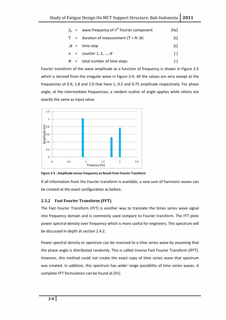
Fourier transform of the wave amplitude as a function of frequency is shown in Figure 2‐5
which is derived from the irregular wave in Figure 2‐4. All the values are zero except at the
frequencies of 0.9, 1.8 and 2.0 that have 1, 0.5 and 0.75 amplitude respectively. For phase
angle, at the intermediate frequencies, a random scatter of angle applies while others are
exactly the same as input value.
Figure 2‐5 : Amplitude versus Frequency as Result from Fourier Transform
If all information from the Fourier transform is available, a new sum of harmonic waves can
be created at the exact configuration as before.
2.3.2 Fast Fourier Transform (FFT)
The Fast Fourier Transform (FFT) is another way to translate the times series wave signal
into frequency domain and is commonly used compare to Fourier transform. The FFT plots
power spectral density over frequency which is more useful for engineers. This spectrum will
be discussed in depth at section 2.4.2.
Power spectral density or spectrum can be reversed to a time series wave by assuming that
the phase angle is distributed randomly. This is called Inverse Fast Fourier Transform (IFFT).
However, this method could not create the exact copy of time series wave that spectrum
was created. In addition, this spectrum has wider range possibility of time series waves. A
complete FFT formulation can be found at [41].
0
0.2
0.4
0.6
0.8
1
1.2
0 0.5 1 1.5 2 2.5
Amplitu
de [m
]
frequncy [Hz]

Study of Fatigue Design On MCT Support Structure, Bali‐Indonesia 2011
2‐5
2.4 Hydrodynamics The motion of the water or hydrodynamics is caused by velocity and acceleration of the
water particles. These components are normally seen as current and wave in the ocean and
acting as loads to the MCT. As the MCT is exposed to both aspects, therefore it will be
discussed in this section.
2.4.1 Current Description
Currents are driven by tides, ocean circulation, river flow, temperature different, salinity and
storm surge. The velocity produced by these sources are varies in space and time. The length
and timescale of the variation in current velocity are much larger compare to the associate
loadings in the design of MCT, therefore, it is assumed that the surface current velocity and
direction to be constant in the design calculations.
In this thesis, the current model for MCT design is defined by a simple current profile over
depth with the power law profile taken from [1] and expressed in equation (2‐5).
0
(2‐5)
Where = current velocity at elevation [m/s]
= current velocity at sea surface ( = 0) [m/s]
= vertical coordinate, positive upward from MSL [m]
= mean water depth [m]
2.4.2 Wave Description
The wave climate at specific location is described as statistical parameters of random
process that remain constant (stationary) for every 3 hours. This characteristic is called
seastate and can be plotted as power density spectra or spectrum in short through FFT.
Two commonly used spectrums are:
• Pierson‐Moskowitz (PM) wave spectrum, for fully developed seas
• JONSWAP wave spectrum, for fetch limited wind generated seas
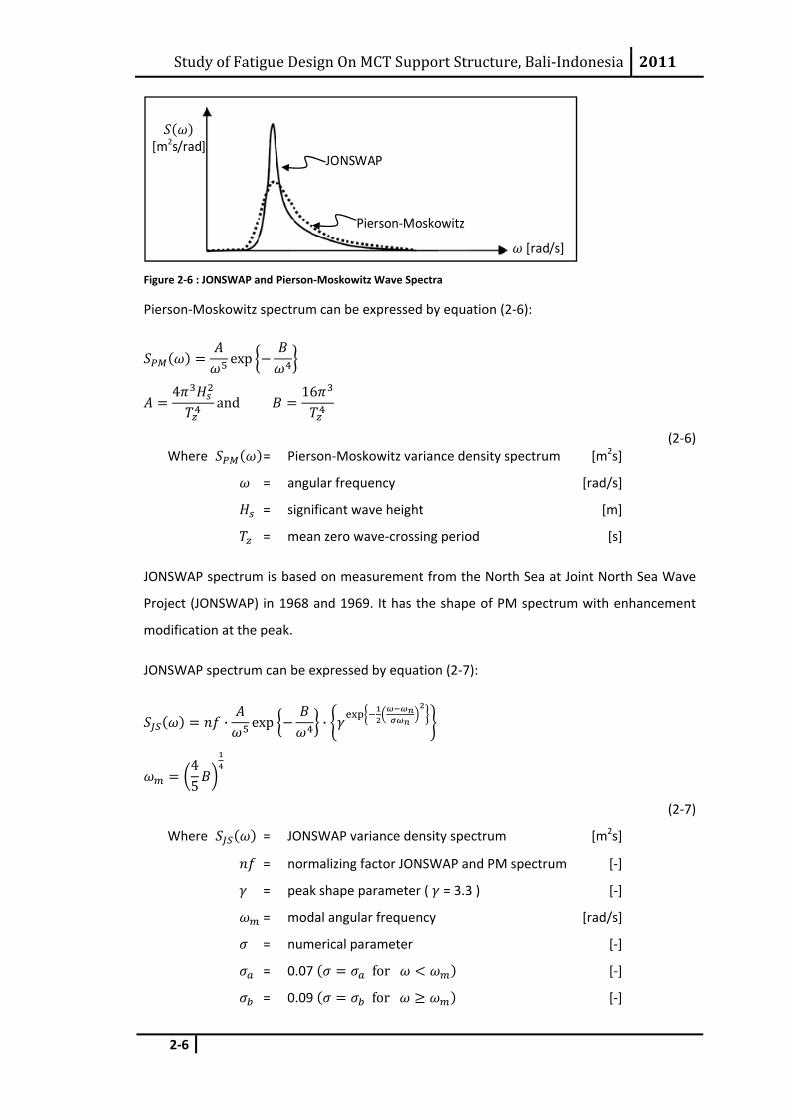
Figure 2‐6 shows the PM and JONSWAP wave spectra. Both spectra are derived from
significant wave height and mean zero‐crossing wave period .
Study of Fatigue Design On MCT Support Structure, Bali‐Indonesia 2011
2‐6
Figure 2‐6 : JONSWAP and Pierson‐Moskowitz Wave Spectra
Pierson‐Moskowitz spectrum can be expressed by equation (2‐6):
exp
4and
16
(2‐6) Where = Pierson‐Moskowitz variance density spectrum [m2s]
= angular frequency [rad/s]
= significant wave height [m]
= mean zero wave‐crossing period [s]
JONSWAP spectrum is based on measurement from the North Sea at Joint North Sea Wave
Project (JONSWAP) in 1968 and 1969. It has the shape of PM spectrum with enhancement
modification at the peak.
JONSWAP spectrum can be expressed by equation (2‐7):
· exp ·
45
(2‐7)
Where = JONSWAP variance density spectrum [m2s]
= normalizing factor JONSWAP and PM spectrum [‐]
= peak shape parameter ( = 3.3 ) [‐]
= modal angular frequency [rad/s]
= numerical parameter [‐]
= 0.07 for [‐]
= 0.09 for [‐]
JONSWAP
Pierson‐Moskowitz
[rad/s]
[m2s/rad]

Study of Fatigue Design On MCT Support Structure, Bali‐Indonesia 2011
2‐7
The average value for , and were taken from measurement of the Joint North Sea
Wave Project. The offshore group at the Delft University of Technology found a normalizing
factor of:
= 0.625 ( for = 3.3 ) [‐]
With the parameters given above, the JONSWAP spectrum can be expressed by and at
equation (2‐8).
2.5 · exp16
· 3.3
12.8 ·
(2‐8)
With the appropriate spectrum, IFFT can be performed to create regular sinusoid waves.
These harmonic waves are translated into velocity and acceleration for load calculation
through linear wave theory of Airy [22]. The horizontal water particle kinematics is
expressed by equation (2‐9).
, · ·cosh
sinh· cos φ
, · ·cosh
sinh· sin φ
(2‐9)
Where , = wave horizontal water particle velocity [m/s]
, = wave horizontal water particle acceleration [m/s2]
= wave amplitude ( = H ) [m]
= wave number ( k = 2π/ ) [rad/m]
= vertical coordinate, positive upward from MSL [m]
= mean water depth [m]
= wave length tanh [m]
= acceleration of gravity [m/s2]
H = wave height [m]
2.4.3 Hydrodynamic Loads on Pile
As mentioned earlier, velocities and accelerations of water particles cause hydrodynamic
loads in the structure. For slender piles, the loading are described by Morison equation as

Study of Fatigue Design On MCT Support Structure, Bali‐Indonesia 2011
2‐8
expressed by equation (2‐10). It named after J.R Morison who derived the formulation in
1950. Morison formulae cover the total hydrodynamic loads from drag and inertia.
4
· 12
· | |
(2‐10)
Where = hydrodynamic load per unit length [N/m]
= hydrodynamic inertia load per unit length [N/m]
= hydrodynamic drag load per unit length [N/m]
= inertia coefficient [‐]
= drag coefficient [‐]
= diameter of pile [m]
= mass density of water [kg/m3]
= horizontal water particle acceleration [m/s2]
= horizontal water particle velocity [m/s]
The Morison equation is based on experiments, therefore the inertia and drag coefficient
are found in many variety. For tubular members, the following drag and inertia wave force
coefficients should be used as per API RP 2A:
= 0.8 for rough members = 0.5 for smooth members = 2.0
The horizontal particle velocity for loading calculation depends on current, wave and the
motion of the structure. Therefore equation (2‐11) accounts the relative aspects of the
velocity acting on structure.
, , ,
(2‐11)
Where , = relative velocity of water to structure [m/s]
= current velocity [m/s]
, = wave horizontal water particle velocity [m/s]
, = structure horizontal velocity [m/s]
The equation (2‐10) can be rewritten due to the total motion in the structure at (2‐12).
4·
41 ·
12
· | |
(2‐12)
Study of Fatigue Design On MCT Support Structure, Bali‐Indonesia 2011
2‐9
2.4.4 Hydrodynamic Loads on Turbine
The hydrodynamic loads on turbine are defined by three theories; momentum, blade
element and blade element momentum theory. Each theory will be discussed in depth at the
following sections.
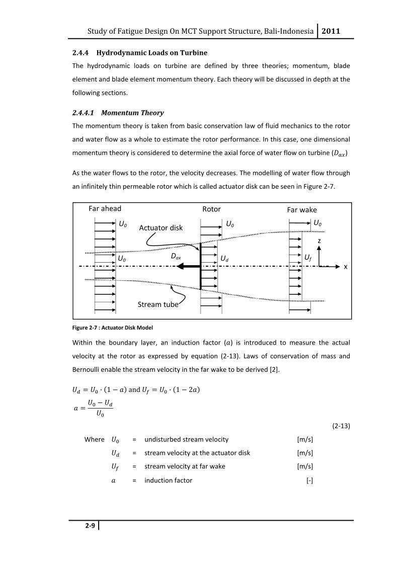
2.4.4.1 Momentum Theory
The momentum theory is taken from basic conservation law of fluid mechanics to the rotor
and water flow as a whole to estimate the rotor performance. In this case, one dimensional
momentum theory is considered to determine the axial force of water flow on turbine ( )
As the water flows to the rotor, the velocity decreases. The modelling of water flow through
an infinitely thin permeable rotor which is called actuator disk can be seen in Figure 2‐7.
Figure 2‐7 : Actuator Disk Model
Within the boundary layer, an induction factor ( ) is introduced to measure the actual
velocity at the rotor as expressed by equation (2‐13). Laws of conservation of mass and
Bernoulli enable the stream velocity in the far wake to be derived [2].
· 1 and · 1 2
(2‐13)
Where = undisturbed stream velocity [m/s]
= stream velocity at the actuator disk [m/s]
= stream velocity at far wake [m/s]
= induction factor [‐]
x
z
Far ahead Rotor Far wake
Actuator disk
Stream tube
U0 U0 U0
U0 Ud Uf Dax
Study of Fatigue Design On MCT Support Structure, Bali‐Indonesia 2011
2‐10
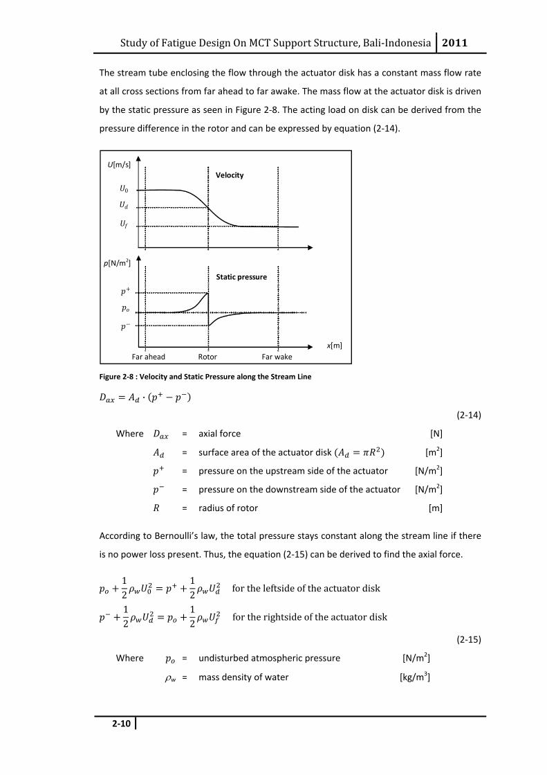
The stream tube enclosing the flow through the actuator disk has a constant mass flow rate
at all cross sections from far ahead to far awake. The mass flow at the actuator disk is driven
by the static pressure as seen in Figure 2‐8. The acting load on disk can be derived from the
pressure difference in the rotor and can be expressed by equation (2‐14).
Figure 2‐8 : Velocity and Static Pressure along the Stream Line
·
(2‐14)
Where = axial force [N]
= surface area of the actuator disk [m2]
= pressure on the upstream side of the actuator [N/m2]
= pressure on the downstream side of the actuator [N/m2]
= radius of rotor [m]
According to Bernoulli’s law, the total pressure stays constant along the stream line if there
is no power loss present. Thus, the equation (2‐15) can be derived to find the axial force.
12
12
for the leftside of the actuator disk
12
12 for the rightside of the actuator disk
(2‐15)
Where = undisturbed atmospheric pressure [N/m2]
ρw = mass density of water [kg/m3]
Far ahead Rotor Far wake
0
U[m/s]
p[N/m2]
x[m]
Static pressure
Velocity

Study of Fatigue Design On MCT Support Structure, Bali‐Indonesia 2011
2‐11
The axial force can be extracted by substituting equation (2‐14) and (2‐15) as shown in
equation (2‐16).
·12· · · 4 1
(2‐16)
The axial force can also be expressed into dimensionless axial force coefficient by equation
(2‐17).
· · · · 4 1
· · ·4 1
(2‐17)
Where = axial force coefficient [‐]
= undisturbed current force [N]
Equation (2‐17) describes the relationship between undisturbed current force, axial
coefficient and the induction factor. However, the induction factor remains unknown. The
blade element theory on section 2.4.4.2 provides the alternative to find the axial force
coefficient which involves the induction factor.
2.4.4.2 Blade Element Theory
The blade element theory assumed that the blade is divided into small elements with
constant cross sections as shown in Figure 2‐9. From the cross section, two‐dimensional
analysis is made with assumptions:
• No hydrodynamic interaction between elements
• The lift and drag forces are the only load acting on the hydrofoil
Figure 2‐9 : Elements of a Blade
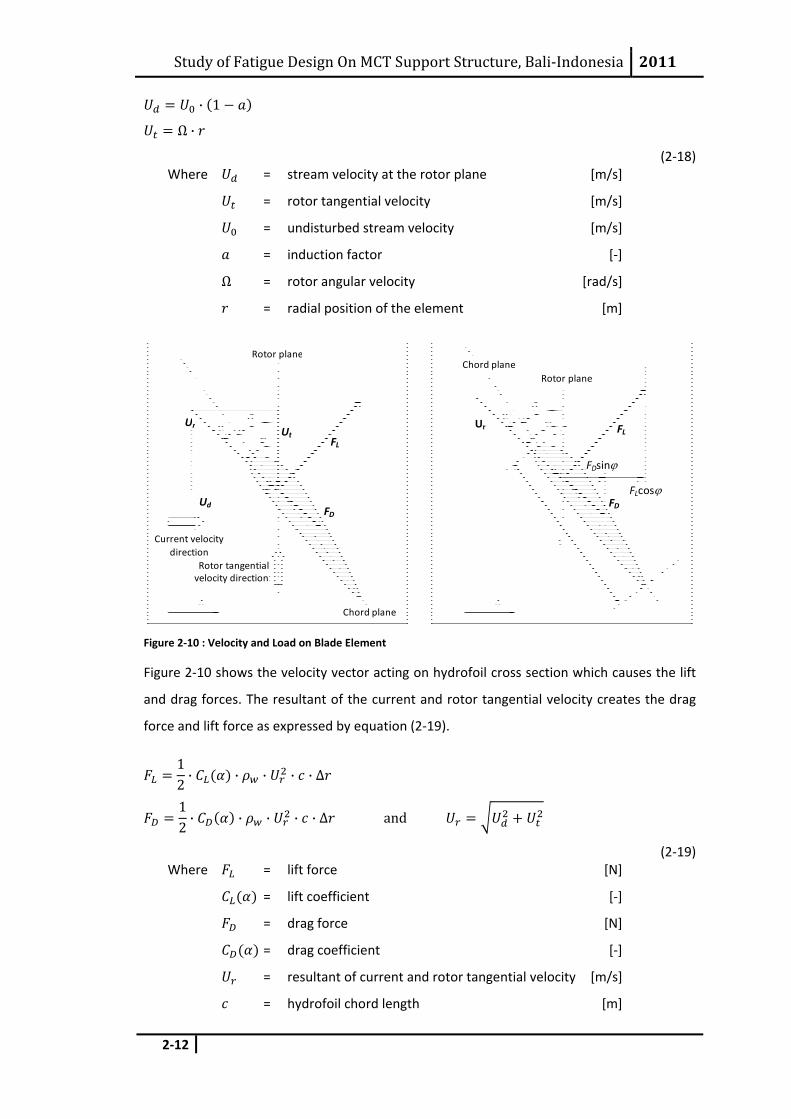
The lift and drag forces are caused by stream velocity at the rotor and the rotor tangential
velocity as expressed in equation (2‐18) and illustrated by Figure 2‐10.
Study of Fatigue Design On MCT Support Structure, Bali‐Indonesia 2011
2‐12
· 1
Ω ·
(2‐18) Where = stream velocity at the rotor plane [m/s]
= rotor tangential velocity [m/s]
= undisturbed stream velocity [m/s]
= induction factor [‐]
Ω = rotor angular velocity [rad/s]
= radial position of the element [m]
Figure 2‐10 : Velocity and Load on Blade Element
Figure 2‐10 shows the velocity vector acting on hydrofoil cross section which causes the lift
and drag forces. The resultant of the current and rotor tangential velocity creates the drag
force and lift force as expressed by equation (2‐19).
12· · · · · Δ
12· · · · · Δ and
(2‐19) Where = lift force [N]
= lift coefficient [‐]
= drag force [N]
= drag coefficient [‐]
= resultant of current and rotor tangential velocity [m/s]
= hydrofoil chord length [m]
Ur
Ud
Ut
Current velocity direction
Rotor tangential velocity direction
Rotor plane
Chord plane
FD
FL
Ur
Chord plane Rotor plane
FL
FD
FDsinϕ
FLcosϕ
Study of Fatigue Design On MCT Support Structure, Bali‐Indonesia 2011
2‐13
Δ = radial length of blade element [m]
= angle of attack [deg]
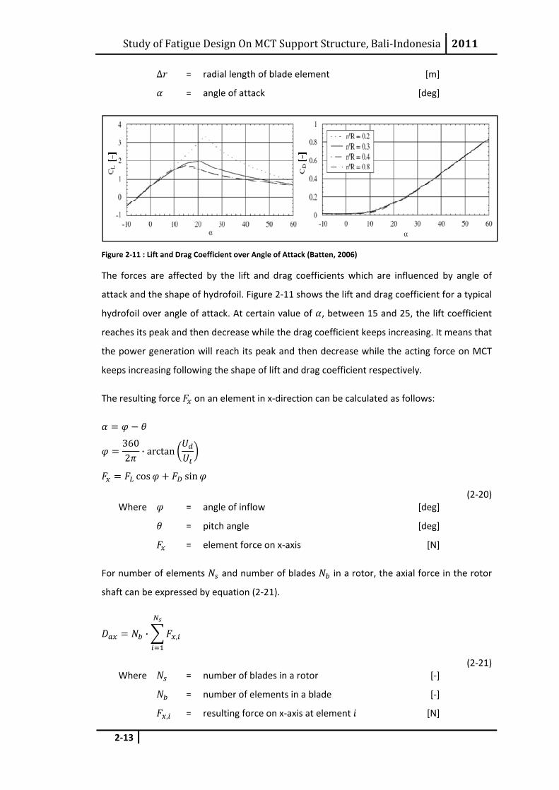
Figure 2‐11 : Lift and Drag Coefficient over Angle of Attack (Batten, 2006)
The forces are affected by the lift and drag coefficients which are influenced by angle of
attack and the shape of hydrofoil. Figure 2‐11 shows the lift and drag coefficient for a typical
hydrofoil over angle of attack. At certain value of , between 15 and 25, the lift coefficient
reaches its peak and then decrease while the drag coefficient keeps increasing. It means that
the power generation will reach its peak and then decrease while the acting force on MCT
keeps increasing following the shape of lift and drag coefficient respectively.
The resulting force on an element in x‐direction can be calculated as follows:
3602
· arctan
cos sin
(2‐20) Where = angle of inflow [deg]
= pitch angle [deg]
= element force on x‐axis [N]
For number of elements and number of blades in a rotor, the axial force in the rotor
shaft can be expressed by equation (2‐21).
· ,
(2‐21) Where = number of blades in a rotor [‐]
= number of elements in a blade [‐]
, = resulting force on x‐axis at element [N]
Study of Fatigue Design On MCT Support Structure, Bali‐Indonesia 2011
2‐14
The axial force coefficient using blade element theory now can be derived by equation
(2‐22).
· ∑ ,
· · ·
(2‐22) Where = axial force coefficient [‐]
= undisturbed current force [N]
To be note that the axial coefficient depends on induction factor as it was used in equation
(2‐17) and remains unknown. In the next section, both momentum and blade element
theories will be combined to determine the induction factor as well as the axial force.
2.4.4.3 Blade Element Momentum Theory
The blade element momentum (BEM) theory combines the momentum theory and the
blade element theory to determine the axial force acting on turbine. According to BEM
theory, the axial coefficients from momentum and blade element theories are equal as
expressed in equation (2‐23). Both coefficients are induction factor dependent which now
can be calculated. It appears at range of 0 and 0.5 for no current velocity decrease at
actuator disk and velocity in far wake becomes zero respectively.
, ,
(2‐23) Where , = axial force coefficient from momentum theory [‐]
, = axial force coefficient from blade element theory [‐]
Once the induction factor has been found, the hydrodynamic axial force on turbine can be
determined by equation (2‐24).
· · ·12· ·
(2‐24)
2.5 Turbine Description Many arrangements arrived in the marine current energy converter such as horizontal axis
turbine, vertical axis turbine, hydrofoil device and venturi devices. The horizontal axis
turbine has been developed in advance on wind energy converter, which gives more
advantages compare to other devices. With the same mechanism of wind energy extraction,
the horizontal axis turbine presently is being desired in current energy development and
therefore will be used and discussed further in this thesis.
Study of Fatigue Design On MCT Support Structure, Bali‐Indonesia 2011
2‐15
Unlike the wind turbine that has its own market and brand, the horizontal axis MCT
currently is at a prototype stage, where single devices are placed at isolated testing site.
Therefore the MCT selection will be based on assumption and developed from wind turbine
as well as MCT most recent research.
2.5.1 Power Capture
Power capture of MCT is the main topic for tidal power generation. As the current stream
flows through the blades and drives the blades into a certain tip speed, thus, power is
generated. The maximum power generation is created at a certain blade rotational speed
which influences the fatigue design.
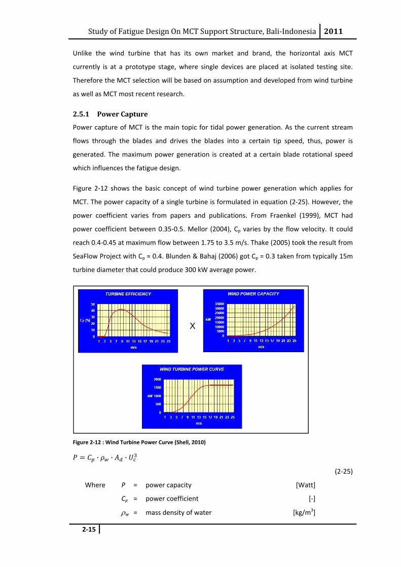
Figure 2‐12 shows the basic concept of wind turbine power generation which applies for
MCT. The power capacity of a single turbine is formulated in equation (2‐25). However, the
power coefficient varies from papers and publications. From Fraenkel (1999), MCT had
power coefficient between 0.35‐0.5. Mellor (2004), Cp varies by the flow velocity. It could
reach 0.4‐0.45 at maximum flow between 1.75 to 3.5 m/s. Thake (2005) took the result from
SeaFlow Project with Cp ≈ 0.4. Blunden & Bahaj (2006) got Cp = 0.3 taken from typically 15m
turbine diameter that could produce 300 kW average power.
Figure 2‐12 : Wind Turbine Power Curve (Shell, 2010)
· · ·
(2‐25)
Where P = power capacity [Watt]
Cp = power coefficient [‐]
ρw = mass density of water [kg/m3]
Study of Fatigue Design On MCT Support Structure, Bali‐Indonesia 2011
2‐16
Ad = surface area of actuator disc [m2]
= current velocity [m/s]
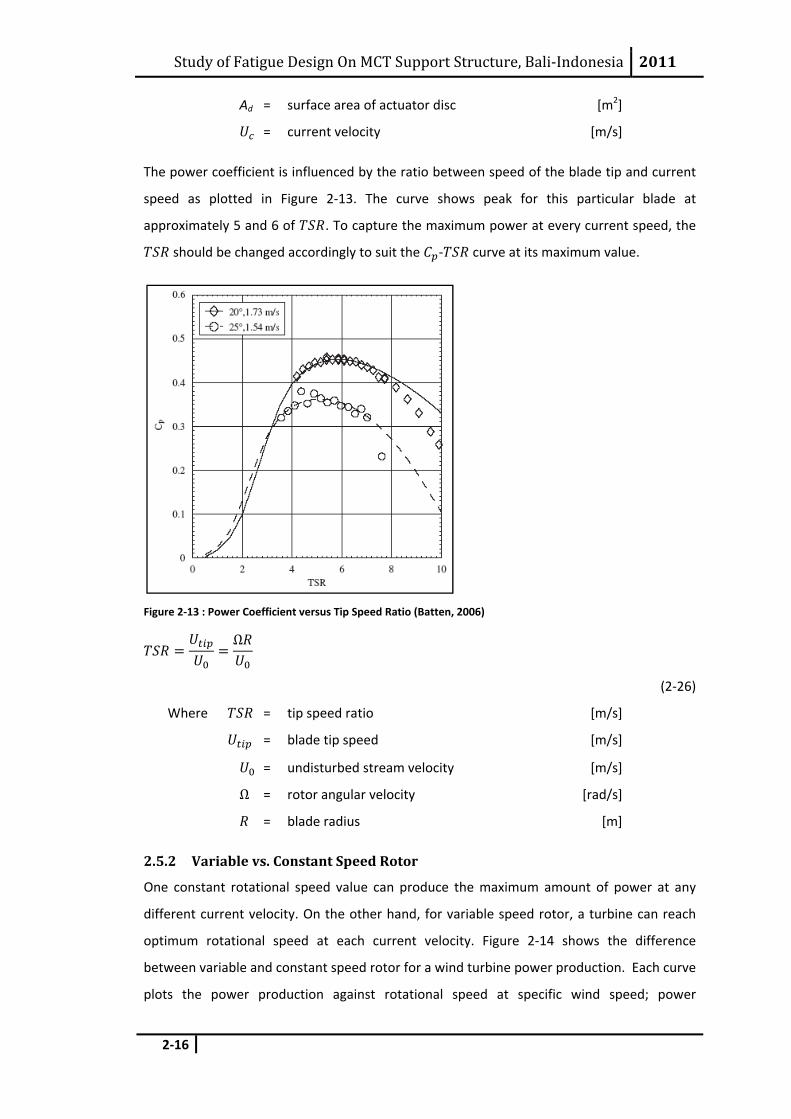
The power coefficient is influenced by the ratio between speed of the blade tip and current
speed as plotted in Figure 2‐13. The curve shows peak for this particular blade at
approximately 5 and 6 of . To capture the maximum power at every current speed, the
should be changed accordingly to suit the ‐ curve at its maximum value.
Figure 2‐13 : Power Coefficient versus Tip Speed Ratio (Batten, 2006)
Ω
(2‐26)
Where = tip speed ratio [m/s]
= blade tip speed [m/s]
= undisturbed stream velocity [m/s]
Ω = rotor angular velocity [rad/s]
= blade radius [m]
2.5.2 Variable vs. Constant Speed Rotor
One constant rotational speed value can produce the maximum amount of power at any
different current velocity. On the other hand, for variable speed rotor, a turbine can reach
optimum rotational speed at each current velocity. Figure 2‐14 shows the difference
between variable and constant speed rotor for a wind turbine power production. Each curve
plots the power production against rotational speed at specific wind speed; power
Study of Fatigue Design On MCT Support Structure, Bali‐Indonesia 2011
2‐17
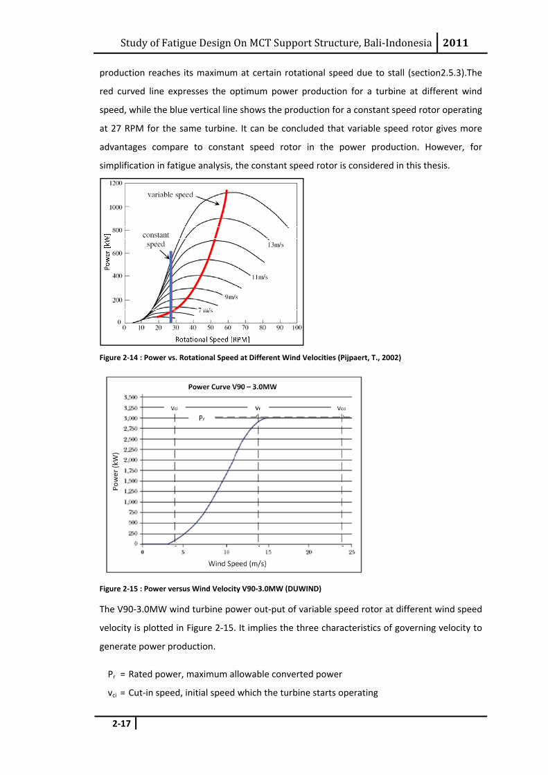
production reaches its maximum at certain rotational speed due to stall (section2.5.3).The
red curved line expresses the optimum power production for a turbine at different wind
speed, while the blue vertical line shows the production for a constant speed rotor operating
at 27 RPM for the same turbine. It can be concluded that variable speed rotor gives more
advantages compare to constant speed rotor in the power production. However, for
simplification in fatigue analysis, the constant speed rotor is considered in this thesis.
Figure 2‐14 : Power vs. Rotational Speed at Different Wind Velocities (Pijpaert, T., 2002)
Figure 2‐15 : Power versus Wind Velocity V90‐3.0MW (DUWIND)
The V90‐3.0MW wind turbine power out‐put of variable speed rotor at different wind speed
velocity is plotted in Figure 2‐15. It implies the three characteristics of governing velocity to
generate power production.
Pr = Rated power, maximum allowable converted power
vci = Cut‐in speed, initial speed which the turbine starts operating
Study of Fatigue Design On MCT Support Structure, Bali‐Indonesia 2011
2‐18
vr = Rated/nominal speed, the lowest speed which Pr is reached
vco = Cut‐out speed, the maximum speed which operations are stopped.
The speed characteristic defines four different intervals for turbine operation. Below cut‐in
speed, no power will be generated due to mechanical friction is higher than incoming
energy. Between cut‐in and rated speed, maximum power is generated according to the
occurring speed. At the rated speed, the generator reaches the maximum power to be
converted. Above this speed, there will be an excessive power production which could
damage the generator. As the ideal condition is to keep the power at constant value of Pr,
therefore, stall of pitch regulation is applied as power control. At last, above the cut‐out
speed, no power will be generated in order to prevent extreme loading.
2.5.3 Stall vs. Pitch Regulated Power Control
Two techniques have been developed in order to control turbine power generation once the
occurring speed exceeded the rated speed. Stall regulated power control mostly can be
found in constant speed rotor, while variable speed rotor are commonly used pitch
regulated.
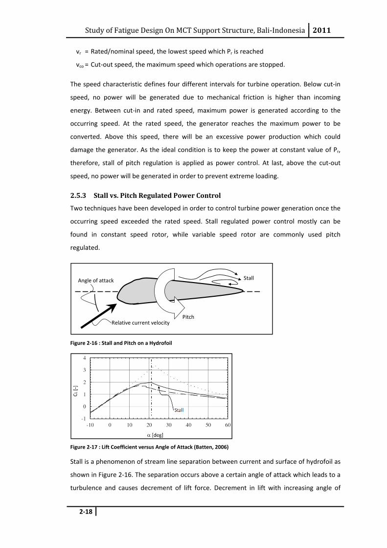
Figure 2‐16 : Stall and Pitch on a Hydrofoil
Figure 2‐17 : Lift Coefficient versus Angle of Attack (Batten, 2006)
Stall is a phenomenon of stream line separation between current and surface of hydrofoil as
shown in Figure 2‐16. The separation occurs above a certain angle of attack which leads to a
turbulence and causes decrement of lift force. Decrement in lift with increasing angle of
Pitch
Angle of attack
Relative current velocity
Stall
Study of Fatigue Design On MCT Support Structure, Bali‐Indonesia 2011
2‐19
attack can be set as definition of stall (Corten, 2001) as shown in Figure 2‐17. When current
velocity increases at a constant rotor speed, the angle of attack will increase; and at a
certain current velocity, the blades will begin to stall. This will cause decrement in lift but on
the other hand the drag will keep on increasing. At this point, there will be no power
increment even with higher current velocity. The stall regulated system is the simplest
technique, since it fixed to the hub and cannot be pitched.
Pitch regulated power control enables the blades rotating at its longitudinal axis therefore
the angle of attack can be changed simultaneously. Increment in pitch decreases angle of
attack and decrement angle of attack reduces lift coefficient as shown Figure 2‐16 and
Figure 2‐17 respectively. This phenomenon will decrease the power generation as well. Thus,
when the rated power is achieved and the current speed rises above the rated speed, the
power can be kept constant at rated power value through a pitch adjustment. It is also
possible to reduce power generation by pitching the blades at opposite direction which
increases the angle of attack. This technique is called active stall regulated power control.
2.6 Dynamics of Marine Current Turbine The MCT is exposed to the dynamically changing loads. This section will describe the basic of
equation of motion followed by harmonic excitation from turbine and wave as well as the
hydrodynamic damping as the effect of rotating blades.
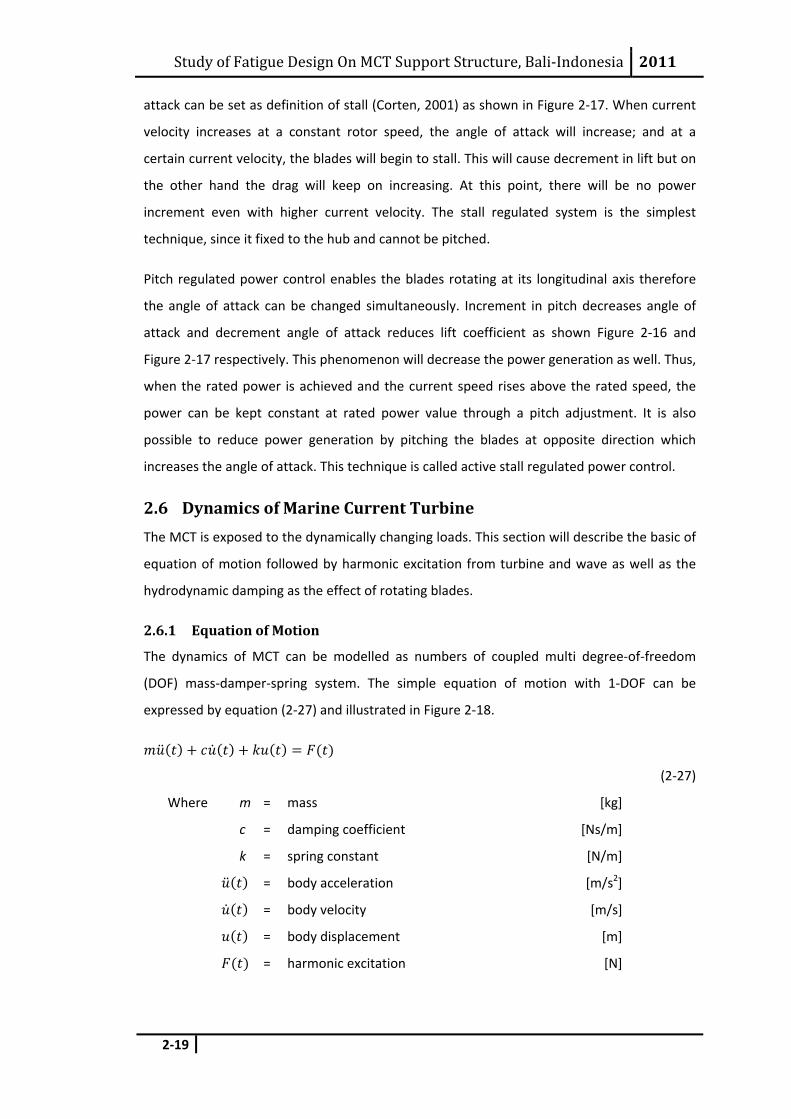
2.6.1 Equation of Motion
The dynamics of MCT can be modelled as numbers of coupled multi degree‐of‐freedom
(DOF) mass‐damper‐spring system. The simple equation of motion with 1‐DOF can be
expressed by equation (2‐27) and illustrated in Figure 2‐18.
(2‐27)
Where m = mass [kg]
c = damping coefficient [Ns/m]
k = spring constant [N/m]
= body acceleration [m/s2]
= body velocity [m/s]
= body displacement [m]
= harmonic excitation [N]
Study of Fatigue Design On MCT Support Structure, Bali‐Indonesia 2011
2‐20
Figure 2‐18 : 1‐DOF mass‐damper‐spring system
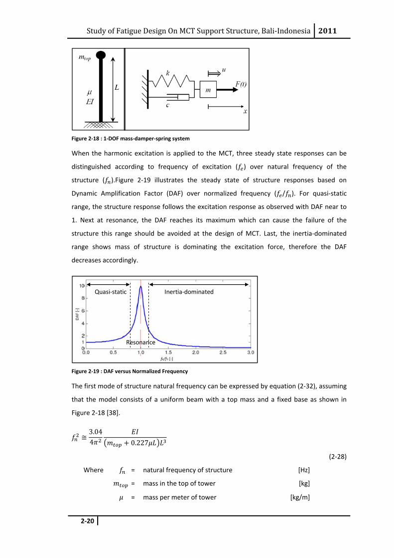
When the harmonic excitation is applied to the MCT, three steady state responses can be
distinguished according to frequency of excitation ( ) over natural frequency of the
structure ( ).Figure 2‐19 illustrates the steady state of structure responses based on
Dynamic Amplification Factor (DAF) over normalized frequency ( / ). For quasi‐static
range, the structure response follows the excitation response as observed with DAF near to
1. Next at resonance, the DAF reaches its maximum which can cause the failure of the
structure this range should be avoided at the design of MCT. Last, the inertia‐dominated
range shows mass of structure is dominating the excitation force, therefore the DAF
decreases accordingly.
Figure 2‐19 : DAF versus Normalized Frequency
The first mode of structure natural frequency can be expressed by equation (2‐32), assuming
that the model consists of a uniform beam with a top mass and a fixed base as shown in
Figure 2‐18 [38].
3.044 0.227
(2‐28)
Where = natural frequency of structure [Hz]
= mass in the top of tower [kg]
= mass per meter of tower [kg/m]
Quasi‐static
Resonance
Inertia‐dominated
Study of Fatigue Design On MCT Support Structure, Bali‐Indonesia 2011
2‐21
= height of tower [m]
= bending stiffness of tower [Nm2]
By using parameters in (2‐29), equation (2‐28) can be re‐written as follows,
18
, and
(2‐29)
104 0.227
(2‐30)
Where = wall thickness of tower [m]
= average diameter of tower (=D ‐ tw) [m]
= density of steel (=7850) [kg/m3]
= young’s modulus (=2.108) [kN/m2]
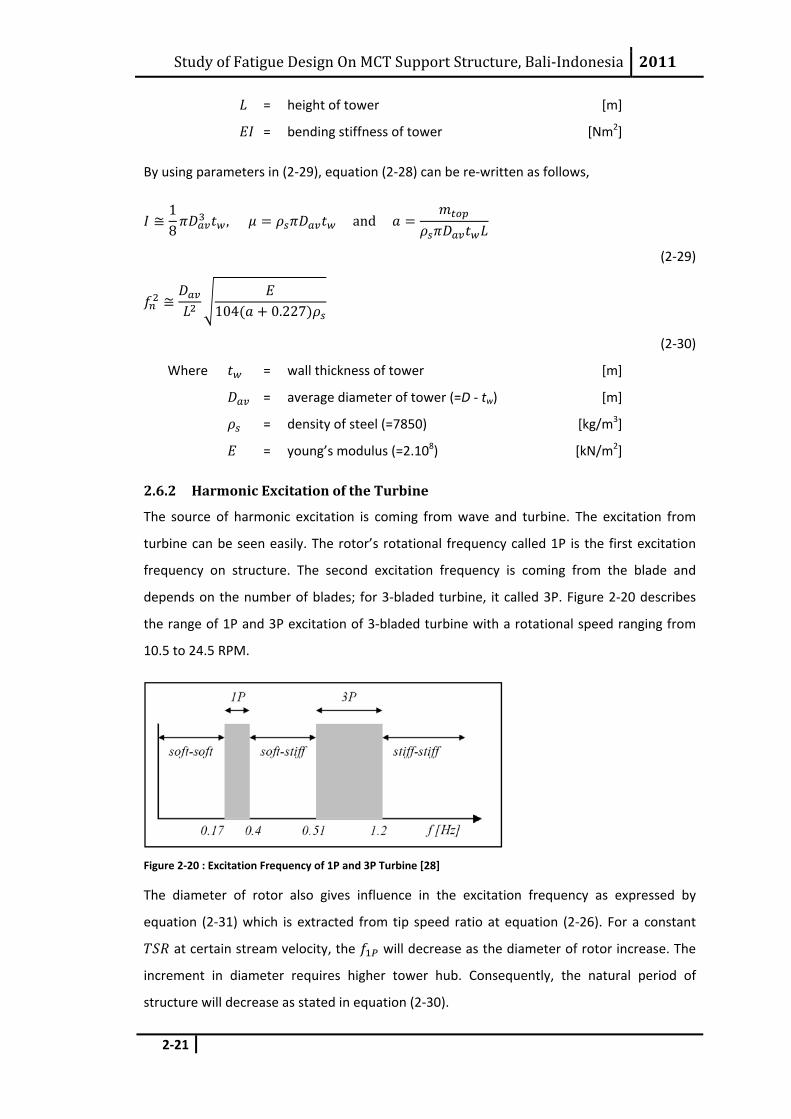
2.6.2 Harmonic Excitation of the Turbine
The source of harmonic excitation is coming from wave and turbine. The excitation from
turbine can be seen easily. The rotor’s rotational frequency called 1P is the first excitation
frequency on structure. The second excitation frequency is coming from the blade and
depends on the number of blades; for 3‐bladed turbine, it called 3P. Figure 2‐20 describes
the range of 1P and 3P excitation of 3‐bladed turbine with a rotational speed ranging from
10.5 to 24.5 RPM.
Figure 2‐20 : Excitation Frequency of 1P and 3P Turbine [28]
The diameter of rotor also gives influence in the excitation frequency as expressed by
equation (2‐31) which is extracted from tip speed ratio at equation (2‐26). For a constant
at certain stream velocity, the will decrease as the diameter of rotor increase. The
increment in diameter requires higher tower hub. Consequently, the natural period of
structure will decrease as stated in equation (2‐30).
Study of Fatigue Design On MCT Support Structure, Bali‐Indonesia 2011
2‐22
as, Ω 2 thus,·
(2‐31) Where = rotor’s rotational frequency [Hz]
= diameter of rotor [m]
It is important to keep the natural frequency of structure outside the range of the turbine’s
frequency bands in order to avoid resonance which causes failure of the structure. Figure
2‐20 defines the outside ranges of turbine harmonic excitation and are categorized as
follows:
• Soft‐soft : structure natural frequency below rotor’s rotational frequency
• Soft‐stiff : structure natural frequency between the rotor's rotational frequency and
blade passing frequency
• Stiff‐stiff : structure natural frequency above the blade passing frequency
The soft‐soft band is more attractive compare to other bands because it requires less
material and thus economically suitable. However, the structural response to fatigue failure
is more sensitive as the wave bands normally appear at low frequency.
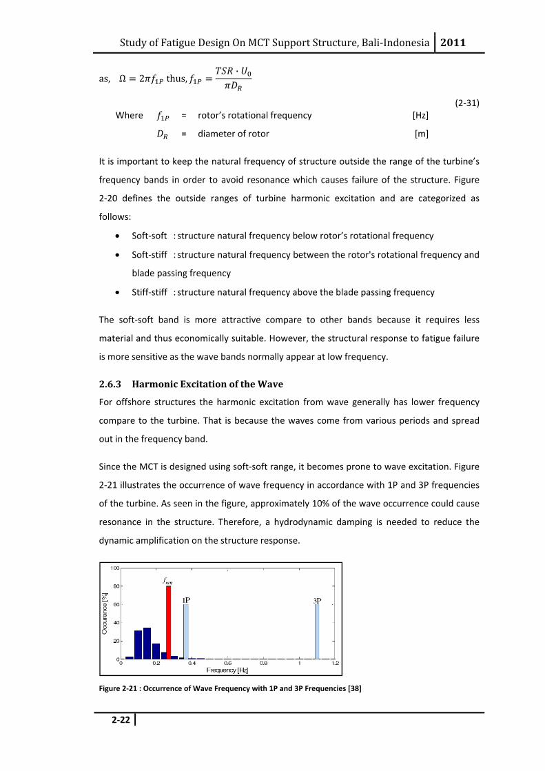
2.6.3 Harmonic Excitation of the Wave
For offshore structures the harmonic excitation from wave generally has lower frequency
compare to the turbine. That is because the waves come from various periods and spread
out in the frequency band.
Since the MCT is designed using soft‐soft range, it becomes prone to wave excitation. Figure
2‐21 illustrates the occurrence of wave frequency in accordance with 1P and 3P frequencies
of the turbine. As seen in the figure, approximately 10% of the wave occurrence could cause
resonance in the structure. Therefore, a hydrodynamic damping is needed to reduce the
dynamic amplification on the structure response.
Figure 2‐21 : Occurrence of Wave Frequency with 1P and 3P Frequencies [38]
Study of Fatigue Design On MCT Support Structure, Bali‐Indonesia 2011
2‐23
2.6.4 Hydrodynamic Damping
When an operating turbine moves against the stream, the blades experience an increasing
load as a result of an increasing stream velocity. This load is acting against the tower top
motion. Analogous for backward movement, it reduces the loading as well as the motion in
the top of tower. This condition is known as hydrodynamic damping.
The hydrodynamic damping due to rotor is modelled into two conditions, low damping of
1.5% in case the turbine is not operating and high damping (5%) for turbine in operation.
This estimation is taken from offshore wind turbine energy [28].
Based on API RP2A, for typical pile founded tubular space frame substructures, a total
damping value of 2% of critical is appropriate. This accounts for all sources of damping
including structural, foundation and hydrodynamic effects.
As an engineering judgement, 4% of hydrodynamic damping at operational condition and 2%
for non‐operating turbine will be considered in this thesis.
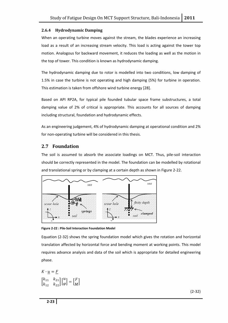
2.7 Foundation The soil is assumed to absorb the associate loadings on MCT. Thus, pile‐soil interaction
should be correctly represented in the model. The foundation can be modelled by rotational
and translational spring or by clamping at a certain depth as shown in Figure 2‐22.
Figure 2‐22 : Pile‐Soil Interaction Foundation Model
Equation (2‐32) shows the spring foundation model which gives the rotation and horizontal
translation affected by horizontal force and bending moment at working points. This model
requires advance analysis and data of the soil which is appropriate for detailed engineering
phase.
·
(2‐32)
Study of Fatigue Design On MCT Support Structure, Bali‐Indonesia 2011
2‐24
Where = stiffness matrix [‐]
= displacement vector [‐]
= load vector [‐]
= spring constant [‐]
= horizontal displacement [m]
= rotation [rad]
= horizontal load [N]
= bending moment [Nm]
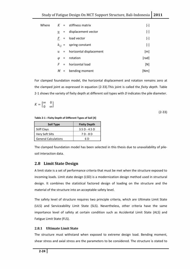
For clamped foundation model, the horizontal displacement and rotation remains zero at
the clamped joint as expressed in equation (2‐33).This joint is called the fixity depth. Table
2‐1 shows the variety of fixity depth at different soil types with D indicates the pile diameter.
∞ 00 ∞
(2‐33)
Table 2‐1 : Fixity Depth of Different Types of Soil [4]
Soil Type Fixity Depth
Stiff Clays 3.5 D ‐ 4.5 D
Very Soft Silts 7 D ‐ 8 D
General Calculations 6 D
The clamped foundation model has been selected in this thesis due to unavailability of pile‐
soil interaction data.
2.8 Limit State Design A limit state is a set of performance criteria that must be met when the structure exposed to
incoming loads. Limit state design (LSD) is a modernization design method used in structural
design. It combines the statistical factored design of loading on the structure and the
material of the structure into an acceptable safety level.
The safety level of structure requires two principle criteria, which are Ultimate Limit State
(ULS) and Serviceability Limit State (SLS). Nevertheless, other criteria have the same
importance level of safety at certain condition such as Accidental Limit State (ALS) and
Fatigue Limit State (FLS).
2.8.1 Ultimate Limit State
The structure must withstand when exposed to extreme design load. Bending moment,
shear stress and axial stress are the parameters to be considered. The structure is stated to

Study of Fatigue Design On MCT Support Structure, Bali‐Indonesia 2011
2‐25
be safe when the factored magnified loadings are less than the factored reduced resistance
of the material.
2.8.2 Service Limit State
The structure must remain functioned as intended when subjected to daily routine loadings.
The main purpose of SLS is to ensure that personnel in the structure are not unnerved by
large deflection on the floor. Since the MCT is designed to be unmanned, therefore the SLS
design is set as required.
2.8.3 Accidental Limit State
The structure must withstand when exposed to excessive structural damage as
consequences of accident which affects the integrity of the structure, environment and
personnel. The ALS could be, for example, collision of maintenance boat with the MCT,
explosion of MCT due to excessive power production or electrical leak on generator and/or
ground acceleration which causes seismic and tsunami.
2.8.4 Fatigue Limit State
The structure must withstand when exposed to cyclic loading that causes fatigue crack due
to stress concentration and damage accumulation. This thesis will discuss in depth the
fatigue design of MCT due to cyclic loading of wave and turbine at chapter 3.

Study of Fatigue Design On MCT Support Structure, Bali‐Indonesia 2011
3‐1
3 FATIGUE DESIGN TERMINOLOGY
3.1 Introduction
Fatigue is a process of progressive localized permanent structural change in a material
subjected to fluctuating stresses and strains at particular points that lead into cracks or
complete fracture after a sufficient numbers of fluctuations. Marine current turbine (MCT) is
exposed to fluctuating loads from wave and turbine. Therefore, the stress responses are
varies in time which making MCT is prone to fatigue damage.
This chapter will expose the fatigue terminology starting with comparing the time series and
frequency domain at section 3.2 and the principles of fatigue analysis afterwards. The
selected fatigue spectral analysis is described in section 3.4 followed by stress concentration
factor in section 3.5. Finally, section 3.6 will discuss the fatigue endurance of MCT support
structure.
3.2 Time Domain vs. Frequency Domain The time domain and frequency domain calculation methods offer two different analysis
techniques for the same system. The main difference is that the time domain represents a
specific of stochastic process and frequency domain covers all stochastically possible
realisations.
The load calculation in frequency domain introduces a non‐linearity through the drag term in
the Morison equation. For offshore structures with pile configurations, it shows that the
linear inertia term is more dominant compare to drag term. This applies for both maximum
waves and smaller waves which induce fatigue loading at reference sites. As this system can
be approached by linear term, the linear frequency domain can assess the fatigue damage
calculation in an effective manner without losing accuracy as compared to time domain
calculations. On the other hand, the time domain offers the exact value which fit in the
excitation loading. It has precision loading as translated from environment condition present
at reference site. However, in the oil and gas industry, this method is barely used due time
consuming in the process of calculation. Therefore, the frequency domain fatigue analysis
will be used and discussed in this thesis.
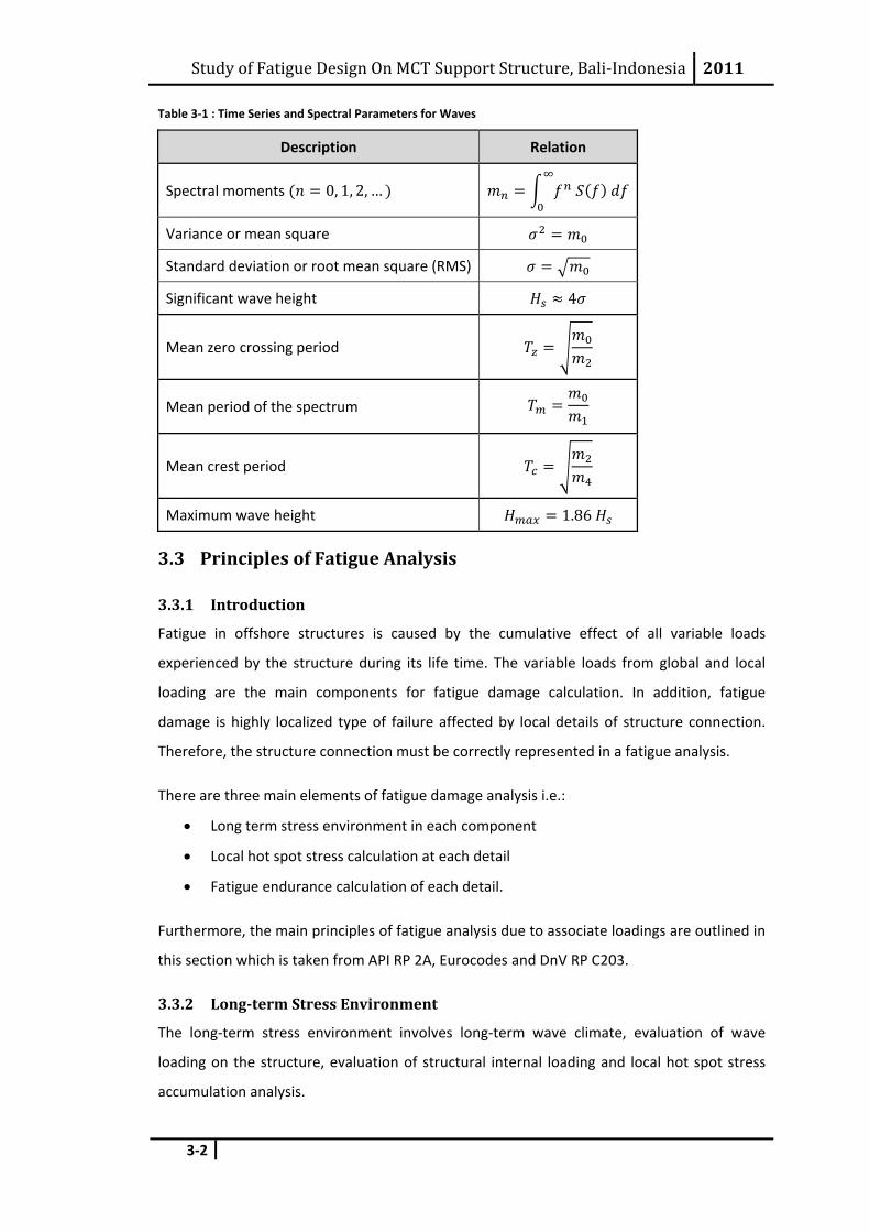
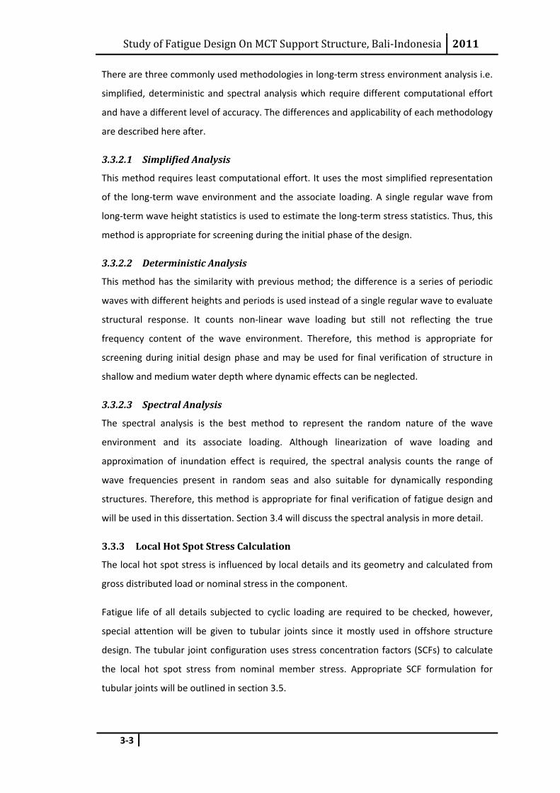
Table 3‐1 provides the relation between time series and spectral parameters for waves
which will be used in this thesis. The spectra formulation of JONSWAP and Pierson‐
Moskowitz can be found at section 2.4.2.
Study of Fatigue Design On MCT Support Structure, Bali‐Indonesia 2011
3‐2
Table 3‐1 : Time Series and Spectral Parameters for Waves
Description Relation
Spectral moments 0, 1, 2, …
Variance or mean square
Standard deviation or root mean square (RMS)
Significant wave height 4
Mean zero crossing period
Mean period of the spectrum
Mean crest period
Maximum wave height 1.86
3.3 Principles of Fatigue Analysis
3.3.1 Introduction
Fatigue in offshore structures is caused by the cumulative effect of all variable loads
experienced by the structure during its life time. The variable loads from global and local
loading are the main components for fatigue damage calculation. In addition, fatigue
damage is highly localized type of failure affected by local details of structure connection.
Therefore, the structure connection must be correctly represented in a fatigue analysis.
There are three main elements of fatigue damage analysis i.e.:
• Long term stress environment in each component
• Local hot spot stress calculation at each detail
• Fatigue endurance calculation of each detail.
Furthermore, the main principles of fatigue analysis due to associate loadings are outlined in
this section which is taken from API RP 2A, Eurocodes and DnV RP C203.
3.3.2 Longterm Stress Environment
The long‐term stress environment involves long‐term wave climate, evaluation of wave
loading on the structure, evaluation of structural internal loading and local hot spot stress
accumulation analysis.
Study of Fatigue Design On MCT Support Structure, Bali‐Indonesia 2011
3‐3
There are three commonly used methodologies in long‐term stress environment analysis i.e.
simplified, deterministic and spectral analysis which require different computational effort
and have a different level of accuracy. The differences and applicability of each methodology
are described here after.
3.3.2.1 Simplified Analysis
This method requires least computational effort. It uses the most simplified representation
of the long‐term wave environment and the associate loading. A single regular wave from
long‐term wave height statistics is used to estimate the long‐term stress statistics. Thus, this
method is appropriate for screening during the initial phase of the design.
3.3.2.2 Deterministic Analysis
This method has the similarity with previous method; the difference is a series of periodic
waves with different heights and periods is used instead of a single regular wave to evaluate
structural response. It counts non‐linear wave loading but still not reflecting the true
frequency content of the wave environment. Therefore, this method is appropriate for
screening during initial design phase and may be used for final verification of structure in
shallow and medium water depth where dynamic effects can be neglected.
3.3.2.3 Spectral Analysis
The spectral analysis is the best method to represent the random nature of the wave
environment and its associate loading. Although linearization of wave loading and
approximation of inundation effect is required, the spectral analysis counts the range of
wave frequencies present in random seas and also suitable for dynamically responding
structures. Therefore, this method is appropriate for final verification of fatigue design and
will be used in this dissertation. Section 3.4 will discuss the spectral analysis in more detail.
3.3.3 Local Hot Spot Stress Calculation
The local hot spot stress is influenced by local details and its geometry and calculated from
gross distributed load or nominal stress in the component.
Fatigue life of all details subjected to cyclic loading are required to be checked, however,
special attention will be given to tubular joints since it mostly used in offshore structure
design. The tubular joint configuration uses stress concentration factors (SCFs) to calculate
the local hot spot stress from nominal member stress. Appropriate SCF formulation for
tubular joints will be outlined in section 3.5.
Study of Fatigue Design On MCT Support Structure, Bali‐Indonesia 2011
3‐4
3.3.4 Fatigue Endurance
The crack growth behaviour under cyclic loading for a particular material and detail defines
the fatigue life of the structure. The fatigue endurance is translated from a given stress
ranges to a number of cycles at particular location through S‐N curve. Both stress range and
number of cycles are in conjunction with long‐term statistics of hot spot stresses and
Miner’s rule. The fatigue endurance which involves S‐N curve and Miner’s rule will be
discussed in section 3.6.
3.3.5 Safety Philosophy
The main objective of fatigue analysis is to verify that the structure is safe due to associate
fatigue loadings during its service life. The safety philosophy of fatigue design is to minimize
the requirement of inspection and additional consideration should be given for inaccessible
or difficult to inspect in‐service area.
The following criteria may be applied for fatigue safety philosophy design:
• Easily accessible inspection should have a minimum calculated design fatigue life of
twice of the intended service life.
• Inaccessible or difficult inspection should have a minimum calculated design fatigue
life of four times the intended service life.
For the MCT support structure design, the details are considered as inaccessible or difficult
to inspect therefore a minimum calculated design fatigue life of four times the intended
service life is required.
3.3.6 Dynamic Analysis
Dynamic analysis is required if the natural periods of the structure are in the range of
associate loadings which could lead to significant dynamic response.
For normal structure configuration in the oil and gas industry, dynamic response to wave can
be ignored if the platform fundamental natural period is less than 3 seconds. And for mono‐
column type of structure, a lower wave period cut‐off should be considered due to no wave
cancelation effect at higher frequency.
3.4 Spectral Fatigue Analysis
3.4.1 Introduction
The spectral fatigue analysis is the most comprehensive analysis and the best way to
represent the random nature of the wave environment. This method uses long‐term
Study of Fatigue Design On MCT Support Structure, Bali‐Indonesia 2011
3‐5
statistics of the wave tabulated in wave scatter diagram to represent the range of wave
frequencies of reference site. These frequencies are explicitly accounted in the loading and
structure response as well as the effect of hot spot stress transfer function for evaluating the
response statistics for each random seastate. In addition, this method is ideal for
dynamically responding structures.
3.4.2 Hot Spot Stress Transfer Function
The hot spot stress transfer functions are required for fatigue check in the structure. It
defines the hot spot stress amplitude per unit wave amplitude over a range of wave
frequencies at each wave direction.
The transfer function is determined by stepping a regular wave to the structure to calculate
the cyclic loads on elements. This stepping regular wave height and frequency are selected
carefully to achieve an appropriate transfer function which will be described in section 3.4.3
and 3.4.4 respectively. Structure analyses are then performed to calculate the hot spot
stress range at location of interest. The result is divided by wave height to determine the
transfer function which is equivalent to the hot spot stress amplitude per unit wave
amplitude. This calculation is repeated for each frequency and direction at each point in the
structure to establish a complete set of hot spot transfer functions.
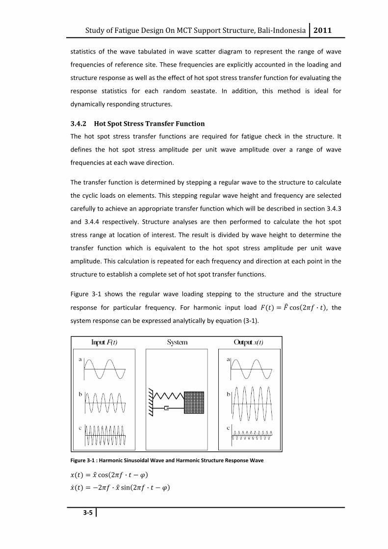
Figure 3‐1 shows the regular wave loading stepping to the structure and the structure
response for particular frequency. For harmonic input load cos 2 · , the
system response can be expressed analytically by equation (3‐1).
Figure 3‐1 : Harmonic Sinusoidal Wave and Harmonic Structure Response Wave
cos 2 ·
2 · sin 2 ·
Study of Fatigue Design On MCT Support Structure, Bali‐Indonesia 2011
3‐6
4 · cos 2 ·
(3‐1)
Where = body displacement [m]
= body velocity [m/s]
= body acceleration [m/s2]
= displacement amplitude [m]
= excitation frequency [Hz]
= time [s]
= phase angle [rad]
By substituting equation (3‐1) to (2‐27) , with replacing by , the system can be re‐
written by equation (3‐2). Once the solution has been found, the structure transfer function
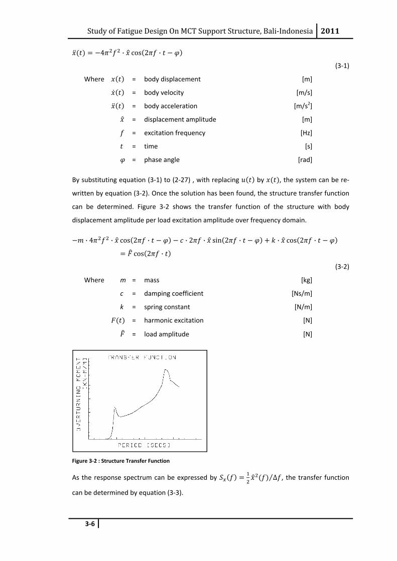
can be determined. Figure 3‐2 shows the transfer function of the structure with body
displacement amplitude per load excitation amplitude over frequency domain.
· 4 · cos 2 · · 2 · sin 2 · · cos 2 ·
cos 2 ·
(3‐2)
Where m = mass [kg]
c = damping coefficient [Ns/m]
k = spring constant [N/m]
= harmonic excitation [N]
= load amplitude [N]
Figure 3‐2 : Structure Transfer Function
As the response spectrum can be expressed by Δ⁄ , the transfer function
can be determined by equation (3‐3).
Study of Fatigue Design On MCT Support Structure, Bali‐Indonesia 2011
3‐7
lim12 Δ
lim · 12 Δ
·
·
(3‐3)
Where = structure response spectrum [m2s]
= excitation spectrum [N2s]
= transfer function of structure [m/N]
3.4.3 Wave Height Selection
The wave selection is aimed to limit the non‐linearity introduced by drag component in the
wave loading. This can be done by using a constant wave steepness which provides a simple
relation between wave height and wave frequency. The wave steepness can be expressed in
equation (3‐4) with typical values in the range of 1:15 to 1:25.
·
21.56
(3‐4)
Where = wave height [m]
= wave steepness [‐]
= wave length [m]
= gravity acceleration ( = 9.81 ) [m/s2]
= wave period [m]
The use of constant wave steepness will introduce unrealistic large wave height at small
frequencies. Therefore, limitation has been given with using minimum wave height of 0.3m
(1 foot) and maximum wave height equal to the design wave height.
3.4.4 Wave Frequency Selection
The wave frequency selection is aimed to set a fine wave response over relevant frequency
range. The followings describe the basis for frequency selection based on structure and
environment characteristics.
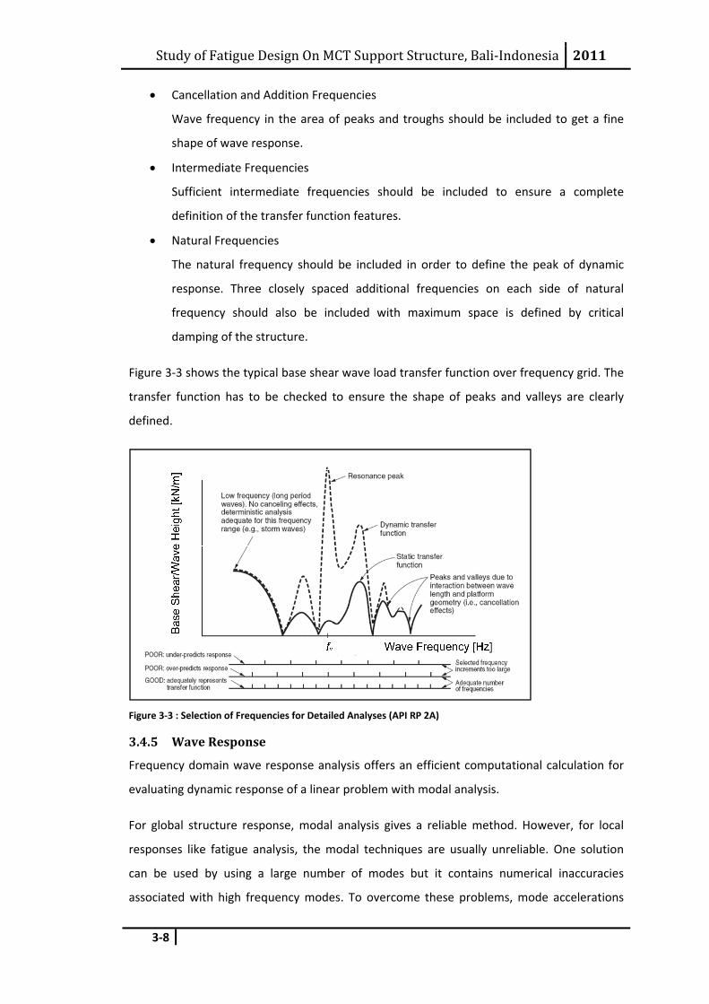
• Minimum and Maximum Frequencies
The minimum and maximum frequency should cover the significant energy of the
seastate.
Study of Fatigue Design On MCT Support Structure, Bali‐Indonesia 2011
3‐8
• Cancellation and Addition Frequencies
Wave frequency in the area of peaks and troughs should be included to get a fine
shape of wave response.
• Intermediate Frequencies
Sufficient intermediate frequencies should be included to ensure a complete
definition of the transfer function features.
• Natural Frequencies
The natural frequency should be included in order to define the peak of dynamic
response. Three closely spaced additional frequencies on each side of natural
frequency should also be included with maximum space is defined by critical
damping of the structure.
Figure 3‐3 shows the typical base shear wave load transfer function over frequency grid. The
transfer function has to be checked to ensure the shape of peaks and valleys are clearly
defined.
Figure 3‐3 : Selection of Frequencies for Detailed Analyses (API RP 2A)
3.4.5 Wave Response
Frequency domain wave response analysis offers an efficient computational calculation for
evaluating dynamic response of a linear problem with modal analysis.
For global structure response, modal analysis gives a reliable method. However, for local
responses like fatigue analysis, the modal techniques are usually unreliable. One solution
can be used by using a large number of modes but it contains numerical inaccuracies
associated with high frequency modes. To overcome these problems, mode accelerations
Study of Fatigue Design On MCT Support Structure, Bali‐Indonesia 2011
3‐9
method is introduced which superimposes the dynamic responses due to limited number of
modes into a full static solution. This method can represent the significant dynamic response
with reliable accuracy and computational efficiency by including a sufficient number of
modes.
The SACS wave response module has capability to use equivalent static load to represent the
loads on structure due to fluid motion including the relative motion between structure and
fluid. The equivalent static load consists of inertia and hydrodynamic loadings which come
from modal acceleration and the fluid‐structure motion respectively. As the high frequency
modes has static response, the dynamic amplification will significantly occur at low
frequency overall structural modes. Thus, the significant inertia loads can be found in this
range. The equivalent static load eliminates large number of modes by adding inertia loading
that has significant dynamic amplification to the actual hydrodynamic loading. In the oil and
gas industry, it is recommended to use this technique if not specified in the design criteria.
3.4.6 Linearization of Nonlinear Wave Loads
The load calculation is based on water particle velocity and acceleration as discussed in
section 2.4. The particle motion can be approached by several theories; however, the Airy
wave linear theory is the most accurate theory to model this linearity. According to Airy
theory, the particle velocities and accelerations are linearly dependent on the wave
amplitude.
The non‐linear wave load is only introduced by drag term of Morison equation as seen on
equation (3‐5) or (2‐10) which shows the square of the velocity in the drag term.
4·
12
· | |
(3‐5)
The total hydrodynamic load and overturning moment on a single pile with uniform
diameter can be determined by integrating and from sea bed to free water surface
elevation as expressed by equation (3‐6).
, ,
, , ·
(3‐6)
Where = total hydrodynamic load [N]
Study of Fatigue Design On MCT Support Structure, Bali‐Indonesia 2011
3‐10
= overturning moment [Nm]
= hydrodynamic inertia load per unit length [N/m]
= hydrodynamic drag load per unit length [N/m]
= water surface [m]
= mean water depth [m]
Simplification of equation (3‐6) can be used by setting the integration from seabed to still
water level 0 . This method discard the drag force acting on pile during the passage of
wave crest but does not affect the inertia load as the maximum load occurs when the wave
surface at zero crossing. Although this condition can be significant at drag dominated term,
it has shown that for this particular application, this simplification is still valid. As the pile
diameter is much smaller than the excitation wave, the governed wave loading is mainly due
to inertia. For less extreme wave condition, fatigue waves, the inertia loading dominates the
total hydrodynamic loading. Therefore the wave induced fatigue will be influenced by linear
inertia wave loading. The magnitude of drag and inertia load and moment can be expressed
by equation (3‐7).
4 · tanh
12
·12 sinh 2
4 · tanh
1 1cosh
1
12
·2
2 1 cosh 24 sinh 2
(3‐7)
Where = inertia load [N]
= drag load [N]
= inertia moment [Nm]
= drag moment [Nm]
= mass water density [kg/m3]
= acceleration of gravity [m/s2]
= wave number [rad/m]
= inertia coefficient [‐]
= drag coefficient [‐]
= diameter of pile [m]
= wave amplitude [m]
Study of Fatigue Design On MCT Support Structure, Bali‐Indonesia 2011
3‐11
3.4.7 Natural Frequency
The natural frequency of the MCT support structure depends on design configuration and
mass at the top of tower. The theoretical frequency should be reviewed and selected
carefully as expressed in equation (2‐29) and described in Figure 2‐21. The position of
natural frequency defines the level of dynamic response. Resonance would occur if the
natural frequency is in the vicinity of excitation frequency of the wave or turbine and might
lead to structure failure. If the natural frequency falls in a valley of the base shear wave load
transfer function, it should be shifted by 5 to 10% to a more conservative location. This can
be done by adjusting the mass or stiffness parameters of the MCT support structure. The
choice of modification depends on the support structure type, mass and soil conditions.
Since the top mass is relatively fixed by turbine manufacturer, the adjustment has to be
made in the stiffness of MCT support structure by changing the diameter of tower and pile.
However, the foundation stiffness modification may sensitive to fatigue analysis.
3.4.8 Shortterm Hot Spot Stress Statistics
After calculating the hot spot stress transfer function for all locations in the structure, the
short‐term statistics of hot spot stress are calculated using standard spectral as described in
section 2.4.2. The short‐term statistics indicates the numbers that the hotspot stress range
exceeds a certain value at one occurrence for a particular approach direction.
The hot spot stress transfer function for a particular location and wave direction are tailored
with the spectrum to calculate the hot spot stress response spectrum for each seastate. The
Root Mean Square (RMS) value and mean period of the hot spot stress response are
determined by integration function of the spectrum and its higher moments. These
components are to be used for probability distribution function of peak value to achieve the
short term statistics of the hot spot stress range.
For narrow banded process, the Rayleigh probability distribution function is normally used,
while Rice probability distribution function is valid for Gaussian random process of any
width. In practice, Rayleigh probability distribution is appropriate for relatively similar waves
and Rice can be used for varies wave data.
Rayleigh Probability Distribution Function
The Rayleigh distribution is based on the zeroth moment of the spectrum as expressed by
equation (3‐8).

Study of Fatigue Design On MCT Support Structure, Bali‐Indonesia 2011
3‐12
1
1
(3‐8)
Where = stress amplitude [N/m2]
= stress range 2 [N/m2]
= zeroth moment of spectrum [‐]
The number of stress ranges per stress range class can be expressed by equation (3‐9).
(3‐9)
Where = number of cycles present at stress range [‐]
= duration of the state [s]
= average period between stress range [s]
Rice Probability Distribution Function
The Rice distribution is based on the zeroth, second and fourth order moment of the
spectrum as expressed by equation (3‐10).
12
1 · ·√1
1√2
1 1
(3‐10)
Where = cumulative prob. of standard normal distribution [‐]
= spectral width parameter [‐]
= second moment of spectrum [‐]
= fourth moment of spectrum [‐]
The number of stress ranges per stress range class can be expressed in equation (3‐11).
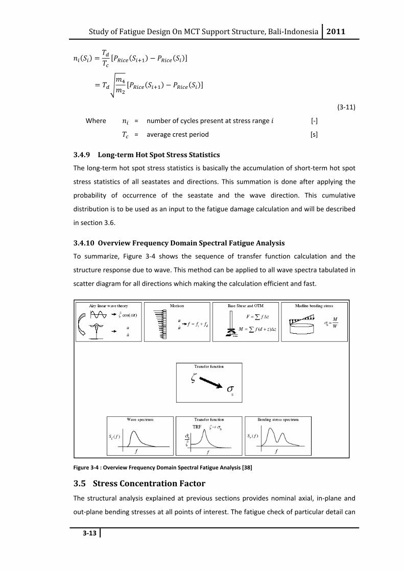
Study of Fatigue Design On MCT Support Structure, Bali‐Indonesia 2011
3‐13
(3‐11)
Where = number of cycles present at stress range [‐]
= average crest period [s]
3.4.9 Longterm Hot Spot Stress Statistics
The long‐term hot spot stress statistics is basically the accumulation of short‐term hot spot
stress statistics of all seastates and directions. This summation is done after applying the
probability of occurrence of the seastate and the wave direction. This cumulative
distribution is to be used as an input to the fatigue damage calculation and will be described
in section 3.6.
3.4.10 Overview Frequency Domain Spectral Fatigue Analysis
To summarize, Figure 3‐4 shows the sequence of transfer function calculation and the
structure response due to wave. This method can be applied to all wave spectra tabulated in
scatter diagram for all directions which making the calculation efficient and fast.
Figure 3‐4 : Overview Frequency Domain Spectral Fatigue Analysis [38]
3.5 Stress Concentration Factor The structural analysis explained at previous sections provides nominal axial, in‐plane and
out‐plane bending stresses at all points of interest. The fatigue check of particular detail can
Study of Fatigue Design On MCT Support Structure, Bali‐Indonesia 2011
3‐14
be performed by adding the local hot spot stress with stress concentration factor (SCF)
which accounts the effect of geometry of the detail on the local stress distribution. Different
SCFs may apply on the nominal stress components depend on the geometry of the detail.
The combination of SCFs and nominal stress components produces the peak hot spot stress.
In addition, the SCFs should be compatible with nominal stresses and S‐N curve.
The stress concentration factors for commonly occurring details are available in standards or
codes. For simple geometry, it can be calculated directly. For more complex connection,
parametric formulae are introduced which derived from model tests or finite element
analyses. In case of unusual connection that does not apply to any codes or standards,
detailed finite element analysis is required to determine the SCF.
The commonly used SCF’s equation is provided by Efthymiou. It consists parametric
equations for T, Y, K, KT and X‐joint configurations under axial load, in‐plane bending and
out‐plane bending. The SCF should be applied to the chord or brace side of the tubular
intersection weld.
The standards or codes of SCF can be found in API RP 2A and DnV RP C203 for other details
like tubular thickness transition.
3.6 Fatigue Endurance
3.6.1 Introduction
From spectral fatigue analysis, the long‐term hot spot stress range statistics has been
produced in form of number of cycles. These statistics are to be used in fatigue endurance
calculation using an appropriate S‐N curve for each connection detail in conjunction with
Miner’s rule for linear accumulation of the fatigue damage. For welded structures, the most
sensitive to fatigue failure are normally associated with the weld itself and the details of the
welds in respect of geometry and welding particulars.
3.6.2 SN Curve
The S‐N curve provides the allowable numbers of cycles failed due to fatigue at particular
stress range. The commonly used standards of S‐N curves can be found in API, Eurocodes
and DnV. For example, API X and X‐prime for simple tubular connections can be found in API
RP 2A. However, the most comprehensive set of S‐N curves can be found in DnV RP C203
which covers a broad range of connection details.

Study of Fatigue Design On MCT Support Structure, Bali‐Indonesia 2011
3‐15
The selection of S‐N curves is based on the direction of applied stresses, the fabrication
method and the inspection method.
Figure 3‐5 : Typical S‐N Curve for Structural Detail
Figure 3‐5 shows the typical S‐N curve for steel material with slope of 3 at lower cycles and
slope of 5 at higher cycles. The stress range and number of cycles axes are in log‐log domain.
3.6.3 Miner’s Rule
The Miner’s rule provides the cumulative fatigue damage calculation for linear approach. It
enables the constant amplitude design of S‐N curves to be applied in the structure exposed
to variable amplitude loadings. The Miner’s rule has the reliability to predict the actual
fatigue lives due to variable amplitude loading, particularly for welded connection. The
fatigue damage ratio based on Miner’s rule is expressed by equation (3‐12).
(3‐12)
Where = cumulative fatigue damage ratio [‐]
= number of cycles present at given stress range [‐]
= allowable number of cycles at given stress range [‐]
= stress range at [kN/m2]
The Miner’s rule states that the detail is considered safe due to fatigue if 1.
The design fatigue life is determined by the inverse of the cumulative fatigue damage ratio
in yearly basis.
1
(3‐13)
Study of Fatigue Design On MCT Support Structure, Bali‐Indonesia 2011
4‐1
4 METHODOLOGY
4.1 Introduction This methodology can be used as general fatigue design of marine current turbine (MCT)
approached by frequency domain analysis. Structure Analysis Computer System (SASC)
ver.5.2 computer programme is used to calculate the fatigue performance of the structure.
Engineering Dynamic, Inc. (EDI) has developed the SACS system of software for offshore
structure engineering applications. SACS consists of several modular structural analysis
programmes which are interface to each other. Further detail of the software can be read on
SACS manual attached to the software.
The fatigue analysis on MCT has not been developed by SACS. Therefore, in this thesis, the
fatigue analysis and calculation are based on experience and expertise engineering
judgement. The methodology is also applied to a range of representative cases which will be
discussed in this chapter.
The overview of MCT design methodology is described in section 4.2 followed by analysis
set‐up for wave induce fatigue and turbine induce fatigue in section 4.3 and 4.4 respectively.
Section 4.5 covers the MCT support structure, section 4.6 explores the environment data
present in the reference site and finally, section 4.7 describes the computer model used in
this thesis.
4.2 Overview of Methodology The methodology for calculating fatigue performance of structure is divided into two
modules of excitation sources. Current flow moves the blades for electricity generation
which causes vibration in the support structure. Excitation from stochastic process of the
wave is the other source in fatigue analysis design. By these specific sources, vibration
module and wave response module in SACS can be used to predict the analytical fatigue
performance of the support structure.
First, the turbine is modelled on a rigid support structure with a constant rotational speed.
Transfer function of this model can be determined by extraction of structure response over
excitation input. Then, wave excitation is modelled including hydrodynamic damping as the
effect of operating turbine. Stress variation due to wave and turbine generated current are
now can be calculated. By assuming the wave and current induced stresses are independent
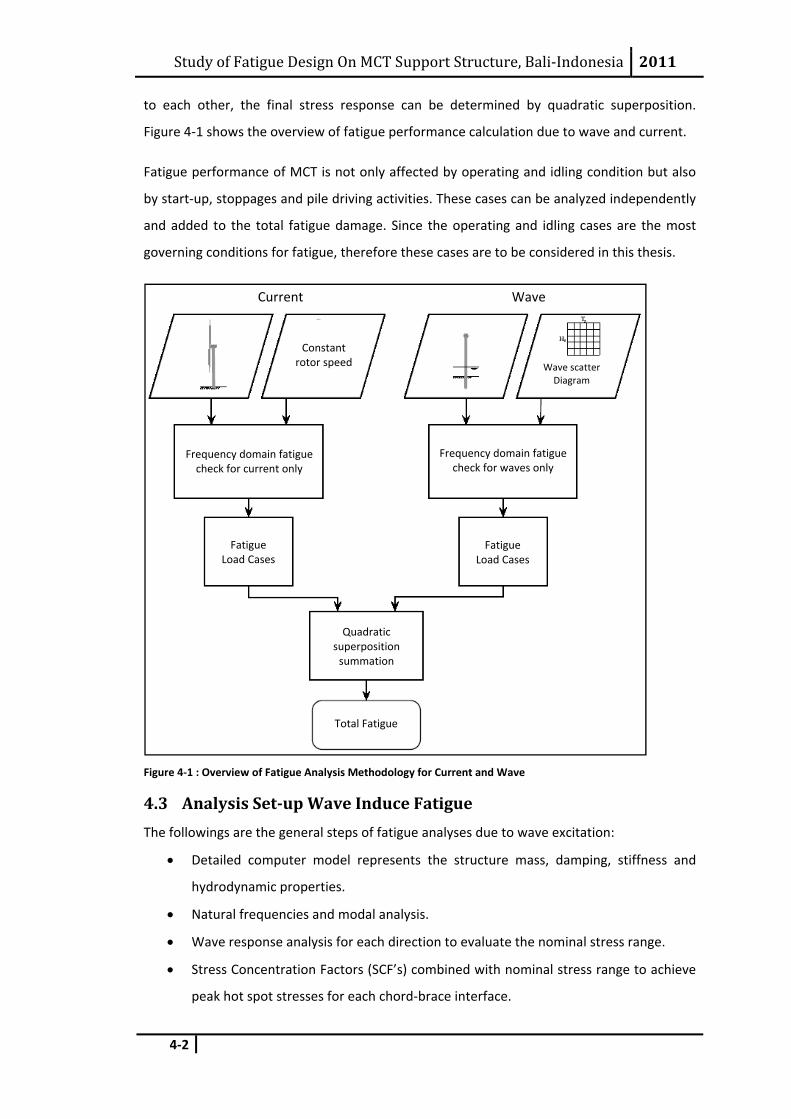
Study of Fatigue Design On MCT Support Structure, Bali‐Indonesia 2011
4‐2
to each other, the final stress response can be determined by quadratic superposition.
Figure 4‐1 shows the overview of fatigue performance calculation due to wave and current.
Fatigue performance of MCT is not only affected by operating and idling condition but also
by start‐up, stoppages and pile driving activities. These cases can be analyzed independently
and added to the total fatigue damage. Since the operating and idling cases are the most
governing conditions for fatigue, therefore these cases are to be considered in this thesis.
Figure 4‐1 : Overview of Fatigue Analysis Methodology for Current and Wave
4.3 Analysis Setup Wave Induce Fatigue The followings are the general steps of fatigue analyses due to wave excitation:
• Detailed computer model represents the structure mass, damping, stiffness and
hydrodynamic properties.
• Natural frequencies and modal analysis.
• Wave response analysis for each direction to evaluate the nominal stress range.
• Stress Concentration Factors (SCF’s) combined with nominal stress range to achieve
peak hot spot stresses for each chord‐brace interface.
Current
Constant rotor speed
Frequency domain fatigue check for current only
Frequency domain fatigue check for waves only
Quadratic superposition summation
Wave
Wave scatter Diagram
Fatigue Load Cases
Fatigue Load Cases
Total Fatigue
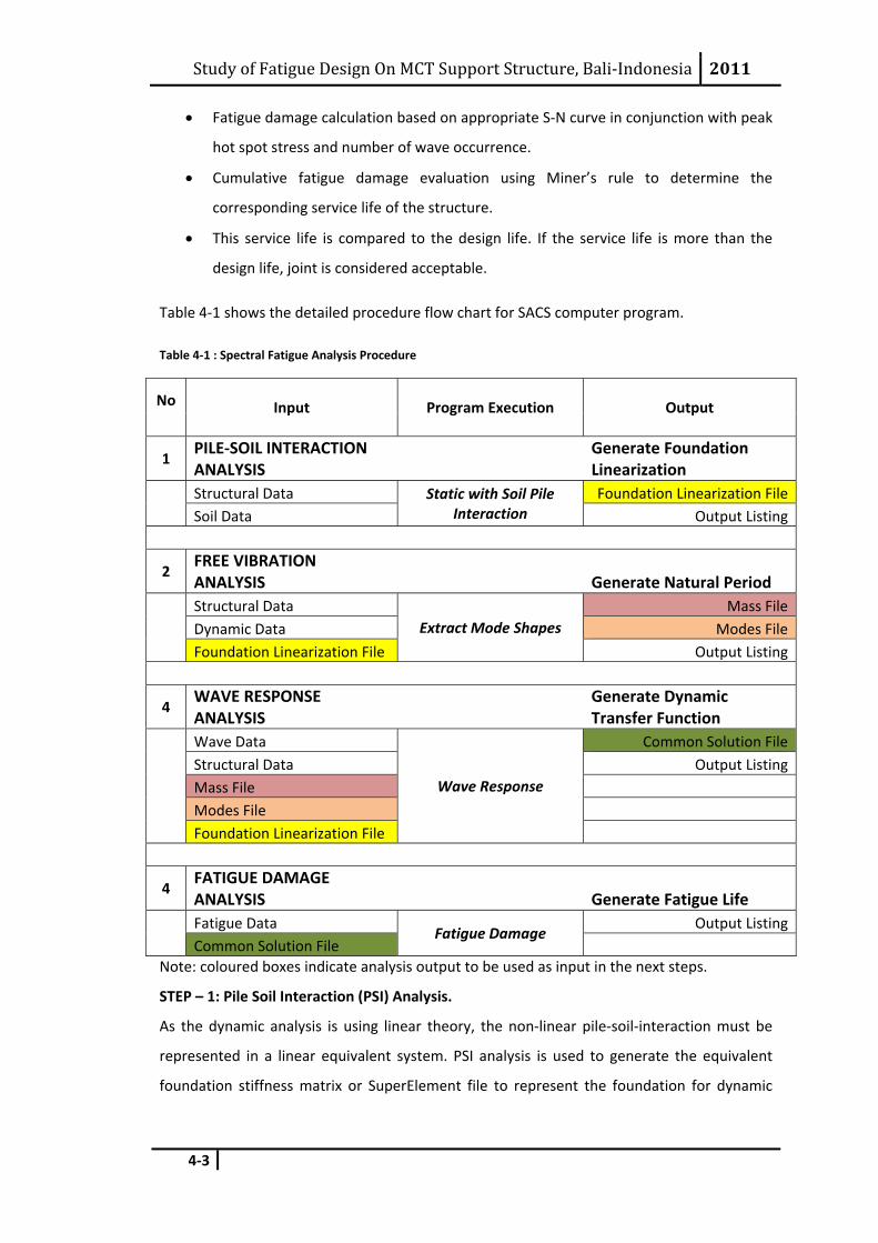
Study of Fatigue Design On MCT Support Structure, Bali‐Indonesia 2011
4‐3
• Fatigue damage calculation based on appropriate S‐N curve in conjunction with peak
hot spot stress and number of wave occurrence.
• Cumulative fatigue damage evaluation using Miner’s rule to determine the
corresponding service life of the structure.
• This service life is compared to the design life. If the service life is more than the
design life, joint is considered acceptable.
Table 4‐1 shows the detailed procedure flow chart for SACS computer program.
Table 4‐1 : Spectral Fatigue Analysis Procedure
No Input Program Execution Output
1 PILE‐SOIL INTERACTION ANALYSIS
Generate Foundation Linearization
Structural Data Static with Soil Pile
Interaction Foundation Linearization File
Soil Data Output Listing
2 FREE VIBRATION ANALYSIS Generate Natural Period
Structural Data Extract Mode Shapes
Mass FileDynamic Data Modes FileFoundation Linearization File Output Listing
4 WAVE RESPONSE ANALYSIS
Generate Dynamic Transfer Function
Wave Data
Wave Response
Common Solution FileStructural Data Output ListingMass File Modes File Foundation Linearization File
4 FATIGUE DAMAGE ANALYSIS Generate Fatigue Life
Fatigue Data
Fatigue Damage Output Listing
Common Solution File Note: coloured boxes indicate analysis output to be used as input in the next steps.
STEP – 1: Pile Soil Interaction (PSI) Analysis.
As the dynamic analysis is using linear theory, the non‐linear pile‐soil‐interaction must be
represented in a linear equivalent system. PSI analysis is used to generate the equivalent
foundation stiffness matrix or SuperElement file to represent the foundation for dynamic

Study of Fatigue Design On MCT Support Structure, Bali‐Indonesia 2011
4‐4
analysis. Since fixed linear foundation is to be applied in analysis, thus this step can be
neglected.
STEP – 2: Free Vibration Analysis
Free vibration analysis is performed to determine the dynamic characteristic of the
structure. This includes natural periods, mode shapes and modal internal load and stress
vectors. This module generates the structural mass for all modelled elements and associate
loadings. In addition, the added mass of entrapped fluid in members is also considered.
STEP – 3: Wave Response
The wave response module is used to compute the dynamic response of the structure
subjected to wave action. The wave response program interacts with the dynamic analysis
program to produce modal response in order to calculate the internal load members. This
internal load on each member is described as Common Solution File (CSF).
From the wave data, the numbers of wave heights with corresponding periods are used to
define the relationship between wave height and stress range. The stress range for each
wave and the number of occurrence is then used to determine fatigue damage.
STEP – 4: Fatigue Damage Analysis
Fatigue is a post‐processing program in SACS to evaluate the structure performance with
respect to fatigue failure. It uses the results of dynamic and wave response analysis to
evaluate the stresses for tubular cross sections around the welded connections. The stresses
are then multiplied by stress concentration factors and stress ranges are evaluated.
The resulting stress ranges are then used to find the damage rates at each of the eight points
of joint tubular cross section by calculating the ratio of the number of occurrences of this
stress range to that which would produce failure as determined from S‐N curve.
4.4 Analysis Setup Turbine Induce Fatigue The fatigue damage due to turbine loading has not been developed in SASC yet. Therefore,
approximation will be made by adopting the above steps and used Engine Vibration Analysis
instead of Wave Response Analysis to evaluate the nominal stress range of the turbine. The
total service life of the structure is evaluated by merging the cumulative fatigue damage
from each analysis.
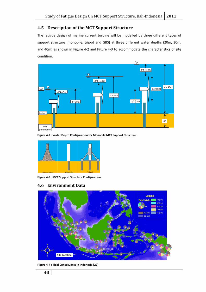
Study of Fatigue Design On MCT Support Structure, Bali‐Indonesia 2011
4‐5
4.5 Description of the MCT Support Structure The fatigue design of marine current turbine will be modelled by three different types of
support structure (monopile, tripod and GBS) at three different water depths (20m, 30m,
and 40m) as shown in Figure 4‐2 and Figure 4‐3 to accommodate the characteristics of site
condition.
Figure 4‐2 : Water Depth Configuration for Monopile MCT Support Structure
Figure 4‐3 : MCT Support Structure Configuration
4.6 Environment Data
Figure 4‐4 : Tidal Constituents in Indonesia [22]
Seabed
Pile penetration
d = 40m
d/2 (typ)
d/2 (typ)
6D
d/4 = 10m
d = 30m
d/4 = 7.5m
d = 20m
d/4 = 5m LAT
Gravity Base Monopile Tripod
Java Island Bali Island
Site Location
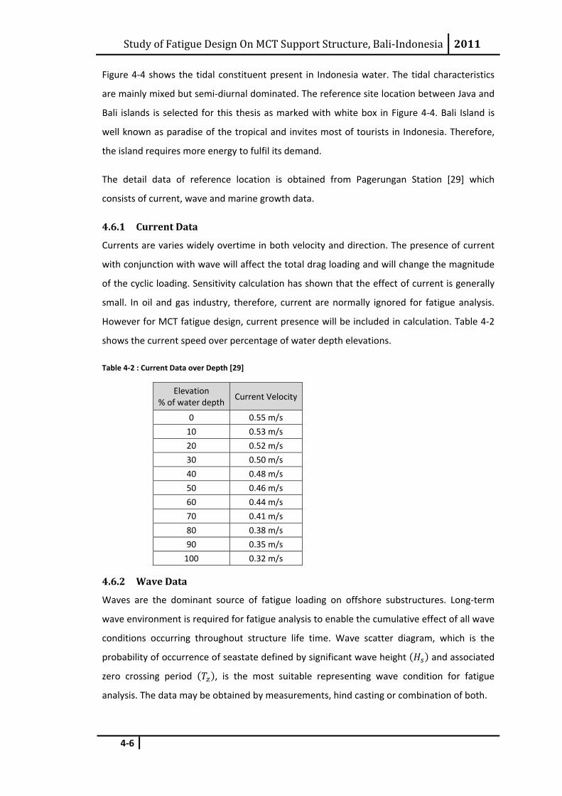
Study of Fatigue Design On MCT Support Structure, Bali‐Indonesia 2011
4‐6
Figure 4‐4 shows the tidal constituent present in Indonesia water. The tidal characteristics
are mainly mixed but semi‐diurnal dominated. The reference site location between Java and
Bali islands is selected for this thesis as marked with white box in Figure 4‐4. Bali Island is
well known as paradise of the tropical and invites most of tourists in Indonesia. Therefore,
the island requires more energy to fulfil its demand.
The detail data of reference location is obtained from Pagerungan Station [29] which
consists of current, wave and marine growth data.
4.6.1 Current Data
Currents are varies widely overtime in both velocity and direction. The presence of current
with conjunction with wave will affect the total drag loading and will change the magnitude
of the cyclic loading. Sensitivity calculation has shown that the effect of current is generally
small. In oil and gas industry, therefore, current are normally ignored for fatigue analysis.
However for MCT fatigue design, current presence will be included in calculation. Table 4‐2
shows the current speed over percentage of water depth elevations.
Table 4‐2 : Current Data over Depth [29]
Elevation % of water depth
Current Velocity
0 0.55 m/s
10 0.53 m/s
20 0.52 m/s
30 0.50 m/s
40 0.48 m/s
50 0.46 m/s
60 0.44 m/s
70 0.41 m/s
80 0.38 m/s
90 0.35 m/s
100 0.32 m/s
4.6.2 Wave Data
Waves are the dominant source of fatigue loading on offshore substructures. Long‐term
wave environment is required for fatigue analysis to enable the cumulative effect of all wave
conditions occurring throughout structure life time. Wave scatter diagram, which is the
probability of occurrence of seastate defined by significant wave height and associated
zero crossing period , is the most suitable representing wave condition for fatigue
analysis. The data may be obtained by measurements, hind casting or combination of both.
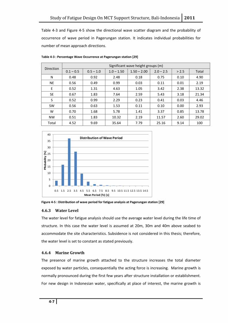
Study of Fatigue Design On MCT Support Structure, Bali‐Indonesia 2011
4‐7
Table 4‐3 and Figure 4‐5 show the directional wave scatter diagram and the probability of
occurrence of wave period in Pagerungan station. It indicates individual probabilities for
number of mean approach directions.
Table 4‐3 : Percentage Wave Occurrence at Pagerungan station [29]
Direction Significant wave height groups (m)
0.1 – 0.5 0.5 – 1.0 1.0 – 1.50 1.50 – 2.00 2.0 – 2.5 > 2.5 Total
N 0.48 0.92 2.48 0.18 0.75 0.10 4.90
NE 0.56 0.49 0.99 0.03 0.11 0.01 2.19
E 0.52 1.31 4.63 1.05 3.42 2.38 13.32
SE 0.67 1.83 7.64 2.59 5.43 3.18 21.34
S 0.52 0.99 2.29 0.23 0.41 0.03 4.46
SW 0.56 0.63 1.53 0.11 0.10 0.00 2.93
W 0.70 1.68 5.78 1.41 3.37 0.85 13.78
NW 0.51 1.83 10.32 2.19 11.57 2.60 29.02
Total 4.52 9.69 35.64 7.79 25.16 9.14 100
Figure 4‐5 : Distribution of wave period for fatigue analysis at Pagerungan station [29]
4.6.3 Water Level
The water level for fatigue analysis should use the average water level during the life time of
structure. In this case the water level is assumed at 20m, 30m and 40m above seabed to
accommodate the site characteristics. Subsidence is not considered in this thesis; therefore,
the water level is set to constant as stated previously.
4.6.4 Marine Growth
The presence of marine growth attached to the structure increases the total diameter
exposed by water particles, consequentially the acting force is increasing. Marine growth is
normally pronounced during the first few years after structure installation or establishment.
For new design in Indonesian water, specifically at place of interest, the marine growth is
0
5
10
15
20
25
30
35
40
0.5 1.5 2.5 3.5 4.5 5.5 6.5 7.5 8.5 9.5 10.5 11.5 12.5 13.5 14.5
PRob
ability [%]
Mean Period (Tz) [s]
Distribution of Wave Period
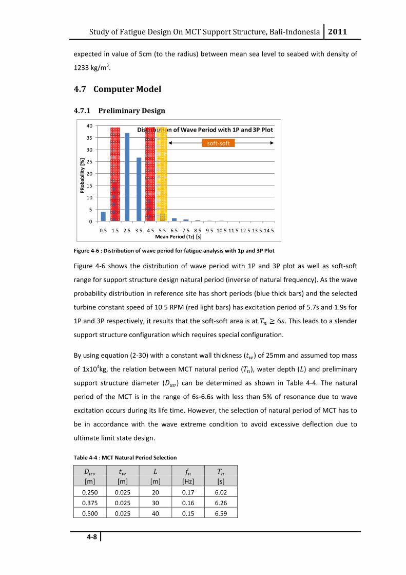
Study of Fatigue Design On MCT Support Structure, Bali‐Indonesia 2011
4‐8
expected in value of 5cm (to the radius) between mean sea level to seabed with density of
1233 kg/m3.
4.7 Computer Model
4.7.1 Preliminary Design
Figure 4‐6 : Distribution of wave period for fatigue analysis with 1p and 3P Plot
Figure 4‐6 shows the distribution of wave period with 1P and 3P plot as well as soft‐soft
range for support structure design natural period (inverse of natural frequency). As the wave
probability distribution in reference site has short periods (blue thick bars) and the selected
turbine constant speed of 10.5 RPM (red light bars) has excitation period of 5.7s and 1.9s for
1P and 3P respectively, it results that the soft‐soft area is at 6 . This leads to a slender
support structure configuration which requires special configuration.
By using equation (2‐30) with a constant wall thickness ( ) of 25mm and assumed top mass
of 1x10⁴kg, the relation between MCT natural period ( ), water depth ( ) and preliminary
support structure diameter ( ) can be determined as shown in Table 4‐4. The natural
period of the MCT is in the range of 6s‐6.6s with less than 5% of resonance due to wave
excitation occurs during its life time. However, the selection of natural period of MCT has to
be in accordance with the wave extreme condition to avoid excessive deflection due to
ultimate limit state design.
Table 4‐4 : MCT Natural Period Selection
[m] [m] [m] [Hz] [s]
0.250 0.025 20 0.17 6.02
0.375 0.025 30 0.16 6.26
0.500 0.025 40 0.15 6.59
0
5
10
15
20
25
30
35
40
0.5 1.5 2.5 3.5 4.5 5.5 6.5 7.5 8.5 9.5 10.5 11.5 12.5 13.5 14.5
PRob
ability [%]
Mean Period (Tz) [s]
Distribution of Wave Period with 1P and 3P Plot
soft‐soft

Study of Fatigue Design On MCT Support Structure, Bali‐Indonesia 2011
4‐9
4.7.2 PileSoilInteraction Analysis
Clamped foundation model with fixity depth of 6D is considered in this thesis as described in
section 2.7. Therefore, the foundation model for MCT support structure is in linear form in
conjunction with the structure model.
4.7.3 Free Vibration Analysis
Specific inputs are required for free vibration analysis as described here after:
• Consistent Mass Option is chosen since it gives better estimated of calculated added
mass.
• The linear foundation of 6D is used for carrying out the free vibration analysis.
• Retained degrees of freedom are specified on all main structural joints so as to
obtain all the modes having higher mass participation factors.
• The pile is kept flooded for entrapped water mass in the natural frequency
calculation.
• A total of 3 modes have been extracted to participate in spectral analysis.
• Added mass coefficient specified is equal to 1.0.
• The weight density of all members has been increased by 10% to account for
miscellaneous weight contingency.
4.7.4 Fatigue Wave Climate
• Total number of wave used in fatigue analysis is 18519217 based on report
“Final report of Metocean Design Criteria for General Kangean Block Area” by PT LAPI ITB, 29 August 2005. [29].
• Airy theory has been used to evaluate the hydrodynamic loading due to fatigue
waves.
• A total of 12 wave directions is chosen to carry out fatigue analysis
4.7.5 Wave Response Analysis
By initiating the “Wave Response” module of SACS the wave response analysis is performed.
The member hydrodynamic loads and member inertia loads due to the structural
acceleration are computed simultaneously at every wave step position by using the model
analysis method. A total of 3 modes computed from free vibration analysis has been used
for obtaining the member inertial loads.
Cd and Cm are adopted from API RP 2A are specified below:
• For fouled members = 0.8 and = 2.00
• For clean members = 0.5 and = 2.00

Study of Fatigue Design On MCT Support Structure, Bali‐Indonesia 2011
4‐10
To account for anodes and other non‐modelled members, the increase in drag and inertia
coefficient must be assessed, generally taken as 5% or as specified in the design criteria.
4.7.6 Fatigue Analysis
After obtaining the member end nominal stress, the fatigue analysis module of SACS is
activated to carry out Joint fatigue analysis.
The following are the important data considered for Fatigue Analysis.
• S‐N curves of DNV curve D, F, F3 and API‐X Prime Curve for Estimation of Joint
Fatigue Lives.
• Joint SCF has been computed by using formula as suggested by Efthymiou and is
load path dependent. Joint SCF obtained by using this option are observed to be on
conservative side.
• The Design Fatigue Life of joint is set to 20 years as a standard life design taken from
offshore wind turbine.
• Life safety factor is set to 4.0 (see section 3.3.5).
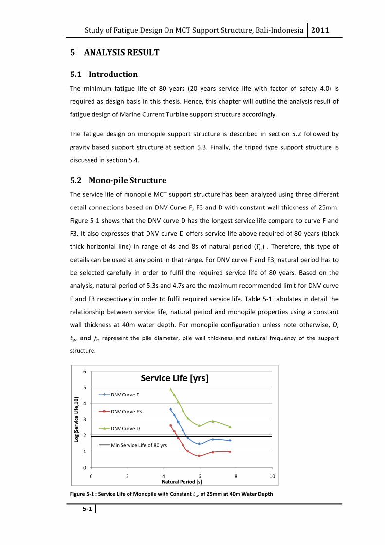
Study of Fatigue Design On MCT Support Structure, Bali‐Indonesia 2011
5‐1
5 ANALYSIS RESULT
5.1 Introduction The minimum fatigue life of 80 years (20 years service life with factor of safety 4.0) is
required as design basis in this thesis. Hence, this chapter will outline the analysis result of
fatigue design of Marine Current Turbine support structure accordingly.
The fatigue design on monopile support structure is described in section 5.2 followed by
gravity based support structure at section 5.3. Finally, the tripod type support structure is
discussed in section 5.4.
5.2 Monopile Structure The service life of monopile MCT support structure has been analyzed using three different
detail connections based on DNV Curve F, F3 and D with constant wall thickness of 25mm.
Figure 5‐1 shows that the DNV curve D has the longest service life compare to curve F and
F3. It also expresses that DNV curve D offers service life above required of 80 years (black
thick horizontal line) in range of 4s and 8s of natural period ( ) . Therefore, this type of
details can be used at any point in that range. For DNV curve F and F3, natural period has to
be selected carefully in order to fulfil the required service life of 80 years. Based on the
analysis, natural period of 5.3s and 4.7s are the maximum recommended limit for DNV curve
F and F3 respectively in order to fulfil required service life. Table 5‐1 tabulates in detail the
relationship between service life, natural period and monopile properties using a constant
wall thickness at 40m water depth. For monopile configuration unless note otherwise, D,
and represent the pile diameter, pile wall thickness and natural frequency of the support
structure.
Figure 5‐1 : Service Life of Monopile with Constant of 25mm at 40m Water Depth
0
1
2
3
4
5
6
0 2 4 6 8 10
Log (Service Life
,10)
Natural Period [s]
Service Life [yrs]
DNV Curve F
DNV Curve F3
DNV Curve D
Min Service Life of 80 yrs
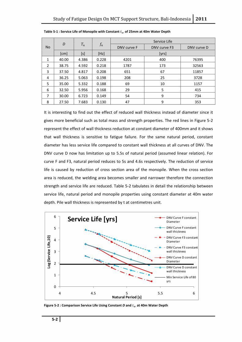
Study of Fatigue Design On MCT Support Structure, Bali‐Indonesia 2011
5‐2
Table 5‐1 : Service Life of Monopile with Constant of 25mm at 40m Water Depth
No D
Service Life
DNV curve F DNV curve F3 DNV curve D
[cm] [s] [Hz] [yrs]
1 40.00 4.386 0.228 4201 400 76395
2 38.75 4.592 0.218 1787 173 32563
3 37.50 4.817 0.208 651 67 11857
4 36.25 5.063 0.198 208 25 3728
5 35.00 5.332 0.188 69 10 1157
6 32.50 5.956 0.168 29 5 415
7 30.00 6.723 0.149 54 9 734
8 27.50 7.683 0.130 47 9 353
It is interesting to find out the effect of reduced wall thickness instead of diameter since it
gives more beneficial such as total mass and strength properties. The red lines in Figure 5‐2
represent the effect of wall thickness reduction at constant diameter of 400mm and it shows
that wall thickness is sensitive to fatigue failure. For the same natural period, constant
diameter has less service life compared to constant wall thickness at all curves of DNV. The
DNV curve D now has limitation up to 5.5s of natural period (assumed linear relation). For
curve F and F3, natural period reduces to 5s and 4.6s respectively. The reduction of service
life is caused by reduction of cross section area of the monopile. When the cross section
area is reduced, the welding area becomes smaller and narrower therefore the connection
strength and service life are reduced. Table 5‐2 tabulates in detail the relationship between
service life, natural period and monopile properties using constant diameter at 40m water
depth. Pile wall thickness is represented by t at centimetres unit.
Figure 5‐2 : Comparison Service Life Using Constant D and at 40m Water Depth
0
1
2
3
4
5
6
4 4.5 5 5.5 6
Log (Service Life
,10)
Natural Period [s]
Service Life [yrs] DNV Curve F constant Diameter
DNV Curve F constant wall thickness
DNV Curve F3 constant Diameter
DNV Curve F3 constant wall thickness
DNV Curve D constant Diameter
DNV Curve D constant wall thickness
Min Service Life of 80 yrs
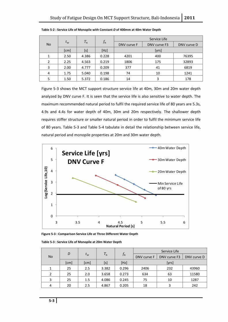
Study of Fatigue Design On MCT Support Structure, Bali‐Indonesia 2011
5‐3
Table 5‐2 : Service Life of Monopile with Constant D of 400mm at 40m Water Depth
No
Service Life
DNV curve F DNV curve F3 DNV curve D
[cm] [s] [Hz] [yrs]
1 2.50 4.386 0.228 4201 400 76395
2 2.25 4.563 0.219 1806 175 32893
3 2.00 4.777 0.209 377 41 6819
4 1.75 5.040 0.198 74 10 1241
5 1.50 5.372 0.186 14 3 178
Figure 5‐3 shows the MCT support structure service life at 40m, 30m and 20m water depth
analyzed by DNV curve F. It is seen that the service life is also sensitive to water depth. The
maximum recommended natural period to fulfil the required service life of 80 years are 5.3s,
4.9s and 4.4s for water depth of 40m, 30m and 20m respectively. The shallower depth
requires stiffer structure or smaller natural period in order to fulfil the minimum service life
of 80 years. Table 5‐3 and Table 5‐4 tabulate in detail the relationship between service life,
natural period and monopile properties at 20m and 30m water depth.
Figure 5‐3 : Comparison Service Life at Three Different Water Depth
Table 5‐3 : Service Life of Monopile at 20m Water Depth
No D
Service Life
DNV curve F DNV curve F3 DNV curve D
[cm] [cm] [s] [Hz] [yrs]
1 25 2.5 3.382 0.296 2406 232 43960
2 25 2.0 3.658 0.273 634 63 11580
3 25 1.5 4.086 0.245 75 10 1287
4 20 2.5 4.867 0.205 18 3 242
0
1
2
3
4
5
6
3 3.5 4 4.5 5 5.5 6
Log (Service Life
,10)
Natural Period [s]
Service Life [yrs] DNV Curve F
40m Water Depth
30m Water Depth
20m Water Depth
Min Service Life of 80 yrs
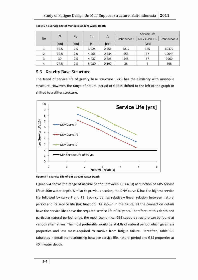
Study of Fatigue Design On MCT Support Structure, Bali‐Indonesia 2011
5‐4
Table 5‐4 : Service Life of Monopile at 30m Water Depth
No D
Service Life
DNV curve F DNV curve F3 DNV curve D
[cm] [cm] [s] [Hz] [yrs]
1 32.5 2.5 3.924 0.255 3817 365 69377
2 32.5 2.0 4.265 0.234 553 57 10044
3 30 2.5 4.437 0.225 548 57 9960
4 27.5 2.5 5.080 0.197 38 6 598
5.3 Gravity Base Structure The trend of service life of gravity base structure (GBS) has the similarity with monopile
structure. However, the range of natural period of GBS is shifted to the left of the graph or
shifted to a stiffer structure.
Figure 5‐4 : Service Life of GBS at 40m Water Depth
Figure 5‐4 shows the range of natural period (between 1.6s‐4.8s) as function of GBS service
life at 40m water depth. Similar to previous section, the DNV curve D has the highest service
life followed by curve F and F3. Each curve has relatively linear relation between natural
period and its service life (log function). As shown in the figure, all the connection details
have the service life above the required service life of 80 years. Therefore, at this depth and
particular natural period range, the most economical GBS support structure can be found at
various alternatives. The most preferable would be at 4.8s of natural period which gives less
properties and less mass required to survive from fatigue failure. Hereafter, Table 5‐5
tabulates in detail the relationship between service life, natural period and GBS properties at
40m water depth.
0
1
2
3
4
5
6
7
8
9
10
0 1 2 3 4 5 6
Log (Service Life
,10)
Natural Period [s]
Service Life [yrs]
DNV Curve F
DNV Curve F3
DNV Curve D
Min Service Life of 80 yrs
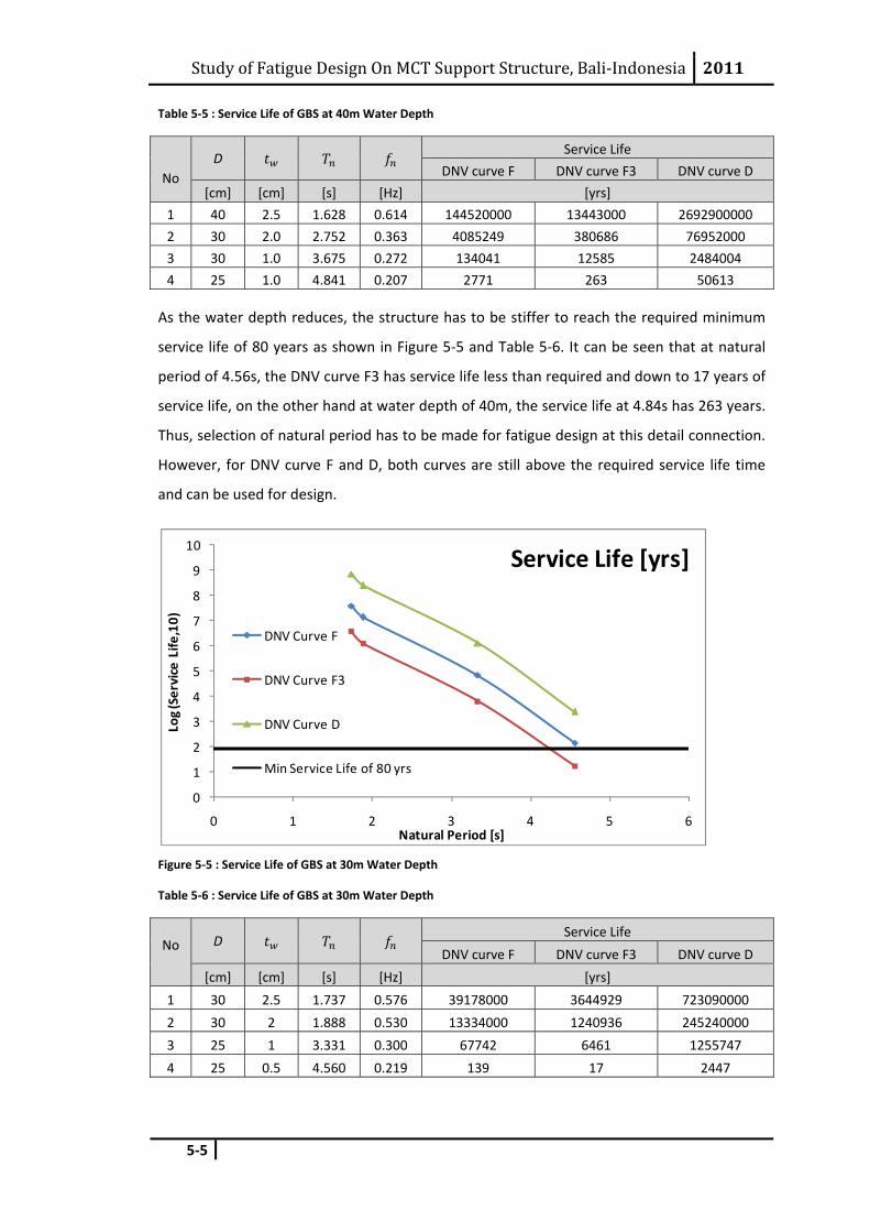
Study of Fatigue Design On MCT Support Structure, Bali‐Indonesia 2011
5‐5
Table 5‐5 : Service Life of GBS at 40m Water Depth
No D
Service Life
DNV curve F DNV curve F3 DNV curve D
[cm] [cm] [s] [Hz] [yrs]
1 40 2.5 1.628 0.614 144520000 13443000 2692900000
2 30 2.0 2.752 0.363 4085249 380686 76952000
3 30 1.0 3.675 0.272 134041 12585 2484004
4 25 1.0 4.841 0.207 2771 263 50613
As the water depth reduces, the structure has to be stiffer to reach the required minimum
service life of 80 years as shown in Figure 5‐5 and Table 5‐6. It can be seen that at natural
period of 4.56s, the DNV curve F3 has service life less than required and down to 17 years of
service life, on the other hand at water depth of 40m, the service life at 4.84s has 263 years.
Thus, selection of natural period has to be made for fatigue design at this detail connection.
However, for DNV curve F and D, both curves are still above the required service life time
and can be used for design.
Figure 5‐5 : Service Life of GBS at 30m Water Depth
Table 5‐6 : Service Life of GBS at 30m Water Depth
No D Service Life
DNV curve F DNV curve F3 DNV curve D
[cm] [cm] [s] [Hz] [yrs]
1 30 2.5 1.737 0.576 39178000 3644929 723090000
2 30 2 1.888 0.530 13334000 1240936 245240000
3 25 1 3.331 0.300 67742 6461 1255747
4 25 0.5 4.560 0.219 139 17 2447
0
1
2
3
4
5
6
7
8
9
10
0 1 2 3 4 5 6
Log (Service Life
,10)
Natural Period [s]
Service Life [yrs]
DNV Curve F
DNV Curve F3
DNV Curve D
Min Service Life of 80 yrs
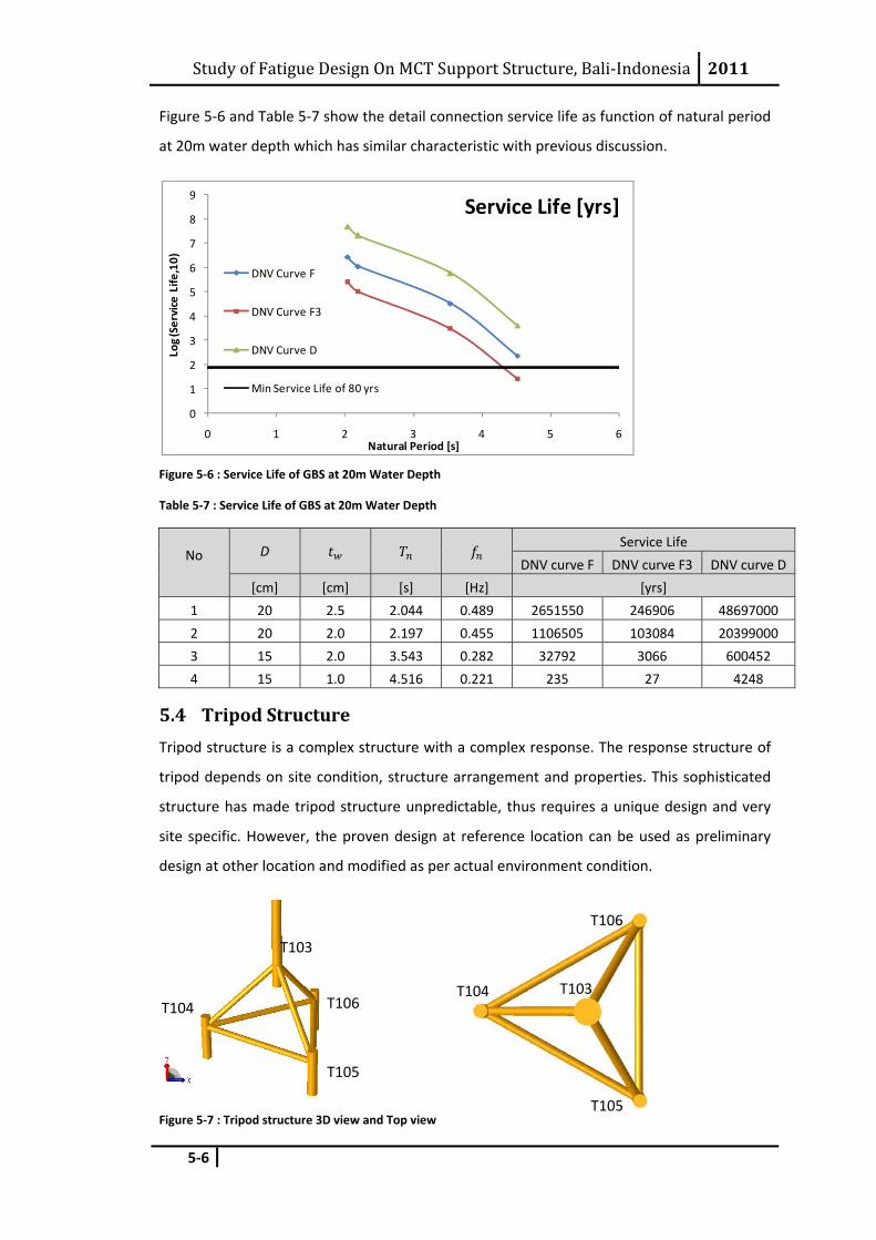
Study of Fatigue Design On MCT Support Structure, Bali‐Indonesia 2011
5‐6
Figure 5‐6 and Table 5‐7 show the detail connection service life as function of natural period
at 20m water depth which has similar characteristic with previous discussion.
Figure 5‐6 : Service Life of GBS at 20m Water Depth
Table 5‐7 : Service Life of GBS at 20m Water Depth
No D Service Life
DNV curve F DNV curve F3 DNV curve D
[cm] [cm] [s] [Hz] [yrs]
1 20 2.5 2.044 0.489 2651550 246906 48697000
2 20 2.0 2.197 0.455 1106505 103084 20399000
3 15 2.0 3.543 0.282 32792 3066 600452
4 15 1.0 4.516 0.221 235 27 4248
5.4 Tripod Structure Tripod structure is a complex structure with a complex response. The response structure of
tripod depends on site condition, structure arrangement and properties. This sophisticated
structure has made tripod structure unpredictable, thus requires a unique design and very
site specific. However, the proven design at reference location can be used as preliminary
design at other location and modified as per actual environment condition.
Figure 5‐7 : Tripod structure 3D view and Top view
0
1
2
3
4
5
6
7
8
9
0 1 2 3 4 5 6
Log (Service Life
,10)
Natural Period [s]
Service Life [yrs]
DNV Curve F
DNV Curve F3
DNV Curve D
Min Service Life of 80 yrs
T103
T104
T105
T106 T103 T104
T105
T106
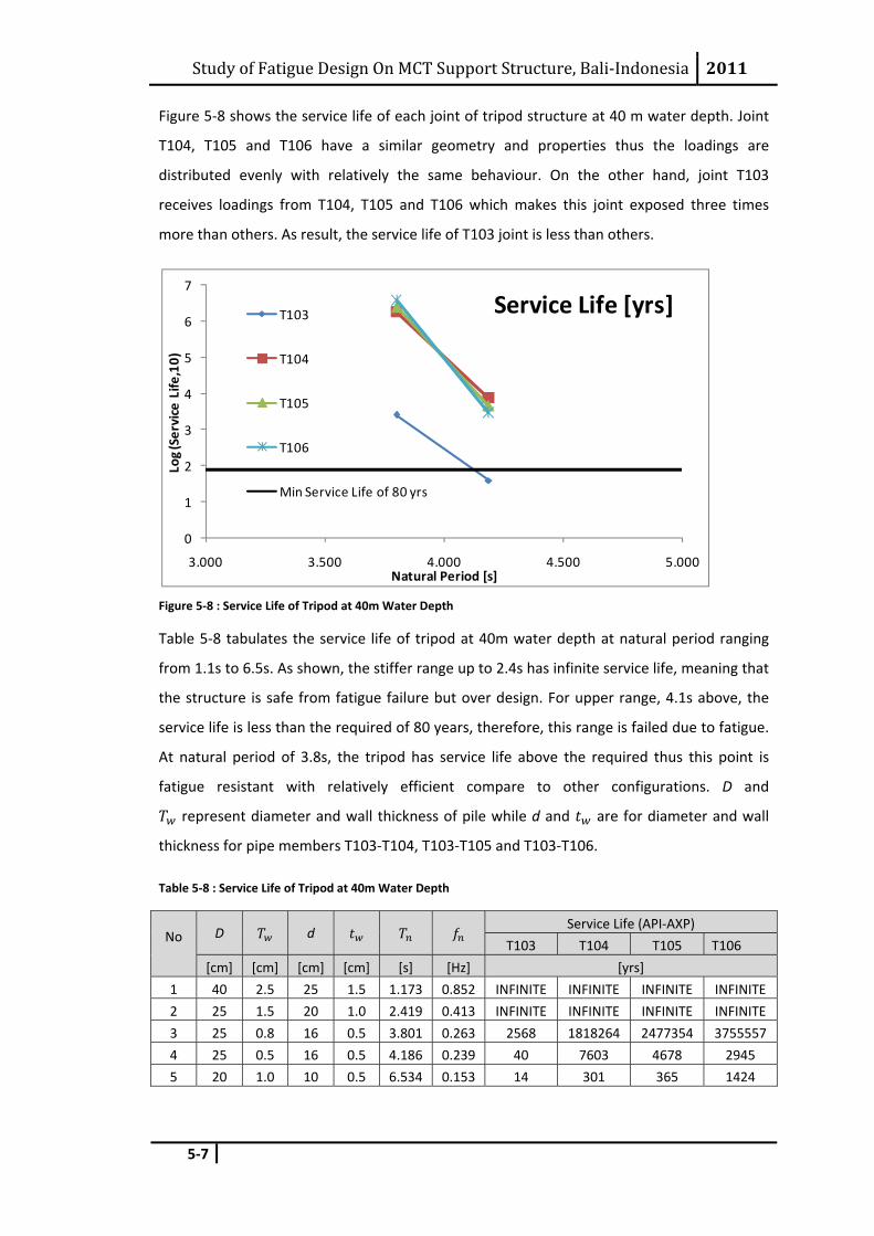
Study of Fatigue Design On MCT Support Structure, Bali‐Indonesia 2011
5‐7
Figure 5‐8 shows the service life of each joint of tripod structure at 40 m water depth. Joint
T104, T105 and T106 have a similar geometry and properties thus the loadings are
distributed evenly with relatively the same behaviour. On the other hand, joint T103
receives loadings from T104, T105 and T106 which makes this joint exposed three times
more than others. As result, the service life of T103 joint is less than others.
Figure 5‐8 : Service Life of Tripod at 40m Water Depth
Table 5‐8 tabulates the service life of tripod at 40m water depth at natural period ranging
from 1.1s to 6.5s. As shown, the stiffer range up to 2.4s has infinite service life, meaning that
the structure is safe from fatigue failure but over design. For upper range, 4.1s above, the
service life is less than the required of 80 years, therefore, this range is failed due to fatigue.
At natural period of 3.8s, the tripod has service life above the required thus this point is
fatigue resistant with relatively efficient compare to other configurations. D and
represent diameter and wall thickness of pile while d and are for diameter and wall
thickness for pipe members T103‐T104, T103‐T105 and T103‐T106.
Table 5‐8 : Service Life of Tripod at 40m Water Depth
No D d Service Life (API‐AXP)
T103 T104 T105 T106
[cm] [cm] [cm] [cm] [s] [Hz] [yrs]
1 40 2.5 25 1.5 1.173 0.852 INFINITE INFINITE INFINITE INFINITE
2 25 1.5 20 1.0 2.419 0.413 INFINITE INFINITE INFINITE INFINITE
3 25 0.8 16 0.5 3.801 0.263 2568 1818264 2477354 3755557
4 25 0.5 16 0.5 4.186 0.239 40 7603 4678 2945
5 20 1.0 10 0.5 6.534 0.153 14 301 365 1424
0
1
2
3
4
5
6
7
3.000 3.500 4.000 4.500 5.000
Log (Service Life
,10)
Natural Period [s]
Service Life [yrs]T103
T104
T105
T106
Min Service Life of 80 yrs
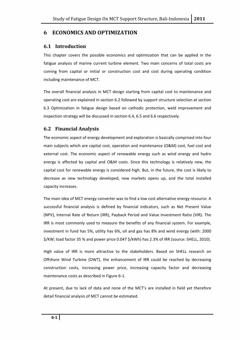
Study of Fatigue Design On MCT Support Structure, Bali‐Indonesia 2011
6‐1
6 ECONOMICS AND OPTIMIZATION
6.1 Introduction This chapter covers the possible economics and optimization that can be applied in the
fatigue analysis of marine current turbine element. Two main concerns of total costs are
coming from capital or initial or construction cost and cost during operating condition
including maintenance of MCT.
The overall financial analysis in MCT design starting from capital cost to maintenance and
operating cost are explained in section 6.2 followed by support structure selection at section
6.3 Optimization in fatigue design based on cathodic protection, weld improvement and
inspection strategy will be discussed in section 6.4, 6.5 and 6.6 respectively.
6.2 Financial Analysis The economic aspect of energy development and exploration is basically comprised into four
main subjects which are capital cost, operation and maintenance (O&M) cost, fuel cost and
external cost. The economic aspect of renewable energy such as wind energy and hydro
energy is affected by capital and O&M costs. Since this technology is relatively new, the
capital cost for renewable energy is considered high. But, in the future, the cost is likely to
decrease as new technology developed, new markets opens up, and the total installed
capacity increases.
The main idea of MCT energy converter was to find a low cost alternative energy resource. A
successful financial analysis is defined by financial indicators, such as Net Present Value
(NPV), Internal Rate of Return (IRR), Payback Period and Value Investment Ratio (VIR). The
IRR is most commonly used to measure the benefits of any financial system. For example,
investment in fund has 5%, utility has 6%, oil and gas has 8% and wind energy (with: 2000
$/KW; load factor 35 % and power price 0.047 $/kWh) has 2.3% of IRR (source: SHELL, 2010).
High value of IRR is more attractive to the stakeholders. Based on SHELL research on
Offshore Wind Turbine (OWT), the enhancement of IRR could be reached by decreasing
construction costs, increasing power price, increasing capacity factor and decreasing
maintenance costs as described in Figure 6‐1.
At present, due to lack of data and none of the MCT’s are installed in field yet therefore
detail financial analysis of MCT cannot be estimated.
Study of Fatigue Design On MCT Support Structure, Bali‐Indonesia 2011
6‐2
Figure 6‐1 : IRR Sensitivity of Offshore Wind Farm (Shell, 2010)
6.3 Support Structure Selection The analysis result from previous chapter shows that each MCT support structure has their
own advantage and limitation. Discussion on advantages and limitations are outlined in this
section.
6.3.1 Monopile Structure
Monopile type structures are appropriate for calm environment of shallow or intermediate
water level (up to 30m depth) with soft soil characteristics such as clay and sand. The single
pile with slender configuration makes monopile structures have relatively large natural
period to keep it economically profitable. This excessive natural period is prone to dynamic
responses and resonance. For Bali strait, per year chance of resonance is up to 9% if the
natural period is set at 4.5 second (see Figure 4‐6). However, the effect of resonance can be
reduced by the hydrodynamic damping of the rotating turbine [38]. On the other hand,
monopile structures can be installed in soft soil characteristics by conventional pile driving
and boring technique. Another note for monopile structures are the effect of excessive
deflection at the top of structure and should be safe in service limit state (SLS) point of view.
6.3.2 Gravity Base Structure
Gravity base structures are appropriate for intermediate (20m to 80m) water depth with
hard or rocky soil characteristics. The hardness of soil characteristics makes it impossible and
not economical to bore or drive, thus the foundation of GBS is held in place by gravity and

Study of Fatigue Design On MCT Support Structure, Bali‐Indonesia 2011
6‐3
often built in with tanks or cells which can be used to control the buoyancy of the finished
GBS. Soil or foundation preparation is also required at relatively large area before placing
GBS into its position.
For Bali strait which is covered by hard coral reef, GBS is suitable to be used. This stiff
structure has bigger strength resistance and has relatively small deflection at the top of
structure. In addition, GBS offers less material cost compare to monopile and tripod type
structures. However, the coral reef area that is converted into GBS foundation has to be
analyzed carefully in accordance with Environment Impact Assessment.
6.3.3 Tripod Structure
Tripod structures are appropriate for intermediate (20m to 80m) water depth with soft soil
characteristics. This structure is the extension of monopile structure with additional three
legs to accommodate stiffness and strength of the structure. In practice, tripod structures
have the strength of GBS in form of monopile structure.
For Bali strait which has soft soil at seabed combined with rocky soil at certain depth below;
tripod structures offer an economical option. The combination of soil friction and bearing tip
leads into a rigid foundation. Thus, the structure becomes stiffer and less affected by fatigue
failure. However, installation procedure has to be considered carefully since it requires pile
driving or boring in the vicinity of coral reef including EIA assessment.
6.4 Cathodic Protection Steel structures submerged in water are susceptible to corrosion. The fatigue design of steel
structures submerged in water is assumed to be adequately protected by a cathodic
protection system. Four methods of cathodic protection can be applied in order to fulfil the
requirements, which are:
• Corrosion allowance, adding extra reserve wall thickness to compensate steel consumption.
• Protective coating, special painting to prevent corrosion, applied in vicinity of dynamically changing environment such as in the water surface area.
• Impressed current, active electrical current to prevent electrochemical process of corrosion at submerged steel.
• Anodes, sacrificial material creating electrochemical process to prevent corrosion at submerged steel.
In oil and gas industry, anodes and protective coating are the most commonly used cathodic
protection system for continuously submerged steel material and area at water surface
elevation respectively. Numbers or anodes should be calculated accordingly due to the
Study of Fatigue Design On MCT Support Structure, Bali‐Indonesia 2011
6‐4
needs of protection. Otherwise, overprotection by using excessive anodes can cause
hydrogen production which can lead to embrittlement and significantly reduce the fatigue
lives. Minimal production of hydrogen can be expected by using conventional aluminium
and zinc anodes for normal steel structures. If, for instance, magnesium anode or higher
strength steel (yield stress over 400 MPa) is used, the threat from hydrogen embrittlement
might occur and therefore it should be examined.
6.5 Weld Improvement Improvement in fatigue life is achieved by grinding weld technique. However this technique
should not be used during design phase because grinding is more expensive compare to
conventional welding. Redesign should be conducted if inadequate fatigue lives occur at
design phase. On the other hand, if fatigue problem occurs during construction or operating
condition and redesign option is not feasible, weld grinding may be used.
To be noted that ground weld improves the fatigue life due to increment of the initiation
time of a defect without improvement of propagation time and therefore the early warning
of crack development is less pronounced.
6.6 Inspection Strategy Analytical prediction for structure fatigue performance provides valuable input for
inspection strategy, especially for submerged structures. The strategy is not only based on
fatigue criteria but also other things such as weather and current speed. However, for new
structure design, a comfortable margin in calculation design fatigue lives provides a cost
effective investment compared to marginal design which requires more extensive fatigue
inspection.
For existing structures with low analytical fatigue lives, the inspection interval may be
updated based on a good in‐service fatigue performance. An assessment of fatigue crack
growth behaviour for welded connection shows that the time for a defect to grow to a size
that reliably detected by practical underwater inspection technique is less than half of the
time for through thickness crack development. This means that an early warning of crack
growth is introduced as the remaining life is at least equal to the initiation period up to time
of detectable size. If defect free is shown by a connection after given service period, the
remaining life will normally be at least equal to the service life to date. And if the updated
service life is significantly over the analytical fatigue life, it means that the analysis has more
conservative value and therefore the inspection interval may be increased accordingly.

Study of Fatigue Design On MCT Support Structure, Bali‐Indonesia 2011
7‐1
7 CONCLUSION AND RECOMMENDATION
7.1 Conclusion After conducting this study, the main conclusions drawn are summarised in the following:
1. Indonesia has many potential tidal energy resources. However, in this thesis, reference
site between Java and Bali islands is selected in order to support tourism in Bali Island
which requires more energy supply.
2. At the reference site, the frequency‐based methodology with two independent
approach of fatigue loading (wave and current induce turbine) is able to simulate the
fatigue damage calculation.
3. The simulation of fatigue damage comprises three different support structures
(monopile, gravity based and tripod) at three different water depth (20, 30 and 40
meters). Those simulations are selected in regards to find out the most effective support
structure based on production cost, construction and maintenance.
4. The lower wave height and shorter wave period derives the inertia component of wave
loading more important in fatigue analysis compare to extreme storm analysis.
Therefore, selection of inertia coefficients and equivalent volumes for members and in
particular for complex assemblies requires careful attention.
5. The fatigue damage analysis shows that DNV curve D has the longest service life
compare to curve F followed by curve F3. This curve selection is based on connection
details design at the MCT support structure.
6. At the same structure natural period, properties with smaller cross section area and
inertia have less service life. The cross section area and inertia of particular connection
represent the welding area, therefore, less cross section properties derive less fatigue
strength.
7. The service life is also sensitive to water depth. The shallower water depth requires
stiffer structure or smaller natural period in order to fulfil the minimum service life of 80
years.
8. The study of fatigue design on MCT support structure in Bali Strait shows that the
fatigue life design has many property alternatives in order to fulfil required service life of
80 years (20 years design life with factor of safety 4.0). For example, from 400mm pile
diameter x 20mm wall thickness of monopile structure using DNV curve F connection
detail at 40m water depth to 250mm pile diameter x 10mm wall thickness of gravity
base structure (GBS) using DNV curve F3 connection detail at 40m water depth.
Study of Fatigue Design On MCT Support Structure, Bali‐Indonesia 2011
7‐2
9. Contrary to the offshore wind turbine with natural period at soft‐soft range, the
recommended natural period range for MCT is placed at soft‐stiff range. This because of
the MCT support structure requires stiffer and more compact structure as they are
exposed to a more severe loading compare to OWT. The operating turbine exposed to
wave and current are the main cause of this difference. It provides larger catching area
hence a larger wave and current loading occur at this stage.
10. Each type of MCT support structure has its own benefits. Based on experiences in the oil
and gas exploration industry, monopile support structure is appropriate for shallow
water with soft soil characteristic (clay and sand). GBS support structure is suitable for
intermediate water depth at rocky or hard soil characteristic. And tripod support
structure is recommended for intermediate water depth at soft soil characteristic (clay
and sand). For Bali strait, GBS and tripod structure are suitable in regards of site soil
characteristics (hard soil and combination of soft‐hard soil).
11. The methodology has been tested for three different type of support structure. It shows
that this methodology can be used as general guidance for fatigue design of MCT
support structure.
12. Although the fatigue design for Bali strait has service life above the required life time,
however for detailed design, a complete and comprehensive environment data (wave,
current and soil) is required to conduct a proper fatigue design assessment.
13. Fatigue design is a unique design for a particular location at particular environment data
(wave, current and soil). Therefore, It is only valid for particular location and cannot be
generalized.
7.2 Recommendation The study of fatigue design on MCT support structure has enhanced the understanding of
fatigue damage assessment including its service life, especially at Bali strait. This study might
be the first study of fatigue assessment in MCT support structure and should be considered
an opening to a further renewable energy development. Recommendations for further
research therefore formulated here after.
Environment Data and Modelling
The environment modelling as representation of actual condition in reference site location is
very critical and has to be as accurate as possible. Unlike the oil and gas exploration platform
which requires one compact platform, tidal energy extraction requires large area for marine
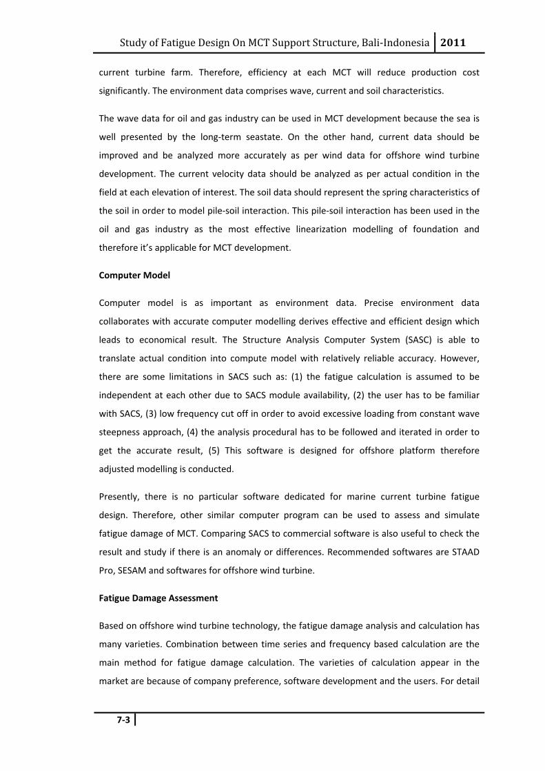
Study of Fatigue Design On MCT Support Structure, Bali‐Indonesia 2011
7‐3
current turbine farm. Therefore, efficiency at each MCT will reduce production cost
significantly. The environment data comprises wave, current and soil characteristics.
The wave data for oil and gas industry can be used in MCT development because the sea is
well presented by the long‐term seastate. On the other hand, current data should be
improved and be analyzed more accurately as per wind data for offshore wind turbine
development. The current velocity data should be analyzed as per actual condition in the
field at each elevation of interest. The soil data should represent the spring characteristics of
the soil in order to model pile‐soil interaction. This pile‐soil interaction has been used in the
oil and gas industry as the most effective linearization modelling of foundation and
therefore it’s applicable for MCT development.
Computer Model
Computer model is as important as environment data. Precise environment data
collaborates with accurate computer modelling derives effective and efficient design which
leads to economical result. The Structure Analysis Computer System (SASC) is able to
translate actual condition into compute model with relatively reliable accuracy. However,
there are some limitations in SACS such as: (1) the fatigue calculation is assumed to be
independent at each other due to SACS module availability, (2) the user has to be familiar
with SACS, (3) low frequency cut off in order to avoid excessive loading from constant wave
steepness approach, (4) the analysis procedural has to be followed and iterated in order to
get the accurate result, (5) This software is designed for offshore platform therefore
adjusted modelling is conducted.
Presently, there is no particular software dedicated for marine current turbine fatigue
design. Therefore, other similar computer program can be used to assess and simulate
fatigue damage of MCT. Comparing SACS to commercial software is also useful to check the
result and study if there is an anomaly or differences. Recommended softwares are STAAD
Pro, SESAM and softwares for offshore wind turbine.
Fatigue Damage Assessment
Based on offshore wind turbine technology, the fatigue damage analysis and calculation has
many varieties. Combination between time series and frequency based calculation are the
main method for fatigue damage calculation. The varieties of calculation appear in the
market are because of company preference, software development and the users. For detail
Study of Fatigue Design On MCT Support Structure, Bali‐Indonesia 2011
7‐4
design it is recommended to use time series approach or frequency based to extract the
actual condition for both wave and current loadings. For screening phase, frequency based is
preferred due to time efficiency.
Environment Impact Assessment (EIA) in Bali Strait
Bali is well known as island of god, rich with species especially underwater biota. This beauty
attracts local tourist as well as international tourist and becomes Indonesia’s top destination
with tremendous revenue per year. As we try to put a new technology in Bali water and
every new technology requires environment impact assessment. Therefore EIA for projects,
construction, transportation, installation, operation and maintenance should be assessed.
For MCT projects, the effect of tidal energy extraction could give negative effect to the
environment and unfortunately, at present, this type of impact is rarely investigated
especially in South East Asia region. Hence, EIA study in Bali strait should be conducted at
the very first time.
Indonesia
One of Indonesia’s major problems is lack of reliable long‐term data. There are more sites
that are applicable for MCT development but many of those have no data or not reliable to
be used. Lack of site measurement is the main problem. However, this problem could be
solved with intensive site measurement starting with potential site such as Capalulu Strait,
Berau Bay and Malacca Strait.
Study of Fatigue Design On MCT Support Structure, Bali‐Indonesia 2011
REFERENCES
REFERENCES
[1] Ainsworth, D. & Thake, J., 2006. Final report on preliminary works associated with 1 MW
tidal turbine. DTI Technology Programme: New and Renewable Energy.
[2] Bahaj, A. & Myers, L., 2003. Fundamentals Applicable to the Utilisation of Marine
Current Turbines for Energy Production. Renewable Energy, 28, pp.2205‐11.
[3] Bahaj, A. & Myers, L., 2004. Analytical Estimates of Energy Yield Potential from the
Alderney Race (Channel Islands) using Marine Current Energy Converters. Renewable
Energy, 29, pp.1931‐45.
[4] Barltrop, N.D.P. & Adams, A.J., 1991. Dynamics of Fixed Marine Structures, Butterworth‐
Heinemann Ltd, Oxford, (1991). ISBN 0‐7506‐1046‐8.
[5] Batten, W., Bahaj, A., Molland, A. & Chaplin, J., 2006. Hydrodynamics of Marine Current
Turbines. Renewable Energy, 31, pp.249‐56.
[6] Black & Veatch, 2005. Phase II UK Tidal Stream Energy Resource Assessment. London:
The Carbon Trust.
[7] Black & Veatch, 2005. Tidal Stream Energy Resource and Technology Summary Report.
Middlesex: The Carbon Trust.
[8] Blunden, L. & Bahaj, A., 2006. Initial Evolution of Tidal Stream Energy Resources at
Portland Bill, UK. Renewable Energy, 31, pp.121‐32.
[9] Blunden, L. & Bahaj, A., 2007. Tidal Energy Resource Assessment for Tidal Stream
Generators. In IMechE Vol.221 Part A: Power and Energy.
[10] Burton, T., Sharpe, D., Jenkins, N. & Bossangi, E., 2001. Wind Energy Handbook. New
York: Wiley.
[11] Charlier, R.H., 1982. Tidal Energy. New York: Van Norstrand Reinhold Company Inc.
[12] Corten, G.P., 2001. Flow Separation on Wind Turbine Blades, PhD Thesis, Utrecht
University. ISBN 90‐393‐2582‐0.
[13] da Rosa, A.V., 2005. Fundamentals of Renewable Energy Processes. London: Elsevier
Academic Press.
[14] Energy Systems Research Unit's of The University of Strathclyde in Glasgow, 2006.
Marine Current Resource and Technology Methodology. [Online] Available at:
http://www.esru.strath.ac.uk/EandE/Web_sites/05‐
06/marine_renewables/home/welcome.htm. On 1 June 2011.
[15] Environmental Change Institute, 2005. Characteristics of the United Kingdom Tidal
Current Power Resource. The Carbon Trust.
[16] EU Commission, 1996. The exploitation of tidal marine currents.

Study of Fatigue Design On MCT Support Structure, Bali‐Indonesia 2011
REFERENCES
[17] Fraenkel, P., 1999. Tidal currents: a major new source of energy for the millennium.
London: ICG Publishing Ltd.
[18] Fraenkel, P., 2007. Marine current turbines: pioneering the development of marine
kinetic energy converters. In IMechE Vol. 221 Part A: J. Power and Energy., 2007.
[19] Freris, L. & Infield, D., 2008. Renewable Energy in Power Systems. Chichester, West
Sussex: John Wiley & Sons Ltd.
[20] Garrett, C. & Cummins, P., 2005. Generating Power from Tidal Currents in Channels. In R.
Soc. Land A.
[21] Hermawan & Hadi, S.P., 2006. Existing Sustainable (Renewable) Energy System in
Indonesia. In The 2nd Joint International Conference on Sustainable Energy and
Environment. Bangkok, 2006.
[22] Hydro‐Oceanographic Service Indonesian Navy, 2009. Tide Tables of Indonesian
Archipelago. Jakarta: Hydro‐Oceanographic Service Indonesian Navy.
[23] Hydro‐Oceanographic Service Indonesian Navy, 2009. Tide Tables of Indonesian
Archipelago. Jakarta: Hydro‐Oceanographic Service Indonesian Navy.
[24] Indonesia's Centre for Data and Information on Energy and Mineral Resources , 2008.
Indonesia Energy Statistics 2008. Jakarta: Ministry of Energy and Mineral Resources.
[25] Indonesia's Centre for Data and Information on Energy and Mineral Resources, 2006.
Blueprint of Indonesia's Energy Management 2006 ‐ 2010. Jakarta: Ministry of Energy
and Mineral Resources.
[26] Indonesia's Centre for Data and Information on Energy and Mineral Resources, 2008.
Key indicator of Indonesia energy and mineral resources. Jakarta: The Ministry of Energy
and Mineral Resources.
[27] Kaltschmitt, M., Streicher, W. & Wiese, A., 2007. Renewable Energy: Technology,
Economics, and Environment. New York: Springer.
[28] Kühn, M., 2001. Dynamics and Design Optimisation of Offshore Wind Energy Conversion
Systems Institute for Wind Energy, Delft University of Technology. ISBN 90‐76468‐07‐9.
[29] LAPI ITB, 2005. Final report of Metocean Design Criteria for General Kangean Block Area,
29 August 2005.
[30] Maunsell, F. & Metro, P., 2007. Scottish Marine Renewable Strategic Environmental
Assessment (SEA): Environmental Assessment. EIA Report. The Scottish Executive.
[31] Millar, D.L., 2007. Wave and Tidal Power. In F. Armstrong & K. Blundell, eds. Energy.
Beyond Oil. Oxford: Oxford University Press, pp.50‐70.

Study of Fatigue Design On MCT Support Structure, Bali‐Indonesia 2011
REFERENCES
[32] Myers, L.E., 2006. Operational Parameters of Horizontal Axis Marine Current Turbines.
PhD Thesis. Southampton: University of Southampton.
[33] Myers, L. & Bahaj, A., 2005. Simulated Electrical Power Potential Harnessed by Marine
Current Turbine Arrays in the Alderney Race. Renewable Energy, 30, pp.1713‐31.
[34] Pandey, V.K. & Pandey, A.C., 2007. Turbulent Kinetic Energy and Its Dissipation Rate of
the Indonesian Throughflow Region via Lombok and Savu Straits. Journal of India
Geophysic Union, 11(2), pp.117‐22.
[35] Pangastuti, W., 2005. Study of tidal use in Seribu Islands Area. Bsc Final Project.
Bandung: Bandung Institute of Technology.
[36] Petroleum and natural gas industries, ISO 19901‐1, 2005. Specific requirements for
offshore structures Part 1: Metocean design and operating considerations International
Organization for Standardization, Geneva, Switzerland.
[37] Tempel, J. van der & Molenaar, D.P., 2002. Wind Turbine Structural Dynamics: a Review
of the Principles for Modern Power Generation, Onshore and Offshore, Publication,
Wind Engineering, Volume 26, No. 4.
[38] Tempel, J. van der, 2006. Design of Support Structures for Offshore Wind Turbines, PhD
Thesis, Delft University of Technology.
[39] Vugts, J.H., 2000. Considerations on the dynamics of support structures for an OWEC
Section Offshore Technology, Delft University of Technology
[40] Vugts, J.H., 2001. Handbook of Bottom Founded Offshore Structures, Lecture notes,
Delft University of Technology.
[41] Weisstein, E.W., 2011. Fast Fourier Transform.
http://mathworld.wolfram.com/FastFourierTransform.html. On 16 May 2011.
[42] Wilson, E.L., 2002. Three‐Dimensional Static and Dynamic Analysis of Structures: A
Physical Approach with Emphasis on Earthquake Engineering, 3rd Ed.

Study of Fatigue Design On MCT Support Structure, Bali‐Indonesia 2011
APPENDICES
APPENDICES
Appendix A1 Environment Data
Appendix A2 Computer Model Plot
Appendix A3 Output Listing