Study of Load Distribution Measures for High-performance

UNIVERSIDADE FEDERAL DO RIO GRANDE DO SULINSTITUTO DE INFORMÁTICA

PROGRAMA DE PÓS-GRADUAÇÃO EM COMPUTAÇÃO

FLAVIO ALLES RODRIGUES

Study of Load Distribution Measures forHigh-performance Applications

Thesis presented in partial fulfillmentof the requirements for the degree ofMaster of Computer Science

Advisor: Prof. Dr. Lucas Mello Schnorr

Porto AlegreOctober 10, 2016

CIP — CATALOGING-IN-PUBLICATION

Alles Rodrigues, Flavio

Study of Load Distribution Measures for High-performance Applications / Flavio Alles Rodrigues. –Porto Alegre: PPGC da UFRGS,

.

86 f.: il.

Thesis (Master) – Universidade Federal do Rio Grandedo Sul. Programa de Pós-Graduação em Computação,Porto Alegre, BR–RS,

. Advisor: Lucas Mello Schnorr.

1. High-performance computing. 2. Parallel computing.3. Performance analysis. 4. Load balance. I. Mello Schnorr,Lucas. II. Título.

UNIVERSIDADE FEDERAL DO RIO GRANDE DO SULReitor: Prof. Carlos Alexandre NettoVice-Reitor: Prof. Rui Vicente OppermannPró-Reitor de Pós-Graduação: Prof. Vladimir Pinheiro do NascimentoDiretor do Instituto de Informática: Prof. Luis da Cunha LambCoordenador do PPGC: Prof. Luigi CarroBibliotecária-chefe do Instituto de Informática: Beatriz Regina Bastos Haro

ACKNOWLEDGEMENTS

I’d like to thank Lucas for the opportunity he gave me and, most impor-

tantly, the guidance throughout this process.

I thank my brother for being the exemplary older sibling. Your success

drives me to try harder, to be better. I thank my father for the example of per-

severance, from which I draw the will to move forward. I thank my mother for

dedicating her to life to her children, for giving everything she has to us. Without

them none of this would be even remotely possible.

Last, but certainly not least, I thank Flavia for all the support, the advice,

and patience. I would not be here, writing these acknowledgments, if it wasn’t

for you.

ABSTRACT

Load balance is essential for parallel applications to perform at their highest pos-

sible levels. As parallel systems grow, the cost of poor load distribution increases

in tandem. However, the dynamic behavior the distribution of load possesses

in certain applications can induce disparities in computational loads among re-

sources. Therefore, the process of repeatedly redistributing load as execution pro-

gresses is critical to achieve the performance necessary to compute large scale

problems with such characteristics. Metrics quantifying the load distribution are

an important facet of this procedure. For these reasons, measures commonly used

as load distribution indicators in HPC applications are investigated in this study.

Considering the dynamic and recurrent aspect in load balancing, the investiga-

tion examines how these metrics quantify load distribution at regular intervals

during a parallel application execution. Six metrics are evaluated: percent imbal-

ance, imbalance percentage, imbalance time, standard deviation, skewness, and kurtosis.

The analysis reveals the virtues and deficiencies each metric has, as well as the

differences they register as descriptors of load distribution progress in parallel

applications. As far as we know, an investigation as the one performed in this

work is unprecedented.

Keywords: High-performance computing. parallel computing. performance

analysis. load balance.

Estudos de Medidas de Distribuição de Carga

para Aplicações de Alto Desempenho

RESUMO

Balanceamento de carga é essencial para que aplicações paralelas tenham desem-

penho adequado. Conforme sistemas de computação paralelos crescem, o custo

de uma má distribuição de carga também aumenta. Porém, o comportamento

dinâmico que a carga computacional possui em certas aplicações pode induzir

disparidades na carga atribuída a cada recurso. Portanto, o repetitivo processo de

redistribuição de carga realizado durante a execução é crucial para que problemas

de grande escala que possuam tais características possam ser resolvidos. Medi-

das que quantifiquem a distribuição de carga são um importante aspecto desse

procedimento. Por estas razões, métricas frequentemente utilizadas como indi-

cadores da distribuição de carga em aplicações paralelas são investigadas nesse

estudo. Dado que balanceamento de carga é um processo dinâmico e recorrente,

a investigação examina como tais métricas quantificam a distribuição de carga

em intervalos regulares durante a execução da aplicação paralela. Seis métricas

são avaliadas: percent imbalance, imbalance percentage, imbalance time, standard de-

viation, skewness e kurtosis. A análise revela virtudes e deficiências que estas me-

didas possuem, bem como as diferenças entres as mesmas como descritores da

distribuição de carga em aplicações paralelas. Uma investigação como esta não

tem precedentes na literatura especializada.

Palavras-chave: Computação de alto desempenho, computação paralela, análise

de desempenho, balanceamento de carga.

LIST OF ABBREVIATIONS AND ACRONYMS

AMR Adaptive Mesh Refinement

CPP Call Path Profiles

CCT Calling Context Tree

CSV Comma-separated Values

HPC High-performance Computing

SPMD Single Program, Multiple Data

VM Virtual Machine

LIST OF SYMBOLS

σ Standard Deviation

γ1 Skewness

γ2 Kurtosis

λ Percent Imbalance

I% Imbalance Percentage

It Imbalance Time

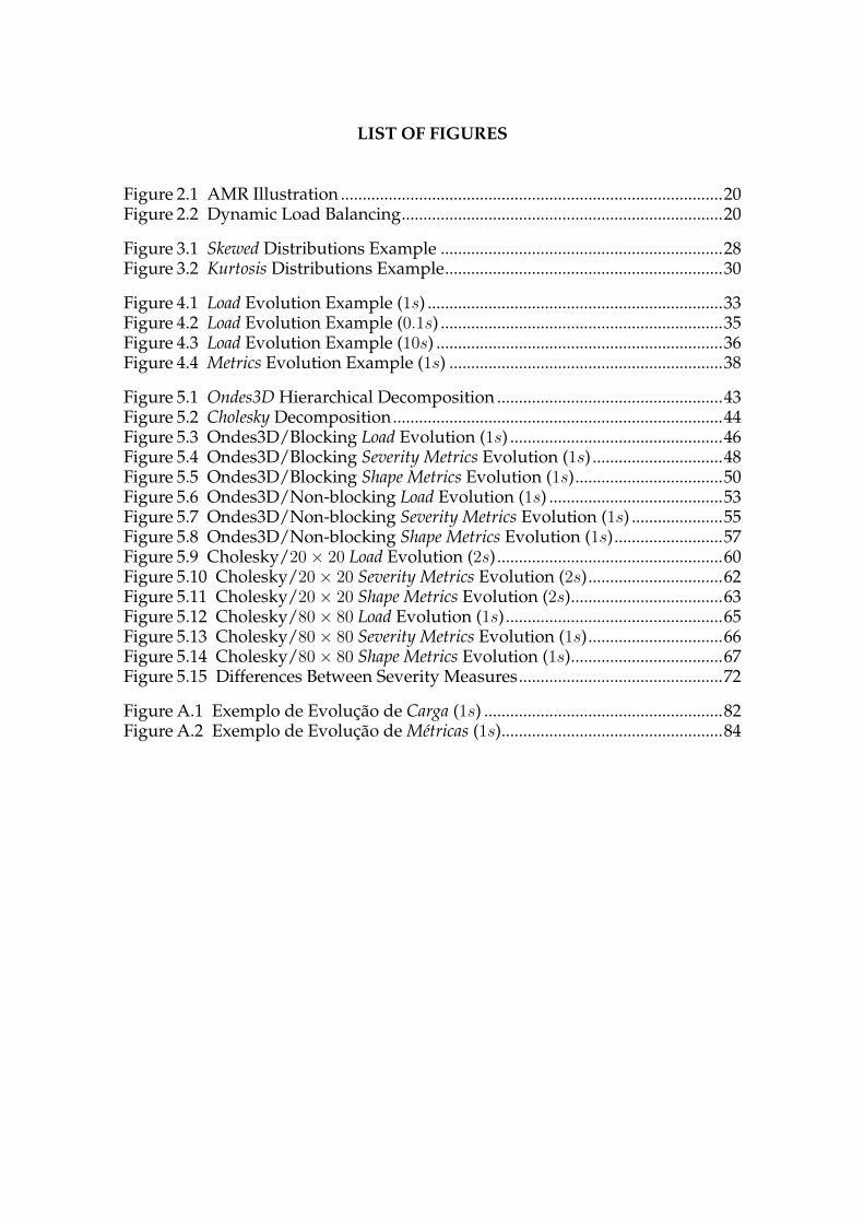
LIST OF FIGURES

Figure 2.1 AMR Illustration ........................................................................................20Figure 2.2 Dynamic Load Balancing..........................................................................20

Figure 3.1 Skewed Distributions Example .................................................................28Figure 3.2 Kurtosis Distributions Example................................................................30

Figure 4.1 Load Evolution Example (1s) ....................................................................33Figure 4.2 Load Evolution Example (0.1s) .................................................................35Figure 4.3 Load Evolution Example (10s) ..................................................................36Figure 4.4 Metrics Evolution Example (1s) ...............................................................38

Figure 5.1 Ondes3D Hierarchical Decomposition ....................................................43Figure 5.2 Cholesky Decomposition............................................................................44Figure 5.3 Ondes3D/Blocking Load Evolution (1s) .................................................46Figure 5.4 Ondes3D/Blocking Severity Metrics Evolution (1s) ..............................48Figure 5.5 Ondes3D/Blocking Shape Metrics Evolution (1s)..................................50Figure 5.6 Ondes3D/Non-blocking Load Evolution (1s) ........................................53Figure 5.7 Ondes3D/Non-blocking Severity Metrics Evolution (1s) .....................55Figure 5.8 Ondes3D/Non-blocking Shape Metrics Evolution (1s).........................57Figure 5.9 Cholesky/20× 20 Load Evolution (2s)....................................................60Figure 5.10 Cholesky/20× 20 Severity Metrics Evolution (2s)...............................62Figure 5.11 Cholesky/20× 20 Shape Metrics Evolution (2s)...................................63Figure 5.12 Cholesky/80× 80 Load Evolution (1s)..................................................65Figure 5.13 Cholesky/80× 80 Severity Metrics Evolution (1s)...............................66Figure 5.14 Cholesky/80× 80 Shape Metrics Evolution (1s)...................................67Figure 5.15 Differences Between Severity Measures...............................................72

Figure A.1 Exemplo de Evolução de Carga (1s) .......................................................82Figure A.2 Exemplo de Evolução de Métricas (1s)...................................................84

LIST OF TABLES

Table 5.1 Turing Experimental Platform Configuration..........................................42

CONTENTS

1 INTRODUCTION.....................................................................................................112 BACKGROUND AND MOTIVATION................................................................132.1 Scientific, High-performance, and Parallel Computing ................................132.2 Parallel Programming ..........................................................................................142.2.1 Decomposition.....................................................................................................152.2.2 Mapping ...............................................................................................................172.3 Load Balance ..........................................................................................................182.4 Motivation ..............................................................................................................213 RELATED WORK .....................................................................................................234 METHODOLOGY ....................................................................................................324.1 Load Analysis ........................................................................................................324.2 Metrics Analysis....................................................................................................364.3 Data & Tools...........................................................................................................395 EXPERIMENTAL RESULTS AND ANALYSIS...................................................415.1 Experimental Setup: Platform Configuration and Case Studies .................415.1.1 Experimental Platform .......................................................................................415.1.2 Case Study: Ondes3D.........................................................................................425.1.3 Case Study: Cholesky Decomposition.............................................................435.2 Metrics Analysis....................................................................................................455.2.1 Ondes3D...............................................................................................................465.2.2 Cholesky...............................................................................................................595.3 Summary.................................................................................................................706 CONCLUSION..........................................................................................................74REFERENCES ...............................................................................................................76APPENDIX A — ESTUDOS DE MEDIDAS DE DISTRIBUIÇÃO DE CARGA

PARA APLICAÇÕES DE ALTO DESEMPENHO......................................79A.1 Introdução .............................................................................................................79A.2 Metodologia ..........................................................................................................80A.2.1 Análise de Carga ................................................................................................81A.2.2 Análise das Métricas..........................................................................................82A.3 Dados e Ferramentas ...........................................................................................84A.4 Resultados e Trabalhos Futuros ........................................................................85

11

1 INTRODUCTION

High-performance computing (HPC) consists in employing parallel process-

ing concepts to execute applications that would, otherwise, either consume an

enormous amount of time when computed in a sequential setting or would not

be computable at all. In other words, HPC denotes the idea of accumulating

processing power so as to deliver performance that would be unachievable in a

single commodity desktop or mobile computer. Hence, HPC allows for complex

computational problems that possess massive memory, processing, and network

bandwidth requirements to be computed in acceptable time. Users of HPC sys-

tems are predominantly scientists of diverse fields (DROR et al., 2012) (MICHA-

LAKES; VACHHARAJANI, 2008). However, engineers (ELIAS; COUTINHO,

2007) and economists (PAGÈS; WILBERTZ, 2012) make use of high-performance

computing methods and systems as well.

HPC and parallel computing are, thus, correlated, with the latter being

applied to achieve the former’s goals. Load balance is essential for parallel ap-

plications to perform at their highest possible levels. As parallel systems grow,

the cost of poor load distribution increases in tandem (BONETI et al., 2008). A

proper load balance is even more important for large scale applications.

However, in a class of applications referred to as irregular, the dynamic

behavior load possesses can induce disparities in computational loads among

resources. Therefore, the process of repeatedly redistributing computational load

between resources as execution progresses is critical to achieve the performance

necessary to compute large scale problems. Since high-performance applications

are increasingly irregular (FEO et al., 2011), dynamic load balancing is of vital

importance in high-performance computing today.

Load balancing involves measuring the state of load distribution, deciding

on how to redistribute work, and actually performing the reassignment of load.

Therefore, metrics quantifying the load distribution are an important facet of this

procedure. The process of rebalancing computation load between resources in-

volves an overhead that might impact performance negatively if performed un-

necessarily. Additionally, delaying load reassignment might also affect appli-

cation performance. Considering the centrality of adequate load balance, these

measures must be completely understood to be interpreted correctly and guide

12

load balancing effectively.

As a result, metrics commonly used as load distribution indicators in HPC

applications are examined in this study. Considering the dynamic and recurrent

aspect in load balancing, the investigation examines how these metrics quantify

load distribution at regular intervals during a parallel application execution, in-

stead of simply considering an aggregate including the complete computation.

In other words, as load distribution evolves, the measures are computed to deter-

mine how they communicate this progress.

Six metrics are evaluated: percent imbalance, imbalance percentage, imbalance

time, standard deviation, skewness, and kurtosis. The analysis is expected to reveal

the virtues and deficiencies each metric has, as well as the differences they regis-

ter as descriptors of load distribution progress along time in parallel applications.

As far as we know, an investigation as the one proposed here has never been per-

formed before.

The methodology employed in the study relies on visual comparative anal-

ysis of depictions of both the load distribution progress and the reports load

metrics provide concerning this progress. Several parallel application executions

were used to perform the study, providing a comprehensive set of load distribu-

tion patterns. Execution traces are used to gather information on parallel appli-

cation executions.

The rest of this document is structured as follows. Chapter 2 discusses

concepts that are important for the full comprehension of this dissertation, as

well as the motivation behind this study. Chapter 3 provides a literature review in

load imbalance measurement. Afterwards, the methodology through which the

evaluation proposed in this dissertation is performed is presented in Chapter 4.

Experimental results and analysis are located in Chapter 5. Chapter 6 contains

the concluding remarks and provides directions for future work.

13

2 BACKGROUND AND MOTIVATION

This chapter presents concepts that are indispensable to the proper under-

standing of the problem that is dealt with in this document. The chapter starts

with a brief discussion on scientific, high-performance, and parallel computing

that establishes how these concepts are related and, also, the importance they

have in science at the present time (Section 2.1).

A section devoted to explaining what constitutes the fundamental aspects

of parallel programming follows (Section 2.2). Computational load, load imbal-

ance and load distribution measures are explored afterwards (Section 2.3). The

closing section of the chapter provides both the motivation behind the research

presented in this document, as well as the proposal put forward in it (Section 2.4).

2.1 Scientific, High-performance, and Parallel Computing

The term scientific computing denotes a perspective of science where the

creation of knowledge or the simple understanding of a particular subject are

achieved through the use of computational resources and techniques. More specif-

ically, computational science, another term by which scientific computing is known,

pursuits to decipher scientific phenomena through the use and analysis of math-

ematical models on high-end computers. As a consequence, computing is today

perceived as an indispensable tool for the evolution of scientific knowledge, along

with the classic methods of theoretical analysis and experimental observations

(HEY; TANSLEY; TOLLE, 2009). In 2005, the United States Presidential Information

Technology Advisory Committee corroborated this assessment by publishing a re-

port asserting that computational science constituted a third pillar of scientific re-

search (REED et al., 2005). Numerical simulations performed on computers with

enormous processing power, for instance, allow research into complex natural

systems that would otherwise be unfeasible through experimental observations,

due to either financial constraints or time limitations.

High-performance computing, an inherent component of scientific computing,

consists in using machines that far exceed commodity systems computing power

in order to solve complex computational problems. High-performance computer

designs target the maximum computer power to solve a single large problem in

14

the shortest amount of time. In contrast, the usual architectural goal of com-

modity computers is to solve a small number of somewhat large problems or

even a large number of small problems. HPC enables scientists to solve com-

plex problems by running applications that require high network bandwidth,

large memory capacity, and very high computing capabilities within a reasonable

amount of time. HPC is applied in the modeling of phenomena in fields as di-

verse as computational finance (PAGÈS; WILBERTZ, 2012) (FATICA; PHILLIPS,

2013), molecular biology (DROR et al., 2012) (LIGOWSKI; RUDNICKI, 2009),

and climate modeling (MICHALAKES; VACHHARAJANI, 2008) (QUIRINO;

DELGADO; ZHANG, 2014).

Parallel computing is a form of computation in which multiple calculations

are performed simultaneously. This strategy is premised on the assumptions that,

first, a problem can often be split into smaller problems and, second, that these

smaller problems can be computed concurrently. As a consequence, parallel com-

putations are executed in more than one processing element. These processing el-

ements could be located within a single computer that possesses multiple proces-

sors, several networked computers, some form of specialized hardware or a com-

bination of these options. The main objective of parallel computing is to provide

answers to large problems in less time than in traditional sequential computing

by exploiting the power of parallel systems. For this reason, parallel computation

is intrinsic to the field of high-performance computing.

2.2 Parallel Programming

Sequential programming consists in defining an ordering of operations

that ought to be followed in order for a computation to succeed. Parallel pro-

gramming, on the other hand, involves not only defining the sequence of steps

that must be performed as well as determining which of these steps can be ex-

ecuted simultaneously. Dividing a computation into smaller parts and assign-

ing those parts to different computational resources are central tasks in parallel

programming. Those procedures are referred to as decomposition and mapping, re-

spectively. While the former determines the potential degree of concurrency the

computation has, the latter controls how much of that concurrency is achieved.

The remainder of this section is devoted to discussing decomposition (Subsection

15

2.2.1) and mapping (Subsection 2.2.2). Basic definitions and related concepts are

presented, along with the most common techniques parallel programmers em-

ploy to perform these operations.

2.2.1 Decomposition

Decomposition is the process of partitioning a computation into smaller

units of work that can be performed concurrently. The units of computation that

the problem is divided into are commonly called tasks. Decomposing a compu-

tation into smaller parts induces the emergence of dependence relations among

tasks. A task, for instance, might depend on the completion of other tasks in

order to begin execution (e.g. task C input might be tasks A and B output).

Granularity is a concept related to the process of decomposing a compu-

tation. In a broad sense, it can be defined as the degree to which a material is

constituted of separate, discernible parts. In the specific context of parallel com-

puting, granularity refers to the amount and size of the tasks a computation is

divided into. A computation that has been split into a small amount of large

tasks is referred to as coarse-grained. Conversely, a computation decomposed into

a large amount of small tasks is referred to as fine-grained. The qualifiers large and

small are meant to quantify the size of tasks in both code size and execution time.

The finer the granularity, the greater the number of tasks the computation

is divided into and, consequently, the greater the potential for parallelism. The

greater parallelism resulting from increased granularity is said to be potential,

and not guaranteed, because more tasks usually lead to more overhead in both

scheduling and communication. Therefore, in order to achieve optimal perfor-

mance in any decomposing process, there is a balance to be found between the

granularity level and the overhead produced by increased parallelism.

Multiple techniques exist to guide the decomposition process. The most

common are recursive, data, exploratory, and speculative (GRAMA et al., 2003).

Recursive and data decomposition techniques can be employed to decompose a

wide range of problems. Speculative and exploratory techniques, on the other

hand, are applied only in specific classes of problems. Each of these approaches

is further discussed next.

16

2.2.1.1 Recursive

Recursive decomposition is based on the computational concept of recursion.

Recursion is a computing technique where smaller, simpler, solutions for a prob-

lem are the base upon which the solution to the overall problem is built. More

specifically, a recursion has one or more recursive cases for which it recurs, fur-

ther splitting the problem. Additionally, a recursion has one or more base cases

for which it produces results directly, without recurring. The base cases are re-

ferred to as terminating cases, since they end the chain of recursion.

A recursive algorithm, hence, operates by repeatedly splitting a problem

into sub-problems until the sub-problems are simple enough to be computed di-

rectly. This computational strategy results in natural concurrency, as the different

sub-problems into which the computation is split are independent and, therefore,

can be solved simultaneously. The recursive decomposition technique consists

merely in designing the problem solution for which one wants to compute in

parallel as a recursive computation.

2.2.1.2 Data

In algorithms that operate on large data structures, the technique known

as data decomposition is appropriate to induce parallelism. The computation is de-

composed into tasks by partitioning the data upon which computations will be

performed and using this partitioning to generate the decomposition of the com-

putation into tasks. Frequently in data-based decompositions all tasks perform

the same operations on their respective data partition. Data partitioning can be

performed in several different ways.

Partitioning Input Data. In computations where elements of the input are

used independently to compute the output, it is possible to partition the input

data, and then use this partitioning to derive task concurrency. In this scenario, a

task is created for each partition of the input data.

Partitioning Output Data. In computations where elements of the output

can be computed independently, a partitioning of the output data directly induces

a decomposition of the problem into tasks. In such a decomposition scheme,

every task is allocated a fragment of the output to compute.

Other options to induce concurrency through data decomposition include

17

partitioning, when possible, both input and output data. In addition, in compu-

tations that are designed as series of processing stages, data decomposition can

be performed by partitioning the intermediate data between two stages.

2.2.1.3 Exploratory

Many computational problems have their solutions computed by means

of a search in an input space. This class of problems is naturally parallelized

through a decomposition technique known as exploratory decomposition. In this

technique, the space searched for a solution is divided into smaller fragments.

Each fragment is then assigned to a task and explored concurrently. All tasks are

terminated when a solution is found.

2.2.1.4 Speculative

The decomposition technique known as speculative decomposition is appro-

priate in situations where many possibilities of follow-through computation exist

based the output of a preceding computation. In this scenario, while one task

computes the output upon which a decision of what computation will follow,

other tasks – ideally as many as there are computing possibilities following –

concurrently work on the computations of the following stage. When the output

upon which a decision is made is available, the computation corresponding to

the correct option is used while the others are either terminated if they are yet to

finish execution or, otherwise, their output is discarded.

2.2.2 Mapping

As stated earlier, mapping is the procedure in which tasks are delegated

to computational resources for execution. The goal of any mapping process is

to decrease the computation’s execution span. Achieving such result involves

minimizing the overheads associated with concurrent execution of tasks. Inter-

resource communication and resource idleness are the most fundamental forms

of overhead in parallel computing (GRAMA et al., 2003).

Consequently, the process of assigning tasks onto resources has two con-

crete objectives: reducing the amount of time resources are idle while others

18

compute and minimizing interactions between different resources. The first is

achieved by maximizing concurrency through the simultaneous assignment of

tasks that do not possess dependencies among them onto different resources. The

second is handled through the allocation of tasks which communicate substan-

tially into the same resources.

Devising an optimal schedule associating tasks, time, and resources is con-

sidered to be NP-complete (ULLMAN, 1975). The class of NP-complete problems

is composed by computational problems that are regarded as being intractable

and, thus, beyond of what is feasible computationally (TAYLOR, 1998).

Since finding an optimal mapping is unattainable, numerous heuristics

have been developed to find acceptable solutions to this problem. These heuris-

tics can be performed either statically or dynamically. In static mapping, tasks are

allocated to resources before execution starts. In dynamic mapping, the allocation

of work to resources is conducted during the execution of the program.

2.3 Load Balance

The concept of computational load denotes work that is essential to accom-

plish an application’s goals. A proper definition of what precisely work means is

easier to achieve by providing a negative definition or, in other words, by stating

what the concept is not. Work refers to any operation that is not a form of commu-

nication, interaction, or synchronization. Hence, overhead operations that exist

as a consequence of parallelizing a computation are not considered load. Com-

putational load is commonly measured in units of time, although it can be quan-

tified by resource utilization as well (ARZUAGA; KAELI, 2010) (XU; HUANG;

BHUYAN, 2004).

The discussion in the previous section stated that one of mapping’s main

goals is to avoid resource idleness. The most natural strategy to achieve that goal

is to divide the application’s computational load equally - if the resources are ho-

mogeneous in terms of their computing power - or according to their capabilities

- in the case where the resources are heterogeneous with regards to their com-

puting power. In other words, in order to accomplish the best performance, the

mapping of tasks in a parallel application execution ought to attain load balance

among resources.

19

Load imbalance, thus, occurs when computational load distribution is un-

equal between the resources that constitute a parallel system. As the number

of resources in a parallel machines grows, the performance penalty inflicted by

load imbalance increases as well (BONETI et al., 2008). Today’s most powerful

machines contain hundreds of thousands of processors. And in the future, super-

computers will display even more parallelism. Hence, in this scenario, balanced

load distribution is critical to obtain adequate performance in parallel codes.

In a number of parallel applications, static mapping strategies are capable

of providing proper load balance within resources. For a certain class of paral-

lel applications, however, redistributing computational load among resources as

execution progresses is crucial for achieving acceptable performance. The appli-

cations that constitute this class are known as irregular applications. A parallel

application is irregular if it presents at least one of three possible characteristics:

irregular control structures (e.g. conditional statements), irregular data structures

(e.g. trees, graphs), or irregularity in interaction patterns (YELICK, 1993).

Irregular applications are commonplace nowadays. In the past 10 years,

a new generation of HPC applications that operate on large, irregular, data sets

has emerged. Bioinformatics, social networks, natural language processing, and

pattern recognition are all examples of irregular applications that deal with im-

portant, relevant topics of research today (FEO et al., 2011).

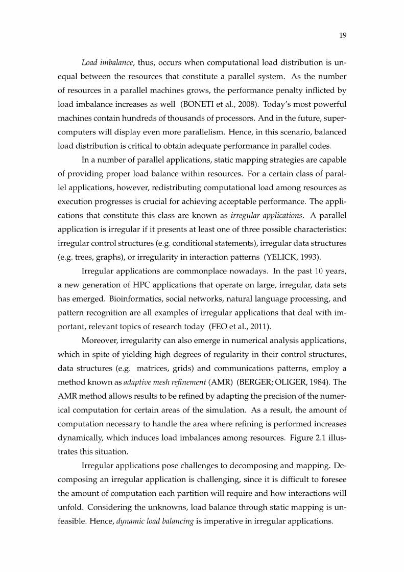
Moreover, irregularity can also emerge in numerical analysis applications,

which in spite of yielding high degrees of regularity in their control structures,

data structures (e.g. matrices, grids) and communications patterns, employ a

method known as adaptive mesh refinement (AMR) (BERGER; OLIGER, 1984). The

AMR method allows results to be refined by adapting the precision of the numer-

ical computation for certain areas of the simulation. As a result, the amount of

computation necessary to handle the area where refining is performed increases

dynamically, which induces load imbalances among resources. Figure 2.1 illus-

trates this situation.

Irregular applications pose challenges to decomposing and mapping. De-

composing an irregular application is challenging, since it is difficult to foresee

the amount of computation each partition will require and how interactions will

unfold. Considering the unknowns, load balance through static mapping is un-

feasible. Hence, dynamic load balancing is imperative in irregular applications.

20

Figure 2.1: Adaptive Mesh Refinement Illustration

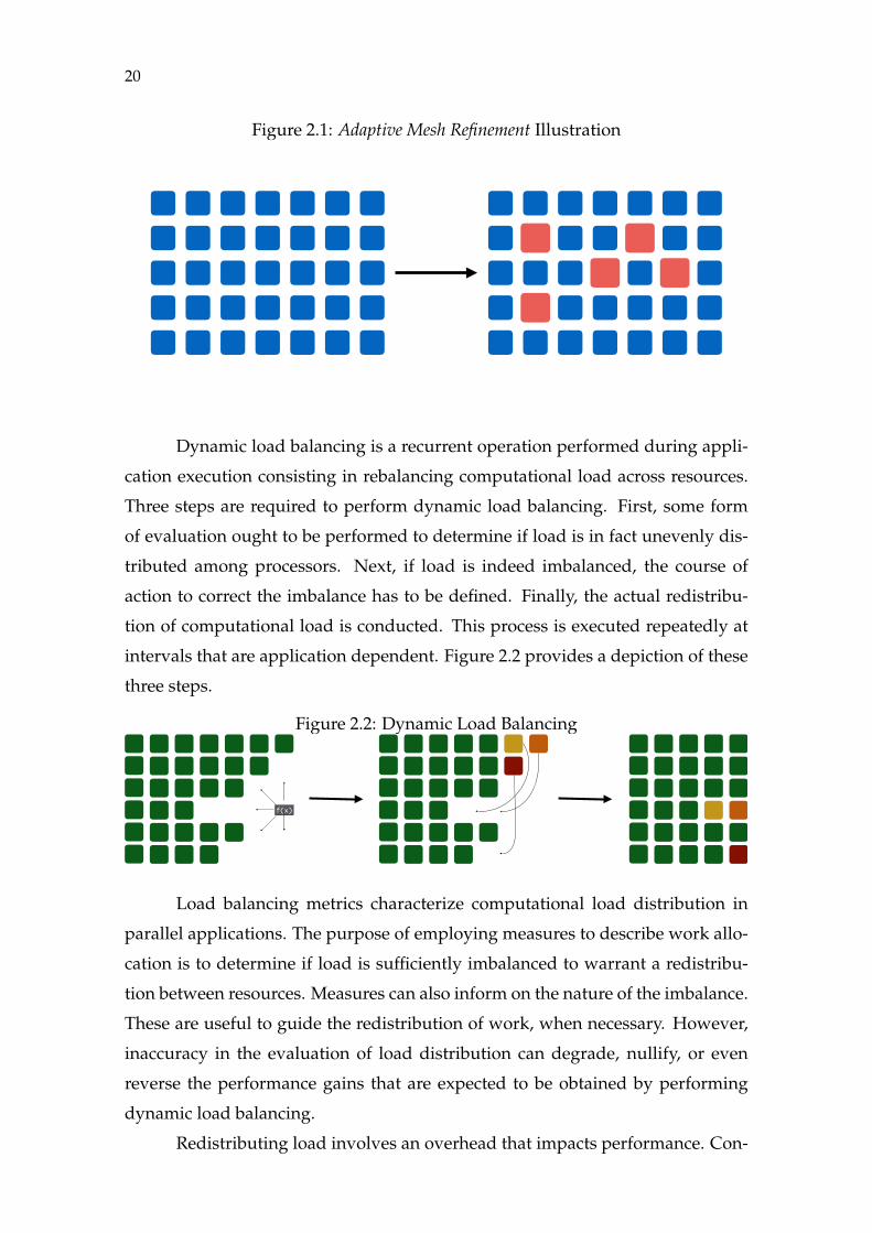
Dynamic load balancing is a recurrent operation performed during appli-

cation execution consisting in rebalancing computational load across resources.

Three steps are required to perform dynamic load balancing. First, some form

of evaluation ought to be performed to determine if load is in fact unevenly dis-

tributed among processors. Next, if load is indeed imbalanced, the course of

action to correct the imbalance has to be defined. Finally, the actual redistribu-

tion of computational load is conducted. This process is executed repeatedly at

intervals that are application dependent. Figure 2.2 provides a depiction of these

three steps.

Figure 2.2: Dynamic Load Balancing

f(x)

Load balancing metrics characterize computational load distribution in

parallel applications. The purpose of employing measures to describe work allo-

cation is to determine if load is sufficiently imbalanced to warrant a redistribu-

tion between resources. Measures can also inform on the nature of the imbalance.

These are useful to guide the redistribution of work, when necessary. However,

inaccuracy in the evaluation of load distribution can degrade, nullify, or even

reverse the performance gains that are expected to be obtained by performing

dynamic load balancing.

Redistributing load involves an overhead that impacts performance. Con-

21

sequently, in the case where load redistribution is conducted without need, the

application’s performance will be negatively affected. Additionally, not perform-

ing load rebalancing when necessary and, thus, keeping load imbalanced has an

impact in the application’s performance. Therefore, any metric employed as a

descriptor of load distribution in a load balancing process is required to be accu-

rate. On the case that the measure used as the guide as to whether or not initiate

load redistribution is not reliable, the whole procedure of load balancing might

become more harmful than beneficial.

2.4 Motivation

Hence, given the rise of irregular applications and the trend of increasing

processor counts in parallel systems, load balancing is an essential part of HPC

at the present moment. As described above, the first phase in the process of load

redistribution involves evaluating the current state of work allocation. The eval-

uation consists in computing some form of measure (or measures) that quantifies

some aspect of load distribution.

Several different metrics are employed as load imbalance indicators. The

process of load redistribution involves continually monitoring the status of load

imbalance across resources. A measure characterizing load unevenness is re-

quired to perform such monitoring. Moreover, some metrics are employed to

inform not on the degree of differences in computational loads, but on providing

information on the nature of these differences. Hence, in the event of load re-

distribution being deemed as necessary by a metric that computes the disparities

in load distribution, this latter group of measures provides information useful in

the process of load reassignment.

Given the importance of proper load distribution, metrics employed as

guides in this process must be understood in their peculiarities to be properly

used. For large scale applications, the performance penalties of incurring in the

error of unnecessarily redistributing load or, even worst, of not performing load

balancing when needed are high.

For these reasons, this study aims to assess metrics commonly employed

as load distribution descriptors in load balancing heuristics applied in HPC ap-

plications. Given the dynamic and repetitive characteristics in the process of load

22

redistribution, measures will be examined in how they quantify load as execution

advances. In other words, computational load across resources will be examined

at fixed, regular, intervals rather than as a single aggregate that encompasses the

complete execution. Additionally, the evaluation will consider only measures

that are suited to homogeneous multiprocessing environments.

The measures chosen to be part of the analysis can be divided in two

groups. Percent imbalance, imbalance percentage, imbalance time, and standard de-

viation are metrics that provide a quantification of how uneven work distribution

is. These measures inform load balancers on the severity of imbalance and, con-

sequently, their usage is appropriate to determine when to perform work redis-

tribution. The second group, constituted by skewness and kurtosis, quantify load

distribution characteristics such as its symmetry and its source of dispersion and,

as a result, provide knowledge on the most suitable means of rebalancing load.

In summary, the analysis of the different measures selected as part of this

study aims to evaluate the behavior of the metrics as indicators of load distri-

bution evolution in parallel applications. Both the strengths and the deficiencies

each measure has are anticipated to be revealed. Additionally, the investigation

should inevitably uncover the differences in the measures descriptions of load

distribution progress. As far as we know, an investigation of this nature does not

exist in the scientific literature.

The following chapter provides a review on the state of art concerning

the measurement of load imbalance. The reasoning behind the selection of the

aforementioned measures as targets of the study proposed in this document will

be explained as well. Additionally, these six load distribution metrics will be

properly explored.

23

3 RELATED WORK

Several load distribution metrics exist in the literature. One of the most

commonly used is the percent imbalance metric (PEARCE et al., 2012). Two other

metrics of load imbalance, which as percent imbalance impart a sense of the load

distribution disparities, are imbalance percentage and imbalance time (DEROSE;

HOMER; JOHNSON, 2007).

Statistical moments, such as standard deviation, skewness, and kurtosis are

able to assess several aspects of load allocation, like the magnitude of the disper-

sion of computational loads and whether the dispersion is a product of a few out-

liers or multiple modestly imbalanced resources. For these reasons, those mea-

sures can be employed to gauge load distribution (PEARCE et al., 2012) (XU;

HUANG; BHUYAN, 2004) (ARZUAGA; KAELI, 2010).

Call path profiles (CPP) are also used for the identification of load imbalance

in parallel applications (TALLENT; ADHIANTO; MELLOR-CRUMMEY, 2010).

A call path profile is represented by a calling context tree (CCT). The root of the

tree is the entry point of the program and the leaves are samples collected during

program execution. Hence, the path from the root to a leaf’s parent represents

the sample’s calling context. There is exactly one CCT per process/thread.

The analysis of load imbalance through call path profiles consists in per-

forming a post-mortem summarization of the data collected in the multiple CCT’s.

A calling context is regarded as balanced if every instance completes in roughly

the same amount of time. In other words, a node (i.e. call path) will be consid-

ered balanced if all its samples across all threads of execution have computed in

a similar time span.

One issue this analysis presents, given the loss of temporal information as-

sociated with calling contexts imposed by the use of profiling, is that an analysis

devoted to understanding the dynamic aspects of load imbalance is unfeasible.

Hence, by using profiles one cannot reveal load distribution patterns across time,

but only a total aggregate encompassing the whole computation.

The focus on calling contexts is yet another issue of the approach proposed

in the article. Load balancers are interested in determining if resources are bal-

anced with regards to their respective computational loads. In Single Program,

Multiple Data (SPMD) applications, since every resource executes the same op-

24

erations, resource and calling context balance are equivalent. However, this is

not true in other programming paradigms, since CCT’s might differ, one cannot

establish if load is balanced between resources using this methodology.

Virtualized Server Load is a measure that quantifies the load of a virtualized

enterprise server as a function of the virtual machines (VM) operating on the

machine (ARZUAGA; KAELI, 2010). It considers virtual CPU, memory, and disk

utilization information specific to each VM running on the server to determine

its load. The quantification of load imbalance in the set of servers that constitute

the computational environment is derived from the ratio between the standard

deviation of the Virtualized Server Load of all servers and the average Virtualized

Server Load for the same set of machines.

This load metric, however, is oriented towards a specific computational

environment, virtualized enterprise servers. Moreover, part of the originality of

the work is not in the proposal of a load distribution measurement, but in the defi-

nition of a load metric. Load imbalance is measured by using standard statistical

moments. This dissertation, however, is concerned solely in investigating load

distribution measurements.

There are other approaches to gauge load distribution in parallel applica-

tions and environments. The use of critical path profiles as a method to detect load

imbalance has been proposed as well (BOHME et al., 2012). However, the issue

of loss of temporal information observed when the use of call path profiles was

discussed is valid for this mechanism.

Load distribution metrics that consider the possibility of heterogeneity in

the parallel system where the application is executed, as well as the prospect of

the application running on a shared environment, also exist (YANG et al., 2003).

Nevertheless, the study proposed here is concerned solely with HPC applications

running on homogeneous platforms without having to share this environment.

In summary, the study of load imbalance metrics proposed in this disserta-

tion is oriented towards HPC environments, where computational resources are

not subject to virtualization and the applications are not expected to share the

platform with other workloads through the use of another method. Moreover,

the measure must be applicable as a gauge of the dynamic load distribution. In

other words, the distribution of load must be suited to be computed for arbitrary

intervals during the computation, and not only as a total aggregate encompass-

25

ing all of the execution. Finally, the focus is in studying exclusively measures that

are appropriate for homogeneous multiprocessing parallel computing systems.

For these reasons, percent imbalance, imbalance percentage, imbalance time,

standard deviation, skewness, and kurtosis were the metrics chosen to be part of

the study. All are appropriate as dynamic load distribution metrics for homoge-

neous HPC systems. A discussion considering these metrics as measures of load

distribution follows. Each metric is considered separately, in the order in which

they were listed at the beginning of the paragraph. Afterwards, a brief summary

on the metrics similarities and differences is presented.

Percent Imbalance

Percent imbalance (λ) (PEARCE et al., 2012) is a load distribution measure

that characterizes how unevenly work is distributed among resources. The met-

ric considers the current state of load distribution to compute the performance, in

percentage points, that would be gained if loads were properly balanced across

resources. In other words, Percent imbalance is a measure that quantifies the sever-

ity of load imbalance. The mathematical formula used to compute the measure

follows below.

λ = (Lmax

L− 1)× 100 (3.1)

In the equation above, λ represents the measure of interest, percent imbal-

ance). Lmax symbolizes the load of the resource that has the greatest computa-

tional load during the period of time for which the metric is being computed. L

is the average load across all resources for the same period of time. From the

equation, it can be deduced that percent imbalance is a dimensionless quantity.

Imbalance Percentage

Imbalance percentage (I%) (DEROSE; HOMER; JOHNSON, 2007) is a load

distribution metric that, like percent imbalance, gauges how severe load imbal-

ance is. The measure considers the computational loads registered for every re-

source, as well as the number of resources available to quantify load imbalance.

26

Although the measure’s name is similar to the metric described above, its math-

ematical definition is different. Imbalance percentage is derived by computing the

following equation.

I% =Lmax − L

Lmax

× n

n− 1(3.2)

In the formula above, I% stands for imbalance percentage. Lmax represents

the load of the resource that has computed most in the span of time for which the

metric is being calculated for. L is the average load across the resources partici-

pating in the computation for the same span of time. And, finally, n represents

the number of resources. Imbalance percentage is a dimensionless measure.

The interpretation for the imbalance percentage is as follows. The metric

corresponds to the percentage of time that the computing resources, excluding

the most loaded one, are not involved in useful work throughout the period of

time in consideration. Expressed in a different manner, the metric establishes the

percentage of resources’ time available for parallelism that are not used due to

inadequate work distribution.

Imbalance Time

Imbalance time (It) (DEROSE; HOMER; JOHNSON, 2007), using a different

approach than the previous metrics, is yet another measure of load imbalance in

parallel applications. The following formula demonstrates how the measure is

computed.

It = Lmax − L (3.3)

This simple equation establishes that imbalance time (It) for a particular pe-

riod of a computation is given by the subtraction of the highest resource load for

that period (Lmax) by the the average resource load within the same span of time

(L). The measure provides an estimate of the time that would be saved if the load,

for the period of time considered, was perfectly balanced across all resources.

Imbalance time is measured in the same unit as load is quantified. Hence,

if load is measured in seconds, imbalance time will also be quantified in seconds.

Hence, unlike percent imbalance and imbalance percentage which consider load im-

27

balance in terms of percentages of either expected improved performance or of

resources idleness, imbalance time yields a measure in the same dimension as the

one used to quantify load.

Standard Deviation

Standard deviation (σ) is a measure used to quantify the amount of disper-

sion existent in a set of data values. Dispersion denotes a sense of the distance

between the values in a distribution of data points and is contrasted by the dis-

tribution’s central tendency. A measure of statistical dispersion for a particular

distribution of data is a non-negative number that is zero if all the data values are

equal and increases as the data becomes more diverse.

Standard deviation is one of many measures of dispersion for a sample of

data or a probability distribution. Examples of other measures include entropy,

coefficient of variation, and variance - from which the standard deviation is derived

by extracting its square root. However, unlike these other metrics of dispersion,

standard deviation is expressed in the same unit of measure as the data from

which it was calculated. This aspect makes standard deviation’s interpretation rea-

sonably straightforward when compared to the other measures.

The use of standard deviation as a load distribution metric involves comput-

ing its value for the set of loads in every resource participating in the computa-

tion. In the most common situation where computational load is quantified by

the amount of time the resource was engaged in work during a given interval,

standard deviation will be quantified in the same time unit used to gauge load.

High standard deviation, in this context, indicates that loads across resources

are spread far from the average and, thus, work is poorly distributed. On the

other hand, low standard deviation indicates that loads are clustered closely around

the mean and the load can be considered to be properly distributed. Hence, Stan-

dard deviation, as percent imbalance, imbalance percentage, and imbalance time, quan-

tifies how acute load imbalance is. Defining standard deviation as high and low

can be done by comparing the value yielded to the average computational load

registered. Again, since standard deviation is measured in the same unit as load is,

comparing the two quantities is simple.

28

Skewness

Skewness (γ1) quantifies the asymmetry, with regard to the mean, of sam-

ples of data and probability distributions of random variables. Skewness, thus,

provides a description of the shape a sample or a probability distribution pos-

sesses. There are multiple ways of quantifying skewness. The standard measure

is Pearson’s moment coefficient of skewness. Pearson’s skewness can assume positive

and negative values. For certain distributions, however, skewness can be an un-

defined quantity. From this point onwards, in the interest of simplicity, skewness

will be used to refer to Pearson’s skewness.

An interpretation for skewness is well established for unimodal distribu-

tions. Negative skewness denotes a distribution where the bulk of the data is con-

centrated in values that are larger than the mean. Such a distribution is referred

to as left-skewed. Positive skewness, on the other hand, denotes a distribution where

the bulk of the data is located in values that are lower than the mean. A distribu-

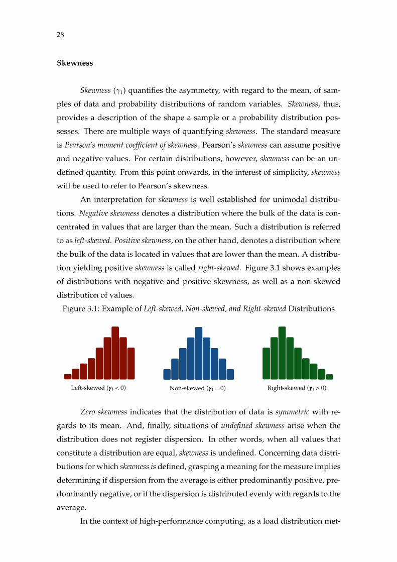
tion yielding positive skewness is called right-skewed. Figure 3.1 shows examples

of distributions with negative and positive skewness, as well as a non-skewed

distribution of values.

Figure 3.1: Example of Left-skewed, Non-skewed, and Right-skewed Distributions

Non-skewed (𝜸1 = 0) Right-skewed (𝜸1 > 0)Left-skewed (𝜸1 < 0)

Zero skewness indicates that the distribution of data is symmetric with re-

gards to its mean. And, finally, situations of undefined skewness arise when the

distribution does not register dispersion. In other words, when all values that

constitute a distribution are equal, skewness is undefined. Concerning data distri-

butions for which skewness is defined, grasping a meaning for the measure implies

determining if dispersion from the average is either predominantly positive, pre-

dominantly negative, or if the dispersion is distributed evenly with regards to the

average.

In the context of high-performance computing, as a load distribution met-

29

ric, the skewness of the distribution of computational loads across resources will

inform if either a greater number of resources register loads that are larger than

the average load (left-skewed distribution), if most resources yield loads that are

smaller than the average load (right-skewed distribution), or if load distribution

is symmetric. Skewness, then, does not provide a sense of how harsh or mild the

imbalance is. Nonetheless, the measure does provide a sense of the nature the

load distribution has.

Kurtosis

Kurtosis (γ2) is statistical measure that informs what is the nature of disper-

sion within a distribution of values. In its own way, kurtosis also is a descriptor

of the shape a distribution assumes. Several ways to estimate kurtosis exist. The

most common measure is Pearson’s moment coefficient of kurtosis. For the sake of

simplicity, kurtosis will be used to refer to Pearson’s definition from this point

forward.

Kurtosis can assume positive and negative values. Additionally, in distri-

butions where no dispersion is registered, kurtosis is unspecified. In unimodal

distributions, higher values for kurtosis communicate that the bulk of the disper-

sion within the distribution is caused by rare major deviations from the central

location (i.e. outliers). Lower values, on the other hand, indicate that dispersion

within the distribution comes from recurrent minor deviations from the average.

Due to its centrality in statistics, it is common practice to contrast the kur-

tosis of a distribution to the one registered by the normal distribution. For this

reason, kurtosis of a collection of values or a probability distribution is adjusted to

the kurtosis of univariate normal distributions by calculating a quantity known as

excess kurtosis. Excess kurtosis is defined as kurtosis minus 3, which is the kurtosis

yield by an univariate normal distribution.

Owing to the ubiquitousness of excess kurtosis as the effective measure of

kurtosis, distributions are classified according to this value. A distribution with

zero kurtosis is referred to as mesokurtic. Univariate normal distributions, regard-

less of parameter values, are always mesokurtic. Distributions of values possess-

ing negative excess kurtosis are called platykurtic. Dispersion in platykurtic distri-

butions are, when compared to the normal distribution, more a product of fre-

30

quent minor deviations from the average.

Distributions with positive excess kurtosis are classified as leptokurtic. In

leptokurtic distributions, dispersion is caused more by rare major deviations from

the mean than in normal distributions. It is fundamental to understand that kur-

tosis does not measure the magnitude of dispersion. Platykurtic distributions are

not less dispersed than mesokurtic or leptokurtic distributions. Kurtosis provides,

instead, a sense of how dispersion is produced.

Hence, three distributions yielding both the same mean and standard de-

viation could be either mesokurtic, platykurtic, or leptokurtic. In comparison to the

mesokurtic distribution, the platykurtic would have the bulk of its values scattered

over a broader area, while in the leptokurtic distribution the bulk of the values

would be concentrated closer the mean. Figure 3.2 provides a visual example of

the shape the distributions have according to their excess kurtosis.

Figure 3.2: Example of Mesokurtic, Platykurtic, and Leptokurtic Distributions

Platykurtic (𝜸2 < 0) Mesokurtic (𝜸2 = 0) Leptokurtic (𝜸2 > 0)

For the remainder of this document, kurtosis will be used to refer to excess

kurtosis. Employed as a computational load distribution metric, kurtosis specifies

whether load distribution contains either a few outliers or if it is composed by

multiple modestly imbalanced resources. As is the case with skewness, kurtosis

does not quantify the dimension of load imbalance. Instead, it provides informa-

tion on the nature of the imbalance present in the load distribution.

Summary

The majority of the metrics discussed above provide some form of quan-

tification of load imbalance severity. Metrics of load imbalance severity measure

how acute the disparities in computational load between resources is. Percent im-

balance, imbalance percentage, imbalance time, and standard deviation are all examples

31

of metrics which convey a sense of the difference between computational loads

between resources. These measures are the essence of the first step of any load

balancing procedure and are, thus, the basis upon which a decision is made by

the load balancer on whether or not to redistribute load.

Skewness and kurtosis differ from these metrics in that neither quantifies

load imbalance in itself. Each measures an attribute of the load distribution’s na-

ture without considering the magnitude of disparities in computational load be-

tween resources. For these reasons, skewness and kurtosis are not useful as guides

to determine if load rebalancing is needed. However, in the case where the sever-

ity measures have indicated that load balancing is required, these metrics provide

assistance on the decision on how load should be redistributed (PEARCE et al.,

2012).

32

4 METHODOLOGY

The methodology employed to answer the questions posed in this disser-

tation is described in this chapter. As stated earlier, the goal is to establish the

degree to which measures employed to gauge load distribution are informative

in characterizing the patterns of work allocation in parallel applications. Six com-

monly used load distribution metrics will be evaluated: percent imbalance, imbal-

ance percentage, imbalance time, standard deviation, skewness, and kurtosis.

The assessment of these metrics will involve examining how each metric

quantifies the unfolding of load distribution for a few parallel application ex-

ecutions. This procedure is expected to provide with an understanding of the

selected measures virtues and failures. The differences between the measures

should be revealed as a result of the analysis as well.

The remainder of the chapter is structured as follows. First, the process

through which the load patterns of a parallel application execution are uncov-

ered is presented in Section 4.1. Section 4.2 reveals the method employed to

evaluate the load distribution metrics. Section 4.3 ends the chapter by provid-

ing information on both the data and the tools used in the analysis presented in

this document.

4.1 Load Analysis

In order to properly describe the load analysis methodology employed in

this dissertation, first it is necessary to establish what constitutes computational

load. Load is any operation that is not communication, synchronization or any

other form of resource interaction. Hence, any given operation performed by a

resource during application execution that does not qualify as interaction with

other resources is classified as computational load associated with the resource in

question.

The total load for a resource is computed by adding the length, in seconds,

of all operations classified as computational load that were executed by this re-

source. The analysis examines the evolution of load during the complete applica-

tion execution. The evolution is grasped by splitting the execution in intervals of

equal length and determining the load distribution separately on each of them.

33

The analysis will consider the normalized load resources register at all inter-

vals into which execution was divided. The normalized load a resource yields for

a given time step consists in the ratio of the load the resource registered during

the time step by the length of the time step. The quantity is dimensionless and

represents the fraction of time that a resource has spent computing. It is therefore

bound to be within 0 and 1.

The progress of load distribution for an execution is analyzed by using a

graphical representation known as heat map1. In a heat map, values in a matrix

are represented as colors. Therefore, uncovering the load patterns of a parallel

application execution will involve examining a plot representing the progress of

load distribution through time as a heat map. Figure 4.1 exemplifies how load

evolution for a parallel application is rendered in this document.

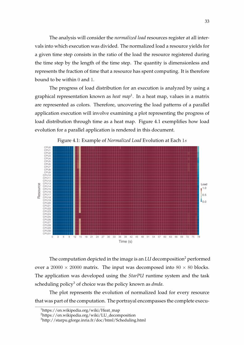
Figure 4.1: Example of Normalized Load Evolution at Each 1s

��

� � � � ��

��

��

��

��

��

��

The computation depicted in the image is an LU decomposition2 performed

over a 20000 × 20000 matrix. The input was decomposed into 80 × 80 blocks.

The application was developed using the StarPU runtime system and the task

scheduling policy3 of choice was the policy known as dmda.

The plot represents the evolution of normalized load for every resource

that was part of the computation. The portrayal encompasses the complete execu-

1https://en.wikipedia.org/wiki/Heat_map2https://en.wikipedia.org/wiki/LU_decomposition3http://starpu.gforge.inria.fr/doc/html/Scheduling.html

34

tion. The horizontal axis depicts the progression of time, starting at the moment

the application began computing and ending as soon as computation completes.

Time progression is always rendered in seconds. In the case of the execution

depicted in Figure 4.1, the computation lasted roughly 78s. The execution was

divided in 1s intervals to allow for the progress of load distribution to be ana-

lyzed.

The vertical axis contains a list, in alphabetical order, of all resources that

are part of the parallel system used for executing the application. Hence, in the

example execution under consideration, 32 processing elements participated in

the computation. A color guide is placed to the right of the image. The guide

maps the colors depicted in the heat map to normalized load values. As a result,

this guide will always range between 0 and 1. At all times, dark blue signifies

complete idleness, while dark red signals full occupation.

Interpreting Figure 4.1 is straightforward. From the beginning of the com-

putation until 11s into execution, all resources are completely idle, as the dark

blue tones indicate. Following that period of inactivity, for 1s every resource reg-

isters approximately 0.5 of normalized load. After this brief interval, apart from

a few exceptions, starting at 12s all the way through to 1s before the execution

ended, resources were fully occupied, yielding a normalized of 1.0.

The exceptions to this perfect allocation of load registered within the 12−

77s stretch of time were located in four 1s intervals. In the 13 − 14s span, the

eight CPU’s situated at the top of the heat map had loads slightly below 1.0,

while the other resources maintained the behavior from the preceding time step.

Right after, all resources but CPU24 and CPU25, which are fully occupied, yielded

loads close 0.75 in the 1s time slice starting at 14s. Later in the computation, in

the 72 − 73s and 76 − 77s intervals, a few of the resources yielded loads barely

below 1.0, as the light red hues reveal.

Finally, in the very last second of execution, resources present minor differ-

ences in computational loads. All yield low values, as the mixture of blue tones

communicates. The uppermost resource yielded a normalized load of 0.2 and

the lowest resource rendered in the plot was completely idle during this period.

Every other resource held a normalized load somewhere in between those two

values.

The length of the time steps through which the progress of an application’s

35

execution can be grasped are selected empirically. The process of selecting the

appropriate pace of evolution involves two aspects. First, for a given execution,

the time step has to be adequately large to render the depiction of normalized

load evolution for every resource discernible. Second, it also had to be sufficiently

short to depict the execution’s progress without aggregating run time information

excessively.

With the goal of illustrating the process of electing a length for the evo-

lution of load to be computed, Figure 4.2 renders the progress of computational

load across resources for a time step of 0.1s. This is the same execution as the one

depicted in Figure 4.1.

Figure 4.2: Example of Normalized Load Evolution at Each 0.1s

��

� � � � ��

��

��

��

��

��

��

The patterns of load distribution are similar to the ones seen previously,

when computational loads were determined at each 1s. However, the level of de-

tail is such that, given the limited horizontal space available in a page, identifying

and describing the load patterns with precision is a difficult task. The opposite

situation, where the length of the time slices is too large, is illustrated by Fig-

ure 4.3. The image shows the evolution of load for the same LU decomposition

computation at every 10s.

The problem that arises with a coarser representation of the evolution of

computational load is evident in the plot. An aggregation level as the one em-

ployed in Figure 4.3 has the effect of making the patterns seen in the previous

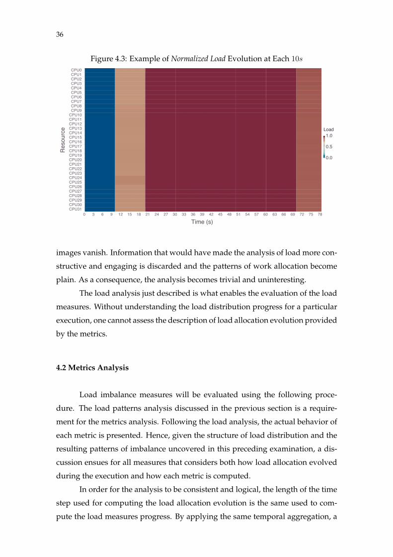
36

Figure 4.3: Example of Normalized Load Evolution at Each 10s

��

� � � � ��

��

��

��

��

��

��

images vanish. Information that would have made the analysis of load more con-

structive and engaging is discarded and the patterns of work allocation become

plain. As a consequence, the analysis becomes trivial and uninteresting.

The load analysis just described is what enables the evaluation of the load

measures. Without understanding the load distribution progress for a particular

execution, one cannot assess the description of load allocation evolution provided

by the metrics.

4.2 Metrics Analysis

Load imbalance measures will be evaluated using the following proce-

dure. The load patterns analysis discussed in the previous section is a require-

ment for the metrics analysis. Following the load analysis, the actual behavior of

each metric is presented. Hence, given the structure of load distribution and the

resulting patterns of imbalance uncovered in this preceding examination, a dis-

cussion ensues for all measures that considers both how load allocation evolved

during the execution and how each metric is computed.

In order for the analysis to be consistent and logical, the length of the time

step used for computing the load allocation evolution is the same used to com-

pute the load measures progress. By applying the same temporal aggregation, a

37

direct correlation between the load analysis and the metrics can be derived. The

purpose is to determine if measures communicate the same evolutionary behav-

ior revealed in the load analysis.

The LU decomposition computation for which the load distribution was

discussed in Section 4.1 will now be used to illustrate how metrics are depicted.

Figure 4.4 portrays the evolution of each of the six metrics which will be investi-

gated. As was the case for the load patterns depicted in Figure 4.1, the time step

length is 1s. Once more, the horizontal axis represents the passing of time, in sec-

onds. The vertical axis depicts the range of values the measure yielded. Points

indicate the value held by the metric in a given time step. A line connects all

points in chronological order to give a sense of the metrics progression through

time.

Hence, for the LU decomposition execution under analysis, at every one

second each measure was computed and its value is represented by a point. In

the interval between 2 − 11s, the absence of points designating values held for

percent imbalance, imbalance percentage, skewness, and kurtosis informs that these

metrics were undefined during this period of time.

Considering that the metrics can be separated in two groups based on the

load distribution aspect they quantify, the analysis of the measures is performed

separately for each group. First, the measures of load imbalance severity are con-

sidered. This group is composed by percent imbalance, imbalance percentage, imbal-

ance time, and standard deviation. Analysis of skewness and kurtosis, which gauge

the load distribution shape, is performed afterwards.

Since the measures within each group have similar objectives, clustering

the analysis in these groups avoids excessive repetitiveness as the expectations

and the behavior within a group are alike and, thus, can be revealed together. Fur-

thermore, such an arrangement facilitates the comparison of metrics with their

group peers.

At all times, the severity metrics are normalized to be within a common

scale and, consequently, simplify comparisons between them. For each of the

four measures, each value yielded for every time step is adjusted to be within 0

and 1. This is accomplished through the division of the value registered in each

time step by the maximum value that the measure could possibly yield.

Hence, the values displayed in Figure 4.4 for percent imbalance, imbalance

38

Figure 4.4: Example of Metrics Evolution at Each 1s

��

� � � � ��

�

��

��

��

� � � � ��

��

��

�

�

��

� � � � ��

��

��

��

��

� � � � ��

��

��

��

��

� � � � ��

��

��

��

��

� � � � ��

��

��

��

percentage, imbalance time, and standard deviation denote the fraction of the highest

value each measure can register for the time step length employed in the analysis.

Therefore, for instance, in the first time step, percent imbalance registered approx-

imately 11% of the maximum value possible for the measure, while for the last it

yielded 6% of the metric highest value for a 1s time step.

As a consequence of the normalization, both imbalance time and standard

deviation, which are quantified in the same unit of measure as is the computa-

tional load, become dimensionless. Percent imbalance and imbalance percentage are

39

by definition dimensionless and, evidently, remain dimensionless after normal-

ization. Since skewness and kurtosis can yield both positive and negative values,

the values registered by these metrics were not normalized, as that would result

in a loss of valuable information regarding the load distribution.

For the load analysis described in the previous section, the load values are

normalized prior to being rendered in the heat map. This does not mean that the

measures are computed based on these normalized values. Load values in sec-

onds registered by each resource, and not normalized load, are used to determine

the metrics values for any given interval.

The combination of the analysis of load patterns, described in Section 4.1,

and the measures analysis, detailed above, is what constitutes the process em-

ployed to evaluate the load distribution measures selected for this study. Both

components of the methodology rely on visual analysis of the images chosen to

depict load distribution evolution and the measures description of this evolution.

Associating the patterns portrayed by both images allows for the advantages and

disadvantages of the measures to be exposed.

4.3 Data & Tools

The analysis described Sections 4.1 and 4.2 is post-mortem or, in other words,

performed after the application has finished its execution. Information regarding

the computational load registered by every resource participating in the execu-

tion is gathered from execution traces. The traces are stored in files that register

events as comma-separated values (CSV) which were obtained by converting Pajé

trace files4 using the PajeNG5 toolset.

YAJP.jl6, a package developed using the Julia programming language7, is

employed to generate the images used in both the load and metrics analysis. The

package contains methods to parse, extract, and analyze information contained

in Pajé execution traces exported as CSV files.

All execution traces used in this study, as well as the images depicting load

distribution patterns and the evolution of load metrics for these executions, are

4http://paje.sourceforge.net/download/publication/lang-paje.pdf5https://github.com/schnorr/pajeng6https://github.com/flavioalles/YAJP.jl7http://julialang.org

40

public8. The script used to generate all plots is also available in the repository.

Both the Julia environment and YAJP.jl are required for the script to be run suc-

cessfully. For more details, refer to the README file located in the repository.

8https://github.com/flavioalles/data

41

5 EXPERIMENTAL RESULTS AND ANALYSIS

Experimental results and analysis for this study into load distribution mea-

sures are presented in this chapter. As outlined in Chapter 4, six different metrics

commonly used as scales to gauge load distribution in parallel applications are

investigated: percent imbalance, imbalance percentage, imbalance time, standard devia-

tion, skewness, and kurtosis.

The structure of chapter is as follows. Section 5.1 contains information re-

garding the experiments conducted for the study. Both the computing platform

and the case studies used to perform the evaluation are described. Subsequently,

the load distribution measures are evaluated in Section 5.2. A discussion summa-

rizing the findings of the analysis ends the chapter in Section 5.3.

5.1 Experimental Setup: Platform Configuration and Case Studies

The experimental platform on which executions used to perform the mea-

sures evaluation is described in Section 5.1.1. Two applications were used as case

studies for this dissertation. The first was a seismological simulator called On-

des3D. The second application performs a a linear algebra operation known as a

Cholesky decomposition. In Section 5.1.2, the Ondes3D simulator is explained. A

discussion on the Cholesky decomposition follows in Section 5.1.3.

5.1.1 Experimental Platform

All experiments conducted for this research effort were executed on the

Turing machine, which is owned and maintained by the Grupo de Processamento

Paralelo e Distribuído of the Instituto de Informática/UFRGS. The machine is a single-

node homogeneous multi-processor computer. Turing’s computing power stems

from four Intel Xeon X7550 processors. The processor’s standard frequency is

2GHz and the maximum rate in which it can operate is 2.4GHz. The Xeon X7550

is a multi-core processor containing 8 identical processing units, which combined

within the Turing machine total 32 processor cores.

Simultaneous multi-threading, where multiple independent threads of ex-

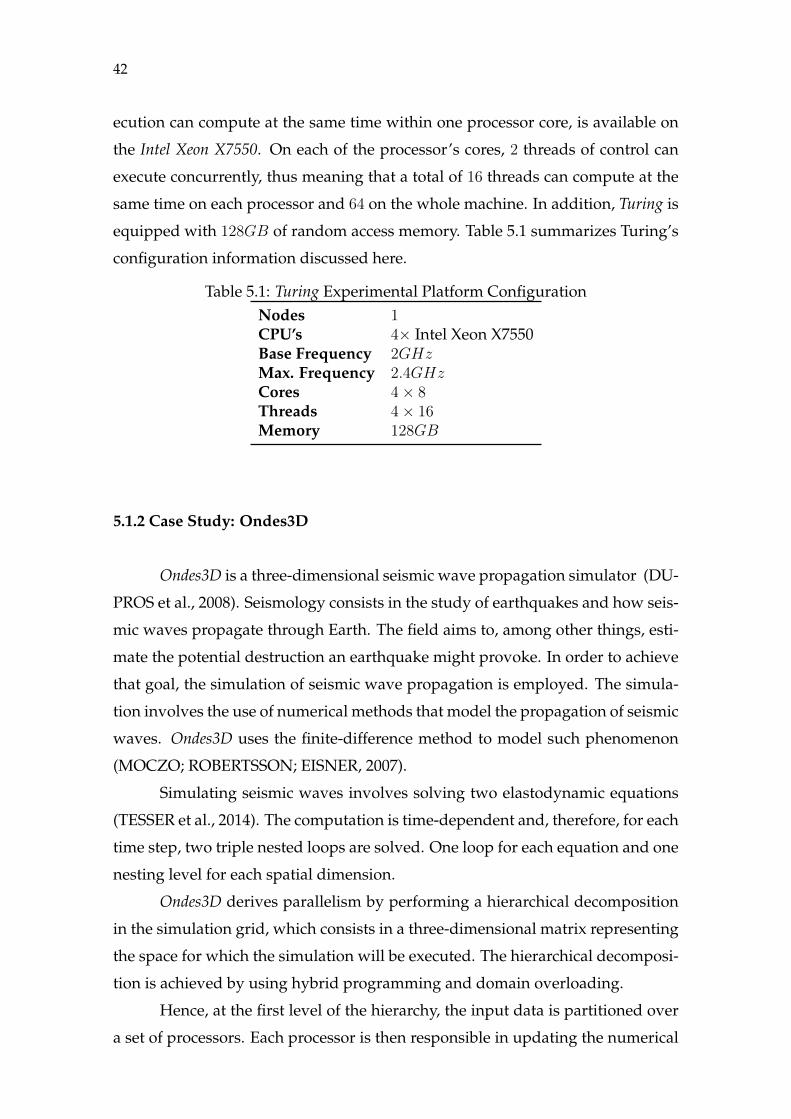
42

ecution can compute at the same time within one processor core, is available on

the Intel Xeon X7550. On each of the processor’s cores, 2 threads of control can

execute concurrently, thus meaning that a total of 16 threads can compute at the

same time on each processor and 64 on the whole machine. In addition, Turing is

equipped with 128GB of random access memory. Table 5.1 summarizes Turing’s

configuration information discussed here.

Table 5.1: Turing Experimental Platform ConfigurationNodes 1CPU’s 4× Intel Xeon X7550Base Frequency 2GHzMax. Frequency 2.4GHzCores 4× 8Threads 4× 16Memory 128GB

5.1.2 Case Study: Ondes3D

Ondes3D is a three-dimensional seismic wave propagation simulator (DU-

PROS et al., 2008). Seismology consists in the study of earthquakes and how seis-

mic waves propagate through Earth. The field aims to, among other things, esti-

mate the potential destruction an earthquake might provoke. In order to achieve

that goal, the simulation of seismic wave propagation is employed. The simula-

tion involves the use of numerical methods that model the propagation of seismic

waves. Ondes3D uses the finite-difference method to model such phenomenon

(MOCZO; ROBERTSSON; EISNER, 2007).

Simulating seismic waves involves solving two elastodynamic equations

(TESSER et al., 2014). The computation is time-dependent and, therefore, for each

time step, two triple nested loops are solved. One loop for each equation and one

nesting level for each spatial dimension.

Ondes3D derives parallelism by performing a hierarchical decomposition

in the simulation grid, which consists in a three-dimensional matrix representing

the space for which the simulation will be executed. The hierarchical decomposi-

tion is achieved by using hybrid programming and domain overloading.

Hence, at the first level of the hierarchy, the input data is partitioned over

a set of processors. Each processor is then responsible in updating the numerical

43

model concerning its portion of the grid and in exchanging information with the

neighboring portion of grid. Ondes3D uses the MPI framework as the paralleliza-

tion framework for the first level of decomposition.

Within each portion of the grid mapped into a processor, a second layer

of parallelism is introduced. Each sub-domain (i.e. process) is partitioned into

a number of smaller domains (i.e. threads) greater than the number of virtual

processors. The overloading strategy at the second level of decomposition aims to

profit from potential cache effects and to address load-balancing problems at the

first level of partitioning. The hierarchical decomposition performed by Ondes3D

is illustrated in Figure 5.1.

Figure 5.1: Ondes3D Hierarchical Decomposition

MPI Threads

Since the experimental platform has 32 physical cores (see Table 5.1), in

the Ondes3D executions performed for this study, the first level of decomposition

involved partitioning the simulation grid into 32 MPI processes. For this appli-

cation, MPI operations are discarded and any other activity is considered to be

computational load.

5.1.3 Case Study: Cholesky Decomposition

In mathematics, decomposition or factorization denotes the operation of

decomposing an object into a product of other objects, referred to as factors. In

linear algebra, the object decomposed through such an operation is a matrix and,

as a result, the factors into which a matrix is decomposed are matrices as well.

A Cholesky decomposition is the decomposition of a Hermitian1 positive-

definitive2 matrix into the product of a lower triangular matrix3 and its conjugate

1https://en.wikipedia.org/wiki/Hermitian_matrix2https://en.wikipedia.org/wiki/Positive-definite_matrix3https://en.wikipedia.org/wiki/Triangular_matrix

44

transpose4. The decomposition is primarily employed to solve certain systems of

linear equations more efficiently. Figure 5.2 illustrates the operation performed

in a Cholesky decomposition.

Figure 5.2: Cholesky Decomposition

= x

HermitianPositive-definite Lower Triangular Lower Triangular

Conjugate Transpose

The Cholesky decomposition application used as a case study for this dis-

sertation is developed using StarPU (AUGONNET et al., 2009). StarPU is a task

programming library for heterogeneous architectures. The application developed

with the library is expected to provide the implementations of tasks on every ar-

chitecture where these tasks are supposed to run (i.e. CPU, GPU) and the task-

dependency graph.

Given these inputs, StarPU’s runtime system is responsible in enforcing

the dependencies between different tasks, scheduling tasks into the most ap-

propriate resource according to a given policy and handling data transfers be-

tween resources. Hence, StarPU performs dynamic mapping over heterogeneous

resources and transparently manages the movement of data between these re-

sources.

The Cholesky decomposition application used here is shipped as an exam-

ple application with StarPU’s official release. The user of the application has the

option of indicating the size of the matrix upon which the factorization ought to

be performed, as well as the size of the blocks into which the input is partitioned.

The scheduling policy used during execution can also be determined. For the

executions performed for this dissertation, the dmda5 was the policy of choice.

Several types of operations where recorded in the execution traces of this

application. For most of these operations, their purpose can be recognized sim-

4https://en.wikipedia.org/wiki/Conjugate_transpose5http://starpu.gforge.inria.fr/doc/html/Scheduling.html

45

ply by reading the name with which they are recorded in the traces. Therefore,

records with the following identifiers are considered computational load for the

purposes of the analysis performed in this document: cl11, cl21, cl22, cl22_p, Call-

back and Scheduling. Operations that are not regarded as load are: Idle, Initializing,

FetchingInput, PushingOutput, Overhead, and Sleeping.

The operations identified as cl11, cl21, cl22, and cl22_p are the tasks pro-

vided by the developers of the application performing the actual Cholesky de-

composition. Every other operation is related to handling the runtime concerns

associated with executing a parallel application.

None of the Cholesky decomposition executions made use of the simultane-

ous multi-threading technology provided by the experimental platform. Hence,

StarPU’s runtime system pinned one worker processes (i.e resource into which

tasks are assigned) in each of the physical processor cores available in the Turing

machine. Therefore, the total number of resources at the disposal of the the task

scheduler was 32.

5.2 Metrics Analysis

The investigation into the load distribution measures will now follow. The

section is divided in two parts, one for each of the applications selected as case

studies. First, in Section 5.2.1, analysis is performed using the Ondes3D seismical

wave propagation simulator. Afterwards, in Section 5.2.2, load distribution mea-

sures are investigated for executions of the Cholesky decomposition developed

with the StarPU task programming library.

In each execution used as the means through which metrics are examined,

analysis involves first uncovering load patters and then analyzing load measures.

The analysis of metrics is performed in two separate parts. The evolution of per-

cent imbalance, imbalance percentage, imbalance time, and standard deviation is dis-

cussed first. Afterwards, skewness and kurtosis are examined.

46

5.2.1 Ondes3D

Two executions of the Ondes3D seismic wave propagation simulator are

the base upon which load distribution measures analysis will be conducted in this

section. These executions differ in the way communications between processes

are performed. In the first, synchronous (i.e. blocking) communication was em-

ployed, while in the second Ondes3D run, communication between processes was

exclusively asynchronous (i.e. non-blocking). Load and metrics analysis for the

blocking version of Ondes3d is presented in Section 5.2.1.1. For the non-blocking

variation of the simulator, analysis is available in Section 5.2.1.2.

5.2.1.1 Blocking

Figure 5.3 depicts the complete evolution of the normalized load per re-

source for the Ondes3D/Blocking execution. From the image, it can be deduced

that the application completed in, approximately, 88s. The empirically deter-

mined time step length adopted to portray the progress of resource loads was

1s. Based on the patterns displayed on the image, a description of how load dis-

tribution evolved for this particular Ondes3D execution will now follow.

Figure 5.3: Ondes3D/Blocking Normalized Load Evolution at Each 1s

��

� � � � ��

��

��

��

��

��

��

47

Load Analysis

In terms of load distribution, the execution can be divided in 6 stages. The

first stage, which lasts only 1s, is characterized by resources being completely, or

almost completely, idle as the dark blue tones indicate. A 2s interval (1 − 3s),

where load is slightly more imbalanced, follows. During this stretch, resources

at the top of the plot yield normalized loads of approximately 0.75, while the rest

register load levels around 0.5.

The third stage of the execution, starting at 3s and spanning until the 35s

mark, is a period where workload is almost equal across all resources, as the

homogeneous coloring suggests. Resource loads alternate between 0.5 and 0.6

with a certain regularity, indicating that this 32s interval records only minor load

imbalance. Next there is a 4s span (35−39s) where two of the processes, rank5 and

rank13, exhibit a surge in their normalized loads. Both are almost fully utilized

in the time slices encompassing this interval, while the other processes retain the

behavior presented in the previous stage.

The following phase of computation (39 − 87s) resembles the 3 − 35s pe-

riod. Load is balanced and resources are operating at around half of their capac-

ity. These two stages, which are similar in their nature, dominate the execution

amounting to 80s or close to 91% of the total run time. The last stage of execution,

with regards to load distribution, starts at 87s and lasts less than 2s. This interval

represents a period of evident load imbalance, with the resources located at the

uppermost portion of the plot experiencing a decrease in their normalized loads.

Percent Imbalance, Imbalance Percentage, Imbalance Time, and Standard Deviation

Considering the load patterns exposed above, the progress of the load im-

balance severity measures will now be examined. The evolution, computed in 1s

time steps, of the four metrics of load imbalance severity for the Ondes3D/Blocking

run under analysis is shown in Figure 5.4. As discussed in Chapter 4, the mea-

sures have been normalized to be within 0 and 1.

In the first phase of execution (0− 1s), in which loads are almost the same

for all processor cores, imbalance time and standard deviation indicate that load im-

balance is modest by yielding values close to zero. For both metrics, this is the

lowest value registered during the execution. The other two measures that com-

48

Figure 5.4: Ondes3D/Blocking Severity Metrics Evolution at Each 1s

��

� � � � ��

��

��

��

��

� � � � ��

��

��

��

��

� � � � ��

��

��

��

��

� � � � ��

��

��

��

pute the severity of dispersion, on the other hand, produce the highest values of

load imbalance for this Ondes3D execution within this period. The differences

in magnitude between them are vast, nonetheless. While percent imbalance yields

only a modest below 6% of the maximum possible value, imbalance percentage as-

signs a value that is slightly over 65% of its severity scale.

Given the increased levels of load registered for a few of the processes at

the top of Figure 5.3, the 2s interval following this first stage of execution was

expected to report load imbalance, as measured by each of these four metrics, at

higher levels than the preceding and succeeding periods. However, none of the

measures yielded values that are significantly different from what is registered in

49

the following stretch of execution.

The third (3−35s) and fifth (39−85s) execution phases, two long periods of

relatively stable load balance yield, as expected, low values for percent imbalance,

imbalance percentage, imbalance time, and standard deviation. Considering the mod-

est oscillations load resources register in these periods, the minor variations the

metrics register were expected. However, even though the behavior for each of

the four measures for both intervals is similar, it is not identical. For the 3−35s in-

terval, load imbalance oscillates more than for the 39−87s stretch. This difference

in behavior is unexpected, considering that both intervals have nearly identical

load patterns in Figure 5.3.

The fourth phase (35 − 39s), which registers an imbalance due to a sharp

load increase in two resources, while the other 30 cores maintain the load patterns

from the previous period, produced an increase in all load imbalance severity

metrics, as expected. However, this increase in load imbalance, as measured by

each metric, is not identical for all four metrics.

The rise in load imbalance as reported by percent imbalance, imbalance per-

centage, and standard deviation is relatively smaller, in view of the fact that these

metrics are less prone to outliers. Conversely, given that imbalance time is deter-

mined by computing the difference between maximum and average load, this

metric is more affected by extreme behavior and the increase in value for this

measure is more pronounced within this 4s interval. While the surge in imbalance

time was nearly fivefold, the other three measure rose three times, approximately,

when compared to the preceding time step.

The last interval of execution (87 − 88s) presented a noticeable imbalance

as well. Percent imbalance, imbalance percentage, and standard deviation properly

communicate this load dispersion as the rise in its values indicate. Imbalance time

reports an increased imbalance for this period as well, although at a smaller mag-

nitude than the other measures.

Skewness and Kurtosis

The evolution of skewness and kurtosis will now be examined. Figure 5.5

shows the progress at every 1s for both shape metrics during the Ondes3D/Blocking

run under analysis.

Skewness oscillates within values close to zero for the two large periods of

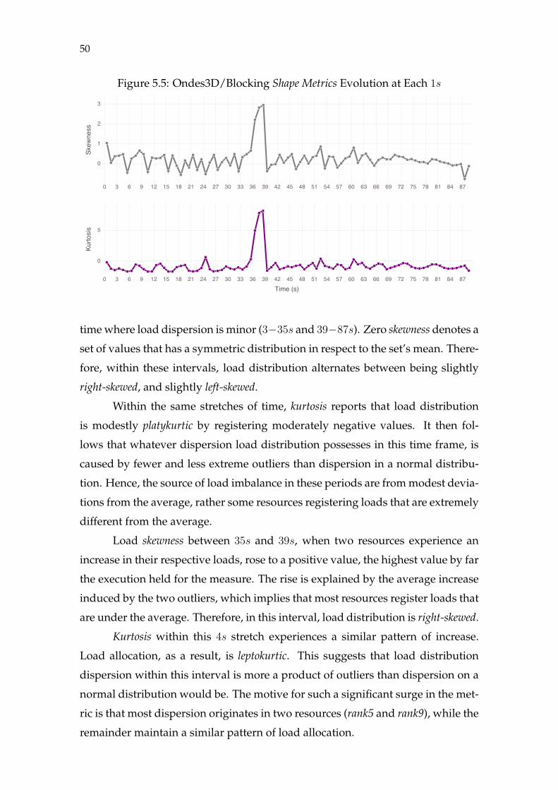
50

Figure 5.5: Ondes3D/Blocking Shape Metrics Evolution at Each 1s

��

� � � � ��

�

�

��

� � � � ��

�

�

�

�

��

time where load dispersion is minor (3−35s and 39−87s). Zero skewness denotes a

set of values that has a symmetric distribution in respect to the set’s mean. There-

fore, within these intervals, load distribution alternates between being slightly

right-skewed, and slightly left-skewed.

Within the same stretches of time, kurtosis reports that load distribution

is modestly platykurtic by registering moderately negative values. It then fol-

lows that whatever dispersion load distribution possesses in this time frame, is

caused by fewer and less extreme outliers than dispersion in a normal distribu-

tion. Hence, the source of load imbalance in these periods are from modest devia-

tions from the average, rather some resources registering loads that are extremely

different from the average.

Load skewness between 35s and 39s, when two resources experience an

increase in their respective loads, rose to a positive value, the highest value by far

the execution held for the measure. The rise is explained by the average increase

induced by the two outliers, which implies that most resources register loads that

are under the average. Therefore, in this interval, load distribution is right-skewed.

Kurtosis within this 4s stretch experiences a similar pattern of increase.

Load allocation, as a result, is leptokurtic. This suggests that load distribution

dispersion within this interval is more a product of outliers than dispersion on a

normal distribution would be. The motive for such a significant surge in the met-

ric is that most dispersion originates in two resources (rank5 and rank9), while the

remainder maintain a similar pattern of load allocation.

51

Finally, in the last stage of execution (87 − 88s), both skewness and kurtosis

are negative, denoting that load distribution is left-skewed and platykurtic. Conse-

quently, most of the resources yield loads that are higher than the average load

within this period. The values are smaller in magnitude than in the 35 − 39s

stretch, reflecting the less acute asymmetry seen in these period. Negative kurto-

sis is communicating that dispersion is consequence of frequent minor deviations

from the mean. Both measures coherently describe the pattern seen in Figure 5.3

for this last execution phase.

Discussion

Percent imbalance and imbalance percentage reported the highest levels of

load imbalance in the first second of the execution. Within this small time frame,

all resources register almost inexistent activity. Considering the complete exe-

cution, this corresponds to the period where load dispersion is probably at its

lowest.

The second highest value recorded for each of these two metrics occurred

in the last second of execution. Normalized percent imbalance was approximately

0.04, or two-thirds of the value computed in the first time step. Imbalance percent-

age registered 0.58, 90% of the value yielded in the 0− 1s interval. Given that the

last second clearly has a more imbalanced load distribution, the behavior of both

percent imbalance and imbalance percentage for this brief interval where resources

are either idle or registering very little activity is peculiar.

None of the load imbalance severity measures produced the expected be-

havior in the 2s stretch starting at 1s and ending 3s into execution. For percent

imbalance imbalance percentage, and imbalance time load imbalance is only mod-

estly higher than most of the succeeding interval. Additionally, these measures

register a higher value of load imbalance for the 31 − 32s interval, which in Fig-

ure 5.3 does not give the impression of retaining increased load dispersion than

the interval in question. Standard deviation records a higher value for the period

than every time step in the 3 − 35s span. However, the difference is minor and,

as a consequence, does not seem to reflect the load patterns revealed for these

intervals.

All four severity measures yielded different behaviors for the two periods

of time where load patterns are similar. Intervals 3 − 35s and 39 − 85s present

52

load allocation patterns that are almost identical, as Figure 5.3 shows. The four

measures behave in the same manner. For the first of these intervals, they report

that load imbalance varies more than in the second interval. Also, the first inter-

val yields the smallest values. For all metrics, load imbalance achieves greater

stability right before the 66s mark.

Figure 5.4 informs that standard deviation varies less than the other three

measures. By being less affected by the outliers resources during the 35 − 39s

period than imbalance time and by not registering a high level of imbalance in the

first time step of the computation, as imbalance percentage did, standard deviation

has a tighter range of values it assumes. The measure varies within 0 − 30% of

its maximum possible value. Imbalance percentage and imbalance time, on the other

hand, assume values within a wider span of values of their respective potential

range (10− 65% and 0− 50%, respectively).

Percent imbalance, however, does yield a relative variation from lowest to

highest load imbalance that is smaller that all the other metrics. The metric as-

sumes a fairly small scale of values, yielding values between 0 − 0.06 in the nor-

malized range. When compared to the other measures, the difference is con-

siderable. Between 35 − 39s, a period where a clear situation of imbalance is

observed, imbalance percentage, imbalance time, and standard deviation register nor-

malized values of 0.55, 0.5, and 0.3, approximately. Percent imbalance, on the other

hand, yields only 0.035.

Bringing the discussion of metrics coherence to an end for this Ondes3D

execution, a comment on the outline of the curves recorded for each measure.

Both the measures of imbalance severity and of the shape of the load distribu-

tion present similar patterns of variation for most of the execution, apart from

differences in the magnitude of increases and decreases in values. All register an

increase within the 35 − 39s span. The period immediately before this 4s yields

more oscillations than the period immediately after. And all measures witness a

stabilization right before the 66s mark.

5.2.1.2 Non-blocking

The evolution of the normalized load per core of another Ondes3D sim-

ulator execution is illustrated in Figure 5.6. The use of asynchronous (i.e. non-

blocking) communication primitives is what differentiates this execution from

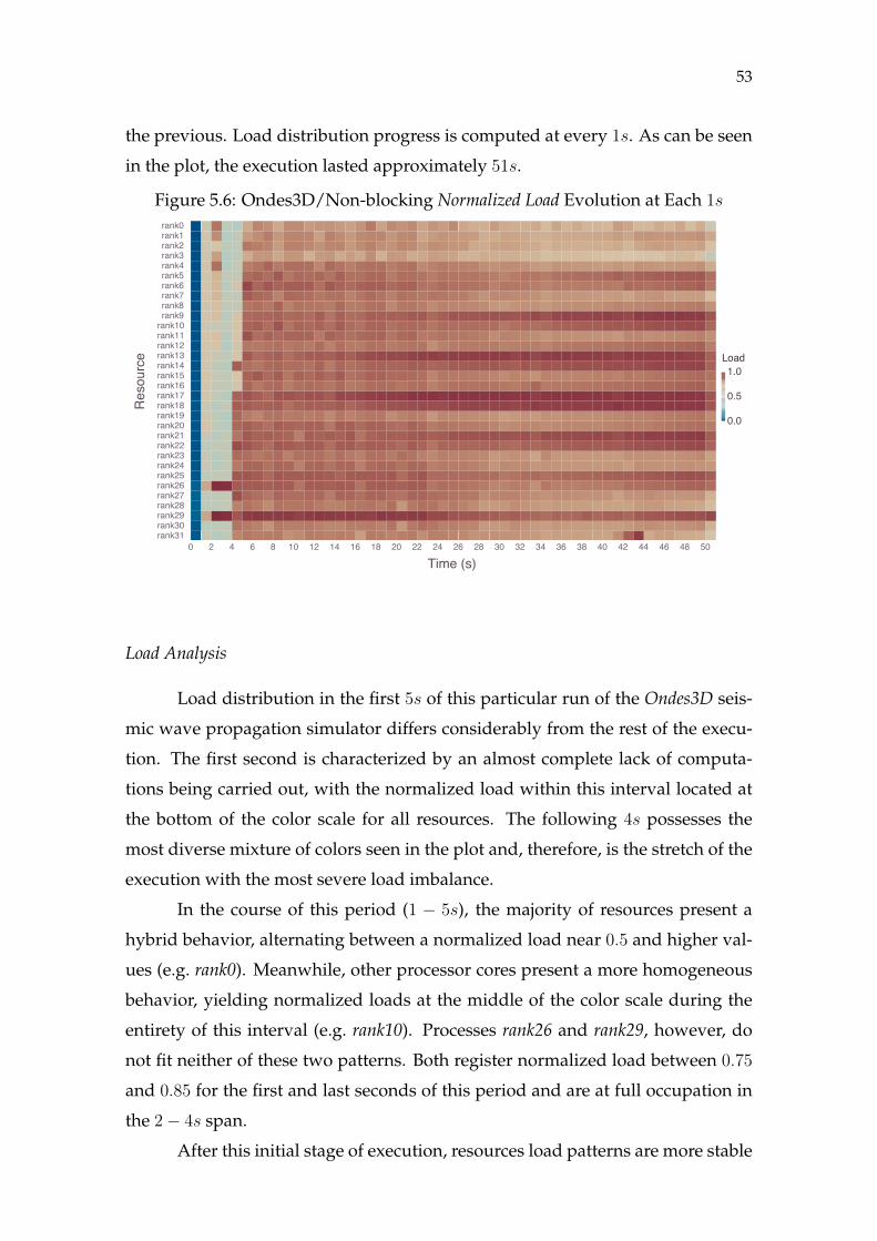
53

the previous. Load distribution progress is computed at every 1s. As can be seen

in the plot, the execution lasted approximately 51s.

Figure 5.6: Ondes3D/Non-blocking Normalized Load Evolution at Each 1s

��

� � � � � ��

��

��

��

��

��

��

Load Analysis

Load distribution in the first 5s of this particular run of the Ondes3D seis-

mic wave propagation simulator differs considerably from the rest of the execu-

tion. The first second is characterized by an almost complete lack of computa-

tions being carried out, with the normalized load within this interval located at

the bottom of the color scale for all resources. The following 4s possesses the

most diverse mixture of colors seen in the plot and, therefore, is the stretch of the

execution with the most severe load imbalance.

In the course of this period (1 − 5s), the majority of resources present a

hybrid behavior, alternating between a normalized load near 0.5 and higher val-

ues (e.g. rank0). Meanwhile, other processor cores present a more homogeneous

behavior, yielding normalized loads at the middle of the color scale during the

entirety of this interval (e.g. rank10). Processes rank26 and rank29, however, do

not fit neither of these two patterns. Both register normalized load between 0.75

and 0.85 for the first and last seconds of this period and are at full occupation in

the 2− 4s span.

After this initial stage of execution, resources load patterns are more stable

54

and less diverse. However, load imbalance is present, even if at a lesser degree.

For the remainder of time, in the interval starting at 5s and ending when execu-

tion concludes, resources assume red or light yellow tones, which indicate nor-

malized loads between 0.75 and 1.0. Hence, although for most of its execution,

this Ondes3D/Non-blocking run presents better load balancing than in the initial

5s, it still registers perceptible load disparities between resources.


The evolution for percent imbalance, imbalance percentage, imbalance time, and

standard deviation throughout this seismic wave simulator execution is shown in

Figure 5.7. Consistent with the load patterns analysis above, load imbalance

severity measures are computed for every 1s interval.

Considering the load progress presented in Figure 5.6, the first second of

the execution is the one with the least severe load dispersion, when resources are

almost completely idle. Thus, that small time frame should yield the lowest load

imbalance according to percent imbalance, imbalance percentage, imbalance time, and

standard deviation.

However, percent imbalance and imbalance percentage report that load im-

balance is at its highest levels for this Ondes3D execution within this 1s interval.

Imbalance time and standard deviation, on the other hand, signal that this is the

moment where load imbalance is smaller than anywhere else within the compu-

tation.

The highest value for load imbalance during this Ondes3D execution, as

determined by these four measures, should occur in the four second interval be-

tween 1s and 5s into execution, given that this is the period where load imbalance

is most severe. As forecast, within the first few seconds of the computation, more

precisely between 2s and 4s, peak load imbalance is reached for the execution

according to imbalance time and standard deviation. Percent imbalance and imbalance

percentage also express that this is a period of higher load dispersion, compared

to the remainder of the execution.

However, measures oscillate in different ways within this period. Imbal-

ance time, the metric most affected by outliers, yields the greatest relative increase

in load imbalance in the 2−4s interval, where two processor cores have a normal-

ized load of 1.0, while the other resources yield normalized load at the middle of

55

Figure 5.7: Ondes3D/Non-blocking Severity Metrics Evolution at Each 1s

��

� � � � � ��

��

��

��

��

� � � � � ��

��

��

��

��

� � � � � ��

��

��

��

��

� � � � � ��

��

��

��

the scale. The metric surges from a normalized value of 0.15, before the 2s mark,

to approximately 0.48 4s into execution, a threefold increase.

Within the same time frame, imbalance percentage, and standard deviation,

registered twofold increases. Percent imbalance, on the other hand, does produce a

similar threefold increase. However, the magnitude of the imbalance according to

measure is the smallest by far. Imbalance time, thus, not only registers the biggest

surge in value, but registers a higher normalized value for this period where load

dispersion is caused mostly by the outlier processes.

An interesting development seen in this period of the execution is load

imbalance decreasing for the 4 − 5s time step in comparison to the preceding

56

recorded value, according to percent imbalance, imbalance percentage, and imbalance

time, while increasing according to standard deviation. The dispersion seen within

this period is more severe according to standard deviation than the for the other

metrics. Standard deviation assigns a normalized load imbalance over 0.3 to this

time slice, while imbalance percentage and imbalance time yield 0.2.

Since there is a relative uniformity in the color tones throughout the rest

of the execution, load imbalance gauged by these metrics displays a certain sta-

bility at lower levels of the scale in this interval (5 − 51s). As the time advances,

however, load imbalance increases modestly due to a sustained growth in nor-

malized load in some of the resources (e.g. rank9, rank13, rank17), while others

maintain relatively constant load for the remainder of the execution (e.g. rank8,

rank15, rank20).

The moderate but perceptible rise in percent imbalance, imbalance percent-

age, imbalance time, and standard deviation is an indicative of a wider gap between

highest and average normalized loads. The three latter measures assign a similar

relative magnitude to load imbalance, yielding values close to 0.1.


Skewness and kurtosis progress as load distribution measures for the Ondes3D/Non-

blocking execution is seen in Figure 5.8. The metrics were computed for every 1s

interval in the course of the computation under analysis. Results for skewness will

be considered first, followed by an analysis for the evolution of kurtosis.

Given that the pattern of load distribution registered in the first second

of execution is not seen anywhere else in the computation, this brief period of

time deserves to be considered on its own. From Figure 5.6, it is clear that all but

four resources register complete inactivity (rank26, rank27, rank28, and rank29).

These four processes, however, present lighter tones of blue, which inform that

their normalized loads are moderately absolute idleness. Therefore, it is evident

that most resources loads are, in fact, below the average and, as a consequence,

load distribution is right-skewed. Also, kurtosis assigns a positive value to load

distribution within this time frame, properly communicating that dispersion is

explained by a few outliers diverging from the average.

Following this initial span, the 4s interval spanning from 1s to 5s, the as-

sumption is for load skewness to convey that there are noteworthy asymmetries in

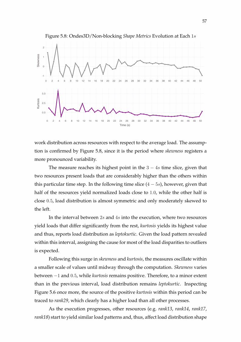
57

Figure 5.8: Ondes3D/Non-blocking Shape Metrics Evolution at Each 1s

��

� � � � � ��

��

��

��

��

� � � � � ��

��

�

�

�

��

work distribution across resources with respect to the average load. The assump-

tion is confirmed by Figure 5.8, since it is the period where skewness registers a

more pronounced variability.

The measure reaches its highest point in the 3 − 4s time slice, given that

two resources present loads that are considerably higher than the others within

this particular time step. In the following time slice (4− 5s), however, given that

half of the resources yield normalized loads close to 1.0, while the other half is

close 0.5, load distribution is almost symmetric and only moderately skewed to

the left.

In the interval between 2s and 4s into the execution, where two resources

yield loads that differ significantly from the rest, kurtosis yields its highest value

and thus, reports load distribution as leptokurtic. Given the load pattern revealed

within this interval, assigning the cause for most of the load disparities to outliers

is expected.

Following this surge in skewness and kurtosis, the measures oscillate within

a smaller scale of values until midway through the computation. Skewness varies

between −1 and 0.5, while kurtosis remains positive. Therefore, to a minor extent

than in the previous interval, load distribution remains leptokurtic. Inspecting

Figure 5.6 once more, the source of the positive kurtosis within this period can be

traced to rank29, which clearly has a higher load than all other processes.

As the execution progresses, other resources (e.g. rank13, rank14, rank17,

rank18) start to yield similar load patterns and, thus, affect load distribution shape

58

measures. Skewness presents a relatively uniform and slightly positive value de-

noting only minor asymmetries in load distribution, before decreasing modestly

at the end of execution.

With regards to kurtosis, load distribution modifies its status and is defini-

tively platykurtic from 28s onwards, when the value for the metric stays below

zero until 1s before execution completes. Hence, this denotes that the dispersion

within resource loads reported by the severity measures earlier, when compared

to normal distribution dispersion, is more a product of slight deviations from the

mean than extreme outliers.

Discussion

In conformity with what occurred in the previous execution of Ondes3D,

discussed in Section 5.2.1.1, both percent imbalance and imbalance percentage reg-

istered load imbalance severity of greater magnitude than anywhere else for a

stretch of time where differences among resources in their load levels was al-

most inexistent. The common denominator between these intervals in each of the

executions is the load yielded by resources signaled either complete or almost

complete idleness.

Percent imbalance registering smaller values when compared to the other

three measures of imbalance severity was another reoccurrence from the Ondes3D

execution analyzed in the previous section. While percent imbalance, imbalance

percentage, and imbalance time yielded maximum approximate normalized values

of 0.7, 0.5, and 0.35, respectively, percent imbalance recorded its highest value at

around 0.07.

The 4s interval (1−5s) which yields higher levels of load imbalance accord-

ing to all severity measures presents an opportunity to consider the differences

between percent imbalance, imbalance percentage, imbalance time, and standard devia-

tion. Examining Figure 5.7 closely, it becomes evident that the measures rise and

fall at different times. Percent imbalance, imbalance percentage, and imbalance time

all agree that the 3 − 4s time step is the most severely imbalanced period within

this stretch. Standard deviation, on the other hand, assigns a higher value for both

the 2− 3s and 4− 5s intervals.

Outlining the load patterns seen in Figure 5.6 for these time steps will help

to establish what distinguishes standard deviation from the other measures. The

59

2− 3s stretch presents peak load in two resources, normalized load values above

0.7 in 11 of the remaining 30 cores, while the rest register 50% occupation. In the

following period (3−4s), except for the two resources still yielding 1.0 normalized

load, all the other MPI processes yield around 0.5 load. The final time step of the

interval under consideration (4 − 5s) resembles to a certain degree the 2 − 3s

interval. Half of the resources record normalized loads over 0.75 while the rest is

either at 0.5 or modestly above.

Therefore, standard deviation is less prone to assign higher values for peri-

ods where all but a few resources present computational loads that are consider-

ably different than the majority. The measure registers higher values for periods

where load patterns are more diverse, even if the difference between most and

least loaded resources is smaller.

In any parallel computation, however, the case where load imbalance is

considered to be most severe is the one where a single resource is assigned all

computational load, while the other resources remain idle. Hence, considering

the number of resources available (32) and the time step length employed (1s),

this worst case scenario would be analogous to a single resource yielding a com-

putational load of 1.0s, while the other 31 register 0.0s.

In this situation, percent imbalance, imbalance percentage, and imbalance time

yield their highest possible values. Standard deviation, on the other hand, would

yield a value that represents 17% of its maximum possible value, which is less

than what it registers in other situations for this execution. Therefore, standard de-

viation differs from the common sense in parallel computing on what constitutes

the worst possible load distribution scenario.

5.2.2 Cholesky

In this section, analysis of load imbalance measures is performed on two

executions of a dense linear algebra application, a Cholesky factorization devel-

oped using the StarPU task programming environment. The difference between

the executions is the size of the blocks into which the input, a 20000×20000 single

precision floating point matrix, is decomposed in order for the computation to be

parallelized. In the first run (Subsection 5.2.2.1), the input is broken into 20 × 20

matrices, while in the second (Subsection 5.2.2.2), the input is split into 80 × 80

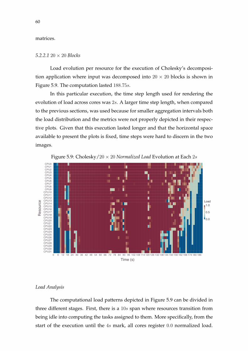
60

matrices.

5.2.2.1 20× 20 Blocks

Load evolution per resource for the execution of Cholesky’s decomposi-

tion application where input was decomposed into 20 × 20 blocks is shown in

Figure 5.9. The computation lasted 188.75s.

In this particular execution, the time step length used for rendering the

evolution of load across cores was 2s. A larger time step length, when compared

to the previous sections, was used because for smaller aggregation intervals both

the load distribution and the metrics were not properly depicted in their respec-

tive plots. Given that this execution lasted longer and that the horizontal space

available to present the plots is fixed, time steps were hard to discern in the two

images.

Figure 5.9: Cholesky/20× 20 Normalized Load Evolution at Each 2s

��

� � ��

��

��

��

��

��

��

Load Analysis

The computational load patterns depicted in Figure 5.9 can be divided in

three different stages. First, there is a 10s span where resources transition from

being idle into computing the tasks assigned to them. More specifically, from the

start of the execution until the 4s mark, all cores register 0.0 normalized load.

61

A 6s period follows where resources start to compute, beginning with the cores

rendered at the top of the plot and progressing towards the bottom resources as

time advances.

The second stage, which constitutes the majority of the execution, starts

at 10s and ends 158s after computation began. Throughout this interval, periods

of load imbalance of varying lengths and magnitudes are interspersed within a

fairly well balanced computation where all resources compute to their full ca-

pacity. The stretches where load dispersion occurs are located in the following

intervals: 14− 22s, 26− 30s, 70− 96s, 112− 126s, and 136-156s.

Finally, in the last phase of the execution, which begins at 158s and finishes

when the computation completes, resources start to become idle, starting with the

CPU cores located at the bottom of the heat map and moving upwards as time

advances. What effectively differentiates both the first and third intervals from

the intermediate stage is that these never attain full occupation at all resources in

the course of their duration.


Load imbalance severity metrics will be now analyzed and compared to

how load allocation unfolded in this Cholesky decomposition execution. As has

been the standard, the same evolutionary step length employed for depicting

load distribution will be employed for the the measures. Hence, Figure 5.10

shows the progress of load imbalance severity measures computed at 2s inter-

vals.

Imbalance percentage, imbalance time, and standard deviation properly identify

the moments of perfect load balance, where all resources are at full occupation, by

yielding zero values during these periods ( 10−14s, 22−26s, 30−70s, 96−112s,

and 126−136s). Percent imbalance, however, even though it apparently yields low

values for these intervals, registers load imbalance severity of such an enormous

magnitude for the last three time steps that it makes the behavior of the metric

nearly indistinguishable for the rest of the computation.

Once again, percent imbalance and imbalance percentage designated a period

where all or almost all resources are idle (0 − 6s) as having significant load im-

balance. Imbalance time and standard deviation, on the other hand, appropriately

signal that this interval is one where load imbalance is minor. At the end of the

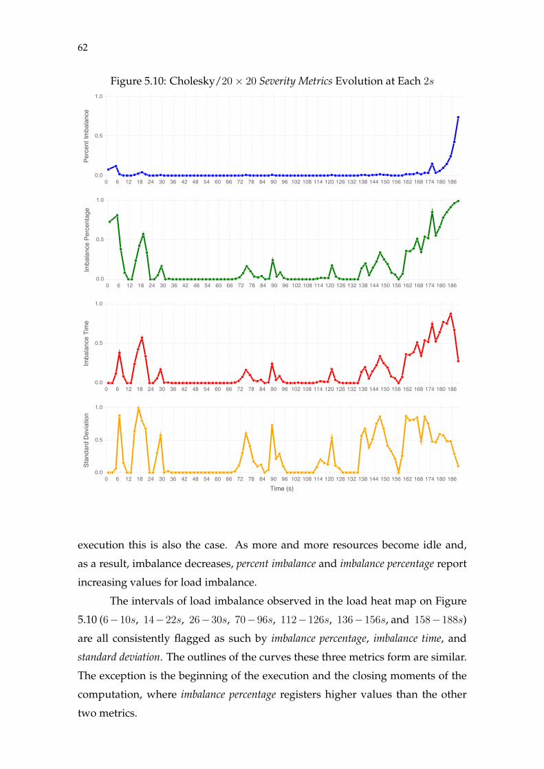
62

Figure 5.10: Cholesky/20× 20 Severity Metrics Evolution at Each 2s

��

� � ��

��

��

��

��

� � ��

��

��

��

��

� � ��

��

��

��

��

� � ��

��

��

��

execution this is also the case. As more and more resources become idle and,

as a result, imbalance decreases, percent imbalance and imbalance percentage report

increasing values for load imbalance.

The intervals of load imbalance observed in the load heat map on Figure

5.10 (6−10s, 14−22s, 26−30s, 70−96s, 112−126s, 136−156s, and 158−188s)

are all consistently flagged as such by imbalance percentage, imbalance time, and

standard deviation. The outlines of the curves these three metrics form are similar.

The exception is the beginning of the execution and the closing moments of the

computation, where imbalance percentage registers higher values than the other

two metrics.

63

Percent imbalance, imbalance percentage, imbalance time, and standard deviation

disagree in which interval execution is most imbalanced. For the first three met-

rics, the end of the execution, after the 180s mark, register the most severe load

dispersion. Load imbalance as measured by standard deviation, however, is at its

peak during the 12− 24s span.


The evolution of both load distribution shape metrics under analysis is

depicted in Figure 5.11. The time step length employed to determine the progress

of workload distribution is 2s, conforming with Figure 5.9.

Figure 5.11: Cholesky/20× 20 Shape Metrics Evolution at Each 2s

��

� � ��

�

��

��

��

� � ��

��

��

�

�

�

��

For most of the execution, skewness is negative and, hence, load distribu-

tion is predominantly right-skewed. This occurs both in intervals of the execution

where load is completely balanced and in which load is dispersed. The stretch

of time spanning from 30s to 70s, for instance, is one where load is balanced and

resources are fully occupied. Load skewness yields negative results for the ma-

jority of this period. Even more troubling is the fact that some of these perfectly

balanced spans of time (e.g. 36− 40s, 48− 50s) produce the lowest levels of load

skewness.

Load kurtosis, for most of the time, assumes values close to zero. This situ-

ation arises both in periods where load is perfectly balanced, as in, for example,

the 10 − 14s stretch, and in periods where load distribution is uneven such as

64

the interval starting at 160s and going all the way until the end of period under

consideration. The highest kurtosis value held for the execution’s load distribu-

tion is close to 30 and it occurs exclusively at moments in which load is perfectly

balanced, such as the 36− 40s interval.

Discussion

The massive increase registered by percent imbalance at the end of execution

exposes the difficulties imposed by the wide scale of values the metric assumes.

Mapping different degrees of load imbalance to such disparate values compli-

cates the evaluation proposed in this dissertation. Furthermore, the normalized

value of approximately 0.75 registered at the end of execution is a departure from

the behavior for percent imbalance seen in the Ondes3D runs analyzed in Section

5.2.1.

The highest value registered for the metric in these executions was 0.07.

Hence, according to the measure load imbalance is more than 10× worse in the

closing moments of this Cholesky decomposition execution than it ever was in the

two simulator runs examined earlier. The load distribution in which this value

of percent imbalance was seen consists in 30 resources being completely idle, one

resource registering 0.25 normalized load and another, 0.75.

Imbalance percentage also registers a significant increase in the final seconds

of the computation. For these measures, there is a clear correlation between idle-

ness and the value yielded by the metric. Time steps in which resources register

0.0 normalized load are the ones for which both measures present the highest

values. The intervals 0 − 6s and 14 − 22s are examples of circumstances where

this pattern can be detected. This behavior had been in display before, but it be-

comes more evident in this execution, which exhibits load patterns that are more

intricate than the ones seen previously.

5.2.2.2 80× 80 Blocks

The second run of StarPU’s Cholesky decomposition performed on a 20000×

20000 single precision floating point matrix differs from the previous execution in

the size of the blocks into which the input was decomposed. Instead of splitting

the input into 20 × 20 blocks, for this run input was decomposed into 80 × 80

65

blocks. The different choice for the size of the blocks into which the input is par-

titioned led to significantly better performance. The computation was complete

in 42.8s or, approximately, 22% of the previous execution run time.

Figure 5.12 illustrates the progression of normalized load for every re-

source during the execution of the application. For this specific run, as was

the case with the Ondes3D executions, a 1s time step was employed in order to

present the progress of load per resource at an adequate level of detail.

Figure 5.12: Cholesky/80× 80 Normalized Load Evolution at Each 1s

��

� � � � � � � � � � ��

��

��

��

��

��

��

Load Analysis

The image informs that load distribution evolves in 4 distinct phases. Af-

ter an initial 5s period where resources are completely idle, computation starts

across all resources. The 1s interval between 5s and 6s yields a normalized load

slightly higher than zero for all cores. From this point onwards, until 42s into exe-

cution, resources register full occupation. There are only a few 1s non-contiguous

stretches where a few of the resources yield normalized load modestly below 1.0.

These occur in the time steps starting 18s, 29s, 32s, 35s, 39s, and 41s into execu-

tion.

In the fourth and last stage of this Cholesky decomposition computation,

represented by the last time slice of Figure 5.12, normalized loads for all re-

sources decrease. The reduction in computational load within this final second

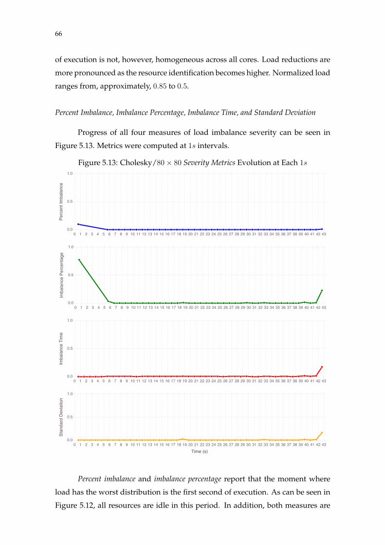
66

of execution is not, however, homogeneous across all cores. Load reductions are

more pronounced as the resource identification becomes higher. Normalized load

ranges from, approximately, 0.85 to 0.5.


Progress of all four measures of load imbalance severity can be seen in

Figure 5.13. Metrics were computed at 1s intervals.

Figure 5.13: Cholesky/80× 80 Severity Metrics Evolution at Each 1s

��

� � � � � � � � � � ��

��

��

��

��

� � � � � � � � � � ��

��

��

��

��

� � � � � � � � � � ��

��

��

��

��

� � � � � � � � � � ��

��

��

��

Percent imbalance and imbalance percentage report that the moment where

load has the worst distribution is the first second of execution. As can be seen in

Figure 5.12, all resources are idle in this period. In addition, both measures are

67

undefined in the period between 1 and 5s, as the absence of points drawn on top

of the line implies. Imbalance time and standard deviation, on the other hand, report

this 5s period as having inexistent load imbalance.

For the remainder of the execution load imbalance gauged by percent imbal-

ance, imbalance percentage, imbalance time, standard deviation yields zero or near zero

values, reporting the almost nonexistent load imbalance between resources. In

the non-contiguous time slices where normalized load for a few of the resources

stray modestly from full occupation, a slight increase can be observed in imbalance

percentage, imbalance time, and standard deviation.

Even in these small intervals where load imbalance increases, it only does

so by an almost insignificant amount, which is appropriate given that the imbal-

ance is barely noticeable in Figure 5.13. In the closing second of the computation,

the period in which load imbalance is most clear, all four metrics register an in-

crease.


Load distribution shape measures evolution for the Cholesky decomposi-

tion execution under consideration is shown in Figure 5.14.

Figure 5.14: Cholesky/80× 80 Shape Metrics Evolution at Each 1s

��

� � � � � � � � � � ��

�

�

��

��

� � � � � � � � � � ��

��

�

�

��

As was the case with percent imbalance and imbalance percentage, skewness

and kurtosis are undefined in the 1 − 5s interval. The plot reveals a more diverse

behavior for load skewness than the one revealed by load distribution. Skewness is

68

mostly negative in the first 25s of execution, denoting that the bulk of resources

loads are above the average. Afterwards, load skewness moves closer to zero,

oscillating between negative and slightly positive values.

Kurtosis lingers around zero for most of the execution, yielding both posi-

tive and negative values. Within the period of the computation where resources

register some activity (5 − 42s), there are stretches where kurtosis indicates that

load distribution is severely leptokurtic, suggesting that the dispersion registered

within these time frames, however small, is mostly explained by outliers. While

kurtosis does yield negative values as well, the are small in magnitude.

Discussion

The recurrent situation of both percent imbalance and imbalance percentage

recording their highest values of load imbalance during time steps where re-

sources are nearly all idle demands further investigation. Percent imbalance is

defined as a measure of the potential performance gains a perfectly balanced load

would yield (PEARCE et al., 2012). Similarly, imbalance percentage quantifies the

percentage of time all resources, excluding the processing element with highest

computational load, are not performing useful work (DEROSE; HOMER; JOHN-

SON, 2007).

Hence, both metrics take into account not only the disparities in computa-

tional load among resources, but the idleness that could potentially be exploited

through increased parallelism. This is the reason why in scenarios where loads

are similar across all resources, but resources are mostly idle, both measures yield

values close to or at the highest possible levels they can achieve.

Another issue regarding percent imbalance and imbalance percentage revealed

in the analysis of load imbalance throughout this execution is that both measures

can be undefined for certain time frames. In order to properly address this cir-

cumstance, the mathematical definition of each metric is reconsidered. First, per-

cent imbalance (λ) is computed through the following expression.

λ = (Lmax

L− 1)× 100 (5.1)

Hence, for percent imbalance, a situation where all resources are completely

idle would yield an average load of 0s and, as a result, would cause a division

69

by zero to be performed when computing the metric. Consequently, in such sit-

uations, percent imbalance is undefined. The formula that calculates imbalance per-

centage (I%) for a given load distribution and a certain number of resources (n) is

presented below.

I% =Lmax − L

Lmax

× n

n− 1(5.2)

Therefore, for the same load distribution pattern where no activity is reg-

istered in any resource, imbalance percentage would be undefined as well, since

the maximum load registered would be 0s and, once more, a division by zero is

required to calculate the measure. And this is the scenario recorded in the 1− 5s

interval. Since all resources yield 0.0 normalized load, both measures could not

be computed for this time span.

This represents another aspect of percent imbalance and imbalance percentage

that cannot be overlooked, for both practical and theoretical reasons. Most pro-

gramming languages throw an exception when a division by zero is executed.

Hence, any load balancer relying on one of these measures of load imbalance

ought to be aware of such situation so that it can be properly handled. Moreover,

in theory, one would expect a metric that quantifies load imbalance severity to

produce real values for all possible load distributions an application might yield.

Within the same period of time, skewness and kurtosis are also undefined.

Both measures require that resource computational loads register some disper-

sion, independent of how small this difference between resource computational

loads is, to be properly computed. Zero variation leads to illegal divisions in both

these statistical moments computations.

Hence, while percent imbalance and imbalance percentage do not yield a real

value when no activity is registered in any resource, skewness and kurtosis are not

defined whenever all resources register the same computational load, irrespective

of the load level resources yield. Standard deviation and imbalance time, on the

other hand, are always defined regardless of how load is distributed.

Both Cholesky decomposition executions were representative examples of

the distinct purposes the two sets of metrics studied in this document serve as

load distribution measures. The overall behavior for skewness and kurtosis when

compared to the behavior registered for the load imbalance severity measures,

as suggested by the outline of their curves, is evidence of this. Variations in load

70

imbalance as gauged by percent imbalance, imbalance percentage, imbalance time, and

standard deviation do not translate into oscillations in skewness and kurtosis.

5.3 Summary

The analysis of load distribution metrics performed in Section 5.2 revealed

aspects regarding how these measures quantify load imbalances in parallel ap-

plications. Since the four executions used as case studies possessed different pat-

terns of load distribution, a comprehensive set of scenarios was available for the

measures to be thoroughly evaluated.

The Ondes3D execution where synchronous communication was used (Fig-

ure 5.3) boasted for most of the computation relative load balance. Yet, although

load levels were similar, most resources recorded computational loads at the mid-

dle of the scale within these periods. In addition, the execution presented a period

where a few resources yielded loads that where clear outliers when compared to

the rest of the processor cores.

Throughout most of the following Ondes3D execution (Figure 5.6), all re-

sources yielded computational loads at the upper end of the scale. However,

loads were never completely balanced and, as a result, some dispersion was al-

ways present. The first of the two Cholesky decomposition executions (Figure

5.9) was unique because it recorded very diverse load distribution patterns with

several different situations of load imbalance interspersed within periods of full

occupation in all resources.

The second Cholesky decomposition run (Figure 5.12), on the other hand,

displayed a synchronized load distribution with resources starting to compute at

the exact same time and maintaining a near perfect load balance until computa-

tion completed. Moreover, all executions included periods of complete or near

complete idleness across all resources, allowing the measures to be examined in

such situations as well. Hence, by revealing the response the measures presented

to numerous patterns of load distribution, a better grasp of each metric was ob-

tained.

The patterns uncovered in the analysis regarding the behavior of percent

imbalance, imbalance percentage, imbalance time, and standard deviation allowed for

the differences in how these metrics quantify load imbalance to be made clear.

71

Assuming that these measures, by quantifying the severity of load imbalance in

parallel applications, would agree on what exactly consists an imbalanced load

and in the magnitude that should be assigned to a given imbalance has been

shown to be inappropriate. These measures consider load imbalance severity in

different ways.

Since each metric has a different perspective, the analysis makes one won-

der what is a proper definition of load imbalance. The point of view given by

imbalance time and standard deviation measures difference in loads, regardless of

load levels. However, as has been demonstrated above, the former measure is

more prone to be affected by outliers, while the latter oscillates modestly in such

situations. Unlike the other three measures, standard deviation assigns higher val-

ues to diversity than to extremism.

Percent imbalance and imbalance percentage, on the other hand, when com-

puting the level of imbalance a particular load distribution has, consider the

available unused computing power and not only the disparities in load levels

across resources. Yet, each of these metrics assesses imbalance differently.

Percent imbalance measures the performance lost to imbalanced load or,

conversely, the performance that could be reclaimed by balancing the load, while

imbalance percentage corresponds to the percentage of time resources, excluding

the most loaded, are idling. Nonetheless, both establish a correlation between

idleness and the value yielded for the particular measure. This strays from the

common sense view that load imbalance is simply the unevenness in load levels

between resources.

The differences in how each of the four severity measures account for load

imbalance are represented in Figure 5.15. Red bars represent the load each re-

source yielded during a given time span, while the blue bars represent the time

each resource was idle. Hence, the image communicates that while imbalance time

and standard deviation consider only the load while determining the degree of

load imbalance severity, percent imbalance and imbalance percentage consider both

the load levels and the idle computing power that has been wasted.

Given all the evidence and information, it is possible to define a position

regarding the severity measures examined above. Since both percent imbalance

and imbalance percentage take into account not only the differences in computa-

tional load between resources but also the wasted computational power, these

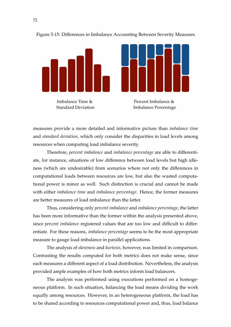
72

Figure 5.15: Differences in Imbalance Accounting Between Severity Measures

Imbalance Time & Standard Deviation

Percent Imbalance & Imbalance Percentage

measures provide a more detailed and informative picture than imbalance time

and standard deviation, which only consider the disparities in load levels among

resources when computing load imbalance severity.

Therefore, percent imbalance and imbalance percentage are able to differenti-

ate, for instance, situations of low difference between load levels but high idle-

ness (which are undesirable) from scenarios where not only the differences in

computational loads between resources are low, but also the wasted computa-

tional power is minor as well. Such distinction is crucial and cannot be made

with either imbalance time and imbalance percentage. Hence, the former measures

are better measures of load imbalance than the latter.

Thus, considering only percent imbalance and imbalance percentage, the latter

has been more informative than the former within the analysis presented above,

since percent imbalance registered values that are too low and difficult to differ-

entiate. For these reasons, imbalance percentage seems to be the most appropriate

measure to gauge load imbalance in parallel applications.

The analysis of skewness and kurtosis, however, was limited in comparison.

Contrasting the results computed for both metrics does not make sense, since

each measures a different aspect of a load distribution. Nevertheless, the analysis

provided ample examples of how both metrics inform load balancers.

The analysis was performed using executions performed on a homoge-

neous platform. In such situation, balancing the load means dividing the work

equally among resources. However, in an heterogeneous platform, the load has

to be shared according to resources computational power and, thus, load balance

73

gains a new meaning.

Therefore, the methodology used in the analysis presented above would

not be appropriated. Since load is measured in seconds, the assumption that

resources should register similar workload would not be valid, because one unit

of time of computation in different resources cannot be considered equivalent if

these resources possess different computing power. Additionally, the measures

examined here are not appropriate to gauge load distributions in heterogeneous

environments. However, metrics to properly quantify load distributions in such

scenarios exist (YANG et al., 2003).

74

6 CONCLUSION

This dissertation presented a study demonstrating the means by which

different load distribution metrics inform the dynamic patterns of load allocation

in high-performance applications executed in an homogeneous multiprocessing

platform. Metrics quantifying aspects of load distribution are an important part

of the process of load balancing, which in itself is critical for the proper perfor-

mance of parallel codes.

The goal of the study was to establish the degree to which measures em-

ployed to gauge load distribution are informative in characterizing the patterns

of work allocation in parallel applications. The load distribution metrics exam-

ined were percent imbalance, imbalance percentage, imbalance time, standard deviation,

skewness, and kurtosis. Through the examination performed, the metrics similar-

ities and particularities were revealed. This knowledge allows for a better grasp

of the measures and, therefore, is valuable for load balancers developers.

Two applications were employed as case studies. Ondes3D, a seismic wave

propagation simulator that uses MPI as its parallelization support and an applica-

tion, written with the StarPU task programming library, that computes a Cholesky

decomposition. These provided with multiple load distribution scenarios, allow-

ing for the measures to be evaluated exhaustively.

The methodology employed to perform the analysis of measures involved

first understanding how load distribution unraveled during a parallel applica-

tion execution and, afterwards, considering how each metric communicates such

progress. The notion of progress is given by dividing the application run in in-

tervals of identical length. For each interval, both the load distribution and the

behavior of each measure is determined.

The progress of load distribution for an execution is revealed with the as-

sistance of a heat map, while measures are depicted by simple line plots that es-

tablish the sequence of values each of them yielded. This two step process com-

bining analysis of load patterns and the measures constituted the process used

in the evaluation. The methodology, thus, was based on visual analysis of load

distribution evolution and the measures description of this evolution.

The results concerning percent imbalance, imbalance percentage, imbalance time,

and standard deviation made the differences in how these measures quantify load

75

imbalance explicit. While imbalance time and standard deviation oscillate entirely

according to disparities in loads between resources, percent imbalance and imbal-

ance percentage are also affected by idleness. Hence, given that it provided a more

complete view of load distribution and, also, it mapped scenarios of load distri-

bution to values more coherently than percent imbalance, imbalance percentage was

found to be the most appropriate measure of load imbalance severity.

For skewness and kurtosis, the second set of metrics investigated, the broad

spectrum of load distribution scenarios allowed for these obscure measures to be

exposed and, thus, further understood in how each informs load balancers.

Parallel systems are increasingly heterogeneous in regards to the process-

ing elements composing them. Graphical processing units (KINDRATENKO

et al., 2009) and co-processors (DONGARRA et al., 2015) are gaining popular-

ity, and are now used along with traditional central processing units to compute

high-performance applications. Load balance acquires a distinct meaning in such

environments since another variable - i.e. the computing power each resource

possesses - must be considered when distributing tasks. Hence, given the current

relevance these systems have, one direction to explore in future work is the eval-

uation of measures appropriate for heterogeneous environments (YANG et al.,

2003).

76

REFERENCES

ARZUAGA, E.; KAELI, D. R. Quantifying Load Imbalance on VirtualizedEnterprise Servers. In: Proceedings of the First Joint WOSP/SIPEWInternational Conference on Performance Engineering. New York, NY, USA:ACM, 2010. (WOSP/SIPEW ’10), p. 235–242.

AUGONNET, C. et al. StarPU: A Unified Platform for Task Schedulingon Heterogeneous Multicore Architectures. In: Proceedings of the 15thInternational Euro-Par Conference. Berlin, Germany: Springer BerlinHeidelberg, 2009. p. 863–874.

BERGER, M. J.; OLIGER, J. Adaptive Mesh Refinement for Hyperbolic PartialDifferential Equations. Journal of Computational Physics, v. 53, n. 3, p. 484–512,1984.

BOHME, D. et al. Scalable Critical-Path Based Performance Analysis. In:Proceedings of the 26th International Parallel Distributed ProcessingSymposium. Piscataway, NJ, USA: IEEE, 2012. (IPDPS ’2012), p. 1330–1340.

BONETI, C. et al. A Dynamic Scheduler for Balancing HPC Applications.In: Proceedings of the 2008 ACM/IEEE Conference on Supercomputing.Piscataway, NJ, USA: IEEE, 2008. (SC ’08), p. 41:1–41:12.

DEROSE, L.; HOMER, B.; JOHNSON, D. Detecting Application Load Imbalanceon High End Massively Parallel Systems. In: Proceedings of the 13thInternational Euro-Par Conference. Berlin, GER: Springer Berlin Heidelberg,2007. p. 150–159.

DONGARRA, J. et al. HPC Programming on Intel Many-integrated-coreHardware with MAGMA Port to Xeon Phi. Scientific Programming, HindawiPublishing Corp., New York, NY, United States, v. 2015, p. 9:9–9:9, Jan. 2015.

DROR, R. O. et al. Biomolecular Simulation: A Computational Microscope forMolecular Biology. Annual Review of Biophysics, v. 41, n. 1, p. 429–452, 2012.

DUPROS, F. et al. Exploiting Intensive Multithreading for the Efficient Simulationof 3D Seismic Wave Propagation. In: Proceedings of the 11th IEEE InternationalConference on Computational Science and Engineering. Piscataway, NJ, USA:IEEE, 2008. (CSE ’08), p. 253–260.

ELIAS, R. N.; COUTINHO, A. L. G. A. Stabilized Edge-based Finite ElementSimulation of Free-surface Flows. International Journal for Numerical Methodsin Fluids, John Wiley & Sons, Ltd., v. 54, n. 6-8, p. 965–993, 2007.

FATICA, M.; PHILLIPS, E. Pricing American Options with Least Squares MonteCarlo on GPUs. In: Proceedings of the 6th Workshop on High PerformanceComputational Finance. New York, NY, USA: ACM, 2013. (WHPCF ’13), p.5:1–5:6.

77

FEO, J. et al. Irregular Applications: Architectures & Algorithms. In: Proceedingsof the 1st Workshop on Irregular Applications: Architectures and Algorithms.New York, NY, USA: ACM, 2011. (IA3 ’11), p. 1–2.

GRAMA, A. et al. Introduction to Parallel Computing. 2nd. ed. Boston, MA,USA: Addison-Wesley, 2003.

HEY, A. J. G.; TANSLEY, S.; TOLLE, K. M. The Fourth Paradigm: Data-IntensiveScientific Discovery. Redmond, WA, USA: Microsoft Research, 2009.

KINDRATENKO, V. V. et al. GPU Clusters for High-performance Computing. In:Proceedings of the 2009 IEEE International Conference on Cluster Computingand Workshops. Piscataway, NJ, USA: IEEE, 2009. p. 1–8.

LIGOWSKI, L.; RUDNICKI, W. An Efficient Implementation of Smith-WatermanAlgorithm on GPU using CUDA, for Massively Parallel Scanning of SequenceDatabases. In: Parallel Distributed Processing, 2009. IPDPS 2009. IEEEInternational Symposium on. Piscataway, NJ, USA: IEEE, 2009. p. 1–8.

MICHALAKES, J.; VACHHARAJANI, M. GPU Acceleration of NumericalWeather Prediction. Parallel Processing Letters, v. 18, n. 04, p. 531–548, 2008.

MOCZO, P.; ROBERTSSON, J. O.; EISNER, L. The Finite-Difference Time-Domain Method for Modeling of Seismic Wave Propagation. In: Advances inWave Propagation in Heterogenous Earth. Amsterdam, Netherlands: Elsevier,2007, (Advances in Geophysics, v. 48). p. 421– 516.

PAGÈS, G.; WILBERTZ, B. GPGPUs in Computational Finance: Massive ParallelComputing for American Style Options. Concurrency and Computation:Practice and Experience, John Wiley & Sons, v. 24, n. 8, p. 837–848, 2012.

PEARCE, O. et al. Quantifying the Effectiveness of Load Balance Algorithms. In:Proceedings of the 26th ACM International Conference on Supercomputing.New York, NY, USA: ACM, 2012. (ICS ’12), p. 185–194.

QUIRINO, T. S.; DELGADO, J.; ZHANG, X. Improving the Scalability ofa Hurricane Forecast System in Mixed-Parallel Environments. In: HighPerformance Computing and Communications, 2014 IEEE 6th Intl Sympon Cyberspace Safety and Security, 2014 IEEE 11th Intl Conf on EmbeddedSoftware and Syst (HPCC,CSS,ICESS), 2014 IEEE Intl Conf on. Piscataway, NJ,USA: IEEE, 2014. p. 276–281.

REED, D. A. et al. Computational Science: Ensuring America’s Competitive-ness. Arlington, VA, USA, 2005. President’s Information Technology AdvisoryCommitee.

TALLENT, N. R.; ADHIANTO, L.; MELLOR-CRUMMEY, J. M. ScalableIdentification of Load Imbalance in Parallel Executions Using Call Path Profiles.In: Proceedings of the 2010 ACM/IEEE International Conference for HighPerformance Computing, Networking, Storage and Analysis. Washington, DC,USA: IEEE Computer Society, 2010. (SC ’10), p. 1–11.

78

TAYLOR, R. G. Models of Computation and Formal Languages. Oxford, UK:Oxford University Press, 1998.

TESSER, R. K. et al. Improving the Performance of Seismic Wave Simulationswith Dynamic Load Balancing. In: Proceedings of the 22nd EuromicroInternational Conference on Parallel, Distributed, and Network-BasedProcessing. Piscataway, NJ, USA: IEEE, 2014. p. 196–203.

ULLMAN, J. D. NP-complete Scheduling Problems. Journal of Computer andSystem Sciences, Academic Press, Inc., Orlando, FL, USA, v. 10, n. 3, p. 384–393,Jun. 1975.

XU, Z.; HUANG, R.; BHUYAN, L. N. Load Balancing of DNS-based DistributedWeb Server Systems with Page Caching. In: Proceedings of the 10thInternational Conference on Parallel and Distributed Systems. Piscataway, NJ,USA: IEEE, 2004. (ICPADS ’2004), p. 587–594.

YANG, X. et al. A General Metric of Load Balancing in δ-Range. In: AdvancedParallel Processing Technologies: Proceedings of the 5th InternationalWorkshop. Berlin, Germany: Springer Berlin Heidelberg, 2003. (APPT ’2003), p.311–321.

YELICK, K. A. Programming Models for Irregular Applications. SIGPLANNotices, ACM, New York, NY, USA, v. 28, n. 1, p. 28–31, 1993.

79

APPENDIX A — ESTUDOS DE MEDIDAS DE DISTRIBUIÇÃO DE CARGA

PARA APLICAÇÕES DE ALTO DESEMPENHO

A.1 Introdução

Computação de alta desempenho consiste no uso de conceitos de proces-

samento paralelo para a execução de aplicações que consumiriam uma enorme

quantidade de tempo caso fossem computadas de maneira sequencial. Em out-

ras palavras, computação de alto desempenho trata do acúmulo de poder de

processamento de forma a disponibilizar desempenho computacional que seria

inatingível em um simples computador comum ou em um dispositivo móvel.

Consequentemente, problemas computacionais complexos que demandam bas-

tante memória, processamento e banda de rede para serem executados podem

ser computados em um período de tempo aceitável. O uso de sistemas de alto

desempenho ocorre em áreas diversas das ciências naturais (DROR et al., 2012)

(MICHALAKES; VACHHARAJANI, 2008), bem como em problemas de engen-

haria (ELIAS; COUTINHO, 2007) e economia (PAGÈS; WILBERTZ, 2012).

Computação de alto desempenho e computação paralela estão, portanto,

interligadas. Neste contexto, balanceamento de carga é essencial para aplicações

paralelas obterem o melhor desempenho possível. O custo de uma má distribuição

de carga aumenta conforme o sistema paralelo cresce em tamanho (BONETI et

al., 2008). Por essas razões, um balanceamento de carga adequado é fundamental

para aplicações paralelas de larga escala.

Porém, em aplicações paralelas ditas irregulares, a carga computacional

apresenta um comportamento dinâmico. Tal situação induz disparidades nas car-

gas computacionais dos recursos participantes da computação. Por consequên-

cia, uma redistribuição recorrente da carga entre os recursos é de extrema im-

portância para que se atinja o desempenho necessário para que problema de larga

escala sejam computados. Considerando que aplicações de alto desempenho ir-

regulares são cada vez mais comuns (FEO et al., 2011), o balanceamento dinâmico

de carga é vital para computação de alto desempenho atualmente.

Balanceamento de carga envolve medir o estado da distribuição de carga,

decidir como redistribuir esta carga e, por fim, realizar a realocação propria-

mente dita. Portanto, métricas que quantificam a distribuição de carga consistem

80

em uma importante faceta deste procedimento. Contudo, o processo de redis-

tribuição de carga computacional entre recursos gera um overhead que pode im-

pactar o desempenho da aplicação negativamente, caso seja realizado sem neces-

sidade. Adicionalmente, o adiamento da redistribuição também pode gerar um

impacto indesejado sobre o tempo de execução da aplicação. Por estas razões,

estas métricas de distribuição de carga em aplicações paralelas devem ser com-

pletamente compreendidas para que possam ser interpretadas corretamente e,

desta forma, guiar o balanceamento de carga de maneira efetiva.

Como resultado desta conjuntura, medidas comumente utilizadas como

indicadores de distribuição de carga em aplicações de alto desempenho foram ex-

aminados neste estudo. Considerando o aspecto dinâmico e recorrente presente

no processo de balanceamento de carga, a investigação examina como estas me-

didas quantificam a distribuição de carga em intervalos regulares durante a exe-

cução da aplicação paralela, ao invés de simplesmente considerar um agregado

que inclua a computação completa. Em outras palavras, conforme a computação

progride, as medidas são computadas para determinar como estas comunicam a

evolução da distribuição de carga.

Seis métricas foram avaliadas: percent imbalance, imbalance percentage, im-

balance time, desvio padrão, skewness e kurtosis. A expectativa é de que a análise

revele as virtudes e deficiências que cada uma destas métricas possui, bem como

as diferenças presentes na maneira como descrevem o progresso no tempo da

distribuição de carga em aplicações paralelas. Até onde sabemos, a investigação

proposta neste documento não foi realizada ainda.

A.2 Metodologia

A investigação envolverá examinar como cada uma das métricas quan-

tifica o desdobramento da distribuição de carga em algumas execuções de apli-

cações paralelas. Se espera que esse procedimento forneça um entendimento das

virtudes e falhas das medidas selecionadas.

81

A.2.1 Análise de Carga

A carga computacional total de um recurso é computada através do so-

matório da duração, medida em segundos, de todas operações classificadas como

carga computacional executados pelo recurso durante a computação em questão.

A evolução da distribuição é percebida através da divisão da execução em inter-

valos de tamanho igual e na determinação dos padrões de distribuição para cada

um destes períodos separadamente.

A análise irá considerar a carga normalizada registrada por cada recurso

em todo o intervalo no qual a execução foi divida. A carga normalizada de um

recurso para um determinado período de tempo consiste na razão entre a carga

computacional deste recurso e a duração do período. A quantidade é, portanto,

adimensional e representa a fração de tempo que um recurso estava ocupado.

Carga computacional normalizada estará, logo, sempre entre 0 e 1, sendo 0 a

ausência da carga, 1 caso contrário.

O progresso da distribuição de carga para uma execução é analisado atráves

de uma representação gráfica chamada de mapa de calor. Em tal representação,

valores são representados como cores. Portanto, a análise dos padrões de dis-

tribuição de carga de uma execução de aplicação paralela consiste em obser-

var um mapa de calor representando a evolução desta distribuição no tempo.

A Figura A.1 demonstra como o progresso da distribuição de carga é analisado

nesta dissertação.

A imagem representa a evolução da carga normalizada para todo recurso

que participou da computação. A representação considerada engloba a execução

completa da aplicação. O eixo horizontal representa a progressão do tempo do

momento em que a computação iniciou ao momento em que foi encerrada. A

progressão do tempo é sempre apresentada em segundos. No caso da execução

representada na Figura A.1, a computação durou aproximadamente 78s. Para

permitir que a evolução da distribuição de carga pudesse ser percebida, a exe-

cução foi dividida em intervalos de 1s.

A extensão da duração dos intervalos através dos quais o progresso da exe-

cução de uma aplicação é percebido é escolhida de maneira empírica. O processo

de selecionar o tamanho dos intervalos envolve dois aspectos. Primeiro, para

uma dada execução, o intervalo deve ser grande o suficiente para que a repre-

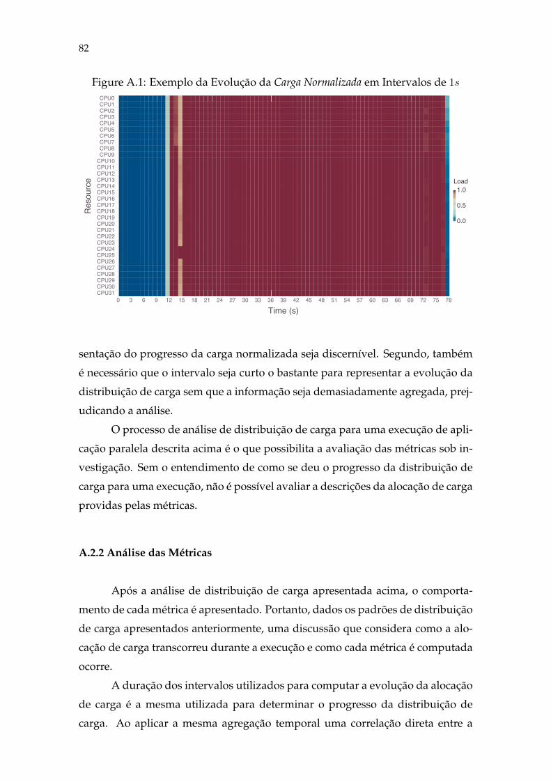
82

Figure A.1: Exemplo da Evolução da Carga Normalizada em Intervalos de 1s

��

� � � � ��

��

��

��

��

��

��

sentação do progresso da carga normalizada seja discernível. Segundo, também

é necessário que o intervalo seja curto o bastante para representar a evolução da

distribuição de carga sem que a informação seja demasiadamente agregada, prej-

udicando a análise.

O processo de análise de distribuição de carga para uma execução de apli-

cação paralela descrita acima é o que possibilita a avaliação das métricas sob in-

vestigação. Sem o entendimento de como se deu o progresso da distribuição de

carga para uma execução, não é possível avaliar a descrições da alocação de carga

providas pelas métricas.

A.2.2 Análise das Métricas

Após a análise de distribuição de carga apresentada acima, o comporta-

mento de cada métrica é apresentado. Portanto, dados os padrões de distribuição

de carga apresentados anteriormente, uma discussão que considera como a alo-

cação de carga transcorreu durante a execução e como cada métrica é computada

ocorre.

A duração dos intervalos utilizados para computar a evolução da alocação

de carga é a mesma utilizada para determinar o progresso da distribuição de

carga. Ao aplicar a mesma agregação temporal uma correlação direta entre a

83

análise de carga e as métricas pode ser estabelecida. O propósito é determinar se

as medidas comunicam o mesmo comportamento evolucionário desvendado na

análise precedente.

Com o intuito de ilustrar como a evolução das medidas de balanceamento

de carga são representadas, a Figura A.2 apresenta a evolução de cada uma das

seis medidas investigadas. Da mesma forma como na análise de carga presente

na Figura A.1, a duração dos intervalos é de 1s. O eixo horizontal representa

a passagem do tempo em segundos, enquanto que o vertical contém o espectro

de valores assumidos pela medida. Pontos indicam o valor registrado pela me-

dida em um determinado intervalo. Uma linha conecta estes pontos na ordem

temporal com o objetivo de prover um senso da progressão da métrica no tempo.

Considerando que, com base no aspecto da distribuição de carga quantifi-

cado, as medidas sob análise podem ser separadas em dois grupos. A análise é

realizada em separado para cada grupo. Primeiramente as métricas que medem

a severidade do desbalanceamento de carga são examinadas. Este grupo é com-

posto por percent imbalance, imbalance percentage, imbalance time e desvio padrão. Em

seguida, as métricas que quantificam a forma da distribuição de carga, skewness e

kurtosis, são investigadas.

As medidas de severidade são normalizadas para que estejam em uma

escala comum e, consequentemente, torne a comparação entre as mesmas mais

simples e direta. Assim, para cada uma destas medidas, o valor registrado em

cada intervalo é ajustado para que fique entre 0 e 1. Para isto, o valor da métrica

é dividido pelo valor máximo atingível pela medida. Dado que tanto skewness

como kurtosis podem registrar valores negativos e positivos, os valores obtidos

para cada uma destas medidas não foram normalizados, visto que isto incorreria

em perda de informação valiosa a respeito da distribuição de carga.

A combinação da análise da distribuição de carga, descrita na seção an-

terior, e da análise das medidas de balanceamento de carga , detalhada acima,

constitui a metodologia aplicada para a avaliação das métricas selecionadas neste

estudo. Ambos componentes desta metodologia dependem da análise visual de

imagens representando a distribuição de carga e a descrição que as métricas apre-

sentam desta distribuição. A associação entre os padrões apresentados por cada

imagem permite que as vantagens, desvantagens e diferenças entre medidas se-

jam expostas.

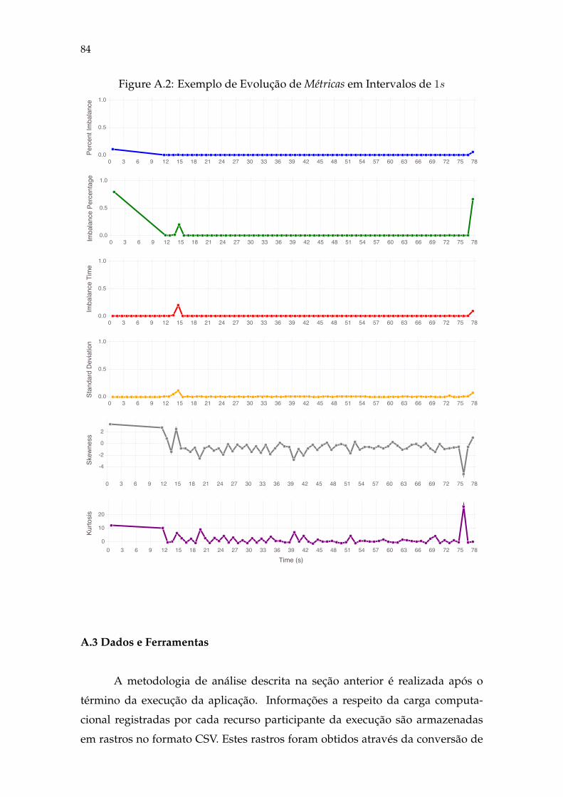
84

Figure A.2: Exemplo de Evolução de Métricas em Intervalos de 1s

��

� � � � ��

�

��

��

��

� � � � ��

��

��

�

�

��

� � � � ��

��

��

��

��

� � � � ��

��

��

��

��

� � � � ��

��

��

��

��

� � � � ��

��

��

��

A.3 Dados e Ferramentas

A metodologia de análise descrita na seção anterior é realizada após o

término da execução da aplicação. Informações a respeito da carga computa-

cional registradas por cada recurso participante da execução são armazenadas

em rastros no formato CSV. Estes rastros foram obtidos através da conversão de

85

arquivos no formato Pajé1 utilizando a ferramenta PajeNG2.

O pacote YAJP.jl3, desenvolvido utilizando a linguagem de programação

Julia4, foi empregado para gerar as imagens utilizadas no processo de análise das

métricas de distribuição de carga. Este pacote contém métodos para extrair e

analisar informações contidas em rastros de execução Pajé armazenados no for-

mato CSV.

Todos os rastros de execução utilizados neste estudo, bem como as ima-

gens representando os padrões de distribuição de carga e a evolução das medidas

para estas execuções são públicos5. O script usado para gerar os gráficos também

está presente neste repositório. O compilador para a linguagem Julia e o pacote

YAJP.jl são necessários para que este script possa ser executado com sucesso.

A.4 Resultados e Trabalhos Futuros

Duas aplicações foram utilizadas como estudos de caso. A primeira delas,

Ondes3D, consiste em um simulador de propagação de ondas sísmicas que utiliza

MPI como suporte para paralelização. A outra aplicação utilizada como estudo

de caso realiza uma operação de álgebra linear conhecida como decomposição

Cholesky. Esta aplicação foi desenvolvida com a biblioteca de programação orien-

tada a tarefas StarPU. Ambas aplicações proveram múltiplos e distintos cenários

de distribuição de carga, permitindo que as métricas fossem avaliadas. Todas

as execuções utilizadas neste trabalho foram realizadas em uma máquina ho-

mogênea multiprocessada.

Os resultados relacionados as medidas de severidade do desbalanceamento

de carga (i.e. percent imbalance, imbalance percentage, imbalance time e desvio padrão)

demonstraram as diferenças presentes na maneira como cada umas destas medi-

das quantifica a disparidade na distribuição de carga. Enquanto imbalance time e

desvio padrão oscilam inteiramente de acordo com diferenças presentes na carga

associada aos recursos, percent imbalance e imbalance percentage são afetados tam-

bém pela ociosidade registrada nos elementos computacionais. Logo, dado que

1http://paje.sourceforge.net/download/publication/lang-paje.pdf2https://github.com/schnorr/pajeng3https://github.com/flavioalles/YAJP.jl4http://julialang.org5https://github.com/flavioalles/data

86

propicia uma visão mais completa da distribuição de carga e, ainda, que mapeou

os diferentes cenários de distribuição apresentados nos estudos de caso de maneira

mais coerente se comparada a métrica percent imbalance, imbalance percentage foi

considerada a medida mais apropriada para medir a severidade do desbalancea-

mento de carga.

Contudo, a análise do segundo conjunto de métricas estudado foi limitada.

Contrastar os resultados obtidos por skewness e kurtosis não tem propósito, dado

que cada uma destas medidas quantifica um aspecto distinto da distribuição de

carga. Mesmo assim, a análise forneceu amplos exemplos de como cada uma

destas duas métricas informa o estado da distribuição de carga em uma aplicação

paralela.

Sistemas paralelos tem se tornado cada vez mais heterogêneos em relação

aos elementos de processamento que os compõem. Unidades de processamento

gráfico (KINDRATENKO et al., 2009) e coprocessadores (DONGARRA et al.,

2015) são utilizados em conjunto com unidades de processamento central em

máquinas de alto desempenho. Em ambientes heterogêneos como estes, bal-

anceamento de carga adquire um significado distinto, dado que outra variável

– i.e. o poder de computação que cada recurso possui – deve ser considerada

no momento da distribuição de tarefas. Portanto, como tais ambientes de com-

putação heterogênea tem ganho espaço na área de computação de alto desem-

penho, trabalhos futuros que avaliem medidas de distribuição de carga apropri-

ada para tal situação são uma possível via de exploração (YANG et al., 2003).

Documents

Study of Load Distribution Measures for High-performance