Embed Size (px)
Citation preview
Escola Tècnica Superior d'Enginyerires Industrial i Aeronàutica de Terrassa
UNIVERSITAT POLITÈCNICA DE CATALUNYA
Titulació:
Enginyeria Aeronàutica
Alumne:
Alejandro Roger Ull
Títol PFC:
STUDY OF MESH DEFORMATION FEATURES OF AN OPEN SOURCE
CFD PACKAGE AND APPLICATION TO A GEAR PUMP SIMULATION
Tutor del PFC:
Roberto Castilla López, David del Campo Sud.
Convocatòria de lliurament del PFC:
Juny 2012
Contingut d’aquest volum:
Memòria


Alejandro Roger Ull ETSEIAT 2012
License: This work is available under the terms of the Creative Commons
Attribution – NonCommercial – ShareAlike 3.0 Unported License (CC BY-NC-SA 3.0).
For more information please visit: http://creativecommons.org/licenses/by-nc-sa/3.0/
– 3 –
Alejandro Roger Ull ETSEIAT 2012
Keywords: Computational Fluid Dynamics, Dynamic Mesh, Gear Pump Simulation,
OpenFOAM.
Summary: A study of the mesh deformation capabilities of an open source
Computational Fluid Dynamics (CFD) package is presented in this document. First,
previous works on the matter are explained, and an introduction to dynamic meshes and
a description of OpenFOAM, the chosen CFD package, are presented. Second, the steps
needed to perform the two-dimensional simulation of an oil gear pump are developed in
detail. Those steps include meshing the geometry, moving the mesh and finally solving
the flow. The final part of this study includes the results and some conclusions, and
possible future and derived works are listed. At the end of the document the budget of
the study, environmental concerns and the bibliography and references are presented.
– 4 –
Alejandro Roger Ull ETSEIAT 2012
Table of Contents
1 Purpose......................................................................................................................11
2 Justification...............................................................................................................13
3 Scope..........................................................................................................................15
4 Introduction...............................................................................................................17
4.1 Previous Works...............................................................................................17
4.1.1 Analysis of External Gear Pumps...........................................................17
4.1.2 Initial Study of Mesh Deformation with OpenFOAM...........................19
4.2 Dynamic Mesh...............................................................................................19
4.3 OpenFOAM Description................................................................................21
4.3.1 Usage......................................................................................................21
4.3.2 Coding....................................................................................................22
4.3.3 Parallel Execution...................................................................................23
4.3.4 Dynamic Mesh Implementation.............................................................23
5 Development..............................................................................................................25
5.1 Initial Case Setup...........................................................................................25
5.2 Obtaining the Geometry.................................................................................26
5.3 Generating an STL File..................................................................................28
5.4 Meshing..........................................................................................................32
5.4.1 blockMesh..............................................................................................33
5.4.2 snappyHexMesh.....................................................................................35
5.4.3 decomposePar.........................................................................................38
5.4.4 extrudeMesh...........................................................................................40
5.4.5 runMesh..................................................................................................42
5.4.6 Improving the Meshing Procedure.........................................................44
5.5 Moving the Mesh...........................................................................................52
5.5.1 Creating a New Case Directory..............................................................52
5.5.2 Setting Up the Boundary Conditions......................................................53
5.5.3 Creating a User-Defined Boundary Condition.......................................59
5.5.4 Defining the Parameters of the Simulation............................................63
5.5.5 Running the Moving Gear......................................................................65
– 5 –
Alejandro Roger Ull ETSEIAT 2012
5.5.6 runMove.................................................................................................68
5.5.7 Testing the Limits of the Mesh...............................................................69
5.6 Performing a Complete Gearing Cycle..........................................................71
5.6.1 runAllMesh.............................................................................................72
5.6.2 runAllMove............................................................................................75
5.6.3 runPimple & runAllPimple.....................................................................77
6 Results and Conclusions...........................................................................................85
6.1 Results of This Study.....................................................................................85
6.2 Conclusions and Other Considerations..........................................................87
6.3 Future Work....................................................................................................89
7 Budget........................................................................................................................91
7.1 Work Hours....................................................................................................91
7.2 Hardware Infrastructure.................................................................................91
7.3 Software Licenses..........................................................................................92
7.4 Total................................................................................................................92
8 Environmental Effects..............................................................................................93
9 References..................................................................................................................95
– 6 –
Alejandro Roger Ull ETSEIAT 2012
List of Figures
Figure 4.1: Working principle of the external gear pump................................................17
Figure 4.2: Oil gear pump studied by David del Campo Sud in [1]................................18
Figure 4.3: File system of the cavity tutorial...................................................................21
Figure 5.1: Geometry of the gear pump..........................................................................26
Figure 5.2: File system of the gearFluent case................................................................26
Figure 5.3: Selection of patches in ParaView..................................................................27
Figure 5.4: STL file displayed in ParaView.....................................................................32
Figure 5.5: File system of the points2stl case..................................................................32
Figure 5.6: File system of the gearSnappy case..............................................................33
Figure 5.7: Broken mesh due to a low refinement (left) and correct mesh (right)..........37
Figure 5.8: File system of the gearExtrude case..............................................................40
Figure 5.9: The mesh boundary is badly messed after the extrusion...............................44
Figure 5.10: Detail of the mesh.......................................................................................44
Figure 5.11: The mesh improves greatly when using flattenMesh..................................46
Figure 5.12: Detail of the mesh.......................................................................................46
Figure 5.13: Errors on some faces that are out of place..................................................47
Figure 5.14: File system of the gearSnappy and gearExtrude cases...............................49
Figure 5.15: Mesh correctly generated with the final runMesh script.............................50
Figure 5.16: Mesh correctly generated. Detail of the gear meshing zone.......................51
Figure 5.17: Mesh correctly generated. Detail of the casing zone..................................51
Figure 5.18: File system of the gearMove case...............................................................52
Figure 5.19: Files required to create a user-defined boundary condition........................60
Figure 5.20: Modified cavity case for testing the user-defined boundary condition.......63
Figure 5.21: Deformation of the initial mesh with moveMesh.......................................71
Figure 5.22: Meshes generated with runAllMesh...........................................................75
Figure 5.23: The difference in pressure rapidly builds up...............................................78
Figure 5.24: High speed flow at the gearing zone...........................................................79
Figure 5.25: Results for t = 0.3 s before (right) and after (left) the interpolation...........81
Figure 5.26: Results for t = 0.6 s before the interpolation...............................................82
Figure 5.27: Results for t = 0.6 s after the interpolation..................................................82
– 7 –

Alejandro Roger Ull ETSEIAT 2012
Figure 5.28: Deformed (right) and regenerated (left) meshes for t = 0.3 s.....................83
– 8 –

Alejandro Roger Ull ETSEIAT 2012
List of Tables
Table 5.1: Base units for SI and USCS, adapted from [3]...............................................54
Table 5.2: Examples of wildcards allowed in regular expressions..................................67
Table 5.3: Results of the checkMesh tool for the deformed meshes...............................71
Table 5.4: Parameters for the dynamic meshes...............................................................72
Table 7.1: Detailed budget for the work hours................................................................91
Table 7.2: Detailed budget for the hardware infrastructure.............................................91
Table 7.3: Detailed budget for the software licenses.......................................................92
Table 7.4: Total budget....................................................................................................92
– 9 –


Alejandro Roger Ull ETSEIAT 2012
1 PURPOSE
The purpose of this study is to gather, acquire and generate knowledge about the
capabilities of an open source Computational Fluid Dynamics (CFD) package, named
OpenFOAM, regarding dynamic mesh handling.
The study is focused around the application of these dynamic mesh features to
develop a two-dimensional simulation of an oil gear pump.
– 11 –

Alejandro Roger Ull ETSEIAT 2012
2 JUSTIFICATION
The complex problems that engineers face nowadays in the field of fluid dynamics
are studied and solved by means of CFD. The more complex the geometry, its
movement, or the flow are, the more computational power is needed to perform an
adequate simulation, not only in terms of accuracy, but in terms of time too.
This computational power is usually deployed in terms of parallel processing.
Problems are decomposed in parts that are calculated by separate processors, which
keep communicating between them during the calculations. Then, once the solution is
obtained, all parts of it are merged again.
However, commercial CFD software licenses are very expensive and, in order to run
the software on multiple processors at the same time, one must acquire a license for
each processor in which the simulation is going to run. Additionally, licenses must be
renewed on a yearly basis, which may render the costs even more prohibitive.
On the other hand, some open source alternatives exist. Open source software is
completely free of charge, and it can be run on as many processors as the user needs. In
addition to that, the user can examine and modify the source code, if needed. In
comparison, commercial software acts as a black box, one can’t be certain of what is
being calculated.
But open source software has its cons too. It sometimes lacks the amount of
documentation and professional support that commercial software has, or it is offered as
a separate product for a certain price. However, a helpful community has formed around
it. The users are many times required to experiment with the software and ask other
users about any problems they might face, and they are encouraged to share their
experiences with others so that the global community knowledge is constantly growing.
This study fits into this philosophy, as its main target is to generate a knowledge, a
know-how, that others may be able to exploit in a future work. As such, this work is
developed so that other users can easily follow the steps here presented for their own
works.
– 13 –

Alejandro Roger Ull ETSEIAT 2012
3 SCOPE
The scope of this study comprises:
✔ Research of the mesh deformation features in OpenFOAM.
✔ Development of a meshing procedure for the gear pump simulation.
✔ Development of a mesh deformation case suitable for the gear pump simulation.
✔ Performing the gear pump simulation in parallel. The purpose of the simulation
is to verify that the dynamic mesh is working correctly, the focus is not on the
analysis of the flow variables.
The following requirements MUST be met:
✔ The study must be done exclusively with open source software. This ranges
from the meshing tools and CFD package to the operative system and the text
processor.
– 15 –

Alejandro Roger Ull ETSEIAT 2012
4 INTRODUCTION
4.1 Previous Works
The study presented in this document originated as a continuation of two other works
by David del Campo Sud [1] and by José Plácido Parra Viol [2].
4.1.1 Analysis of External Gear Pumps
The main work this study is derived from is the PhD thesis by David del Campo Sud
[1] in which an analysis of external gear pumps is presented. External gear pumps are
one of the most common types of pumps for hydraulic fluid power applications.
This kind of pump uses two identical gears rotating against each other. One gear is
driven by an engine, and it in turn drives the other gear. The model used for this study
has an involute teeth profile, the most commonly used in gears because of their unique
properties and advantages. Each gear is supported by a shaft with bearings on both of its
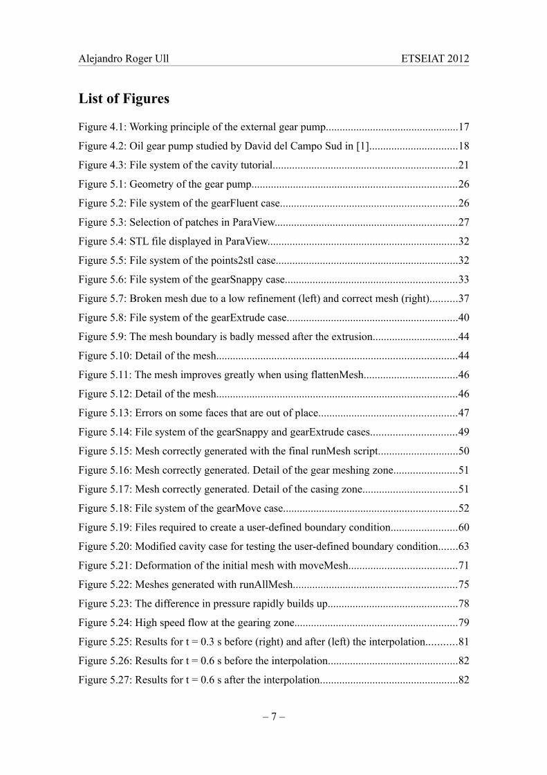
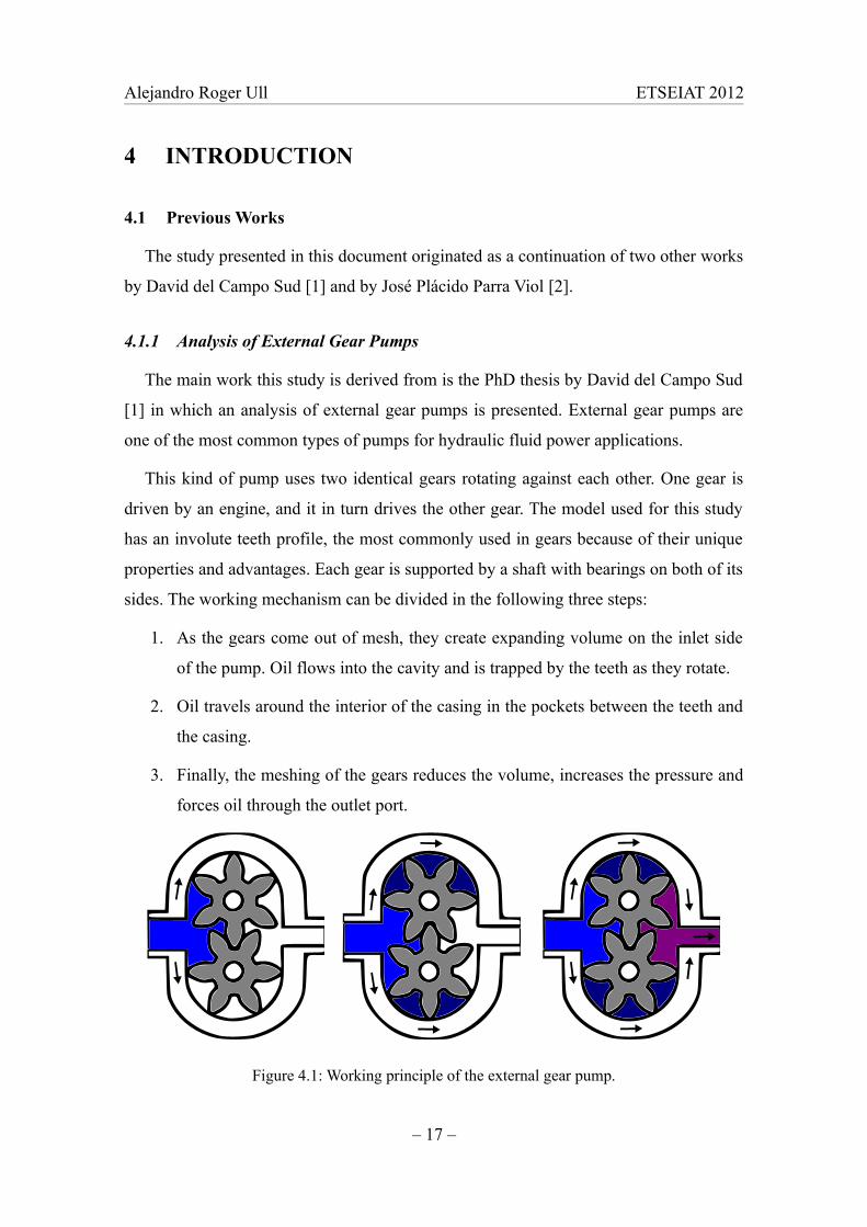
sides. The working mechanism can be divided in the following three steps:
1. As the gears come out of mesh, they create expanding volume on the inlet side
of the pump. Oil flows into the cavity and is trapped by the teeth as they rotate.
2. Oil travels around the interior of the casing in the pockets between the teeth and
the casing.
3. Finally, the meshing of the gears reduces the volume, increases the pressure and
forces oil through the outlet port.
Figure 4.1: Working principle of the external gear pump.
– 17 –
Alejandro Roger Ull ETSEIAT 2012
The main purpose of the thesis by David del Campo Sud is to analyze the effect
different forms of the suction chamber on cavitation, and the effect of cavitation on the
volumetric efficiency. To pursue this target both experimental and numerical analysis
were performed.
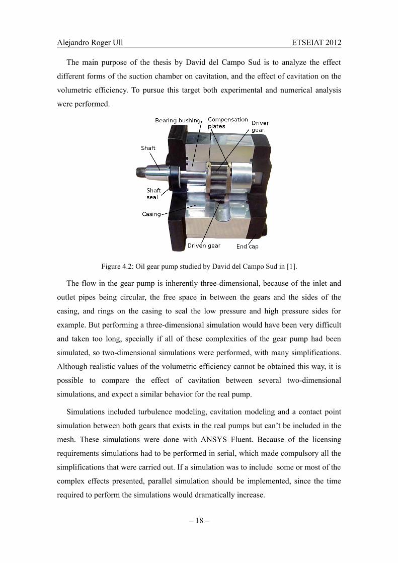
Figure 4.2: Oil gear pump studied by David del Campo Sud in [1].
The flow in the gear pump is inherently three-dimensional, because of the inlet and
outlet pipes being circular, the free space in between the gears and the sides of the
casing, and rings on the casing to seal the low pressure and high pressure sides for
example. But performing a three-dimensional simulation would have been very difficult
and taken too long, specially if all of these complexities of the gear pump had been
simulated, so two-dimensional simulations were performed, with many simplifications.
Although realistic values of the volumetric efficiency cannot be obtained this way, it is
possible to compare the effect of cavitation between several two-dimensional
simulations, and expect a similar behavior for the real pump.
Simulations included turbulence modeling, cavitation modeling and a contact point
simulation between both gears that exists in the real pumps but can’t be included in the
mesh. These simulations were done with ANSYS Fluent. Because of the licensing
requirements simulations had to be performed in serial, which made compulsory all the
simplifications that were carried out. If a simulation was to include some or most of the
complex effects presented, parallel simulation should be implemented, since the time
required to perform the simulations would dramatically increase.
– 18 –
Alejandro Roger Ull ETSEIAT 2012
It is because of this that the need to switch to open source software surged, with
which the ability to perform parallel simulations comes with no licensing costs.
4.1.2 Initial Study of Mesh Deformation with OpenFOAM
The first study for porting the work done by David del Campo Sud in [1] was started
by José Plácido Parra Viol in [2] in his final project. In short, in that study the dynamic
mesh solver is studied, a first implementation of the boundary conditions for rotating
objects is developed, and it is tested with a simple geometry, like the one depicted in
Figure 5.20 in this work.
Although the step forward done in that study was important, and some results of that
work are used here, the geometry used by José Plácido Parra Viol was so basic that it
could be easily meshed. It is because of this that most of the development presented in
the next section of this work is focused towards being able to run the simulation with an
arbitrary geometry, in this case the gear pump previously mentioned.
4.2 Dynamic Mesh
The handling of dynamic meshes is required in many simulations in which the
domain changes over time. This change can either be prescribed, such as with the gear
pump, where the gears rotate driven by an engine; or it can be dependent on the solution
of the flow, such as with aeroelasticiy simulations or any other kind of simulation where
a structure interacts with the fluid.
In the case of prescribed motion, like the one that is under study in this work, since
the movement is known beforehand, a sequence of meshes can be generated, so that
they are able to easily accommodate the motion of the boundaries. In between those
generated meshes the mesh can be deformed according to the prescribed boundary
movement. It is when the deformation of the mesh is excessive that the deformed mesh
can be replaced with a new generated one.
But the motion is prescribed at the boundaries, not at the entire mesh. The motion of
each point and cell in the mesh needs to be calculated so that the mesh adapts softly to
the domain changes. Automatic mesh motion must determine the position of those
points based on the prescribed motion of the boundary [6].
– 19 –
Alejandro Roger Ull ETSEIAT 2012
This is in fact a whole additional problem, that is added to the problem of solving the
flow. That is, boundary conditions for a property (the movement of the points) are
defined for a closed domain in which the solution for that property is to be found. Thus
the need for a mesh motion equation that has to be solved to find that solution for the
movement.
But this equation does not describe a real physical movement, it can be somehow
arbitrarily chosen so that it fits the purpose of the dynamic mesh handling adequately.
Initial studies trended to considerate the mesh like a solid, for which the deformation
was calculated with the finite volume method. Or also the so called spring analogy,
which considered the connection between each pair of points as a spring or a one-
dimensional bar with a known, prescribed stiffness.
But these methods didn’t worked as expected. For the finite volume method the
solution of the mesh motion was being obtained in the center of the cells, so the motion
of the points had to be interpolated, reducing the quality of the solution. As for the
spring analogy, although initially this method yields a linear set of equations, its bad
behavior forced the introduction of non-linearities that made the solution of the
movement of the mesh too computationally expensive to be used, sometimes even more
complex than that of the flow itself [2].
Nowadays, the use of a finite element method based on solving the Laplacian
equation for the velocity of the mesh points, ∇⋅(k ∇ u)=0 , either with a constant or
variable diffusivity k, is very extended. The added diffusivity acts as a control for the
mesh deformation and quality.
Additionally, it must be noted that the fluid equations that are going to be used to
solve the flow must be written for time-changing domains, instead of a stationary one,
for the conservation laws to be fulfilled.
Also, if mesh deformation is large or for some special uses, it could be interesting to
apply topological changes. These consist on changing the mesh with little or no
deformation, by making a part of the mesh move with respect to another one, for
instance, or by removing or adding a boundary, for example to simulate the opening and
closing of a valve inside a pipe. These methods are not under study in this work, but
they must be considered if these changes are adequate for the problem to be solved.
– 20 –
Alejandro Roger Ull ETSEIAT 2012
4.3 OpenFOAM Description
OpenFOAM (the name stands for Open Field Operation and Manipulation) is a free,
open source CFD software package. It has a large user base across most areas of
engineering and science, as OpenFOAM has an extensive range of features to solve
anything from complex fluid flows involving chemical reactions, turbulence and heat
transfer, to solid dynamics, electromagnetics and finances [4].
Its solvers range from incompressible and compressible flows, multiphase flows,
combustion, buoyancy-driven flows, heat transfer, particle methods and also solid
dynamics and electromagnetics, while providing an extended library functionality with
turbulence models, transport and rheology models, thermophysical models, lagrangian
particle tracking, and chemical reaction kinetics directly available from its source.
4.3.1 Usage
The pre-processing is done in OpenFOAM by editing the directories and text files
that conform a case, as it can be seen in the next section where this study is developed.
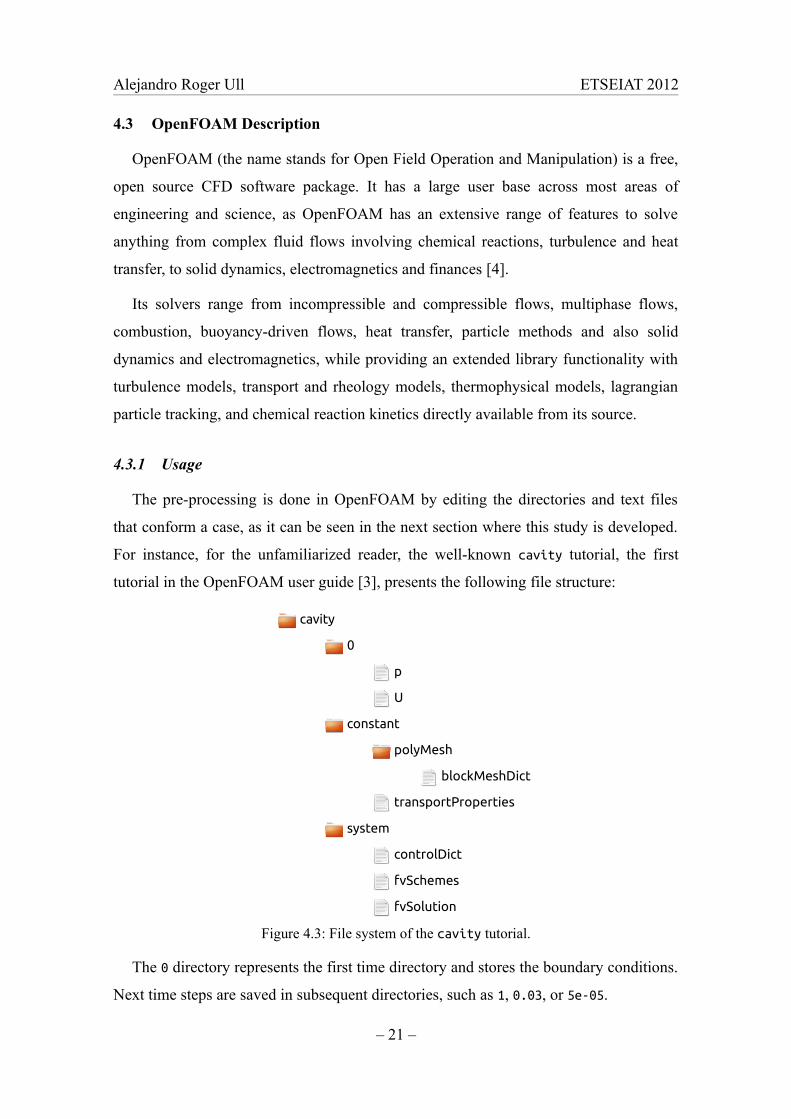
For instance, for the unfamiliarized reader, the well-known cavity tutorial, the first
tutorial in the OpenFOAM user guide [3], presents the following file structure:
cavity
0
p
U
constant
polyMesh
blockMeshDict
transportProperties
system
controlDict
fvSchemes
fvSolution
Figure 4.3: File system of the cavity tutorial.
The 0 directory represents the first time directory and stores the boundary conditions.
Next time steps are saved in subsequent directories, such as 1, 0.03, or 5e-05.
– 21 –
Alejandro Roger Ull ETSEIAT 2012
Inside the constant directory the properties of the problem that is going to be solved
are included, such as the mesh, the properties of the fluid, and other things if required.
The system directory contains all the controls of the simulation. Time steps, write
precision, etc. are determined in the controlDict file, whereas inside the fvSchemes file
the finite volume discretization schemes are determined for each time derivative,
gradient, divergence, laplacian, etc. In the fvSolution file the user can select the solver
that will calculate each variable. More dictionary files are required if certain
OpenFOAM tools are used.
Solvers and other OpenFOAM tools are run directly from the command-line
interface, also known as CLI or terminal. Post-processing can be done with the help of
an included program called ParaView.
OpenFOAM also counts with some tools to create meshes, from the basic blockMesh
to the more complex snappyHexMesh, and includes many tools for importing meshes
created with other software packages. Since it is heavily used in this document, should
the reader need it, the snappyHexMesh guide in section 5.4 of [3] can be consulted in case
of doubt.
4.3.2 Coding
But with no doubt the most important feature of OpenFOAM is the fact that it is
open-sourced. While OpenFOAM can be used as a standard simulation package, it
offers much more because it is designed to be a flexible, programmable environment for
simulation. Equations can be coded in a way much similar to that of its mathematical
notation. Take for instance the equation:
∂ρU∂ t
+∇⋅ρU U−∇⋅μ∇ U=−∇ p
In an OpenFOAM solver it can be represented by the code:
solve( fvm::ddt(rho, U) + fvm::div(phi, U) - fvm::laplacian(mu, U) == - fvc::grad(p));
– 22 –
Alejandro Roger Ull ETSEIAT 2012
It is because of this that OpenFOAM counts with some advantages with respect to
proprietary software, among which the following can be specially remarked:
• Users have total freedom to create their own solvers and libraries, which is
typically done by modifying an existing one.
• The solution algorithms are fully transparent, they can be viewed and checked
by the user, encouraging better understanding of the physics and equations
involved in the problem.
4.3.3 Parallel Execution
Also, OpenFOAM makes running cases in parallel easy. This permits solving more
complex problems in less time. Almost everything in OpenFOAM can be run in parallel,
and since OpenFOAM is free, compared to the per-processor licenses of commercial
software, parallel simulations are much more affordable.
In order to solve a case in parallel the domain is decomposed and each part is
allocated to a separate processor. OpenFOAM ships with the OpenMPI library to
manage the communications between processors and run parallel applications.
OpenFOAM is reported to scale well up to at least 1000 CPUs [4].
For further reference about how OpenFOAM works, the OpenFOAM User Guide [3]
and the OpenFOAM Features Guide [4] can be consulted.
4.3.4 Dynamic Mesh Implementation
The most logical implementation of the dynamic mesh in OpenFOAM in order to
solve the flow in the gear pump is that suggested by José Plácido Parra Viol in [2]. In
short description, the strategy is to generate multiple meshes for multiple positions of
the gears during one gearing cycle, so that once the mesh has deformed excessively
because of the rotation of the gears, a new mesh can be used.
Then the solver has to be run for multiple gearing cycles to ensure a certain level of
convergence, during which the same meshes can be reused multiple times, once per
cycle simulated. This implementation is developed in the next section.
– 23 –

Alejandro Roger Ull ETSEIAT 2012
5 DEVELOPMENT
5.1 Initial Case Setup
The study presented in this document is focused towards a particular problem,
although the developed procedure and its conclusions are of interest for any similar
dynamic mesh problem that is going to be solved in OpenFOAM.
In order to start the study, a work directory must be created. In OpenFOAM this is
typically accomplished by copying the files of an existing case to a new folder. The
existing case must be similar to the one in consideration, this way only a few files need
changes to work properly.
A good choice is to look among the tutorials provided with OpenFOAM for a case
with similar conditions. Tutorials are sorted by field (incompressible, compressible,
electromagnetics, financial, heat transfer, etc.), then by solver. Choosing the solver is an
important step in the early beginnings of the work, although it can be changed later. For
the gear pump simulation an incompressible solver capable of handling a dynamic mesh
is required. The choice is pimpleDyMFoam, a modified pimpleFoam that handles dynamic
meshes. It can do both laminar or turbulent simulations of transient incompressible flow.
The OpenFOAM tutorials are located in the following directory:
/opt/openfoamXYZ/tutorials/incompressible/pimpleDyMFoam
Where XYZ represents the OpenFOAM version. The version of OpenFOAM used in
this work is 2.1.0. Inside this directory one finds several tutorials. Two of them,
movingCone and wingMotion. are of interest. The former simulates the known, imposed
movement of an object across one axis, a movement similar to the one that is under
study. The latter simulates the movement of a two-dimensional airfoil caused by the
aerodynamic forces, its mesh being created with snappyHexMesh. A similar process will
be implemented to mesh the complex geometry this study faces.
Since both tutorials are of interest but none fulfill the scope of the study, the best
option is to manually create the new directories, copying the file system and the files
from one tutorial or the other as needed. Thus, a directory is created on the desktop,
called gearMain, inside of which all the other files will be placed.
– 25 –
Alejandro Roger Ull ETSEIAT 2012
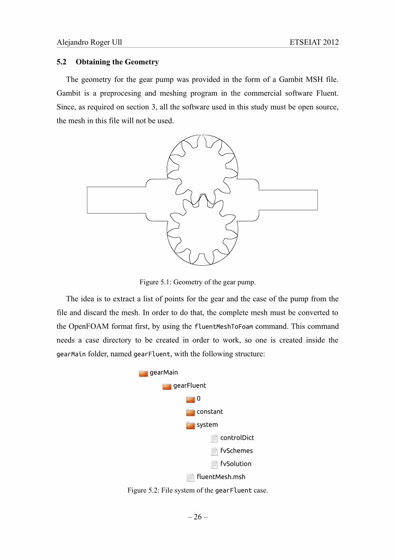
5.2 Obtaining the Geometry
The geometry for the gear pump was provided in the form of a Gambit MSH file.
Gambit is a preprocesing and meshing program in the commercial software Fluent.
Since, as required on section 3, all the software used in this study must be open source,
the mesh in this file will not be used.
Figure 5.1: Geometry of the gear pump.
The idea is to extract a list of points for the gear and the case of the pump from the
file and discard the mesh. In order to do that, the complete mesh must be converted to
the OpenFOAM format first, by using the fluentMeshToFoam command. This command
needs a case directory to be created in order to work, so one is created inside the
gearMain folder, named gearFluent, with the following structure:
gearMain
gearFluent
0
constant
system
controlDict
fvSchemes
fvSolution
fluentMesh.msh
Figure 5.2: File system of the gearFluent case.
– 26 –
Alejandro Roger Ull ETSEIAT 2012
The controlDict , fvSchemes and fvSolution files can be copied directly from the
wingMotion/wingMotion_snappyHexMesh tutorial. The user can adjust the write options
from the controlDict file (writeFormat, writePrecission and writeCompression) as
needed, but the default ones should be enough.
Once this case folder is all set the mesh can be converted by opening a terminal,
setting gearFluent as the working directory and entering the following command:
fluentMeshToFoam fluentMesh.msh
The mesh will be written inside the /constant/polyMesh directory. Once the mesh
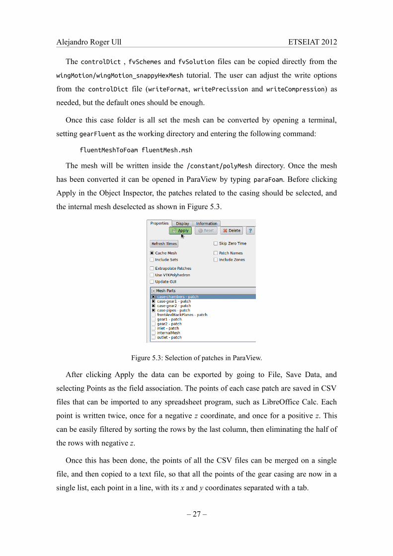
has been converted it can be opened in ParaView by typing paraFoam. Before clicking
Apply in the Object Inspector, the patches related to the casing should be selected, and
the internal mesh deselected as shown in Figure 5.3.
Figure 5.3: Selection of patches in ParaView.
After clicking Apply the data can be exported by going to File, Save Data, and
selecting Points as the field association. The points of each case patch are saved in CSV
files that can be imported to any spreadsheet program, such as LibreOffice Calc. Each
point is written twice, once for a negative z coordinate, and once for a positive z. This
can be easily filtered by sorting the rows by the last column, then eliminating the half of
the rows with negative z.
Once this has been done, the points of all the CSV files can be merged on a single
file, and then copied to a text file, so that all the points of the gear casing are now in a
single list, each point in a line, with its x and y coordinates separated with a tab.
– 27 –
Alejandro Roger Ull ETSEIAT 2012
This process must be repeated for one of the gears. In this case it is convenient to
rotate the points slightly so that a tooth of the gear is pointing directly upwards. This
way a single list of points will be valid for both gears, since the number of teeth is odd,
and by translating one upwards with respect to the other both will mesh perfectly.
The lower gear is centered on the coordinates origin, so this one will be the reference
gear. Again the points are extracted and filtered just as with the casing. To obtain the
angle that the points must be rotated, the geometry is inspected in ParaView. One can
obtain the coordinates of the center point of the uppermost tooth, and then calculate the
angle that the point must be rotated to reach the x = 0 plane.
Once all this work is done, the list of points for the casing and for the gear centered
at x,y = 0,0 has been obtained.
5.3 Generating an STL File
Before being able to mesh the geometry an STL file must be generated. This is
because the geometry will be meshed by using snappyHexMesh, which takes an STL file
as the input. STL files are standardized files that can be handled by many software
packages. Inside an STL file multiple solids can be represented as a list of triangles that
conform their surfaces. STL files can be written in ASCII or binary format. The ASCII
format looks like this:
solid name0facet normal n1 n2 n3
outer loopvertex x1 y1 z1vertex x2 y2 z2vertex x3 y3 z3
endloopendfacetfacet normal ......
endsolid name0solid name1...
Such a file can be written easily by hand if the geometry is simple enough, or with
the help of a small program if it is more complex. Many CAD softwares can export to
this file type too. In this case the most useful option is to write a program to read the
point list for the casing and the gear, then apply any desired transformation to the
geometry, such as a rotation to the gears, and finally write the geometry as an STL file.
– 28 –
Alejandro Roger Ull ETSEIAT 2012
This way it will be easy to automatically generate the geometry for any position of the
gears. Therefore, a short program, named points2stl.cpp, is written in C++ and then
compiled using the GNU Compiler Collection. To compile the program just enter into
the terminal:
g++ points2stl.cpp -o points2stl
And to run it:
./points2stl
The program requires several files to be present in its directory. A solids file must be
provided, for example as follows:
3 -1 11 gear0 1913 0 0 0 gear1 1913 0 45.123 0 case 1870 0 0 0
The first line indicates the number of solids below, then the minimum z value, and
the maximum z value for the STL file. Next, a line for each solid indicates the name, the
number of points, the translation in the x direction, the translation in the y direction, and
the rotation angle, in rad. Note how the gear1 solid is displaced towards the y direction.
This is because the same list of points is being used for both gears.
For each solid, another file with the name of the solid (in the example: gear0, gear1
and case) must be present in the same directory. This file must contain the points of the
solid as they were extracted in the previous section:
-2.6841909571 23.5344354143 -2.7402671858 23.4064052141 1.9790048057 24.8983171305 2.0492641836 24.7775481...
The points that were extracted in the previous section were not sorted consecutively.
Thus, the C++ program has to sort them during runtime. To do that, the program starts
with the first point and, to get the next one, it searches for the nearest point that hasn’t
been already selected. The program keeps going by taking one pair of points at a time.
Each of these pair of points is placed at the maxZ plane and a copy is placed at the minZ
plane. Finally the rectangle formed by these four vertices is split into two triangles and
written to the output STL file. For the last point, an exception is made so that it connects
with the first point and the STL surface is closed.
– 29 –
Alejandro Roger Ull ETSEIAT 2012
The C++ source code of the points2stl program is shown below, but it is also
included in the media that comes with this work.
1234567891011121314151617181920212223242526272829303132333435363738394041424344454647484950515253545556
#include<fstream>#include<cmath>
using namespace std;
bool isPastPoint(int point, int pastPoint[], int n){ int i; for (i=0;i<n;i++) if (point == pastPoint[i]) return 1; return 0;}
int getNextPoint(int curPoint, int pastPoint[], int n, int nPoints, double point[][2]){ int i, nextPoint; double x1, y1, x2, y2, distance2, minDistance2; //Special case for the last point to meet the first point: if (n==nPoints) return pastPoint[0]; x1 = point[curPoint][1]; y1 = point[curPoint][2]; nextPoint = -1; minDistance2 = 1.e10; for (i=0; i<nPoints; i++) { x2 = point[i][1]; y2 = point[i][2]; distance2 = (x2-x1)*(x2-x1)+(y2-y1)*(y2-y1); if (distance2 < minDistance2 and not isPastPoint(i,pastPoint,n)) { minDistance2 = distance2; nextPoint = i; } } return nextPoint;}
int main(){ int nSolids, nPoints, i, s; int curPoint, nextPoint; double x, y, r, angle, dx, dy, dAngle, z0, z1; char solidName[20]; ifstream solidsFile; ofstream outputFile; solidsFile.open("./solids"); outputFile.open("./triSurface.stl", ios::out | ios::trunc);
solidsFile>>nSolids>>z0>>z1;
– 30 –

Alejandro Roger Ull ETSEIAT 2012
57585960616263646566676869707172737475767778798081828384858687888990919293949596979899100101102103104105106107108109110111112113114115116
for (s=0; s<nSolids; s++) { solidsFile>>solidName>>nPoints>>dx>>dy>>dAngle; ifstream pointsFile; pointsFile.open(solidName); int pastPoint[nPoints]; double point[nPoints][2]; for (i=0; i<nPoints; i++) {pointsFile>>point[i][1]>>point[i][2];} pointsFile.close(); for (i=0; i<nPoints; i++) { x = point[i][1]; y = point[i][2]; r = sqrt(x*x + y*y); angle = atan2(y,x) + dAngle; point[i][1] = r * cos(angle) + dx; point[i][2] = r * sin(angle) + dy; } outputFile<<"solid "<<solidName<<"\n"; curPoint = 0; nextPoint = 0; i = 0; while (i<nPoints) { curPoint = nextPoint; pastPoint[i] = curPoint; i++; nextPoint = getNextPoint(curPoint, pastPoint, i, nPoints, point); x = point[curPoint][1]; y = point[curPoint][2]; dx = point[nextPoint][1]; dy = point[nextPoint][2]; outputFile<<" facet normal "<<(y-dy)<<" "<<(dx-x)<<" 0.0\n"; outputFile<<" outer loop\n"; outputFile<<" vertex "<< x<<" "<< y<<" "<<z0<<"\n"; outputFile<<" vertex "<<dx<<" "<<dy<<" "<<z0<<"\n"; outputFile<<" vertex "<<dx<<" "<<dy<<" "<<z1<<"\n"; outputFile<<" endloop\n endfacet\n"; outputFile<<" facet normal "<<(y-dy)<<" "<<(dx-x)<<" 0.0\n"; outputFile<<" outer loop\n"; outputFile<<" vertex "<< x<<" "<< y<<" "<<z0<<"\n"; outputFile<<" vertex "<< x<<" "<< y<<" "<<z1<<"\n"; outputFile<<" vertex "<<dx<<" "<<dy<<" "<<z1<<"\n"; outputFile<<" endloop\n endfacet\n"; } outputFile<<"endsolid "<<solidName<<"\n"; } solidsFile.close(); outputFile.close(); return 0;}
– 31 –
Alejandro Roger Ull ETSEIAT 2012
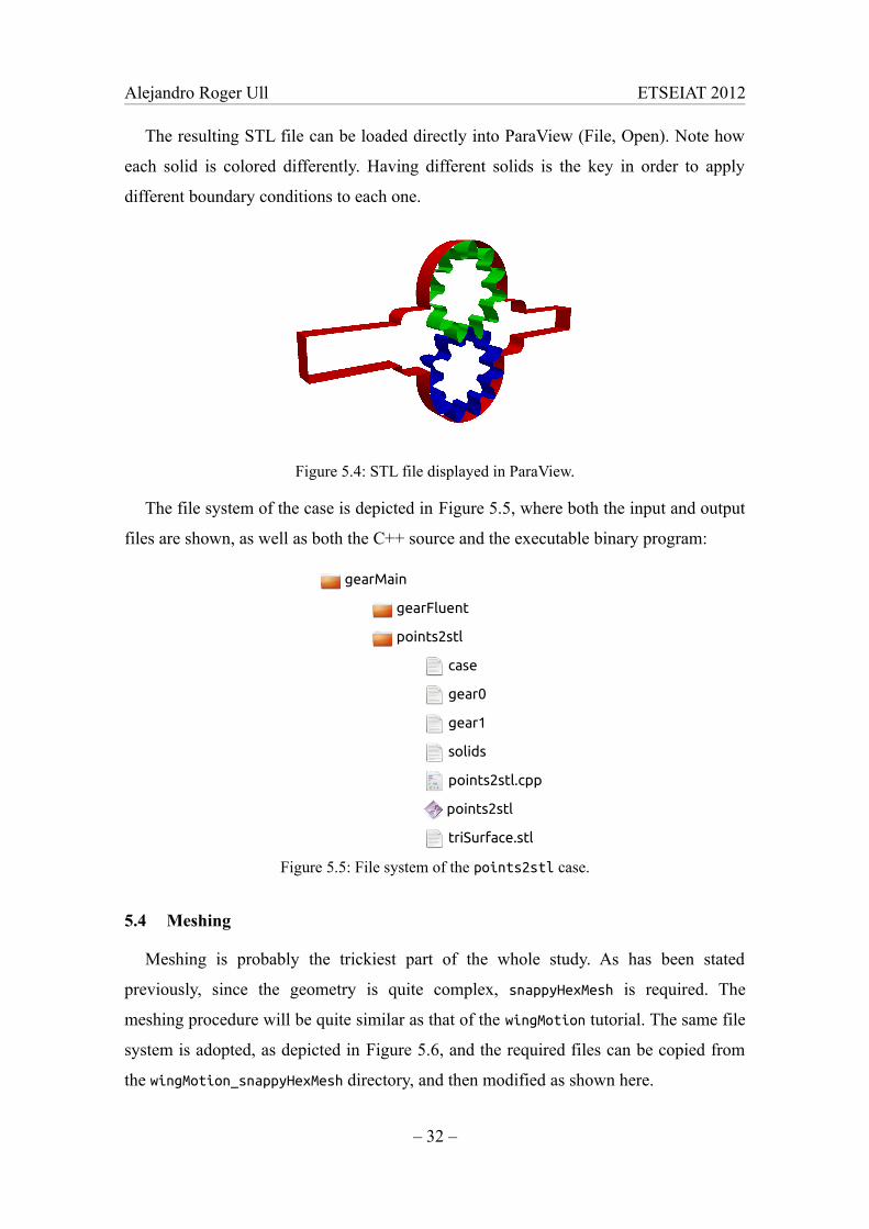
The resulting STL file can be loaded directly into ParaView (File, Open). Note how
each solid is colored differently. Having different solids is the key in order to apply
different boundary conditions to each one.
Figure 5.4: STL file displayed in ParaView.
The file system of the case is depicted in Figure 5.5, where both the input and output
files are shown, as well as both the C++ source and the executable binary program:
gearMain
gearFluent
points2stl
case
gear0
gear1
solids
points2stl.cpp
points2stl
triSurface.stl
Figure 5.5: File system of the points2stl case.
5.4 Meshing
Meshing is probably the trickiest part of the whole study. As has been stated
previously, since the geometry is quite complex, snappyHexMesh is required. The
meshing procedure will be quite similar as that of the wingMotion tutorial. The same file
system is adopted, as depicted in Figure 5.6, and the required files can be copied from
the wingMotion_snappyHexMesh directory, and then modified as shown here.
– 32 –
Alejandro Roger Ull ETSEIAT 2012
gearMain
gearFluent
points2stl
gearSnappy
0
constant
polyMesh
blockMeshDict
triSurface
triSurface.stl
system
controlDict fvSchemes
decomposeParDict fvSolution
snappyHexMeshDict
Figure 5.6: File system of the gearSnappy case.
5.4.1 blockMesh
Meshing with snappyHexMesh requires several actions to be performed. The first one
is to create a background mesh using blockMesh. The background mesh must be one-cell
thick in order to perform a two-dimensional simulation, with empty patches at its front
and back boundaries. The blockMeshDict file must be edited to create a mesh of the
approximate size of the STL geometry, which can be checked from ParaView.
The vertices and blocks description are as follows:
convertToMeters 1;
vertices (
//Front (-86 -30 0) //0 ( 86 -30 0) //1 ( 86 75 0) //2 (-86 75 0) //3 //Back (-86 -30 2) //4 ( 86 -30 2) //5 ( 86 75 2) //6 (-86 75 2) //7
);
– 33 –
Alejandro Roger Ull ETSEIAT 2012
blocks (
hex (0 1 2 3 4 5 6 7) (200 120 1) simpleGrading (1 1 1) );
Note that the dimensions of the block (and the STL file) are in millimeters. To work
in meters the whole mesh will have to be scaled at the end of the meshing process. This
is not strictly needed; OpenFOAM does not care about units, just dimensions. Thus it is
irrelevant if you work using the Imperial System, the Metric System, or any other
system (such as using millimeters for longitudes).
However one must take care, because all the input and output variables must share
the same units. So, to avoid any trouble this may cause, during the meshing process
longitudes will be in millimeters, but after that the Metric System will take over and the
mesh will be scaled to comply with it.
Next, no curved edges should appear in the block:
edges ( );
The rest of the blockMeshDict file defines the different boundaries:
boundary ( fixedWall { type wall; faces (
(0 1 5 4) //bottom (2 3 7 6) //top
); } inletPatch { type patch; faces ( (3 0 4 7) ); } outletPatch { type patch; faces ( (1 2 6 5) ); }
– 34 –

Alejandro Roger Ull ETSEIAT 2012
frontEmpty { type empty; faces (
(3 2 1 0) ); }
backEmpty { type empty; faces (
(4 5 6 7) ); } );
Finally, no pair of patches needs to be merged.
mergePatchPairs ( );
5.4.2 snappyHexMesh
Once the background mesh is created (by using the blockMesh command), it is time
for snappyHexMesh to refine the mesh and adapt it to the geometry that was just created
in STL format. The first entries of the snappyHexMeshDict file indicate the steps that will
be performed when snappyHexMesh runs. The layer addition process is not of interest for
this work, so let’s start with activating the castellated mesh and the snap processes first.
castellatedMesh true; snap true; addLayers false;
It will be seen further ahead that it is not a good idea to perform the snapping at this
point but let’s leave this as it is for now.
The next entry defines the file from which the geometry will be loaded, as well as
any refinement boxes the user may wish to define. The triSurface.stl file is loaded
from the ./constant/triSurface/ directory, and it is the file that was generated with
the points2stl C++ program.
At this point no refinement boxes will be used, but the entry is left in the file,
commented out, so that adding one box can be done quickly should the user want to.
– 35 –
Alejandro Roger Ull ETSEIAT 2012
geometry { triSurface.stl { type triSurfaceMesh; name gear; }
//refinementBox //{ // type searchableBox; // min (-30. -30. 0.); // max ( 30. 75. 10.); //} };
Next in the file are the controls for the castellatedMesh. The first controls set limits
to the process in terms of number of cells. The values can be adjusted at user discretion,
the ones presented here worked reasonably well:
castellatedMeshControls { maxLocalCells 700000; maxGlobalCells 1400000; minRefinementCells 10; maxLoadUnbalance 0.10; nCellsBetweenLevels 3;
Next, the explicit feature edge refinement is a feature (forgive the repetition) recently
added to OpenFOAM, that allows a better discretization on certain edges the domain
may have, which previously experienced some distortion. Since the mesh under study is
two-dimensional no edge should have this problem, and this feature is commented out:
features ( //{ // file "someLine.eMesh"; // level 2; //} );
After a score of tests the levels of refinement presented here were selected as the best
choice in terms of quality and time. Too much refinement implies a much higher
meshing time, which would be prohibitive if one recalls that multiple meshes are going
to be made.
On the other hand, too low levels would split the mesh at points where the teeth and
the case are so close that the mesh after those points would be marked as unreachable
and removed from the rest of the mesh, as seen on Figure 5.7.
– 36 –

Alejandro Roger Ull ETSEIAT 2012
Figure 5.7: Broken mesh due to a low refinement (left) and correct mesh (right).
Again the refinement regions entry is commented out, since no refinement boxes are
being used. If refinement boxes are being used, the user must uncomment these too.
refinementSurfaces { gear { level (3 5); } } resolveFeatureAngle 30;
refinementRegions { //refinementBox //{ // mode inside; // levels ((1E15 2)); //} }
Finally the last castellatedMesh controls are listed. The locationInMesh is selected
so that it is not in a face of any cell, but inside a cell. Any part of the mesh that cannot
be reached from this point after refinement is eliminated. As it has been said, if the
refinement is not high enough, the part of the mesh behind the teeth will be deleted.
locationInMesh (-85.91 15.01 0.0000000005); allowFreeStandingZoneFaces true; }
Next the snapping controls are left more or less at the default values:
snapControls { nSmoothPatch 3; tolerance 4.0; nSolveIter 3; nRelaxIter 5; //nFeatureSnapIter 10; }
– 37 –
Alejandro Roger Ull ETSEIAT 2012
Since the layer addition process was deactivated at the beginning of the file, those
controls are of no interest. The mesh quality controls are left at default values too, so the
snappyHexMeshDict file is ready.
However, several problems arise when trying to perform the snappyHexMesh run.
First, all programs in OpenFOAM are three-dimensional, and snappyHexMesh is not an
exception. Because of this, snappyHexMesh refines the mesh through the z direction,
obliterating the one-cell thickness that was selected with blockMesh.
This is a huge drawback, because to perform a two-dimensional simulation in
OpenFOAM the mesh must have this one-cell thickness and empty front and back
patches. By adding cells through the z direction, snappyHexMesh renders the mesh
useless. Also, the process of snapping takes much longer than expected, which is a
problem if multiple meshes are to be generated at different positions of the gears.
The following steps are needed to solve these problems. First, parallel execution of
snappyHexMesh is developed in order to cut down meshing times. Next the mesh is made
two-dimensional again with help of the extrudeMesh tool.
5.4.3 decomposePar
The parallel processing is performed by splitting the domain into multiple sub-cases
folders, then the solver (or the meshing program in this case) runs all cases at once,
keeping them in communication. In OpenFOAM this can be done automatically by
means of the decomposePar tool. As with most OpenFOAM applications, the
decomposePar tool requires its own decomposeParDict file.
Given that the computer in which the meshing is being executed has an eight-core
Intel i7 processing unit, six of those cores are utilized to perform the parallel meshing.
The decomposing method is hierarchical, a simple method that divides the domain in
equal parts in the number and order specified for each direction.
numberOfSubdomains 6; method hierarchical;
hierarchicalCoeffs { n (3 2 1); delta 0.001; order xyz; }
– 38 –
Alejandro Roger Ull ETSEIAT 2012
The domain can now be decomposed by running the decomposePar command after
running the blockMesh command. Six folders are created, named processor0 to
processor5, inside the gearSnappy directory. Inside each of those folders a sixth of the
background mesh is set for refinement. It is recommended to run the following
command just after decomposing the domain, before the snappyHexMesh process:
foamJob -s -p renumberMesh -overwrite
Then the snapping is run by entering the command:
foamJob -s -p snappyHexMesh -overwrite
The foamJob command allows the execution of OpenFOAM applications with some
special options, and parallel processing is one of them. This command stores all
command-line output to a log file. The -s option forces this output to be displayed in the
Terminal too. The -p option executes the application in parallel. The -overwrite option
forces renumberMesh and snappyHexMesh to overwrite the background mesh with the
renumbered or refined mesh, instead of storing it in a new time directory.
The renumberMesh tool reorders the numbering of the points in each processor
directory in order to make it more efficient.
During the snappyHexMesh process the load of each processor is balanced after each
step, if needed, in order to even the load of all of them up to a certain margin specified
in the maxLoadUnbalance entry in the snappyHexMeshDict file.
Once the meshing process is over the mesh can be reconstructed by using the
following command:
reconstructParMesh -mergeTol 1e-6 -constant
The -mergeTol option can be adjusted as needed, while the -constant option
indicates to the reconstructParMesh tool that the mesh is stored in the
./constant/polyMesh directory, and works in conjunction with the -overwrite option of
snappyHexMesh. In case the -overwrite option was not used, the option -time N (where
N is the time directory in which the mesh was stored), or the option -latestTime if the
mesh is stored in the last directory, can be used.
After the mesh has been reconstructed the processor0 to processor5 folders can be
deleted and the mesh is ready for the next step.
– 39 –

Alejandro Roger Ull ETSEIAT 2012
5.4.4 extrudeMesh
As it has been said, snappyHexMesh refines the mesh in all directions, including the z
direction. This makes the mesh unusable as a two-dimensional mesh. But there is a tool
called extrudeMesh that can generate a mesh by extruding a patch of another mesh. It is
used in the wingMotion tutorial, and as it can be seen, it requires a separate case
directory in order to work.
gearMain
gearFluent
points2stl
gearSnappy
gearExtrude
0
constant
system
controlDict fvSchemes
createPatchDict fvSolution
extrudeMeshDict
Figure 5.8: File system of the gearExtrude case.
The extrudeMeshDict file contains all the information needed in order to perform the
extrusion.
constructFrom patch; sourceCase "../gearSnappy"; sourcePatches (frontEmpty); exposedPatchName backEmpty; flipNormals false; extrudeModel linearNormal; nLayers 1; expansionRatio 1.0;
linearNormalCoeffs { thickness 1.0; }
mergeFaces false;
The constructFrom entry indicates that a patch from a mesh is going to be used as
the base for the extrusion. The source case is set to the gearSnappy directory, which is
located in the same directory as gearExtrude. The frontEmpty patch is selected as the
– 40 –
Alejandro Roger Ull ETSEIAT 2012
source patch, and the patch that is going to be created in front of it is called backEmpty.
The extrusion is chosen to be linear, as the target is to obtain a two-dimensional mesh.
This tool can generate also spherical or cylindrical extrusions. The number of cells the
mesh must have is one, as indicated by the nLayers entry. The expansionRatio and the
thickness have no special influence on the two-dimensional mesh, and the mergeFaces
entry is interesting only for 360° cylindrical extrusions.
As a side note, it is interesting to know that the extrudeMesh tool can also extrude a
two-dimensional surface mesh stored in a surface file such as an STL. In such a case the
first lines of the extrudeMeshDict file should read like this:
constructFrom surface; surface "./constant/triSurface/mesh.stl"; flipNormals false;...
This is interesting because the user may like to create the two-dimensional mesh
using another meshing software, such as Salome, instead of using snappyHexMesh, and
then the mesh could be exported as an STL file from that software and easily imported
into OpenFOAM using extrudeMesh.
In this case it should be noted that the definition of the vertices of all triangles in the
STL file must follow the right-hand rule to determine the normal to the surface and the
direction of the extrusion.
Back to the topic, a createPatchDict file is also added, its main interest being
renaming the patches created by the extrudeMesh tool, and, most important, removing
the fixedWall patches that were defined on top and bottom of the background
blockMesh, and that are not used after the snappyHexMesh process takes place.
pointSync false;
patches ( { name gear0; patchInfo { type wall; }
constructFrom patches; patches (gear_gear0); }
– 41 –
Alejandro Roger Ull ETSEIAT 2012
{ name gear1;
patchInfo { type wall; }
constructFrom patches; patches (gear_gear1); }
{ name case;
patchInfo { type wall; }
constructFrom patches; patches (gear_case); } );
The names of the patches could be different from those created by snappyHexMesh,
but there is no need to do so anyway. Only the gear_ part of the name is removed from
those patches. So the only important effect of running createPatch is removing the
unused patches, fixedWall in this case, from the mesh.
5.4.5 runMesh
After all the steps to generate a mesh from the STL file created in section 5.3 have
been defined, a small bash script called runMesh is written in order to automate the
execution of all the applications. It is placed inside the gearMain directory. Initially it
looks like this:
#!/bin/bash
. /opt/openfoam210/etc/bashrc
#snappyHexMeshcd gearSnappyrm -rf log processor* constant/polyMesh/*cp constant/blockMeshDictCopy constant/polyMesh/blockMeshDict
blockMeshdecomposeParfoamJob -s -p renumberMesh -overwrite foamJob -s -p snappyHexMesh -overwrite reconstructParMesh -mergeTol 1e-6 -constant
– 42 –

Alejandro Roger Ull ETSEIAT 2012
rm -rf processor*
#extrudeMeshcd ../gearExtruderm -rf constant/polyMesh/*extrudeMeshcreatePatch -overwrite
#scale to mmtransformPoints -scale "(0.001 0.001 0.001)"
Bash is just a scripting language that can automate the commands that are going to be
introduced in the Terminal. Each line in the bash script is a command that is entered into
the Terminal as if the user did so manually, and once that command ends the next one is
entered.
Several commands have been added to complete the procedure. The first command,
. /opt/openfoam210/etc/bashrc, is the same that must be included in the user’s
~/.bashrc file during installation of OpenFOAM in order to be able to use OpenFOAM
commands. This ensures that when launching the bash script OpenFOAM commands
will be available.
Next, the working directory changes to gearSnappy, and the files inside the
constant/polyMesh directory are removed, as well as any processor* folder that could
have been left at a previous run. After this, a copy of the blockMeshDict file that is
saved as constant/blockMeshDictCopy is moved into the constant/polyMesh directory,
and then blockMesh is run. This is done to ensure that a clean mesh is being used as the
background mesh for snappyHexMesh.
After running blockMesh the mesh is decomposed, renumbered in parallel, and then
snappyHexMesh runs in parallel too. After the mesh is reconstructed the processor
folders are removed again.
Finally, the working directory is changed to extrudeMesh, where again the
constant/polyMesh directory is cleaned, and the extrudeMesh and createPatch
commands are run. As it was said in section 5.4.1 the mesh is scaled at the end of the
complete meshing process, as to be dimensioned according to the Metric System.
Once the runMesh script finishes running, a two-dimensional mesh is obtained inside
the gearExtrude/constant/polyMesh directory.
– 43 –
Alejandro Roger Ull ETSEIAT 2012
5.4.6 Improving the Meshing Procedure
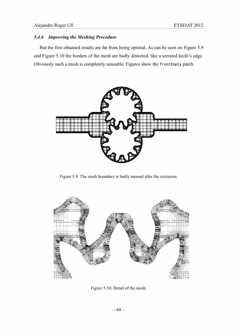
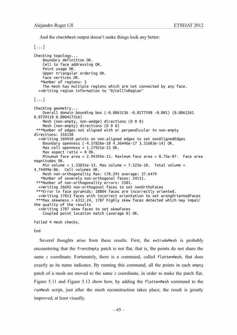
But the first obtained results are far from being optimal. As can be seen on Figure 5.9
and Figure 5.10 the borders of the mesh are badly distorted, like a serrated knife’s edge.
Obviously such a mesh is completely unusable. Figures show the frontEmpty patch.
Figure 5.9: The mesh boundary is badly messed after the extrusion.
Figure 5.10: Detail of the mesh.
– 44 –
Alejandro Roger Ull ETSEIAT 2012
And the checkMesh output doesn’t make things look any better:
[...]
Checking topology... Boundary definition OK. Cell to face addressing OK. Point usage OK. Upper triangular ordering OK. Face vertices OK. *Number of regions: 5 The mesh has multiple regions which are not connected by any face. <<Writing region information to "0/cellToRegion"
[...]
Checking geometry... Overall domain bounding box (-0.0863136 -0.0277598 -0.001) (0.0861261 0.0729118 0.000417316) Mesh (non-empty, non-wedge) directions (0 0 0) Mesh (non-empty) directions (0 0 0) ***Number of edges not aligned with or perpendicular to non-empty directions: 316150 <<Writing 169410 points on non-aligned edges to set nonAlignedEdges Boundary openness (-4.57826e-18 4.36446e-17 3.31683e-14) OK. Max cell openness = 1.27921e-15 OK. Max aspect ratio = 0 OK. Minumum face area = 2.94395e-11. Maximum face area = 8.75e-07. Face area magnitudes OK. Min volume = 1.33031e-13. Max volume = 7.525e-10. Total volume = 4.74499e-06. Cell volumes OK. Mesh non-orthogonality Max: 178.291 average: 37.6479 *Number of severely non-orthogonal faces: 24111. ***Number of non-orthogonality errors: 2581. <<Writing 26692 non-orthogonal faces to set nonOrthoFaces ***Error in face pyramids: 18804 faces are incorrectly oriented. <<Writing 17013 faces with incorrect orientation to set wrongOrientedFaces ***Max skewness = 6312.24, 1787 highly skew faces detected which may impair the quality of the results <<Writing 1787 skew faces to set skewFaces Coupled point location match (average 0) OK.
Failed 4 mesh checks.
End
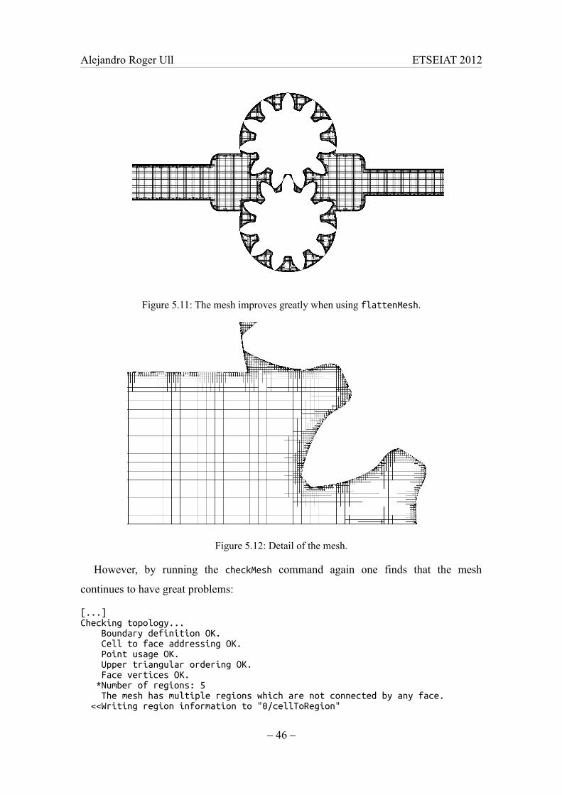
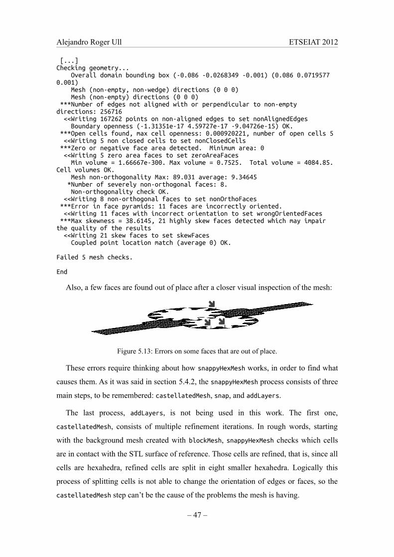
Several thoughts arise from these results. First, the extrudeMesh is probably
encountering that the frontEmpty patch is not flat, that is, the points do not share the
same z coordinate. Fortunately, there is a command, called flattenMesh, that does
exactly as its name indicates. By running this command, all the points in each empty
patch of a mesh are moved to the same z coordinate, in order to make the patch flat.
Figure 5.11 and Figure 5.12 show how, by adding the flattenMesh command to the
runMesh script, just after the mesh reconstruction takes place, the result is greatly
improved, at least visually.
– 45 –
Alejandro Roger Ull ETSEIAT 2012
Figure 5.11: The mesh improves greatly when using flattenMesh.
Figure 5.12: Detail of the mesh.
However, by running the checkMesh command again one finds that the mesh
continues to have great problems:
[...]Checking topology... Boundary definition OK. Cell to face addressing OK. Point usage OK. Upper triangular ordering OK. Face vertices OK. *Number of regions: 5 The mesh has multiple regions which are not connected by any face. <<Writing region information to "0/cellToRegion"
– 46 –
Alejandro Roger Ull ETSEIAT 2012
[...]Checking geometry... Overall domain bounding box (-0.086 -0.0268349 -0.001) (0.086 0.0719577 0.001) Mesh (non-empty, non-wedge) directions (0 0 0) Mesh (non-empty) directions (0 0 0) ***Number of edges not aligned with or perpendicular to non-empty directions: 256716 <<Writing 167262 points on non-aligned edges to set nonAlignedEdges Boundary openness (-1.31351e-17 4.59727e-17 -9.04726e-15) OK. ***Open cells found, max cell openness: 0.000920221, number of open cells 5 <<Writing 5 non closed cells to set nonClosedCells ***Zero or negative face area detected. Minimum area: 0 <<Writing 5 zero area faces to set zeroAreaFaces Min volume = 1.66667e-300. Max volume = 0.7525. Total volume = 4084.85. Cell volumes OK. Mesh non-orthogonality Max: 89.031 average: 9.34645 *Number of severely non-orthogonal faces: 8. Non-orthogonality check OK. <<Writing 8 non-orthogonal faces to set nonOrthoFaces ***Error in face pyramids: 11 faces are incorrectly oriented. <<Writing 11 faces with incorrect orientation to set wrongOrientedFaces ***Max skewness = 38.6145, 21 highly skew faces detected which may impair the quality of the results <<Writing 21 skew faces to set skewFaces Coupled point location match (average 0) OK.
Failed 5 mesh checks.
End
Also, a few faces are found out of place after a closer visual inspection of the mesh:
Figure 5.13: Errors on some faces that are out of place.
These errors require thinking about how snappyHexMesh works, in order to find what
causes them. As it was said in section 5.4.2, the snappyHexMesh process consists of three
main steps, to be remembered: castellatedMesh, snap, and addLayers.
The last process, addLayers, is not being used in this work. The first one,
castellatedMesh, consists of multiple refinement iterations. In rough words, starting
with the background mesh created with blockMesh, snappyHexMesh checks which cells
are in contact with the STL surface of reference. Those cells are refined, that is, since all
cells are hexahedra, refined cells are split in eight smaller hexahedra. Logically this
process of splitting cells is not able to change the orientation of edges or faces, so the
castellatedMesh step can’t be the cause of the problems the mesh is having.
– 47 –

Alejandro Roger Ull ETSEIAT 2012
Then the only left cause for these problems is the snap process. Supposedly, during
this step the points and faces are moved and aligned with the STL surface. But since, as
it has been said, OpenFOAM in general and snappyHexMesh in particular work with
three-dimensional domains, while the mesh that one wants to obtain in this case is two-
dimensional. And since after the castellatedMesh step the mesh has multiple cells in
the z direction, the snap process modifies the orientation of faces and cells in this
direction, and badly deteriorates the mesh for the later two-dimensional extrusion.
It is because of this that a new strategy is developed. Until now the wingMotion
tutorial has been closely followed, using first the castellateMesh and snap processes,
and then extruding the two-dimensional, desired mesh. But now this order will be
modified.
First, only the castellateMesh step of snappyHexMesh will be run, avoiding potential
misalignment problems. Next, the mesh will be flattened just in case; since no snap is
performed up to this point the flattenMesh step may be useless, but it is better to
prevent than to heal. After this the mesh can be extruded and finally snappyHexMesh is
run again, this time with snap only.
The file system is arranged as shown in Figure 5.14. This strategy implies having an
additional snappyHexMeshDict file, as well as a copy of the triSurface.stl file, inside
the gearExtrude directory. The decomposeParDict file is needed by snappyHexMesh,
although for the second time snappyHexMesh runs, after extrudeMesh, the domain will
not be decomposed, as after the mesh is made two-dimensional the snap process should
run quick enough.
The gearSnappy/system/snappyHexMeshDict file reads at the top lines:
castellatedMesh true;snap false;addLayers false;
While the one at gearExtrude/system/snappyHexMeshDict reads:
castellatedMesh false;snap true;addLayers false;
This way the snap won’t take place until the mesh has been extruded.
– 48 –

Alejandro Roger Ull ETSEIAT 2012
gearMain
gearFluent
points2stl
gearSnappy
0
constant
blockMeshDictCopy
polyMesh
blockMeshDict
triSurface
triSurface.stl
system
controlDict fvSchemes
decomposeParDict fvSolution
snappyHexMeshDict
gearExtrude
0
constant
triSurface
triSurface.stl
system
controlDict decomposeParDict
createPatchDict fvSchemes
extrudeMeshDict fvSolution
snappyHexMeshDict
runMesh
Figure 5.14: File system of the gearSnappy and gearExtrude cases.
Apart from these changes, the patches must now keep the same name between the
two snappyHexMesh runs. Therefore, the createPatch run is moved to after the second
snappyHexMesh run, in order to rename the gear patches and, most important, remove the
unused fixedWall patch.
The backup copy of the blockMeshDict file, blockMeshDictCopy is shown in Figure
5.14 too.
– 49 –
Alejandro Roger Ull ETSEIAT 2012
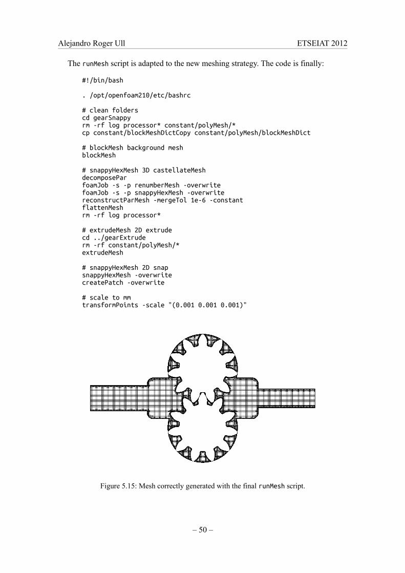
The runMesh script is adapted to the new meshing strategy. The code is finally:
#!/bin/bash
. /opt/openfoam210/etc/bashrc
# clean folderscd gearSnappy rm -rf log processor* constant/polyMesh/* cp constant/blockMeshDictCopy constant/polyMesh/blockMeshDict
# blockMesh background meshblockMesh
# snappyHexMesh 3D castellateMeshdecomposePar foamJob -s -p renumberMesh -overwrite foamJob -s -p snappyHexMesh -overwrite reconstructParMesh -mergeTol 1e-6 -constant flattenMesh rm -rf log processor*
# extrudeMesh 2D extrude cd ../gearExtrude rm -rf constant/polyMesh/*extrudeMesh
# snappyHexMesh 2D snap snappyHexMesh -overwrite createPatch -overwrite
# scale to mm transformPoints -scale "(0.001 0.001 0.001)"
Figure 5.15: Mesh correctly generated with the final runMesh script.
– 50 –
Alejandro Roger Ull ETSEIAT 2012
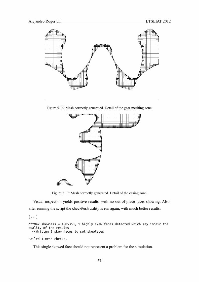
Figure 5.16: Mesh correctly generated. Detail of the gear meshing zone.
Figure 5.17: Mesh correctly generated. Detail of the casing zone.
Visual inspection yields positive results, with no out-of-place faces showing. Also,
after running the script the checkMesh utility is run again, with much better results:
[...]
***Max skewness = 4.05358, 1 highly skew faces detected which may impair the quality of the results <<Writing 1 skew faces to set skewFaces
Failed 1 mesh checks.
This single skewed face should not represent a problem for the simulation.
– 51 –
Alejandro Roger Ull ETSEIAT 2012
5.5 Moving the Mesh
Once a mesh has been generated it is time to start moving it. The target is to check
how much the gears can rotate, and how much deformation the mesh can withstand,
before the deformation becomes too much and a new mesh is needed to take over.
First of all a new case directory is created. Secondly the boundary conditions for
pressure and velocity, as well as the movement of the mesh, are introduced into the case.
Next a new boundary condition for the rotating motion of the gears is developed. After
that the different parameters of the case are determined. And finally a bash script is
written to run the moving of the mesh.
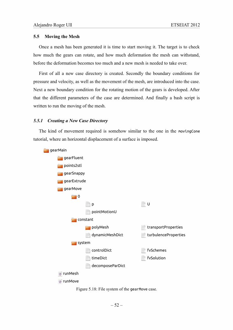
5.5.1 Creating a New Case Directory
The kind of movement required is somehow similar to the one in the movingCone
tutorial, where an horizontal displacement of a surface is imposed.
gearMain
gearFluent
points2stl
gearSnappy
gearExtrude
gearMove
0
p U
pointMotionU
constant
polyMesh transportProperties
dynamicMeshDict turbulenceProperties
system
controlDict fvSchemes
timeDict fvSolution
decomposeParDict
runMesh
runMove
Figure 5.18: File system of the gearMove case.
– 52 –
Alejandro Roger Ull ETSEIAT 2012
In the case of the gears the displacement is also imposed, but it being a rotation and
not a translation will enforce changes in most files concerning the dynamic mesh.
Nevertheless the movingCone tutorial is similar enough, and the file system of the
gearMove case is based on it, as shown in Figure 5.18.
5.5.2 Setting Up the Boundary Conditions
The boundary conditions of an OpenFOAM case are defined inside the first time
directory, 0 in this case. Inside the 0 directory there is a file for each field considered,
where boundary conditions are defined in a per-patch basis, that is, each patch may have
a different boundary condition. The same is true in reverse order: for two surfaces to
have different boundary conditions they must be defined as separate patches.
Boundary conditions for the pressure p and the velocity U are chosen among the ones
available in OpenFOAM. First, the pressure file p is shown here by sections. The header
reads:
FoamFile { version 2.0; format ascii; class volScalarField; object p; }
In the class entry it is indicated that the pressure is a volumetric scalar field. This
will have some importance regarding the boundary file for the motion of the gears.
dimensions [0 2 -2 0 0 0 0];
internalField uniform 0;
Dimensions are specified as powers of the fundamental dimensions. As it was
mentioned previously, OpenFOAM does not use any units inherently. Operations must
be performed using consistent units of measurement; in particular, addition, subtraction
and equality are only physically meaningful for properties of the same dimensional
units. As a safeguard against implementing a meaningless operation, OpenFOAM
attaches dimensions to field data and physical properties and performs dimension
checking on any tensor operation [3]. As long as dimensions agree the user can choose
any set of units. Table 5.1 shows the order in which dimensions are defined, as well as
typical working units.
– 53 –
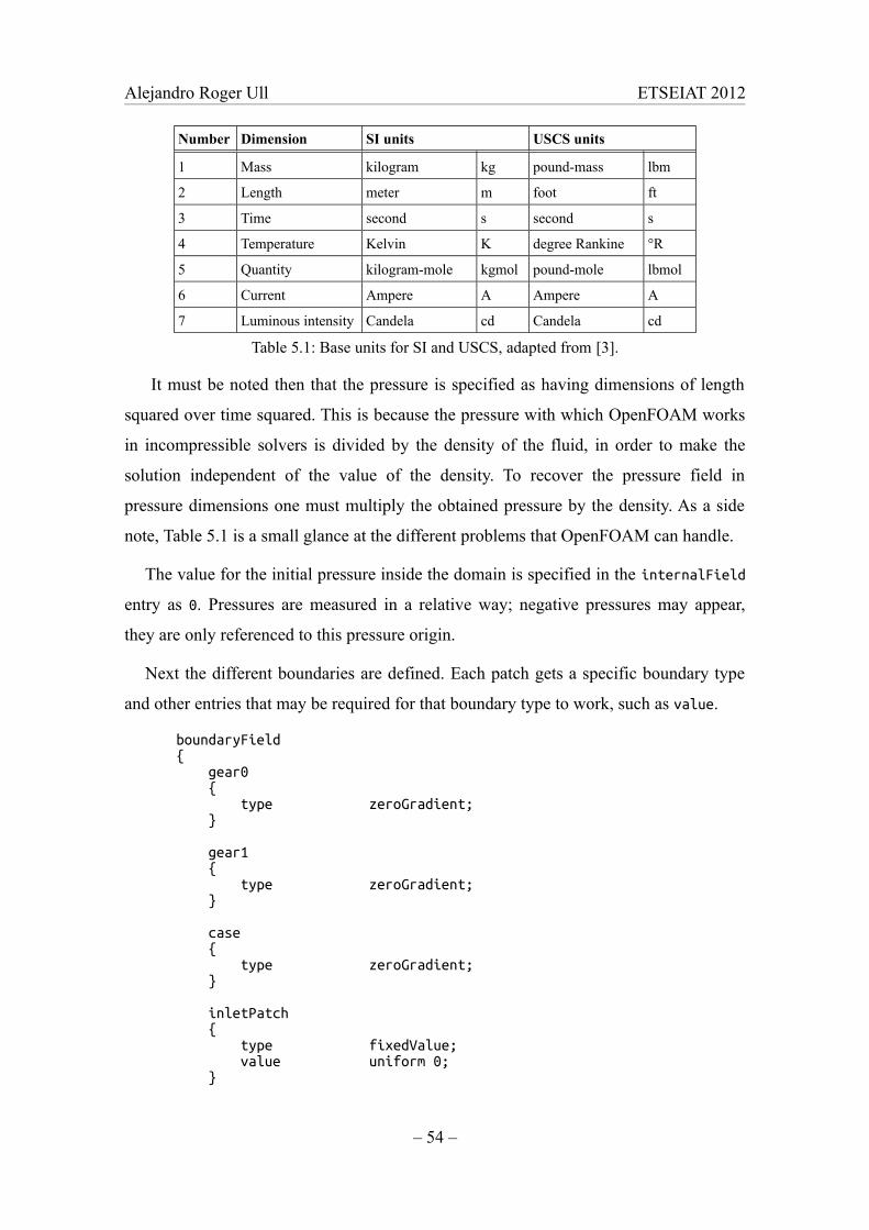
Alejandro Roger Ull ETSEIAT 2012
Number Dimension SI units USCS units
1 Mass kilogram kg pound-mass lbm
2 Length meter m foot ft
3 Time second s second s
4 Temperature Kelvin K degree Rankine °R
5 Quantity kilogram-mole kgmol pound-mole lbmol
6 Current Ampere A Ampere A
7 Luminous intensity Candela cd Candela cd
Table 5.1: Base units for SI and USCS, adapted from [3].
It must be noted then that the pressure is specified as having dimensions of length
squared over time squared. This is because the pressure with which OpenFOAM works
in incompressible solvers is divided by the density of the fluid, in order to make the
solution independent of the value of the density. To recover the pressure field in
pressure dimensions one must multiply the obtained pressure by the density. As a side
note, Table 5.1 is a small glance at the different problems that OpenFOAM can handle.
The value for the initial pressure inside the domain is specified in the internalField
entry as 0. Pressures are measured in a relative way; negative pressures may appear,
they are only referenced to this pressure origin.
Next the different boundaries are defined. Each patch gets a specific boundary type
and other entries that may be required for that boundary type to work, such as value.
boundaryField { gear0 { type zeroGradient; }
gear1 { type zeroGradient; }
case { type zeroGradient; }
inletPatch { type fixedValue; value uniform 0; }
– 54 –
Alejandro Roger Ull ETSEIAT 2012
outletPatch { type zeroGradient; }
frontEmpty { type empty; }
backEmpty { type empty; } }
It can be seen how pressure is fixed to a specific reference value at the inlet, and set
to having no gradient in the direction normal to the boundary for the rest of the patches.
The frontEmpty and backEmpty patches are special in the way that they are defined as
empty for the simulation to be two-dimensional.
Similarly, for the velocity boundary conditions the header of the U file reads:
FoamFile { version 2.0; format ascii; class volVectorField; object U; }
Here the velocity field is defined as being a vector field, naturally. Dimensions are
specified as expected.
dimensions [0 1 -1 0 0 0 0];
internalField uniform (0 0 0);
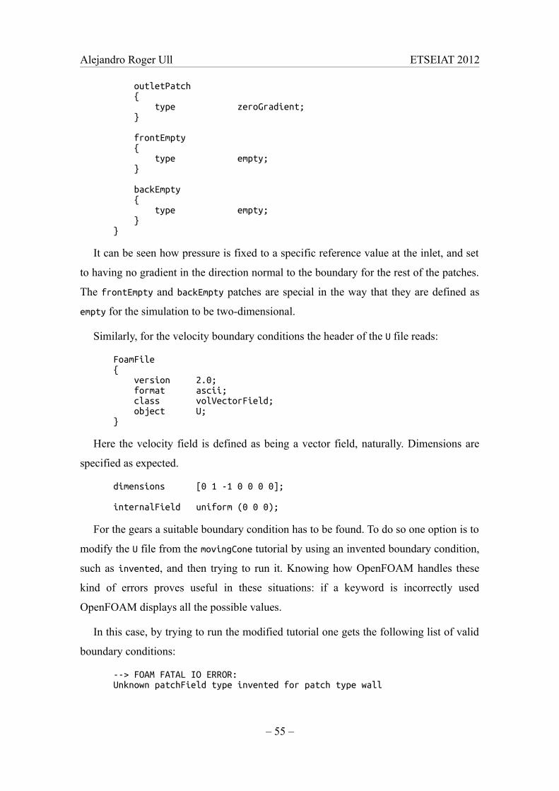
For the gears a suitable boundary condition has to be found. To do so one option is to
modify the U file from the movingCone tutorial by using an invented boundary condition,
such as invented, and then trying to run it. Knowing how OpenFOAM handles these
kind of errors proves useful in these situations: if a keyword is incorrectly used
OpenFOAM displays all the possible values.
In this case, by trying to run the modified tutorial one gets the following list of valid
boundary conditions:
--> FOAM FATAL IO ERROR: Unknown patchField type invented for patch type wall
– 55 –
Alejandro Roger Ull ETSEIAT 2012
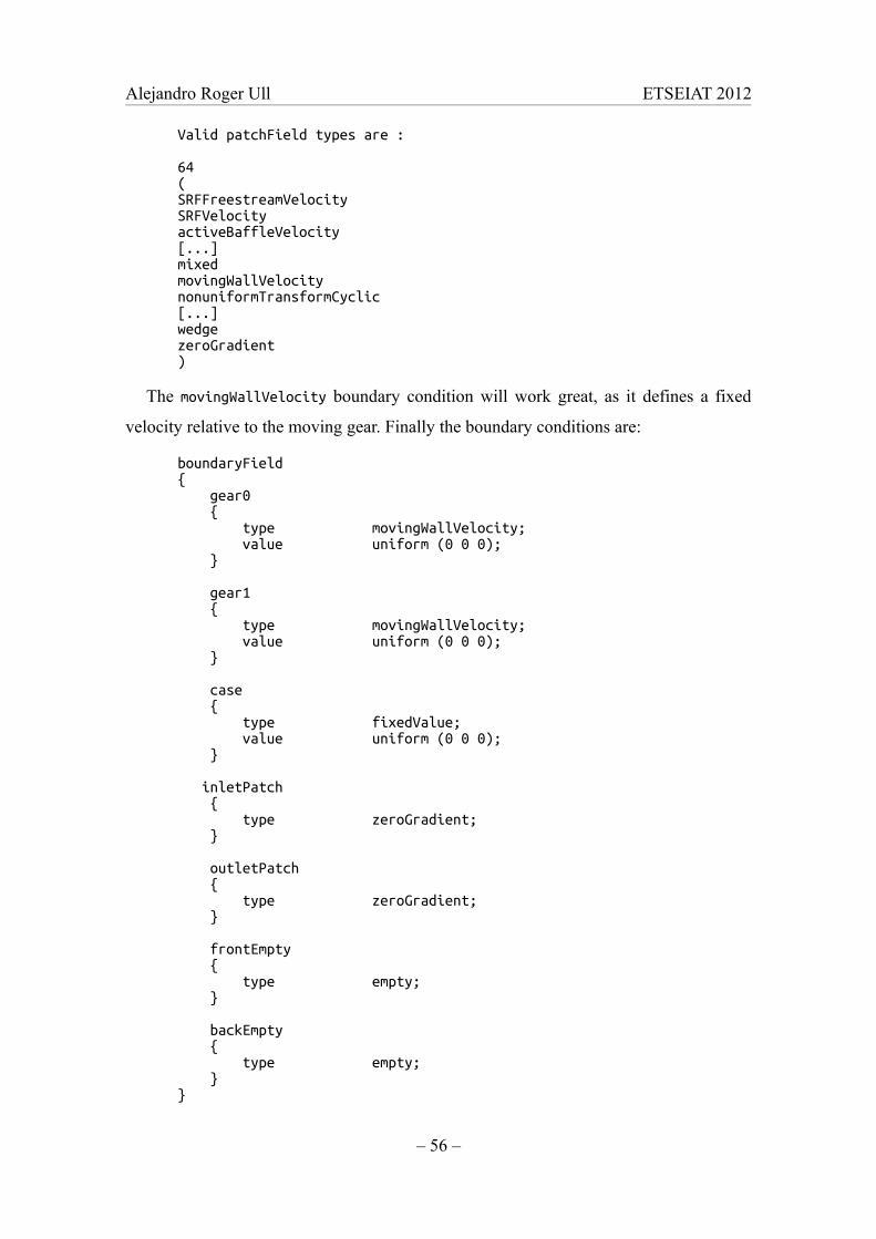
Valid patchField types are :
64 ( SRFFreestreamVelocity SRFVelocity activeBaffleVelocity [...]mixed movingWallVelocity nonuniformTransformCyclic [...]wedge zeroGradient )
The movingWallVelocity boundary condition will work great, as it defines a fixed
velocity relative to the moving gear. Finally the boundary conditions are:
boundaryField { gear0 { type movingWallVelocity; value uniform (0 0 0); }
gear1 { type movingWallVelocity; value uniform (0 0 0); }
case { type fixedValue; value uniform (0 0 0); }
inletPatch { type zeroGradient; }
outletPatch { type zeroGradient; }
frontEmpty { type empty; }
backEmpty { type empty; } }
– 56 –

Alejandro Roger Ull ETSEIAT 2012
For the motion of the points more things must be changed from the movingCone
tutorial, as explained by José Plácido Parra Viol in [2]. As it has been said, in that
tutorial the points of the cone surface are set to move horizontally. It is because of this
that in the 0 directory of that tutorial a file named pointMotionUx appears. This is
directly related to the dynamicMeshDict file inside the constant directory. For the
movingCone tutorial that file reads:
FoamFile { version 2.0; format ascii; class dictionary; location "constant"; object dynamicMeshDict; }
dynamicFvMesh dynamicMotionSolverFvMesh; motionSolverLibs ( "libfvMotionSolvers.so" ); solver velocityComponentLaplacian x; diffusivity directional ( 1 200 0 );
It can be seen that the solver entry is set to velocityComponentLaplacian x. For the
gears to rotate the motion of the points will have multiple components, so this solver is
not interesting. To find an interesting solver one can follow the same trial-and-error
strategy as before. By defining the solver as invented and trying to run the tutorial one
gets the following error:
--> FOAM FATAL ERROR: Unknown solver type invented
Valid solver types are:
7 ( displacementComponentLaplacian displacementInterpolation displacementLaplacian displacementLayeredMotion displacementSBRStress velocityComponentLaplacian velocityLaplacian )
It would be interesting to use the velocityLaplacian solver, similar to the one used
in the movingCone tutorial, but for all components of the velocity, not just one. In
addition to that, the diffusivity is modified so that both x and y directions have the same
value. Different diffusivity models can be applied, but before analyzing them the case
– 57 –

Alejandro Roger Ull ETSEIAT 2012
must be up and running. A basic analysis of the different diffusivity models for a cavity
with a rotating obstacle is done in [2]. The following entries in the dynamicMeshDict file
of the gearMove case are modified:
solver velocityLaplacian; diffusivity directional ( 1 1 0 );
Evidently, this velocityLaplacian solver requires a different boundary setup to that
of the velocityComponentLaplacian solver. By trying to run the movingCone tutorial
with the modified dynamicMeshDict file one gets an error explaining that the solver
expected to find a file called pointMotionU. It is because of this that the pointMotionUx
file inside the 0 directory is renamed as pointMotionU and modified to be a vector field
instead of the original scalar field. Thus, the header of the pointMotionU file reads:
FoamFile { version 2.0; format ascii; class pointVectorField; object pointMotionU; }
Note how the class entry is modified from pointScalarField to pointVectorField.
The dimensions are kept, and the value for the internal field now is a uniform vector:
dimensions [0 1 -1 0 0 0 0];
internalField uniform (0 0 0);
Again, to get the right boundary conditions for the gears the trial-and-error procedure
is followed. This time however, one finds that there is no boundary condition to enforce
a fixed angular velocity:
--> FOAM FATAL IO ERROR: Unknown patchField type invented for patch type wall
Valid patchField types are :
25( angularOscillatingDisplacement angularOscillatingVelocity calculated cyclic cyclicAMI cyclicSlip empty fixedNormalSlip fixedValue mixed
– 58 –
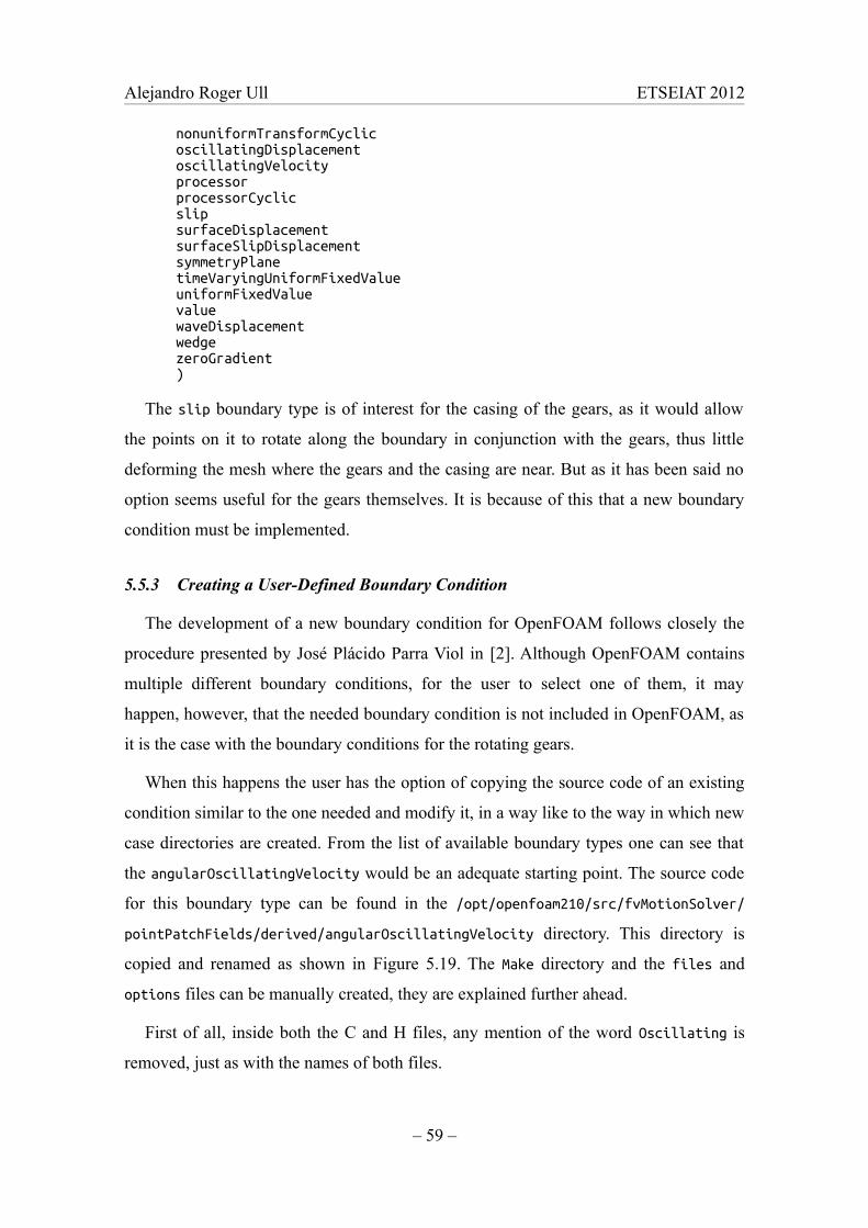
Alejandro Roger Ull ETSEIAT 2012
nonuniformTransformCyclic oscillatingDisplacement oscillatingVelocity processor processorCyclic slip surfaceDisplacement surfaceSlipDisplacement symmetryPlane timeVaryingUniformFixedValue uniformFixedValue value waveDisplacement wedge zeroGradient )
The slip boundary type is of interest for the casing of the gears, as it would allow
the points on it to rotate along the boundary in conjunction with the gears, thus little
deforming the mesh where the gears and the casing are near. But as it has been said no
option seems useful for the gears themselves. It is because of this that a new boundary
condition must be implemented.
5.5.3 Creating a User-Defined Boundary Condition
The development of a new boundary condition for OpenFOAM follows closely the
procedure presented by José Plácido Parra Viol in [2]. Although OpenFOAM contains
multiple different boundary conditions, for the user to select one of them, it may
happen, however, that the needed boundary condition is not included in OpenFOAM, as
it is the case with the boundary conditions for the rotating gears.
When this happens the user has the option of copying the source code of an existing
condition similar to the one needed and modify it, in a way like to the way in which new
case directories are created. From the list of available boundary types one can see that
the angularOscillatingVelocity would be an adequate starting point. The source code
for this boundary type can be found in the /opt/openfoam210/src/fvMotionSolver/
pointPatchFields/derived/angularOscillatingVelocity directory. This directory is
copied and renamed as shown in Figure 5.19. The Make directory and the files and
options files can be manually created, they are explained further ahead.
First of all, inside both the C and H files, any mention of the word Oscillating is
removed, just as with the names of both files.
– 59 –
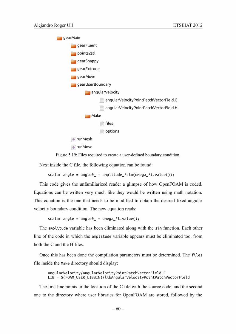
Alejandro Roger Ull ETSEIAT 2012
gearMain
gearFluent
points2stl
gearSnappy
gearExtrude
gearMove
gearUserBoundary
angularVelocity
angularVelocityPointPatchVectorField.C
angularVelocityPointPatchVectorField.H
Make
files
options
runMesh
runMove
Figure 5.19: Files required to create a user-defined boundary condition.
Next inside the C file, the following equation can be found:
scalar angle = angle0_ + amplitude_*sin(omega_*t.value());
This code gives the unfamiliarized reader a glimpse of how OpenFOAM is coded.
Equations can be written very much like they would be written using math notation.
This equation is the one that needs to be modified to obtain the desired fixed angular
velocity boundary condition. The new equation reads:
scalar angle = angle0_ + omega_*t.value();
The amplitude variable has been eliminated along with the sin function. Each other
line of the code in which the amplitude variable appears must be eliminated too, from
both the C and the H files.
Once this has been done the compilation parameters must be determined. The files
file inside the Make directory should display:
angularVelocity/angularVelocityPointPatchVectorField.C LIB = $(FOAM_USER_LIBBIN)/libAngularVelocityPointPatchVectorField
The first line points to the location of the C file with the source code, and the second
one to the directory where user libraries for OpenFOAM are stored, followed by the
– 60 –
Alejandro Roger Ull ETSEIAT 2012
name of the library that will be created. The directory is stored in the
$FOAM_USER_LIBBIN variable, and can be easily retrieved by typing at the terminal:
echo $FOAM_USER_LIBBIN
The options file is in charge of pointing to the directory in which the included H
files from OpenFOAM are located, and to load the required libraries.
EXE_INC = \ -I$(LIB_SRC)/finiteVolume/lnInclude LIB_LIBS = \ -lfiniteVolume
Once all the files are correctly setup the user-defined boundary condition can be
compiled by changing to the folder in which the files where stored, gearUserBoundary
in this case, and running:
wmake libso
If the output displays at the end a message like:
'/home/userName/OpenFOAM/userName-2.1.0/platforms/linux64GccDPOpt/ lib/libAngularVelocityPointPatchVectorField.so' is up to date.
Then the user-defined boundary condition library has been correctly compiled. In
order to be able to use it, the following line will be added to the controlDict file:
libs ("libAngularVelocityPointPatchVectorField.so" "libOpenFOAM.so")
Once the library is available the trial-and-error message will list it as a valid option
when trying to run the code with the invented boundary condition again.
--> FOAM FATAL IO ERROR: Unknown patchField type invented for patch type wall
Valid patchField types are :
26( angularOscillatingDisplacement angularOscillatingVelocity angularVelocitycalculated cyclic
[...]
zeroGradient)
Now the pointMotionU file can have the boundaryField dictionary completed:
– 61 –
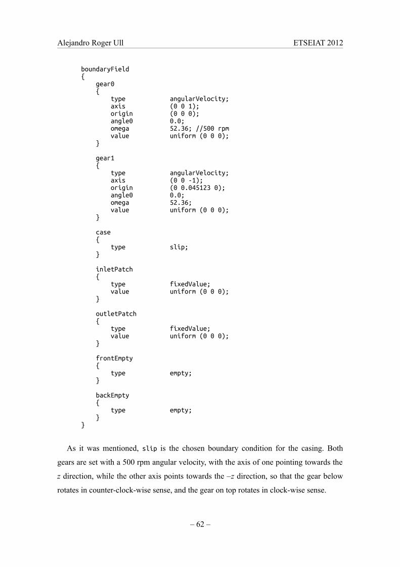
Alejandro Roger Ull ETSEIAT 2012
boundaryField { gear0 { type angularVelocity; axis (0 0 1); origin (0 0 0); angle0 0.0; omega 52.36; //500 rpm value uniform (0 0 0); }
gear1 { type angularVelocity; axis (0 0 -1); origin (0 0.045123 0); angle0 0.0; omega 52.36; value uniform (0 0 0); }
case { type slip; }
inletPatch { type fixedValue; value uniform (0 0 0); }
outletPatch { type fixedValue; value uniform (0 0 0); }
frontEmpty { type empty; }
backEmpty { type empty; } }
As it was mentioned, slip is the chosen boundary condition for the casing. Both
gears are set with a 500 rpm angular velocity, with the axis of one pointing towards the
z direction, while the other axis points towards the –z direction, so that the gear below
rotates in counter-clock-wise sense, and the gear on top rotates in clock-wise sense.
– 62 –
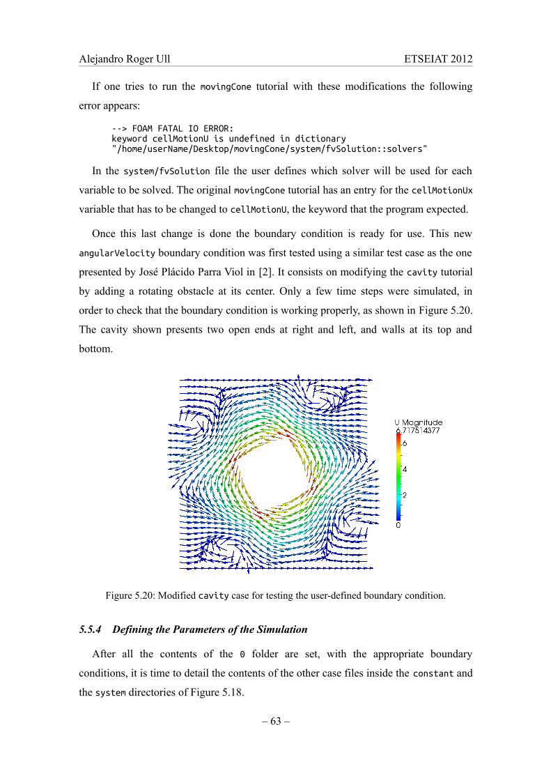
Alejandro Roger Ull ETSEIAT 2012
If one tries to run the movingCone tutorial with these modifications the following
error appears:
--> FOAM FATAL IO ERROR: keyword cellMotionU is undefined in dictionary "/home/userName/Desktop/movingCone/system/fvSolution::solvers"
In the system/fvSolution file the user defines which solver will be used for each
variable to be solved. The original movingCone tutorial has an entry for the cellMotionUx
variable that has to be changed to cellMotionU, the keyword that the program expected.
Once this last change is done the boundary condition is ready for use. This new
angularVelocity boundary condition was first tested using a similar test case as the one
presented by José Plácido Parra Viol in [2]. It consists on modifying the cavity tutorial
by adding a rotating obstacle at its center. Only a few time steps were simulated, in
order to check that the boundary condition is working properly, as shown in Figure 5.20.
The cavity shown presents two open ends at right and left, and walls at its top and
bottom.
Figure 5.20: Modified cavity case for testing the user-defined boundary condition.
5.5.4 Defining the Parameters of the Simulation
After all the contents of the 0 folder are set, with the appropriate boundary
conditions, it is time to detail the contents of the other case files inside the constant and
the system directories of Figure 5.18.
– 63 –

Alejandro Roger Ull ETSEIAT 2012
Inside the constant directory there is a polyMesh directory that will contain the mesh
generated with the runMesh script. The contents of the dynamicMeshDict file have
already been discussed while developing the user-defined boundary condition in the
previous section. The transportProperties file reads:
transportModel Newtonian;
nu nu [ 0 2 -1 0 0 0 0 ] 3.164e-05;
Where the nu field shows the kinematic viscosity obtained from [1].
As it was mentioned, for this study the simulation is set to laminar. Because of this
the turbulenceProperties file has only the following entry:
simulationType laminar;
Obviously this can be modified if turbulence is going to be simulated. Once the
parameters in the constant directory have been determined it is time to set the
dictionaries in the system directory. The controlDict file is modified to include an
external file called timeDict, in order to make some time controls easier to modify later:
#include "timeDict"
libs ("libAngularVelocityPointPatchVectorField.so" "libOpenFOAM.so")
application pimpleDyMFoam;
startFrom startTime; startTime $start;
stopAt endTime; endTime $end;
deltaT $delta;
writeControl timeStep; writeInterval $write;
purgeWrite 0;
writeFormat binary; writePrecision 6; writeCompression off;
timeFormat general; timePrecision 6;
runTimeModifiable true;
adjustTimeStep no; maxCo 0.5;
– 64 –
Alejandro Roger Ull ETSEIAT 2012
As it can be seen, the startTime, endTime, deltaT and writeInterval entries are read
from the start, end, delta and write variables respectively. Those variables are defined
in the included dictionary timeDict as shown:
start 0; end 1e-3; delta 1e-5; write 10; #inputMode merge
These sample values will be changed later on. This kind of file connection with the
#include instruction is particularly useful when some parameters are going to be
changed frequently, or in a lot of places at the same time, so that these changes can be
quickly performed on a single file.
The decomposeParDict file can be kept from the gearSnappy case directory. The
complexity of the case makes it a good idea to run the code in parallel. Also, this was
one of the main justifications of this study: to be able to freely run the CFD solver in
parallel with no worries for licensing restrictions.
The fvSchemes and fvSolution files can be directly copied from the movingCone
tutorial, with the mentioned change of renaming the cellMotionUx entry to cellMotionU
in the fvSolution file.
In the fvSchemes file the user is able to specify which numerical scheme is used for
calculating time derivatives, gradients, divergences, laplacians and interpolations,
among other things. On the other hand, as mentioned, in the fvSolution file the user
specifies the different solvers that are going to be used to solve for the different
variables, with their corresponding parameters such as relaxation factors. These two
files are another glimpse at the power of customization OpenFOAM offers to the user.
After all the parameters have been set, the case is ready to run.
5.5.5 Running the Moving Gear
Before writing a script to automate the run process, it is interesting to run the case
manually and check for all the possible problems that may arise. The first step to run the
case manually is to decompose the domain the same way that was done with
snappyHexMesh, by using the decomposePar tool. In theory this process poses no
problem, but when trying to run the pimpleDyMFoam solver in parallel by typing:
– 65 –
Alejandro Roger Ull ETSEIAT 2012
foamJob -s -p pimpleDyMFoam
The following error is found, once per processor:
--> FOAM FATAL IO ERROR: size 10270 is not equal to the given value of 2376
file: /home/userName/Desktop/gearMain/gearMove/processor0/0/pointMotionU:: boundaryField::gear0 from line 46 to line 54.
By manually inspecting the pointMotionU file located inside one of the processor’s 0
directory one finds that the uniform boundary conditions on gears has been substituted
by a nonuniform List<vector> entry. If the write mode is set to ascii in the
controlDict file, one can see that the processor0/0/pointMotionU shows:
gear0 { type angularVelocity; axis (0 0 1); origin (0 0 0); angle0 0; omega 52.36; p0 nonuniform List<vector> 10270 ( (-0.0214975 -0.00630927 0) [...])
But the list is incorrectly generated. This is because the decomposePar tool doesn’t
handle correctly the user-defined boundary conditions, as explained by José Plácido
Parra Viol in [2]. Further examining the file one notes the following additional
processor patches and boundary conditions, such as:
procBoundary0to4 { type processor; }
These additional patches are created to keep the different processors connected.
Additionally, some patches are specified as a list of 0 length, for example:
outletPatch { type fixedValue; value nonuniform 0(); }
This is because that patch is on a different processor or processors, so no value has to
be applied to any point in that processor.
– 66 –

Alejandro Roger Ull ETSEIAT 2012
After inspecting the pointMotionU file of the processor directories it can be
concluded that the problem might be solved by substituting the decomposed
pointMotionU files with the original one inside the 0 directory. The badly defined
angularVelocity boundary conditions would be fixed, and the patches with no points in
a processor would not cause any problem if specified as uniform, since the problem is
caused by specifying boundaries with incorrect point lists. A uniform boundary
condition would not be applied to any point if the processor has no points in that patch.
However, in order to be able to replace the generated files with the original one, the
boundary conditions for each processor patch would need to be manually created.
Fortunately there is an easy way of creating a boundary condition definition for
multiple, similarly-named patches in no time by using wildcards.
OpenFOAM uses what are called regular expressions. One can define such an
expression by using strings enclosed in quotes “...”. As explained in [5], the following
wildcards are allowed, among others:
Card Definition
. Matches any character
( ) Groups a series of characters
[ ] Denotes a set of character matches
* Matches the preceding character 0 or more times
+ Matches the preceding character 1 or more times
? Matches the preceding character 0 or 1 times
| Denotes alternate possibilities (OR)
$ End of line
^ Beginning of line. Also a NOT if whithin [ ].
Table 5.2: Examples of wildcards allowed in regular expressions.
Since one knows the naming pattern for the processor patches, the following entry
can be added to the original pointMotionU file inside the 0 directory:
"procBoundary.*" { type processor; }
This way the processor boundary type is applied to any patch whose name begins by
procBoundary and is followed by any number of any characters, as specified by the dot
followed by the star at the end of the regular expression.
– 67 –
Alejandro Roger Ull ETSEIAT 2012
With this addition to the pointMotionU file inside the 0 directory, it can now replace
the corresponding files inside the processor directories. Now the foamJob command can
be launched and the simulation starts. But the complete flow simulation requires a small
time step, making the calculations longer. It is because of this that another command is
will be used:
foamJob -s -p moveMesh
With the moveMesh command only the mesh movement is calculated; flow variables
are not taken into account. This way the maximum acceptable deformation of the mesh
can be determined quicker than with pimpleDyMFoam.
After running the simulation the domain must be reconstructed again. This can be
done in this case by running the reconstructPar tool. But when trying to run it another
problem appears:
Reconstructing point fields
Reconstructing pointVectorFields
pointMotionU *** glibc detected *** reconstructPar: malloc(): memory corruption: 0x0000000006278f80 ***
The reconstruction of the pointMotionU file fails. But the problem can be easily
solved by removing all the pointMotionU files from inside the processor directories
after the simulation takes place, as they are no longer needed. The fields of interest are
the pressure p and the velocity U. After removing them the reconstructPar command
works without any error showing up.
5.5.6 runMove
As with the meshing, the instructions needed to run the case are gathered inside a
single bash script, so that all the required steps can be performed with a single
command. As shown in Figure 5.18 the runMove script is located inside the gearMain
folder, along with the runMesh bash script.
The runMesh code is described next. First the OpenFOAM commands are loaded. The
script moves to the gearMove directory and decomposes the domain. Then for each
processor directory the pointMotionU file is copied to that directory, overwriting the file
that was decomposed incorrectly. After that the mesh is renumbered, as during the
– 68 –

Alejandro Roger Ull ETSEIAT 2012
meshing procedure, although this step is not completely necessary. Finally all the
pointMotionU files inside all the processor directories are removed, prior to
reconstructing the mesh. After the mesh has been reconstructed the processor
directories and the log file can be deleted.
So the runMesh bash script code is finally:
#!/bin/bash
. /opt/openfoam210/etc/bashrc
cd gearMove/
# Decompose and copy pointMotionU decomposePar
for dir in $( ls | grep "processor" ) do cp 0/pointMotionU $dir/0/pointMotionU done
# Run solver foamJob -s -p renumberMesh -overwrite foamJob -s -p moveMesh
# Delete all pointMotionU and Reconstruct rm processor*/*/pointMotionU reconstructPar rm -rf log processor*
5.5.7 Testing the Limits of the Mesh
After running the above script and visually examining the results, which are shown
on Figure 5.21, one can easily see that it is at the corners of the casing that the mesh is
deformed the most, while the space between two consecutive teeth of the gears and the
casing does not deform at all, since the points on the casing are allowed to slip while the
gears rotate.
Also, the checkMesh utility can be used to check the different meshes for errors. Only
three kinds of errors appear on the meshes, but their severity is increased with the
rotation of the mesh as expected. Results are shown on Table 5.3.
The limit to the number of errors in the mesh that one can allow to himself highly
depends on the purpose of the calculations and the desired accuracy and precision. For
this study, with the main purpose of developing methods and procedures to work with
dynamic meshes, the limit is set to 0.0002 s, at least at this point, but for any other
purpose the user will need to select a proper limit for his or her study.
– 69 –
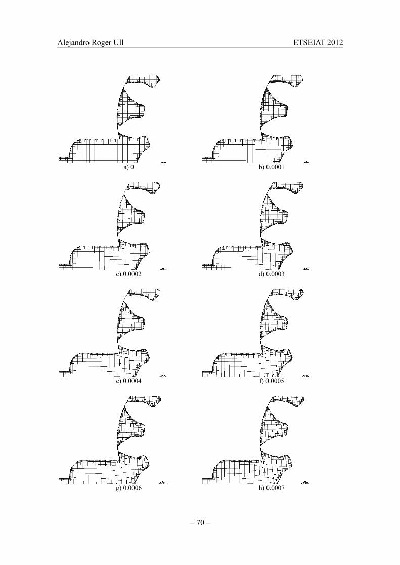
Alejandro Roger Ull ETSEIAT 2012
a) 0 b) 0.0001
c) 0.0002 d) 0.0003
e) 0.0004 f) 0.0005
g) 0.0006 h) 0.0007
– 70 –

Alejandro Roger Ull ETSEIAT 2012
i) 0.0008 j) 0.0009
Figure 5.21: Deformation of the initial mesh with moveMesh.
Time (s)Non-orthogonal faces
Incorrectly oriented faces
Highly skewed faces
0 0 0 1
0.0001 0 31 2
0.0002 5 27 7
0.0003 16 44 7
0.0004 34 64 15
0.0005 67 79 11
0.0006 136 142 18
0.0007 211 207 23
0.0008 372 307 44
0.0009 546 395 53
0.0010 772 479 74
Table 5.3: Results of the checkMesh tool for the deformed meshes.
5.6 Performing a Complete Gearing Cycle
Once the limit of the deformation has been determined it is time to move the mesh
through a complete gearing cycle of the pump. The idea is to start with the initial mesh,
deform it until the limit that has just been set, and then replace the mesh with a new one.
This process can be repeated until a complete gearing cycle has been performed.
Indeed, after a gearing cycle the user will probably desire to perform another cycle,
and so on, until the convergence criteria is met. Because of this, the different base
meshes will be created firstly, and then the deformation and substitution will take place.
– 71 –
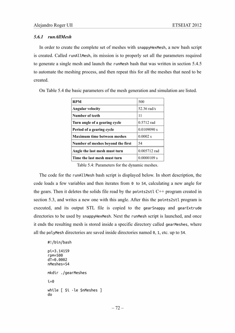
Alejandro Roger Ull ETSEIAT 2012
5.6.1 runAllMesh
In order to create the complete set of meshes with snappyHexMesh, a new bash script
is created. Called runAllMesh, its mission is to properly set all the parameters required
to generate a single mesh and launch the runMesh bash that was written in section 5.4.5
to automate the meshing process, and then repeat this for all the meshes that need to be
created.
On Table 5.4 the basic parameters of the mesh generation and simulation are listed.
RPM 500
Angular velocity 52.36 rad/s
Number of teeth 11
Turn angle of a gearing cycle 0.5712 rad
Period of a gearing cycle 0.0109090 s
Maximum time between meshes 0.0002 s
Number of meshes beyond the first 54
Angle the last mesh must turn 0.005712 rad
Time the last mesh must turn 0.0000109 s
Table 5.4: Parameters for the dynamic meshes.
The code for the runAllMesh bash script is displayed below. In short description, the
code loads a few variables and then iterates from 0 to 54, calculating a new angle for
the gears. Then it deletes the solids file read by the points2stl C++ program created in
section 5.3, and writes a new one with this angle. After this the points2stl program is
executed, and its output STL file is copied to the gearSnappy and gearExtrude
directories to be used by snappyHexMesh. Next the runMesh script is launched, and once
it ends the resulting mesh is stored inside a specific directory called gearMeshes, where
all the polyMesh directories are saved inside directories named 0, 1, etc. up to 54.
#!/bin/bash
pi=3.14159 rpm=500 dT=0.0002 nMeshes=54
mkdir ./gearMeshes
i=0
while [ $i -le $nMeshes ] do
– 72 –
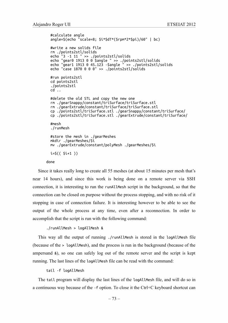
Alejandro Roger Ull ETSEIAT 2012
#calculate angle angle=$(echo "scale=8; $i*$dT*($rpm*2*$pi)/60" | bc) #write a new solids file rm ./points2stl/solids echo "3 -1 11 " >> ./points2stl/solids echo "gear0 1913 0 0 $angle " >> ./points2stl/solids echo "gear1 1913 0 45.123 -$angle " >> ./points2stl/solids echo "case 1870 0 0 0" >> ./points2stl/solids #run points2stl cd points2stl ./points2stl cd ..
#delete the old STL and copy the new one rm ./gearSnappy/constant/triSurface/triSurface.stl rm ./gearExtrude/constant/triSurface/triSurface.stl cp ./points2stl/triSurface.stl ./gearSnappy/constant/triSurface/ cp ./points2stl/triSurface.stl ./gearExtrude/constant/triSurface/
#mesh ./runMesh
#store the mesh in ./gearMeshes mkdir ./gearMeshes/$i mv ./gearExtrude/constant/polyMesh ./gearMeshes/$i
i=$(( $i+1 ))
done
Since it takes really long to create all 55 meshes (at about 15 minutes per mesh that’s
near 14 hours), and since this work is being done on a remote server via SSH
connection, it is interesting to run the runAllMesh script in the background, so that the
connection can be closed on purpose without the process stopping, and with no risk of it
stopping in case of connection failure. It is interesting however to be able to see the
output of the whole process at any time, even after a reconnection. In order to
accomplish that the script is run with the following command:
./runAllMesh > logAllMesh &
This way all the output of running ./runAllMesh is stored in the logAllMesh file
(because of the > logAllMesh), and the process is run in the background (because of the
ampersand &), so one can safely log out of the remote server and the script is kept
running. The last lines of the logAllMesh file can be read with the command:
tail -f logAllMesh
The tail program will display the last lines of the logAllMesh file, and will do so in
a continuous way because of the -f option. To close it the Ctrl+C keyboard shortcut can
– 73 –
Alejandro Roger Ull ETSEIAT 2012
be used, it will kill most foreground running programs. But if the user wants to kill the
running script, since it is running in the background, it must be killed with the pkill
command:
pkill runAllMesh
This will kill the script, but not the last application run with it, which most of the
time is snappyHexMesh, although this can be checked with the top utility. The running
application must be killed separately.
Some of the meshes created with the runAllMesh script are shown in Figure 5.22:
a) Mesh 0. b) Mesh 0. Detail.
c) Mesh 13. d) Mesh 13. Detail.
e) Mesh 27. f) Mesh 27. Detail.
– 74 –
Alejandro Roger Ull ETSEIAT 2012
g) Mesh 40. h) Mesh 40. Detail.
i) Mesh 54. j) Mesh 54. Detail.
Figure 5.22: Meshes generated with runAllMesh.
It has some interest to note that, since the same blockMesh background mesh and the
same snappyHexMesh parameters are being used for all meshes, most points of the mesh
do not change. It is said by David del Campo Sud in [1] that the simulation of cavitation
was badly affected by interpolation errors produced each time the mesh was
regenerated.
Although it could be very expensive in terms of time, in the future it could be studied
if it is possible to run a simulation consisting of only generated meshes, without
deforming the mesh. This way interpolation would be very localized, only very near the
gears, and maybe cavitation simulations are not negatively affected.
5.6.2 runAllMove
After all the base meshes have been created with the help of the runAllMesh bash
script, now another script is created, named runAllMove. Similarly to the runAllMesh,
this script will perform a loop in which the parameters for the runMove script are set to
their appropriate values for each iteration, an then the runMove script is run. After each
iteration some representative meshes are stored.
– 75 –
Alejandro Roger Ull ETSEIAT 2012
#!/bin/bash
deltaT=2e-6 endTime=0.0002 writeSteps=25 endLast=.000108 writeLast=27 nMeshes=54 nCycles=1 mkdir gearResults
i=1 while [ $i -le $nCycles ] do j=0 while [ $j -le $nMeshes ] do cp -rf gearMoveCopy/* gearMove/ cp -rf gearMeshes/$j/polyMesh/ gearMove/constant
if [ $j != $nMeshes ] then rm gearMove/system/timeDict echo "start 0;" >> gearMove/system/timeDict echo "end "$endTime";" >> gearMove/system/timeDict echo "delta "$deltaT";" >> gearMove/system/timeDict echo "write "$writeSteps";" >> gearMove/system/timeDict echo "#inputMode merge" >> gearMove/system/timeDict elif [ $j = $nMeshes ] then rm gearMove/system/timeDict echo "start 0;" >> gearMove/system/timeDict echo "end "$endLast";" >> gearMove/system/timeDict echo "delta "$deltaT";" >> gearMove/system/timeDict echo "write "$writeLast";" >> gearMove/system/timeDict echo "#inputMode merge" >> gearMove/system/timeDict fi
./runMove
if [ $i = $nCycles ] then rm -rf gearMove/{0,constant,system,log} if [ $j != $nMeshes ] then cp -rf gearMove/5e-05 gearResults/$j.1 cp -rf gearMove/0.0001 gearResults/$j.2 cp -rf gearMove/0.00015 gearResults/$j.3 cp -rf gearMove/0.0002 gearResults/$j.4 else cp -rf gearMove/5.4e-05 gearResults/$j.1 cp -rf gearMove/0.000108 gearResults/$j.2 fi rm -rf gearMove/* fi
j=$(( $j+1 )) done i=$(( $i+1 )) done
– 76 –
Alejandro Roger Ull ETSEIAT 2012
Before the script is run a copy of all the contents of the gearMove directory are stored
in a backup copy at gearMoveCopy. Then, when each iteration starts, the gearMove
directory is cleared and the backup is restored, so that each runMove starts with a clean
configuration.
Note how the parameters that are stored in the timeDict file change for the last mesh
iteration, according with Table 5.4. Also, the meshes are stored somehow manually,
since the names of the folders to be copied are hard coded in the script.
It is important to keep in mind that all the simulations must begin at time 0 s,
otherwise the gears would rotate to match their position with the starting time. For
instance, if the second iteration were to start at time 1 s, the mesh would rotate 52.36 rad
before that simulation ever begins, rolling the mesh around both gears and rendering it
completely unusable.
After running the runAllMove script the results are quite satisfactory. Results can be
seen in the animations that are in the media given with this work.
5.6.3 runPimple & runAllPimple
It must be noted too that the above script is conceived for moving the mesh
exclusively, with the moveMesh command no flow is being calculated. The runAllMove
script does consider an important point for a flow simulation, since it is able to run for
multiple gearing cycles before writing the results of the last one. But to be able to
simulate the complete flow a last step is needed: the flow results must be interpolated
from one mesh to the next one.
In the first place, the runMove script can be quickly modified to execute the
pimpleDyMFoam application instead of the moveMesh application. With that easy change
the new script can be saved as runPimple.
Next the runAllMove bash script is copied as runAllPimple, since the base of the
script will be the same. After that, the mapFields utility must be added to the
runAllPimple script. This utility is explained in the cavity tutorial presented in [3]. In
short, it requires the user to specify the source case from which the results are going to
be interpolated. The fields from the starting time specified in the controlDict of the
target case are mapped onto it.
– 77 –
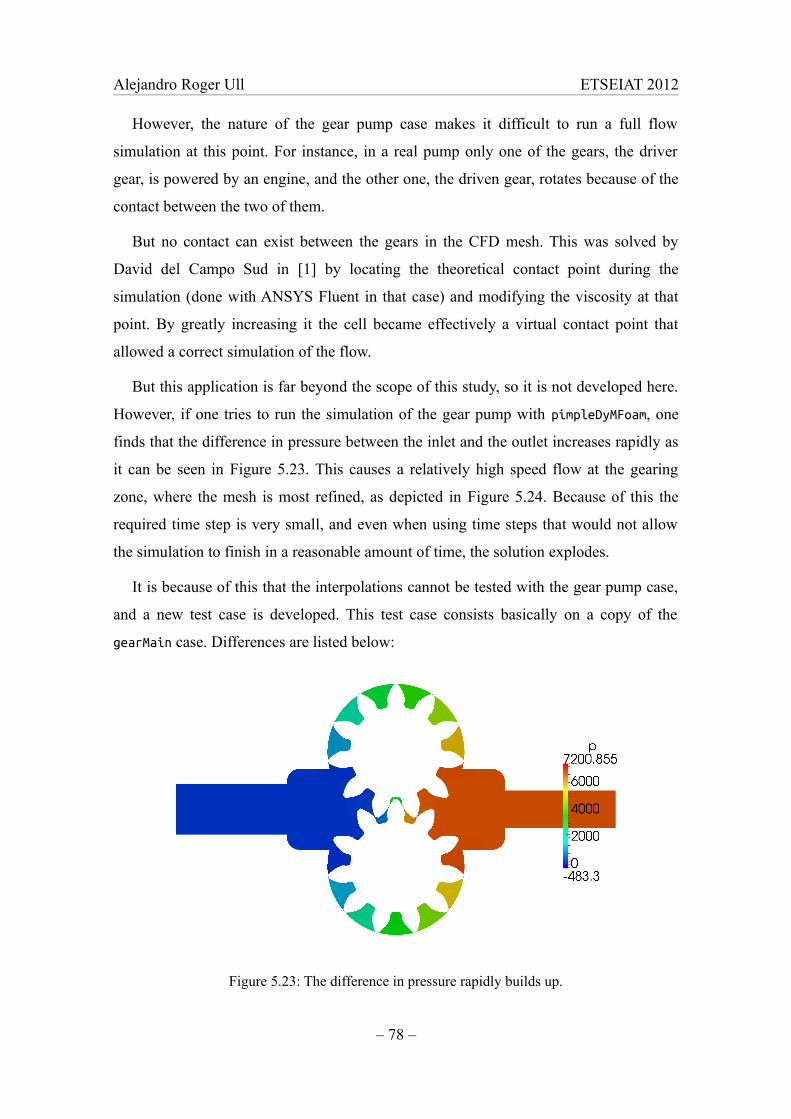
Alejandro Roger Ull ETSEIAT 2012
However, the nature of the gear pump case makes it difficult to run a full flow
simulation at this point. For instance, in a real pump only one of the gears, the driver
gear, is powered by an engine, and the other one, the driven gear, rotates because of the
contact between the two of them.
But no contact can exist between the gears in the CFD mesh. This was solved by
David del Campo Sud in [1] by locating the theoretical contact point during the
simulation (done with ANSYS Fluent in that case) and modifying the viscosity at that
point. By greatly increasing it the cell became effectively a virtual contact point that
allowed a correct simulation of the flow.
But this application is far beyond the scope of this study, so it is not developed here.
However, if one tries to run the simulation of the gear pump with pimpleDyMFoam, one
finds that the difference in pressure between the inlet and the outlet increases rapidly as
it can be seen in Figure 5.23. This causes a relatively high speed flow at the gearing
zone, where the mesh is most refined, as depicted in Figure 5.24. Because of this the
required time step is very small, and even when using time steps that would not allow
the simulation to finish in a reasonable amount of time, the solution explodes.
It is because of this that the interpolations cannot be tested with the gear pump case,
and a new test case is developed. This test case consists basically on a copy of the
gearMain case. Differences are listed below:
Figure 5.23: The difference in pressure rapidly builds up.
– 78 –
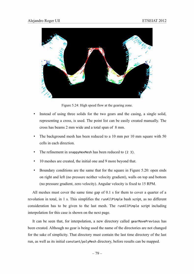
Alejandro Roger Ull ETSEIAT 2012
Figure 5.24: High speed flow at the gearing zone.
• Instead of using three solids for the two gears and the casing, a single solid,
representing a cross, is used. The point list can be easily created manually. The
cross has beams 2 mm wide and a total span of 8 mm.
• The background mesh has been reduced to a 10 mm per 10 mm square with 50
cells in each direction.
• The refinement in snappyHexMesh has been reduced to (2 3).
• 10 meshes are created, the initial one and 9 more beyond that.
• Boundary conditions are the same that for the square in Figure 5.20: open ends
on right and left (no pressure neither velocity gradient), walls on top and bottom
(no pressure gradient, zero velocity). Angular velocity is fixed to 15 RPM.
All meshes must cover the same time gap of 0.1 s for them to cover a quarter of a
revolution in total, in 1 s. This simplifies the runAllPimple bash script, as no different
consideration has to be given to the last mesh. The runAllPimple script including
interpolation for this case is shown on the next page.
It can be seen that, for interpolation, a new directory called gearMovePrevious has
been created. Although no gear is being used the name of the directories are not changed
for the sake of simplicity. That directory must contain the last time directory of the last
run, as well as its initial constant/polyMesh directory, before results can be mapped.
– 79 –

Alejandro Roger Ull ETSEIAT 2012
#!/bin/bash
deltaT=0.00004 endTime=0.1 writeSteps=1250 nMeshes=9nCycles=5 mkdir gearResults
i=1 while [ $i -le $nCycles ]do j=0 while [ $j -le $nMeshes ] do rm -rf gearMove/* cp -rf gearMoveCopy/* gearMove/ cp -rf gearMeshes/$j/polyMesh/ gearMove/constant
rm gearMove/system/timeDict echo "start 0;" >> gearMove/system/timeDict echo "end "$endTime";" >> gearMove/system/timeDict echo "delta "$deltaT";" >> gearMove/system/timeDict echo "write "$writeSteps";" >> gearMove/system/timeDict echo "#inputMode merge" >> gearMove/system/timeDict
if [ $j = 0 ] && [ $i = 1 ] then cd . #do not interpolate on first run else cd gearMove mapFields ../gearMovePrevious -sourceTime latestTime cd .. cp -rf gearMoveCopy/0/pointMotionU gearMove/0/pointMotionU fi
./runPimple
mkdir gearMovePrevious/0 rm -rf gearMovePrevious/0/* rm -rf gearMovePrevious/constant/polyMesh/*
cp -rf gearMove/0.1/* gearMovePrevious/0/ cp -rf gearMove/constant/polyMesh/* gearMovePrevious/constant/polyMesh
if [ $i = $nCycles ] then rm -rf gearMove/{constant,system,log}
cp -rf gearMove/0 gearResults/$j cp -rf gearMove/0.05 gearResults/$j.1 cp -rf gearMove/0.1 gearResults/$j.2
rm -rf gearMove/* fi
j=$(( $j+1 )) done i=$(( $i+1 )) done
– 80 –
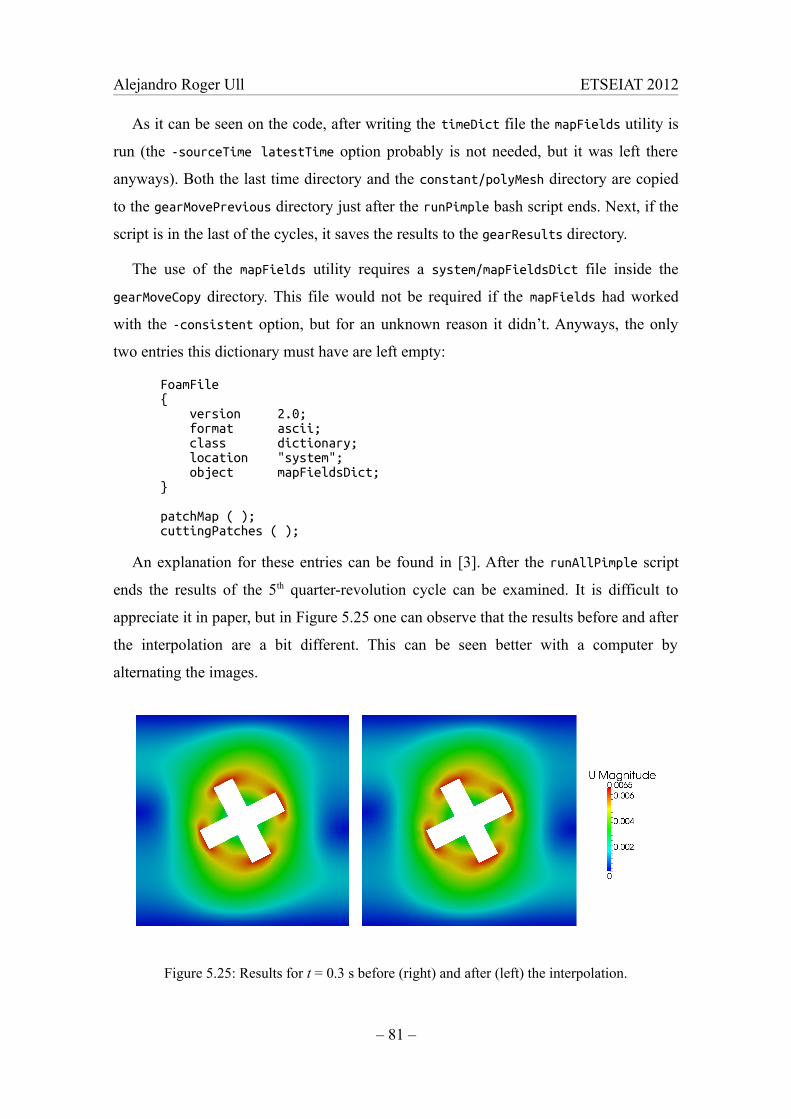
Alejandro Roger Ull ETSEIAT 2012
As it can be seen on the code, after writing the timeDict file the mapFields utility is
run (the -sourceTime latestTime option probably is not needed, but it was left there
anyways). Both the last time directory and the constant/polyMesh directory are copied
to the gearMovePrevious directory just after the runPimple bash script ends. Next, if the
script is in the last of the cycles, it saves the results to the gearResults directory.
The use of the mapFields utility requires a system/mapFieldsDict file inside the
gearMoveCopy directory. This file would not be required if the mapFields had worked
with the -consistent option, but for an unknown reason it didn’t. Anyways, the only
two entries this dictionary must have are left empty:
FoamFile { version 2.0; format ascii; class dictionary; location "system"; object mapFieldsDict; }
patchMap ( ); cuttingPatches ( );
An explanation for these entries can be found in [3]. After the runAllPimple script
ends the results of the 5th quarter-revolution cycle can be examined. It is difficult to
appreciate it in paper, but in Figure 5.25 one can observe that the results before and after
the interpolation are a bit different. This can be seen better with a computer by
alternating the images.
Figure 5.25: Results for t = 0.3 s before (right) and after (left) the interpolation.
– 81 –
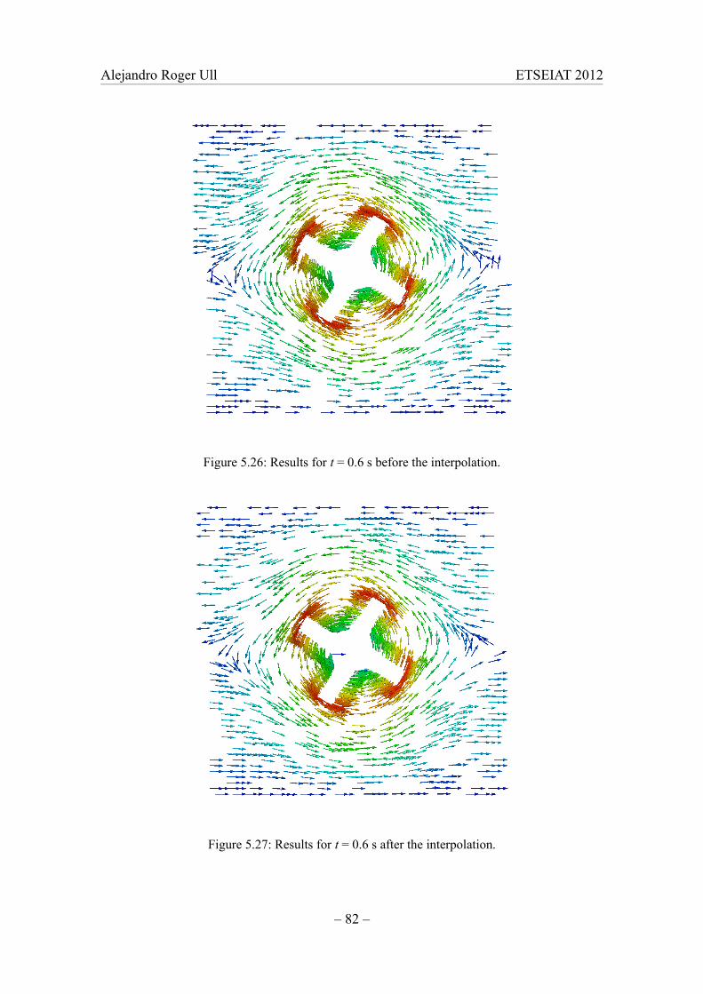
Alejandro Roger Ull ETSEIAT 2012
Figure 5.26: Results for t = 0.6 s before the interpolation.
Figure 5.27: Results for t = 0.6 s after the interpolation.
– 82 –

Alejandro Roger Ull ETSEIAT 2012
Figure 5.28: Deformed (right) and regenerated (left) meshes for t = 0.3 s.
This difference on the results before and after the interpolation are more visible on
Figure 5.26 when compared with Figure 5.27, where a pair of horizontal, no-velocity
arrows have appeared in the rotating cross wall. This can be due to interpolation failing
in a few points, at which the initial value of velocity has been left. Also, it can be seen in
Figure 5.28 the regeneration of the mesh.
In overall, the results of the runAllPimple script are satisfactory. It must be
remembered, though, that the interpolation errors where crucial when dealing with
cavitation simulations. But, nevertheless, the main purpose of this study is not to study
cavitation, but to provide a procedure to work with dynamic meshes in OpenFOAM.
– 83 –

Alejandro Roger Ull ETSEIAT 2012
6 RESULTS AND CONCLUSIONS
6.1 Results of This Study
The complete procedure developed in the previous section is qualitatively
summarized here, step by step:
1. A geometry for the gears and the casing has been obtained, in the form of a list
of points, from a provided Gambit MSH file. This geometry can be obtained
from other sources, but the target stays the same: to obtain a separate list of
points for each boundary of the gear pump domain, or for any other problem the
user may wish to solve.
2. A C++ program has been developed to convert a group of solids, defined by lists
of two-dimensional points, to an STL surface. Again, this STL surface can be
obtained with other methods, typically any CAD software is able to export to
this format, but the point here is that the C++ program developed here is able to
quickly modify the geometry in an automated way, as it is done in this study
with the rotation of the gears.
3. The parameters for meshing the obtained STL surface with snappyHexMesh in
parallel have been determined, and a script to automatically obtain a single mesh
has been written. The quality of the obtained mesh depends highly on these
parameters, as well as the time required to generate them. A balance must be
found, specially for the refinement values. Also, the procedure to finally obtain a
single, two-dimensional mesh required multiple steps to be performed. In short
these steps were refinement, extrusion and snapping.
4. The parameters for moving and deforming the mesh have been studied, and a
script to automatically move the mesh has been written. In particular, a new
boundary condition had to be implemented into OpenFOAM.
5. The maximum time of deformation before a mesh should be regenerated has
been determined. This is an important analysis, the user must know how many
deformation he or she can afford before a new mesh has to be used. This
analysis depends highly on the kind of situation that is going to be simulated.
– 85 –
Alejandro Roger Ull ETSEIAT 2012
6. A script has been written to automatically create as many meshes as were
needed. With the maximum deformation obtained in the previous step one can
know how many meshes will be needed to perform the whole simulation. It is
interesting to generate all the meshes at once, specially in the case of the gear
pump and other rotatory dynamic meshes, where multiple rotation cycles are
going to be simulated. In these cases the meshes need to be generated first, and
then are stored for later use on each cycle over and over, until the simulation
ends.
7. Another script has been written to automatically move the mesh up to the
previously determined maximum time, substitute it with a new mesh, and
continue the movement to complete the gearing cycle, moving the mesh only,
without flow calculations. This was done in order to check how the mesh moved
and regenerated quicker than it would have been if the flow had been calculated
directly. Once the mesh moves and regenerates adequately the step of the flow
simulation can start to be analyzed.
8. The procedure to be able to interpolate the results from a mesh onto another one
has been studied. Interpolation is needed to obtain continuity in the simulation,
being able to port the results from a mesh that has reached the deformation limit
to the next new mesh.
9. A final script has been developed to perform the simulation of the flow,
automatically changing the deformed mesh with a new one, and interpolating the
results each time the mesh reached its maximum allowed deformation. The
simulation is run for as many rotation cycles as the user wishes, the results of the
last rotation cycle are saved (although this, like any other code in this work, can
be changed if the user finds it appropriate). This last script was tested with a
different case due to difficulties to adequately run the gear pump simulation, but
should these difficulties be solved, the developed script would be able to run the
simulation of the gear pump with little or no modification.
This procedure that has been developed in this study and is here summarized is the
main result of this work, and the author wishes to contribute with it to the OpenFOAM
community, where probably someone will find it useful for another work.
– 86 –
Alejandro Roger Ull ETSEIAT 2012
6.2 Conclusions and Other Considerations
From the development of this work some remarks and conclusions arose, they are
listed next:
• OpenFOAM in general, and snappyHexMesh in particular, work with three-
dimensional domains. To perform a two-dimensional simulation one needs a
one-cell thick mesh, with empty front and back patches. But since
snappyHexMesh refines in the third dimension too, the generated mesh cannot be
used for a two-dimensional simulation. It is because of this that a patch of that
mesh has to be extruded with a one-cell thickness to be of use for this study.
• In case the gear pump simulation was to be three-dimensional, the mesh
obtained with snappyHexMesh could be used. But probably it could be interesting
to extrude the mesh anyways, in order to have a uniform number of cells in the
third dimension, and even using the expansionRatio option of the
extrudeMeshDict file to create a more dense mesh near a side wall. In this case a
symmetryPlane boundary condition could be used at the other side wall.
• During the development of the extrusion of the mesh it has been stated that the
extrudeMesh tool can generate OpenFOAM meshes from flat STL meshed
surfaces. This can be interesting to import meshes from other programs
(although OpenFOAM counts with a large number of mesh importers), or for
someone to create a meshing tool that saves its output to STL.
• Running snappyHexMesh in parallel is very sensitive to hardware configuration,
software configuration and possible memory corruption or miscommunication
between processors. It was observed that exactly the same meshing process with
the same parameters was completed without any hassles in one machine,
whereas the process always ended abruptly after some time after being started on
another machine. This behavior was not observed when other applications, such
as moveMesh, were run in parallel.
• While the user-defined boundary condition was coded, one could see how
powerful OpenFOAM is in terms of potential: being open-sourced allows
anyone to check the code and to customize the program with new functionalities.
– 87 –
Alejandro Roger Ull ETSEIAT 2012
• While, because of the movement of the gears, the mesh gets greatly distorted at
the corners of the case where the housing of the gears end, at the rest of the
domain the mesh adapts quite well. If the mesh could be forced somehow to stay
still near those points, the allowed rotation of the gears until a new mesh is
required could be increased. This would not have a large effect however, since at
some near time the gearing zone will be affected of high deformation too. Also,
since new meshes are stored for multiple cycles since before the simulation
starts, their cost in time is not that high.
• Finally, the fact that the final simulation was performed with a different test case
proves how easy it is to modify the scripts presented with this work for other
geometries and problems, which surely makes them more valuable for the
OpenFOAM community.
This work has originated some personal thoughts and feelings too:
• In a time where every computer program has a graphical user interface (GUI) so
that users find it more friendly and intuitive, the author of this study had to work
most of the time with a command-line interface (CLI) from a terminal,
connected to a server via a Secure Shell (SSH) connection. Although nowadays
many people would find this discouraging, it was actually fast, effective, and
even amusing at some points. Every day a new trick was discovered, a command
was learned, or a mistake was committed. In overall the author feels that the CLI
is an extremely powerful tool. This doesn’t mean that GUIs are not needed, they
make computers accessible for most people, and probably more human.
• Also, the fact that this work has been done entirely with open source software
makes one think about the amount of money a business, for instance, could save
in software licenses if its computers were based on open source software. The
budget of the next section could have probably gone anywhere from double (if
using commercial operating systems or other general software) to tens of times
(if using commercial CFD tools) the total cost of this study (depending on the
amount of software purchased). It must be noted, however, that open source
software often has no warranty, but this is no different from a program that is
written for self use, such as the points2stl C++ program written for this work.
– 88 –
Alejandro Roger Ull ETSEIAT 2012
6.3 Future Work
This work represents only another small step, after the work done by José Plácido
Parra Viol in [2], towards the end target of performing the simulations done by David
del Campo Sud in [1] with OpenFOAM, so that they can be run in parallel with no
licensing cost, allowing for more complex simulations. Many more steps need to be
done in that direction, some of them are listed next:
• Developing a method to simulate the contact point between the gears in
OpenFOAM, in order to obtain a relatively accurate solution of the flow
(relatively if one accounts for the fact that a two-dimensional simulation is being
done). This could be done in several ways, it should be studied which one could
be implemented into OpenFOAM, how it could be implemented, and how
effective it is. As it was done by David del Campo Sud in [1], the viscosity at the
contact point between the gears could be heavily increased to disallow the flow
through it. Some ideas are presented of how this could be done:
a) By defining the viscosity as a function that increases greatly with the
velocity or when near a wall.
b) By modifying the solver so that at the contact point it modifies the viscosity
of the fluid.
• Since there are hydraulic forces that act on the gears, those move a little bit from
their center as their rotate. It could be interesting to calculate the direction of
those forces, and to add another “viscosity generated” contact point between the
gears and the casing at the point those forces move the gears to.
• Performing a three-dimensional simulation of the gear pump, either by extruding
a multiple-cells thick mesh or by directly generating a three-dimensional mesh.
The later has the ability to reproduce more accurately the joining of the inlet and
outlet pipes with the chamber of the pump, as those pipes are cylindrical but in a
two-dimensional mesh they are treated as being rectangular, and that generates
errors in the velocity field at those zones. A three-dimensional simulation could
also include boundary layer effects on the sides of the casing, and turbulence
modeling could be done in the third dimension too.
– 89 –
Alejandro Roger Ull ETSEIAT 2012
• Furthermore, after this three-dimensional simulations were up and running, the
mesh could be made more complex by adding the features of a real pump, such
as the empty spaces between the sides of the casing and the gears, or the grooves
and sealing rings the sides of the casing have. But these simulations are still
quite far from now, though.
• Being able to simulate cavitation in OpenFOAM is an important step towards
the ultimate target too. Also, it is important to check the effect of interpolations
between the deformed meshes and the new ones on the simulation of cavitation,
and studying if a method to simulate the flow using only new, generated meshes
with no deformation could be implemented in order to reduce interpolation
errors.
• Studying ways of allowing more rotation between mesh regenerations, such as
using some sort of sliding interfaces to avoid the mesh degeneration at the
corners of the housing of the gears.
Additionally, more steps forward could be done in the field of OpenFOAM meshing
and dynamic mesh simulation. Some of them could be:
• Studying other procedures to create two-dimensional meshes. Although the
procedure developed here with snappyHexMesh is considered to be quite good in
terms of time, mesh quality and automation of the process, it would be
interesting to compare it to other meshers.
• Modifying snappyHexMesh to work with two-dimensional meshes. Although, in
general, hexahedral meshes created with snappyHexMesh have a good quality, the
fact it is refining the cells in the z direction makes the process slower than it
could be if cells were refined only in the x and y directions. This would require a
huge knowledge of how OpenFOAM and snappyHexMesh are coded.
• Working with meshes that are modified in a way depending on the solution
itself, such as in aeroelasticity simulations.
• Porting the scripts here presented to a three-dimensional, more general problem
configuration.
– 90 –
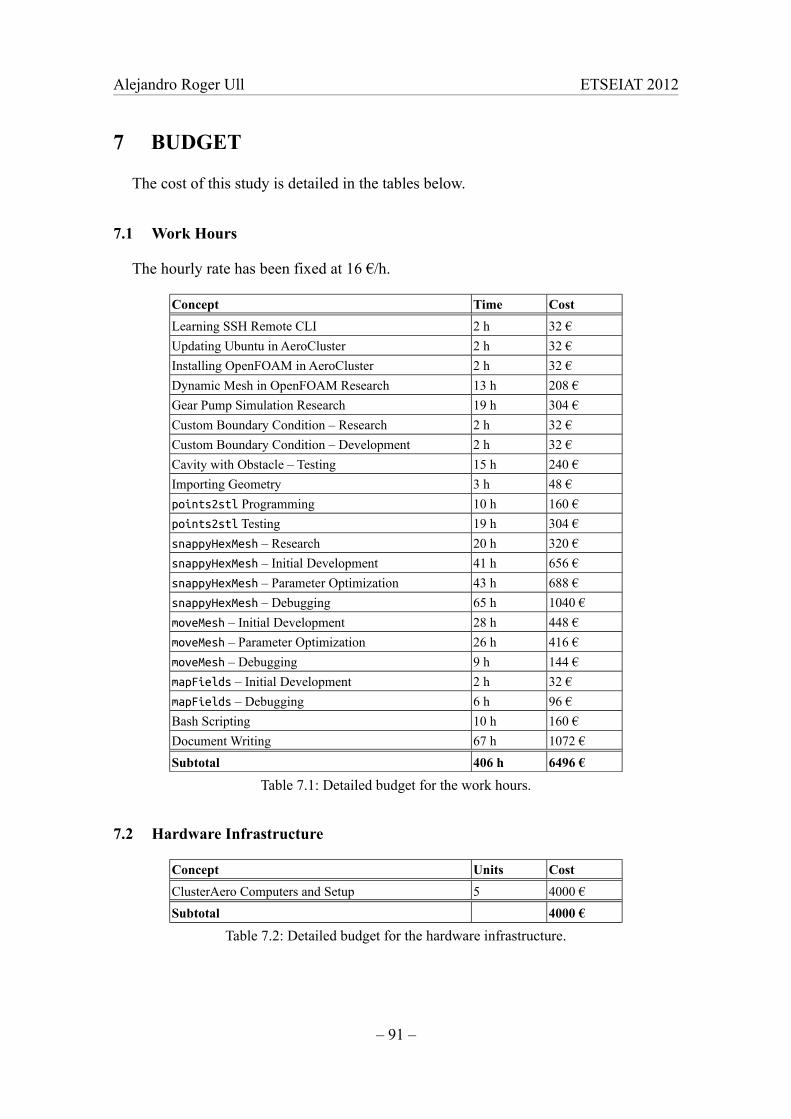
Alejandro Roger Ull ETSEIAT 2012
7 BUDGET
The cost of this study is detailed in the tables below.
7.1 Work Hours
The hourly rate has been fixed at 16 €/h.
Concept Time Cost
Learning SSH Remote CLI 2 h 32 €
Updating Ubuntu in AeroCluster 2 h 32 €
Installing OpenFOAM in AeroCluster 2 h 32 €
Dynamic Mesh in OpenFOAM Research 13 h 208 €
Gear Pump Simulation Research 19 h 304 €
Custom Boundary Condition – Research 2 h 32 €
Custom Boundary Condition – Development 2 h 32 €
Cavity with Obstacle – Testing 15 h 240 €
Importing Geometry 3 h 48 €
points2stl Programming 10 h 160 €
points2stl Testing 19 h 304 €
snappyHexMesh – Research 20 h 320 €
snappyHexMesh – Initial Development 41 h 656 €
snappyHexMesh – Parameter Optimization 43 h 688 €
snappyHexMesh – Debugging 65 h 1040 €
moveMesh – Initial Development 28 h 448 €
moveMesh – Parameter Optimization 26 h 416 €
moveMesh – Debugging 9 h 144 €
mapFields – Initial Development 2 h 32 €
mapFields – Debugging 6 h 96 €
Bash Scripting 10 h 160 €
Document Writing 67 h 1072 €
Subtotal 406 h 6496 €
Table 7.1: Detailed budget for the work hours.
7.2 Hardware Infrastructure
Concept Units Cost
ClusterAero Computers and Setup 5 4000 €
Subtotal 4000 €
Table 7.2: Detailed budget for the hardware infrastructure.
– 91 –
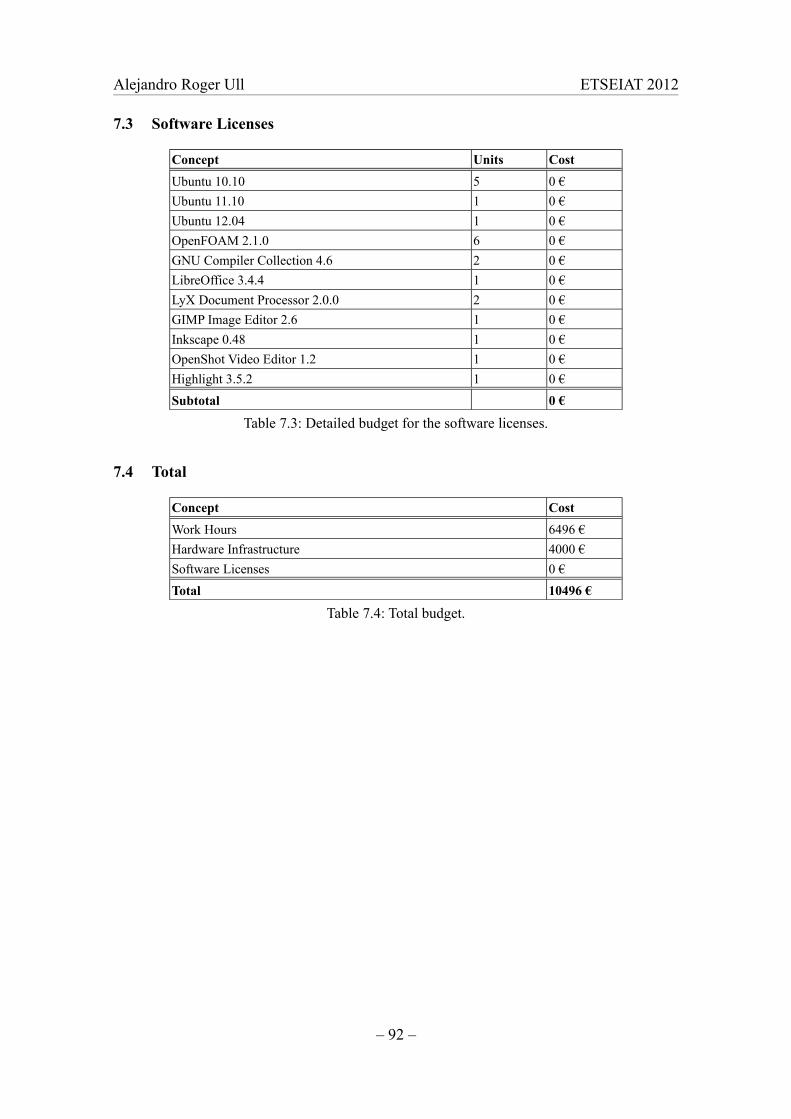
Alejandro Roger Ull ETSEIAT 2012
7.3 Software Licenses
Concept Units Cost
Ubuntu 10.10 5 0 €
Ubuntu 11.10 1 0 €
Ubuntu 12.04 1 0 €
OpenFOAM 2.1.0 6 0 €
GNU Compiler Collection 4.6 2 0 €
LibreOffice 3.4.4 1 0 €
LyX Document Processor 2.0.0 2 0 €
GIMP Image Editor 2.6 1 0 €
Inkscape 0.48 1 0 €
OpenShot Video Editor 1.2 1 0 €
Highlight 3.5.2 1 0 €
Subtotal 0 €
Table 7.3: Detailed budget for the software licenses.
7.4 Total
Concept Cost
Work Hours 6496 €
Hardware Infrastructure 4000 €
Software Licenses 0 €
Total 10496 €
Table 7.4: Total budget.
– 92 –

Alejandro Roger Ull ETSEIAT 2012
8 ENVIRONMENTAL EFFECTS
This study has been entirely computer-based. No residuals were generated during this
work, except from the production of the energy consumed by the computers used, the
computers themselves the day they will be dismantled, and any printed copy or physical
media used to distribute the work.
As such, the only environmental concerns this study arises are to ensure a rational
use of energy, and to properly recycle both the computers and the physical paper or
media should them one day be destroyed.
By following these recommendations the environmental footprint of this study can be
safely considered insignificant, and far below the legal requirements.
– 93 –

Alejandro Roger Ull ETSEIAT 2012
9 REFERENCES
[1] DAVID DEL CAMPO SUD. Analysis of the Suction Chamber of External Gear
Pumps and their Influence on Cavitation and Volumetric Efficiency . A thesis
submitted to the Universitat Politècnica de Catalunya for the degree of Doctor of
Philosophy in the Escola Tècnica Superior d’Enginyeries Industrial i
Aeronàutica de Terrassa, directed by ESTEBAN CODINA MACIÀ and ROBERTO
CASTILLA LÓPEZ. March 2012.
[2] JOSÉ PLÁCIDO PARRA VIOL. Estudio e implementación de nuevas
funcionalidades de deformación de malla en un software de mecánica de fluidos
computacional . Final Project directed by ROBERTO CASTILLA LÓPEZ and DAVID
DEL CAMPO SUD. June 2011.
[3] OpenFOAM User Guide. Online resource. January-June 2012. Available at:
http://www.openfoam.org/docs/user/
[4] OpenFOAM Features Guide. Online resoruce. January-June 2012. Available at:
http://www.openfoam.com/features/
[5] OpenFOAM Advanced Training. Guide for an OpenFOAM version 1.6 course.
October 2009.
[6] HRVOJE JASAK, HENRIK RUSCHE . Dynamic Mesh Handling in OpenFOAM.
Fourth OpenFOAM Workshop, Montreal, Canada, June 2009.
– 95 –