Universita degli Studi di TorinoScuola di Dottorato in Scienza ed Alta Tecnologia

P H D T H E S I S

Study of muon bundles from extensive air showers withALICE detector at the LHC

Katherin Shtejer Diaz

Advisors: Dr. Bruno Alessandro, Prof. Massimo Masera

External reviewer: Prof. Nicola Giglietto

Tesi di Dottorato di Ricerca in Scienza ed Alta TecnologiaIndirizzo di Fisica ed Astrofisica

Academic years: 2013 – 2015Ciclo XXVIII

To my mother Nury

To the memory of my father Guennady

To Emilio

Abstract

The ALICE experiment was mainly designed to study a new phase of mat-

ter, the Quark-Gluon-Plasma (QGP), created in ultra-relativistic heavy-ion

collisions. It is one of the four large experiments at the CERN Large

Hadron Collider (LHC), located in a cavern 52 meters underground with 28

meters of overburden rock. This specific underground location and the ex-

cellent tracking capability of the ALICE Time Projection Chamber (TPC)

have been the cornerstone for a long term program of cosmic ray physics.

Between 2010 and 2013, during pauses in collider operations when

there was no beam circulating in the LHC, ALICE collected approximately

22.6 million events with at least one reconstructed muon in the TPC, being

these muons a component of the extensive air showers (EAS) created by

cosmic ray interactions in the upper atmosphere. The total accumulated

live time was 30.8 days.

In this thesis, the muon multiplicity distribution was measured and com-

pared with predictions from modern Monte Carlo models. A special atten-

tion was dedicated to the study of high multiplicity events, containing more

than 100 reconstructed muons, and corresponding to a muon areal den-

sity ρµ > 5.9±0.4 m−2. Similar events were studied in previous under-

ground experiments, comprised also of accelerator based detectors, such as

ALEPH and DELPHI during the LEP era. While these experiments were

able to reproduce the measured muon multiplicity distribution with Monte

Carlo simulations at low and intermediate multiplicities, their simulations

failed to describe the frequency of the highest multiplicity events.

The results of this thesis demonstrated that multi-muon events collected

iii

iv

in ALICE are due to primary cosmic rays with mixed composition and

energies above 1014 eV, where the average mass of the primary cosmic

rays increases at larger energies. Additionally, the high multiplicity events

observed in ALICE stem from primary cosmic rays with energies above

1016 eV. Our results successfully described the frequency of these events

by assuming a heavy mass composition of primary cosmic rays in this

energy range.

The development of the resulting air showers was simulated using the

latest versions of QGSJET (QGSJET II-03 and QGSJET II-04) to model

hadronic interactions. The predictions of QGSJET II-04, whose parame-

ters were tuned using the early LHC data, reproduced better the measured

rate of the high multiplicity events.

The reliability of the ALICE experiment to collect cosmic ray data, and

to explain them with Monte Carlo simulations using the latest hadronic

interaction models, is confirmed by this study. In particular, for the first

time, the rate of high muon multiplicity events has been reproduced using

conventional models. This result puts stringent limits on alternative, more

exotic, and non-conventional muon production mechanisms.

Contents

1 Introduction 1

2 Cosmic rays 5

2.1 Overview of cosmic rays . . . . . . . . . . . . . . . . . . 5

2.2 Primary cosmic ray spectrum . . . . . . . . . . . . . . . . 7

2.2.1 Spectrum . . . . . . . . . . . . . . . . . . . . . . 8

2.2.2 Composition . . . . . . . . . . . . . . . . . . . . 10

2.2.3 Models . . . . . . . . . . . . . . . . . . . . . . . 13

2.2.4 Origin . . . . . . . . . . . . . . . . . . . . . . . . 17

2.3 Interaction of cosmic radiation with the atmosphere . . . . 18

2.4 Cosmic radiation at surface . . . . . . . . . . . . . . . . . 23

2.5 Cosmic radiation underground . . . . . . . . . . . . . . . 24

2.6 Cosmic radiation measurements . . . . . . . . . . . . . . 26

3 Cosmic ray physics with accelerator detectors 33

3.1 Cosmo-ALEPH experiment . . . . . . . . . . . . . . . . . 33

3.2 DELPHI experiment . . . . . . . . . . . . . . . . . . . . 34

3.3 L3 + C experiment . . . . . . . . . . . . . . . . . . . . . 37

3.4 CMS experiment . . . . . . . . . . . . . . . . . . . . . . 38

4 The ALICE experiment at CERN 41

4.1 Brief picture of the ALICE detector system . . . . . . . . 42

4.2 The detectors used to trigger on atmospheric muons . . . . 43

4.2.1 Inner Tracking System (ITS) . . . . . . . . . . . . 43

v

vi Contents

4.2.2 Time of Flight detector (TOF) . . . . . . . . . . . 44

4.2.3 The ALICE Cosmic Ray Detector (ACORDE) . . 46

4.3 The detector used to track cosmic muons . . . . . . . . . . 46

4.3.1 Time Projection Chamber (TPC) . . . . . . . . . . 46

4.4 Trigger system for cosmic rays in ALICE . . . . . . . . . 48

4.5 The ALICE location and its environment . . . . . . . . . . 51

5 Event reconstruction 55

5.1 Atmospheric muon reconstruction . . . . . . . . . . . . . 55

5.1.1 Tracking algorithm . . . . . . . . . . . . . . . . . 55

5.1.2 Matching algorithm and track selection . . . . . . 56

5.2 Performance of tracking and matching algorithms . . . . . 60

6 Simulation strategy 69

6.1 Event generator and hadronic models . . . . . . . . . . . . 69

6.2 Monte Carlo simulation . . . . . . . . . . . . . . . . . . . 71

6.2.1 CORSIKA initializations . . . . . . . . . . . . . . 73

6.2.2 Simplified Monte Carlo procedure . . . . . . . . . 76

6.2.3 Full Monte Carlo procedure . . . . . . . . . . . . 76

7 Analysis of data and Monte Carlo simulations 77

7.1 Data sample . . . . . . . . . . . . . . . . . . . . . . . . . 77

7.2 Analysis of data and simulations . . . . . . . . . . . . . . 79

7.2.1 Experimental muon multiplicity distribution . . . . 79

7.2.2 High muon multiplicity events . . . . . . . . . . . 80

7.2.3 Simulated muon multiplicity distribution and com-

parison with data . . . . . . . . . . . . . . . . . . 89

7.2.4 Simulated high muon multiplicity events and com-

parison with data . . . . . . . . . . . . . . . . . . 95

Contents vii

8 Discussion of results and Summary 101

1Introduction

ALICE (A Large Ion Collider Experiment) [1] was designed to study Quark-Gluon-Plasma formation in ultra-relativistic heavy-ion collisions at the CERNLarge Hadron Collider. The QGP is a high temperature and high density phaseof strongly interacting matter, predicted by quantum chromodynamics (QCD)and whose existence is now firmly established experimentally [2]. Althoughits main purpose is to explore the properties of the QGP, the ALICE spectrom-eter has been also used to perform studies of relevance in cosmic-ray physics.

The ALICE location at 52 meters underground with 28 meters of over-burden rock, results very convenient to measure muons produced by cosmicray interactions in the atmosphere. During pauses in collider operations whenthere was no beam circulating in the LHC, ALICE undertook a programme ofcosmic ray data taking between 2010 and 2013, taking advantage of the largesize and excellent tracking capability of its Time Projection Chamber [3]. Thetotal accumulated run time amounted to 30.8 days, resulting in approximately22.6 million events with at least one reconstructed muon in the ALICE TPC.

Cosmic ray muons are created in Extensive Air Showers (EAS) followingthe interaction of cosmic ray primaries (protons and heavier nuclei) with nu-clei of the upper atmosphere. Primary cosmic rays span a broad energy range,from approximately 109 eV to about 1021 eV. At energies lower than 1015

eV, the high flux of cosmic rays can be measured directly at different altitudesof the atmosphere. At energies in the range 1014 < E < 1021 eV, where di-rect measurements are no longer possible, larger detector areas are needed toachieve reasonable statistics. These indirect measurements detect secondaryparticles produced in EAS. In this thesis we will cover indirect measurementssince ALICE detects the muonic component of EAS at energies around 1015

eV.Several experiments have been devoted to study the EAS development

through the detection of its components. Many of them such as large-areadetector arrays at ground level [4–6] and underground facilities [7–9] perform

1

2 Introduction

indirect measurements of cosmic rays at energies in the knee region (E ∼ 1015

eV), while others study cosmic rays at energies well above the knee, coveringthe ultra-energetic cosmic rays [10–13].

The study of the mass composition and the energy spectrum of primarycosmic rays around and above the knee is crucial to explore the sources ofcosmic rays arriving at the Earth. Although the composition of primary cosmicrays around this energy is a mixture of many species of nuclei in a ratio that isnot well known, measurements indicate that a notable change of the chemicalcomposition takes place at this energy, favouring heavier components as theenergy of primary particles increases.

In the spite of their small size, compared with the standard cosmic-ray ex-periments, the use of underground accelerator-based detectors to study thehigh-energy muonic component of the EAS becomes a promising opportunityto understand the early shower development, since energetic muons are pro-duced in the very first interactions, thus carrying valuable information aboutthe primary cosmic particles. The use of high-energy physics detectors forcosmic ray physics was pioneered by ALEPH[14], DELPHI [15] and L3 [16]during the Large Electron-Positron (LEP) collider [17] era at CERN.

The muon multiplicity distribution (MMD) was measured at LEP with theALEPH detector [14]. This study concluded that the bulk of data can be suc-cessfully described using standard hadronic production mechanisms, but thatthe highest multiplicity events containing around 75-150 muons, occur with afrequency which is almost an order of magnitude above the expectation, evenwhen assuming that the primary cosmic rays are purely composed of iron nu-clei. A similar study was carried out by DELPHI detector, which also foundthat Monte Carlo simulations were unable to account for the abundance ofhigh muon multiplicity events [15]. An extension of these earlier studies isnow possible at the LHC, where the ALICE capabilities are exploited withthis purpose.

I participated in the cosmic-ray data taking of 2012 and 2013 and workedin the analysis of the atmospheric muon events detected in the ALICE ex-periment in the whole period 2010-2013. My research activities were mainlyfocused to the study of the measured muon multiplicity distribution and itscomparison with Monte Carlo simulations. I have also investigated in detailsthe high muon multiplicity (HMM) events found with data, that is, events witha number of reconstructed muons in the TPC larger than 100 (Nµ > 100).

3

The description of the shower in the Monte Carlo simulations is based upontwo of the latest versions of QGSJET [18, 19], a hadronic interaction modelcommonly used in EAS simulations.

In the following chapter [2] I summarize the properties of cosmic rays andpresent the characteristics of the shower development at different stages, aswell as a brief description of its measurement methods. Results of cosmic-raystudies performed by previous experiments based upon high-energy physicsdetectors, are presented in chapter 3. In chapter 4, a general description ofthe ALICE experiment is presented, specifically of the detector subsystemsused to perform cosmic ray physics. Chapter 5 introduces the methods im-plemented to reconstruct events and the track selection criteria. In addition,the Monte Carlo simulations to reproduce the experimental results required acareful selection of the event generator and models to describe the extensiveair showers, as well as the strategy to assure the accuracy and efficiency ofthe simulations. This is described in chapter 6. In chapter 7, the characteris-tics of the data sample analysed in this thesis are presented. The analysis ofthe MMD from data and simulations is discussed, as well as the measurementsand interpretation of the frequency of HMM events. The systematic and statis-tical uncertainties are described during the analysis evolution. The discussionof the final results from the comparison between data and model predictionsare discussed in chapter 8, where also the final summary is given.

2Cosmic rays

2.1 Overview of cosmic rays

Cosmic rays became one of the most fascinating research subjects in modernphysics and astronomy since its revolutionary discovery by Victor Franz Hessin 1912. Today, more than one hundred years later the question about theorigin of the cosmic radiation still remains unanswered. The main sources ofcosmic rays are considered to be the stars, supernova remnants, pulsars, activegalactic nuclei, black holes and gamma ray bursts.

Cosmic ray physics has played an important role in the formation of ourcurrent understanding of the universe evolution, representing a vast and widefield of research. Hess’s discovery contributed to develop the modern physicsand astronomy with new fields of research such as particle physics, modernastrophysics and cosmology. The importance of cosmic rays for differentbranches of sciences started to be better understood in 1932 with the discov-ery of the positron, and since then many new particles were first reported tooccur in cosmic rays. Such is the case of elementary particles like mesonsand hyperons, new types of nuclear reactions at high energies, formation ofnuclear-meson and electromagnetic cascades in the atmosphere. All of thiswas discovered during the investigation of cosmic rays, which became a greattool for exploring the fundamental building blocks of matter.

Another important branch of physics that has rapidly evolved together withspace exploration, concerns the cosmic-ray energy spectrum, as well as theorigin, acceleration and propagation of the cosmic radiation, representing areal challenge for astrophysics, astronomy and cosmology. At present otherrelevant fields have rapidly evolved, such as high-energy gamma ray and neu-trino astronomy. Moreover, geophysical researches of the interior of the Earthare starting under high-energy neutrino astronomy which is likely a spin-offneutrino tomography of the Earth. Finally, of considerable interest are thebiological and medical aspects of the cosmic radiation, because of its ioniz-

5

6 Cosmic rays

ing character and the fact of being the unavoidable radiation to which we areexposed.

Since the investigations of air conductivity, started by Coulomb in 1785,physics faced the problem of explaining the leakage of electrical charge fromvery isolated bodies. At the beginning of 20th century, in connection withthe discovery of natural radioactivity, many ingenious experiments were per-formed in order to solve the puzzle of the nature of such radiation responsiblefor the electric charge loss observed in isolated electroscopes. The questionof whether it was of terrestrial or extraterrestrial origin was crucial. In thespite of the terrestrial origin as the simplest hypothesis considered in that time,Wilson made a suggestion without precedents that such extremely penetratingradiation could have extraterrestrial origin. However this idea was not sup-ported by his experiments. During 2011 the Italian physicist Domenico Pacinidemonstrated that a non-negligible part of the mentioned radiations was notcoming from the Earth’s crust [20]. This was confirmed by measuring thevariations of an electroscope’s discharge rate as a function of the underwaterdepth. Paccini’s conclusions about the presence of a non terrestrial radia-tion at sea level were supported by the results from other scientists pointingto the dependence of the radioactivity on the altitude. By following differ-ent and complementary methods, these radiations were evidenced by VictorF. Hess during its historical hydrogen-filled balloon flights in 1912 [21]. Theexpectation was that the flux would decrease with the altitude, precisely theopposite of what Hess found. He determined that up to approximately oneKm the ionization was unchanged, however with the increasing altitude upto approximately 5.3 Km the ionization rates escalated several times. Hessdrew the conclusion that certain unknown radiation source of ionization ofextraterrestrial origin exists, meaning that particles arrived to the Earth fromspace. This radiation was first named “cosmic rays” by Millikan in 1926 [22].In absorption measurements of the radiation at different depths and altitudes,Cameron and Millikan concluded that the radiation consisted of high-energygamma rays. Nevertheless, Bothe and Kolhorster demonstrated that cosmicrays consist mainly of charged particles, by using for the first time a coin-cidence technique with Geiger Muller counters [23]. The highly penetratingpower of cosmic rays was proved by making them traverse a gold absorberplaced between two Geiger Muller counters. In 1929 Skobelzyn registeredthe deviation suffered by cosmic ray in a bubble detector with magnetic field.

2.2 Primary cosmic ray spectrum 7

He also suggested that these particles were produced in showers [24] whilein 1937 Pierre Auger concluded that the extensive particle showers are gener-ated by high-energy primary cosmic-ray particles that interact with air nucleihigh in the atmosphere, initiating a cascade of secondary interactions that fi-nally yield a shower of electrons, photons and muons that reach ground level[25]. Later in 1941 was established that cosmic rays are composed mostly byenergetic protons constituting ∼ 89%, about 10% He nuclei, ∼ 1% heaviernuclei like C, N, O and Fe, while less than 1% energetic electrons and gammarays [26].

Today, after one hundred years since the discovery of cosmic radiation, itsorigin remains unknown. Various objects in our Galaxy have been proposedas particle injectors and different acceleration mechanisms are known to havethe ability to accelerate or possibly reaccelerate cosmic rays to energies ofabout 1014-1018 eV, although propagation mechanisms are subject of intensedebate. Actually, it is a mystery where and how the most energetic particleswith more than 1018 eV acquire their energies, though various exotic modelsand processes have been proposed.

2.2 Primary cosmic ray spectrum

The term cosmic radiation is referred to the flux of high energy particles, thatenter the Earth’s atmosphere from the outer space. It includes all stable parti-cles and nuclei with lifetimes of the order of 106 years or longer. Technically,“primary” cosmic rays are those particles accelerated at astrophysical sourceswhereas “secondaries” are those particles produced in interactions of the pri-maries with interstellar gas. Most of cosmic radiation comes from outside theSolar System, except from particles associated with solar flares. The SolarSystem is permanently exposed to a flux of these primary particles, with aspectrum extending over many orders of magnitude from about 109 eV to atleast 1020 eV, while the secondaries generated in these first encounters havestill enough energy to produce further particles. Cosmic rays are exposed todifferent magnetic fields in their trajectory from the origin to the Earth, i.e.,magnetic field of Earth, Solar System and Galaxy. Consequently the cosmicrays cannot point to the source since they are composed by charged particlesbeing constantly deflected by the magnetic fields.

In the following we call “primary” cosmic rays to all high energy particles

8 Cosmic rays

arriving to the Earth atmosphere from the outer space, with either galactic orextragalactic origin. The interaction of primary cosmic rays with the nuclei ofthe air constituent elements in the upper Earth atmosphere, gives rise to the so-called Extensive Air Showers (EAS) which evolve until ionization processesdominate and the cascade dies out.

2.2.1 Spectrum

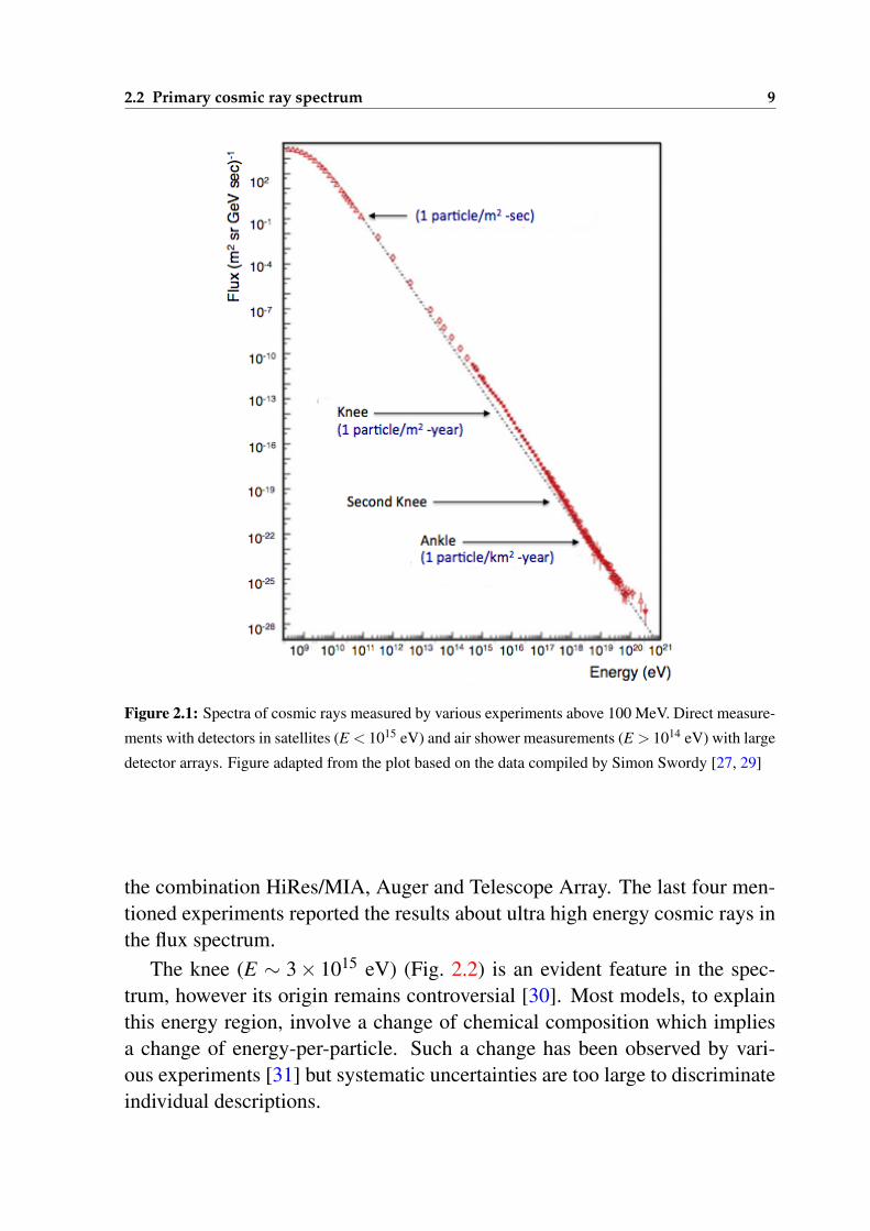
The differential cosmic ray spectrum, i.e. the number of primary atomic nu-clei arriving at the Earth per unit time, area, solid angle and kinetic energy,follows a relatively smooth power law dN/dE ∝ Eγ over a wide energy range(Fig. 2.1) [27]. At low energies this flux is modulated by the solar cyclethrough the magnetic field of the Sun1, which shields the Solar System fromcharged particles below 109 eV. In the range of several GeV (∼ 109 eV) toabout Ek = 3×1015 eV, the primary cosmic-ray energy spectrum is well de-scribed by a power law with spectral index γ ≈-2.7. At higher energies thespectrum index changes rapidly to γ ≈-3.1 creating a ‘transition’ region atE = Ek called the “knee”. The further steepening indicates a second “knee”which is observed at Ekk = 4×1017 eV. At about Ea = 3×1018 eV the spec-trum hardens again giving rise to a feature called the “ankle”. Beyond theankle the spectrum is more difficult to quantify.

The mentioned features (knees and ankle) of the primary cosmic ray spec-trum are better evidenced when the ordinate is multiplied by some power of theparticle energy as shown in figure 2.2. In this figure the total flux is the resultof data obtained by several experiments whereas the energy is compared withthe equivalent centre-of-mass energy of proton induced collisions at variousaccelerators. As shown in figure 2.2, the flux at energies below∼ 1014 eV wasobtained from results of direct measurements like ATIC, PROTON and RUN-JOB. Data from direct measurements together with results from the ground ar-ray Tibet AS-gamma experiment aimed to measure the EAS, helped to shapethe flux at 1014 < E < 1015 eV. The energies around the knee (E ∼ 3× 1015

eV) and beyond, just up to E ∼ 1020 eV, were covered by several results fromEAS measurements compared with hadronic interaction models. This is thecase of KASCADE, KASCADE-Grande, Tibet AS-gamma, IceTop, HiRes,

1At energies E < 109 eV the screening effect of the solar wind prevents galactic cosmic rays from penetratingthe heliosphere [28], so that the low energy particle flux decreases during periods of high solar activity andreaches its maximum during phases of low solar activity. This phenomenon is known as solar modulation.

2.2 Primary cosmic ray spectrum 9

Figure 2.1: Spectra of cosmic rays measured by various experiments above 100 MeV. Direct measure-

ments with detectors in satellites (E < 1015 eV) and air shower measurements (E > 1014 eV) with large

detector arrays. Figure adapted from the plot based on the data compiled by Simon Swordy [27, 29]

the combination HiRes/MIA, Auger and Telescope Array. The last four men-tioned experiments reported the results about ultra high energy cosmic rays inthe flux spectrum.

The knee (E ∼ 3× 1015 eV) (Fig. 2.2) is an evident feature in the spec-trum, however its origin remains controversial [30]. Most models, to explainthis energy region, involve a change of chemical composition which impliesa change of energy-per-particle. Such a change has been observed by vari-ous experiments [31] but systematic uncertainties are too large to discriminateindividual descriptions.

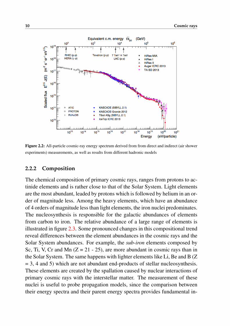
10 Cosmic rays

Figure 2.2: All-particle cosmic-ray energy spectrum derived from from direct and indirect (air shower

experiments) measurements, as well as results from different hadronic models

2.2.2 Composition

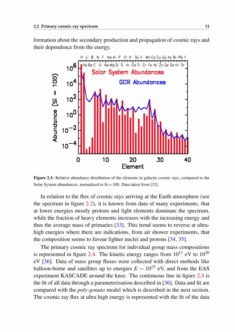
The chemical composition of primary cosmic rays, ranges from protons to ac-tinide elements and is rather close to that of the Solar System. Light elementsare the most abundant, leaded by protons which is followed by helium in an or-der of magnitude less. Among the heavy elements, which have an abundanceof 4 orders of magnitude less than light elements, the iron nuclei predominates.The nucleosynthesis is responsible for the galactic abundances of elementsfrom carbon to iron. The relative abundance of a large range of elements isillustrated in figure 2.3. Some pronounced changes in this compositional trendreveal differences between the element abundances in the cosmic rays and theSolar System abundances. For example, the sub-iron elements composed bySc, Ti, V, Cr and Mn (Z = 21 - 25), are more abundant in cosmic rays than inthe Solar System. The same happens with lighter elements like Li, Be and B (Z= 3, 4 and 5) which are not abundant end-products of stellar nucleosynthesis.These elements are created by the spallation caused by nuclear interactions ofprimary cosmic rays with the interstellar matter. The measurement of thesenuclei is useful to probe propagation models, since the comparison betweentheir energy spectra and their parent energy spectra provides fundamental in-

2.2 Primary cosmic ray spectrum 11

formation about the secondary production and propagation of cosmic rays andtheir dependence from the energy.

Figure 2.3: Relative abundance distribution of the elements in galactic cosmic rays, compared to the

Solar System abundances, normalised to Si = 100. Data taken from [32].

In relation to the flux of cosmic rays arriving at the Earth atmosphere (seethe spectrum in figure 2.2), it is known from data of many experiments, thatat lower energies mostly protons and light elements dominate the spectrum,while the fraction of heavy elements increases with the increasing energy andthus the average mass of primaries [33]. This trend seems to reverse at ultra-high energies where there are indications, from air shower experiments, thatthe composition seems to favour lighter nuclei and protons [34, 35].

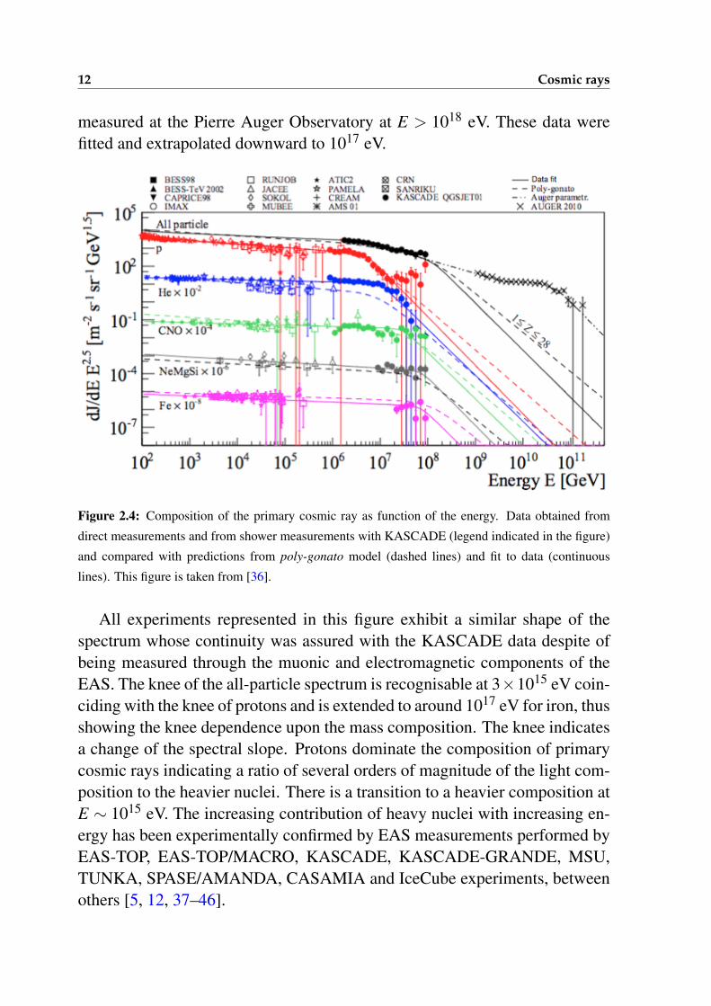
The primary cosmic ray spectrum for individual group mass compositionsis represented in figure 2.4. The kinetic energy ranges from 1011 eV to 1020

eV [36]. Data of mass group fluxes were collected with direct methods likeballoon-borne and satellites up to energies E ∼ 1015 eV, and from the EASexperiment KASCADE around the knee. The continuous line in figure 2.4 isthe fit of all data through a parameterisation described in [36]. Data and fit arecompared with the poly-gonato model which is described in the next section.The cosmic ray flux at ultra high energy is represented with the fit of the data

12 Cosmic rays

measured at the Pierre Auger Observatory at E > 1018 eV. These data werefitted and extrapolated downward to 1017 eV.

Figure 2.4: Composition of the primary cosmic ray as function of the energy. Data obtained from

direct measurements and from shower measurements with KASCADE (legend indicated in the figure)

and compared with predictions from poly-gonato model (dashed lines) and fit to data (continuous

lines). This figure is taken from [36].

All experiments represented in this figure exhibit a similar shape of thespectrum whose continuity was assured with the KASCADE data despite ofbeing measured through the muonic and electromagnetic components of theEAS. The knee of the all-particle spectrum is recognisable at 3×1015 eV coin-ciding with the knee of protons and is extended to around 1017 eV for iron, thusshowing the knee dependence upon the mass composition. The knee indicatesa change of the spectral slope. Protons dominate the composition of primarycosmic rays indicating a ratio of several orders of magnitude of the light com-position to the heavier nuclei. There is a transition to a heavier composition atE ∼ 1015 eV. The increasing contribution of heavy nuclei with increasing en-ergy has been experimentally confirmed by EAS measurements performed byEAS-TOP, EAS-TOP/MACRO, KASCADE, KASCADE-GRANDE, MSU,TUNKA, SPASE/AMANDA, CASAMIA and IceCube experiments, betweenothers [5, 12, 37–46].

2.2 Primary cosmic ray spectrum 13

2.2.3 Models

The understanding of the origin of the knee in the all-particle spectrum of pri-mary cosmic rays has been a long-standing problem in astrophysics, since itis probably related to the source composition and the mechanisms of acceler-ation and propagation in the Galaxy (see [47] and references therein).

In the following, there is a general and summarised picture about some the-oretical models devoted to explain the knee issue, as well as the phenomeno-logical model called poly-gonato.

Theoretical models

Different models offer possible explanations to the change of the slope in theenergy spectrum of primary cosmic rays. They interpret the knee in differentways:

• The knee as an indication of a limit where the acceleration mechanismsstart to be less efficient.

• The knee as a consequence of the cosmic ray escaping from the galaxy.

• The knee connected with physics processes during the EAS evolution.

The first two items are respectively related to the acceleration and diffu-sive propagation of cosmic rays produced in supernova explosions throughthe Galaxy. Several approaches can be found in the literature, where differentacceleration mechanisms have been addressed as responsible for the existenceof the knee. The common idea is that a substantial amount of the energy re-leased in the supernova explosion is transferred to the ionized particles in formof kinetic energy. According to that, the reachable energy in the accelerationprocess is proportional to the charge Z of the nuclei, albeit it also depends onthe strength of the magnetic field and the characteristic time of acceleration.Some models considering the acceleration of supernova remnants as responsi-ble of the knee, suggest that cosmic rays may reach energies of Z×1014 eV,which has been also stablished by experimental observations and is consis-tently described by the theory of diffusive shock acceleration. In other modelsthe injection efficiency is expected to be a function of the mass to charge ratio,such that the heavy elements are accelerated more efficiently and enrich thecosmic rays making the spectrum harder [48].

14 Cosmic rays

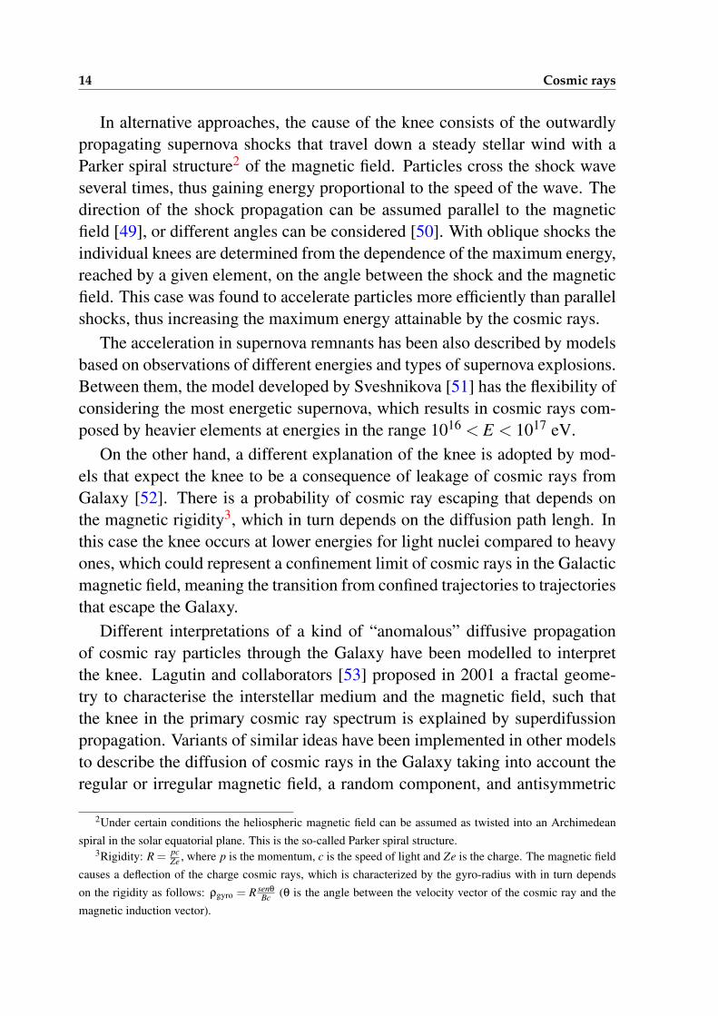
In alternative approaches, the cause of the knee consists of the outwardlypropagating supernova shocks that travel down a steady stellar wind with aParker spiral structure2 of the magnetic field. Particles cross the shock waveseveral times, thus gaining energy proportional to the speed of the wave. Thedirection of the shock propagation can be assumed parallel to the magneticfield [49], or different angles can be considered [50]. With oblique shocks theindividual knees are determined from the dependence of the maximum energy,reached by a given element, on the angle between the shock and the magneticfield. This case was found to accelerate particles more efficiently than parallelshocks, thus increasing the maximum energy attainable by the cosmic rays.

The acceleration in supernova remnants has been also described by modelsbased on observations of different energies and types of supernova explosions.Between them, the model developed by Sveshnikova [51] has the flexibility ofconsidering the most energetic supernova, which results in cosmic rays com-posed by heavier elements at energies in the range 1016 < E < 1017 eV.

On the other hand, a different explanation of the knee is adopted by mod-els that expect the knee to be a consequence of leakage of cosmic rays fromGalaxy [52]. There is a probability of cosmic ray escaping that depends onthe magnetic rigidity3, which in turn depends on the diffusion path lengh. Inthis case the knee occurs at lower energies for light nuclei compared to heavyones, which could represent a confinement limit of cosmic rays in the Galacticmagnetic field, meaning the transition from confined trajectories to trajectoriesthat escape the Galaxy.

Different interpretations of a kind of “anomalous” diffusive propagationof cosmic ray particles through the Galaxy have been modelled to interpretthe knee. Lagutin and collaborators [53] proposed in 2001 a fractal geome-try to characterise the interstellar medium and the magnetic field, such thatthe knee in the primary cosmic ray spectrum is explained by superdifussionpropagation. Variants of similar ideas have been implemented in other modelsto describe the diffusion of cosmic rays in the Galaxy taking into account theregular or irregular magnetic field, a random component, and antisymmetric

2Under certain conditions the heliospheric magnetic field can be assumed as twisted into an Archimedeanspiral in the solar equatorial plane. This is the so-called Parker spiral structure.

3Rigidity: R = pcZe , where p is the momentum, c is the speed of light and Ze is the charge. The magnetic field

causes a deflection of the charge cosmic rays, which is characterized by the gyro-radius with in turn dependson the rigidity as follows: ρgyro = R senθ

Bc (θ is the angle between the velocity vector of the cosmic ray and themagnetic induction vector).

2.2 Primary cosmic ray spectrum 15

or Hall diffusion [54–56].The essential common feature of the processes of particle reaccelerating

and diffusion is the magnetic rigidity dependence. From the astrophysicalpoint of view a rigidity dependent cutoff (EZ ∝ Z) is most likely the descrip-tion, but since the origin of the knee is still under discussion other explanationsfor the change of the spectra slope are possible.

Following a different point of view, there are models that do not “see” thesource of the knee in the interstellar medium but in the Earth atmosphere (seethird item at the beginning of this section). They suggest that a new type ofinteraction transfers energy to an unknown or not yet observed componentof air showers. The threshold of these new interactions is proposed to be inthe knee region. Particles undetected by experimental apparatus, like possiblelightest supersymmetric particles and gravitons produced in a sort of “new”EAS interactions, have been suggested by Kazanas [57, 58] as responsible ofthe steepening at the knee. These approaches have in common that the kneefor individual elements scales with their mass number A and not with theirnuclear change Z.

Most of the models produce similar all-particle spectra although their ba-sis suggest different theoretical origins of the knee. In general the maximumenergy attainable by a nucleus of charge Z differs on the model and types ofsupernovae considered. The spectra of individual group compositions do notnecessarily agree, however most of the models suggest that the knee wouldresult from the convolution of various cutoffs while the spectra compositionbecome heavier, establishing different kind of relationships with particular as-pects of acceleration and propagation mechanisms. Maybe the explanationabout the cause of the knee in the cosmic ray spectrum comes from the inte-gration of various model basis, e.g. by including injection, acceleration andpropagation. The most feasible explanation for the knee seems to be a combi-nation of the maximum energy reached during acceleration and leakage fromthe Galaxy during propagation, however at present no model can be excluded.

Poly-gonato model

One of the more accepted models, that explains the slope changes in the kneeregion is the poly-gonato4 phenomenological model [47]. The model assumes

4 From Greek: “many knees”.

16 Cosmic rays

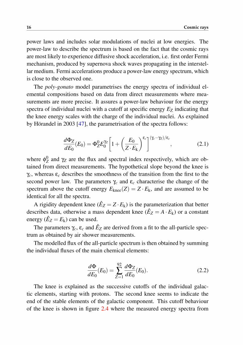
power laws and includes solar modulations of nuclei at low energies. Thepower-law to describe the spectrum is based on the fact that the cosmic raysare most likely to experience diffusive shock acceleration, i.e. first order Fermimechanism, produced by supernova shock waves propagating in the interstel-lar medium. Fermi accelerations produce a power-law energy spectrum, whichis close to the observed one.

The poly-gonato model parametrises the energy spectra of individual el-emental compositions based on data from direct measurements where mea-surements are more precise. It assures a power-law behaviour for the energyspectra of individual nuclei with a cutoff at specific energy EZ indicating thatthe knee energy scales with the charge of the individual nuclei. As explainedby Horandel in 2003 [47], the parametrisation of the spectra follows:

dΦZ

dE0(E0) = Φ

0ZEγZ

0

[1+(

E0

Z ·Ek

)εc](γc−γZ)/εc

, (2.1)

where φ0Z and γZ are the flux and spectral index respectively, which are ob-

tained from direct measurements. The hypothetical slope beyond the knee isγc, whereas εc describes the smoothness of the transition from the first to thesecond power law. The parameters γc and εc characterise the change of thespectrum above the cutoff energy Eknee(Z) = Z ·Ek, and are assumed to beidentical for all the spectra.

A rigidity dependent knee (EZ = Z ·Ek) is the parameterization that betterdescribes data, otherwise a mass dependent knee (EZ = A ·Ek) or a constantenergy (EZ = Ek) can be used.

The parameters γc, εc and EZ are derived from a fit to the all-particle spec-trum as obtained by air shower measurements.

The modelled flux of the all-particle spectrum is then obtained by summingthe individual fluxes of the main chemical elements:

dΦ

dE0(E0) =

92

∑Z=1

dΦZ

dE0(E0). (2.2)

The knee is explained as the successive cutoffs of the individual galac-tic elements, starting with protons. The second knee seems to indicate theend of the stable elements of the galactic component. This cutoff behaviourof the knee is shown in figure 2.4 where the measured energy spectra from

2.2 Primary cosmic ray spectrum 17

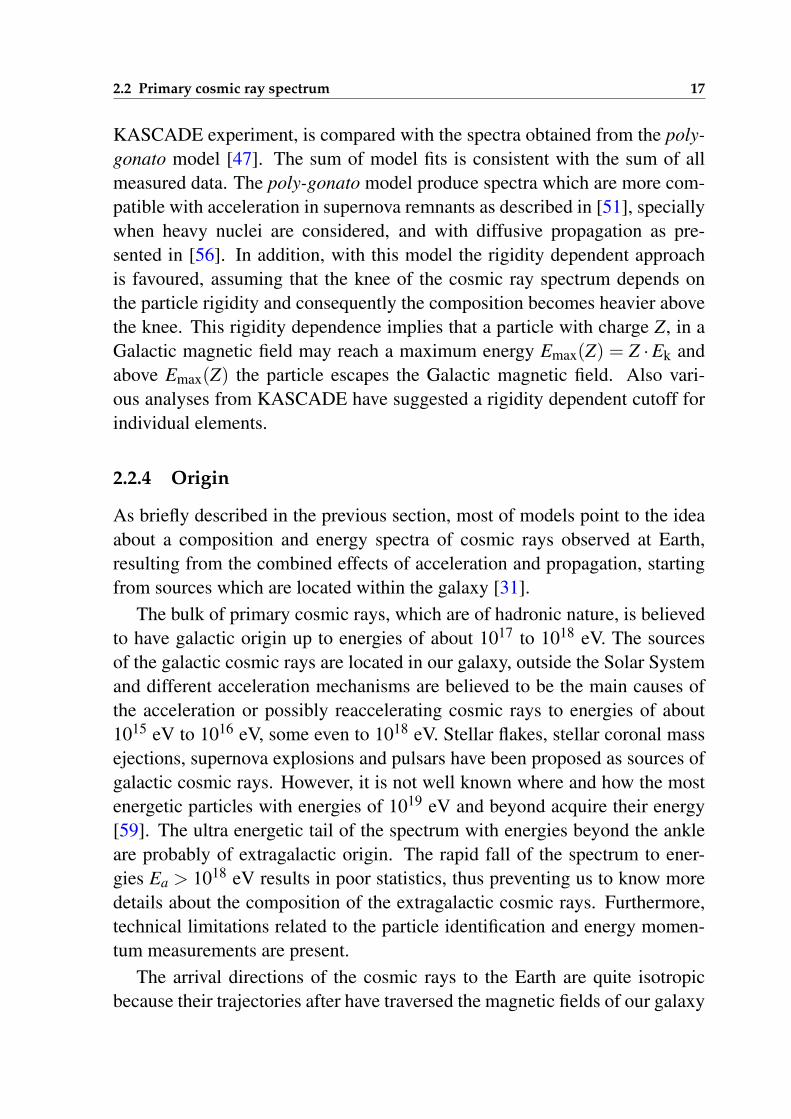
KASCADE experiment, is compared with the spectra obtained from the poly-gonato model [47]. The sum of model fits is consistent with the sum of allmeasured data. The poly-gonato model produce spectra which are more com-patible with acceleration in supernova remnants as described in [51], speciallywhen heavy nuclei are considered, and with diffusive propagation as pre-sented in [56]. In addition, with this model the rigidity dependent approachis favoured, assuming that the knee of the cosmic ray spectrum depends onthe particle rigidity and consequently the composition becomes heavier abovethe knee. This rigidity dependence implies that a particle with charge Z, in aGalactic magnetic field may reach a maximum energy Emax(Z) = Z ·Ek andabove Emax(Z) the particle escapes the Galactic magnetic field. Also vari-ous analyses from KASCADE have suggested a rigidity dependent cutoff forindividual elements.

2.2.4 Origin

As briefly described in the previous section, most of models point to the ideaabout a composition and energy spectra of cosmic rays observed at Earth,resulting from the combined effects of acceleration and propagation, startingfrom sources which are located within the galaxy [31].

The bulk of primary cosmic rays, which are of hadronic nature, is believedto have galactic origin up to energies of about 1017 to 1018 eV. The sourcesof the galactic cosmic rays are located in our galaxy, outside the Solar Systemand different acceleration mechanisms are believed to be the main causes ofthe acceleration or possibly reaccelerating cosmic rays to energies of about1015 eV to 1016 eV, some even to 1018 eV. Stellar flakes, stellar coronal massejections, supernova explosions and pulsars have been proposed as sources ofgalactic cosmic rays. However, it is not well known where and how the mostenergetic particles with energies of 1019 eV and beyond acquire their energy[59]. The ultra energetic tail of the spectrum with energies beyond the ankleare probably of extragalactic origin. The rapid fall of the spectrum to ener-gies Ea > 1018 eV results in poor statistics, thus preventing us to know moredetails about the composition of the extragalactic cosmic rays. Furthermore,technical limitations related to the particle identification and energy momen-tum measurements are present.

The arrival directions of the cosmic rays to the Earth are quite isotropicbecause their trajectories after have traversed the magnetic fields of our galaxy

18 Cosmic rays

are randomly bent. However, at a certain energy threshold of the order of1018 eV the cosmic rays escape the galaxy following trajectories which arealmost straight lines. Their sources must be very distant in order to allow fordirectional randomisation by magnetic fields in space. This reinforces the ideaabout their extragalactic origin, in whose case it is a puzzle how these particlescan reach our part of the universe across large distances without being subjectto the Greisen-Zatsepin-Kuzmin (GZK) cutoff, expected to occur around E =

3− 5× 1019 eV for protons [60, 61]. This cutoff is due to interactions of thecosmic rays with the cosmic microwave background (CMBR), predicted since1948 [62] and discovered by Penzias and Wilson in 1965 [63], that degrade theenergy of particles via photo-pion production and fragment nuclei until theirenergies fall below the GZK-limit.

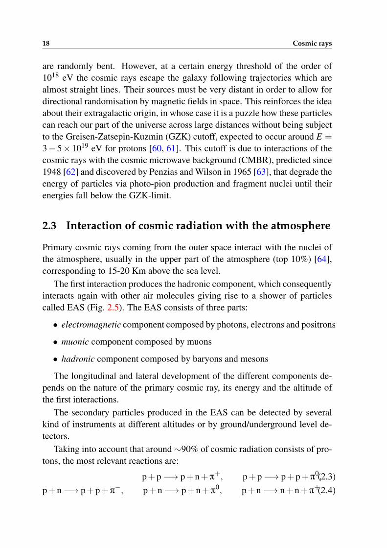
2.3 Interaction of cosmic radiation with the atmosphere

Primary cosmic rays coming from the outer space interact with the nuclei ofthe atmosphere, usually in the upper part of the atmosphere (top 10%) [64],corresponding to 15-20 Km above the sea level.

The first interaction produces the hadronic component, which consequentlyinteracts again with other air molecules giving rise to a shower of particlescalled EAS (Fig. 2.5). The EAS consists of three parts:

• electromagnetic component composed by photons, electrons and positrons

• muonic component composed by muons

• hadronic component composed by baryons and mesons

The longitudinal and lateral development of the different components de-pends on the nature of the primary cosmic ray, its energy and the altitude ofthe first interactions.

The secondary particles produced in the EAS can be detected by severalkind of instruments at different altitudes or by ground/underground level de-tectors.

Taking into account that around ∼90% of cosmic radiation consists of pro-tons, the most relevant reactions are:

p+p−→ p+n+π+, p+p−→ p+p+π

0,(2.3)p+n−→ p+p+π

−, p+n−→ p+n+π0, p+n−→ n+n+π

+.(2.4)

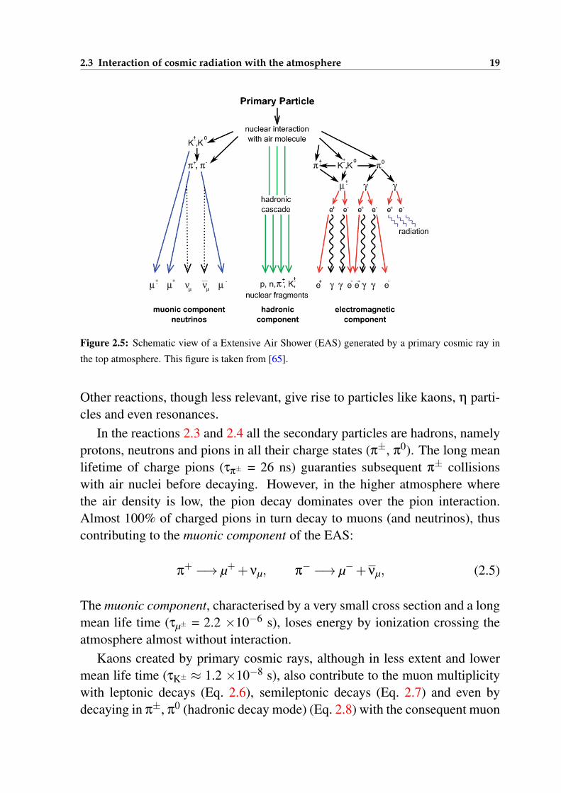
2.3 Interaction of cosmic radiation with the atmosphere 19

Figure 2.5: Schematic view of a Extensive Air Shower (EAS) generated by a primary cosmic ray in

the top atmosphere. This figure is taken from [65].

Other reactions, though less relevant, give rise to particles like kaons, η parti-cles and even resonances.

In the reactions 2.3 and 2.4 all the secondary particles are hadrons, namelyprotons, neutrons and pions in all their charge states (π±, π0). The long meanlifetime of charge pions (τπ± = 26 ns) guaranties subsequent π± collisionswith air nuclei before decaying. However, in the higher atmosphere wherethe air density is low, the pion decay dominates over the pion interaction.Almost 100% of charged pions in turn decay to muons (and neutrinos), thuscontributing to the muonic component of the EAS:

π+ −→ µ++νµ, π

− −→ µ−+νµ, (2.5)

The muonic component, characterised by a very small cross section and a longmean life time (τµ± = 2.2 ×10−6 s), loses energy by ionization crossing theatmosphere almost without interaction.

Kaons created by primary cosmic rays, although in less extent and lowermean life time (τK± ≈ 1.2 ×10−8 s), also contribute to the muon multiplicitywith leptonic decays (Eq. 2.6), semileptonic decays (Eq. 2.7) and even bydecaying in π±, π0 (hadronic decay mode) (Eq. 2.8) with the consequent muon

20 Cosmic rays

production from π±.

K+ −→ µ++νµ, K− −→ µ−+νµ, (2.6)K+ −→ π

0 +µ++νµ, K− −→ π0 +µ−+νµ, (2.7)

K+ −→ π++π

0, K− −→ π−+π

0, (2.8)

The major contribution to the electromagnetic component comes from neutralpions by decaying in two photons in a very short mean life time (τπ0 = 10−16

s):

π0 −→ γ+ γ, (2.9)

although the following muon decay channels contribute to the positron andelectron production as well:

µ+ −→ e++νe +νµ and µ− −→ e−+νe +νµ. (2.10)

The two photons created from neutral pions (Eq. 2.9), give rise to electron-positron pairs, thus emitting bremsstrahlung photons when the mean electronenergies are above a critical energy Ee = 84 MeV. Below Ee, ionization pro-cesses dominate over radiative losses.

The vertical fluxes of the major cosmic ray components in the atmosphereare shown in figure 2.6. Except for protons near the top of the atmosphere,all particles are produced in interactions of the primary cosmic rays in the air(Eqs. 2.5–2.9).

The hadronic component of the EAS constitutes the core of the cascade.Since high hadron energies assure a longitudinal momentum larger than thetransverse momentum, the hadronic component stays relatively close to theshower central axis and acts as a collimated source of electromagnetic sub-cascades. The study of the longitudinal and lateral development of EAS isimportant to determine the number of particles at different observation levels.The longitudinal development represents the number of secondary particles asa function of the atmospheric depth. Observations of the longitudinal develop-ment of each shower allow to obtain the energy E0 of primary cosmic rays byintegrating the energy deposition in the atmosphere. The lateral developmentof EAS gives information concerning to the number of particles as function ofthe distance from the shower core. The lateral extent of the EAS can be deter-mined in terms of charge particle density as function of the lateral distance (r)

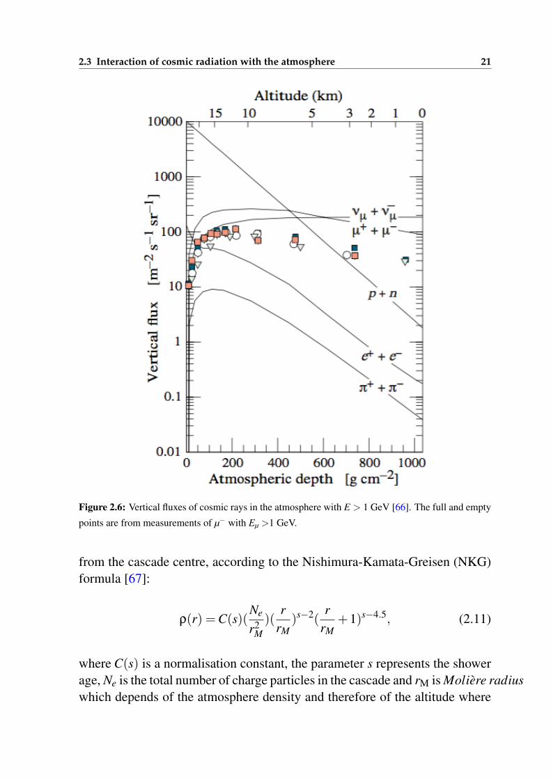
2.3 Interaction of cosmic radiation with the atmosphere 21

Figure 2.6: Vertical fluxes of cosmic rays in the atmosphere with E > 1 GeV [66]. The full and empty

points are from measurements of µ− with Eµ >1 GeV.

from the cascade centre, according to the Nishimura-Kamata-Greisen (NKG)formula [67]:

ρ(r) =C(s)(Ne

r2M)(

rrM

)s−2(r

rM+1)s−4.5, (2.11)

where C(s) is a normalisation constant, the parameter s represents the showerage, Ne is the total number of charge particles in the cascade and rM is Moliere radiuswhich depends of the atmosphere density and therefore of the altitude where

22 Cosmic rays

the cascade is measured:

rM =Es

EcX0 (2.12)

Here Es =√

4π

αmec2 = 21.2 MeV is a constant depending on the particle mass,

and X0 is the atmospheric fraction unit traversed by the particle. At the sealevel rM ≈78 m, and increases with the altitude as the air density decreases.The NKG formula is valid for 0.6 ≤ s ≤ 1.8 and 0.01 ≤ r

rM≤ 10. Finally the

lateral extension of the cascade is dominated by the Coulomb scattering of lowenergy electrons and is also characterised by the Moliere radius.

It is important to take into account some fluctuations occurring during EASdevelopment, even for particles with the same primary mass and energy. Theaverage relationship between the cascade size Ne and its primary energy E0depends on the depth in the atmosphere. The equation 2.13 is an estimate ofthis relationship for primaries with 1014 < E < 1017 eV at 965 m above thesea level (920 g cm−2) [68].

E0 ∼ 3.9×106 GeV (Ne/106)0.9 (2.13)

The shower maximum (on average) moves down into the atmosphere as E0increases. At the maximum shower development there are only 2/3 particlesper primary energy unit.

Electrons and positrons are the most abundant particles in the cascade,while the number of muons produced by charged meson decays (Eq. 2.5) is ofone order of magnitude less. The lateral development of the EAS gives rise toa large cascade extent at ground level reaching to about several kilometres forthe high primary energies.

The number of muons in the EAS, per square meter, as function of thelateral distance from the cascade centre was proposed by Greisen in 1960 [67](Eq. 2.14):

ρµ =C(1r0)1.25·Nµ·r−0.75(1− 1

r0)−0.25, (2.14)

where r is the lateral distance, r0 is is the characteristic enlargement distance,Nµ is the total number of muons in the shower and C is a normalisation con-stant. The dispersion of the muonic component is due to both, the transversemomentum of pions and kaons which generate muons and to the Coulombscattering.

2.4 Cosmic radiation at surface 23

2.4 Cosmic radiation at surface

Muons are the charge particles more abundant at sea level. Most of muonsare produced at 15 Km of altitude and they loose about 2 GeV by ionizationbefore reaching the ground. For muon energies lower than 1 GeV the energyspectrum is almost flat, gradually steepening to reflect the primary spectrum inthe 10 – 100 GeV range. A further steepening occurs at higher energies, untilthe critical energies of pions and kaons (επ = 115 GeV and εK = 850 GeV)since almost all mesons decay such that the muon flux has the same power lawof parent mesons. At energies above critical values, pions and kaons tend tointeract in the atmosphere before they decay. At larger energies (Eµ1 TeV)the atmospheric muon spectrum can be described by a power law. The integralintensity of vertical muons above 1 GeV/c at sea level is≈70 m−2s−1sr−1 [69,70]. The overall angular distribution of muons at surface level scales withcos2 θ (Eµ ∼3 GeV). At lower energy the angular distribution increasinglysteeps, while at higher energy it flattens approaching a secθ distribution forEµ επ and θ < 60 [71].

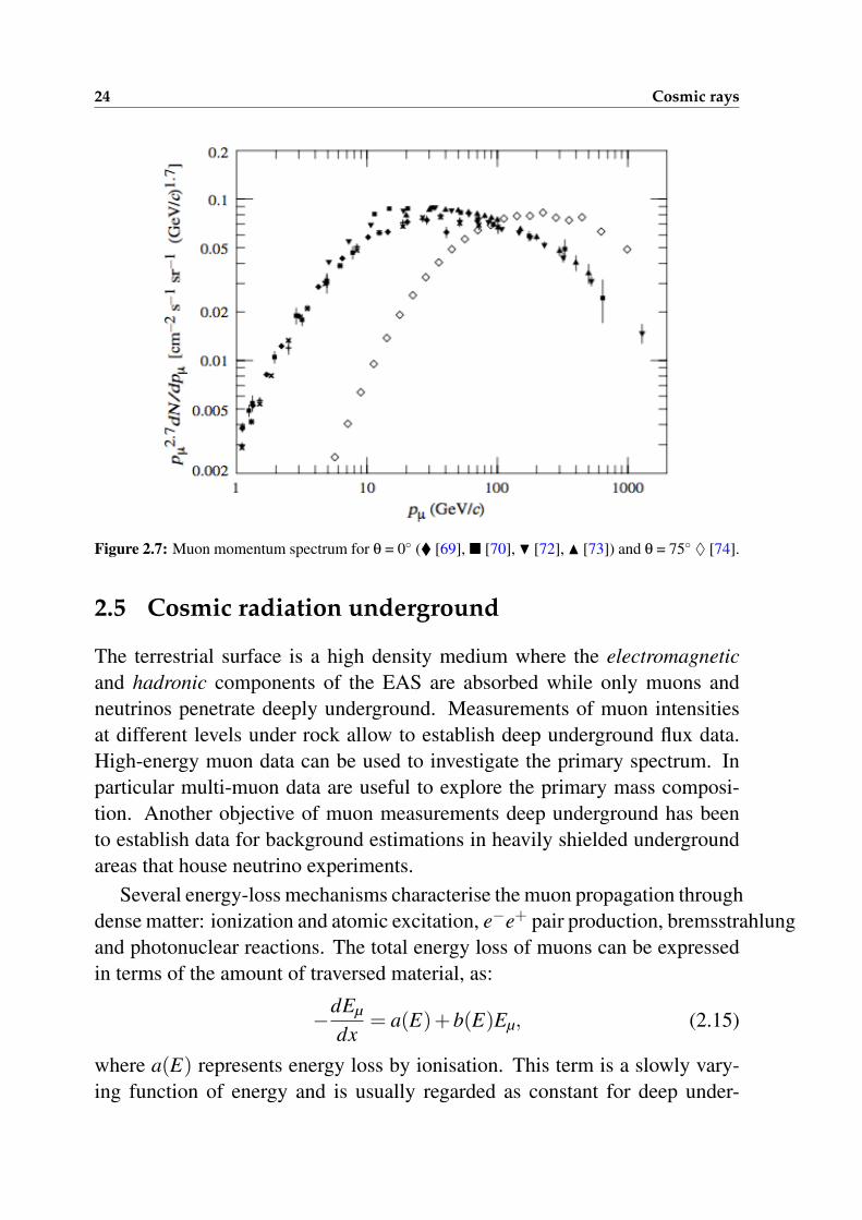
Figure 2.7 shows the muon momentum spectrum at sea level for two θ

values, measured by different experiments. At large θ, low energy muonsdecay before reaching the surface whereas high energy pions decay beforethey interact, thus the average muon energy increases.

By other hand, the µ+/µ− ratio reflects the π+ excess over π− as well asthe K+ excess over K− in the forward fragmentation region of proton initiatedinteractions. The larger amount of protons over the neutrons in the primaryspectrum is also reflected in the µ+/µ− ratio.

The electromagnetic component of the EAS at ground level consists ofelectrons, positrons and photons mostly produced in the cascades generatedby the decay of charge and neutral mesons. The muon decay is the mainsource of low energy electrons at sea level. The integral vertical intensity ofelectrons plus positrons is ≈ 30, 6 and 0.2 m−2s−1sr−1 above 10, 100 and1000 MeV respectively at sea level, but the exact numbers depend sensitivelyon the altitude, and the angular dependence is complex because of the depen-dence of the different electron sources with the altitude. The ratio of photonsto the sum of electrons and positrons is ≈ 1.3 above 1 GeV and 0.7 below thecritical energy ε0 (∼80 MeV in air) [75].

24 Cosmic rays

Figure 2.7: Muon momentum spectrum for θ = 0 ( [69], [70], H [72], N [73]) and θ = 75 ♦ [74].

2.5 Cosmic radiation underground

The terrestrial surface is a high density medium where the electromagneticand hadronic components of the EAS are absorbed while only muons andneutrinos penetrate deeply underground. Measurements of muon intensitiesat different levels under rock allow to establish deep underground flux data.High-energy muon data can be used to investigate the primary spectrum. Inparticular multi-muon data are useful to explore the primary mass composi-tion. Another objective of muon measurements deep underground has beento establish data for background estimations in heavily shielded undergroundareas that house neutrino experiments.

Several energy-loss mechanisms characterise the muon propagation throughdense matter: ionization and atomic excitation, e−e+ pair production, bremsstrahlungand photonuclear reactions. The total energy loss of muons can be expressedin terms of the amount of traversed material, as:

−dEµ

dx= a(E)+b(E)Eµ, (2.15)

where a(E) represents energy loss by ionisation. This term is a slowly vary-ing function of energy and is usually regarded as constant for deep under-

2.5 Cosmic radiation underground 25

ground applications. The term b(E) is the fraction of energy loss by radia-tive processes: bremsstrahlung, pair production and photo-nuclear reactions.The quantity ε = a/b defines a critical value of energy, below which the ion-isation loss is more important than the radiative processes. In case of rockε≈500 GeV. Parameters a(E) and b(E) are quite sensitive to the chemicalcomposition of the rock. For this reason it is very important to perform acareful study of the rock for every position of the experimental location.

The detailed knowledge of energy-loss mechanisms is important to com-pute the range-energy relation. The relation between the muon spectrum atsurface and the spectra at different underground depths can be determinedwith the consequent depth-intensity definition. The latter is a method to ex-plore the highest energies of the muon spectrum at ground level and to link itwith the primary spectrum and composition of cosmic rays.

If we integrate the equation 2.15 by assuming a(E) as a constant, the aver-age range can be obtained,

Rµ(E) =1b

lna+bE

a(2.16)

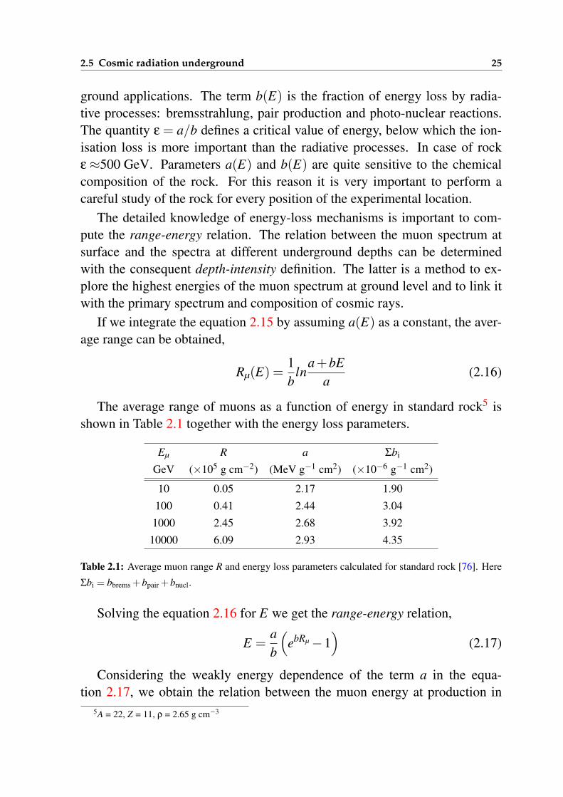
The average range of muons as a function of energy in standard rock5 isshown in Table 2.1 together with the energy loss parameters.

Eµ R a Σbi

GeV (×105 g cm−2) (MeV g−1 cm2) (×10−6 g−1 cm2)

10 0.05 2.17 1.90

100 0.41 2.44 3.04

1000 2.45 2.68 3.92

10000 6.09 2.93 4.35

Table 2.1: Average muon range R and energy loss parameters calculated for standard rock [76]. Here

Σbi = bbrems +bpair +bnucl.

Solving the equation 2.16 for E we get the range-energy relation,

E =ab

(ebRµ−1

)(2.17)

Considering the weakly energy dependence of the term a in the equa-tion 2.17, we obtain the relation between the muon energy at production in

5A = 22, Z = 11, ρ = 2.65 g cm−3

26 Cosmic rays

the atmosphere (Eµ,0) and its mean energy (Eµ) after have traversed a thick-ness X of the rock (water or ice) as follows,

Eµ = (Eµ,0 +ab)e−bX − a

b(2.18)

Monte Carlo simulations of the underground muon propagation should ac-count for the stochastic energy-loss processes, which play an important rolewhen the muon range starts to be comparable to the radiation length in themedium. Large fluctuations are produced at large depths (high energies) wherethe electromagnetic processes (accounted by the term b) are more importantthan the energy loss by ionization.

There are two depth regimes for equation 2.18. For bX1, Eµ,0≈Eµ(X)+

aX , while for bX1, Eµ,0≈ (ε+Eµ(X))exp(bX). Thus, at shallow depths thedifferential muon energy spectrum is approximately constant for Eµ < aX andsteepens to reflect the surface muon spectrum for Eµ > aX , whereas for bX > 1the differential spectrum underground is again constant for low muon energiesbut steepens to reflect the surface spectrum for Eµ > ε≈ 0.5 TeV. In the deepregime the shape is independent of depth, although the intensity decreasesexponentially with depth. In general the muon spectrum at slant depth X is

dNµ(X)

dEµ=

dNµ

dEµ,0

dEµ,0

dEµ=

dNµ

dEµ,0e−bX , (2.19)

where Eµ,0 is the solution of the equation 2.18 in the approximation of neglect-ing fluctuations.

2.6 Cosmic radiation measurements

The flux of primary cosmic rays is attenuated with increasing atmosphericdepth. Light primary nuclei reach larger atmospheric depths, while heavy pri-mary nuclei are rapidly attenuated because of fragmentation. The interactionmean free path of nuclei in air decreases from 75 g/cm2 for protons to 14g/cm2 for iron nuclei. Thus, the flux of primary nuclei that survive on theirway through the atmosphere down to the sea level is vanishing small.

Direct measurements

The high altitude data detected with direct measurements, are the backbonefor the determination of primary cosmic ray spectrum and mass composition

2.6 Cosmic radiation measurements 27

over a wide range of energies. Direct measurements may access cosmic rayenergies in different intervals up to ∼ 1015 eV, and are complemented withEAS data at high and ultra-high energies. Detailed simulations and cross-calibrations between different types of detectors are necessary to establish theprimary energy spectrum from air shower experiments.

The low energy component of cosmic rays hitting the atmosphere, has beenexplored in the top atmosphere with instruments on board of satellites, spacestations, aircrafts and balloons using a wide variety of techniques and instru-ments. Excellent data between the geomagnetic cutoff and 1015 eV, havebeen produced by experiments in the upper atmosphere using electronic de-tectors such as spectrometers, Cherenkov counters, calorimeters, transitiondetectors, combinations of the more advanced systems, or nuclear emulsions,thus recording and identifying individual primary cosmic rays. One of the ad-vantages of direct measurements is the possibility of identifying the originalparticle that would generate the EAS detected by ground-based detector. How-ever, to increase the maximum detectable energy it is needed to have detectorsbig enough, and to perform long measurements, which becomes an importantdifficulty that this type of experiments have to overcome. The use of nu-clear emulsion chambers has been pioneered by experiments like JACEE6[77]and RUNJOB7 [78], which have studied the energy spectra of cosmic raysfrom proton to iron at energies extending to 1015 eV. The nuclear emulsionis a passive technique with limited exposure times because of the integratingeffects of the background. Several new complex balloon-borne instrumentsemploying superconducting magnets were built like BESS8, CAPRICE9, andHEAT10 [79–81], whereas data from cosmic rays with a large charge range andhigher energies have been covered by balloon-borne instruments which havebeen equipped with efficient spectrometers like ATIC11 [82] and CREAM 12

[83]. These instruments are characterized by a high energy resolution, espe-cially CREAM with the larger number of pixels in smaller area allowing avery efficient geometry. It reached a record of exposure of 162 days, being 40days in only one flight. As part of the direct measurements of primary cosmic

6 Japanesse-American Cooperative Emulsion Experiment7 RUssia-Nippon JOint Balloon collaboration8 Balloon-Eexperiment with a Supercondinting Solenoid9 Cosmic AntiParticle Ring-Imaging Cherenkov Experiment

10 High-Energy Antimatter Telescope11 Advanced Think Ionization Calorimeter12 Cosmic Ray Energetic and Mass Balloon Experiment

28 Cosmic rays

rays, in 2006 was launched the satellite based experiment PAMELA13 [84],which is a permanent magnet spectrometer with a variety of specialised de-tectors, dedicated to perform precision measurements of cosmic rays, mainlyfocussed on particle identification and to study the antimatter component ofcosmic radiation.

Air shower measurements

With the increasing energy, at values larger than 1014 eV, the differential fluxof primary cosmic rays rapidly falls to one particle per square meter-steradianper year (see figure 2.1). This leads to use larger collection areas with detec-tors operating for long periods in order to reach reasonable statistics. Hencethe understanding of the primary flux at energies around the knee depends onground-based air shower observations, and require the detection of differentcomponents of the EAS, i.e. hadrons, electromagnetic radiation, Cherenkovlight and muon content. At this point, only secondary products from air show-ers can be measured. These particle showers are spread over large areas deepin the atmosphere, at ground level and even underground.

Air shower experiments that use the atmosphere as a calorimeter generallymeasure a quantity that is related to total energy per particle. As explained insections 2.2 and 2.4 electrons and positrons are the most abundant particles inthe cascade, while muons are the charge particles more abundant at see level.Many experiments have been dedicated to detect the air shower componentsin order to investigate the spectrum and composition of primary cosmic raysfacing the problem of the low event rate at high energies with large installa-tions. They consist of large detector arrays at ground level with different alti-tudes with respect to the sea level. Relevant data of the cosmic ray spectrumat energies around the knee have been reported by shower experiments likeEAS-TOP, EAS-TOP/MACRO, KASCADE, KASCADE-GRANDE, MSU,TUNKA, SPASE/AMANDA, CASAMIA, TIBET and IceCube experiments,between others [5, 12, 37–46, 85, 86]. Some of the most relevant results aboutthe chemical composition in the energy range around the knee of the primarycosmic ray spectrum have been obtained by the KASCADE experiment inKarlsruhe, which is optimised to measure EAS in the energy range of 1014 eVto 1017 eV. It consists of a big scintillator array with muon tracking detectors,which was projected to distinguish between muons and electrons, and a huge

13 Payload for Antimatter Matter Exploration and Light-nuclei Astophysics

2.6 Cosmic radiation measurements 29

iron sampling calorimeter installed at centre of KASCADE detector aimed tomeasure energy and number of hadrons. Different components of the EAS canbe measured by using this multi-detector concept. This complex experimentalarrange is spread over an area of 200×200 m2 located at 110 meters above thesea level. KASCADE-GRANDE is an extension of KASCADE, and consistsof a multi-component air shower experiment aimed to measure the all-particleenergy spectrum by extending the energy region to 1018 eV and with a largercollection area of 700×700 m2.

Other shower experiments have also explored different kinematic regionsof the cosmic ray spectrum and have made useful contributions in researchesabout the elemental composition. The EAS-TOP experiment, located at 2005m above the sea level operated in the ninetieth at the Gran Sasso Labora-tories producing important results about the flux of various primary cosmicray elements and the all-particle energy spectrum in the range of 1015 eV to1016 eV. Some results come from measurements in coincidence between thesurface apparatus EAS-TOP with the underground detector MACRO, whichis located under the mountainous overburden of the Gran Sasso in Italy. Inthe same decade, in Chicago and Michigan began operating the experimentCASA-MIA whose objective was studying gamma rays and cosmic ray inter-actions above 1014 eV. CASA-MIA was based on an array of surface particledetectors (CASA) and another array of underground muon detectors (MIA).Data from CASA-MIA allowed to estimate a position and shape of the kneefrom the electron and muon size of individual showers, slightly above 1015 eVand suggested that the knee is dominated by heavy elements. Similar resultswere obtained by the shower array TIBET experiment in China.

Experiments which study cosmic rays at higher energies (E > 1016 eV)complement the shower arrays that work around the knee energy. Such is thecase of KASCADE-GRANDE, HiRes14, AGASA15 and the AUGER experi-ments. HiRes was mainly based on the fluorescence technique with opticaltelescopes [87], AGASA is a ground-level array of muon detectors cover-ing 100 Km2, while Auger employs ground array and fluorescence detectionmethods. Cosmic rays of high and ultra-high energies (up to 1018 eV andbeyond) have been measured by these experiments, through the measurementof its shower components. They have also confirmed the knee and observed

14 High Resolution Fly’s Eye15 Akeno Giant Air Shower Array

30 Cosmic rays

the GZK cutoff (briefly introduced in section 2.2.4) at the second knee of thespectrum as an indication of the highest energy cosmic rays interacting withthe cosmic microwave background [35, 88–91].

Underground measurements

The secondary particles generated during the EAS evolution down to the groundlevel are absorbed in interactions with the rock, while only muons penetratesdeeply underground. Muon intensities have been measured at different under-ground levels with a varying amount of overburden rock, down to depths ofabout 106 g cm−2, as well as in ice to shallower depths. At underground levelthe advantage is the possibility of measuring only the muonic component ofthe EAS. Underground measurements of muons have been carried out under avariety of different conditions, using different detector types, geometries, anddifferent rock compositions. Underwater measurements have the advantagethat the overburden is exactly known leaving no ambiguities about densityand composition variations along a particle trajectory.

Among the most relevant underground measurements, that have measuredmuon multiplicity distribution to explore the energy spectrum and composi-tion of cosmic rays, we should mention the MACRO 16 experiment at Labo-ratory Nazionali del Gran Sasso (LNGS) which is took data from 1989 until2001 and consisted of large liquid scintillator counters, streamer tubes andplastic track-etch detectors. This is one of the deeper detectors (3.2 ×105 gcm−2), collecting muons with a threshold energy of ∼1.4 TeV. In the sameinstitute (LNGS) another underground experiment, the LVD 17, was installed,consisting of 38 modules each containing eight liquid scintillator counters.Both, LVD and MACRO, registered events in coincidence with the surfaceexperiment EAS-TOP which covers an area approximately 105 m2 [92, 93].EAS-TOP was used to measure the electromagnetic size of the shower Ne,whereas the muon multiplicity was measured with its underground facility. Inaddition, detector SOUDAN II [94] from Minnesota obtained a muon multi-plicity distribution, corresponding to a muon threshold Eth = 700 GeV. Thisis a calorimeter consisting of iron/drift tubes located at a depth of 2.1×105

g cm−2. At a shallower depth (8.5×104 g cm−2) was installed the BUST18

16 Monopole with Astrophysics and Cosmic Ray Observatory17 Large Volume Detector18 Baksan Underground Scintillation Telescope

2.6 Cosmic radiation measurements 31

detector [95], an underground scintillator telescope consisting of an array offour horizontal and for vertical scintillator layers, to detect muons over 220GeV which has reconstructed the energy spectrum of cosmic rays at about1012 eV [96]. More recently started the experiment EMMA19, which is 85 munderground and differs from other underground experiments in its ability tomeasure lateral distribution of muons [97]. Many of these experiments useddifferent Monte Carlo hadronic-interaction models to simulate the shower, andGEANT to propagate muons through the rock. Their results suggested the ex-istence of the knee and were consistent with an mixed chemical compositionhaving an increasing mass trend at energies around the knee. The inaccuraciesof the hadronic interaction models and accumulated systematic uncertaintieswere the main limits.

19 Experiment with Multi Muon Aray

3Cosmic ray physics with accelerator

detectors

During the era of LEP [17], the particle accelerator built at CERN in Genevaand used from 1989 until 2000, some experiments started to develop a com-mon cosmic-ray research project called Cosmo-LEP [98], taking advantageof the relative shallow depth location and making use of the performance andgood tracking capabilities of these underground detectors. The participatingdetectors were ALEPH1, DELPHI2 and L3 + C. Another accelerator baseddetector that have performed studies of atmospheric muons is CMS3 [99], oneof the four large experiments at CERN LHC at present.

In the following, the most relevant results related to atmospheric muonmeasurements in accelerator-based detectors at CERN are presented.

3.1 Cosmo-ALEPH experiment

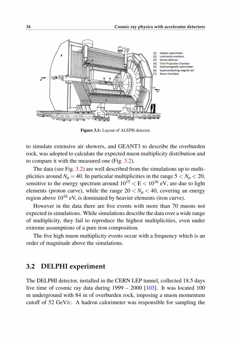
Cosmo-ALEPH [100] was the first experiment to operate in Cosmo-LEP project.The ALEPH apparatus, located 140 m underground, was capable to detectmuons with threshold energy Eth= 70 GeV and record multi-muon events withmultiplicities up to 150 muons in an area of∼8 m2. The ALEPH location wasthe deepest LEP point. It collected 580 000 cosmic ray events during LEPdata taking periods during 1997 - 1999, corresponding to 19.6 days effectivetime [101]. The TPC of ALEPH with 1.8 m outer radius, surrounded by theelectromagnetic (ECAL) and hadronic (HCAL) calorimeters (Fig. 3.1) insidea magnet field of 1.5 T, provided good tracking capabilities. Cosmic triggerwas given by the the coincidence of energy deposition of muons in oppositeHCAL supermodules.

A Monte Carlo strategy using CORSIKA with QGSJET 01 model [102]

1 Apparatus for LEP PHysics2 DEtector with Lepton Photon and Hadron Identification3 Compact Muon Solenoid

33

34 Cosmic ray physics with accelerator detectors

Figure 3.1: Layout of ALEPH detector.

to simulate extensive air showers, and GEANT3 to describe the overburdenrock, was adopted to calculate the expected muon multiplicity distribution andto compare it with the measured one (Fig. 3.2).

The data (see Fig. 3.2) are well described from the simulations up to multi-plicities around Nµ = 40. In particular multiplicities in the range 5 < Nµ < 20,sensitive to the energy spectrum around 1015 < E < 1016 eV, are due to lightelements (proton curve), while the range 20 < Nµ < 40, covering an energyregion above 1016 eV, is dominated by heavier elements (iron curve).

However in the data there are five events with more than 70 muons notexpected in simulations. While simulations describe the data over a wide rangeof multiplicity, they fail to reproduce the highest multiplicities, even underextreme assumptions of a pure iron composition.

The five high muon multiplicity events occur with a frequency which is anorder of magnitude above the simulations.

3.2 DELPHI experiment

The DELPHI detector, installed in the CERN LEP tunnel, collected 18.5 dayslive time of cosmic ray data during 1999 – 2000 [103]. It was located 100m underground with 84 m of overburden rock, imposing a muon momentumcutoff of 52 GeV/c. A hadron calorimeter was responsible for sampling the

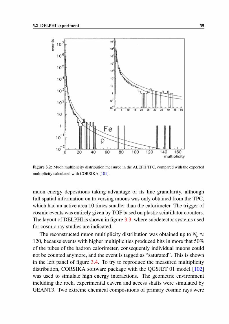
3.2 DELPHI experiment 35

Figure 3.2: Muon multiplicity distribution measured in the ALEPH TPC, compared with the expected

multiplicity calculated with CORSIKA [101].

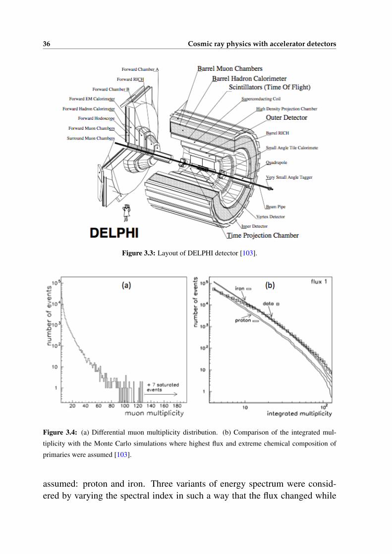
muon energy depositions taking advantage of its fine granularity, althoughfull spatial information on traversing muons was only obtained from the TPC,which had an active area 10 times smaller than the calorimeter. The trigger ofcosmic events was entirely given by TOF based on plastic scintillator counters.The layout of DELPHI is shown in figure 3.3, where subdetector systems usedfor cosmic ray studies are indicated.

The reconstructed muon multiplicity distribution was obtained up to Nµ ≈120, because events with higher multiplicities produced hits in more that 50%of the tubes of the hadron calorimeter, consequently individual muons couldnot be counted anymore, and the event is tagged as “saturated”. This is shownin the left panel of figure 3.4. To try to reproduce the measured multiplicitydistribution, CORSIKA software package with the QGSJET 01 model [102]was used to simulate high energy interactions. The geometric environmentincluding the rock, experimental cavern and access shafts were simulated byGEANT3. Two extreme chemical compositions of primary cosmic rays were

36 Cosmic ray physics with accelerator detectors

Figure 3.3: Layout of DELPHI detector [103].

Figure 3.4: (a) Differential muon multiplicity distribution. (b) Comparison of the integrated mul-

tiplicity with the Monte Carlo simulations where highest flux and extreme chemical composition of

primaries were assumed [103].

assumed: proton and iron. Three variants of energy spectrum were consid-ered by varying the spectral index in such a way that the flux changed while

3.3 L3 + C experiment 37

the shape was kept. The measured integrated4 multiplicity distribution wascompared with Monte Carlo simulations (right panel of figure 3.4).

The high muon multiplicity events, in DELPHI, were defined as those withmore than 45 muons. They concluded that the Monte Carlo simulation basedon the hadronic interaction model QGSJET failed to describe the abundanceof high multiplicity events, despite of using the combination of extreme as-sumptions of highest measured flux values and pure iron spectrum [103].

3.3 L3 + C experiment

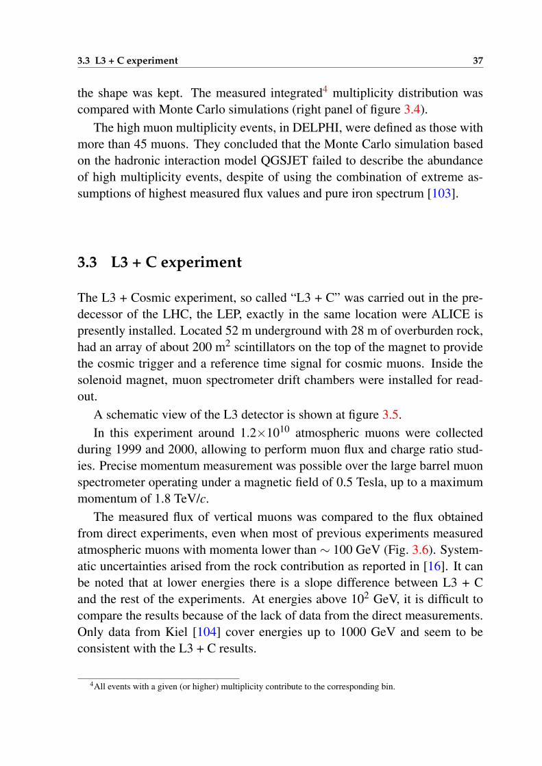
The L3 + Cosmic experiment, so called “L3 + C” was carried out in the pre-decessor of the LHC, the LEP, exactly in the same location were ALICE ispresently installed. Located 52 m underground with 28 m of overburden rock,had an array of about 200 m2 scintillators on the top of the magnet to providethe cosmic trigger and a reference time signal for cosmic muons. Inside thesolenoid magnet, muon spectrometer drift chambers were installed for read-out.

A schematic view of the L3 detector is shown at figure 3.5.In this experiment around 1.2×1010 atmospheric muons were collected

during 1999 and 2000, allowing to perform muon flux and charge ratio stud-ies. Precise momentum measurement was possible over the large barrel muonspectrometer operating under a magnetic field of 0.5 Tesla, up to a maximummomentum of 1.8 TeV/c.

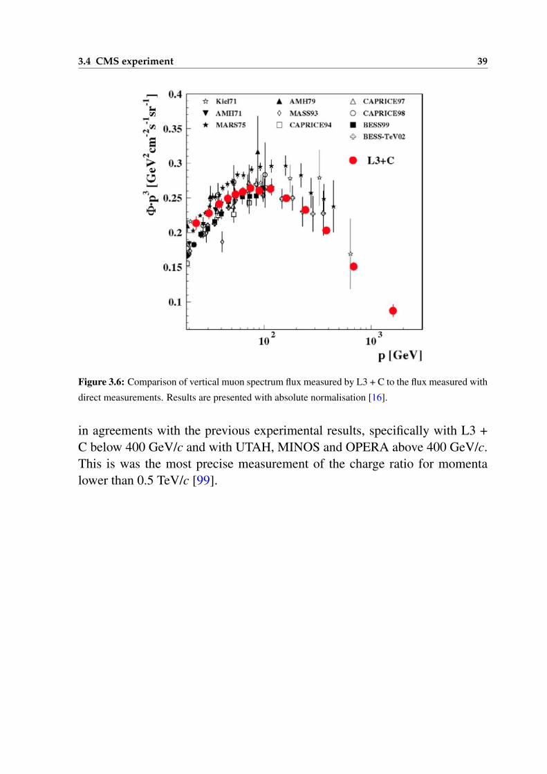
The measured flux of vertical muons was compared to the flux obtainedfrom direct experiments, even when most of previous experiments measuredatmospheric muons with momenta lower than ∼ 100 GeV (Fig. 3.6). System-atic uncertainties arised from the rock contribution as reported in [16]. It canbe noted that at lower energies there is a slope difference between L3 + Cand the rest of the experiments. At energies above 102 GeV, it is difficult tocompare the results because of the lack of data from the direct measurements.Only data from Kiel [104] cover energies up to 1000 GeV and seem to beconsistent with the L3 + C results.

4All events with a given (or higher) multiplicity contribute to the corresponding bin.

38 Cosmic ray physics with accelerator detectors

Figure 3.5: Layout of L3 detector.

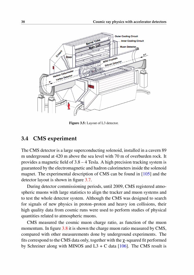
3.4 CMS experiment

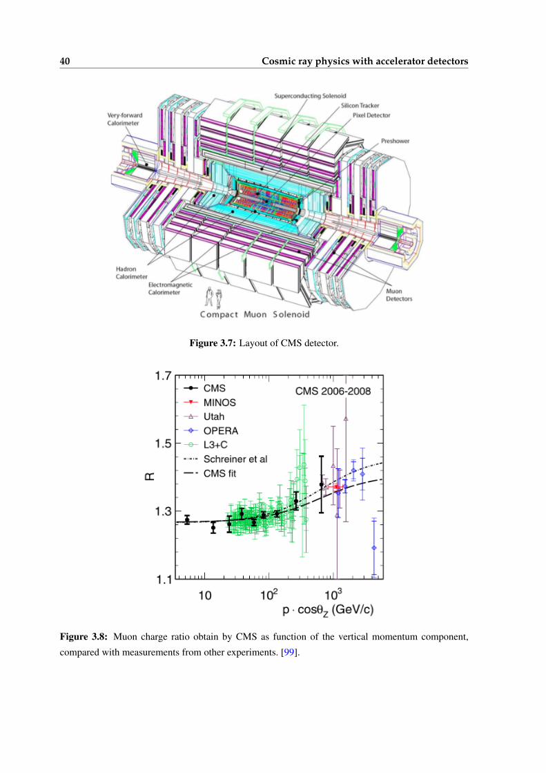
The CMS detector is a large superconducting solenoid, installed in a cavern 89m underground at 420 m above the sea level with 70 m of overburden rock. Itprovides a magnetic field of 3.8 – 4 Tesla. A high precision tracking system isguaranteed by the electromagnetic and hadron calorimeters inside the solenoidmagnet. The experimental description of CMS can be found in [105] and thedetector layout is shown in figure 3.7.

During detector commissioning periods, until 2009, CMS registered atmo-spheric muons with large statistics to align the tracker and muon systems andto test the whole detector system. Although the CMS was designed to searchfor signals of new physics in proton–proton and heavy ion collisions, theirhigh quality data from cosmic runs were used to perform studies of physicalquantities related to atmospheric muons.

CMS measured the cosmic muon charge ratio, as function of the muonmomentum. In figure 3.8 it is shown the charge muon ratio measured by CMS,compared with other measurements done by underground experiments. Thefits correspond to the CMS data only, together with the χ-squared fit performedby Schreiner along with MINOS and L3 + C data [106]. The CMS result is

3.4 CMS experiment 39

Figure 3.6: Comparison of vertical muon spectrum flux measured by L3 + C to the flux measured with

direct measurements. Results are presented with absolute normalisation [16].

in agreements with the previous experimental results, specifically with L3 +C below 400 GeV/c and with UTAH, MINOS and OPERA above 400 GeV/c.This is was the most precise measurement of the charge ratio for momentalower than 0.5 TeV/c [99].

40 Cosmic ray physics with accelerator detectors

Figure 3.7: Layout of CMS detector.

Figure 3.8: Muon charge ratio obtain by CMS as function of the vertical momentum component,

compared with measurements from other experiments. [99].

4The ALICE experiment at CERN

ALICE (A Large Ion Collider Experiment) [1] is one of the four large exper-iments at the CERN Large Hadron Collider. It was designed to study Quark-Gluon Plasma (QGP) formation in ultra-relativistic heavy-ion collisions at theCERN Large Hadron Collider (LHC). It is focused on the strongly interactingmatter at extreme energy densities, predicted by quantum chromodynamicsand whose existence is now firmly established experimentally [2]. The physicsprogram is based on the A–A (Pb–Pb) collisions. It also includes proton–proton (pp) and proton–nucleus (p–Pb) collisions in order to vary the energydensity and interaction volume to provide the reference data for the heavy-ionprogramme. ALICE has been optimised to reach high-momentum resolutionas well as excellent particle identification over a broad range of momentumfrom tens of MeV/c to around 100 GeV/c, up to the highest multiplicitiespredicted by the LHC. ALICE employs essentially all known particle iden-tification techniques: specific ionization energy loss dE/dx, time–of–flight,transition and Cerenkov radiation, electromagnetic calorimetry, muon filtersand topological decay reconstruction.

The large size and excellent tracking capability of the ALICE Time Projec-tion Chamber allowed to perform atmospheric muon analysis in order to con-tribute to cosmic ray physics. With this aim a programme of cosmic ray datataking was carried out, during pauses in collider operations where no beamwas circulating. This is intended to be an extension of earlier cosmic-ray stud-ies with high-energy physics detectors, pioneered by ALEPH, DELPHI andL3 (see Chapter 3). Now, in the LHC, experiments can operate under stableconditions for many years.

In this Chapter, a brief overview of the ALICE detector is described, withemphasis in detector subsystems directly involved in the cosmic-ray studiesperformed in this thesis.

41

42 The ALICE experiment at CERN

4.1 Brief picture of the ALICE detector system

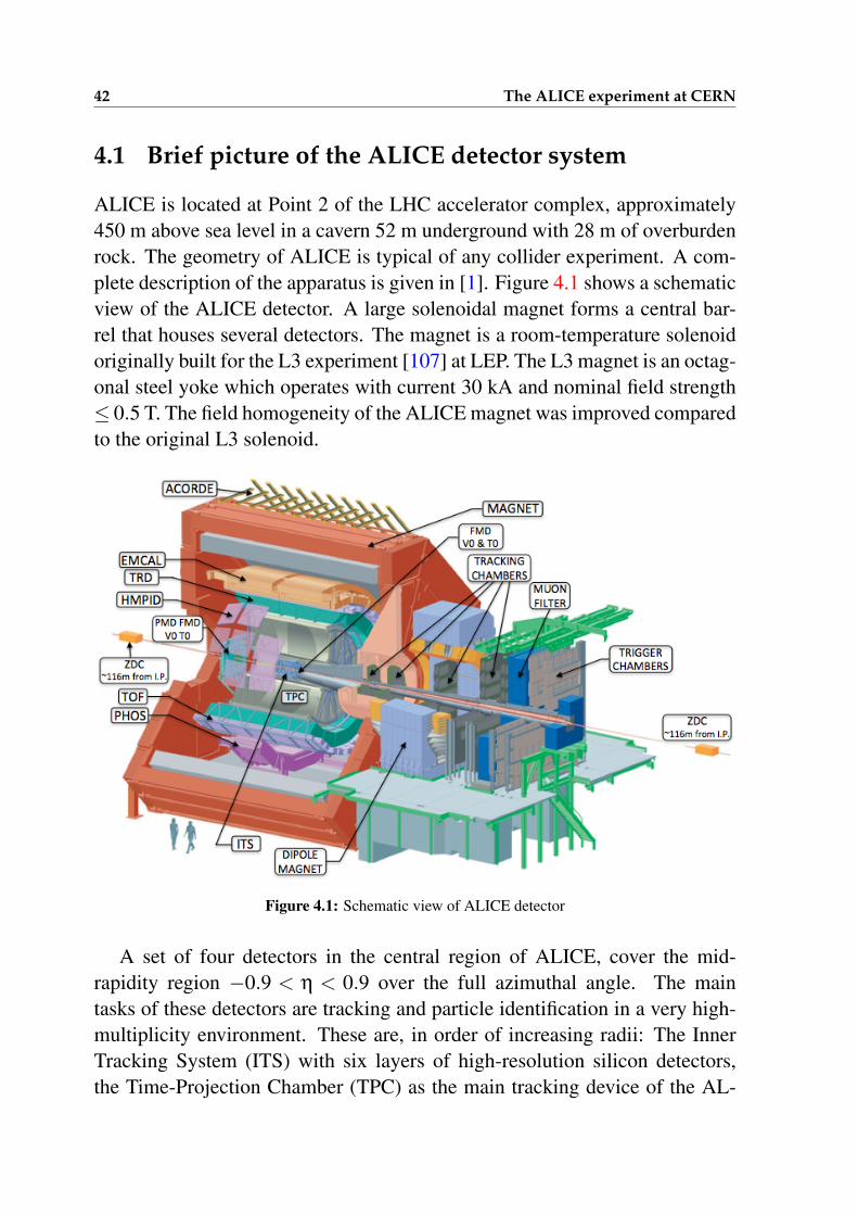
ALICE is located at Point 2 of the LHC accelerator complex, approximately450 m above sea level in a cavern 52 m underground with 28 m of overburdenrock. The geometry of ALICE is typical of any collider experiment. A com-plete description of the apparatus is given in [1]. Figure 4.1 shows a schematicview of the ALICE detector. A large solenoidal magnet forms a central bar-rel that houses several detectors. The magnet is a room-temperature solenoidoriginally built for the L3 experiment [107] at LEP. The L3 magnet is an octag-onal steel yoke which operates with current 30 kA and nominal field strength≤ 0.5 T. The field homogeneity of the ALICE magnet was improved comparedto the original L3 solenoid.

Figure 4.1: Schematic view of ALICE detector

A set of four detectors in the central region of ALICE, cover the mid-rapidity region −0.9 < η < 0.9 over the full azimuthal angle. The maintasks of these detectors are tracking and particle identification in a very high-multiplicity environment. These are, in order of increasing radii: The InnerTracking System (ITS) with six layers of high-resolution silicon detectors,the Time-Projection Chamber (TPC) as the main tracking device of the AL-

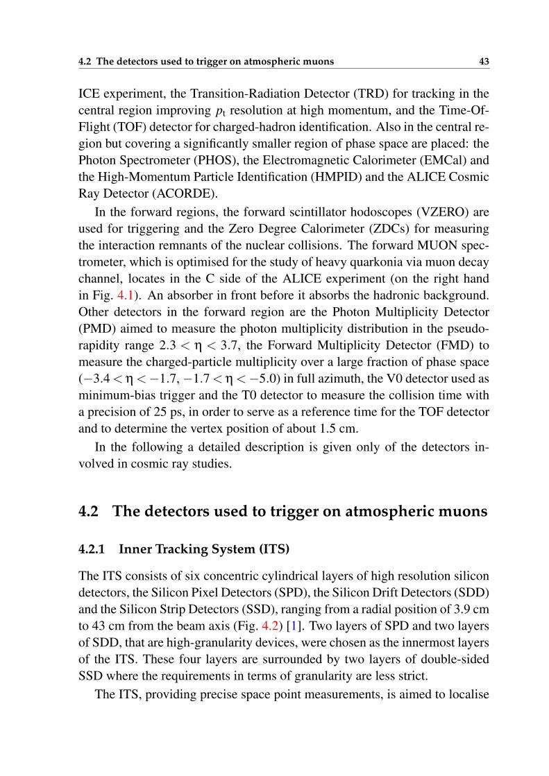
4.2 The detectors used to trigger on atmospheric muons 43

ICE experiment, the Transition-Radiation Detector (TRD) for tracking in thecentral region improving pt resolution at high momentum, and the Time-Of-Flight (TOF) detector for charged-hadron identification. Also in the central re-gion but covering a significantly smaller region of phase space are placed: thePhoton Spectrometer (PHOS), the Electromagnetic Calorimeter (EMCal) andthe High-Momentum Particle Identification (HMPID) and the ALICE CosmicRay Detector (ACORDE).

In the forward regions, the forward scintillator hodoscopes (VZERO) areused for triggering and the Zero Degree Calorimeter (ZDCs) for measuringthe interaction remnants of the nuclear collisions. The forward MUON spec-trometer, which is optimised for the study of heavy quarkonia via muon decaychannel, locates in the C side of the ALICE experiment (on the right handin Fig. 4.1). An absorber in front before it absorbs the hadronic background.Other detectors in the forward region are the Photon Multiplicity Detector(PMD) aimed to measure the photon multiplicity distribution in the pseudo-rapidity range 2.3 < η < 3.7, the Forward Multiplicity Detector (FMD) tomeasure the charged-particle multiplicity over a large fraction of phase space(−3.4 < η <−1.7,−1.7 < η <−5.0) in full azimuth, the V0 detector used asminimum-bias trigger and the T0 detector to measure the collision time witha precision of 25 ps, in order to serve as a reference time for the TOF detectorand to determine the vertex position of about 1.5 cm.

In the following a detailed description is given only of the detectors in-volved in cosmic ray studies.

4.2 The detectors used to trigger on atmospheric muons

4.2.1 Inner Tracking System (ITS)

The ITS consists of six concentric cylindrical layers of high resolution silicondetectors, the Silicon Pixel Detectors (SPD), the Silicon Drift Detectors (SDD)and the Silicon Strip Detectors (SSD), ranging from a radial position of 3.9 cmto 43 cm from the beam axis (Fig. 4.2) [1]. Two layers of SPD and two layersof SDD, that are high-granularity devices, were chosen as the innermost layersof the ITS. These four layers are surrounded by two layers of double-sidedSSD where the requirements in terms of granularity are less strict.

The ITS, providing precise space point measurements, is aimed to localise

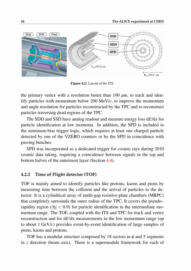
44 The ALICE experiment at CERN

Figure 4.2: Layout of the ITS.

the primary vertex with a resolution better than 100 µm, to track and iden-tify particles with momentum below 200 MeV/c, to improve the momentumand angle resolution for particles reconstructed by the TPC and to reconstructparticles traversing dead regions of the TPC.

The SDD and SSD have analog readout and measure energy loss dE/dx forparticle identification at low momenta. In addition, the SPD is included inthe minimum-bias trigger logic, which requires at least one charged particledetected by one of the VZERO counters or by the SPD in coincidence withpassing bunches.

SPD was incorporated as a dedicated trigger for cosmic rays during 2010cosmic data taking, requiring a coincidence between signals in the top andbottom halves of the outermost layer (Section 4.4).

4.2.2 Time of Flight detector (TOF)

TOF is mainly aimed to identify particles like protons, kaons and pions bymeasuring time between the collision and the arrival of particles to the de-tector. It is a cylindrical array of multi-gap resistive-plate chambers (MRPC)that completely surrounds the outer radius of the TPC. It covers the pseudo–rapidity region (|η| < 0.9) for particle identification in the intermediate mo-mentum range. The TOF, coupled with the ITS and TPC for track and vertexreconstruction and for dE/dx measurements in the low momentum range (upto about 1 GeV/c) provides event-by-event identification of large samples ofpions, kaons and protons.

TOF has a modular structure composed by 18 sectors in φ and 5 segmentsin z direction (beam axis). There is a supermodule framework for each of

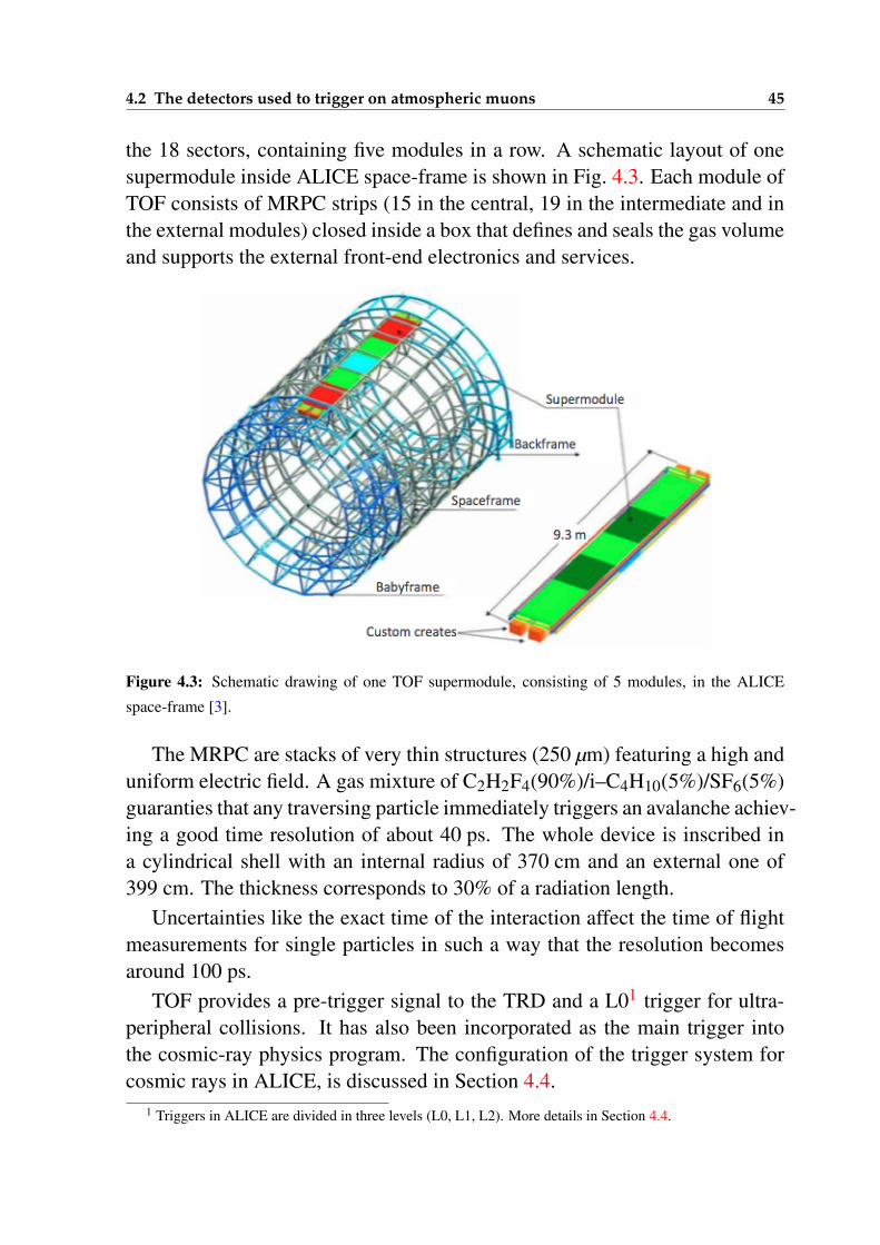
4.2 The detectors used to trigger on atmospheric muons 45

the 18 sectors, containing five modules in a row. A schematic layout of onesupermodule inside ALICE space-frame is shown in Fig. 4.3. Each module ofTOF consists of MRPC strips (15 in the central, 19 in the intermediate and inthe external modules) closed inside a box that defines and seals the gas volumeand supports the external front-end electronics and services.

Figure 4.3: Schematic drawing of one TOF supermodule, consisting of 5 modules, in the ALICE

space-frame [3].

The MRPC are stacks of very thin structures (250 µm) featuring a high anduniform electric field. A gas mixture of C2H2F4(90%)/i–C4H10(5%)/SF6(5%)guaranties that any traversing particle immediately triggers an avalanche achiev-ing a good time resolution of about 40 ps. The whole device is inscribed ina cylindrical shell with an internal radius of 370 cm and an external one of399 cm. The thickness corresponds to 30% of a radiation length.

Uncertainties like the exact time of the interaction affect the time of flightmeasurements for single particles in such a way that the resolution becomesaround 100 ps.

TOF provides a pre-trigger signal to the TRD and a L01 trigger for ultra-peripheral collisions. It has also been incorporated as the main trigger intothe cosmic-ray physics program. The configuration of the trigger system forcosmic rays in ALICE, is discussed in Section 4.4.

1 Triggers in ALICE are divided in three levels (L0, L1, L2). More details in Section 4.4.

46 The ALICE experiment at CERN

4.2.3 The ALICE Cosmic Ray Detector (ACORDE)

The detector ACORDE provides the trigger setup configuration to detect cos-mic muons, as well as a spatial position when atmospheric muons hit theALICE magnet. It consists of an array of 60 scintillator modules located onthe three top octants of the ALICE magnet, covering 10% of its surface areaand has an azimuthal coverage of −60 < φ < 60 (Fig. 4.4).

Figure 4.4: Photograph of the ACORDE scintillator module array.

ACORDE has been a very important piece of ALICE providing L0 triggersignals when atmospheric muons impinge upon the ALICE detector. Thesefast signals have been used for commissioning, calibration and alignment pro-cedures of some of the ALICE central detectors.

A single ACORDE module consists of two plastic scintillator padless, eachwith active area of 188 x 20 cm2 and 10 mm thickness, plus two Photomulti-plier tubes (PMT) placed at the end of each scintillator. They are installed ontop of each other with the readout in coincidence.

Details of ACORDE as cosmic trigger are explained in Section 4.4.

4.3 The detector used to track cosmic muons

4.3.1 Time Projection Chamber (TPC)

The ALICE TPC is the largest detector of its type ever built. It is the maintracking detector of the central barrel and is optimised to provide, together

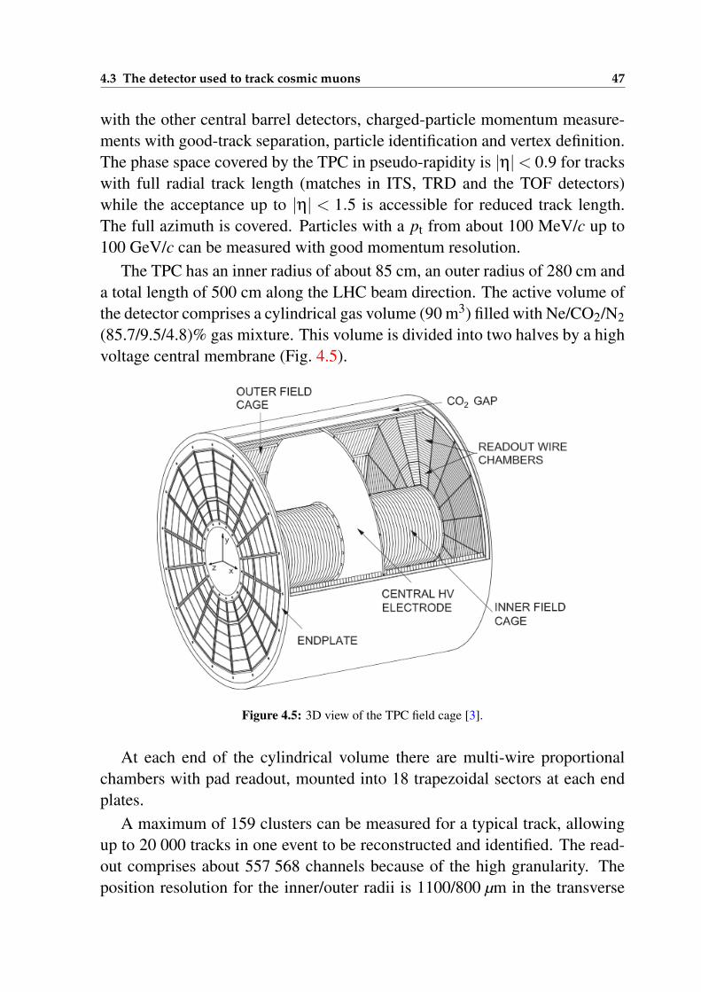
4.3 The detector used to track cosmic muons 47

with the other central barrel detectors, charged-particle momentum measure-ments with good-track separation, particle identification and vertex definition.The phase space covered by the TPC in pseudo-rapidity is |η|< 0.9 for trackswith full radial track length (matches in ITS, TRD and the TOF detectors)while the acceptance up to |η| < 1.5 is accessible for reduced track length.The full azimuth is covered. Particles with a pt from about 100 MeV/c up to100 GeV/c can be measured with good momentum resolution.

The TPC has an inner radius of about 85 cm, an outer radius of 280 cm anda total length of 500 cm along the LHC beam direction. The active volume ofthe detector comprises a cylindrical gas volume (90 m3) filled with Ne/CO2/N2(85.7/9.5/4.8)% gas mixture. This volume is divided into two halves by a highvoltage central membrane (Fig. 4.5).

Figure 4.5: 3D view of the TPC field cage [3].

At each end of the cylindrical volume there are multi-wire proportionalchambers with pad readout, mounted into 18 trapezoidal sectors at each endplates.

A maximum of 159 clusters can be measured for a typical track, allowingup to 20 000 tracks in one event to be reconstructed and identified. The read-out comprises about 557 568 channels because of the high granularity. Theposition resolution for the inner/outer radii is 1100/800 µm in the transverse

48 The ALICE experiment at CERN

plane and 1250/1100 µs along the beam axis. The charge collected at the endplate is proportional to the energy loss of particles in the gas mixture. TheTPC is the slowest detector in ALICE, being its drift time equal to 94 µs. Thisis important to be taken into account for the trigger, because once an event isaccepted, no other event is measured with the TPC within the next 94 µs.

The use of TPC to reconstruct the trajectories of cosmic muons traversingthe active volume of the detector is explained in Section 5.1.

4.4 Trigger system for cosmic rays in ALICE

The trigger system

Three detector subsystems were used to provide dedicated triggers to study themuonic component of extensive air showers from cosmic rays: TOF [108],ACORDE [109] and SPD [110]. They were used, in combination with theALICE TPC to collect single atmospheric muons and muon bundles in orderto study high-energy cosmic rays in the region of the knee (3×1015 eV) ofthe cosmic ray spectrum.

The trigger architecture of ALICE consists of two main steps: the low-leveltrigger is a hardware trigger called Central Trigger Processor (CTP) and theHigh-Level Trigger (HLT) is implemented as a pure software trigger [111].The CTP is related with the readout, and combines inputs from different de-tector subsystems. The HLT receives a copy of the data read out from eachsubdetector and processes it. The CTP combines the trigger signals of thevarious subdetectors to decide if an event is accepted, in which case its infor-mation is written to disk to be processed by the HLT.

In ALICE there are 3 trigger levels (L0, L1, L2) and for each of them 2 sub-levels are present: sub-level b meaning before vetoes and sub-level a meaningafter vetoes. The three trigger levels reduce the event rate depending on theinput signals. The first level L0 is delivered after 1.2 µs, the second level L1after 6.5 µs, and the final trigger signal L2 is delivered after 100 µs, uponcompletion of the drift time in the TPC. Only after a L2 trigger the event isfinally stored. In particular L0b gives the number of times a given trigger isfired, while L2a gives the number of times the same trigger passes the CTPdecision as well as the detector dead time and any other vetoes. These triggerscalers and in particular the ratio L2a/L0b gives the estimate of the live time

4.4 Trigger system for cosmic rays in ALICE 49

of the detectors for the specific trigger used.The ALICE “cosmic” trigger detectors provide fast L0 signals to the CTP,

when atmospheric muons hit the ALICE detector. Consequently the CTP pro-cesses and synchronises the information from trigger detectors and sends thecorrect sequences of trigger signals to all detectors to perform the readout ofrelevant events. Besides of providing multi-coincidence trigger signals, cos-mic trigger detectors store kinematic information from atmospheric muons.This system was configured to select atmospheric muons with zenithal anglesbetween 0 and 60, and azimuthal angles from 0 to 360.

TOF as the main trigger

The ALICE TOF detector is a fast-response device, well suited for triggeringpurposes. It requires a signal in a pad corresponding to a cluster of readoutchannels covering an area of 500 cm2 in the upper part of the detector andanother signal in a pad in the opposite lower part forming a back-to-back co-incidence (OB0) with respect to the central axis of the detector. With a back-to-back coincidence the trigger rate is higher than 10 Hz. The configurationof the pads involved in the trigger can be changed via software. In some pe-riods of data taking, this flexibility has been exploited to require a signal inan upper pad and in the opposing pad plus the two adjacent pads forming aback-to-back±1 coincidence (OB1), which gives rise to a better trigger rateallowing to register higher muon multiplicities. The OB3 configuration con-sists of a back-to-back±3 coincidence and allows to reach a rate of ∼70-80Hz. Two of the three trigger configurations implemented in our data sample(OB0 and OB3) are illustrated in the first panel (a) of figure 4.6.

ACORDE

ACORDE have been traditionally used as “cosmic” trigger for alignment andcalibration purposes of the ALICE central detectors, thus becoming a veryimportant trigger detector for cosmic-ray studies. The trigger ACORDE wasformed by the coincidence of signals in two different modules (a two-fold co-incidence), although the trigger can also be configured to select events whena single module fires or when more than two modules fire (a n-fold coinci-dence). The rate of a single hit is about 100 Hz while the obtained rate for

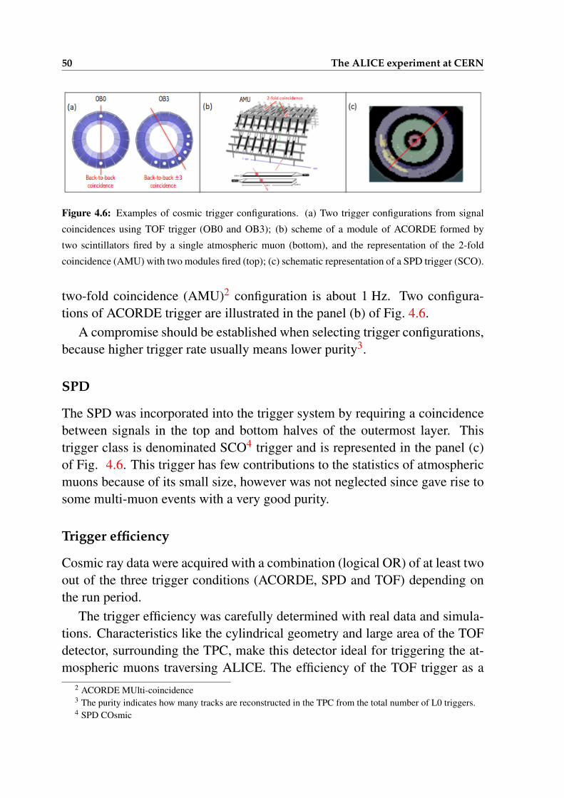
50 The ALICE experiment at CERN

Figure 4.6: Examples of cosmic trigger configurations. (a) Two trigger configurations from signal

coincidences using TOF trigger (OB0 and OB3); (b) scheme of a module of ACORDE formed by

two scintillators fired by a single atmospheric muon (bottom), and the representation of the 2-fold

coincidence (AMU) with two modules fired (top); (c) schematic representation of a SPD trigger (SCO).

two-fold coincidence (AMU)2 configuration is about 1 Hz. Two configura-tions of ACORDE trigger are illustrated in the panel (b) of Fig. 4.6.

A compromise should be established when selecting trigger configurations,because higher trigger rate usually means lower purity3.

SPD

The SPD was incorporated into the trigger system by requiring a coincidencebetween signals in the top and bottom halves of the outermost layer. Thistrigger class is denominated SCO4 trigger and is represented in the panel (c)of Fig. 4.6. This trigger has few contributions to the statistics of atmosphericmuons because of its small size, however was not neglected since gave rise tosome multi-muon events with a very good purity.

Trigger efficiency

Cosmic ray data were acquired with a combination (logical OR) of at least twoout of the three trigger conditions (ACORDE, SPD and TOF) depending onthe run period.

The trigger efficiency was carefully determined with real data and simula-tions. Characteristics like the cylindrical geometry and large area of the TOFdetector, surrounding the TPC, make this detector ideal for triggering the at-mospheric muons traversing ALICE. The efficiency of the TOF trigger as a

2 ACORDE MUlti-coincidence3 The purity indicates how many tracks are reconstructed in the TPC from the total number of L0 triggers.4 SPD COsmic

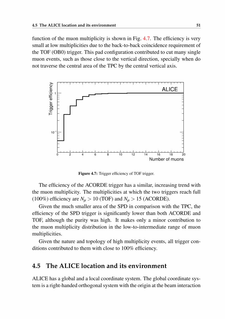
4.5 The ALICE location and its environment 51

function of the muon multiplicity is shown in Fig. 4.7. The efficiency is verysmall at low multiplicities due to the back-to-back coincidence requirement ofthe TOF (OB0) trigger. This pad configuration contributed to cut many singlemuon events, such as those close to the vertical direction, specially when donot traverse the central area of the TPC by the central vertical axis.

Number of muons0 2 4 6 8 10 12 14 16 18 20

Trig

ge

r e

ffic

ien

cy

1−10

1ALICE

Figure 4.7: Trigger efficiency of TOF trigger.

The efficiency of the ACORDE trigger has a similar, increasing trend withthe muon multiplicity. The multiplicities at which the two triggers reach full(100%) efficiency are Nµ > 10 (TOF) and Nµ > 15 (ACORDE).

Given the much smaller area of the SPD in comparison with the TPC, theefficiency of the SPD trigger is significantly lower than both ACORDE andTOF, although the purity was high. It makes only a minor contribution tothe muon multiplicity distribution in the low-to-intermediate range of muonmultiplicities.

Given the nature and topology of high multiplicity events, all trigger con-ditions contributed to them with close to 100% efficiency.

4.5 The ALICE location and its environment

ALICE has a global and a local coordinate system. The global coordinate sys-tem is a right-handed orthogonal system with the origin at the beam interaction

52 The ALICE experiment at CERN

point. The reconstruction softwares in ALICE use the local coordinate systemof the central tracking detectors. Both systems can be transformed one intoother by a simple rotation around the z axis.

In this work, with the purpose of studying cosmic rays, the global coordi-nate system of ALICE was adopted, in such a way that the z axis is alignedwith the LHC beam pipe (see figure 4.8) but the azimuthal and polar angleswere transformed in order to describe the arrival direction of atmosphericmuons. The cosmic–ray coordinate system can be defined as follows:

• origin of the system x = y = z = 0 at the nominal interaction point;

• the x–axis perpendicular to the local beam direction, aligned with thehorizontal mid-plane of the ALICE TPC, pointing towards the centre ofthe LHC;

• the y–axis perpendicular to the plane xz, pointing upwards;

• the z–axis parallel to the LHC beam pipe. Positive z axis points towardsside A (see Fig. 4.8);

• the azimuthal angle φ is measured at plane xz and increases clockwisefrom x (φ = 0) up to 360.

• the zenithal angle θ is measured with respect to the vertical y–axis andincreases from θ = 0 to θ = π/2

The ALICE environment

A detailed description of the ALICE experimental cavern plus the overbur-den rock, is used to reproduce the ALICE environment in our Monte Carlosimulations. Atmospheric muons arriving at the ALICE location experiencemeaningful physical effects due to the traversed material between the surfaceand the apparatus.

The ALICE detector is located 52 m underground, at Point 2 of the LHCaccelerator tunnel, in the commune of Saint Genis Pouilly, France. The surfacealtitude is 450 m above sea level. The location of the ALICE apparatus has28 m of overburden consisting of subalpine molasse rock. Only muons withan energy Eth, at the surface, larger than 16 GeV reach the detectors. Thecomposition of the rock is known from previous geological surveys carried

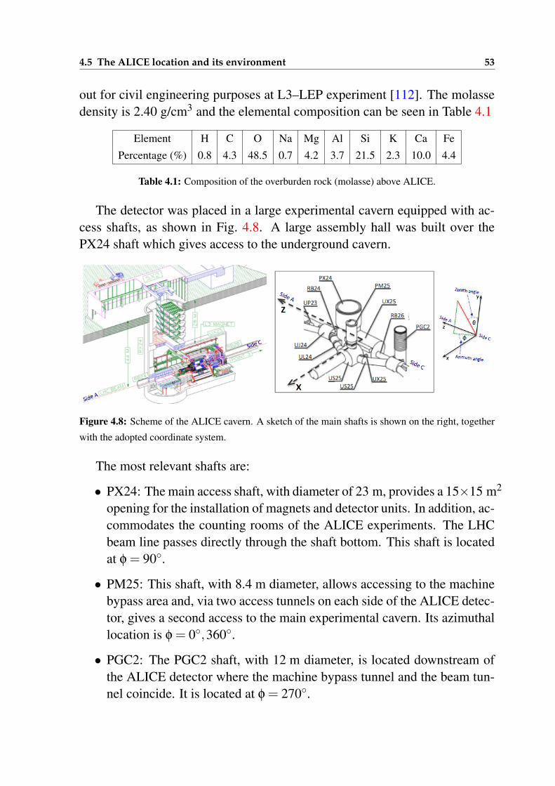
4.5 The ALICE location and its environment 53

out for civil engineering purposes at L3–LEP experiment [112]. The molassedensity is 2.40 g/cm3 and the elemental composition can be seen in Table 4.1

Element H C O Na Mg Al Si K Ca Fe

Percentage (%) 0.8 4.3 48.5 0.7 4.2 3.7 21.5 2.3 10.0 4.4

Table 4.1: Composition of the overburden rock (molasse) above ALICE.

The detector was placed in a large experimental cavern equipped with ac-cess shafts, as shown in Fig. 4.8. A large assembly hall was built over thePX24 shaft which gives access to the underground cavern.

Figure 4.8: Scheme of the ALICE cavern. A sketch of the main shafts is shown on the right, together

with the adopted coordinate system.

The most relevant shafts are:

• PX24: The main access shaft, with diameter of 23 m, provides a 15×15 m2

opening for the installation of magnets and detector units. In addition, ac-commodates the counting rooms of the ALICE experiments. The LHCbeam line passes directly through the shaft bottom. This shaft is locatedat φ = 90.

• PM25: This shaft, with 8.4 m diameter, allows accessing to the machinebypass area and, via two access tunnels on each side of the ALICE detec-tor, gives a second access to the main experimental cavern. Its azimuthallocation is φ = 0,360.

• PGC2: The PGC2 shaft, with 12 m diameter, is located downstream ofthe ALICE detector where the machine bypass tunnel and the beam tun-nel coincide. It is located at φ = 270.

5Event reconstruction

5.1 Atmospheric muon reconstruction

The ALICE TPC was used to reconstruct the trajectory of cosmic muons pass-ing through the active volume of the detector with full spatial information.Some of the most relevant characteristics are summarised in 4.3.1. For thepurpose of this thesis we exploited what we consider the main advantages ofthis detector: the excellent tracking capabilities.

The TPC, main tracking detector in the central barrel, provides the chargeparticle track reconstruction with a very good two-track separation. It was de-signed to detect particles stemming from the LHC beam collisions. However,there are differences between particles emerging from LHC beam collisionsand atmospheric muons traversing the TPC. A particle created in a collisionpasses very close to the centre of ALICE, and generates a track either in theupper half of the TPC or in the lower half. In contrast, an atmospheric muonvertically crosses the TPC, usually far from the central axis, and its track oftentraverses the whole length of the TPC.

5.1.1 Tracking algorithm

The TPC tracking algorithm [113], in the ALICE experiment, was designed toreconstruct tracks coming from the primary interaction vertex during the LHCbeam collisions. It follows the Kalman filter procedure [114] that allows tofind and fit tracks by working inwards from the outer radius of the detector,where, during collider operations, the track density is lower. According to theKalman filter, the propagation of track parameters like position, direction, cur-vature and its associate covariance matrix to the next pad row, is recursivelydone. The reconstructed tracks are conformed by specific clusters1. If a cluster

1 Particles interacting with the detector leave a signal in several adjacent space points or in several time binsof the detector. These signals are combined to form a cluster.

55

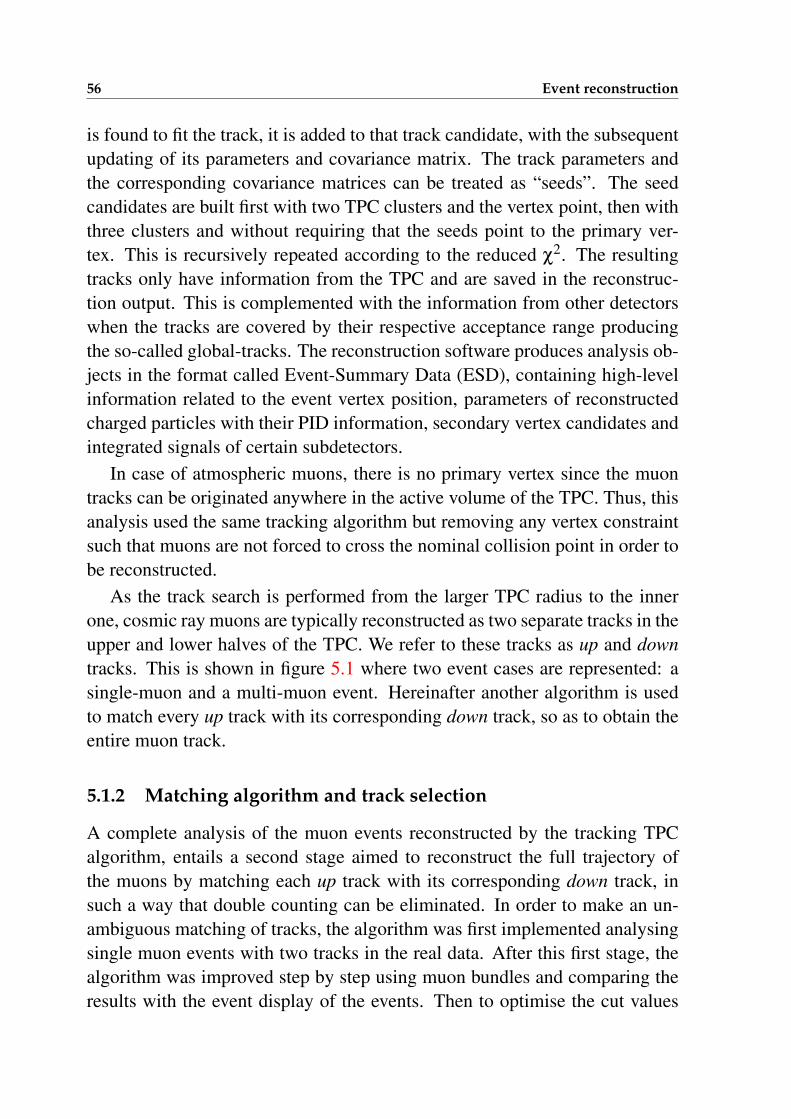
56 Event reconstruction

is found to fit the track, it is added to that track candidate, with the subsequentupdating of its parameters and covariance matrix. The track parameters andthe corresponding covariance matrices can be treated as “seeds”. The seedcandidates are built first with two TPC clusters and the vertex point, then withthree clusters and without requiring that the seeds point to the primary ver-tex. This is recursively repeated according to the reduced χ2. The resultingtracks only have information from the TPC and are saved in the reconstruc-tion output. This is complemented with the information from other detectorswhen the tracks are covered by their respective acceptance range producingthe so-called global-tracks. The reconstruction software produces analysis ob-jects in the format called Event-Summary Data (ESD), containing high-levelinformation related to the event vertex position, parameters of reconstructedcharged particles with their PID information, secondary vertex candidates andintegrated signals of certain subdetectors.

In case of atmospheric muons, there is no primary vertex since the muontracks can be originated anywhere in the active volume of the TPC. Thus, thisanalysis used the same tracking algorithm but removing any vertex constraintsuch that muons are not forced to cross the nominal collision point in order tobe reconstructed.

As the track search is performed from the larger TPC radius to the innerone, cosmic ray muons are typically reconstructed as two separate tracks in theupper and lower halves of the TPC. We refer to these tracks as up and downtracks. This is shown in figure 5.1 where two event cases are represented: asingle-muon and a multi-muon event. Hereinafter another algorithm is usedto match every up track with its corresponding down track, so as to obtain theentire muon track.

5.1.2 Matching algorithm and track selection

A complete analysis of the muon events reconstructed by the tracking TPCalgorithm, entails a second stage aimed to reconstruct the full trajectory ofthe muons by matching each up track with its corresponding down track, insuch a way that double counting can be eliminated. In order to make an un-ambiguous matching of tracks, the algorithm was first implemented analysingsingle muon events with two tracks in the real data. After this first stage, thealgorithm was improved step by step using muon bundles and comparing theresults with the event display of the events. Then to optimise the cut values

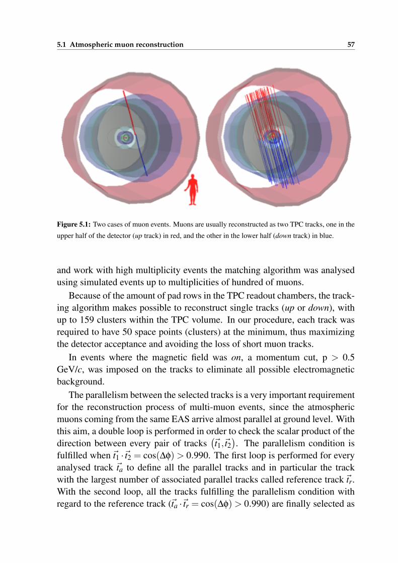
5.1 Atmospheric muon reconstruction 57

Figure 5.1: Two cases of muon events. Muons are usually reconstructed as two TPC tracks, one in the

upper half of the detector (up track) in red, and the other in the lower half (down track) in blue.

and work with high multiplicity events the matching algorithm was analysedusing simulated events up to multiplicities of hundred of muons.

Because of the amount of pad rows in the TPC readout chambers, the track-ing algorithm makes possible to reconstruct single tracks (up or down), withup to 159 clusters within the TPC volume. In our procedure, each track wasrequired to have 50 space points (clusters) at the minimum, thus maximizingthe detector acceptance and avoiding the loss of short muon tracks.

In events where the magnetic field was on, a momentum cut, p > 0.5GeV/c, was imposed on the tracks to eliminate all possible electromagneticbackground.

The parallelism between the selected tracks is a very important requirementfor the reconstruction process of multi-muon events, since the atmosphericmuons coming from the same EAS arrive almost parallel at ground level. Withthis aim, a double loop is performed in order to check the scalar product of thedirection between every pair of tracks

(~t1,~t2

). The parallelism condition is

fulfilled when ~t1 ·~t2 = cos(∆φ)> 0.990. The first loop is performed for everyanalysed track ~ta to define all the parallel tracks and in particular the trackwith the largest number of associated parallel tracks called reference track~tr.With the second loop, all the tracks fulfilling the parallelism condition withregard to the reference track (~ta ·~tr = cos(∆φ)> 0.990) are finally selected as

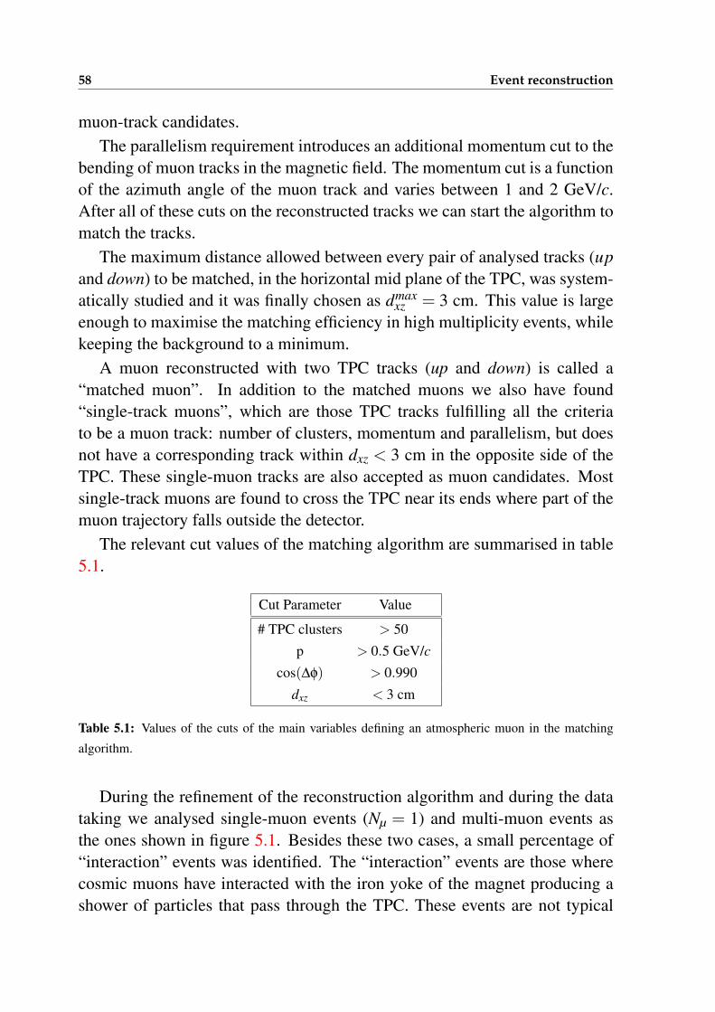
58 Event reconstruction

muon-track candidates.The parallelism requirement introduces an additional momentum cut to the

bending of muon tracks in the magnetic field. The momentum cut is a functionof the azimuth angle of the muon track and varies between 1 and 2 GeV/c.After all of these cuts on the reconstructed tracks we can start the algorithm tomatch the tracks.

The maximum distance allowed between every pair of analysed tracks (upand down) to be matched, in the horizontal mid plane of the TPC, was system-atically studied and it was finally chosen as dmax

xz = 3 cm. This value is largeenough to maximise the matching efficiency in high multiplicity events, whilekeeping the background to a minimum.

A muon reconstructed with two TPC tracks (up and down) is called a“matched muon”. In addition to the matched muons we also have found“single-track muons”, which are those TPC tracks fulfilling all the criteriato be a muon track: number of clusters, momentum and parallelism, but doesnot have a corresponding track within dxz < 3 cm in the opposite side of theTPC. These single-muon tracks are also accepted as muon candidates. Mostsingle-track muons are found to cross the TPC near its ends where part of themuon trajectory falls outside the detector.

The relevant cut values of the matching algorithm are summarised in table5.1.

Cut Parameter Value

# TPC clusters > 50

p > 0.5 GeV/c

cos(∆φ) > 0.990

dxz < 3 cm

Table 5.1: Values of the cuts of the main variables defining an atmospheric muon in the matching

algorithm.

During the refinement of the reconstruction algorithm and during the datataking we analysed single-muon events (Nµ = 1) and multi-muon events asthe ones shown in figure 5.1. Besides these two cases, a small percentage of“interaction” events was identified. The “interaction” events are those wherecosmic muons have interacted with the iron yoke of the magnet producing ashower of particles that pass through the TPC. These events are not typical

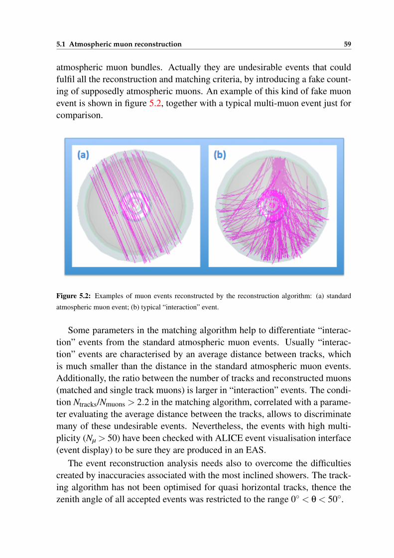
5.1 Atmospheric muon reconstruction 59

atmospheric muon bundles. Actually they are undesirable events that couldfulfil all the reconstruction and matching criteria, by introducing a fake count-ing of supposedly atmospheric muons. An example of this kind of fake muonevent is shown in figure 5.2, together with a typical multi-muon event just forcomparison.

Figure 5.2: Examples of muon events reconstructed by the reconstruction algorithm: (a) standard

atmospheric muon event; (b) typical “interaction” event.

Some parameters in the matching algorithm help to differentiate “interac-tion” events from the standard atmospheric muon events. Usually “interac-tion” events are characterised by an average distance between tracks, whichis much smaller than the distance in the standard atmospheric muon events.Additionally, the ratio between the number of tracks and reconstructed muons(matched and single track muons) is larger in “interaction” events. The condi-tion Ntracks/Nmuons > 2.2 in the matching algorithm, correlated with a parame-ter evaluating the average distance between the tracks, allows to discriminatemany of these undesirable events. Nevertheless, the events with high multi-plicity (Nµ > 50) have been checked with ALICE event visualisation interface(event display) to be sure they are produced in an EAS.

The event reconstruction analysis needs also to overcome the difficultiescreated by inaccuracies associated with the most inclined showers. The track-ing algorithm has not been optimised for quasi horizontal tracks, thence thezenith angle of all accepted events was restricted to the range 0 < θ < 50.

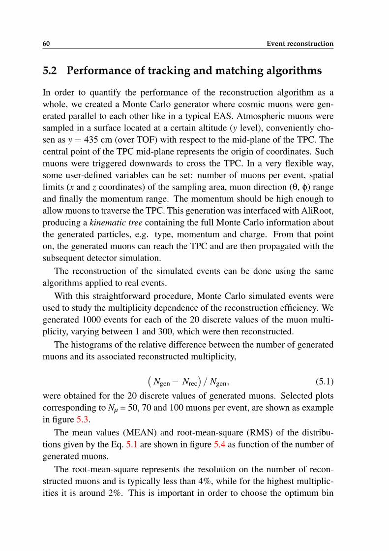
60 Event reconstruction

5.2 Performance of tracking and matching algorithms

In order to quantify the performance of the reconstruction algorithm as awhole, we created a Monte Carlo generator where cosmic muons were gen-erated parallel to each other like in a typical EAS. Atmospheric muons weresampled in a surface located at a certain altitude (y level), conveniently cho-sen as y = 435 cm (over TOF) with respect to the mid-plane of the TPC. Thecentral point of the TPC mid-plane represents the origin of coordinates. Suchmuons were triggered downwards to cross the TPC. In a very flexible way,some user-defined variables can be set: number of muons per event, spatiallimits (x and z coordinates) of the sampling area, muon direction (θ, φ) rangeand finally the momentum range. The momentum should be high enough toallow muons to traverse the TPC. This generation was interfaced with AliRoot,producing a kinematic tree containing the full Monte Carlo information aboutthe generated particles, e.g. type, momentum and charge. From that pointon, the generated muons can reach the TPC and are then propagated with thesubsequent detector simulation.

The reconstruction of the simulated events can be done using the samealgorithms applied to real events.

With this straightforward procedure, Monte Carlo simulated events wereused to study the multiplicity dependence of the reconstruction efficiency. Wegenerated 1000 events for each of the 20 discrete values of the muon multi-plicity, varying between 1 and 300, which were then reconstructed.

The histograms of the relative difference between the number of generatedmuons and its associated reconstructed multiplicity,(

Ngen− Nrec)/ Ngen, (5.1)

were obtained for the 20 discrete values of generated muons. Selected plotscorresponding to Nµ = 50, 70 and 100 muons per event, are shown as examplein figure 5.3.

The mean values (MEAN) and root-mean-square (RMS) of the distribu-tions given by the Eq. 5.1 are shown in figure 5.4 as function of the number ofgenerated muons.

The root-mean-square represents the resolution on the number of recon-structed muons and is typically less than 4%, while for the highest multiplic-ities it is around 2%. This is important in order to choose the optimum bin

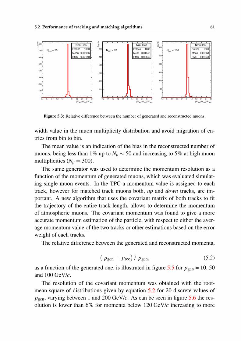
5.2 Performance of tracking and matching algorithms 61

NmuRes__4__1

Entries 1000

Mean 0.01216

RMS 0.01557

genN)/ recN­ genN(

0.5− 0.4− 0.3− 0.2− 0.1− 0 0.1 0.2 0.3 0.4 0.5

Counts

0

100

200

300

400

500

600

700

800

NmuRes__4__1

Entries 1000

Mean 0.01216

RMS 0.01557

NmuRes

Entries 1000

Mean 0.00986

RMS 0.02148

= 50genNNmuRes__5__2

Entries 1000

Mean 0.01624

RMS 0.0197

genN)/ recN­ genN(

0.5− 0.4− 0.3− 0.2− 0.1− 0 0.1 0.2 0.3 0.4 0.5C

ounts

0

100

200

300

400

500

600

NmuRes__5__2

Entries 1000

Mean 0.01624

RMS 0.0197

NmuRes

Entries 1000

Mean 0.01342

RMS 0.02045

= 70genNNmuRes__6__3

Entries 1000

Mean 0.01774

RMS 0.01772

genN)/ recN­ genN(

0.5− 0.4− 0.3− 0.2− 0.1− 0 0.1 0.2 0.3 0.4 0.5

Co

un

ts

0

100

200

300

400

500

600

NmuRes__6__3

Entries 1000

Mean 0.01774

RMS 0.01772

NmuRes

Entries 1000

Mean 0.01953

RMS 0.01948

= 100genN

Figure 5.3: Relative difference between the number of generated and reconstructed muons.

width value in the muon multiplicity distribution and avoid migration of en-tries from bin to bin.

The mean value is an indication of the bias in the reconstructed number ofmuons, being less than 1% up to Nµ ∼ 50 and increasing to 5% at high muonmultiplicities (Nµ = 300).

The same generator was used to determine the momentum resolution as afunction of the momentum of generated muons, which was evaluated simulat-ing single muon events. In the TPC a momentum value is assigned to eachtrack, however for matched track muons both, up and down tracks, are im-portant. A new algorithm that uses the covariant matrix of both tracks to fitthe trajectory of the entire track length, allows to determine the momentumof atmospheric muons. The covariant momentum was found to give a moreaccurate momentum estimation of the particle, with respect to either the aver-age momentum value of the two tracks or other estimations based on the errorweight of each tracks.

The relative difference between the generated and reconstructed momenta,(pgen− prec

)/ pgen, (5.2)

as a function of the generated one, is illustrated in figure 5.5 for pgen = 10, 50and 100 GeV/c.

The resolution of the covariant momentum was obtained with the root-mean-square of distributions given by equation 5.2 for 20 discrete values ofpgen, varying between 1 and 200 GeV/c. As can be seen in figure 5.6 the res-olution is lower than 6% for momenta below 120 GeV/c increasing to more

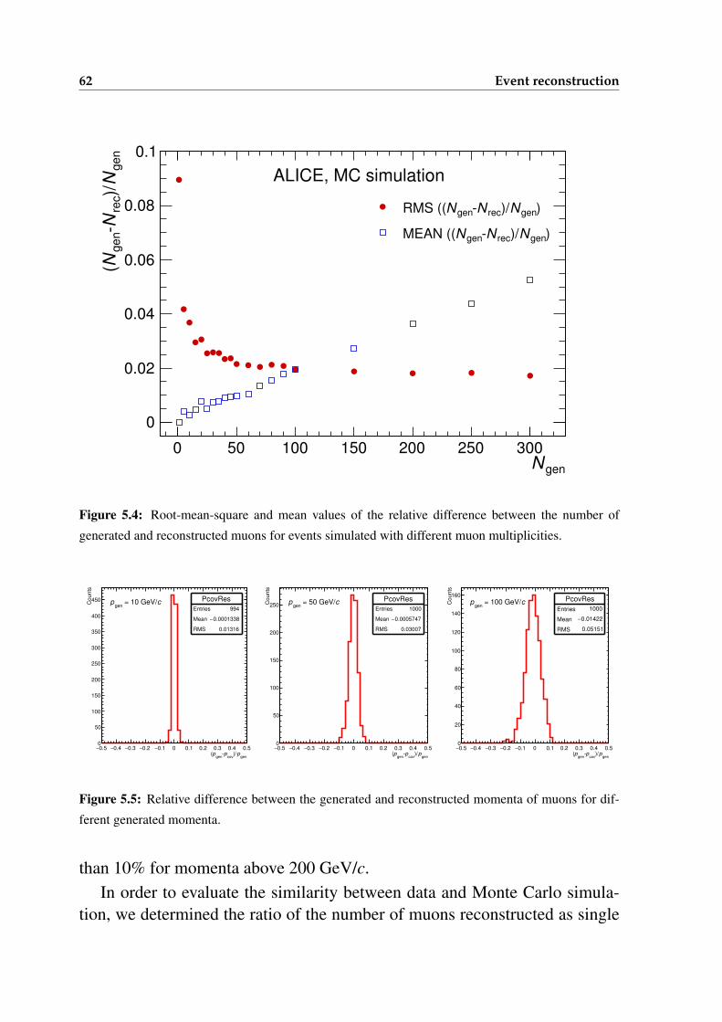
62 Event reconstruction

genN0 50 100 150 200 250 300

ge

nN

)/re

cN­

ge

nN(

0

0.02

0.04

0.06

0.08

0.1

)genN)/recN­genNRMS ((

)genN)/recN­genNMEAN ((

ALICE, MC simulation

Figure 5.4: Root-mean-square and mean values of the relative difference between the number of

generated and reconstructed muons for events simulated with different muon multiplicities.

genp)/

covp­

genp(

0.5− 0.4− 0.3− 0.2− 0.1− 0 0.1 0.2 0.3 0.4 0.5

Counts

0

50

100

150

200

250

300

350

400

450 PcovRes

Entries 994

Mean 0.0001338−

RMS 0.01316

c = 10 GeV/gen

p

genp)/

covp­

genp(

0.5− 0.4− 0.3− 0.2− 0.1− 0 0.1 0.2 0.3 0.4 0.5

Counts

0

50

100

150

200

250PcovRes

Entries 1000

Mean 0.0005747−

RMS 0.03007

c = 50 GeV/gen

p

genp)/

covp­

genp(

0.5− 0.4− 0.3− 0.2− 0.1− 0 0.1 0.2 0.3 0.4 0.5

Co

un

ts

0

20

40

60

80

100

120

140

160PcovRes

Entries 1000

Mean 0.01422−

RMS 0.05151

c = 100 GeV/gen

p

Figure 5.5: Relative difference between the generated and reconstructed momenta of muons for dif-

ferent generated momenta.

than 10% for momenta above 200 GeV/c.In order to evaluate the similarity between data and Monte Carlo simula-

tion, we determined the ratio of the number of muons reconstructed as single

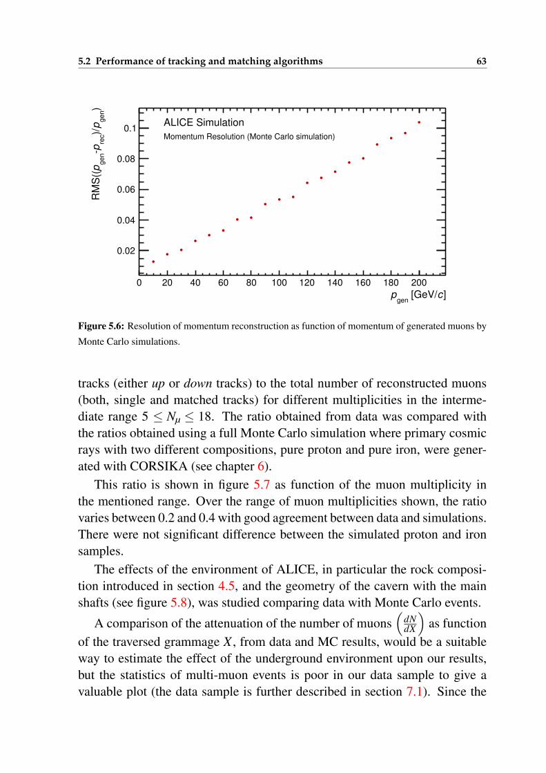
5.2 Performance of tracking and matching algorithms 63

]c [GeV/gen

p

0 20 40 60 80 100 120 140 160 180 200

)gen

p)/

rec

p­gen

pR

MS

((

0.02

0.04

0.06

0.08

0.1ALICE Simulation

Momentum Resolution (Monte Carlo simulation)

Figure 5.6: Resolution of momentum reconstruction as function of momentum of generated muons by

Monte Carlo simulations.

tracks (either up or down tracks) to the total number of reconstructed muons(both, single and matched tracks) for different multiplicities in the interme-diate range 5 ≤ Nµ ≤ 18. The ratio obtained from data was compared withthe ratios obtained using a full Monte Carlo simulation where primary cosmicrays with two different compositions, pure proton and pure iron, were gener-ated with CORSIKA (see chapter 6).

This ratio is shown in figure 5.7 as function of the muon multiplicity inthe mentioned range. Over the range of muon multiplicities shown, the ratiovaries between 0.2 and 0.4 with good agreement between data and simulations.There were not significant difference between the simulated proton and ironsamples.

The effects of the environment of ALICE, in particular the rock composi-tion introduced in section 4.5, and the geometry of the cavern with the mainshafts (see figure 5.8), was studied comparing data with Monte Carlo events.

A comparison of the attenuation of the number of muons(

dNdX

)as function

of the traversed grammage X , from data and MC results, would be a suitableway to estimate the effect of the underground environment upon our results,but the statistics of multi-muon events is poor in our data sample to give avaluable plot (the data sample is further described in section 7.1). Since the

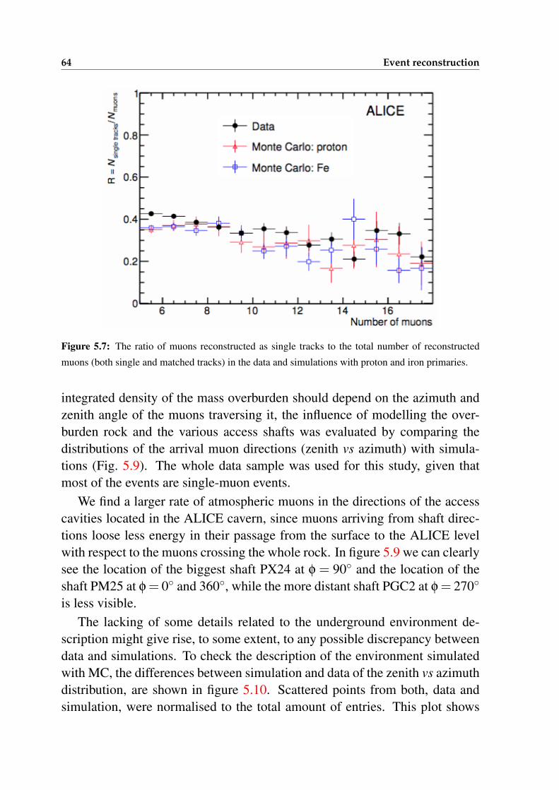
64 Event reconstruction

Figure 5.7: The ratio of muons reconstructed as single tracks to the total number of reconstructed

muons (both single and matched tracks) in the data and simulations with proton and iron primaries.

integrated density of the mass overburden should depend on the azimuth andzenith angle of the muons traversing it, the influence of modelling the over-burden rock and the various access shafts was evaluated by comparing thedistributions of the arrival muon directions (zenith vs azimuth) with simula-tions (Fig. 5.9). The whole data sample was used for this study, given thatmost of the events are single-muon events.

We find a larger rate of atmospheric muons in the directions of the accesscavities located in the ALICE cavern, since muons arriving from shaft direc-tions loose less energy in their passage from the surface to the ALICE levelwith respect to the muons crossing the whole rock. In figure 5.9 we can clearlysee the location of the biggest shaft PX24 at φ = 90 and the location of theshaft PM25 at φ = 0 and 360, while the more distant shaft PGC2 at φ = 270

is less visible.The lacking of some details related to the underground environment de-

scription might give rise, to some extent, to any possible discrepancy betweendata and simulations. To check the description of the environment simulatedwith MC, the differences between simulation and data of the zenith vs azimuthdistribution, are shown in figure 5.10. Scattered points from both, data andsimulation, were normalised to the total amount of entries. This plot shows

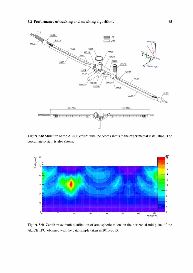
5.2 Performance of tracking and matching algorithms 65

Figure 5.8: Structure of the ALICE cavern with the access shafts to the experimental installation. The

coordinate system is also shown.

(degrees)φ0 50 100 150 200 250 300 350

(d

eg

ree

s)

θ

0

10

20

30

40

50

60

0

2

4

6

8

10

12

14

16

18

20

310×

Figure 5.9: Zenith vs azimuth distribution of atmospheric muons in the horizontal mid plane of the

ALICE TPC, obtained with the data sample taken in 2010-2013.

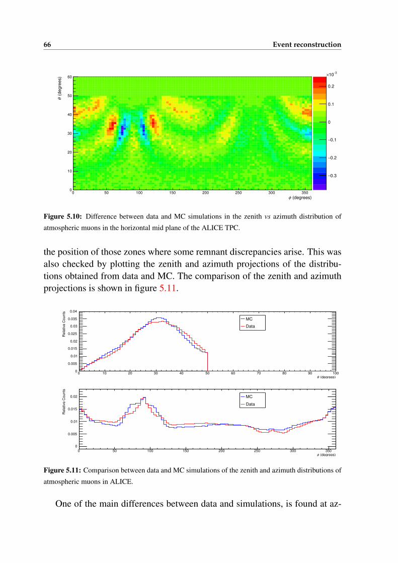
66 Event reconstruction

(degrees)φ0 50 100 150 200 250 300 350

(d

eg

ree

s)

θ

0

10

20

30

40

50

60

0.3−

0.2−

0.1−

0

0.1

0.2

3−10×

Figure 5.10: Difference between data and MC simulations in the zenith vs azimuth distribution of

atmospheric muons in the horizontal mid plane of the ALICE TPC.

the position of those zones where some remnant discrepancies arise. This wasalso checked by plotting the zenith and azimuth projections of the distribu-tions obtained from data and MC. The comparison of the zenith and azimuthprojections is shown in figure 5.11.

(degrees)θ0 10 20 30 40 50 60 70 80 90 100

Re

lative

Co

un

ts

0

0.005

0.01

0.015

0.02

0.025

0.03

0.035

0.04

MC

Data

(degrees)φ0 50 100 150 200 250 300 350

Re

lative

Co

un

ts

0

0.005

0.01

0.015

0.02 MC

Data

Figure 5.11: Comparison between data and MC simulations of the zenith and azimuth distributions of

atmospheric muons in ALICE.

One of the main differences between data and simulations, is found at az-

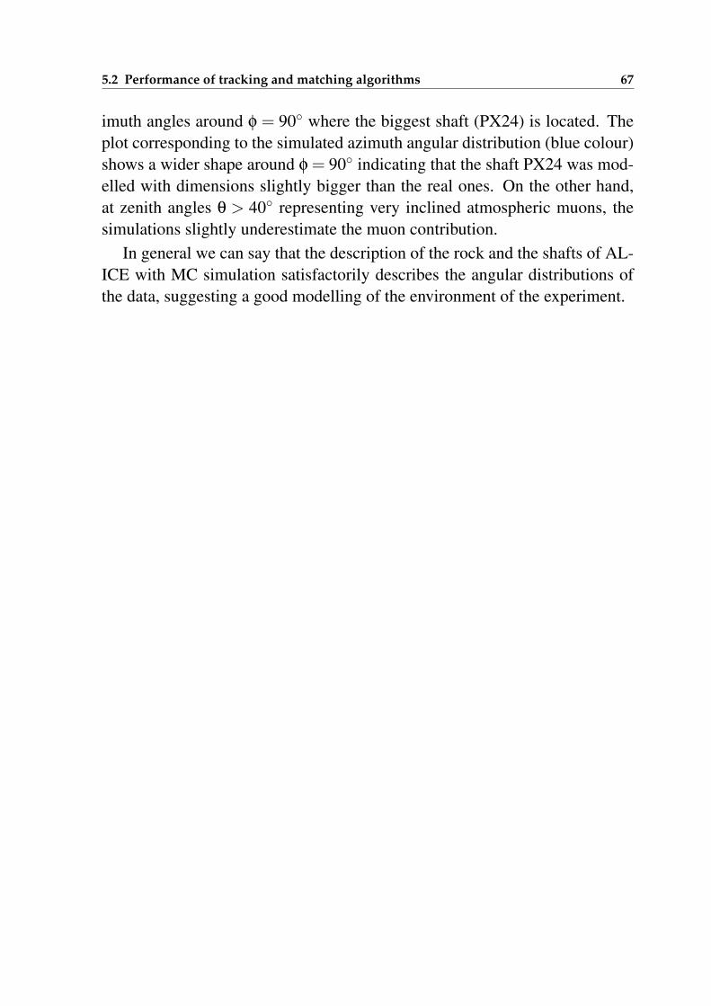
5.2 Performance of tracking and matching algorithms 67

imuth angles around φ = 90 where the biggest shaft (PX24) is located. Theplot corresponding to the simulated azimuth angular distribution (blue colour)shows a wider shape around φ = 90 indicating that the shaft PX24 was mod-elled with dimensions slightly bigger than the real ones. On the other hand,at zenith angles θ > 40 representing very inclined atmospheric muons, thesimulations slightly underestimate the muon contribution.

In general we can say that the description of the rock and the shafts of AL-ICE with MC simulation satisfactorily describes the angular distributions ofthe data, suggesting a good modelling of the environment of the experiment.

6Simulation strategy

6.1 Event generator and hadronic models

In order to explain the muon component detected by ALICE, a proper set ofmodern Monte Carlo tools is necessary to achieve a suitable EAS simulation.The simulation has to start with the first interaction of the primary cosmic raywith a nucleus of the upper atmosphere and subsequently describe all the EASdevelopment up to the ground level.

The Monte Carlo software CORSIKA1 [115], originally developed to per-form simulations for the KASCADE experiment [116], was adopted in thisthesis as event generator of primary cosmic rays. The CORSIKA code in-corporates different hadronic interaction models to simulate interactions anddecays of nuclei, hadrons, muons, electrons and photons in the atmosphere upto energies of about 1020 eV. In this work, two of the more recent CORSIKAversions where used: 6.990 [117] and 7.350 [118]. The main differences re-side in the implemented hadronic interaction models with their specific the-oretical formalisms and cross-sections data used to describe hadron-air andnucleus-air interactions in EAS.

The main hadronic interaction models included in CORSIKA are DPM-JET2 [119] used to describe interactions involving nuclei through the two-component Dual Parton Model, –EPOS3 [120] which introduces improve-ments concerning hard interactions as well as nuclear and high density effect,–NEXUS4 [121] which extrapolates up to higher energies features of VENUSand QGSJET in a parton model approach for initial stages of nuclear col-lisions in hadron-hadron interactions, –QGSJET5 [18, 19] which treats the

1 COsmic Ray SImulation for KAscade.2Dual Pcarton Model with JETs.3Energy conserving quantum mechanical multi-scattering approach, based on Partons Off-shell remnants

and Splitting parton ladders.4NEXt generation of Unified Scattering approach5Quark Gluon String model with JETs

69

70 Simulation strategy

hadronization process in the quark gluon string model and describes highenergy hadronic interactions using quasi-eikonal Pomeron6 parameterizationfor the elastic hadron-nucleon scattering amplitude, –SIBYLL [122] which isbased on the QCD mini-jet model to simulate hadronic interactions at extremehigh energies, and –VENUS7 [123] for ultra-relativistic heavy ion collisions.

All high-energy interaction models mentioned above were developed on asemihard Pome- ron approach, with the exception of SIBYLL which workson a mini-jet scheme. Both approaches are identical in what concerns highpT hadron production. However, the semihard Pomeron treatment providesan additional contribution, from the low virtuality domain (

∣∣q2∣∣ ' p2

T < Q20),

to secondary particle production and significantly enhances the predicted in-elasticity of hadronic interactions. Actually, in shower simulations is veryimportant the treatment of the transition region between central and peripheralcollisions, in particular when the average parton densities grow with the de-creasing impact parameter but keeping impact parameters large enough suchthat no density saturation is reached. In this scenario both, soft and semihardprocesses, are important to the same extent and give a notable contribution tothe interaction characteristics relevant for EAS physics.

In the latest versions of CORSIKA (7.3xx) there are two models includingthe early LHC data, for the first time, to constraint model parameters: EPOSLHC (v3400) and QGSJET II-04 [19].

In this work we have settle on QGSJET [18, 19] as the model for simu-lating the generation and development of the EAS. In order to test differentversions of the model, we have chosen QGSJET II-03 [18] implemented inCORSIKA version 6.990, and QGSJET II-04 [19] implemented in CORSIKAversion 7.350. Both models have, per se, a much more advanced description ofthe underlying physics with respect to the original QGSJET(01). All versionsof QGSJET are developed as Monte Carlo performances of the Quark GluonString [124] model, which was being generalized to treat nucleus-nucleus col-lisions and to describe the fragmentation of the nuclear spectator. All of thiswas done in the framework of the Reggeon Field Theory applying the semi-hard Pomeron approach (see [125] and references therein). The phenomeno-logical treatment of semihard processes in QGSJET gives rise to hadron jets

6 Pomeron is a Regge trajectory, a family of particles (composite objects) characterized by vacuum quantumnumbers, that could lead to logarithmically rising cross sections of hadronic collisions at high energies.

7Very Energetic Nuclear Scattering

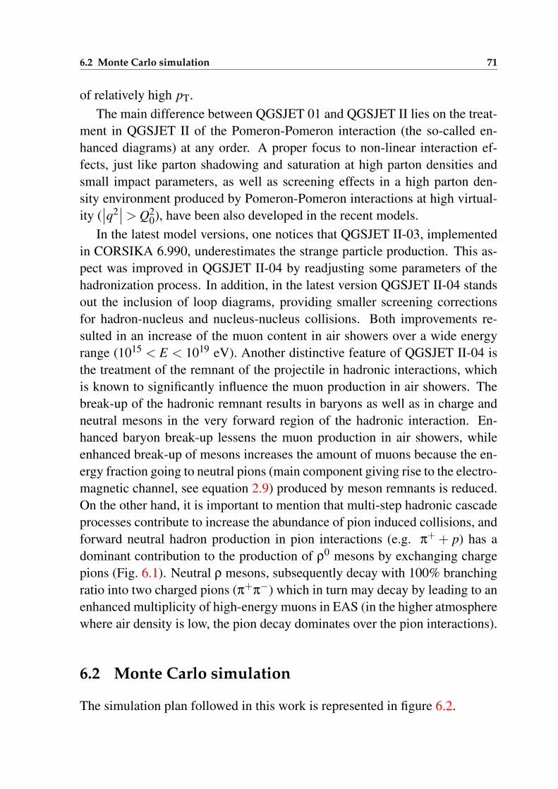
6.2 Monte Carlo simulation 71

of relatively high pT.The main difference between QGSJET 01 and QGSJET II lies on the treat-

ment in QGSJET II of the Pomeron-Pomeron interaction (the so-called en-hanced diagrams) at any order. A proper focus to non-linear interaction ef-fects, just like parton shadowing and saturation at high parton densities andsmall impact parameters, as well as screening effects in a high parton den-sity environment produced by Pomeron-Pomeron interactions at high virtual-ity (

∣∣q2∣∣> Q2

0), have been also developed in the recent models.In the latest model versions, one notices that QGSJET II-03, implemented

in CORSIKA 6.990, underestimates the strange particle production. This as-pect was improved in QGSJET II-04 by readjusting some parameters of thehadronization process. In addition, in the latest version QGSJET II-04 standsout the inclusion of loop diagrams, providing smaller screening correctionsfor hadron-nucleus and nucleus-nucleus collisions. Both improvements re-sulted in an increase of the muon content in air showers over a wide energyrange (1015 < E < 1019 eV). Another distinctive feature of QGSJET II-04 isthe treatment of the remnant of the projectile in hadronic interactions, whichis known to significantly influence the muon production in air showers. Thebreak-up of the hadronic remnant results in baryons as well as in charge andneutral mesons in the very forward region of the hadronic interaction. En-hanced baryon break-up lessens the muon production in air showers, whileenhanced break-up of mesons increases the amount of muons because the en-ergy fraction going to neutral pions (main component giving rise to the electro-magnetic channel, see equation 2.9) produced by meson remnants is reduced.On the other hand, it is important to mention that multi-step hadronic cascadeprocesses contribute to increase the abundance of pion induced collisions, andforward neutral hadron production in pion interactions (e.g. π++ p) has adominant contribution to the production of ρ0 mesons by exchanging chargepions (Fig. 6.1). Neutral ρ mesons, subsequently decay with 100% branchingratio into two charged pions (π+π−) which in turn may decay by leading to anenhanced multiplicity of high-energy muons in EAS (in the higher atmospherewhere air density is low, the pion decay dominates over the pion interactions).

6.2 Monte Carlo simulation

The simulation plan followed in this work is represented in figure 6.2.

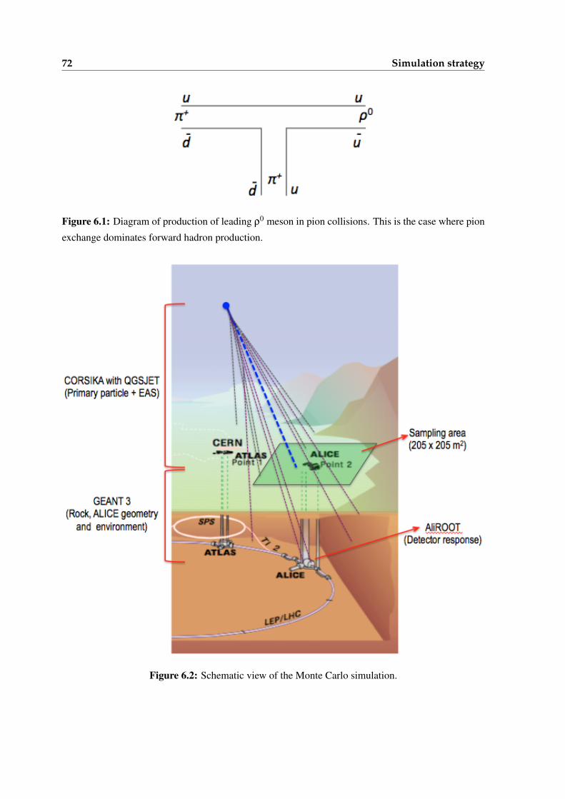
72 Simulation strategy

Figure 6.1: Diagram of production of leading ρ0 meson in pion collisions. This is the case where pion

exchange dominates forward hadron production.

Figure 6.2: Schematic view of the Monte Carlo simulation.

6.2 Monte Carlo simulation 73

The main steps of the simulation scheme consist of defining the primaryparticle giving rise to the EAS, performing the shower development throughthe atmosphere until the observation level, following the propagation of themuons through the rock and the environment around ALICE, as well as simu-lating the ALICE detector. All muons crossing the TPC active area are treatedby a detector response simulation that produces pseudo-raw data which arethen processed with the same reconstruction code that is applied to the realdata, including the TPC tracking algorithm and the track matching algorithm(Section 5.1) developed for this study.

The sampling area, that is the area at surface level in which the core ofthe shower (centre of the shower) is randomly scattered, has to be optimised.Actually, a too large area gives a fraction of simulated showers in which nomuon crosses the TPC of ALICE to the detriment of the simulation efficiency.On the contrary, a too small sampling area can lose events in which somemuons would fall inside the TPC, artificially decreasing the number of events,especially at low multiplicities. For this reason, the core of the shower wasrandomly scattered at ground level over an area covering 205 × 205 m2 cen-tered upon the nominal LCH beam crossing point corresponding to the ALICEexperiment (see figure 6.2). The optimisation of the size of this sampling areawas obtained with preliminary simulations. It was found that, when the corewas located outside this area, only a very small number of events gave riseto muons crossing the TPC and these events were only of low multiplicity(Nµ < 4). This sampling area contributes to minimize the number of generatedevents without creating any bias on the final results.

Two main methods were used to perform the simulations: simplified MonteCarlo (Section 6.2.2) and full Monte Carlo (Section 6.2.3).

In order to generate a shower it is important to define some initializationparameters. This is summarised in section 6.2.1.

6.2.1 CORSIKA initializations

Some of the most important parameters initialized in every CORSIKA run tosimulate the showers are:

• primary particle identification;

• energy range of primary particles;

74 Simulation strategy

• slope of differential primary energy spectrum;

• range of zenith angle;

• range of azimuth angle;

• the observation level;

• Earth’s magnetic field at the experiment location;

In our simulations we have chosen pure proton and pure iron as primarycosmic particles in order to have the lower and higher limits of mass compo-sitions.

Primaries in a wide energy range were generated, starting from 1012 eV upto 1018 eV. Simulations were run for small energy intervals within the wholerange in order to make more efficient the computing time, and in turn to coverthe energy range of primary cosmic rays giving rise to muons that can bedetected in ALICE.

The zenith angle range was limited to 0≤ θ≤ 50 while the azimuth anglerange was taken in the whole interval 0 ≤ φ≤ 360.

For all generated showers the starting altitude in the atmosphere was set to0 g/cm2 mass overburden.

The ground surface was selected as the observation level of the generatedshowers, which is 479 m above the sea level for the CERN Point 2 surfacelocation.

The first interaction point of hadronic primaries was defined with a randombehaviour according to the appropriate mean free path.

We assumed the default atmospheric model adopted by CORSIKA, whichis the U.S. standard atmosphere parameterized according to J. Linsley. The pa-rameters of this model can be found in [117]. The atmosphere density depen-dence with the altitude was modelled by dividing the atmosphere in 5 layers(i.e. 0 - 4, 4 - 10, 10 - 40, 40 - 100 and > 100 Km). The following expressionsreflect the dependence of the atmosphere density (T ) with the altitude (h), withparameters ai, bi and ci.

T (h) = ai +bi · e−h/ci i = 1, ...,4. (6.1)T (h) = ai−bi ·−h/ci i = 5. (6.2)

In the lower four layers the density decreases exponentially with the altitude(Eq. 6.1), while the fifth layer is characterized by a linear decreasing of density

6.2 Monte Carlo simulation 75

with the altitude (Eq. 6.2) until it finally vanishes. Based on the U.S. standardatmosphere, the parameter a5 = 0 in Eq. 6.2.

The Earth’s magnetic field was defined in correspondence to the geograph-ical location of the CERN. In this case magnetic field horizontal componentwas set to Bx = 22.1 µTesla whereas vertical component was set to Bz = 41.6µTesla. In CORSIKA, the component By = 0, by definition8.

The number of simulated showers is a decisive parameter during the simu-lation process since it allows to fix the time in a direct equivalence to the ex-perimental effective time. This allows an accurate comparison between mea-surements and simulations without any normalisation. The number of eventsfor a given energy interval depends on the flux, the solid angle, the area wherethe shower central axis is sampled and the measurement time, as follows,

Nev(E1,E2) = Φ×Ω×A×T (6.3)

In Eq. 6.3, the primary particle flux is given by Φ (m2 s sr TeV)−1, while Ω

(sr) is the solid angle, A (m2) is the sampling area and T (s) is the measure-ment time. The total (all-particle) flux Φ of primary particles was calculatedaccording to the poly-gonato model [47] which is explained in section 2.2. Itsvalue was estimated to be Φ(1TeV) = 0.225 ± 0.005 (m2 s sr TeV)−1. Thus,the energy dependence of the flux can be expressed as,

Φ(E1,E2) = 0.225∫ E2

E1

[E(TeV )

1(TeV )

]−γ

dE (6.4)

The exponent γ is the spectral index, defining the slope of the differential pri-mary energy spectrum. This value was set to γ = 2.7 for energies below theknee (Ek = 3×1015 eV) and γk = 3.0 for energies above the knee.

The QGSJET model was chosen to describe the high-energy hadronic in-teractions, as well as the cross sections derived from it. The differences inrapidity distribution between π0 and π± were taken into account according tothe LHC data. A realistic nuclear fragmentation depending on the transversemomenta was defined. The NKG formula [67] was enabled in order to cal-culate the electromagnetic subcascades analytically. The radius of the lateralNKG distribution was defined between 100 cm and 200 m, while the NKGlongitudinal development is sampled in vertical steps of 20 g/cm2. The valuesof low cutoff kinetic energies were chosen as Eh = 1 GeV, Eπ0 = 3 MeV, Eµ =

8 The reference system of CORSIKA is different from the ALICE coordinate system.

76 Simulation strategy

1 GeV, Eγ = 3 MeV, Ee− = 3 MeV, for hadrons (not including π0), π0, muons,photons and electrons respectively. The calculation of the muon multiple scat-tering angles followed the Moliere theory for large steps and were treated assingle Coulomb scattering events for small steps (see explanation in 2.3).

6.2.2 Simplified Monte Carlo procedure

Our simulations, mainly aimed to the study of the muon multiplicity distri-bution in ALICE, started with a simplified Monte Carlo procedure. This is afast and flexible method of estimating important parameters and observablesinvolved in the analysis before using a full simulation.

With the simplified Monte Carlo the muon transport through the rock abovethe ALICE hall is not explicitly modelled. Instead, to make the simulationfaster, the trajectory of the muons arriving at the surface level were extrap-olated as straight lines to the depth of ALICE. An energy cut value of Eµ =

16 GeV/cos(θ), where θ is the zenith angle of the muon, is imposed thusreflecting the effect of the rock. All muons passing this cut and crossing anarea of 17 m2, corresponding to the horizontal cross-sectional area of the TPC,with the centre located underground in correspondence with the centre of theTPC, are considered detected.

6.2.3 Full Monte Carlo procedure

The full simulation takes into account all possible interactions in matter sur-rounding the experiment. In each event, all muons crossing the ground levelare extrapolated to the horizontal mid-plane of the ALICE apparatus and flaggedif they hit an enlarged area of 36 m2 centred upon the TPC with no restrictionon the energy of the muons. Then, the position and momentum of all flaggedmuons, at ground level, are recorded and used as input to the AliRoot code [1].This is the ALICE framework where the ALICE experimental hall and the en-vironment above and around the apparatus as well as all the detectors are ac-curately described. Flagged muons are propagated through this environmentwith GEANT3 [126]. Details about the simulated environment surroundingALICE were explained in Section 4.5.

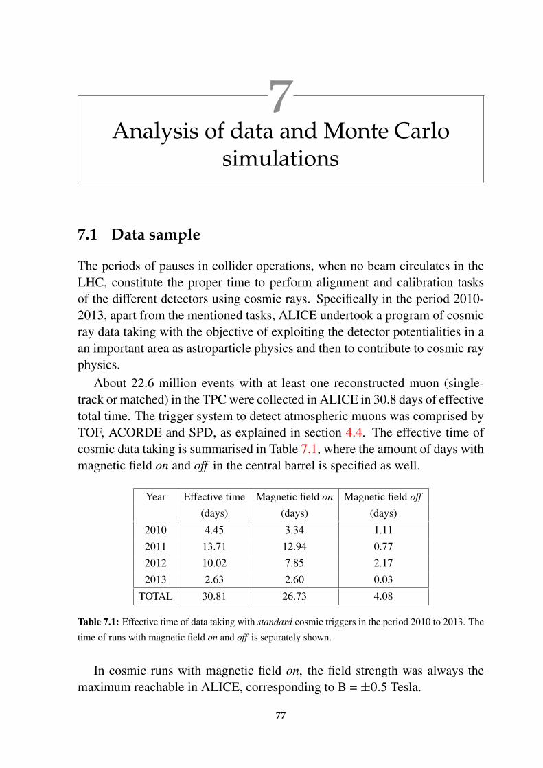
7Analysis of data and Monte Carlo

simulations

7.1 Data sample

The periods of pauses in collider operations, when no beam circulates in theLHC, constitute the proper time to perform alignment and calibration tasksof the different detectors using cosmic rays. Specifically in the period 2010-2013, apart from the mentioned tasks, ALICE undertook a program of cosmicray data taking with the objective of exploiting the detector potentialities in aan important area as astroparticle physics and then to contribute to cosmic rayphysics.

About 22.6 million events with at least one reconstructed muon (single-track or matched) in the TPC were collected in ALICE in 30.8 days of effectivetotal time. The trigger system to detect atmospheric muons was comprised byTOF, ACORDE and SPD, as explained in section 4.4. The effective time ofcosmic data taking is summarised in Table 7.1, where the amount of days withmagnetic field on and off in the central barrel is specified as well.

Year Effective time Magnetic field on Magnetic field off

(days) (days) (days)

2010 4.45 3.34 1.11

2011 13.71 12.94 0.77

2012 10.02 7.85 2.17

2013 2.63 2.60 0.03

TOTAL 30.81 26.73 4.08

Table 7.1: Effective time of data taking with standard cosmic triggers in the period 2010 to 2013. The

time of runs with magnetic field on and off is separately shown.

In cosmic runs with magnetic field on, the field strength was always themaximum reachable in ALICE, corresponding to B = ±0.5 Tesla.

77

78 Analysis of data and Monte Carlo simulations

The effective time was calculated run by run defining:

Effective time=Time of data taking×Detector live time×Reconstruction efficiency(7.1)

where,

Detector live time =L2aL0b

(7.2)

The time of data taking was the total time of a run from its start until itsstop. The detector live time was evaluated from the ratio L2a/L0b, where L0bgives the number of times a given detector is fired while L2a gives the numberof times the same trigger passes the CTP decision, the detector dead time andother vetoes, as explained in section 4.4.

The reconstruction efficiency, given by a number between 0 and 1, keepsinto account those events recorded but not reconstructed by the ALICE offlineframework.

The valid runs were required to satisfy, in every period of cosmic data tak-ing, the following selection criteria:

• run duration larger than 10 minutes;

• runs marked as “good run” by the Data Acquisition (DAQ) system andsuited for physics analysis;

• data acquired with a combination (logical OR) of at least two out of thethree trigger conditions (ACORDE, SPD and TOF) depending on the runperiod;

• TPC as readout detector;

The analysis of this thesis was centered on the multi-muon events, whichwe defined as those events with more than four reconstructed muons in theTPC (Nµ > 4). Finally, a sample of 7487 multi-muon events, was collectedout of a total of 22.6 million events which were detected in 30.8 days (interms of effective time).

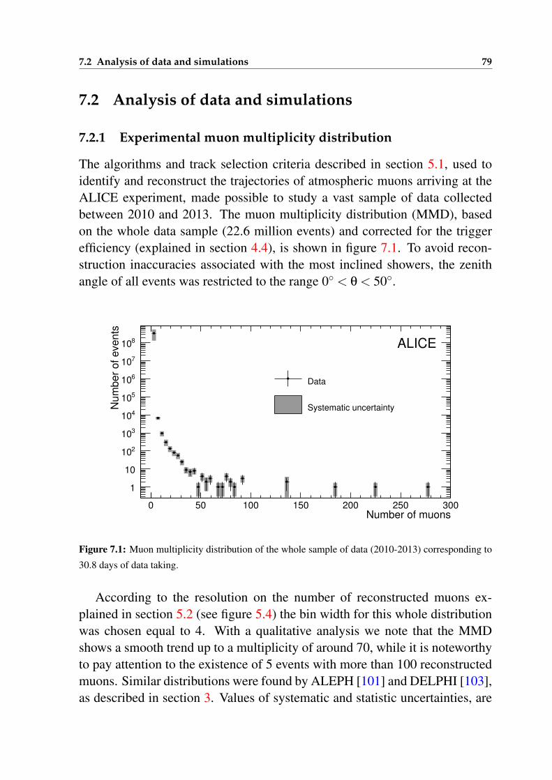
7.2 Analysis of data and simulations 79

7.2 Analysis of data and simulations

7.2.1 Experimental muon multiplicity distribution

The algorithms and track selection criteria described in section 5.1, used toidentify and reconstruct the trajectories of atmospheric muons arriving at theALICE experiment, made possible to study a vast sample of data collectedbetween 2010 and 2013. The muon multiplicity distribution (MMD), basedon the whole data sample (22.6 million events) and corrected for the triggerefficiency (explained in section 4.4), is shown in figure 7.1. To avoid recon-struction inaccuracies associated with the most inclined showers, the zenithangle of all events was restricted to the range 0 < θ < 50.

Number of muons0 50 100 150 200 250 300

Nu

mb

er

of

eve

nts

1

10

210

310

410

510

610

710

810 ALICE

Data

Systematic uncertainty

Figure 7.1: Muon multiplicity distribution of the whole sample of data (2010-2013) corresponding to

30.8 days of data taking.

According to the resolution on the number of reconstructed muons ex-plained in section 5.2 (see figure 5.4) the bin width for this whole distributionwas chosen equal to 4. With a qualitative analysis we note that the MMDshows a smooth trend up to a multiplicity of around 70, while it is noteworthyto pay attention to the existence of 5 events with more than 100 reconstructedmuons. Similar distributions were found by ALEPH [101] and DELPHI [103],as described in section 3. Values of systematic and statistic uncertainties, are

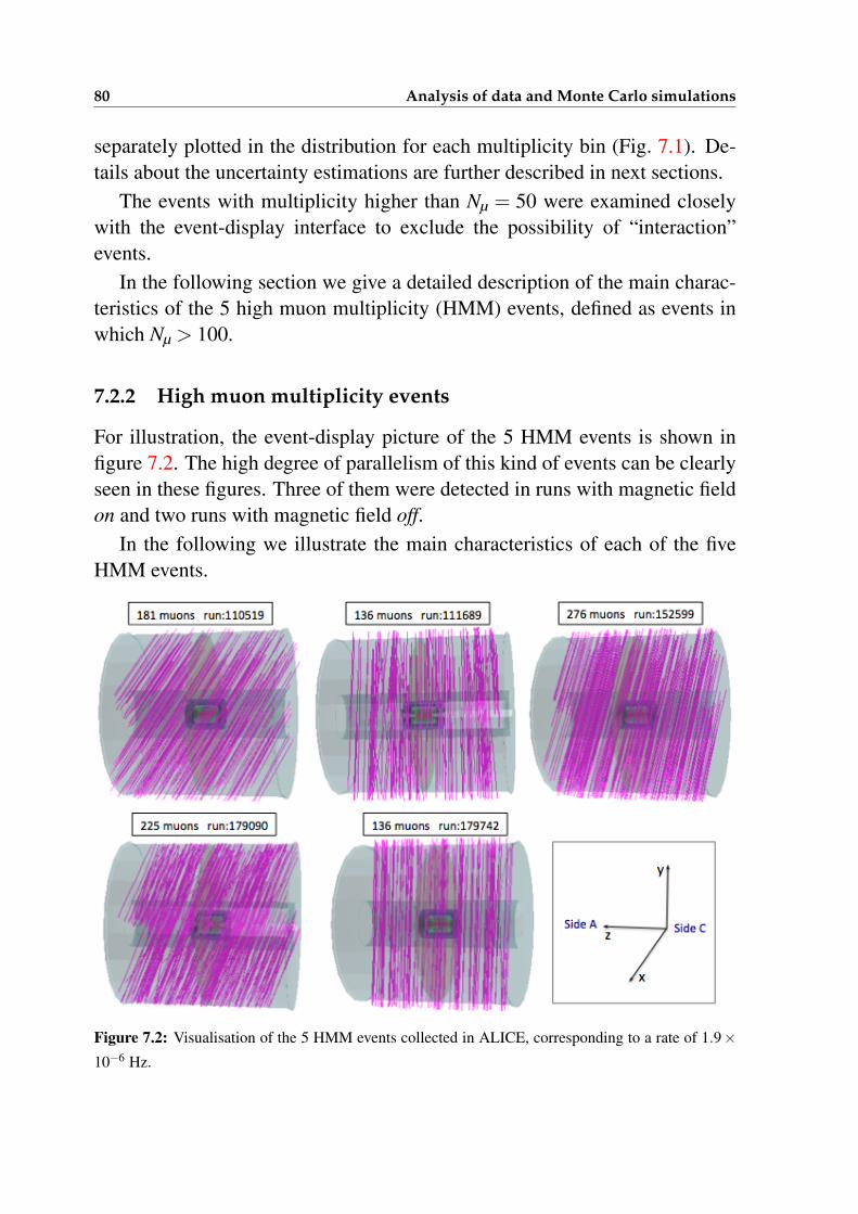
80 Analysis of data and Monte Carlo simulations

separately plotted in the distribution for each multiplicity bin (Fig. 7.1). De-tails about the uncertainty estimations are further described in next sections.

The events with multiplicity higher than Nµ = 50 were examined closelywith the event-display interface to exclude the possibility of “interaction”events.

In the following section we give a detailed description of the main charac-teristics of the 5 high muon multiplicity (HMM) events, defined as events inwhich Nµ > 100.

7.2.2 High muon multiplicity events

For illustration, the event-display picture of the 5 HMM events is shown infigure 7.2. The high degree of parallelism of this kind of events can be clearlyseen in these figures. Three of them were detected in runs with magnetic fieldon and two runs with magnetic field off.

In the following we illustrate the main characteristics of each of the fiveHMM events.

Figure 7.2: Visualisation of the 5 HMM events collected in ALICE, corresponding to a rate of 1.9×10−6 Hz.

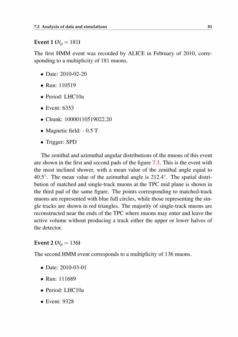
7.2 Analysis of data and simulations 81

Event 1 (Nµ = 181)

The first HMM event was recorded by ALICE in February of 2010, corre-sponding to a multiplicity of 181 muons.

• Date: 2010-02-20

• Run: 110519

• Period: LHC10a

• Event: 6353

• Chunk: 10000110519022.20

• Magnetic field: - 0.5 T

• Trigger: SPD

The zenithal and azimuthal angular distributions of the muons of this eventare shown in the first and second pads of the figure 7.3. This is the event withthe most inclined shower, with a mean value of the zenithal angle equal to40.5. The mean value of the azimuthal angle is 212.4. The spatial distri-bution of matched and single-track muons at the TPC mid plane is shown inthe third pad of the same figure. The points corresponding to matched-trackmuons are represented with blue full circles, while those representing the sin-gle tracks are shown in red triangles. The majority of single-track muons arereconstructed near the ends of the TPC where muons may enter and leave theactive volume without producing a track either the upper or lower halves ofthe detector.

Event 2 (Nµ = 136)

The second HMM event corresponds to a multiplicity of 136 muons.

• Date: 2010-03-01

• Run: 111689

• Period: LHC10a

• Event: 9328

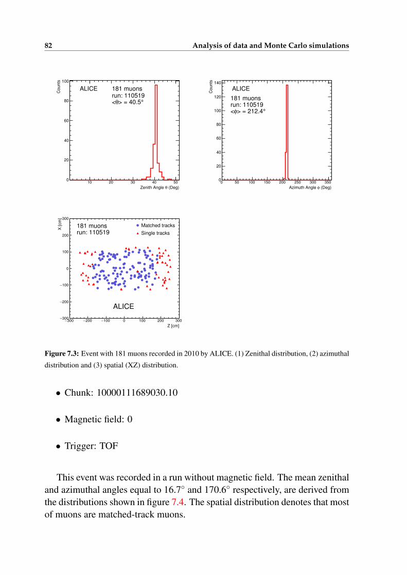
82 Analysis of data and Monte Carlo simulations

(Deg)θZenith Angle

10 20 30 40 50

Co

un

ts

0

20

40

60

80

100

ALICE 181 muonsrun: 110519

°> = 40.5θ<

(Deg)φAzimuth Angle

0 50 100 150 200 250 300 350

Co

un

ts

0

20

40

60

80

100

120

140

ALICE

181 muonsrun: 110519

°> = 212.4φ<

Z [cm]

300− 200− 100− 0 100 200 300

X [

cm

]

300−

200−

100−

0

100

200

300

Matched tracks

Single tracks

ALICE

181 muonsrun: 110519

Figure 7.3: Event with 181 muons recorded in 2010 by ALICE. (1) Zenithal distribution, (2) azimuthal

distribution and (3) spatial (XZ) distribution.

• Chunk: 10000111689030.10

• Magnetic field: 0

• Trigger: TOF

This event was recorded in a run without magnetic field. The mean zenithaland azimuthal angles equal to 16.7 and 170.6 respectively, are derived fromthe distributions shown in figure 7.4. The spatial distribution denotes that mostof muons are matched-track muons.

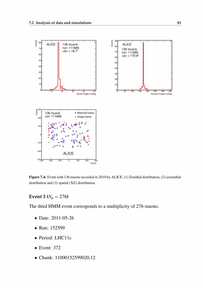
7.2 Analysis of data and simulations 83

(Deg)θZenith Angle

10 20 30 40 50

Co

un

ts

0

10

20

30

40

50

60

70

80ALICE 136 muons

run: 111689°> = 16.7θ<

(Deg)φAzimuth Angle

0 50 100 150 200 250 300 350

Co

un

ts

0

10

20

30

40

50

60

70

80

90

ALICE

136 muonsrun: 111689

°> = 170.6φ<

Z [cm]

300− 200− 100− 0 100 200 300

X [

cm

]

300−

200−

100−

0

100

200

300

Matched tracks

Single tracks

ALICE

136 muonsrun: 111689

Figure 7.4: Event with 136 muons recorded in 2010 by ALICE. (1) Zenithal distribution, (2) azimuthal

distribution and (3) spatial (XZ) distribution.

Event 3 (Nµ = 276)

The third HMM event corresponds to a multiplicity of 276 muons.

• Date: 2011-05-26

• Run: 152599

• Period: LHC11c

• Event: 372

• Chunk: 11000152599020.12

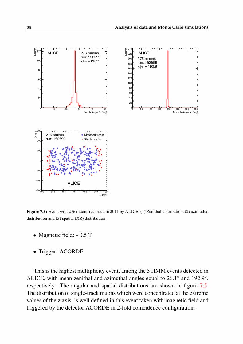
84 Analysis of data and Monte Carlo simulations

(Deg)θZenith Angle

10 20 30 40 50

Co

un

ts

0

20

40

60

80

100

120ALICE 276 muons

run: 152599°> = 26.1θ<

(Deg)φAzimuth Angle

0 50 100 150 200 250 300 350

Co

un

ts

0

20

40

60

80

100

120

140

160

180

200

220

240

ALICE

276 muonsrun: 152599

°> = 192.9φ<

Z [cm]

300− 200− 100− 0 100 200 300

X [

cm

]

300−

200−

100−

0

100

200

300

Matched tracks

Single tracks

ALICE

276 muonsrun: 152599

Figure 7.5: Event with 276 muons recorded in 2011 by ALICE. (1) Zenithal distribution, (2) azimuthal

distribution and (3) spatial (XZ) distribution.

• Magnetic field: - 0.5 T

• Trigger: ACORDE

This is the highest multiplicity event, among the 5 HMM events detected inALICE, with mean zenithal and azimuthal angles equal to 26.1 and 192.9,respectively. The angular and spatial distributions are shown in figure 7.5.The distribution of single-track muons which were concentrated at the extremevalues of the z axis, is well defined in this event taken with magnetic field andtriggered by the detector ACORDE in 2-fold coincidence configuration.

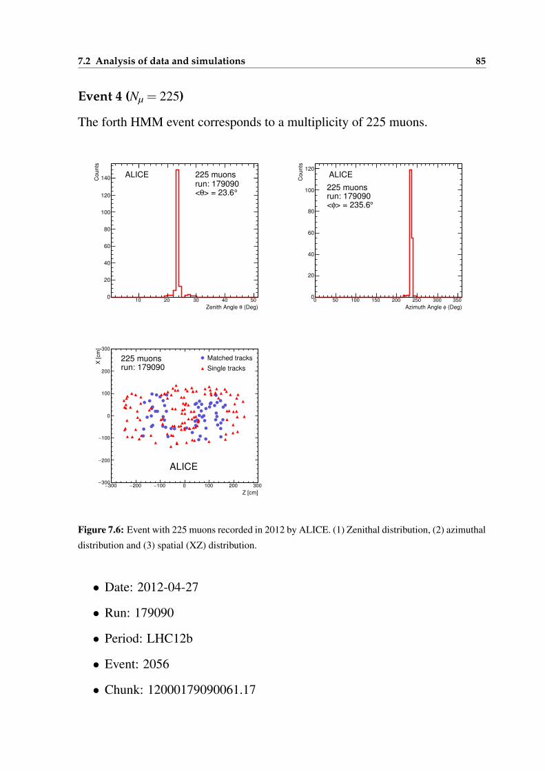
7.2 Analysis of data and simulations 85

Event 4 (Nµ = 225)

The forth HMM event corresponds to a multiplicity of 225 muons.

(Deg)θZenith Angle

10 20 30 40 50

Co

un

ts

0

20

40

60

80

100

120

140 ALICE 225 muonsrun: 179090

°> = 23.6θ<

(Deg)φAzimuth Angle

0 50 100 150 200 250 300 350C

ou

nts

0

20

40

60

80

100

120ALICE

225 muonsrun: 179090

°> = 235.6φ<

Z [cm]

300− 200− 100− 0 100 200 300

X [

cm

]

300−

200−

100−

0

100

200

300

Matched tracks

Single tracks

ALICE

225 muonsrun: 179090

Figure 7.6: Event with 225 muons recorded in 2012 by ALICE. (1) Zenithal distribution, (2) azimuthal

distribution and (3) spatial (XZ) distribution.

• Date: 2012-04-27

• Run: 179090

• Period: LHC12b

• Event: 2056

• Chunk: 12000179090061.17

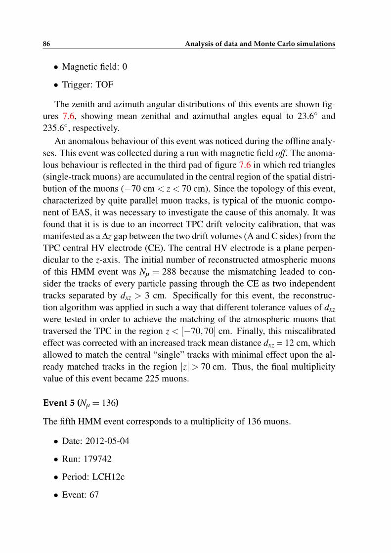
86 Analysis of data and Monte Carlo simulations

• Magnetic field: 0

• Trigger: TOF

The zenith and azimuth angular distributions of this events are shown fig-ures 7.6, showing mean zenithal and azimuthal angles equal to 23.6 and235.6, respectively.

An anomalous behaviour of this event was noticed during the offline analy-ses. This event was collected during a run with magnetic field off. The anoma-lous behaviour is reflected in the third pad of figure 7.6 in which red triangles(single-track muons) are accumulated in the central region of the spatial distri-bution of the muons (−70 cm < z < 70 cm). Since the topology of this event,characterized by quite parallel muon tracks, is typical of the muonic compo-nent of EAS, it was necessary to investigate the cause of this anomaly. It wasfound that it is is due to an incorrect TPC drift velocity calibration, that wasmanifested as a ∆z gap between the two drift volumes (A and C sides) from theTPC central HV electrode (CE). The central HV electrode is a plane perpen-dicular to the z-axis. The initial number of reconstructed atmospheric muonsof this HMM event was Nµ = 288 because the mismatching leaded to con-sider the tracks of every particle passing through the CE as two independenttracks separated by dxz > 3 cm. Specifically for this event, the reconstruc-tion algorithm was applied in such a way that different tolerance values of dxzwere tested in order to achieve the matching of the atmospheric muons thattraversed the TPC in the region z < [−70,70] cm. Finally, this miscalibratedeffect was corrected with an increased track mean distance dxz = 12 cm, whichallowed to match the central “single” tracks with minimal effect upon the al-ready matched tracks in the region |z|> 70 cm. Thus, the final multiplicityvalue of this event became 225 muons.

Event 5 (Nµ = 136)

The fifth HMM event corresponds to a multiplicity of 136 muons.

• Date: 2012-05-04

• Run: 179742

• Period: LCH12c

• Event: 67

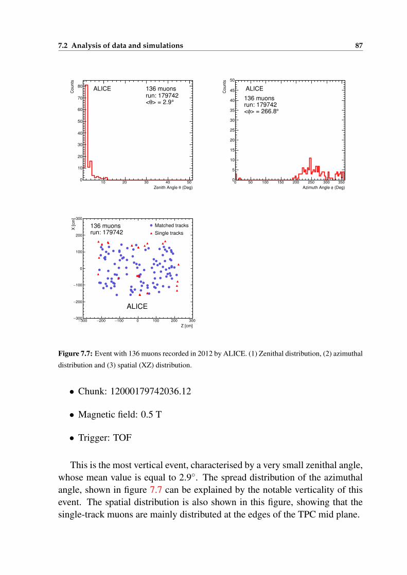
7.2 Analysis of data and simulations 87

(Deg)θZenith Angle

10 20 30 40 50

Co

un

ts

0

10

20

30

40

50

60

70

80ALICE 136 muons

run: 179742°> = 2.9θ<

(Deg)φAzimuth Angle

0 50 100 150 200 250 300 350

Co

un

ts

0

5

10

15

20

25

30

35

40

45

50

ALICE

136 muonsrun: 179742

°> = 266.8φ<

Z [cm]

300− 200− 100− 0 100 200 300

X [

cm

]

300−

200−

100−

0

100

200

300

Matched tracks

Single tracks

ALICE

136 muonsrun: 179742

Figure 7.7: Event with 136 muons recorded in 2012 by ALICE. (1) Zenithal distribution, (2) azimuthal

distribution and (3) spatial (XZ) distribution.

• Chunk: 12000179742036.12

• Magnetic field: 0.5 T

• Trigger: TOF

This is the most vertical event, characterised by a very small zenithal angle,whose mean value is equal to 2.9. The spread distribution of the azimuthalangle, shown in figure 7.7 can be explained by the notable verticality of thisevent. The spatial distribution is also shown in this figure, showing that thesingle-track muons are mainly distributed at the edges of the TPC mid plane.

88 Analysis of data and Monte Carlo simulations

The number of muons for each of the 5 HMM events is shown in table 7.2along with the corresponding run number, trigger and magnetic field, whilethe mean values of the zenith and azimuth angular distributions are in the nexttwo columns. The areal density is shown in the last column, assuming that thehorizontal cross-sectional area of the TPC is 17 m2, given z(m)=[−2.5,2.5]and x(m)=[−1.7,1.7] and keeping into account the direction of the shower.

Number Run Trigger B (T) < θ > < φ > Areal density

of muons (degrees) (degrees) (m−2)

181 110519 SPD -0.5 40.5 212.4 14.0

136 111689 TOF 0 16.7 170.9 8.4

276 152599 ACORDE -0.5 26.1 192.9 18.1

225 179090 TOF 0 23.6 235.6 14.4

136 179742 TOF 0.5 2.9 266.8 8.0

Table 7.2: The main characteristics of the 5 HMM events found in 30.8 days of data taking in the

ALICE detector.

The highest multiplicity event reconstructed in the TPC was found to con-tain 276 muons, which corresponds to a muon areal density of 18.1 m−2. The5 HMM events occurred with a frequency of 1.9×10−6 Hz.

Study of the TPC fiducial area

Most of muons are inside a fiducial area A = 17 m2, given by the limits−1.7 m < x < 1.7 m and−2.5 m < z < 2.5 m in the middle plane of the TPC.This is shown in figure 7.8 in which the spatial xz distribution of the muonsin the TPC mid plane is given. In addition, we must take into account thatthe areal density has an implied associated uncertainty related to the TPC ef-fective area. In order to report an accurate value of the event density with itsuncertainty, a TPC fiducial area value was estimated with its error.

Considering that the maximum accepted distance between every pair oftracks (up and down) in the horizontal mid plane of the TPC is 3 cm, we mightestimate the uncertainty of the axis coordinates (x,z) as 6 cm. Given this con-servative error value, the estimated fiducial area of the TPC due to its horizon-tal cylindrical geometry results 17±0.5 m2. In turn, the error on the numberof reconstructed muons, counting both matched and single-track muons, wasestimated as being around 5% for Nµ > 100. By knowing the uncertainties

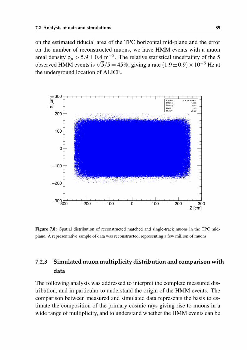
7.2 Analysis of data and simulations 89

on the estimated fiducial area of the TPC horizontal mid-plane and the erroron the number of reconstructed muons, we have HMM events with a muonareal density ρµ > 5.9± 0.4 m−2. The relative statistical uncertainty of the 5observed HMM events is

√5/5 = 45%, giving a rate (1.9±0.9)×10−6 Hz at

the underground location of ALICE.

Figure 7.8: Spatial distribution of reconstructed matched and single-track muons in the TPC mid-

plane. A representative sample of data was reconstructed, representing a few million of muons.

7.2.3 Simulated muon multiplicity distribution and comparison with

data

The following analysis was addressed to interpret the complete measured dis-tribution, and in particular to understand the origin of the HMM events. Thecomparison between measured and simulated data represents the basis to es-timate the composition of the primary cosmic rays giving rise to muons in awide range of multiplicity, and to understand whether the HMM events can be

90 Analysis of data and Monte Carlo simulations

described with standard hadronic models or whether they have to be explainedwith different production mechanisms.

Low-intermediate multiplicity

As a first step we tried to reproduce with MC simulation the MMD in thelow-intermediate multiplicity region.

At this purpose we followed the Monte Carlo simulation strategy previ-ously described in broad terms in chapter 6, to obtain the expected distribu-tion. For this first step was used CORSIKA 6.990 with QGSJET II-03 modelas hadronic interaction model, and a pure proton and pure iron (56Fe) samples.The proton sample provides a lower limit on the number of events for a givenmultiplicity, while the iron sample provides an upper limit.

The main interest of this research was the multi-muon events (Nµ > 4).Nevertheless, it is important to assure the understanding of the complete sam-ple of recorded data, including the low multiplicities. For this purpose, thesimplified Monte Carlo procedure (see description in section 6.2.2) was fol-lowed in order to generate primary cosmic rays with the two mentioned com-positions, with energies E > 1012 eV.

This preliminary assessment with the simplified Monte Carlo simulationproduced the following results:

• The single muon events are mostly produced by primary energies in therange 1012 < E < 1013 eV.

• Primary cosmic rays of either composition, pure proton or pure iron, inthe energy range 1012 < E < 1014 eV produce events with a multiplicityrange from 1≤ Nµ ≤ 4.

After these preliminary results, since our purpose is to study multi-muonevents, it was decided to simulate only events with primary energies E > 1014

eV, following both, simplified and full Monte Carlo procedures described inthe sections 6.2.2 and 6.2.3. All the events studied with the simplified MCmethod, were subsequently considered for a complete analysis using the fullsimulation which takes into account all possible interactions in the matter sur-rounding ALICE and the response of each detector.

Samples of proton and iron primary cosmic rays, were generated in therange of energy 1014 < E < 1018 eV. In this range the composition of primary

7.2 Analysis of data and simulations 91

particles is a mixture of many species of nuclei in a ratio not well-known andwhich varies with energy. Therefore, the analysis with a pure proton samplerepresents the light composition and a pure iron sample represents a composi-tion dominated by heavy nuclei. The zenith angle of generated showers wasrestricted to 0 < θ < 50. The typical power law energy spectrum, E−γ, wassimulated with the spectral index γ = 2.7± 0.03 for energies below the knee(Ek = 3×1015 eV) and γk = 3.0±0.03 for energies above the knee. The total(all-particle) flux Φ of primary particles was calculated according to the poly-gonato model [47] as explained in section 6.2.1. The primary particles weregenerated with the appropriate flux in the following energy intervals:

1014 < E < 1015 eV, 1015 < E < 3×1015 eV, 3×1015 < E < 1016 eV,

1016 < E < 3×1016 eV, 3×1016 < E < 1017 eV, 1017 < E < 3×1017 eV,

3×1017 < E < 1018 eV.

The simulation in separate energy intervals is very convenient to populateevery energy bin with the proper number of events. This procedure saves com-puting time by preventing a usually large and unnecessary amount of eventsin the first range of energy while populates the larger energy bins accordingly.The generated events were used four times (oversample = 4) only in the firstenergy interval while in the other intervals the events were used only once.

For the purpose of a straightforward comparison of the MMD data with theMonte Carlo expectation, the events were simulated corresponding to a timeequivalent to 30.8 days. Thus, there is not need to apply arbitrary normali-sation factors. In figure 7.9 the MMD simulated with both, proton and ironprimaries, was compared with the MMD obtained with the data. For easy ofcomparison, the values of the simulated distributions were fitted with power-law functions to obtain the trend of the multiplicity for proton and iron sample.

From this figure we find that at lower multiplicities, Nµ < 20, correspondingto lower primary energies, the data approach the proton curve, which repre-sents a light ion composition of the primary cosmic ray flux, while at highermultiplicity (20 < Nµ < 30) data lie closer to the iron curve, representing aheavier composition. This trend suggests that the average mass of the pri-maries become heavier with the increasing energy, a result consistent withseveral previous experiments [5, 40, 93]. At higher multiplicity (Nµ > 30), thelow statistics (less than 10 events per point) does not allow any conclusion on

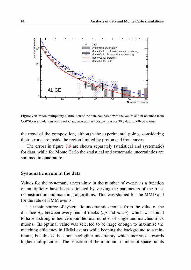
92 Analysis of data and Monte Carlo simulations

Number of muons10 20 30 40 50 60 70

Num

ber

of events

1

10

210

310

ALICE

Data

Systematic uncertainty

Monte Carlo: proton as primary cosmic ray

Monte Carlo: Fe as primary cosmic ray

Monte Carlo: proton fit

Monte Carlo: Fe fit

Figure 7.9: Muon multiplicity distribution of the data compared with the values and fit obtained from

CORSIKA simulations with proton and iron primary cosmic rays for 30.8 days of effective time.

the trend of the composition, although the experimental points, consideringtheir errors, are inside the region limited by proton and iron curves.

The errors in figure 7.9 are shown separately (statistical and systematic)for data, while for Monte Carlo the statistical and systematic uncertainties aresummed in quadrature.

Systematic errors in the data

Values for the systematic uncertainty in the number of events as a functionof multiplicity have been estimated by varying the parameters of the trackreconstruction and matching algorithms. This was studied for the MMD andfor the rate of HMM events.

The main source of systematic uncertainties comes from the value of thedistance dxz between every pair of tracks (up and down), which was foundto have a strong influence upon the final number of single and matched trackmuons. Its optimal value was selected to be large enough to maximise thematching efficiency in HMM events while keeping the background to a min-imum, but this adds a non negligible uncertainty which increases towardshigher multiplicities. The selection of the minimum number of space points

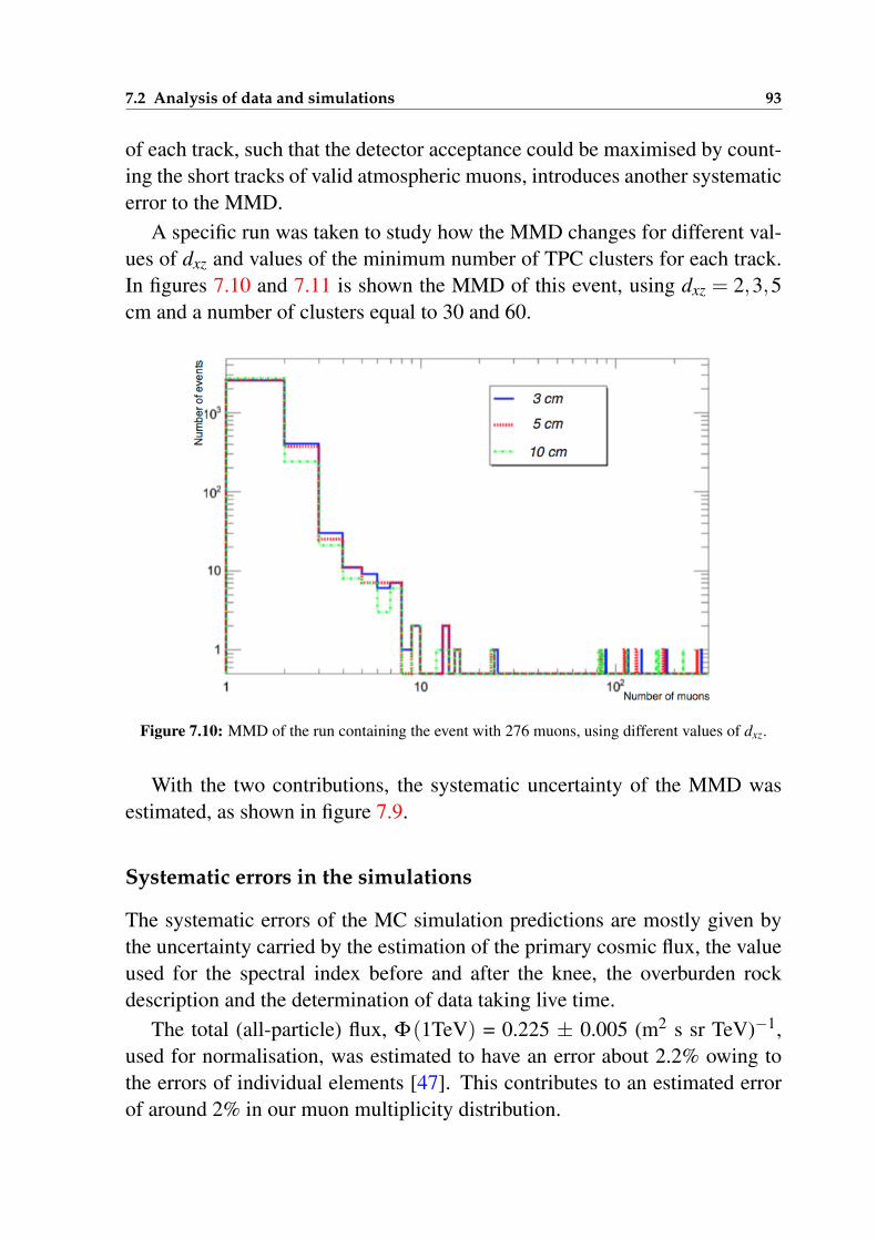
7.2 Analysis of data and simulations 93

of each track, such that the detector acceptance could be maximised by count-ing the short tracks of valid atmospheric muons, introduces another systematicerror to the MMD.

A specific run was taken to study how the MMD changes for different val-ues of dxz and values of the minimum number of TPC clusters for each track.In figures 7.10 and 7.11 is shown the MMD of this event, using dxz = 2,3,5cm and a number of clusters equal to 30 and 60.

Figure 7.10: MMD of the run containing the event with 276 muons, using different values of dxz.

With the two contributions, the systematic uncertainty of the MMD wasestimated, as shown in figure 7.9.

Systematic errors in the simulations

The systematic errors of the MC simulation predictions are mostly given bythe uncertainty carried by the estimation of the primary cosmic flux, the valueused for the spectral index before and after the knee, the overburden rockdescription and the determination of data taking live time.

The total (all-particle) flux, Φ(1TeV) = 0.225 ± 0.005 (m2 s sr TeV)−1,used for normalisation, was estimated to have an error about 2.2% owing tothe errors of individual elements [47]. This contributes to an estimated errorof around 2% in our muon multiplicity distribution.

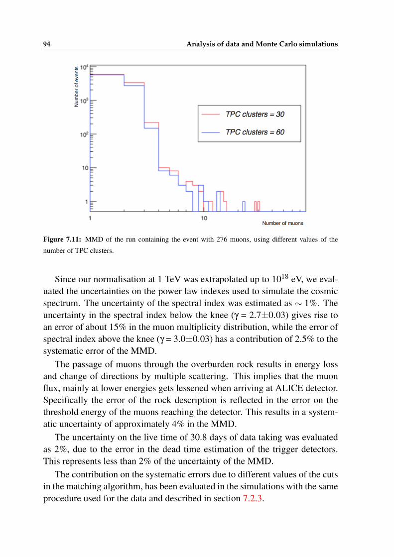
94 Analysis of data and Monte Carlo simulations

Figure 7.11: MMD of the run containing the event with 276 muons, using different values of the

number of TPC clusters.

Since our normalisation at 1 TeV was extrapolated up to 1018 eV, we eval-uated the uncertainties on the power law indexes used to simulate the cosmicspectrum. The uncertainty of the spectral index was estimated as ∼ 1%. Theuncertainty in the spectral index below the knee (γ = 2.7±0.03) gives rise toan error of about 15% in the muon multiplicity distribution, while the error ofspectral index above the knee (γ = 3.0±0.03) has a contribution of 2.5% to thesystematic error of the MMD.

The passage of muons through the overburden rock results in energy lossand change of directions by multiple scattering. This implies that the muonflux, mainly at lower energies gets lessened when arriving at ALICE detector.Specifically the error of the rock description is reflected in the error on thethreshold energy of the muons reaching the detector. This results in a system-atic uncertainty of approximately 4% in the MMD.

The uncertainty on the live time of 30.8 days of data taking was evaluatedas 2%, due to the error in the dead time estimation of the trigger detectors.This represents less than 2% of the uncertainty of the MMD.

The contribution on the systematic errors due to different values of the cutsin the matching algorithm, has been evaluated in the simulations with the sameprocedure used for the data and described in section 7.2.3.

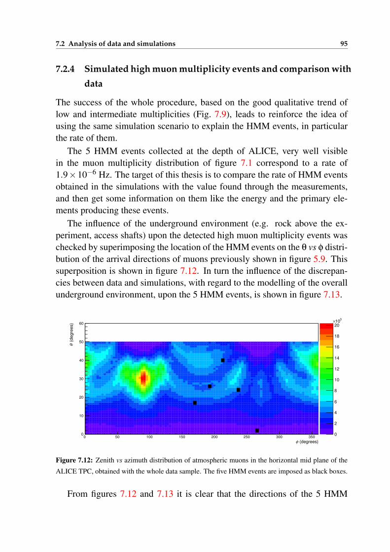
7.2 Analysis of data and simulations 95

7.2.4 Simulated high muon multiplicity events and comparison with

data

The success of the whole procedure, based on the good qualitative trend oflow and intermediate multiplicities (Fig. 7.9), leads to reinforce the idea ofusing the same simulation scenario to explain the HMM events, in particularthe rate of them.

The 5 HMM events collected at the depth of ALICE, very well visiblein the muon multiplicity distribution of figure 7.1 correspond to a rate of1.9×10−6 Hz. The target of this thesis is to compare the rate of HMM eventsobtained in the simulations with the value found through the measurements,and then get some information on them like the energy and the primary ele-ments producing these events.

The influence of the underground environment (e.g. rock above the ex-periment, access shafts) upon the detected high muon multiplicity events waschecked by superimposing the location of the HMM events on the θ vs φ distri-bution of the arrival directions of muons previously shown in figure 5.9. Thissuperposition is shown in figure 7.12. In turn the influence of the discrepan-cies between data and simulations, with regard to the modelling of the overallunderground environment, upon the 5 HMM events, is shown in figure 7.13.

(degrees)φ0 50 100 150 200 250 300 350

(d

eg

ree

s)

θ

0

10

20

30

40

50

60

0

2

4

6

8

10

12

14

16

18

20

310×

Figure 7.12: Zenith vs azimuth distribution of atmospheric muons in the horizontal mid plane of the

ALICE TPC, obtained with the whole data sample. The five HMM events are imposed as black boxes.

From figures 7.12 and 7.13 it is clear that the directions of the 5 HMM

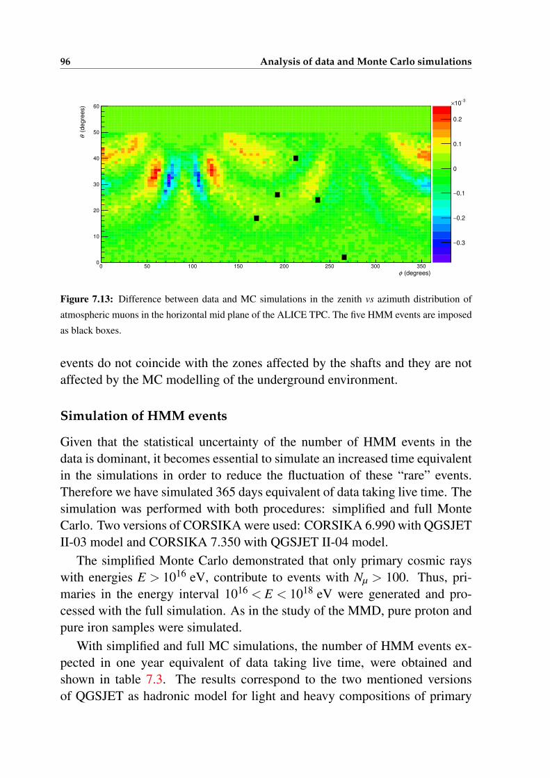
96 Analysis of data and Monte Carlo simulations

(degrees)φ0 50 100 150 200 250 300 350

(d

eg

ree

s)

θ

0

10

20

30

40

50

60

0.3−

0.2−

0.1−

0

0.1

0.2

3−10×

Figure 7.13: Difference between data and MC simulations in the zenith vs azimuth distribution of

atmospheric muons in the horizontal mid plane of the ALICE TPC. The five HMM events are imposed

as black boxes.

events do not coincide with the zones affected by the shafts and they are notaffected by the MC modelling of the underground environment.

Simulation of HMM events

Given that the statistical uncertainty of the number of HMM events in thedata is dominant, it becomes essential to simulate an increased time equivalentin the simulations in order to reduce the fluctuation of these “rare” events.Therefore we have simulated 365 days equivalent of data taking live time. Thesimulation was performed with both procedures: simplified and full MonteCarlo. Two versions of CORSIKA were used: CORSIKA 6.990 with QGSJETII-03 model and CORSIKA 7.350 with QGSJET II-04 model.

The simplified Monte Carlo demonstrated that only primary cosmic rayswith energies E > 1016 eV, contribute to events with Nµ > 100. Thus, pri-maries in the energy interval 1016 < E < 1018 eV were generated and pro-cessed with the full simulation. As in the study of the MMD, pure proton andpure iron samples were simulated.

With simplified and full MC simulations, the number of HMM events ex-pected in one year equivalent of data taking live time, were obtained andshown in table 7.3. The results correspond to the two mentioned versionsof QGSJET as hadronic model for light and heavy compositions of primary

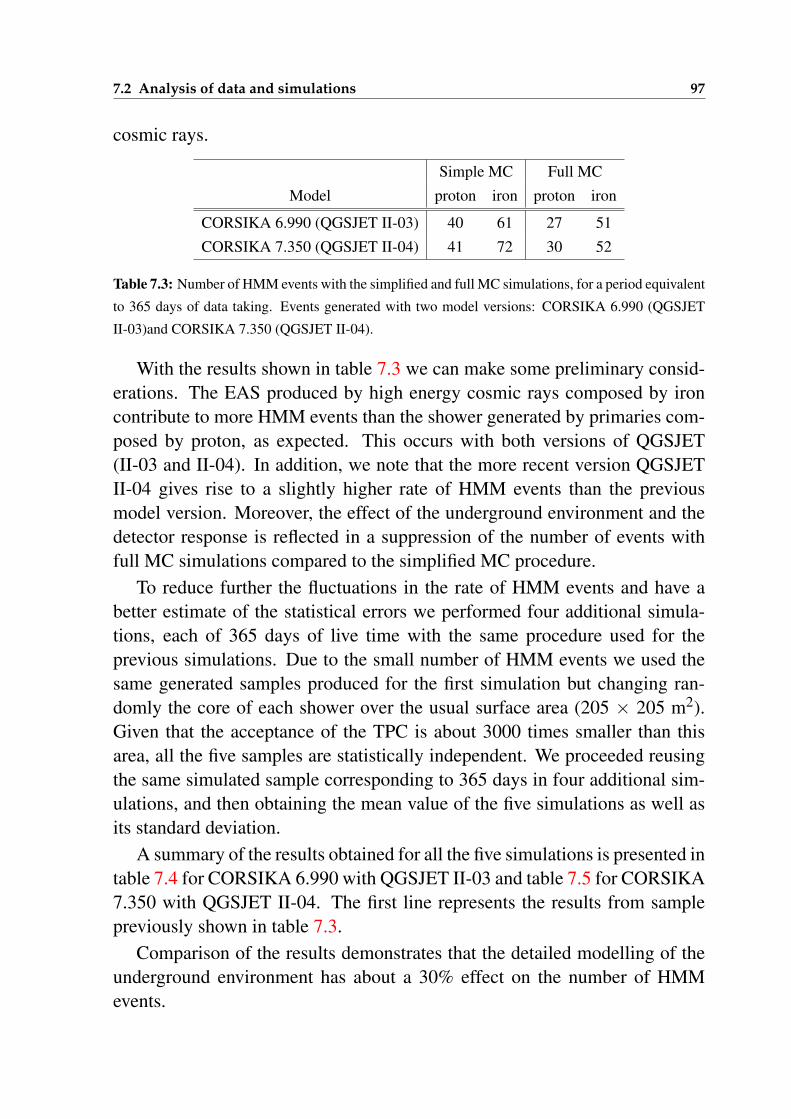
7.2 Analysis of data and simulations 97

cosmic rays.

Simple MC Full MC

Model proton iron proton iron

CORSIKA 6.990 (QGSJET II-03) 40 61 27 51

CORSIKA 7.350 (QGSJET II-04) 41 72 30 52

Table 7.3: Number of HMM events with the simplified and full MC simulations, for a period equivalent

to 365 days of data taking. Events generated with two model versions: CORSIKA 6.990 (QGSJET

II-03)and CORSIKA 7.350 (QGSJET II-04).

With the results shown in table 7.3 we can make some preliminary consid-erations. The EAS produced by high energy cosmic rays composed by ironcontribute to more HMM events than the shower generated by primaries com-posed by proton, as expected. This occurs with both versions of QGSJET(II-03 and II-04). In addition, we note that the more recent version QGSJETII-04 gives rise to a slightly higher rate of HMM events than the previousmodel version. Moreover, the effect of the underground environment and thedetector response is reflected in a suppression of the number of events withfull MC simulations compared to the simplified MC procedure.

To reduce further the fluctuations in the rate of HMM events and have abetter estimate of the statistical errors we performed four additional simula-tions, each of 365 days of live time with the same procedure used for theprevious simulations. Due to the small number of HMM events we used thesame generated samples produced for the first simulation but changing ran-domly the core of each shower over the usual surface area (205 × 205 m2).Given that the acceptance of the TPC is about 3000 times smaller than thisarea, all the five samples are statistically independent. We proceeded reusingthe same simulated sample corresponding to 365 days in four additional sim-ulations, and then obtaining the mean value of the five simulations as well asits standard deviation.

A summary of the results obtained for all the five simulations is presented intable 7.4 for CORSIKA 6.990 with QGSJET II-03 and table 7.5 for CORSIKA7.350 with QGSJET II-04. The first line represents the results from samplepreviously shown in table 7.3.

Comparison of the results demonstrates that the detailed modelling of theunderground environment has about a 30% effect on the number of HMMevents.

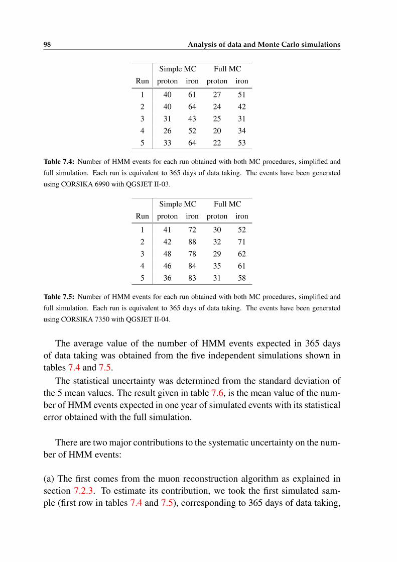
98 Analysis of data and Monte Carlo simulations

Simple MC Full MC

Run proton iron proton iron

1 40 61 27 51

2 40 64 24 42

3 31 43 25 31

4 26 52 20 34

5 33 64 22 53

Table 7.4: Number of HMM events for each run obtained with both MC procedures, simplified and

full simulation. Each run is equivalent to 365 days of data taking. The events have been generated

using CORSIKA 6990 with QGSJET II-03.

Simple MC Full MC

Run proton iron proton iron

1 41 72 30 52

2 42 88 32 71

3 48 78 29 62

4 46 84 35 61

5 36 83 31 58

Table 7.5: Number of HMM events for each run obtained with both MC procedures, simplified and

full simulation. Each run is equivalent to 365 days of data taking. The events have been generated

using CORSIKA 7350 with QGSJET II-04.

The average value of the number of HMM events expected in 365 daysof data taking was obtained from the five independent simulations shown intables 7.4 and 7.5.

The statistical uncertainty was determined from the standard deviation ofthe 5 mean values. The result given in table 7.6, is the mean value of the num-ber of HMM events expected in one year of simulated events with its statisticalerror obtained with the full simulation.

There are two major contributions to the systematic uncertainty on the num-ber of HMM events:

(a) The first comes from the muon reconstruction algorithm as explained insection 7.2.3. To estimate its contribution, we took the first simulated sam-ple (first row in tables 7.4 and 7.5), corresponding to 365 days of data taking,

7.2 Analysis of data and simulations 99

for each element (p, 56Fe) and each CORSIKA version, and redetermined thenumber of HMM events using different tunes of the track selection criteria andmatching algorithm.(b) The second contribution stems from the uncertainties in the parametersused in the simulations, as discussed in 7.2.3. This contribution represents ap-proximately 20% and, in summary, it takes into account the uncertainties fromcalculating the following parameters:

• flux of cosmic rays at 1 TeV

• the slopes the energy spectrum below and above the knee

• energy threshold of muons to reach the detector (description of the rockabove the experiment)

• detector live time

The systematic uncertainty was estimated by the sum in quadrature of sin-gle contributions (Table 7.7).

Consequently, the total uncertainty was calculated as the sum in quadratureof the statistical error and the systematic one, as follows,

Uncertainty =√

σ2stat +σ2

sys, (7.3)

whereσ

2sys = σ

2sys rec +σ

2sys sim (7.4)

The terms σsys rec and σsys sim are the contributions to the systematic un-certainty, due to the reconstruction algorithm and the simulation parametersrespectively.

In table 7.7 the statistical and systematic contributions are separately shown,together with the total uncertainty calculated with the equation 7.3.

In the large sample used in simulations (365 days), the contribution of sys-tematic uncertainties to the rate of HMM events is dominant over the statisticaluncertainty.

As for the data, with 5 observed HMM events, the statistical uncertainty(√

5/5) prevails and represents ∼45%, whilst the systematic uncertainty is20%. The systematic error was determined with different tunes of the re-construction algorithm as with the MC simulations, but using the observed

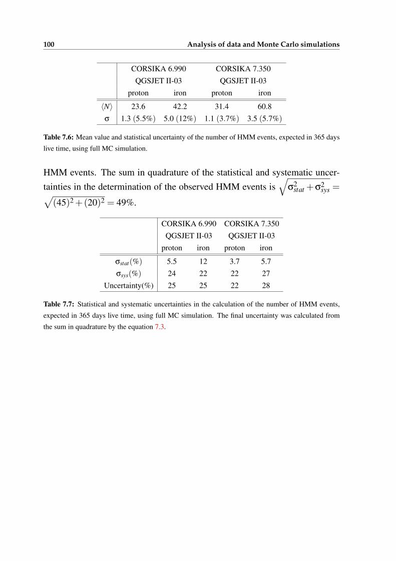
100 Analysis of data and Monte Carlo simulations

CORSIKA 6.990 CORSIKA 7.350

QGSJET II-03 QGSJET II-03

proton iron proton iron

〈N〉 23.6 42.2 31.4 60.8

σ 1.3 (5.5%) 5.0 (12%) 1.1 (3.7%) 3.5 (5.7%)

Table 7.6: Mean value and statistical uncertainty of the number of HMM events, expected in 365 days

live time, using full MC simulation.

HMM events. The sum in quadrature of the statistical and systematic uncer-tainties in the determination of the observed HMM events is

√σ2

stat +σ2sys =√

(45)2 +(20)2 = 49%.

CORSIKA 6.990 CORSIKA 7.350

QGSJET II-03 QGSJET II-03

proton iron proton iron

σstat(%) 5.5 12 3.7 5.7

σsys(%) 24 22 22 27

Uncertainty(%) 25 25 22 28

Table 7.7: Statistical and systematic uncertainties in the calculation of the number of HMM events,

expected in 365 days live time, using full MC simulation. The final uncertainty was calculated from

the sum in quadrature by the equation 7.3.

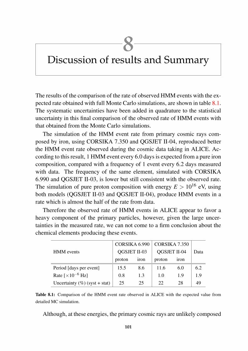
8Discussion of results and Summary

The results of the comparison of the rate of observed HMM events with the ex-pected rate obtained with full Monte Carlo simulations, are shown in table 8.1.The systematic uncertainties have been added in quadrature to the statisticaluncertainty in this final comparison of the observed rate of HMM events withthat obtained from the Monte Carlo simulations.

The simulation of the HMM event rate from primary cosmic rays com-posed by iron, using CORSIKA 7.350 and QGSJET II-04, reproduced betterthe HMM event rate observed during the cosmic data taking in ALICE. Ac-cording to this result, 1 HMM event every 6.0 days is expected from a pure ironcomposition, compared with a frequency of 1 event every 6.2 days measuredwith data. The frequency of the same element, simulated with CORSIKA6.990 and QGSJET II-03, is lower but still consistent with the observed rate.The simulation of pure proton composition with energy E > 1016 eV, usingboth models (QGSJET II-03 and QGSJET II-04), produce HMM events in arate which is almost the half of the rate from data.

Therefore the observed rate of HMM events in ALICE appear to favor aheavy component of the primary particles, however, given the large uncer-tainties in the measured rate, we can not come to a firm conclusion about thechemical elements producing these events.

CORSIKA 6.990 CORSIKA 7.350

HMM events QGSJET II-03 QGSJET II-04 Data

proton iron proton iron

Period [days per event] 15.5 8.6 11.6 6.0 6.2

Rate [×10−6 Hz] 0.8 1.3 1.0 1.9 1.9

Uncertainty (%) (syst + stat) 25 25 22 28 49

Table 8.1: Comparison of the HMM event rate observed in ALICE with the expected value from

detailed MC simulation.

Although, at these energies, the primary cosmic rays are unlikely composed

101

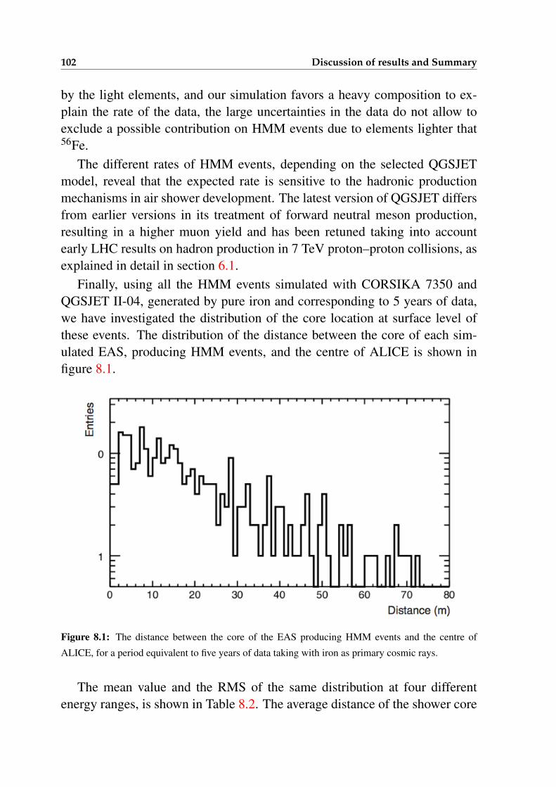
102 Discussion of results and Summary

by the light elements, and our simulation favors a heavy composition to ex-plain the rate of the data, the large uncertainties in the data do not allow toexclude a possible contribution on HMM events due to elements lighter that56Fe.

The different rates of HMM events, depending on the selected QGSJETmodel, reveal that the expected rate is sensitive to the hadronic productionmechanisms in air shower development. The latest version of QGSJET differsfrom earlier versions in its treatment of forward neutral meson production,resulting in a higher muon yield and has been retuned taking into accountearly LHC results on hadron production in 7 TeV proton–proton collisions, asexplained in detail in section 6.1.

Finally, using all the HMM events simulated with CORSIKA 7350 andQGSJET II-04, generated by pure iron and corresponding to 5 years of data,we have investigated the distribution of the core location at surface level ofthese events. The distribution of the distance between the core of each sim-ulated EAS, producing HMM events, and the centre of ALICE is shown infigure 8.1.

Figure 8.1: The distance between the core of the EAS producing HMM events and the centre of

ALICE, for a period equivalent to five years of data taking with iron as primary cosmic rays.

The mean value and the RMS of the same distribution at four differentenergy ranges, is shown in Table 8.2. The average distance of the shower core

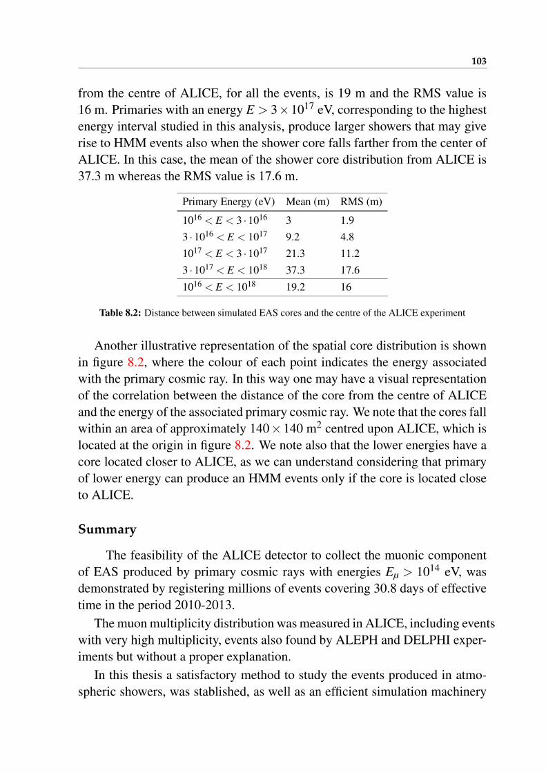
103

from the centre of ALICE, for all the events, is 19 m and the RMS value is16 m. Primaries with an energy E > 3×1017 eV, corresponding to the highestenergy interval studied in this analysis, produce larger showers that may giverise to HMM events also when the shower core falls farther from the center ofALICE. In this case, the mean of the shower core distribution from ALICE is37.3 m whereas the RMS value is 17.6 m.

Primary Energy (eV) Mean (m) RMS (m)

1016 < E < 3 ·1016 3 1.9

3 ·1016 < E < 1017 9.2 4.8

1017 < E < 3 ·1017 21.3 11.2

3 ·1017 < E < 1018 37.3 17.6

1016 < E < 1018 19.2 16

Table 8.2: Distance between simulated EAS cores and the centre of the ALICE experiment

Another illustrative representation of the spatial core distribution is shownin figure 8.2, where the colour of each point indicates the energy associatedwith the primary cosmic ray. In this way one may have a visual representationof the correlation between the distance of the core from the centre of ALICEand the energy of the associated primary cosmic ray. We note that the cores fallwithin an area of approximately 140×140 m2 centred upon ALICE, which islocated at the origin in figure 8.2. We note also that the lower energies have acore located closer to ALICE, as we can understand considering that primaryof lower energy can produce an HMM events only if the core is located closeto ALICE.

Summary

The feasibility of the ALICE detector to collect the muonic componentof EAS produced by primary cosmic rays with energies Eµ > 1014 eV, wasdemonstrated by registering millions of events covering 30.8 days of effectivetime in the period 2010-2013.

The muon multiplicity distribution was measured in ALICE, including eventswith very high multiplicity, events also found by ALEPH and DELPHI exper-iments but without a proper explanation.

In this thesis a satisfactory method to study the events produced in atmo-spheric showers, was stablished, as well as an efficient simulation machinery

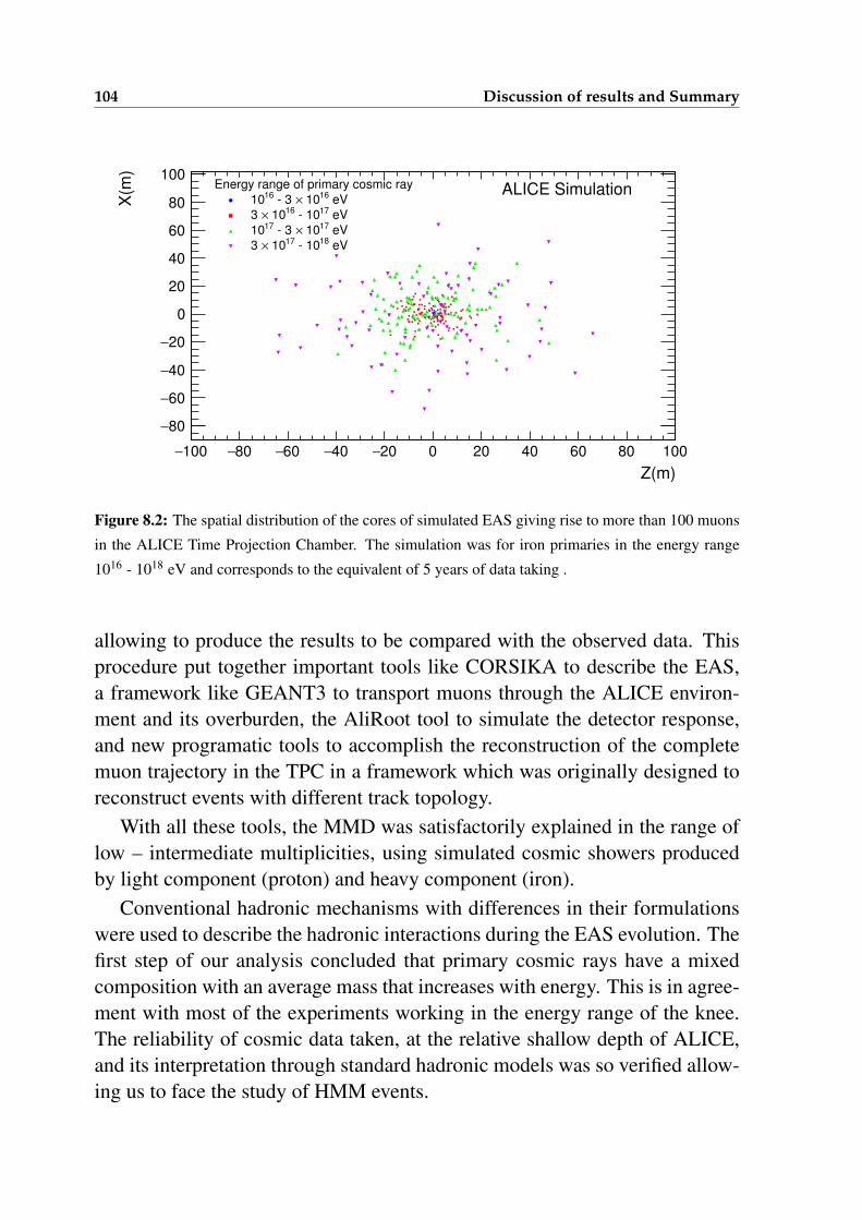
104 Discussion of results and Summary

Z(m)

100− 80− 60− 40− 20− 0 20 40 60 80 100

X(m

)

80−

60−

40−

20−

0

20

40

60

80

100Energy range of primary cosmic ray

eV16 10× ­ 3 1610

eV17 ­ 1016 10×3

eV17 10× ­ 3 1710

eV18 ­ 1017 10×3

ALICE Simulation

Figure 8.2: The spatial distribution of the cores of simulated EAS giving rise to more than 100 muons

in the ALICE Time Projection Chamber. The simulation was for iron primaries in the energy range

1016 - 1018 eV and corresponds to the equivalent of 5 years of data taking .

allowing to produce the results to be compared with the observed data. Thisprocedure put together important tools like CORSIKA to describe the EAS,a framework like GEANT3 to transport muons through the ALICE environ-ment and its overburden, the AliRoot tool to simulate the detector response,and new programatic tools to accomplish the reconstruction of the completemuon trajectory in the TPC in a framework which was originally designed toreconstruct events with different track topology.

With all these tools, the MMD was satisfactorily explained in the range oflow – intermediate multiplicities, using simulated cosmic showers producedby light component (proton) and heavy component (iron).

Conventional hadronic mechanisms with differences in their formulationswere used to describe the hadronic interactions during the EAS evolution. Thefirst step of our analysis concluded that primary cosmic rays have a mixedcomposition with an average mass that increases with energy. This is in agree-ment with most of the experiments working in the energy range of the knee.The reliability of cosmic data taken, at the relative shallow depth of ALICE,and its interpretation through standard hadronic models was so verified allow-ing us to face the study of HMM events.

105

As a second step, our analysis stated that only events produced by primaryelements with energies above 1016 eV give rise to HMM events (Nµ > 100).Then, a large amount of simulated data, corresponding to one year of live timewere generated both with proton and iron primaries, to reduce the fluctuationsin the rate of HMM events, in the energy range 1016 < E < 1018 eV.

The last step was the study of the observed rate of the HMM events. Weconcluded that this rate (5 events in 30.8 days) is well described by the pre-dicted rate from Monte Carlo simulations using CORSIKA 7.350 and QGSJETII-04, by assuming a heavy composition at energies E > 1016 eV.

The limited period of data taking (30.8 days) and the very low rate of HMMevents, give rise to a large uncertainty in the measured rate of these events (al-most 50%), preventing us from strong conclusions about the elements produc-ing these events, although heavy nuclei are the most probable. Therefore, anexplanation of the rate of HMM events, using a reasonable heavy compositionand a description of the EAS given by conventional hadronic mechanisms, isfor the first time compatible with the observed data.

Our results seem to be compatible with a knee of the energy spectrum dueto the light composition followed by a spectral steepening of the other ele-ments depending on their atomic number Z.

Bibliography

[1] ALICE Collaboration, K. Aamodt et al., “The ALICE experiment atthe CERN LHC,” JINST 3 no. 8, (2008) S08002.

[2] Y. Akiba et al., “The Hot QCD White Paper: Exploring the Phases ofQCD at RHIC and the LHC,” (2015) , arXiv:1502.02730[nucl-ex].

[3] J. Alme et al., “The ALICE TPC, a large 3-dimensional trackingdevice with fast readout for ultra-high multiplicity events,” Nucl.Instrum. Meth. A 622 (2010) 316–367, arXiv:1001.1950[physics.ins-det].

[4] M. Aglietta et al., “The EAS size spectrum and the cosmic ray energyspectrum in the region 1015-1016 eV,” Astropart. Phys. 10 no. 1,(1999) 1–9.

[5] M. A. K. Glasmacher et al., “The cosmic ray composition between1014 and 1016 eV,” Astropart. Phys. 12 no. 1, (1999) 1–17.

[6] T. Antoni et al., “Electron, muon, and hadron lateral distributionsmeasured in air showers by the KASCADE experiment,” Astropart.Phys. 14 no. 4, (2001) 245–260.

[7] G. Battistoni et al., “Cosmic-muon results from the NUSEXexperiment,” Il Nuovo Cimento C 9 no. 2, (1986) 196–209, 0390-5551.

[8] M. Ambrosio et al., “Vertical muon intensity measured with MACROat the Gran Sasso laboratory,” Phys. Rev. D 52 no. 7, (1995)3793–3802.http://link.aps.org/doi/10.1103/PhysRevD.52.3793.

[9] P. Kuusiniemi et al., “Underground cosmic-ray experiment EMMA,” J.Phys.: Conf. Ser. 409 no. 1, (2013) 012067.http://stacks.iop.org/1742-6596/409/i=1/a=012067.

107

108 Bibliography

[10] HiRes Collaboration, D. J. Bird et al., “The Cosmic Ray spectrumobserved by Fly’s Eye,” Astrophys. J. 424 (1994) 491–502.

[11] Pierre Auger Collaboration, R. W. Cronin, “The Pierre AugerObservatory Design Report (2nd edition),” Nucl. Phys. B, Proc. Suppl.28B (1998) 213. http://www.auger.org.

[12] KASCADE-Grande Collaboration, W. D. Apel et al., “The spectrumof high-energy cosmic rays measured with KASCADE-Grande,”Astrop. Phys. 36 (2012) 183–194, arXiv:1206.3834[astro-ph.HE].

[13] Telescope Array Collaboration, P. Tinyakov, “Latest results from theTelescope Array,” Nucl. Instrum. Meth. A 742 no. 067, (2014) 29–34.

[14] C. Grupen et al., “Measurements of the muon component of extensiveair showers at 320 m.w.e. underground,” Nucl. Instrum. Meth. 510no. 1-2, (2003) 190–193.

[15] DELPHI Collaboration, J. Ridky and P. Travnicek, “Detection ofmuon bundles from cosmic ray showers by the DELPHI experiment,”Nucl. Phys. B, Proc. Suppl. 138 (2005) 295–298.

[16] L3 Collaboration, P. Achard et al., “Measurement of the atmosphericmuon spectrum from 20-GeV to 3000-GeV,” Phys. Lett. B598 (2004)15–32, hep-ex/0408114 [nucl-ex].

[17] “LEP Design Report: Vol. 2. The LEP Main Ring,” (1984) .

[18] S. Ostapchenko, “QGSJET-II: Towards reliable description of veryhigh energy hadronic interactions,” Nucl. Phys. B, Proc. Suppl. 151(2006) 143–146, arXiv:hep-ph/0412332 [hep-ph].

[19] S. Ostapchenko, “Monte Carlo treatment of hadronic interactions inenhanced Pomeron scheme: I. QGSJET-II model,” Phys. Rev. D 83no. 1, (2011) 014018, arXiv:1010.1869 [hep-ph].

[20] D. Pacini, “La radiazione penetrante alla superficie ed in seno alleacque,” Nuovo Cim. Serie VI, Tomo 3 (1912) 93–100.

[21] V. F. Hess, “Uber Beobachtungen der durchdringenden Strahlung beisieben Freiballonfahrten,” Phys. Zeitschr. 13 (1912) 1084–1091.

Bibliography 109

[22] R. A. Millikan and G. H. Cameron, “High frequency rays of cosmicorigin,” Phys. Rev. 28 no. 68, (1926) 851.

[23] W. Bothe and W. Kolhorster, “Das Wesen der Hohenstrahlung,” Phys.Zeitschr. 56 (1929) 751–777.

[24] D. V. Skobelzyn, “Uber eine Neue Art sehr schneller Beta-Strahlen,” Z.Phys. 54 (1929) 686–703.

[25] P. Auger et al., “Extensive Cosmic-Ray Showers,” Rev. Mod. Phys. 11(1939) 288.

[26] Particle Data Group Collaboration, S. Eidelman et al., “Review ofparticle physics. Particle Data Group,” Phys. Lett. B 592 (2004)1–1109.

[27] S. P. Swordy, “The energy spectra and anisotropies of cosmic rays,”Space. Sci. Rev. 99 (2001) 85–94.

[28] R. W. Clay, Z. Kurban, and N. R. Wild, “Cosmic Ray RelatedUndergraduate Experiments,” GAP Note 1998-061 (Technical andScientific Notes about the Pierre Auger Project) (1998) .

[29] J. W. Cronin, T. K. Gaisser, and S. P. Swordy, “Cosmic rays at theenergy frontier,” Sci. Am. 276 (1997) 32–37.

[30] J. Horandel, “Models of the knee in the Energy Spectrum of CosmicRays,” Astropart. Phys. 21 no. 3, (2004) 241–265,arXiv:astro-ph/0402356v2 [astro-ph].

[31] Particle Data Group Collaboration, J. Beringer et al., “Review ofParticle Physics (RPP),” Phys. Rev. D. 86 (2012) 010001.

[32] J. Simpson, “Elemental and isotopic composition of Galactic cosmicrays,” Annu. Rev. Nucl. Part. S. 33 (1983) 323–381.

[33] A. A. Watson, “EARLY UNIVERSE: Cosmologists Celebrate theDeath of Defects,” Science 278 (1997) 574.

[34] HiRes Collaboration, D. J. Bird et al., “Evidence for correlatedchanges in the spectrum and composition of cosmic rays at extremelyhigh-energies,” Phys. Rev. Lett. 71 (1993) 3401–3404.

110 Bibliography

[35] HiRes Collaboration, D. J. Bird et al., “Detection of a cosmic ray withmeasured energy well beyond the expected spectral cutoff due tocosmic microwave radiation,” Astrophys. J. 441 (1995) 144–150.

[36] D. Bindig, C. Bleve, and K.-H. Kampert, “Air shower development:impact of the LHC data,” Proceedings, 32nd International Cosmic RayConference (ICRC 2011) 1 (2011) 161–164.http://inspirehep.net/record/1346047/files/v1_1284.pdf.

[37] EAS-TOP Collaboration, B. Alessandro, “Study of the compositionaround the knee through the electromagnetic and muon detectors dataat EAS-TOP,” Proceedings of the 27th International Cosmic RayConference, Hamburg 1 (2001) 124.http://galprop.stanford.edu/elibrary/icrc/2001/proceedings/ICRC2001/he_index.html.

[38] EAS-TOP Collaboration, M. Aglietta et al., “The cosmic ray primarycomposition in the knee region through the EAS electromagnetic andmuon measurements at EAS-TOP,” Astropart. Phys. 21 (2004)583–596.

[39] EAS-TOP, MACRO Collaboration, M. Bertaina, “The Proton, Heliumand CNO Fluxes at E0 ∼= 100 TeV from the EAS-TOP (Cherenkov)and MACRO (TeV Muon) Data at the Gran Sasso Laboratories,”Proceedings of the 28th International Cosmic Ray Conference,Tsukuba 1 (2003) 115–118. http://www-rccn.icrr.u-tokyo.ac.jp/icrc2003/PROCEEDINGS/PDF/29.pdf.

[40] KASCADE Collaboration, T. Antoni et al., “KASCADEmeasurements of energy spectra for elemental groups of cosmic rays:Results and open problems,” Astropart. Phys. 24 no. 1, (2005) 1–25,arXiv:astro-ph/0505413 [astro-ph].

[41] Y. A. Fomin et al., “Nuclear composition of primary cosmic rays in the’knee’ region according MSU EAS array data,” J. Phys. G 22 (1996)1839–1849.

[42] O. A. Gress et al., “The study of primary cosmic rays energy spectrumand mass composition in the energy range 0.5-50PeV with TUNKA

Bibliography 111

EAS Cherenkov array,” Nucl. Phys. B, Proc. Suppl. 75 (1999)299–301.

[43] L. Sveshnikova et al., “Cosmic ray spectrum above the knee measuredby the Tunka-133 experiment: special features and possibleinterpretations,” Proceedings of the 33th International Cosmic RayConference, Rio de Janeiro (2014) 0304.http://www.cbpf.br/%7Eicrc2013/papers/icrc2013-0304.pdf.

[44] AMANDA, SPASE Collaboration, K. Rawlins, “Measurement of thecosmic ray composition at the knee with the SPASE-2/AMANDA-B10detectors,” Proceedings of the 28th International Cosmic RayConference, Tsukuba 1 (2003) 173–176. http://www-rccn.icrr.u-tokyo.ac.jp/icrc2003/PROCEEDINGS/PDF/44.pdf.

[45] M. A. K. Glasmacher et al., “Energy spectra and composition near theknee,” Nucl. Phys. Proc. Suppl. 75A (1999) 241–243.

[46] IceCube Collaboration, T. K. Gaisser, “Primary spectrum andcomposition with IceCube/IceTop,” Cosmic Ray InternationalSeminar: The status and the future of the UHE Cosmic Ray Physics inthe post LHC era (CRIS 2015) Gallipoli, Italy, September 14-16, 2015(2016) , arXiv:1601.06670 [astro-ph.HE]. http://www-rccn.icrr.u-tokyo.ac.jp/icrc2003/PROCEEDINGS/PDF/44.pdf.

[47] J. Horandel, “On the knee in the energy spectrum of cosmic rays,”Astropart. Phys. 19 no. 2, (2003) 193–220,arXiv:astro-ph/0210453 [astro-ph].

[48] E. G. Berezhko et al., “Composition of cosmic rays accelerated insupernova remnants,” J. Exp. Theor. Phys. 89 no. 3, (1999) 391–403.[Zh. Eksp. Teor. Fiz. 116, 737 (1999)].

[49] T. Stanev et al., “Cosmic rays. IV. The spectrum and chemicalcomposition above 10 GeV,” Astron. Astrophys. 274 (1993) 902,astro-ph/9303006.

[50] K. Kobayakawa et al., “Acceleration by oblique shocks at supernovaremnants and cosmic ray spectra around the knee region,” Phys. Rev. D66 no. 8, (2002) 083004, astro-ph/0008209.

112 Bibliography

[51] L. G. Sveshnikova, “The knee in the Galactic cosmic ray spectrum andvariety in Supernovae,” Astron. Astrophys. 409 (2003) 799–807,astro-ph/0303159.

[52] S. P. Swordy, “Expectations for Cosmic Ray Composition Changes inthe Region 10**14 to 10**16 eV,” Proceedings of the 24thInternational Cosmic Ray Conference, Rome 2 (1995) 697.

[53] A. A. Lagutin et al., “The “knee” in the primary cosmic ray spectrumas consequence of the anomalous diffusion of the particles in the fractalinterstellar medium,” Nucl. Phys. B, Proc. Suppl. 97 (2001) 267–270.

[54] V. S. Ptuskin et al., “Diffusion and drift of very high energy cosmicrays in galactic magnetic fields,” Astron. Astrophys. 268 no. 2, (1993)726–735.

[55] S. Ogio and F. Kakimoto, “Advective Diffusion Propagation Model forGalactic Cosmic Rays above 1012 eV,” Proceedings of the 28thInternational Cosmic Ray Conference, Tsukuba 1 (2003) 315–318.http://www-rccn.icrr.u-tokyo.ac.jp/icrc2003/PROCEEDINGS/PDF/80.pdf.

[56] J. Candia, S. Mollerach, and E. Roulet, “Cosmic ray spectrum andanisotropies from the knee to the second knee,” J. Cosmol. Astropart.Phys. 5 (2003) 003, astro-ph/0302082.

[57] D. Kazanas and A. Nicolaidis, “Cosmic Ray “Knee”: A Herald of NewPhysics?,” Proceedings of the 27th International Cosmic RayConference, Hamburg 5 (2001) 1760–1763,arXiv:astro-ph/0103147 [astro-ph].

[58] D. Kazanas and A. Nicolaidis, “Letter: Cosmic Rays and Large ExtraDimensions,” Gen. Relat. Gravit. 35 (2003) 1117–1123,hep-ph/0109247.

[59] M. Nagano and A. A. Watson, “Observations and implications of theultrahigh-energy cosmic rays,” Rev. Mod. Phys. 72 (2000) 689–732.

[60] K. Greisen, “End to the Cosmic-Ray Spectrum?,” Phys. Rev. Lett. 16(1966) 748–750.

Bibliography 113

[61] V. A. Kuzmin and G. T. Zatsepin, “On cosmic-ray interactions withprotons,” Can. J. Phys. 46 (1968) S617.

[62] R. A. Alpher, H. A. Bethe, and G. Gamow, “The Origin of ChemicalElements,” Phys. Rev. 73 (1948) 803–804.

[63] A. A. Penzias and R. W. Wilson, “A Measurement of Excess AntennaTemperature at 4080 Mc/s,” Astrophys. J. 142 (1965) 419–421.

[64] R. W. Clay, A. G. K. Smith, and J. L. Reid, “Cosmic ray induced noisein gravitational wave detectors,” Publ. Astron. Soc. Aust 14 (1997) 195.

[65] A. Haungs et al., “KCDC - The KASCADE Cosmic-ray Data Centre,”J. Phys. Conf. Ser. 632 no. 1, (2015) , arXiv:1504.06696[astro-ph.IM].

[66] MASS91 Collaboration, R. Bellotti, “Balloon measurements of cosmicray muon spectra in the atmosphere along with those of primaryprotons and helium nuclei over midlatitude,” Phys. Rev. D 60 (1999)052002, arXiv:hep-ex/9905012 [hep-ex].

[67] K. Greisen, “Cosmic Ray Showers,” Ann. Rev. Nucl. Sci. 10 (1960) 63.

[68] M. Nagano et al., “Energy spectrum of primary cosmic rays between1014.5 and 1018 eV,” J. Phys. G 10 (1984) 1295–1310.

[69] M. P. Pascale et al., “Absolute spectrum and charge ratio of cosmic raymuons in the energy region from 0.2 GeV to 100 GeV at 600 m abovesea level,” J. Geophys. Res-Space 98 (1993) 3501–3507.

[70] P. K. F. Grieder, “Cosmic Rays at the Earth,” Elsevier Science (2001) .

[71] S. Cecchini and M. Spurio, “Atmospheric muons: experimentalaspects,” Geosci. Instrum. Method. Data Syst. 1 (2012) 185–196,arXiv:1208.1171.

[72] B. C. Rastin, “An accurate measurement of the sea-level muonspectrum within the range 4 to 3000 GeV/c,” J. Phys. G Nucl. Part. 10(1984) 1609–1628.

[73] C. A. Ayre et al., “Precise measurement of the vertical muon spectrumin the range 20-500 GeV/c,” J. Phys. G Nucl. Part. 1 (1975) 584–600.

114 Bibliography

[74] H. Jokisch et al., “Cosmic-ray muon spectrum up to 1 TeV at 75degzenith angle,” Phys. Rev. D. 19 (1979) 1368–1372.

[75] K. P. Beuermann and G. Wibberenz, “Secondary spectra of electronsand photons in the atmosphere,” Can. J. Phys. 46 (1968) S1034.

[76] D. E. Groom et al., “Muon stopping-power and range tables 10-MeVto 100-TeV,” Atom. Data Nucl. Data Tabl. 78 (2001) 183–356.

[77] Y. Takahashi, “Elemental Abundance of High Energy Cosmic Rays,”Nucl. Phys. B, Proc. Suppl. 60 (1998) 83–92.

[78] RUNJOB Collaboration, M. Hareyama et al., “High Energy GalacticCosmic Rays Observed by RUNJOB Experiment,” J. Phys. Conf. Ser.31 (2006) 159–160.

[79] BESS Collaboration, T. Sanuki, “Cosmic ray data and theirinterpretation: About BESS experiment,” Nucl. Phys. Proc. Suppl.175-176 (2008) 149–154.

[80] CAPRICE Collaboration, T. Mocchiutti, “Composition of cosmic rayparticles in the atmosphere as measured by the CAPRICE98 balloonborne apparatus,” Proceedings of the 28th International Cosmic RayConference, Tsukuba 1 (2003) 1627–1630.

[81] S. Coutu et al., “Cosmic ray positrons: Are there primary sources?,”Astropart. Phys. 11 (1999) 429–435, arXiv:astro-ph/9902162[astro-ph].

[82] A. D. Panov, V. I. Zatsepin, and N. V. Sokolskaya, “Spectra ofabundant nuclei in sources, according to the ATIC experiment,” Bull.Russ. Acad. Sci. Phys. 79 no. 3, (2015) 285–288. [Izv. Ross. Akad.Nauk Ser. Fiz.79,no.3,318–321(2015)].

[83] CREAM Collaboration, H. S. Ahn et al., “Measurements of therelative abundances of high-energy cosmic-ray nuclei in theTeV/nucleon region,” Astrophys. J 715 (2010) 1400–1407.

[84] PAMELA Collaboration, W. Menn et al., “PH, He, Li and Be Isotopesin the PAMELA-Experiment,” J. Phys. Conf. Ser. 675 (2016) 032001.

Bibliography 115

[85] A. Chiavassa et al., “KASCADE-Grande: The Grande array,”Proceedings of the 28th International Cosmic Ray Conference,Tsukuba (2003) 989–992. http://www-rccn.icrr.u-tokyo.ac.jp/icrc2003/PROCEEDINGS/PDF/248.pdf.

[86] Tibet ASgamma Collaboration, M. Amenomori et al., “Cosmic-rayenergy spectrum around the knee observed with the Tibet air-showerexperiment,” Astrophys. Space Sci. Trans. 7 (2011) 15–20.

[87] HiRes-MIA Collaboration, T. Abu-Zayyad et al., “Measurement of thecosmic ray energy spectrum and composition from 10**17-eV to10**18.3-eV using a hybrid fluorescence technique,” Astrophys. J. 557(2001) 686, arXiv:astro-ph/0010652 [astro-ph].

[88] AGASA Collaboration, M. Takeda et al., “Extension of the cosmic-rayenergy spectrum beyond the predicted Greisen-Zatsepin-Kuzmincutoff,” Phys. Rev. Lett. 81 (1998) 1163, arXiv:astro-ph/9807193[astro-ph].

[89] HiRes Collaboration, D. R. Bergman, “Observation of the GZK Cutoffby the HiRes Experiment,” Proceedings of the 30th InternationalCosmic Ray Conference 4 (2007) 451–454.http://indico.nucleares.unam.mx/contributionDisplay.py?contribId=1128&confId=4.

[90] AGASA Collaboration, K. Shinozaki, “AGASA results,” Nucl. Phys.Proc. Suppl. 151 (2006) 3–10.

[91] Pierre Auger, Telescope Array Collaboration, R. W. Cronin, “PierreAuger Observatory and Telescope Array: Joint Contributions to the34th International Cosmic Ray Conference (ICRC 2015),”FERMILAB-CONF-15-495-AD-AE-CD-TD (2015) ,arXiv:1511.02103 [astro-ph.HE].

[92] EAS-TOP, LVD Collaboration, M. Aglietta et al., “The high muonspectrum in Extensive Air Showers: first data from LVD andEAS-TOP at Gran Sasso,” Astrop. Phys. 9 (1998) 185–192.

[93] MACRO, EAS-TOP Collaboration, M. Aglietta, M. Ambrosio, et al.,“The Primary cosmic ray composition between 10**15 and 10**16 eV

116 Bibliography

from extensive air showers electromagnetic and TeV muon data,”Astropart. Phys. 20 (2004) 641–652, arXiv:astro-ph/0305325[astro-ph].

[94] S. M. Kasahara et al., “Study of cosmic ray composition in the kneeregion using multiple muon events in the Sudan 2 detector,” Phys. Rev.D 55 (1997) 5282.

[95] V. N. Batakanov, R. V. Novoseltsev, and R. V. Novoseltseva,“Detection of muon groups with multiplicity nµ > 1500 at the Baksanunderground scintillation telescope,” Astropart. Phys. 8 (1997) 59–66.

[96] A. G. Bogdanov and other, “Energy spectrum of cosmic ray muons in100 TeV energy region reconstructed from the BUST data,” Astropart.Phys. 36 (2012) 224–236, arXiv:0911.1692 [astro-ph.HE].

[97] T. Enqvist et al., “EMMA: A new underground cosmic-rayexperiment,” Nucl. Phys. Proc. Suppl. 175-176 (2008) 307–310.

[98] A. Ball et al., “Search for cosmic ray coincidences with detectors inthe LEP tunnel,” Astropart. Phys. (1994) 513–523.

[99] CMS Collaboration, V. Khachatryan et al., “Measurement of thecharge ratio of atmospheric muons with the CMS detector,” Phys. Lett.B692 no. 2, (2010) 83–54.

[100] CosmoALEPH Collaboration, A. S. Muller, “Status of theCOSMOLEP project,” Nucl. Phys. B, Proc. Suppl. 52B (1997)261–263.

[101] V. Avati et al., “Cosmic multi-muon events observed in theunderground CERN-LEP tunnel with the ALEPH experiment,”Astropart. Phys. 19 (2003) 513–523.

[102] N. N. Kalmykov and S. S. Ostapchenko, “The nucleus-nucleusinteraction, nuclear fragmentation, and fluctuations of extensive airshowers,” Phys. Atom. Nucl. 56 no. 3, (1993) 346–353. Yad. Fiz. 56(1993) 105-119.

[103] DELPHI Collaboration, J. Abdallah et al., “Study of multi-muonbundles in cosmic ray showers detected with the DELPHI detector at

Bibliography 117

LEP,” Astropart. Phys. 28 (2007) 273–286, arXiv:0706.2561[astro-ph].

[104] O. C. Allkofer, W. D. Carstensen, and W. D. Day, “The absolutecosmic ray muon spectrum at sea level,” Phys. Lett. B. 36 (1971)425–427.

[105] CMS Collaboration, S. Chatrchyan et al., “The CMS experiment at theCERN LHC,” JINST 3 no. 8, (2008) S08001.

[106] P. A. Schreiner, J. Reichenbacher, and M. C. Goodman, “Interpretationof the underground muon charge ratio,” Astrop. Phys. 32 no. 1, (2009)61–71. http://www.sciencedirect.com/science/article/pii/S0927650509000875.

[107] L3 Collaboration, B. Adeva et al., “The construction of the L3experiment,” Nucl. Instrum. Meth. A 289 (1990) 35–102.

[108] A. Akindinov et al., “Performance of the ALICE Time-Of-Flightdetector at the LHC,” Eur. Phys. J. Plus 128 no. 4, (2013) 44.

[109] E. Cuautle et al., “ACORDE, The ALICE cosmic ray detector,”Proceedings of the 30th International Cosmic Ray Conference 5(2008) 1201–1204.

[110] R. Santoro et al., “The ALICE Silicon Pixel Detector: readiness for thefirst proton beam,” J. Instrum. 4 no. 03, (2009) P03023.

[111] ALICE Collaboration, “ALICE Technical Design Report of theTrigger, Data Acquisition, High-Level Trigger, Control System,”.http://edms.cern.ch/document/456354/2.

[112] C. Richards-Serre, “Evaluation de la perte d’energie unitaire et duparcours pour des muons de 2 a 600-GeV dans un absorbantquelconque,” Technical Report CERN-71-18 (1971) .

[113] ALICE Collaboration, B. Abelev et al., “Performance of the ALICEexperiment at the CERN LHC,” Int. J. Mod. Phys. A 29 no. 24, (2014)1430044, arXiv:1402.4476 [nucl-ex].

[114] P. Billoir, “Progressive track recognition with a Kalman like fittingprocedure,” Comput. Phys. Commun. 57 (1989) 390–394.

118 Bibliography

[115] D. Heck et al., “CORSIKA: A Monte Carlo code to simulate extensiveair showers,” FZKA-6019 (1998) .http://bibliothek.fzk.de/zb/berichte/FZKA6019.pdf.

[116] KASCADE Collaboration, T. Antoni et al., “The cosmic rayexperiment KASCADE,” Nucl. Instr. Meth. A 513 (2003) 490–510.

[117] D. Heck and T. Pierog, “Extensive air shower simulation withCORSIKA: A User’s Guide (Version 6.99x from August 8, 2011),”.http://www-ik.fzk.de/˜corsika.

[118] D. Heck and T. Pierog, “Extensive air shower simulation withCORSIKA: A User’s Guide (Version 7.350 from December, 2012),”.http://www-ik.fzk.de/˜corsika.

[119] J. Ranft, “DPMJET version II.5: Sampling of hadron hadron,hadron-nucleus and nucleus-nucleus interactions at accelerator andcosmic ray energies according to the two component dual partonmodel: Code manual,” SI-99-6 (1999) , arXiv:hep-ph/9911232[hep-ph].

[120] K. Werner et al., “Parton ladder splitting and the rapidity dependenceof transverse momentum spectra in deuteron-gold collisions at RHIC,”Phys. Rev. C 74 (2006) 044902, arXiv:hep-ph/0506232 [hep-ph].

[121] H. J. Drescher et al., “Parton-Based Gribov-Regge Theory,” Phys.Rept. 350 (2001) 93–289, arXiv:hep-ph/0007198 [hep-ph].

[122] R. S. Fletcher et al., “SYBILL: An event generator for simulation ofhigh-energy cosmic ray cascades,” Phys. Rev. D 50 (1994) 5710–5731.

[123] K. Werner et al., “Strings, pomerons, and the VENUS model ofhadronic interactions at ultra relativistic energies,” Phys. Rept. 232(1993) 87–299.

[124] A. B. Kaidalov and K. A. Ter-Martirosyan, “Multiple production ofhadrons at high-energies in the model of Quark-Gluon String,” Sov. J.Nucl. Phys. 39 (1984) 979–1028. Yad. Fiz. 39 (1984) 1545-1558.

[125] S. Ostapchenko, “Air shower development: impact of the LHC data,”Proceedings, 32nd International Cosmic Ray Conference (ICRC 2011)

Bibliography 119

2 (2011) 71.http://inspirehep.net/record/1352304/files/v2_0681.pdf.

[126] R. Brun et al., “GEANT Detector Description and Simulation Tool,”CERN Programming Library Long Writeup W5013 (1994) .