Embed Size (px)
Citation preview
Study of polymer film formation
and their characterization using
NMR, XRD and DSC
Dissertation
zur Erlangung des akademischen Grades
doctor rerum naturalium (Dr. rer. nat.)
Vorgelegt dem Rat der
Fakultät für Mathematik und Naturwissenschaften
der Technischen Universität Ilmenau
von
M. Sc. Sushanta Ghoshal
geboren am 31.01.1980 in Dhaka, Bangladesch
Berichter: Universitätsprofessor Prof. Dr. rer. nat. habil. Siegfried Stapf
urn:nbn:de:gbv:ilm1-2012000151

Promotionskomission
Vorsitzender: Prof. Dr. Erich Runge
(Institut für Physik, TU Ilmenau)
Gutachter: Prof. Dr. rer. nat. habil. Siegfried Stapf (Institut für Physik, TU Ilmenau)
Prof. Dr. rer. nat. habil. Uwe Ritter (Institut für Chemie und Biotechnik, TU Ilmenau)
Prof. Dr. Ioan Ardelean (Technical University of Cluj-Napoca, Romania)
weitere Mitglieder: Prof. Dr. Jörg Kröger (Institut für Physik, TU Ilmenau)
PD Dr. rer. nat. habil. Paul Denner (Institut für Physik, TU Ilmenau)
Tag des Einreichung: 05. December 2011
Tag der wissenschaftlichen Aussprache: 07. March 2012
Study of polymer film formation and
their characterization using NMR,
XRD and DSC
Dissertation
In partial fulfillment of the
requirements for the degree of
doctor rerum naturalium (Dr. rer. nat.)
at the Faculty of Mathematics and Natural Science,
Ilmenau University of Technology
By
M. Sc. Sushanta Ghoshal
Born on 31.01.1980 in Dhaka, Bangladesh
Supervisor: Universitätsprofessor Prof. Dr. rer. nat. habil. Siegfried Stapf
Ilmenau, Germany
To my parents
I
Untersuchung und Charakterisierung der Bildung von
Polymerschichten mit Hilfe von NMR, XRD und DSC
Zusamenfassung
Die Bildung dünner Polymerschichten aus den umweltfreundlichen Polymeren Gelatine,
Stärke und Poly(vinylalkohol) (PVOH) wurde mit Hilfe von Kernspinresonanz (NMR),
Weitwinkel-Röntgendiffraktometrie (XRD) und Differential-Scanning-Kalorimetrie (DSC)
untersucht. Die Proben wurden durch Abguss wässriger Polymerlösungen hergestellt und
ihr Trocknungsprozess bei Raumtemperatur mit Hilfe eines unilateralen NMR-Scanners
bis zur vollständigen Erstarrung untersucht. Eindimensionale Tiefenprofile mit
mikroskopischer Auflösung wurden zu verschiedenen Stadien des Prozesses
aufgenommen. Jeder Profilpunkt wurde dabei aus der Summe mehrerer Spin-Echos
gebildet. Weiterhin wurden aus der Abnahme der Echointensitäten für jeden Punkt Spin-
Spin-Relaxationszeiten (2T ) bestimmt und in Bezug auf den Trocknungsprozess
interpretiert. Darüber hinaus wurden Spin-Gitter-Relaxationszeiten (1T ) gemessen.
Abhängig vom Typ und der ursprünglichen Konzentration des untersuchten Polymers
wurden während der Verdunstung des Lösungsmittels unterschiedliche
molekulardynamische Prozesse in verschiedenen Tiefen der Schicht beobachtet. Die
Ergebnisse zeigen eine räumliche Inhomogenität der molekulardynamischen Prozesse
während der Trocknung. Im fortgeschrittenen Stadium des Trocknungsprozesses
beeinflusst diese Inhomogenität die mikroskopische Anordnung der Polymerketten
während der Erstarrung und bestimmt somit die endgültige Struktur der Polymerschicht.
XRD-Messungen der vollständig erstarrten Schichten bestätigen die von den NMR-
Messungen aufgezeigte strukturelle Inhomogenität.

II
III
Study of polymer film formation and their characterization
using NMR, XRD and DSC
Abstract
Film formation and their characterization of three eco-friendly polymers, namely gelatin,
starch and poly(vinyl alcohol) (PVOH) were studied using nuclear magnetic resonance
(NMR), wide-angle X-ray diffractometry (XRD) and differential scanning calorimetry (DSC)
techniques. Polymer solutions were prepared using water as a solvent followed by
casting. The drying process of the cast sample was monitored at room temperature with a
single-sided NMR scanner until complete solidification occurred. Depth-dependent NMR
profiles with microscopic resolution were acquired at different stages of sample drying.
Each profile point was accumulated from the echo decay. Spin-spin relaxation times (2T )
were measured from the echo decays at different layers and were correlated with the
drying process during film formation. Additionally, spin-lattice relaxation times (1T ) were
determined. Depending on the polymer studied and the initial concentration of each
polymer, different types of molecular dynamics were observed at different heights during
evaporation of the solvent. The study indicates that each polymer shows a spatial
heterogeneity in the molecular dynamics during drying. In the advanced stage of drying
process, the microscopic arrangement of the polymer chains during their solidification is
influenced by this dynamic heterogeneity and determines the final structure of the film.
XRD of the film in its final state confirmed the structural heterogeneity identified by the
NMR.

IV
V
Contents
Zusamenfassung .................................................................................................................................. I
Abstract ............................................................................................................................................. III
Contents ............................................................................................................................................. V
1. Introduction ........................................................................................................................ 1
2. Methods and Theoretical Background .................................................................................. 5
2.1 Nuclear Magnetic Resonance (NMR) .................................................................................... 5
2.2 X-ray Diffractometry (XRD).................................................................................................. 14
2.3 Differential Scanning Calorimetry (DSC) ............................................................................. 15
3. Experimental .................................................................................................................... 17
3.1. Materials .............................................................................................................................. 17
3.1.1. Introduction of the polymers ..................................................................................... 17
3.1.2. Materials used in this study ....................................................................................... 21
3.2. Methods ............................................................................................................................... 23
3.2.1. Sample preparation ................................................................................................... 23
3.2.2. Casting ........................................................................................................................ 24
3.3. Instrumentation ................................................................................................................... 25
4. Study of gelatin film formation and its characterization ..................................................... 31
4.1. Introduction ......................................................................................................................... 31
4.2. Samples ................................................................................................................................ 32
4.3. Film formation study ............................................................................................................ 34
4.3.1. Real time film formation study using single-sided NMR scanner .............................. 34
4.3.2. Gelatin film formation study using high-field NMR and DSC ..................................... 45
4.3.3. Determination of evaporation tendency ................................................................... 50
4.4. Film characterization............................................................................................................ 51
Contents VI
4.4.1. Single-sided NMR study ............................................................................................. 51
4.4.2. XRD study ................................................................................................................... 52
4.4.3. DSC study ................................................................................................................... 54
4.5. Proposed Mechanism of gelatin film formation .................................................................. 55
4.6. Concentration and humidity effects on gelatin films .......................................................... 58
4.7. Conclusions .......................................................................................................................... 64
5. Starch film formation study ............................................................................................... 66
5.1. Introduction ......................................................................................................................... 66
5.2. Samples ................................................................................................................................ 67
5.3. Film formation study using micro camera ........................................................................... 68
5.4. Real time film formation study using single-sided NMR scanner ........................................ 70
5.5. Film characterization............................................................................................................ 80
5.5.1. Single-sided NMR study ............................................................................................. 80
5.5.2. XRD study ................................................................................................................... 81
5.6. Proposed mechanism of starch film formation ........................................................................ 82
5.7. Conclusions .......................................................................................................................... 84
6. Structural and dynamical heterogeneities of PVOH film during its formation ...................... 86
6.1. Introduction ......................................................................................................................... 86
6.2. Samples ................................................................................................................................ 87
6.3. Film formation study ............................................................................................................ 89
6.3.1. Real time film formation study using single-sided NMR scanner .............................. 89
6.3.2. NMR study at 40 MHz .............................................................................................. 102
6.3.3. NMR study using Field cycling relaxometer ............................................................. 104
6.4. Film characterization.......................................................................................................... 105
6.4.1. Single-sided NMR study ........................................................................................... 105
6.4.2. XRD study ................................................................................................................. 106
6.5. Proposed mechanism of PVOH film formation .................................................................. 109
6.6. Conclusions ........................................................................................................................ 110
7. Summary and outlook ..................................................................................................... 112
Publications by the Author as a part of this work .......................................................................... 115
Bibliography ................................................................................................................................... 116
Acknowledgements ........................................................................................................................ 128
Curriculum Vitae ……………………………………………………………………………………………………………………… 129

1
Chapter 1
Introduction
Who has begun has half done.
Have the courage to be wise. Begin!
Quintus Horatius Flaccus
In this modern era, polymers touch our lives from the daily household materials to
the sophisticated artificial heart. According to their origin, polymers can be grouped as
natural or synthetic. Synthetic polymers are established and abundantly used mainly due
to their low price, availability, physical and chemical properties. However, they are
responsible for producing enormous amount of waste in daily life, a problem of ever
growing importance to mankind. Furthermore, the future availability of fossil resources,
which is the nonrenewable source of synthetic polymer, is said to be restricted within a
practical time scale. In contrast, biopolymers originated from natural resources have
inherent properties, unique functionality and applicability. Consequently, it is worthwhile to
explore the new applications of biopolymers as an alternative of synthetic type petroleum
based polymers, which not only will protect the environment but also make use of our
most abundant renewable resources. There are two main classes of biopolymers, for
example, those which are obtained from the plant origin (cellulose, starch, alginate, etc.)
and those which are obtained from the animal sources (gelatin, shellac, chitosan, etc.) [1]-
[4].
In our daily life we are exposed to myriad applications of polymer films, for
instance, food wrapping, the packaging of various items, protective coating on the surface
of materials and so on. Over the past few decades impressive advances have been made
in the production and application of these films which are mainly synthetic in nature. In
Chapter 1: Introduction 2
recent years, biopolymer films are showing promising aspects in different applications as
mentioned above [3]-[5]. Moreover, films obtained from biopolymers and environmentally
friendly synthetic polymers find potential applications even in the biomedical and
biotechnological fields. These include biocompatible coatings, thin films for tissue
engineering and drug delivery [6]. However, biopolymer films have some inherent
properties like hydrophobicity, low mechanical properties and aging which are not suitable
for most of their applications [7]-[9]. Widespread works have been performed to diminish
these shortcomings by modification of the films for different applications. At the same
time, mechanical, thermal, electrical and structural properties of different biopolymer films
have been studied [3], [4], [10]. Despite these extensive studies on films, not much
attention has been given to studying the film formation process. The drying process during
the formation of the polymer film is important because the final structure and the
characteristic properties of the film depend on this process [11]. The conformation of the
polymer chains, as well as their dynamical properties, change during drying as the solvent
evaporates. Note that non-uniform drying takes place in many processes of film formation
as it can be seen in different colloidal systems like latex dispersions and paints [12]-[14].
In case of biopolymer, information which can be acquired from the film formation study
may have an enormous implication in the application and tailoring of the film.
The aim of this thesis is to study, for the first time to the best of our knowledge, the
drying process during the biopolymer film formation using NMR technique. To accomplish
this goal, two biopolymers are selected based on their sources. Due to difference in
chemical structure and the properties when mixed with water, unlike molecular dynamics
during the film formation of these biopolymers is presumed. Firstly, gelatin [15] is chosen
which is one of the abundant natural biopolymer from animal origin and has a complex
structure. Different amino acids are the repeating unit in this biopolymer. Gelatin forms gel
or solution in water when dissolved depending on the initial concentration. Starch [16] is
the second biopolymer which is used to study the film formation in this thesis. It is the
second most abundant natural biopolymer after cellulose from plant origin having glucose
unit as the monomer. On the contrary to gelatin, starch forms suspension when mixed
with water.
To study the film formation of a polymer having relatively simple structure
compared to the complex structure of the biopolymer, poly(vinyl alcohol) (PVOH) [17], a
synthetic but environmentally friendly polymer is chosen. Since the proper modification of
the biopolymers is yet to achieve a certain level to compete with the synthetic polymers,
increasing interest on the use of eco-friendly synthetic polymers as like as PVOH are
developing. PVOH forms viscous solution when it is dissolved in water. In contrast with
Chapter 1: Introduction 3
gelatin and starch samples, the film formation of PVOH has been studied previously using
different approaches [11], [18]-[22].
In this study, low-field nuclear magnetic resonance (NMR) technique is used to
follow the drying process in terms of relaxation behavior of the sample. In recent years,
low field [23] as well as high field [24]-[26] NMR techniques have been employed to
characterize biopolymer gels and films. On the other hand, there are few experimental
techniques, for instance, atomic force microscopy (AFM), spectroscopic ellipsometry, X-
ray photoelectron spectroscopy (XPS), X-ray diffractometry (XRD) or ultrasound reflection
that have been employed in order to follow the film formation of different polymer or
inorganic materials [27]-[30], but none of them offers a spatially resolved dynamical
information as well as density profiling at the same time which are employed in this study
using low-field single-sided NMR scanner. A single-sided NMR scanner combines the
open magnets and surface radio frequency (RF) coils to generate a magnetic field to
measure an object external to the scanner and inside the object under investigation [31].
In this study, the main advantage of using low-field NMR scanner over the conventional
high-field NMR spectrometer is its capability to extract a manifold of information during
depth dependent in situ film formation study without interrupting the drying process. X-Ray
diffractometry (XRD), which is capable of providing information on the structure of the final
state of a film at a molecular level, is used to characterize the dried polymer films. The
thermal properties of the films are investigated using differential scanning calorimetry
(DSC). XRD and DSC studies of the film in its final state strengthen our results as
observed during the film formation study using NMR technique.
The structure of this dissertation is as follows.
In chapter 2 the theoretical backgrounds of the methods used in this study are
introduced. In this context, firstly, the basic of NMR from the semi-classical point of view is
described along with the relaxation mechanism of the nuclear spin system. The particular
pulse sequences used in this study are presented. Later on, without going in great detail,
the basics of XRD and operational technique of DSC are explained.
Chapter 3 presents a brief introduction of the polymers investigated in this work
and the sample preparation techniques. The basic experimental setup of the NMR, XRD
and DSC techniques used during the course of the study are then discussed.
In Chapter 4 to 6, the experimental results from investigations of the film formation
of three different polymers and their characterizations are presented and discussed. In
each case, low-field single-sided NMR scanner was used to follow the real time film
formation at a molecular level. Chapter 4 presents observations of gelatin film formation

Chapter 1: Introduction 4
starting from three different samples based on initial concentrations (1%, 2% and 10%
gelatin in H2O/D2O). A further gelatin film formation study using high-field NMR along with
the DSC technique is then presented. Finally, the effects of concentration and the
humidity on the gelatin film studied by NMR, DSC and thermogravimetric analysis (TGA)
techniques are illustrated in this chapter. The following Chapter 5 focuses on the film
formation of starch using a micro camera and the single-sided NMR technique. In this
study, film formation of 1% and 5% starch suspension in water and the dried film
characterizations are demonstrated. For poly(vinyl alcohol) (PVOH) film formation study,
25% PVOH solution in H2O/D2O was prepared varying the molecular weight of PVOH.
These results are described in Chapter 6.
In Chapter 7 the general conclusion on the film formation observed in three
different types of environmentally friendly polymers is addressed. A set of brief remarks on
areas where further investigations is needed based upon the results are presented at the
end.
5
Chapter 2
Methods and Theoretical Background
All the effects of Nature are only the mathematical consequences of
a small number of immutable laws.
Pierre-Simon Laplace
This chapter reviews some general aspects of the techniques closely related to
this thesis. In this work, the problems and open questions concerning formation of
polymer films and their characterizations, as discussed in chapter 1, are mainly
investigated with nuclear magnetic resonance (NMR), X-ray diffractometry (XRD) and
differential scanning calorimetry (DSC) techniques. The NMR basics, described in section
2.1 in their general forms, are the basis for the NMR experiments performed throughout
this work. More detailed descriptions of the NMR theory could be found in textbooks [32]-
[37]. In sections 2.2 and 2.3, the working principles of XRD [38]-[39] and DSC [40]-[42]
techniques are discussed, respectively.
2.1 Nuclear Magnetic Resonance (NMR)
Nuclear magnetic resonance (NMR) signal was first successfully observed by two
research groups, independently to each other, led by F. Bloch and E. M. Purcell in 1946.
Since then, NMR has developed into an indispensable tool to scientists of different
branches. It offers non-invasive and non-destructive studies to identify the bulk property of
the material without special preparations or unpredictable modifications of the sample
caused by the measurement.
Chapter 2: Methods and Theoretical Background 6
Basics of NMR
The nuclear magnetic resonance phenomenon occurs when the sample containing
NMR-active nuclei is placed in a static magnetic field and excited by a time-dependent
magnetic radio frequency (RF) irradiation. The resonance signal depends on the magnetic
properties of the particular nucleus. Most atomic nuclei, assumed to be spherical
according to the classical picture, possess angular momentum. Since a spinning charge
generates a magnetic field, a magnetic moment ( ) is associated with this angular
momentum. The nuclear magnetic moment can be written as
I , (2.1)
here / 2h where h is Planck‟s constant (34
6.6256 10 Js
), I is the angular
momentum quantum number or nuclear spin and is magnetogyric ratio which is a
constant for each nuclide. As stated in Equation 2.1, the nucleus has no magnetic
moment when 0I . Only isotopes with an odd number of protons and/or an odd
number of neutrons possess nonzero nuclear spin. For this reason, some very common
isotopes, such as12
C , 16
O and 32
S having no magnetic moment, cannot be observed by
NMR whereas nuclei having nonzero nuclear spin such as proton 1H ,
13C ,
14N and
19F
are used for the NMR detection. These nuclei adopt 2 1I spin orientations when
immersed in a magnetic field as explained by the Nuclear Zeeman Effect. The orientation
can be described by means of a set of magnetic or directional quantum numbers m given
by the series, , ( 1),( 2)..., m I I I I .
From now on, attention to nuclei with spins of 1 / 2 will be confined to simplify the
subsequent discussion, if not mentioned otherwise. For a particular nucleus of 1 / 2I ,
there will be two orientations or states, 1/ 2 m and 1/ 2 m with nuclear moment
aligned with and against the magnetic field (0
B ), respectively. The energy of these two
states of a spin can be written as
1/2 0 1/2 0
1 1
2 2 E B E Band , (2.2)
From which the difference between two adjacent spin energy levels can be calculated as
0
02
h BE B , (2.3)
Chapter 2: Methods and Theoretical Background 7
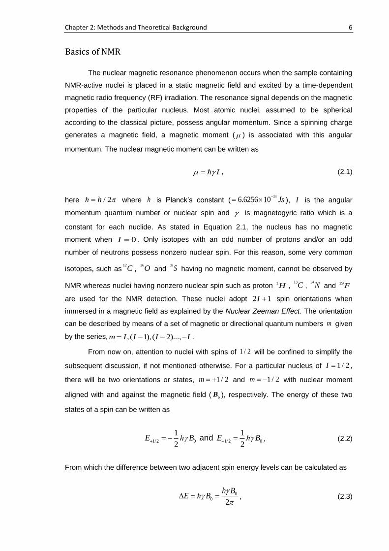
When a sample containing nuclei of 1 / 2I (e.g. 1H or
13C ) is placed in a
magnetic field (0
B ), each spin aligns in one of the two possible orientations as described
above. At thermal equilibrium, the number of spins in the lower and upper energy levels,
denoted by Nand N
, respectively, are not the same (figure 2.1 (a)).
This distribution of spins can be expressed using the Boltzmann statistics as given below
0/
1 1B B
BE k T BN E
k T k TNe
, (2.4)
where B
k is the Boltzmann constant (23 1
1.3805 10 JK
) and T is the temperature in
Kelvin. From the Equation 2.4, one can observe that the lower energy level is slightly
more populated than the higher energy level. This small difference in the number of
nuclei/spins is sufficient to allow an NMR signal to be detected which can be favored by a
stronger magnetic field (0
B ), a larger magnetogyric ratio ( ) and a lower temperature.
According to the classical picture, when placed in a magnetic field, the magnetic
moment of a spin precesses on a cone around the field axis z, keeping a constant angle
between the spin magnetic moment and the field. Since Nis greater than N
, the net
nuclear magnetization 0
M , which is the vector sum of the z-components of all the
individual nuclear magnetic moments in a sample, aligned parallel to the 0
B field direction
(figure 2.1 (b)). In this circumstance there is no transverse (x or y) magnetization (all x-y
components averages to zero). The characteristic angular frequency at which a magnetic
moment vector of a nuclei in a magnetic field precesses is called the Larmor frequency
( , in radians/second) which is given by
Figure 2.1: (a) Schematic drawing of the distribution of the nuclear dipoles in absence and in presence of the magnetic field. (b) Distribution of the nuclear dipoles gives rise to a net nuclear magnetization M0.
Chapter 2: Methods and Theoretical Background 8
0 B , (2.5)
This can be transformed into linear frequency ( Larmor , in Hertz or cycle/second) as
0
2 2L
B
, (2.6)
A combination of Equation 2.3 and 2.6 gives
LE h , (2.7)
If an electromagnetic radiation of frequency 1
is applied such a way that the resonance
condition 1 L
is fulfilled, then the transitions of the spins between the energy levels
can occur as the following Equation is satisfied
1E h , (2.8)
Absorption of energy occurs during the transition from the lower to the upper energy level
whereas those in the reverse direction correspond to an emission of energy. As described
before, the number of spins in the lower energy level is higher than the upper energy level
which leads to the absorption of energy from the irradiating field as the dominant process.
The intensity of the obtained signal (see below) is proportional to the difference of the
population of the spins which means that it is also proportional to the total number of spins
in the sample. When there is no difference in spin population between the two adjacent
energy levels, no signal is observed as the absorption and emission cancel each other
which is known as saturation.
The electromagnetic radiation in resonance with the Larmor frequency creates a
second magnetic field 1
B , which is applied to the sample along the direction of x-axis.
Because of this radiofrequency (RF) pulse, the net magnetization 0
M flips a certain angle
on a plane, perpendicular to the direction of 1
B . This gives rise to components of both
longitudinal and transverse magnetization relative to 0
B . The angle of tipping, is called
the pulse angle which is proportional to the magnetogyric ratio of the nuclei and to the
strength and duration of the pulse as given below
1 pB , (2.9)
Chapter 2: Methods and Theoretical Background 9
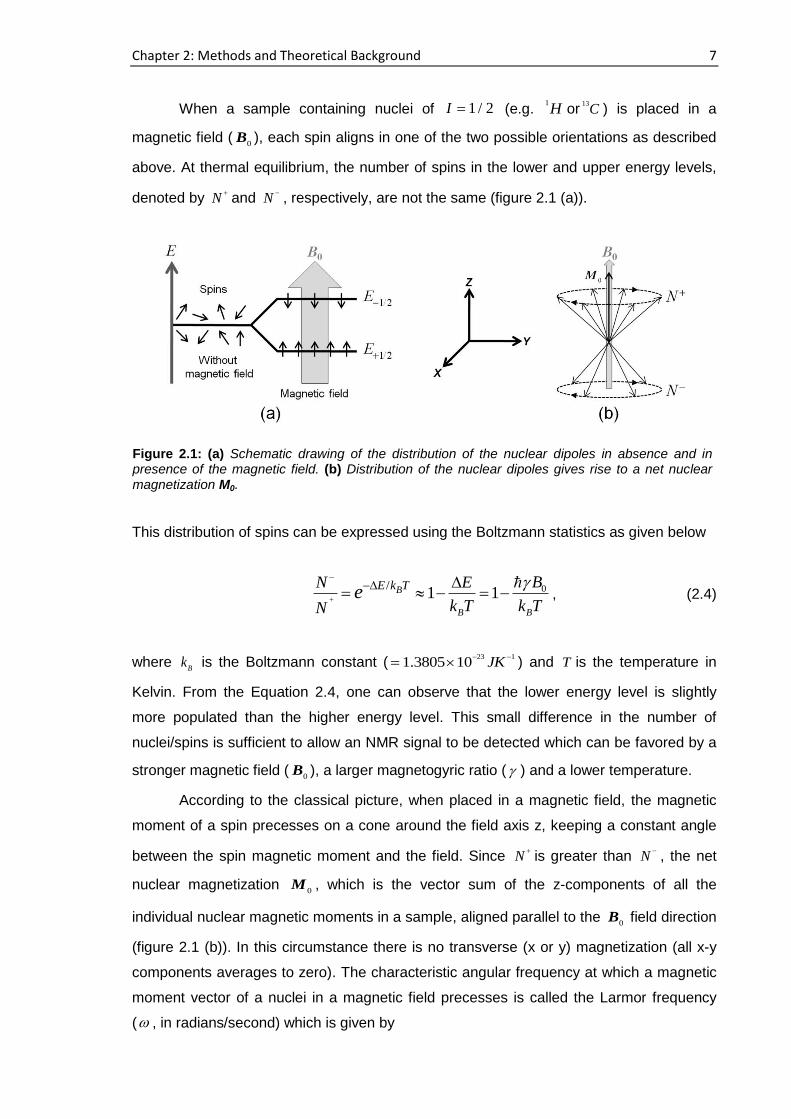
90° and 180° are the two major pulse angles that are used in the NMR experiments as
illustrated in figure 2.2. When the pulse is switched off, the net magnetization 0
M reverts
to its equilibrium state (parallel to the 0
B field direction) by the relaxation of the spins. This
process involves the discharge of the excess energy which is introduced in to the system
by the RF pulse.
In general, there are two types of relaxation process: longitudinal (or spin-lattice)
relaxation and transverse (or spin-spin) relaxation characterized by the constants 1
T and
2T , respectively. The decay of the transverse magnetization is known as free induction
decay (FID). The signal can be detected in the receiver as the induced voltage which is
/ dM dt , a consequence of precessing (transverse) magnetization. FID is a time
domain spectra. Fourier transformation (FT) is applied to the FID in order to observe the
spectra in the frequency domain.
Nuclear spin relaxation is caused by the distribution of local interactions
experienced by the nuclear spins. In general, the rotational relaxation and translational
displacement of nuclear spins influence the relaxation time. The relaxation is a
consequence of local fluctuating fields and it can be expressed via the FT of the
autocorrelation function of spin vectors.
Spin-lattice relaxation time
The recovery time at which the longitudinal component of the magnetization zM
comes into thermodynamic equilibrium is characterized by the spin-lattice relaxation time,
Figure 2.2: Graphical depiction of the flipping of the net nuclear magnetization M0 under the influence of radiofrequency pulse at resonance. (a) The net magnetization M0 is aligned along the external magnetic field B0 direction and the transverse magnetization component, Mxy is zero. (b) and (c) An RF filed B1 is applied perpendicular to B0 to tip the net magnetization by 90°. As a result, the longitudinal magnetization component, Mz becomes zero and the transverse magnetization component grows to its highest value. (d) After the 180°
pulse, the net
magnetization flips to –Z axis.

Chapter 2: Methods and Theoretical Background 10
1T (figure 2.3). The value of
1T covers a broad range depending on the nuclei type, the
location of the nuclei (i.e. atom) within a molecule, the size and the physical state of the
molecule and the temperature.
In this work, two common pulse sequences, namely, the saturation recovery and
the inversion recovery sequences are used to measure1
T . Two 90° pulses are used for
the saturation recovery sequence (figure 2.4 (a)) whereas an initial 180° pulse followed by
a 90° pulse is applied in the inversion recovery method (figure 2.4 (b)).
During the 1
T measurement, the delay time ( ) between two pulses, are varied and the
recovery of the corresponding longitudinal magnetizations is recorded. The magnetization
recovery can be expressed as
For the saturation recovery: 10
/( ) (1 )
z
TM M e
, (2.10)
For the inversion recovery: 1
0
/( ) (1 2 )
z
TM M e
, (2.11)
Figure 2.3: Graphical presentation of the recovery of the longitudinal magnetization, Mz. (a) After the 90°
pulse, Mz=0. (b) and (c) Recovery of Mz when the B1 field is switched off.
Figure 2.4: Pulse sequences for measuring T1 relaxation times using (a) Saturation recovery and (b) Inversion recovery sequences.
Chapter 2: Methods and Theoretical Background 11
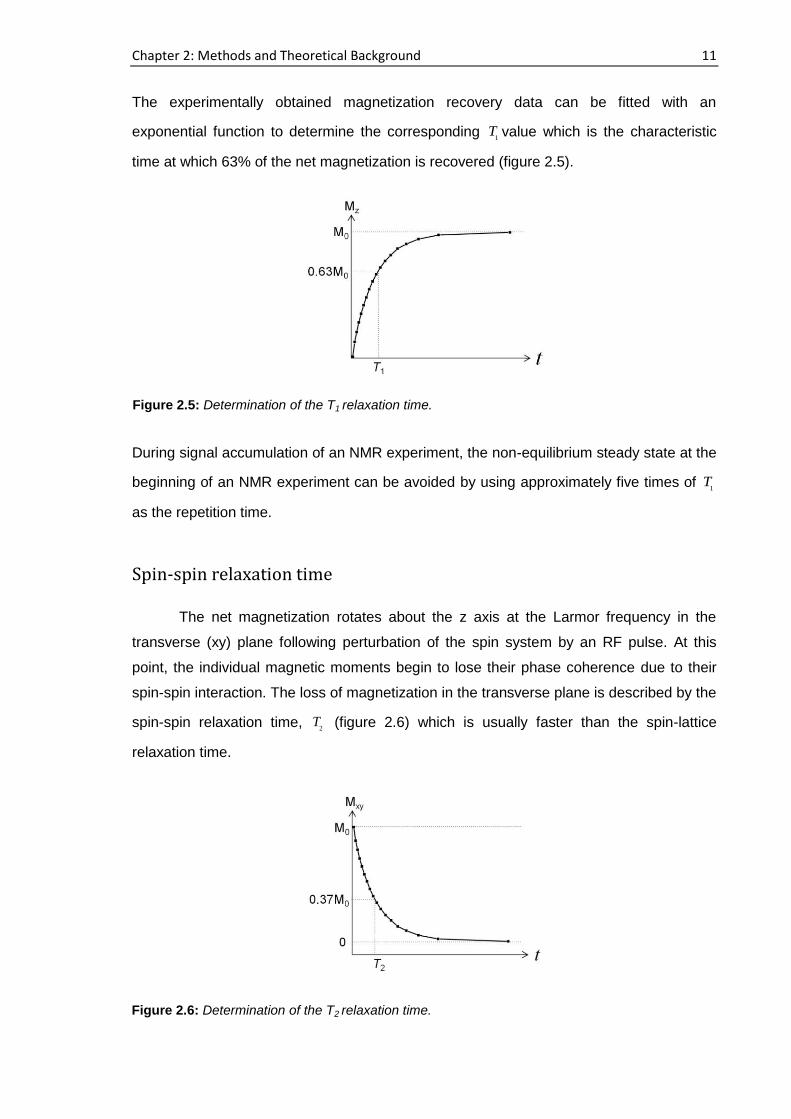
The experimentally obtained magnetization recovery data can be fitted with an
exponential function to determine the corresponding 1
T value which is the characteristic
time at which 63% of the net magnetization is recovered (figure 2.5).
During signal accumulation of an NMR experiment, the non-equilibrium steady state at the
beginning of an NMR experiment can be avoided by using approximately five times of 1
T
as the repetition time.
Spin-spin relaxation time
The net magnetization rotates about the z axis at the Larmor frequency in the
transverse (xy) plane following perturbation of the spin system by an RF pulse. At this
point, the individual magnetic moments begin to lose their phase coherence due to their
spin-spin interaction. The loss of magnetization in the transverse plane is described by the
spin-spin relaxation time, 2
T (figure 2.6) which is usually faster than the spin-lattice
relaxation time.
Figure 2.5: Determination of the T1 relaxation time.
Figure 2.6: Determination of the T2 relaxation time.
Chapter 2: Methods and Theoretical Background 12
2T can be expressed by
2/
0( )
t T
M t M e , (2.12)
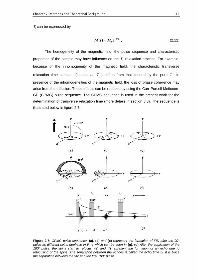
The homogeneity of the magnetic field, the pulse sequence and characteristic
properties of the sample may have influence on the 2
T relaxation process. For example,
because of the inhomogeneity of the magnetic field, the characteristic transverse
relaxation time constant (labeled as 2
T ) differs from that caused by the pure
2T . In
presence of the inhomogeneities of the magnetic field, the loss of phase coherence may
arise from the diffusion. These effects can be reduced by using the Carr-Purcell-Meiboom-
Gill (CPMG) pulse sequence. The CPMG sequence is used in the present work for the
determination of transverse relaxation time (more details in section 3.3). The sequence is
illustrated below in figure 2.7.
Figure 2.7: CPMG pulse sequence. (a), (b) and (c) represent the formation of FID after the 90°
pulse as different spins dephase in time which can be seen in (g). (d) After the application of the 180°
pulse, the spins start to refocus. (e) and (f) represent the formation of an echo due to
refocusing of the spins. The separation between the echoes is called the echo time tE. It is twice the separation between the 90°
and the first 180° pulse.
Chapter 2: Methods and Theoretical Background 13
In a strong inhomogeneous magnetic field, the characteristic relaxation time 2T
of
the FID might be very short. In the CPMG sequence, an initial 90° pulse is applied
followed by a series of 180° pulses. The successive echoes are formed in between each
of the 180° pulse pair and the decay of the amplitude of the direct echo will be dominated
by a longer characteristic time constant as can be seen in figure 2.7.
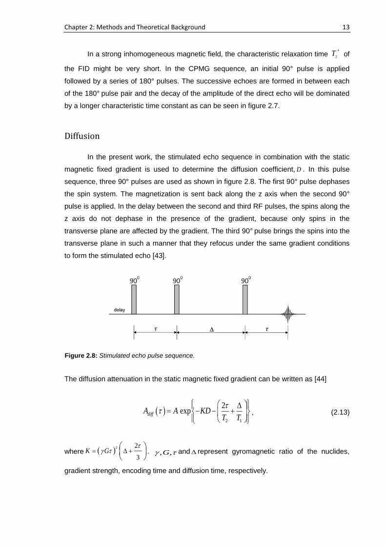
Diffusion
In the present work, the stimulated echo sequence in combination with the static
magnetic fixed gradient is used to determine the diffusion coefficient, D . In this pulse
sequence, three 90° pulses are used as shown in figure 2.8. The first 90° pulse dephases
the spin system. The magnetization is sent back along the z axis when the second 90°
pulse is applied. In the delay between the second and third RF pulses, the spins along the
z axis do not dephase in the presence of the gradient, because only spins in the
transverse plane are affected by the gradient. The third 90° pulse brings the spins into the
transverse plane in such a manner that they refocus under the same gradient conditions
to form the stimulated echo [43].
The diffusion attenuation in the static magnetic fixed gradient can be written as [44]
2 1
2exp
diffA A KD
T T
, (2.13)
where 2 2
3K G
. , ,G and represent gyromagnetic ratio of the nuclides,
gradient strength, encoding time and diffusion time, respectively.
Figure 2.8: Stimulated echo pulse sequence.
Chapter 2: Methods and Theoretical Background 14
2.2 X-ray Diffractometry (XRD)
The German Physicist Wilhelm Conrad Röntgen discovered X-rays in 1895. It is a
high-energy electromagnetic radiation having a wavelength from about 0.001 to 10 nm.
However, X-rays used to study the structure of the materials have a narrow range of
wavelengths of 0.05 to 0.25 nm. For the production of X-rays, electrons are generated by
heating a cathode (e.g., tungsten filament) in a vacuum chamber. These electrons are
accelerated towards an anode (e.g., copper) and collide with it at a very high velocity. If
the incident electron possesses sufficient energy to eject an inner-shell electron (having
lower average energy than that of outer-shell) from the atom of the anode metal, the atom
will be left in the excited stage. This inner-shell is filled by an electron from an outer-shell
of the atom and an X-ray photon is emitted as the atom returns to the ground state. When
an experimental set up is made such a way that the monochromatic X-ray beam hits a
sample, it generates scattered X-rays with the same wavelength as the incident beam.
The atomic arrangement of the sample is responsible for the intensities and spatial
distribution of the scattered X-rays. If the scattered waves are in phase, there is a
constructive interference which forms a spatial diffraction pattern in a specific direction.
These directions are governed by the wavelength ( ) of the incident beam and the
structure of the sample.
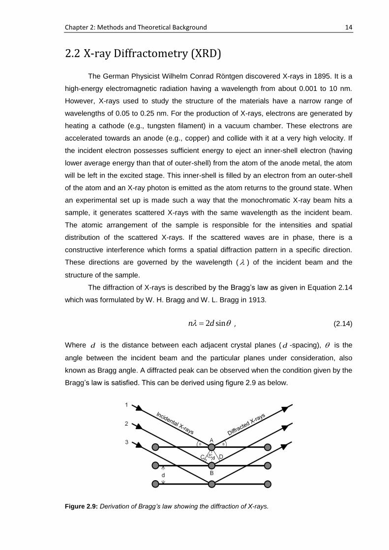
The diffraction of X-rays is described by the Bragg‟s law as given in Equation 2.14
which was formulated by W. H. Bragg and W. L. Bragg in 1913.
2 sin n d , (2.14)
Where d is the distance between each adjacent crystal planes ( d -spacing), is the
angle between the incident beam and the particular planes under consideration, also
known as Bragg angle. A diffracted peak can be observed when the condition given by the
Bragg‟s law is satisfied. This can be derived using figure 2.9 as below.
Figure 2.9: Derivation of Bragg’s law showing the diffraction of X-rays.
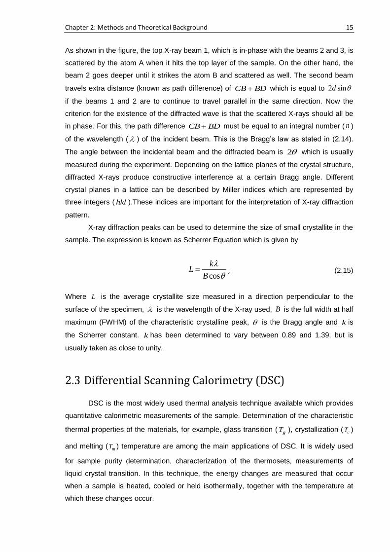
Chapter 2: Methods and Theoretical Background 15
As shown in the figure, the top X-ray beam 1, which is in-phase with the beams 2 and 3, is
scattered by the atom A when it hits the top layer of the sample. On the other hand, the
beam 2 goes deeper until it strikes the atom B and scattered as well. The second beam
travels extra distance (known as path difference) of CB BD which is equal to 2 sind
if the beams 1 and 2 are to continue to travel parallel in the same direction. Now the
criterion for the existence of the diffracted wave is that the scattered X-rays should all be
in phase. For this, the path difference CB BD must be equal to an integral number ( n )
of the wavelength ( ) of the incident beam. This is the Bragg‟s law as stated in (2.14).
The angle between the incidental beam and the diffracted beam is 2 which is usually
measured during the experiment. Depending on the lattice planes of the crystal structure,
diffracted X-rays produce constructive interference at a certain Bragg angle. Different
crystal planes in a lattice can be described by Miller indices which are represented by
three integers ( hkl ).These indices are important for the interpretation of X-ray diffraction
pattern.
X-ray diffraction peaks can be used to determine the size of small crystallite in the
sample. The expression is known as Scherrer Equation which is given by
cos
kL
B, (2.15)
Where L is the average crystallite size measured in a direction perpendicular to the
surface of the specimen, is the wavelength of the X-ray used, B is the full width at half
maximum (FWHM) of the characteristic crystalline peak, is the Bragg angle and k is
the Scherrer constant. k has been determined to vary between 0.89 and 1.39, but is
usually taken as close to unity.
2.3 Differential Scanning Calorimetry (DSC)
DSC is the most widely used thermal analysis technique available which provides
quantitative calorimetric measurements of the sample. Determination of the characteristic
thermal properties of the materials, for example, glass transition ( gT ), crystallization ( cT )
and melting ( mT ) temperature are among the main applications of DSC. It is widely used
for sample purity determination, characterization of the thermosets, measurements of
liquid crystal transition. In this technique, the energy changes are measured that occur
when a sample is heated, cooled or held isothermally, together with the temperature at
which these changes occur.
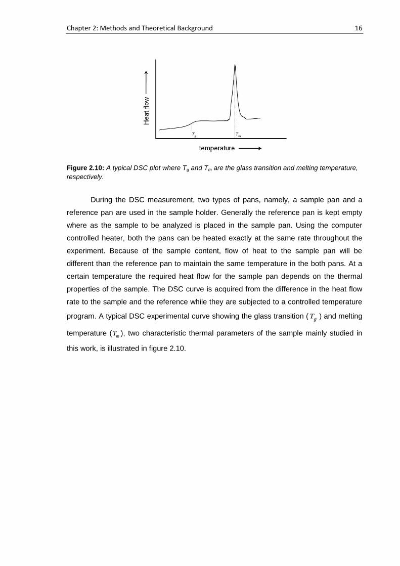
Chapter 2: Methods and Theoretical Background 16
During the DSC measurement, two types of pans, namely, a sample pan and a
reference pan are used in the sample holder. Generally the reference pan is kept empty
where as the sample to be analyzed is placed in the sample pan. Using the computer
controlled heater, both the pans can be heated exactly at the same rate throughout the
experiment. Because of the sample content, flow of heat to the sample pan will be
different than the reference pan to maintain the same temperature in the both pans. At a
certain temperature the required heat flow for the sample pan depends on the thermal
properties of the sample. The DSC curve is acquired from the difference in the heat flow
rate to the sample and the reference while they are subjected to a controlled temperature
program. A typical DSC experimental curve showing the glass transition ( gT ) and melting
temperature ( mT ), two characteristic thermal parameters of the sample mainly studied in
this work, is illustrated in figure 2.10.
Figure 2.10: A typical DSC plot where Tg and Tm are the glass transition and melting temperature,
respectively.
17
Chapter 3
Experimental
I didn’t think; I experimented.
Wilhelm Röntgen
This chapter consists of a short description of the polymer materials used in this
work (section 3.1), followed by the sample preparation techniques (section 3.2).
Afterwards, the single-sided NMR scanner, the low field NMR instrument mainly used to
study the polymer film formation and the data acquisition process are described in brief
along with the other NMR, XRD and DSC instruments which are used in this study
(section 3.3).
3.1. Materials
3.1.1. Introduction of the polymers
Gelatin
Gelatin is a water-soluble protein which is a hydrolyzed product of collagen. Similar
to the cellulose of plants, collagen is the abundant protein constituent in the animal
kingdom. The collagen structure consists of three distinct polypeptide chains, each twisted
in a left-handed helix ( chain) of about 0.9 nm pitch which are supercoiled together to
form a right-handed triple-helix with a pitch of about 8.6 nm. This triple-helix structure is
stabilized mainly by the intra and inter chain hydrogen bonding, close van der Waals
Chapter 3: Experimental 18
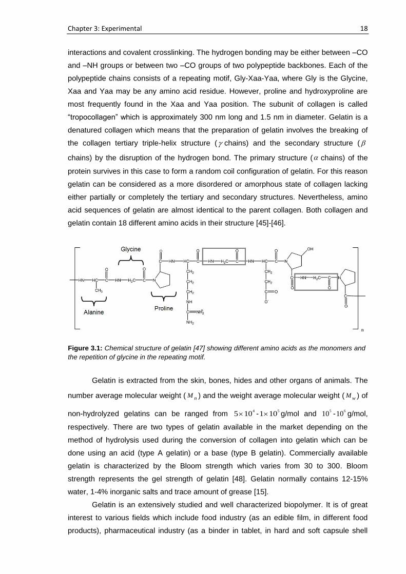
interactions and covalent crosslinking. The hydrogen bonding may be either between –CO
and –NH groups or between two –CO groups of two polypeptide backbones. Each of the
polypeptide chains consists of a repeating motif, Gly-Xaa-Yaa, where Gly is the Glycine,
Xaa and Yaa may be any amino acid residue. However, proline and hydroxyproline are
most frequently found in the Xaa and Yaa position. The subunit of collagen is called
“tropocollagen” which is approximately 300 nm long and 1.5 nm in diameter. Gelatin is a
denatured collagen which means that the preparation of gelatin involves the breaking of
the collagen tertiary triple-helix structure ( chains) and the secondary structure (
chains) by the disruption of the hydrogen bond. The primary structure ( chains) of the
protein survives in this case to form a random coil configuration of gelatin. For this reason
gelatin can be considered as a more disordered or amorphous state of collagen lacking
either partially or completely the tertiary and secondary structures. Nevertheless, amino
acid sequences of gelatin are almost identical to the parent collagen. Both collagen and
gelatin contain 18 different amino acids in their structure [45]-[46].
Gelatin is extracted from the skin, bones, hides and other organs of animals. The
number average molecular weight ( nM ) and the weight average molecular weight ( wM ) of
non-hydrolyzed gelatins can be ranged from 4
5 10 -5
1 10 g/mol and 5
10 -6
10 g/mol,
respectively. There are two types of gelatin available in the market depending on the
method of hydrolysis used during the conversion of collagen into gelatin which can be
done using an acid (type A gelatin) or a base (type B gelatin). Commercially available
gelatin is characterized by the Bloom strength which varies from 30 to 300. Bloom
strength represents the gel strength of gelatin [48]. Gelatin normally contains 12-15%
water, 1-4% inorganic salts and trace amount of grease [15].
Gelatin is an extensively studied and well characterized biopolymer. It is of great
interest to various fields which include food industry (as an edible film, in different food
products), pharmaceutical industry (as a binder in tablet, in hard and soft capsule shell
Figure 3.1: Chemical structure of gelatin [47] showing different amino acids as the monomers and
the repetition of glycine in the repeating motif.
Chapter 3: Experimental 19
production), biomedical field (for wound dressing, three-dimensional tissue regeneration,
adsorbent pads for surgical use, microspheres, sealants for vascular prostheses) and
leather industry (in tanning). The wide interest behind the increasing use of the gelatin film
is due, to a large degree, to its suitable mechanical properties combined with
biocompatibility, biodegradability and moisture sensitivity [4], [49]-[50].
Starch
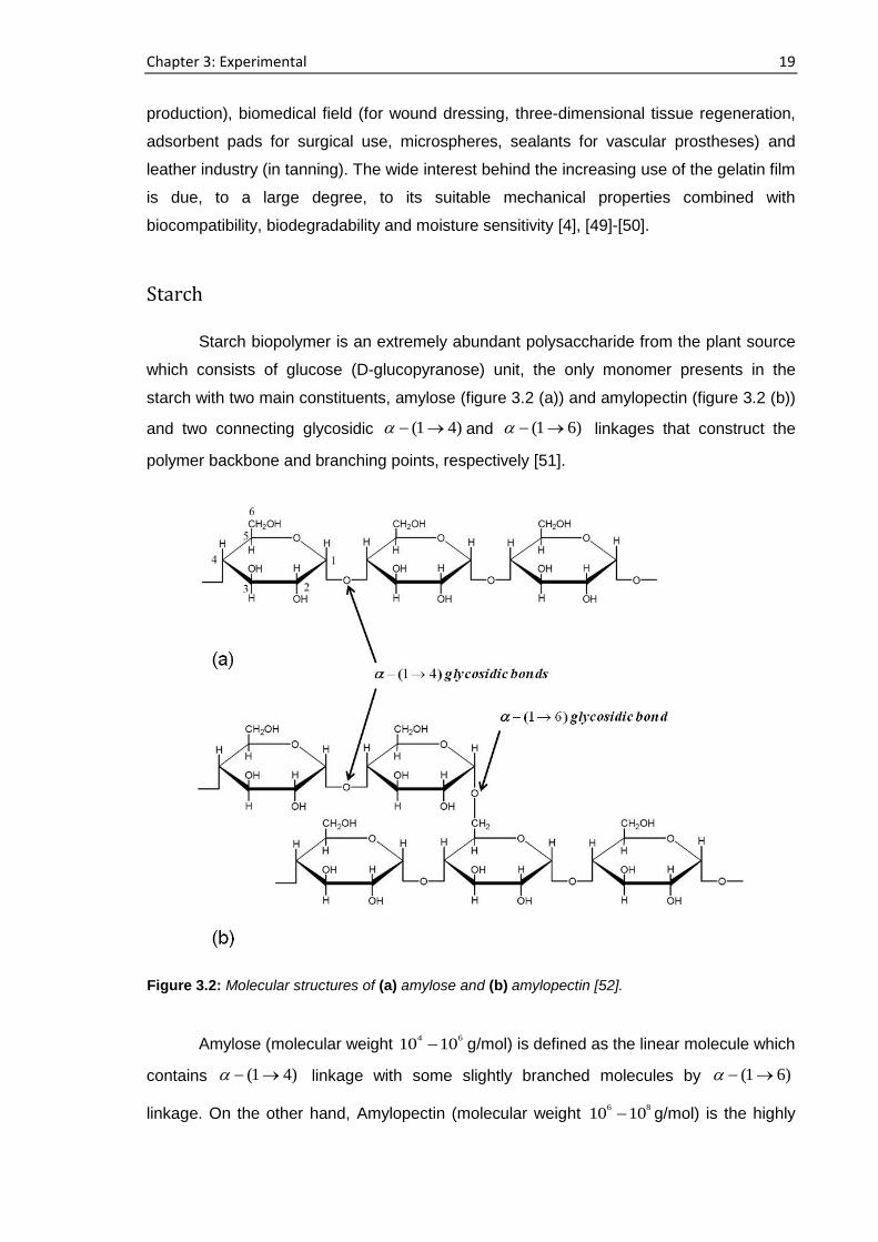
Starch biopolymer is an extremely abundant polysaccharide from the plant source
which consists of glucose (D-glucopyranose) unit, the only monomer presents in the
starch with two main constituents, amylose (figure 3.2 (a)) and amylopectin (figure 3.2 (b))
and two connecting glycosidic (1 4) and (1 6) linkages that construct the
polymer backbone and branching points, respectively [51].
Amylose (molecular weight 4 6
10 10 g/mol) is defined as the linear molecule which
contains (1 4) linkage with some slightly branched molecules by (1 6)
linkage. On the other hand, Amylopectin (molecular weight 6 8
10 10 g/mol) is the highly
Figure 3.2: Molecular structures of (a) amylose and (b) amylopectin [52].
Chapter 3: Experimental 20
branched component of starch which is composed mostly of (1 4) D-glucopyranose
units with (1 6) linkages at intervals of approximately 20 units [53].
Starch can be found in various parts of a plant, such as seeds, leaves, roots,
tubers and the fruit pulps. Based on plant origin or source, there are different kinds of
starch, for example, corn or maize starch, potato starch, rice starch, wheat starch etc. The
ratio of amylose to amylopectin in the starch granules varies with the plant source.
However, the amylose content in the commercially available starch granules is 20-30%.
There are some amylose-rich starches, for example, rice, wrinkled pea having amylose
content of over 50%. Proteins (up to 0.3%), minerals and lipids (up to 1.0%) are the other
components which are present in starch in very small quantities and have minor effect on
starch properties. Native starch granules have a crystallinity which varies from 12-45%
[16]. Amylopectin mainly forms the semi-crystalline zone in the starch granules which
consists of ordered double helical lamellar structure and rigid amorphous branching
zones. Some of the amylose may take part in this semi-crystalline zone by the formation
of double helices with amylopectin side chains [51], [54]. On the other hand, both amylose
and amylopectin contribute to the random ordered amorphous zone [55]. Depending on
the origin, the native starch has three crystalline patterns. For example, most cereal
starches have the so-called A-type pattern whereas B-type pattern appears in some tuber
and cereal starches rich in amylose. Legume starches generally give a C-type pattern. A-
type pattern has relatively more dense packed double helices than the B-type [16].
Application of starch film is steadily emerging, including biodegradable packaging
materials, as an alternative coating material in the food industry, barrier against gases (O2,
CO2), in the pharmaceutical industry as a carrier and so on [56]. Films prepared by the
starch are often very fragile. Hence, low molecular plasticizers such as polyols are used to
decrease interactions between the polymer chains [57]-[59]. The mechanical properties
such as tensile, bending and elongation properties of the film depend on starch source,
amylose-amylopectin ratios, moisture and plasticizer contents and film formation
parameters such as initial concentration, temperature, film formation time and relative
humidity.
Poly(vinyl alcohol) (PVOH)
There is a small number of synthetic polymers which are known for their
environment friendly behavior. Poly(vinyl alcohol) (PVOH), synthesized by Herrmann and
Haehnel in 1924, is one of those synthetic polymers which is biodegradable,
biocompatible and possesses good mechanical properties [60]. It is obtained from the
partial or complete hydrolysis of polyvinyl acetate. PVOH thermally degrades at about 150
Chapter 3: Experimental 21
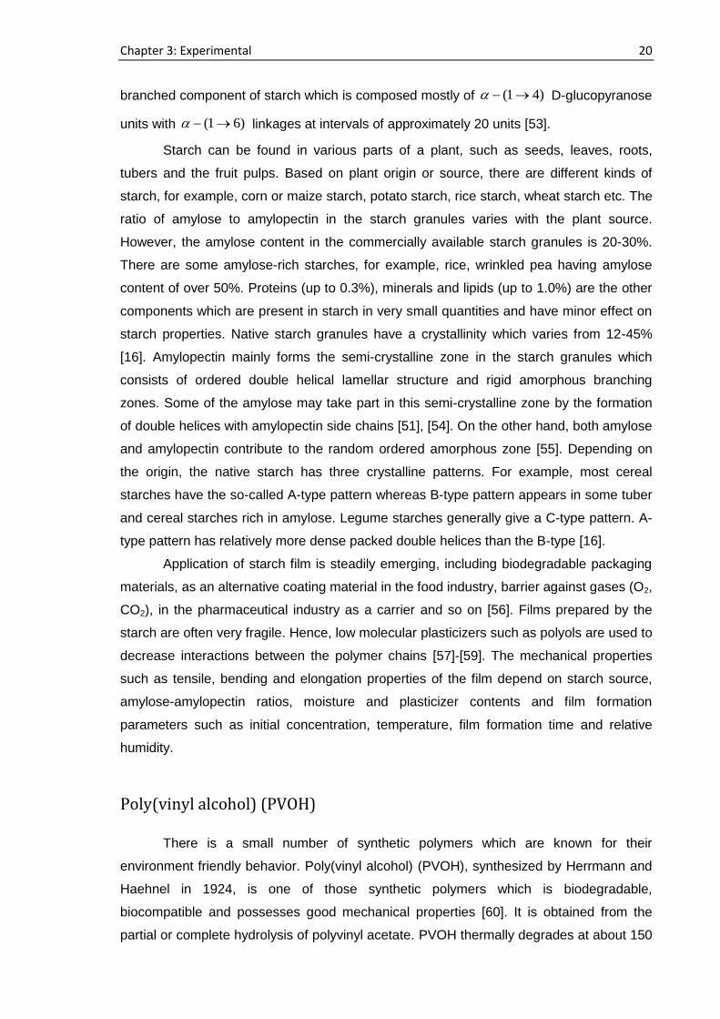
°C although the crystalline melting point is 180-240 °C [61]. Poly(vinyl alcohol) is a
tasteless, odorless hydrophilic polymer. In the solution it forms inter- and intramolecular
hydrogen bonds between –OH groups which is available in its monomer unit (figure 3.3).
Although PVOH is an atactic linear polymer which means the position of the –OH group in
the side chain is random, it is crystalline in nature as the small size of the –OH group does
not disrupt the crystalline lattice structure [17].
Commercially available PVOH has a broad range of hydrolysis and degree of
polymerizations which open the field of versatile applications in fibres, cosmetics industry,
adhesives, textile and paper sizing, asbestos alternatives, in pharmaceutical and
biomedical materials [62]-[64]. PVOH is a good film forming polymer which has
applications in different industrial sectors, for instance, as a high oxygen barrier film,
membranes, packaging materials and polarizing film as PVOH-iodine complex. It is also
readily blended with a number of natural materials, for example, gelatin, starch, chitosan
and alginate for new applications [65]-[67].
3.1.2. Materials used in this study
Gelatin
Gelatin from porcine skin containing 12-14% moisture (calculated from dry weight
basis) was used as received from Carl Roth GmbH + Co., Germany. It is an extra pure A
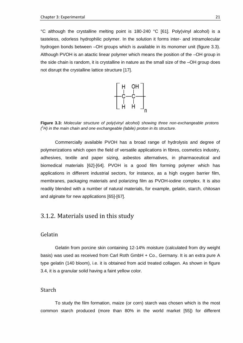
type gelatin (140 bloom), i.e. it is obtained from acid treated collagen. As shown in figure
3.4, it is a granular solid having a faint yellow color.
Starch
To study the film formation, maize (or corn) starch was chosen which is the most
common starch produced (more than 80% in the world market [55]) for different
Figure 3.3: Molecular structure of poly(vinyl alcohol) showing three non-exchangeable protons
(1H) in the main chain and one exchangeable (labile) proton in its structure.
Chapter 3: Experimental 22
applications. Unmodified extra pure corn starch (Carl Roth GmbH + Co.) containing 13%
moisture (dry weight basis) was used to follow the film formation in this work.
Poly(vinyl alcohol)
PVOH (MOWIOL grade) was obtained from Sigma-Aldrich, Germany and used
without further purification. Three different molecular weights of PVOH, 27000, 61000 and
125000 were used in this study with a degree of hydrolysis > 98% for all the samples. All
the samples contain around 15% of moisture which was calculated from dry weight basis.
Water (H2O)
In this study, water was used as the solvent of choice due to its ability to make
solution/suspension with the studied polymers. Mono distilled water was obtained from the
GFL-2002 water distillation unit (Gesellschaft für Labortechnik mbH, Germany) and used
to dissolve the polymer samples.
Deuterium oxide (D2O)
Deuterated water was used as a solvent in order to selectively follow the dynamics
of the backbone of the polymer molecules during the NMR experiments. D2O (100 atom-%
D) was purchased from Chemotrade, Chemiehandelsgesellschaft mbH, Leipzig, Germany
and Carl Roth GmbH + Co., Germany.
Glycerol
Anhydrous glycerol (Merk-Schuchardt, Germany) was used as a plasticizer. It is a
monosaccharide-based polyol which is widely used as a plasticizer due to its low
molecular weight in edible film applications. In the starch film, it is used to enhance the
flexibility and elasticity of the film as well as to prevent pore and crack formation [57].
Figure 3.4: Polymer samples (a) Gelatin (b) Starch (c) Poly(vinyl alcohol).
Chapter 3: Experimental 23
3.2. Methods
3.2.1. Sample preparation
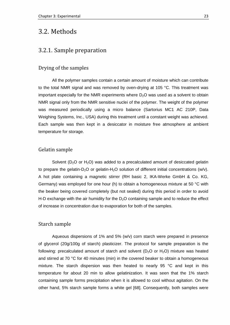
Drying of the samples
All the polymer samples contain a certain amount of moisture which can contribute
to the total NMR signal and was removed by oven-drying at 105 °C. This treatment was
important especially for the NMR experiments where D2O was used as a solvent to obtain
NMR signal only from the NMR sensitive nuclei of the polymer. The weight of the polymer
was measured periodically using a micro balance (Sartorius MC1 AC 210P, Data
Weighing Systems, Inc., USA) during this treatment until a constant weight was achieved.
Each sample was then kept in a desiccator in moisture free atmosphere at ambient
temperature for storage.
Gelatin sample
Solvent (D2O or H2O) was added to a precalculated amount of desiccated gelatin
to prepare the gelatin-D2O or gelatin-H2O solution of different initial concentrations (w/v).
A hot plate containing a magnetic stirrer (RH basic 2, IKA-Werke GmbH & Co. KG,
Germany) was employed for one hour (h) to obtain a homogeneous mixture at 50 °C with
the beaker being covered completely (but not sealed) during this period in order to avoid
H-D exchange with the air humidity for the D2O containing sample and to reduce the effect
of increase in concentration due to evaporation for both of the samples.
Starch sample
Aqueous dispersions of 1% and 5% (w/v) corn starch were prepared in presence
of glycerol (20g/100g of starch) plasticizer. The protocol for sample preparation is the
following: precalculated amount of starch and solvent (D2O or H2O) mixture was heated
and stirred at 70 °C for 40 minutes (min) in the covered beaker to obtain a homogeneous
mixture. The starch dispersion was then heated to nearly 95 °C and kept in this
temperature for about 20 min to allow gelatinization. It was seen that the 1% starch
containing sample forms precipitation when it is allowed to cool without agitation. On the
other hand, 5% starch sample forms a white gel [68]. Consequently, both samples were
Chapter 3: Experimental 24
agitated to maintain a homogeneous mixture until the sample temperature was reduced to
about 40 °C and cast afterwards.
Poly(vinyl alcohol) (PVOH) sample
For the preparation of the samples, either water or deuterium oxide was added to a
precalculated amount of desiccated PVOH to prepare the 25% (w/v) PVOH-H2O or 25%
(w/v) PVOH-D2O solutions, respectively. In order to obtain a homogeneous mixture and to
avoid local gelation, each of the PVOH samples was heated and stirred at 90 °C for one h,
with the beaker being covered completely during this period. Following this step, the
covered beaker containing the homogeneous mixture was placed in an oven and was kept
at the same temperature for further 5 h to eliminate air bubbles. The viscous solution was
then ready to cast.
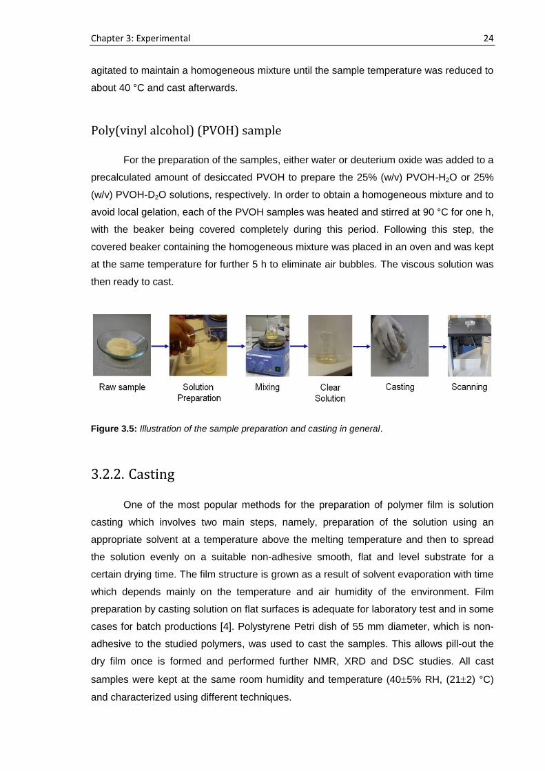
3.2.2. Casting
One of the most popular methods for the preparation of polymer film is solution
casting which involves two main steps, namely, preparation of the solution using an
appropriate solvent at a temperature above the melting temperature and then to spread
the solution evenly on a suitable non-adhesive smooth, flat and level substrate for a
certain drying time. The film structure is grown as a result of solvent evaporation with time
which depends mainly on the temperature and air humidity of the environment. Film
preparation by casting solution on flat surfaces is adequate for laboratory test and in some
cases for batch productions [4]. Polystyrene Petri dish of 55 mm diameter, which is non-
adhesive to the studied polymers, was used to cast the samples. This allows pill-out the
dry film once is formed and performed further NMR, XRD and DSC studies. All cast
samples were kept at the same room humidity and temperature (405% RH, (212) °C)
and characterized using different techniques.
Figure 3.5: Illustration of the sample preparation and casting in general.
Chapter 3: Experimental 25
3.3. Instrumentation
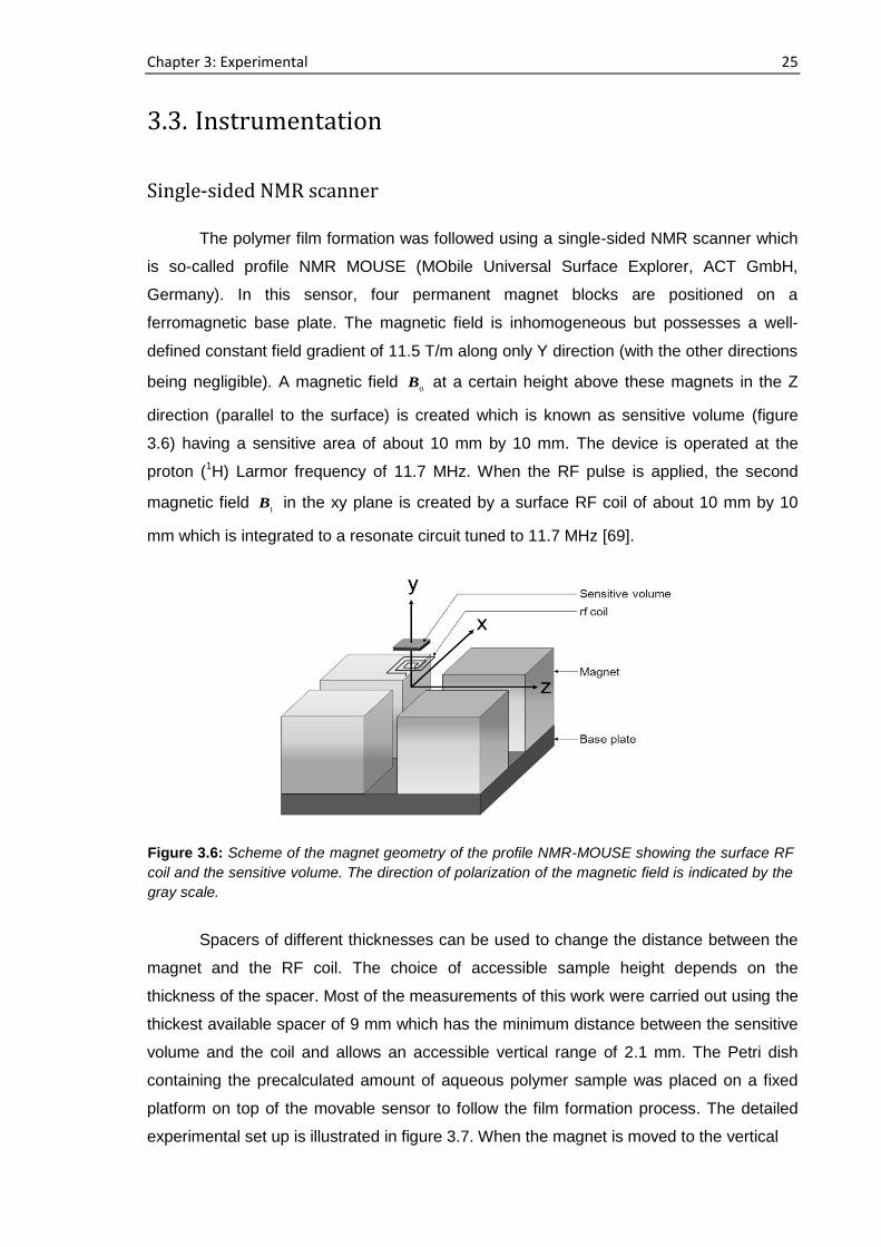
Single-sided NMR scanner
The polymer film formation was followed using a single-sided NMR scanner which
is so-called profile NMR MOUSE (MObile Universal Surface Explorer, ACT GmbH,
Germany). In this sensor, four permanent magnet blocks are positioned on a
ferromagnetic base plate. The magnetic field is inhomogeneous but possesses a well-
defined constant field gradient of 11.5 T/m along only Y direction (with the other directions
being negligible). A magnetic field 0
B at a certain height above these magnets in the Z
direction (parallel to the surface) is created which is known as sensitive volume (figure
3.6) having a sensitive area of about 10 mm by 10 mm. The device is operated at the
proton (1H) Larmor frequency of 11.7 MHz. When the RF pulse is applied, the second
magnetic field 1
B in the xy plane is created by a surface RF coil of about 10 mm by 10
mm which is integrated to a resonate circuit tuned to 11.7 MHz [69].
Spacers of different thicknesses can be used to change the distance between the
magnet and the RF coil. The choice of accessible sample height depends on the
thickness of the spacer. Most of the measurements of this work were carried out using the
thickest available spacer of 9 mm which has the minimum distance between the sensitive
volume and the coil and allows an accessible vertical range of 2.1 mm. The Petri dish
containing the precalculated amount of aqueous polymer sample was placed on a fixed
platform on top of the movable sensor to follow the film formation process. The detailed
experimental set up is illustrated in figure 3.7. When the magnet is moved to the vertical
Figure 3.6: Scheme of the magnet geometry of the profile NMR-MOUSE showing the surface RF
coil and the sensitive volume. The direction of polarization of the magnetic field is indicated by the
gray scale.
Chapter 3: Experimental 26
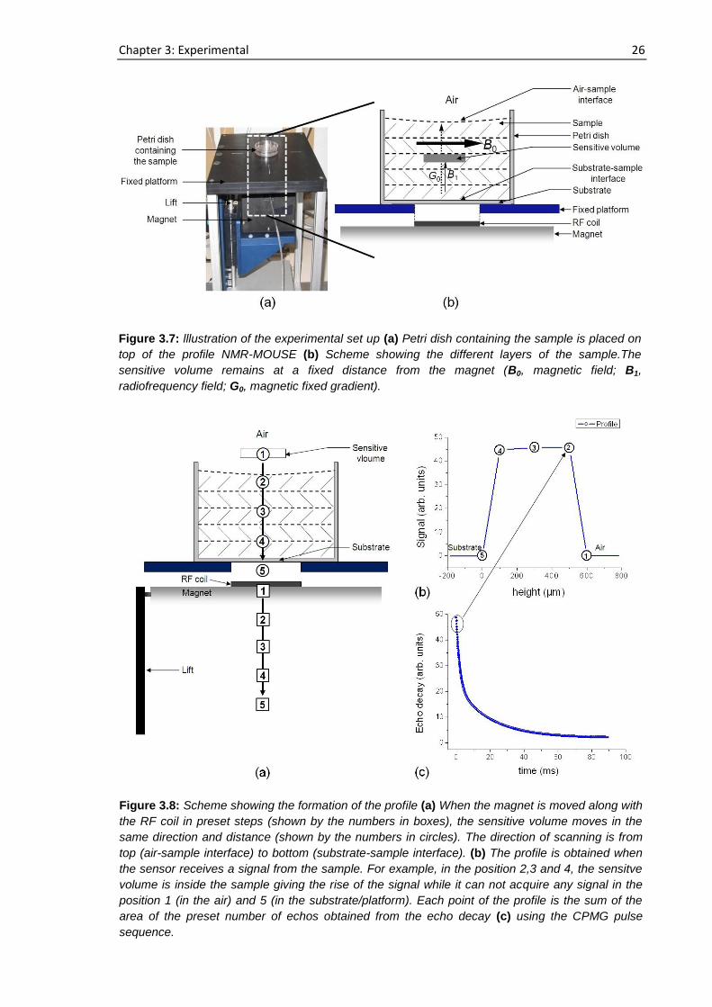
Figure 3.7: lllustration of the experimental set up (a) Petri dish containing the sample is placed on
top of the profile NMR-MOUSE (b) Scheme showing the different layers of the sample.The
sensitive volume remains at a fixed distance from the magnet (B0, magnetic field; B1,
radiofrequency field; G0, magnetic fixed gradient).
Figure 3.8: Scheme showing the formation of the profile (a) When the magnet is moved along with
the RF coil in preset steps (shown by the numbers in boxes), the sensitive volume moves in the
same direction and distance (shown by the numbers in circles). The direction of scanning is from
top (air-sample interface) to bottom (substrate-sample interface). (b) The profile is obtained when
the sensor receives a signal from the sample. For example, in the position 2,3 and 4, the sensitve
volume is inside the sample giving the rise of the signal while it can not acquire any signal in the
position 1 (in the air) and 5 (in the substrate/platform). Each point of the profile is the sum of the
area of the preset number of echos obtained from the echo decay (c) using the CPMG pulse
sequence.
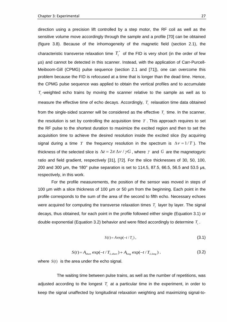
Chapter 3: Experimental 27
direction using a precision lift controlled by a step motor, the RF coil as well as the
sensitive volume move accordingly through the sample and a profile [70] can be obtained
(figure 3.8). Because of the inhomogeneity of the magnetic field (section 2.1), the
characteristic transverse relaxation time 2
T of the FID is very short (in the order of few
µs) and cannot be detected in this scanner. Instead, with the application of Carr-Purcell-
Meiboom-Gill (CPMG) pulse sequence (section 2.1 and [71]), one can overcome this
problem because the FID is refocused at a time that is longer than the dead time. Hence,
the CPMG pulse sequence was applied to obtain the vertical profiles and to accumulate
2T -weighted echo trains by moving the scanner relative to the sample as well as to
measure the effective time of echo decays. Accordingly, 2
T relaxation time data obtained
from the single-sided scanner will be considered as the effective 2
T time. In the scanner,
the resolution is set by controlling the acquisition time T . This approach requires to set
the RF pulse to the shortest duration to maximize the excited region and then to set the
acquisition time to achieve the desired resolution inside the excited slice (by acquiring
signal during a time T the frequency resolution in the spectrum is 1 / T ). The
thickness of the selected slice is 2 / z G , where and G are the magnetogyric
ratio and field gradient, respectively [31], [72]. For the slice thicknesses of 30, 50, 100,
200 and 300 μm, the 180° pulse separation is set to 114.5, 87.5, 66.5, 56.5 and 53.5 μs,
respectively, in this work.
For the profile measurements, the position of the sensor was moved in steps of
100 µm with a slice thickness of 100 µm or 50 µm from the beginning. Each point in the
profile corresponds to the sum of the area of the second to fifth echo. Necessary echoes
were acquired for computing the transverse relaxation times 2
T layer by layer. The signal
decays, thus obtained, for each point in the profile followed either single (Equation 3.1) or
double exponential (Equation 3.2) behavior and were fitted accordingly to determine 2
T .
2
( ) exp( / ) S t A t T , (3.1)
2, 2,( ) exp( / ) exp( / ) short short long longS t A t T A t T , (3.2)
where ( )S t is the area under the echo signal.
The waiting time between pulse trains, as well as the number of repetitions, was
adjusted according to the longest 1
T at a particular time in the experiment, in order to
keep the signal unaffected by longitudinal relaxation weighting and maximizing signal-to-
Chapter 3: Experimental 28
noise ratio for a given experimental run. This is due to the fact that the signal intensity is
proportional to [1
1 exp( / ) rep
t T ]. If the repetition time (rep
t ) is long enough, the 1
T -contrast
[73] is suppressed, and in consequence the signal intensity at different times of the drying
process is not affected. A saturation recovery pulse sequence [ 90 90 ] (section 2.1
and [74]) was used with 18 values (logarithmically spaced) and CPMG sequence for
acquisition [70] for determining the 1
T value. The number of steps for each profile was
reduced with drying time accordingly with the reduction of the thickness. This permits
more acquisition without increasing the time necessary to make a complete profile. 2
T
values of the fully dried films were also measured as a function of height using CPMG
pulse sequence in separate experiments. The 90° RF pulse length was set to 3.5 µs.
For the diffusion measurements, the stimulated echo sequence (section 2.1 and
[75]) in combination with the static magnetic gradient of the sensor was used. For this
measurement, if not mentioned otherwise, an encoding time = 0.0055 to 1.9 ms,
diffusion time = 2 ms, repetition time of 3 s to 5 s depending on the sample were used.
All experiments were performed at room temperature. The temperature of the magnet was
followed during the whole process, possessing a variation of ± 0.5 °C. At the position of
the sample, a minor increase in the temperature was detected due to the heating of the
RF coil. This heating was well below 0.5 °C.
Bruker minispec
The Minispec unit (Bruker Optics, Germany), a commercial low-field NMR
instrument operating at 40 MHz 1H Larmor frequency and equipped with a temperature
controller, was used to perform the proton relaxation measurements. This instrument
provides a simple tune-up system and a monotonically decaying on-resonance real FID
with negligible contributions in the imaginary part can be obtained with the proper
adjustment of the 90° pulse length, offset and receiver phase [76]. The samples were
measured using sealed 8 mm NMR tubes avoiding both evaporation and proton exchange
with the atmospheric humidity. To ensure sufficient magnetic field homogeneity, the
midpoint of the sample was adjusted to the center of the RF coil. All measurements were
carried out at (21.5 ± 0.5) °C. An inversion recovery pulse sequence [180 90 ]
(section 2.1 and [77], [78]) was used with 30 values (logarithmically spaced) to measure
the spin-lattice relaxation time (1
T ). The spin-spin relaxation time (2
T ) was obtained
applying the CPMG pulse sequence with a 90° - 180° pulse separation of 40 µs at a 180°
pulse width of 3.5 µs. The number of points, corresponding to number of echoes and the
number of scans were varied depending on the nature of the sample analyzed.

Chapter 3: Experimental 29
FIeld cycling relaxometer
The Stelar SPINMASTER FFC2000 relaxometer was used to obtain spin-lattice
relaxation times, 1
T over a wide range of Larmor frequency. The curves of 1
T in function of
frequency are called 1
T relaxation dispersion. In this method, the sample is polarized at a
polarization magnetic field pB for a time p (figure 3.9) enough for the nuclear
magnetization to reach the saturation. The relaxation process then takes place after the
fast switching 1 s to a lower magnetic field rB (relaxation field) in the interval time labeled
as r . At the end, the magnetic field is switched to a value of the higher acquisition field
aqB and the signal is acquired after a 90° RF pulse which has a frequency aqB . At a
certain magnetic field 1
T relaxation time is acquired by varying the time interval r . By this
way, 1
T relaxation dispersion is obtained by changing the field rB and measuring the
corresponding 1
T relaxation time [79].
The relaxation dispersions obtained in this study were measured in the interval
between 10 kHz and 20 MHz proton resonance frequency. All measurements were carried
out at (20.0 ± 0.5) °C.
X-ray diffractometer
The XRD patterns were acquired with a Philips X´Pert PRO diffractometer,
equipped with a wide-range PW 3050/6X goniometer which is capable to measure
Figure 3.9: Schematic representation of a typical cycle of the main magnetic field B0 employed
with field-cycling NMR relaxometry, where 1s and
2s represent the switching times to decrease
and increase the magnetic field, respectively.
Chapter 3: Experimental 30
0.001°/step. The calibration was carried out prior to each of the measurements and a
minimum offset for (incident angle) and 2 (diffraction angle) were achieved. The
experiment was carried out at room temperature using Cu K- radiation ( = 0.154 nm)
generated at a voltage of 35 kV and 30 mA current. The sample was scanned between
2 = 1.5 to 60° (for most of the samples) with a step size of 0.050°, scanning speed of 2°
/min and a count time of 100 s per point. Structural details of the polymer films were
examined by comparing the XRD pattern of both sides of the same film. The fixed angle
incident beam method was mainly used for this kind of experiments where = 0.5° was
fixed throughout the experiment. Powder diffraction spectra were collected as well to
characterize the raw polymer samples. Prior to the measurements, the sample was stored
in the same environmental conditions as employed for the NMR experiments.
Differential scanning calorimeter
Differential scanning calorimetry (DSC) curves of the polymer samples were
recorded with a DSC 7, TAC7/DX instrument (Perkin Elmer, USA) equipped with liquid
nitrogen cooling accessory. The transition temperature and enthalpy were calibrated using
indium standard. Each sample (5-8 mg) was accurately weighted into a 30 µl or 50 µl
standard aluminum pan containing the cover. The pan was perforated by a sealer. The
measurements were performed at different temperature ranges and rates as it will be
described in the corresponding sections.
Micro camera
A digital microscopic camera (Somikon, Pearl Agency Allgemeine
Vermittlungsgesellschaft mbH, Germany) was employed to capture real time frames at a
rate of 30 frames/h. In case of gelatin, a series of frames showing the reduction of the
sample height until the formation of film due to the solvent evaporation was processed
using a MATLAB routine. For the starch samples, still pictures were acquired at different
stages of film formation to visually compare different samples.
Other instruments
A Bruker MSL-300 Spectrometer at 300 MHz (1H Larmor frequency) and a Mettler
Toledo TGA/SDTA 851e thermogravimetric analyzer (TGA) were also used to study the
polymers at different stages of this work. More experimental details using these
instruments will be provided in the corresponding chapters.
31
Chapter 4
Study of gelatin film formation and its
characterization
Learn from yesterday, live for today, hope for tomorrow.
The important thing is not to stop questioning.
Albert Einstein
4.1. Introduction
Gelatin forms a solution consisting of flexible individual random coils in water.
When this solution is dried above the helix-coil transition temperature (~40 °C), the film
produced rarely contains any helix structure similar to the native collagen. On the other
hand, below the coil-helix transition temperature, the viscosity of this gelatin solution
gradually increases in time which results, even without evaporation, in a thermoreversible
transparent gel. The gelling of the gelatin solution results in the formation of three-
dimensional cross-linked networks through the development of triple-helix structure which
later can pack into fibrils similar to, but not as ordered as, the native tropocollagen fibrils
[80]. The gel becomes more structurally stable with time although it is not possible to
reach a permanent equilibrium phase due to the physical aging of the polymer. When the
gel is dried as a result of solvent evaporation, it becomes a rigid film that shows good
mechanical properties (the mechanical strength of gelatin film is comparable to some
synthetic polymers like polyethylene and polypropylene) and very little optical scattering
[81]. As the triple-helix content plays a vital role in the rigidity of the film, it is obvious that
the gelatin film prepared below the helix-coil transition temperature possesses different
thermo-mechanical properties than the film obtained from the higher temperature drying.
Chapter 4: Study of gelatin film formation and its characterization 32
The study of the physical gelation process has attracted considerable research
attention for many years [82]-[83]. It is known that the preparation conditions such as the
temperature and humidity during gelatin film formation are crucial. The mechanical
properties of this film depend also on those conditions and have been investigated in the
context of the water content [84], crystallinity and aging enthalpy [85]. Thermal properties
of different types of gelatin and their films have been reported in literature. From these
studies, it is evident that unbounded as well as the bound water present in the gelatin
determine their structural properties [86]. This can be investigated using NMR techniques
and a number of works has been reported in characterizing gelatin gels and films using
NMR spectroscopy [23]-[26]. All these studies however, give not much insight into the
mechanism of gelatin film formation process. In this work, the film formation of gelatin was
studied using a time-dependent low-field NMR 1D-microimaging (profile) measurement to
understand the gelatin-water system at molecular level starting from the different initial
concentrated solutions. By this way, a biopolymer film was traced during its formation
using an NMR experiment from the beginning until the end with microscopic resolution for
the first time (section 4.3.1). Furthermore, gelatin film formation was investigated using
high-field NMR spectrometer together with the differential scanning calorimetry (DSC)
using a different approach (section 4.3.2).
Another purpose of this work was to study the dried gelatin film using different
techniques like NMR, XRD and DSC (section 4.4). The results obtained from these
studies along with the results of gelatin film formation study are explained using a
proposed mechanism (section 4.5). In section 4.6, a study on gelatin film prepared varying
the initial concentration of gelatin in the solution is demonstrated at different relative
humidities.
4.2. Samples
Solutions starting from different initial concentrations of gelatin in water solvent
were prepared as described in section 3.2.1 and cast on the polystyrene Petri dishes at
room humidity and temperature (40% RH within 5%, (212) °C). Table 4.1 shows the
composition of the gelatin samples and the related studies. These samples were mainly
used to study the gelatin film formation and their characterization (section 4.3 and 4.4).
Beside these, a number of other samples were prepared which will be described in the
corresponding sections. The initial thickness of sample a, b and c were around 11, 8 and
1 mm, respectively. The thickness of sample a and b were more than the sample c which
were initially calculated (roughly) to obtain the final gelatin films of around 100 µm of
minimum thickness for the later characterization. An immediate gel formation of gelatin
Chapter 4: Study of gelatin film formation and its characterization 33
solutions was not observed for sample a, b, d and g because the solutions were not
concentrated. However, for sample c, e and f the relatively concentrated solution
immediately turned into a gel at room temperature, as is described for example in [80].
The final thickness of the films was measured using a digital micrometer (TOOLCRAFT
820918, Conrad Electronic GmbH, Germany).
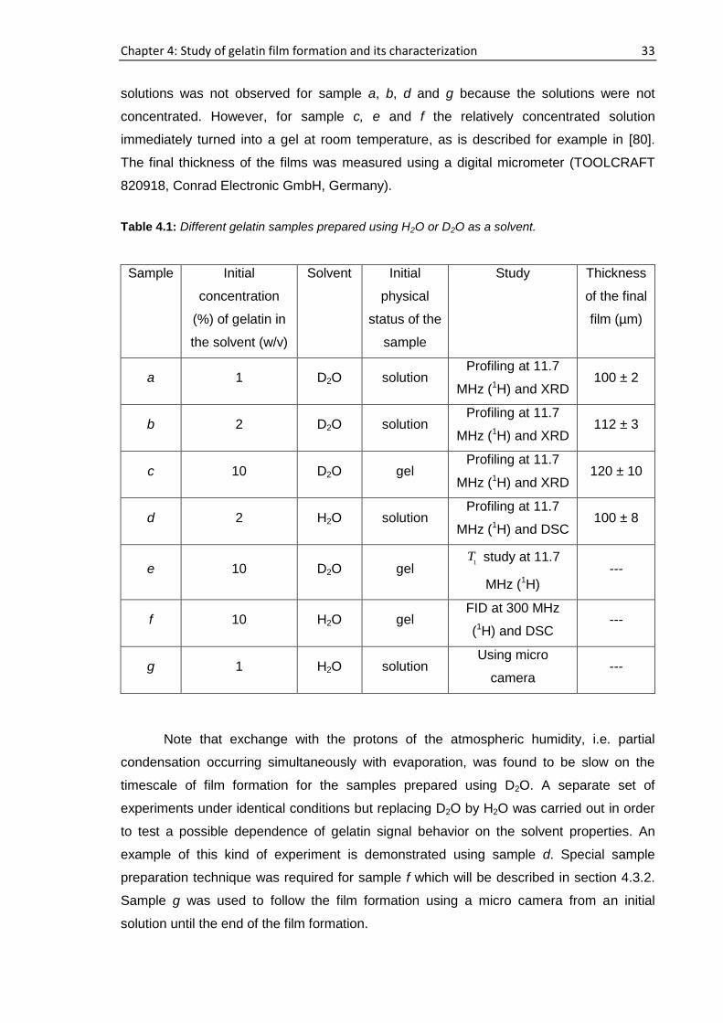
Table 4.1: Different gelatin samples prepared using H2O or D2O as a solvent.
Sample Initial
concentration
(%) of gelatin in
the solvent (w/v)
Solvent Initial
physical
status of the
sample
Study Thickness
of the final
film (µm)
a 1 D2O solution Profiling at 11.7
MHz (1H) and XRD 100 ± 2
b 2 D2O solution Profiling at 11.7
MHz (1H) and XRD 112 ± 3
c 10 D2O gel Profiling at 11.7
MHz (1H) and XRD 120 ± 10
d 2 H2O solution Profiling at 11.7
MHz (1H) and DSC 100 ± 8
e 10 D2O gel 1
T study at 11.7
MHz (1H) ---
f 10 H2O gel FID at 300 MHz
(1H) and DSC ---
g 1 H2O solution Using micro
camera ---
Note that exchange with the protons of the atmospheric humidity, i.e. partial
condensation occurring simultaneously with evaporation, was found to be slow on the
timescale of film formation for the samples prepared using D2O. A separate set of
experiments under identical conditions but replacing D2O by H2O was carried out in order
to test a possible dependence of gelatin signal behavior on the solvent properties. An
example of this kind of experiment is demonstrated using sample d. Special sample
preparation technique was required for sample f which will be described in section 4.3.2.
Sample g was used to follow the film formation using a micro camera from an initial
solution until the end of the film formation.
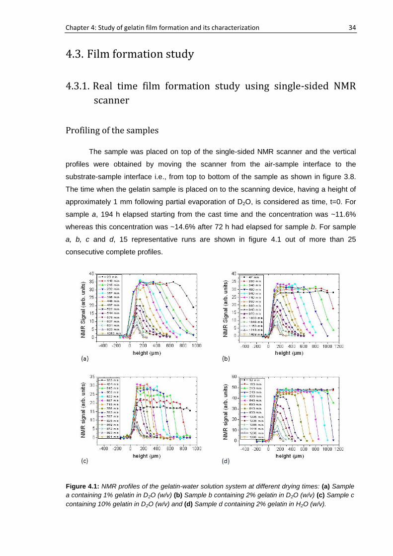
Chapter 4: Study of gelatin film formation and its characterization 34
4.3. Film formation study
4.3.1. Real time film formation study using single-sided NMR
scanner
Profiling of the samples
The sample was placed on top of the single-sided NMR scanner and the vertical
profiles were obtained by moving the scanner from the air-sample interface to the
substrate-sample interface i.e., from top to bottom of the sample as shown in figure 3.8.
The time when the gelatin sample is placed on to the scanning device, having a height of
approximately 1 mm following partial evaporation of D2O, is considered as time, t=0. For
sample a, 194 h elapsed starting from the cast time and the concentration was ~11.6%
whereas this concentration was ~14.6% after 72 h had elapsed for sample b. For sample
a, b, c and d, 15 representative runs are shown in figure 4.1 out of more than 25
consecutive complete profiles.
Figure 4.1: NMR profiles of the gelatin-water solution system at different drying times: (a) Sample
a containing 1% gelatin in D2O (w/v) (b) Sample b containing 2% gelatin in D2O (w/v) (c) Sample c
containing 10% gelatin in D2O (w/v) and (d) Sample d containing 2% gelatin in H2O (w/v).
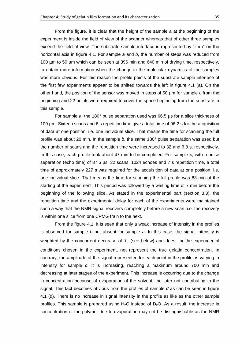
Chapter 4: Study of gelatin film formation and its characterization 35
From the figure, it is clear that the height of the sample a at the beginning of the
experiment is inside the field of view of the scanner whereas that of other three samples
exceed the field of view. The substrate-sample interface is represented by “zero” on the
horizontal axis in figure 4.1. For sample a and b, the number of steps was reduced from
100 µm to 50 µm which can be seen at 396 min and 640 min of drying time, respectively,
to obtain more information when the change in the molecular dynamics of the samples
was more obvious. For this reason the profile points of the substrate-sample interface of
the first few experiments appear to be shifted towards the left in figure 4.1 (a). On the
other hand, the position of the sensor was moved in steps of 50 µm for sample c from the
beginning and 22 points were required to cover the space beginning from the substrate in
this sample.
For sample a, the 180° pulse separation used was 66.5 µs for a slice thickness of
100 µm. Sixteen scans and 6 s repetition time give a total time of 96.2 s for the acquisition
of data at one position, i.e. one individual slice. That means the time for scanning the full
profile was about 20 min. In the sample b, the same 180° pulse separation was used but
the number of scans and the repetition time were increased to 32 and 6.8 s, respectively.
In this case, each profile took about 47 min to be completed. For sample c, with a pulse
separation (echo time) of 87.5 µs, 32 scans, 1024 echoes and 7 s repetition time, a total
time of approximately 227 s was required for the acquisition of data at one position, i.e.
one individual slice. That means the time for scanning the full profile was 83 min at the
starting of the experiment. This period was followed by a waiting time of 7 min before the
beginning of the following slice. As stated in the experimental part (section 3.3), the
repetition time and the experimental delay for each of the experiments were maintained
such a way that the NMR signal recovers completely before a new scan, i.e. the recovery
is within one slice from one CPMG train to the next.
From the figure 4.1, it is seen that only a weak increase of intensity in the profiles
is observed for sample b but absent for sample a. In this case, the signal intensity is
weighted by the concurrent decrease of 2
T (see below) and does, for the experimental
conditions chosen in the experiment, not represent the true gelatin concentration. In
contrary, the amplitude of the signal represented for each point in the profile, is varying in
intensity for sample c. It is increasing, reaching a maximum around 700 min and
decreasing at later stages of the experiment. This increase is occurring due to the change
in concentration because of evaporation of the solvent, the later not contributing to the
signal. This fact becomes obvious from the profiles of sample d as can be seen in figure
4.1 (d). There is no increase in signal intensity in the profile as like as the other sample
profiles. This sample is prepared using H2O instead of D2O. As a result, the increase in
concentration of the polymer due to evaporation may not be distinguishable as the NMR
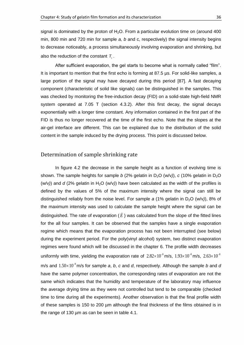
Chapter 4: Study of gelatin film formation and its characterization 36
signal is dominated by the proton of H2O. From a particular evolution time on (around 400
min, 800 min and 720 min for sample a, b and c, respectively) the signal intensity begins
to decrease noticeably, a process simultaneously involving evaporation and shrinking, but
also the reduction of the constant 2
T .
After sufficient evaporation, the gel starts to become what is normally called “film”.
It is important to mention that the first echo is forming at 87.5 µs. For solid-like samples, a
large portion of the signal may have decayed during this period [87]. A fast decaying
component (characteristic of solid like signals) can be distinguished in the samples. This
was checked by monitoring the free-induction decay (FID) on a solid-state high-field NMR
system operated at 7.05 T (section 4.3.2). After this first decay, the signal decays
exponentially with a longer time constant. Any information contained in the first part of the
FID is thus no longer recovered at the time of the first echo. Note that the slopes at the
air-gel interface are different. This can be explained due to the distribution of the solid
content in the sample induced by the drying process. This point is discussed below.
Determination of sample shrinking rate
In figure 4.2 the decrease in the sample height as a function of evolving time is
shown. The sample heights for sample b (2% gelatin in D2O (w/v)), c (10% gelatin in D2O
(w/v)) and d (2% gelatin in H2O (w/v)) have been calculated as the width of the profiles is
defined by the values of 5% of the maximum intensity where the signal can still be
distinguished reliably from the noise level. For sample a (1% gelatin in D2O (w/v)), 8% of
the maximum intensity was used to calculate the sample height where the signal can be
distinguished. The rate of evaporation ( E ) was calculated from the slope of the fitted lines
for the all four samples. It can be observed that the samples have a single evaporation
regime which means that the evaporation process has not been interrupted (see below)
during the experiment period. For the poly(vinyl alcohol) system, two distinct evaporation
regimes were found which will be discussed in the chapter 6. The profile width decreases
uniformly with time, yielding the evaporation rate of 8
2.82 10
m/s, 8
1.93 10
m/s, 8
2.63 10
m/s and 8
1.50 10
m/s for sample a, b, c and d, respectively. Although the sample b and d
have the same polymer concentration, the corresponding rates of evaporation are not the
same which indicates that the humidity and temperature of the laboratory may influence
the average drying time as they were not controlled but tend to be comparable (checked
time to time during all the experiments). Another observation is that the final profile width
of these samples is 150 to 200 µm although the final thickness of the films obtained is in
the range of 130 µm as can be seen in table 4.1.
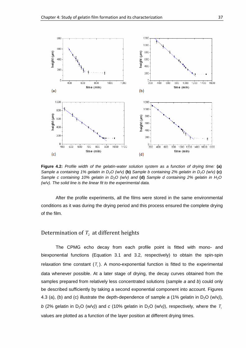
Chapter 4: Study of gelatin film formation and its characterization 37
After the profile experiments, all the films were stored in the same environmental
conditions as it was during the drying period and this process ensured the complete drying
of the film.
Determination of 2T at different heights
The CPMG echo decay from each profile point is fitted with mono- and
biexponential functions (Equation 3.1 and 3.2, respectively) to obtain the spin-spin
relaxation time constant (2
T ). A mono-exponential function is fitted to the experimental
data whenever possible. At a later stage of drying, the decay curves obtained from the
samples prepared from relatively less concentrated solutions (sample a and b) could only
be described sufficiently by taking a second exponential component into account. Figures
4.3 (a), (b) and (c) illustrate the depth-dependence of sample a (1% gelatin in D2O (w/v)),
b (2% gelatin in D2O (w/v)) and c (10% gelatin in D2O (w/v)), respectively, where the 2
T
values are plotted as a function of the layer position at different drying times.
Figure 4.2: Profile width of the gelatin-water solution system as a function of drying time: (a)
Sample a containing 1% gelatin in D2O (w/v) (b) Sample b containing 2% gelatin in D2O (w/v) (c)
Sample c containing 10% gelatin in D2O (w/v) and (d) Sample d containing 2% gelatin in H2O
(w/v). The solid line is the linear fit to the experimental data.
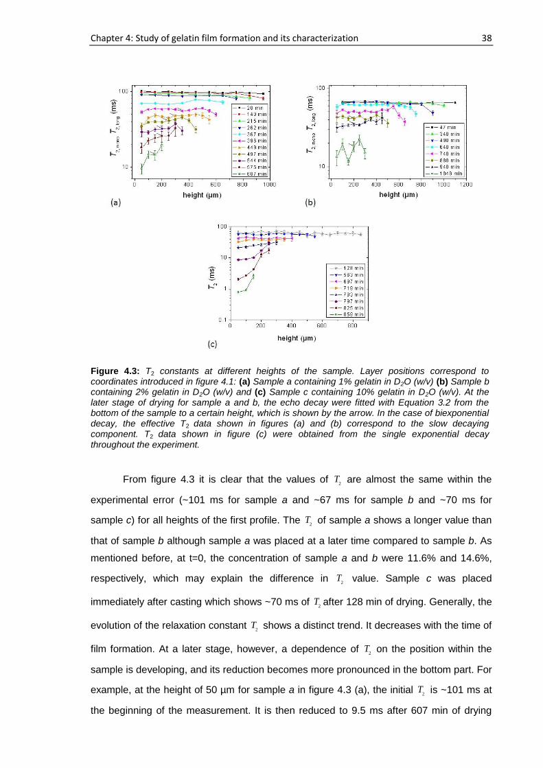
Chapter 4: Study of gelatin film formation and its characterization 38
From figure 4.3 it is clear that the values of 2
T are almost the same within the
experimental error (~101 ms for sample a and ~67 ms for sample b and ~70 ms for
sample c) for all heights of the first profile. The 2
T of sample a shows a longer value than
that of sample b although sample a was placed at a later time compared to sample b. As
mentioned before, at t=0, the concentration of sample a and b were 11.6% and 14.6%,
respectively, which may explain the difference in 2
T value. Sample c was placed
immediately after casting which shows ~70 ms of 2
T after 128 min of drying. Generally, the
evolution of the relaxation constant 2
T shows a distinct trend. It decreases with the time of
film formation. At a later stage, however, a dependence of 2
T on the position within the
sample is developing, and its reduction becomes more pronounced in the bottom part. For
example, at the height of 50 µm for sample a in figure 4.3 (a), the initial 2
T is ~101 ms at
the beginning of the measurement. It is then reduced to 9.5 ms after 607 min of drying
Figure 4.3: T2 constants at different heights of the sample. Layer positions correspond to coordinates introduced in figure 4.1: (a) Sample a containing 1% gelatin in D2O (w/v) (b) Sample b containing 2% gelatin in D2O (w/v) and (c) Sample c containing 10% gelatin in D2O (w/v). At the later stage of drying for sample a and b, the echo decay were fitted with Equation 3.2 from the bottom of the sample to a certain height, which is shown by the arrow. In the case of biexponential decay, the effective T2 data shown in figures (a) and (b) correspond to the slow decaying component. T2 data shown in figure (c) were obtained from the single exponential decay throughout the experiment.
Chapter 4: Study of gelatin film formation and its characterization 39
time. On the other hand, T2 reduces from ~100 ms to 19.2 ms during the same drying time
at the height of 200 µm. This effect is most prominent at the substrate-sample interface. A
close look at the 2
T values in figure 4.3 (a) up to ~500 min reveals that a similar, but less
pronounced, effect is observed at the top surface. For example, the 2
T value after 140 min
is ~96 ms at 450 µm which is reduced to ~81 ms at 950 µm height. The variation with
height in the vicinity of the air-sample interface is showing slightly more apparent effect in
figure 4.3 (b) up to 880 min. On the other hand, for sample c, the values of 2
T behave
almost the same at different layers, decreasing from ~68 ms to ~43 ms for all heights in
the first 697 min as can be seen in figure 4.3 (c). It means that the time scale of the
duration of the experiment is shorter than that of the characteristic time scale of the
process being studied, i.e. the formation of the film. After that, 2
T begins to vary from layer
to layer in the sample. From 719 min onwards, 2
T decreases sharply in the bottom part of
the sample. For example, in the bottom layer at 50 µm, initial value of 2
T is ~68 ms which
is decreased to ~800 µs after 859 min whereas it is reduced to ~2.5 ms at 150 µm height
starting from the same 2
T at 563 min. For this sample, no 2
T effect is observed at the top
surface as it was seen for sample a and b which means that the 2
T variation with height in
the vicinity of the air-sample interface can be observed only in the dilute sample.
In sample a, the echo decays show one component up to 367 min. From 396 min
of the measurement time the short component as well as a long component is detected
from the bottom of the sample up to 350 µm and one component is observed from 400 µm
to 600 µm. In sample b, short and long components are observed from 880 min onwards.
Hence, the 2
T values presented in figure 4.3 (a) and (b) are either the relaxation time of
the single component at an earlier stage or a combination of single and long component at
later stage. When the film is approaching the final drying stage, the 2
T of the film near the
substrate is significantly lower compared to the vicinity of the air-sample interface. For
sample b, this effect is less pronounced. Any effect here would be masked because of the
larger experimental error shown in the scatter of the data.
The dynamic heterogeneity of the sample can be seen directly from the raw echo
decays, for example, sample b as illustrated in figure 4.4. Here the echo decay for two
different layers, i.e. for 200 µm (from 47 to 970 min) and 400 µm (from 47 to 940 min) are
shown. From the figure, it becomes immediately obvious that the echo decays at 400 µm
remain monoexponential throughout the complete measurement period whereas the echo
decays at the height of 200 µm develop non-exponential behavior at later stages of drying.
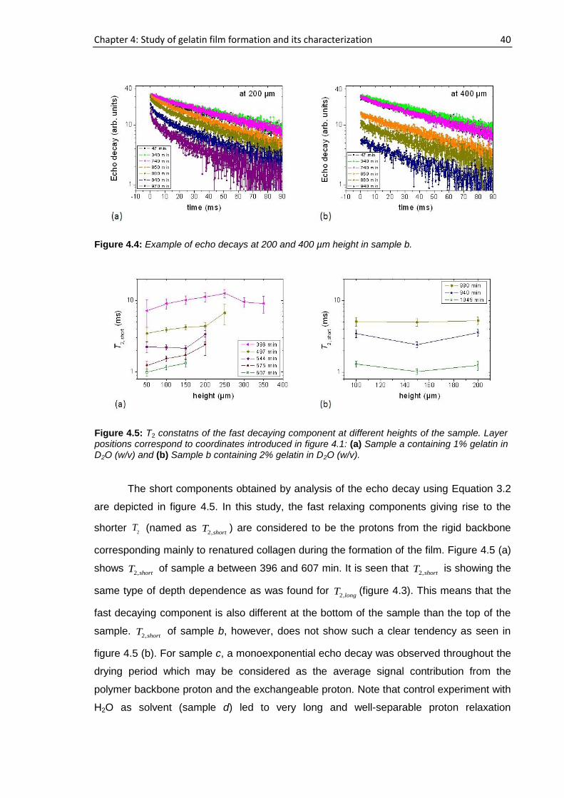
Chapter 4: Study of gelatin film formation and its characterization 40
The short components obtained by analysis of the echo decay using Equation 3.2
are depicted in figure 4.5. In this study, the fast relaxing components giving rise to the
shorter 2
T (named as 2,shortT ) are considered to be the protons from the rigid backbone
corresponding mainly to renatured collagen during the formation of the film. Figure 4.5 (a)
shows 2,shortT of sample a between 396 and 607 min. It is seen that
2,shortT is showing the
same type of depth dependence as was found for 2,longT (figure 4.3). This means that the
fast decaying component is also different at the bottom of the sample than the top of the
sample. 2,shortT of sample b, however, does not show such a clear tendency as seen in
figure 4.5 (b). For sample c, a monoexponential echo decay was observed throughout the
drying period which may be considered as the average signal contribution from the
polymer backbone proton and the exchangeable proton. Note that control experiment with
H2O as solvent (sample d) led to very long and well-separable proton relaxation
Figure 4.4: Example of echo decays at 200 and 400 µm height in sample b.
Figure 4.5: T2 constatns of the fast decaying component at different heights of the sample. Layer positions correspond to coordinates introduced in figure 4.1: (a) Sample a containing 1% gelatin in D2O (w/v) and (b) Sample b containing 2% gelatin in D2O (w/v).
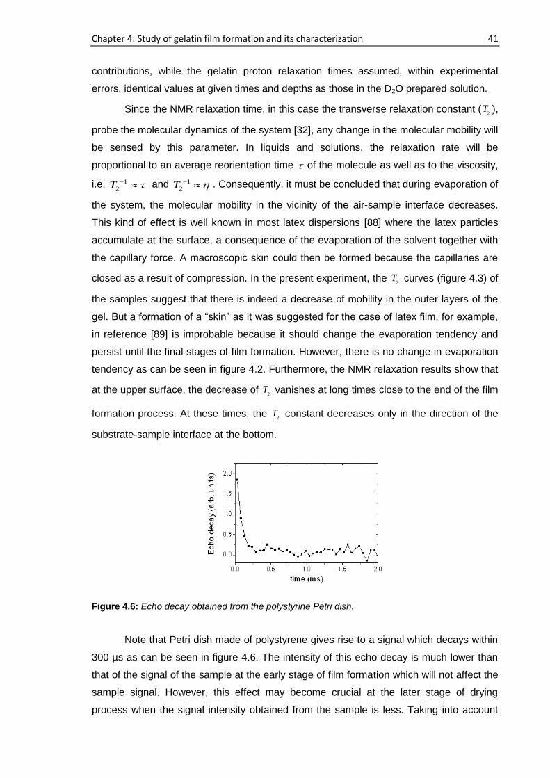
Chapter 4: Study of gelatin film formation and its characterization 41
contributions, while the gelatin proton relaxation times assumed, within experimental
errors, identical values at given times and depths as those in the D2O prepared solution.
Since the NMR relaxation time, in this case the transverse relaxation constant (2
T ),
probe the molecular dynamics of the system [32], any change in the molecular mobility will
be sensed by this parameter. In liquids and solutions, the relaxation rate will be
proportional to an average reorientation time of the molecule as well as to the viscosity,
i.e. 1
2 T and 1
2 T . Consequently, it must be concluded that during evaporation of
the system, the molecular mobility in the vicinity of the air-sample interface decreases.
This kind of effect is well known in most latex dispersions [88] where the latex particles
accumulate at the surface, a consequence of the evaporation of the solvent together with
the capillary force. A macroscopic skin could then be formed because the capillaries are
closed as a result of compression. In the present experiment, the 2
T curves (figure 4.3) of
the samples suggest that there is indeed a decrease of mobility in the outer layers of the
gel. But a formation of a “skin” as it was suggested for the case of latex film, for example,
in reference [89] is improbable because it should change the evaporation tendency and
persist until the final stages of film formation. However, there is no change in evaporation
tendency as can be seen in figure 4.2. Furthermore, the NMR relaxation results show that
at the upper surface, the decrease of 2
T vanishes at long times close to the end of the film
formation process. At these times, the 2
T constant decreases only in the direction of the
substrate-sample interface at the bottom.
Note that Petri dish made of polystyrene gives rise to a signal which decays within
300 µs as can be seen in figure 4.6. The intensity of this echo decay is much lower than
that of the signal of the sample at the early stage of film formation which will not affect the
sample signal. However, this effect may become crucial at the later stage of drying
process when the signal intensity obtained from the sample is less. Taking into account
Figure 4.6: Echo decay obtained from the polystyrine Petri dish.
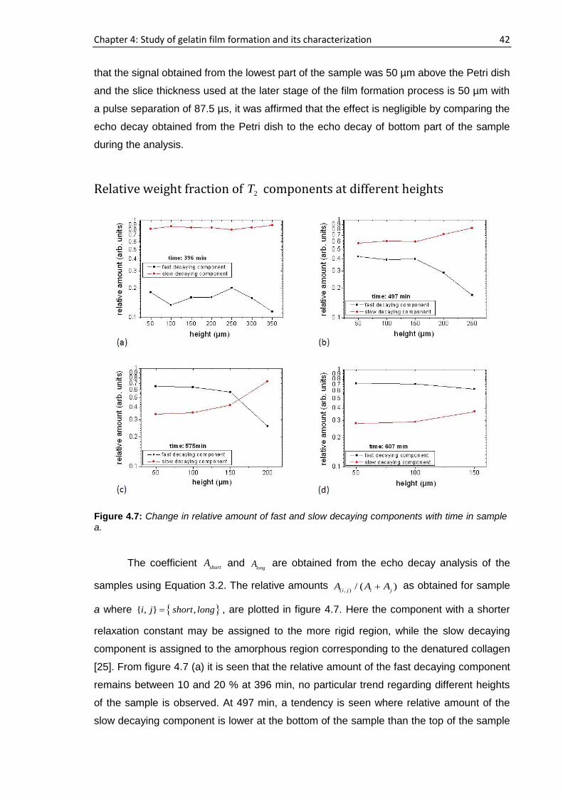
Chapter 4: Study of gelatin film formation and its characterization 42
that the signal obtained from the lowest part of the sample was 50 µm above the Petri dish
and the slice thickness used at the later stage of the film formation process is 50 µm with
a pulse separation of 87.5 µs, it was affirmed that the effect is negligible by comparing the
echo decay obtained from the Petri dish to the echo decay of bottom part of the sample
during the analysis.
Relative weight fraction of 2T components at different heights
The coefficient short
A and long
A are obtained from the echo decay analysis of the
samples using Equation 3.2. The relative amounts ( , )
/ ( )i j i j
A A A as obtained for sample
a where { , } ,i j short long , are plotted in figure 4.7. Here the component with a shorter
relaxation constant may be assigned to the more rigid region, while the slow decaying
component is assigned to the amorphous region corresponding to the denatured collagen
[25]. From figure 4.7 (a) it is seen that the relative amount of the fast decaying component
remains between 10 and 20 % at 396 min, no particular trend regarding different heights
of the sample is observed. At 497 min, a tendency is seen where relative amount of the
slow decaying component is lower at the bottom of the sample than the top of the sample
Figure 4.7: Change in relative amount of fast and slow decaying components with time in sample a.
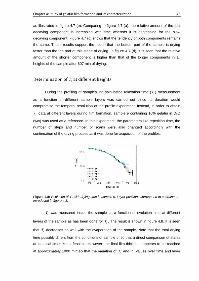
Chapter 4: Study of gelatin film formation and its characterization 43
as illustrated in figure 4.7 (b). Comparing to figure 4.7 (a), the relative amount of the fast
decaying component is increasing with time whereas it is decreasing for the slow
decaying component. Figure 4.7 (c) shows that the tendency of both components remains
the same. These results support the notion that the bottom part of the sample is drying
faster than the top part at this stage of drying. In figure 4.7 (d), it is seen that the relative
amount of the shorter component is higher than that of the longer components in all
heights of the sample after 607 min of drying.
Determination of 1T at different heights
During the profiling of samples, no spin-lattice relaxation time (1
T ) measurement
as a function of different sample layers was carried out since its duration would
compromise the temporal resolution of the profile experiment. Instead, in order to obtain
1T data at different layers during film formation, sample e containing 10% gelatin in D2O
(w/v) was used as a reference. In this experiment, the parameters like repetition time, the
number of steps and number of scans were also changed accordingly with the
continuation of the drying process as it was done for acquisition of the profiles.
1T was measured inside the sample as a function of evolution time at different
layers of the sample as has been done for 2
T . The result is shown in figure 4.8. It is seen
that 1
T decreases as well with the evaporation of the sample. Note that the total drying
time possibly differs from the conditions of sample c, so that a direct comparison of states
at identical times is not feasible. However, the final film thickness appears to be reached
at approximately 1000 min so that the variation of 2
T and 1
T values over time and layer
Figure 4.8: Evolution of T1 with drying time in sample e. Layer positions correspond to coordinates introduced in figure 4.1.
Chapter 4: Study of gelatin film formation and its characterization 44
thickness can be compared at least qualitatively. At the beginning, the maximum 1
T is
about 1700 ms. But after 200 min of drying, it begins to decrease significantly by more
than one order of magnitude. Considering different layers, there is no significant difference
in 1
T for times up to about 800 min. Then 1
T values start to vary between the layers. For
example, after 1025 min of drying, 1
T is 135 ms at 250 µm height but only 40 ms at the
height of 50 µm. This change in 1
T in different height of the sample confirms that the
drying of the gelatin film is inhomogeneous after a certain time period.
H-D Exchange
Because the system is prepared using D2O as a solvent, H-D exchange is
expected [90] but it is not introducing any systematic error in this experiment. Upon
dissolving gelatin in D2O, all exchangeable protons of the gelatin will exchange with D2O
molecules, thus producing a certain amount of HDO molecules. The relative fraction of
exchangeable protons can be estimated to about 15% [23], this results in a fraction of
approximate 0.25% of all deuterium oxide molecules to possess one proton; likewise,
99.75% of the exchangeable sites are now deuterated. Due to the fast exchange time
between the exchangeable protons and water (well below one second), this equilibrium is
maintained while D2O and HDO molecules are removed by evaporation (neglecting
different evaporation rates between these two). These HDO protons are responsible for
the long (about 6-7 seconds) component in T1 and mostly suppressed by the repetition
time, with the remaining contribution being a few % at most. This contribution is not
observed within the experimental error. Assuming fast exchange and the fact that the T2 of
protons in HDO is also several seconds, its influence on the measured 1H relaxation times
is negligible. The 1H distribution is expected to assume equilibrium in the early stages of
sample preparation. Only those approximate 15% of nuclei in exchangeable sites in the
gelatin may potentially be affected; the remainder does not exchange and manifests the
dominant signal contribution. It is this contribution that also undergoes the strong
reduction in T2, which can only be explained by a considerable reduction in mobility. The
limiting value of T2 ~300 µs (shown below in figure 4.14) suggests that a fraction of the
protons do not assume a rigid state but retain some degree of mobility.
The effect of exchange on the measured T2 value is minimized by the small
concentration of protons in the aqueous phase (HDO). Detailed studies, using pure H2O
and isotopic dilution, have been carried out by Hills et al [87] and suggest exchange rates
on the order of 2000 s-1. The echo times used in this study are shorter than the
Chapter 4: Study of gelatin film formation and its characterization 45
corresponding times and would lead to the measurement of the individual components of
T2 if they carried a sufficient signal contribution.
4.3.2. Gelatin film formation study using high-field NMR and
DSC
Renaturation process of gelatin at room temperature is of great interest to the
scientists for over 50 years [91]-[92]. Polarimetry, differential scanning calorimetry (DSC),
ultra-violet (UV) spectrometry, ultrasonic absorption, rheology and X-ray diffractometry
(XRD) are the common techniques which have been widely used to study the gelatin
renaturation. Flory and Weaver (1960) observed the renaturation of gelatin using
polarimetry and proposed a first order kinetics model of this process which had been the
most commonly accepted mechanism [93]. Later on, investigation of gelatin renaturation
mechanism has been carried out varying different parameters, for example, source of
gelatin, concentration of the solution and drying temperature [80], [94]-[96]. The focus of
these studies, in general, was to understand renaturation process of the gelatin keeping
the system in gel or solution state below the helix-coil transition temperature or from the
characterization of the final film. In this present study, gelatin film formation process was
followed using a combination of the high-field NMR spectroscopy and DSC methods while
the sample was under continuous evaporation and information on the renaturation
process for this kind of system was obtained.
A series of Petri dishes (35 mm diameter) was used to cast exactly the same
amount (by weight) of sample f (10% gelatin in H2O) in each Petri dish. All the Petri dishes
were placed in the same environmental conditions (40% RH within 5%, (192) °C) and let
them evolve. The samples immediately turned into a gel at room temperature. After
predetermined interval of time, one of the Petri dishes was collected for sample
preparation allowing the rest to further evolve. A required amount of gelatin sample was
prepared for NMR and DSC studies to measure immediately. It was assumed that the
evaporation tendency as well as the gel system would be disrupted due to the collection of
the sample from a Petri dish and it was not used further.
The initial amount of the gelatin sample was selected such a way that the drying
process continued for a long period and the required number of experiments was possible
to carried out to obtain sufficient data as a function of drying time. The optimized
experimental design also allowed conducting the successive NMR and DSC experiments
in each interval and repeating the experiments if necessary. It was found that the cast
sample became opaque at later stage (around 60 h) of evaporation although the
experiments were carried out until 100 h.
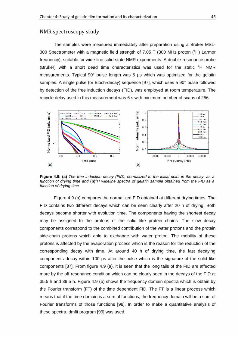
Chapter 4: Study of gelatin film formation and its characterization 46
NMR spectroscopy study
The samples were measured immediately after preparation using a Bruker MSL-
300 Spectrometer with a magnetic field strength of 7.05 T (300 MHz proton (1H) Larmor
frequency), suitable for wide-line solid-state NMR experiments. A double-resonance probe
(Bruker) with a short dead time characteristics was used for the static 1H NMR
measurements. Typical 90° pulse length was 5 µs which was optimized for the gelatin
samples. A single pulse (or Bloch-decay) sequence [97], which uses a 90° pulse followed
by detection of the free induction decays (FID), was employed at room temperature. The
recycle delay used in this measurement was 6 s with minimum number of scans of 256.
Figure 4.9 (a) compares the normalized FID obtained at different drying times. The
FID contains two different decays which can be seen clearly after 20 h of drying. Both
decays become shorter with evolution time. The components having the shortest decay
may be assigned to the protons of the solid like protein chains. The slow decay
components correspond to the combined contribution of the water protons and the protein
side-chain protons which able to exchange with water proton. The mobility of these
protons is affected by the evaporation process which is the reason for the reduction of the
corresponding decay with time. At around 40 h of drying time, the fast decaying
components decay within 100 µs after the pulse which is the signature of the solid like
components [87]. From figure 4.9 (a), it is seen that the long tails of the FID are affected
more by the off-resonance condition which can be clearly seen in the decays of the FID at
35.5 h and 39.5 h. Figure 4.9 (b) shows the frequency domain spectra which is obtain by
the Fourier transform (FT) of the time dependent FID. The FT is a linear process which
means that if the time domain is a sum of functions, the frequency domain will be a sum of
Fourier transforms of those functions [98]. In order to make a quantitative analysis of
these spectra, dmfit program [99] was used.
Figure 4.9: (a) The free induction decay (FID), normalized to the initial point in the decay, as a function of drying time and (b)
1H wideline spectra of gelatin sample obtained from the FID as a
function of drying time.
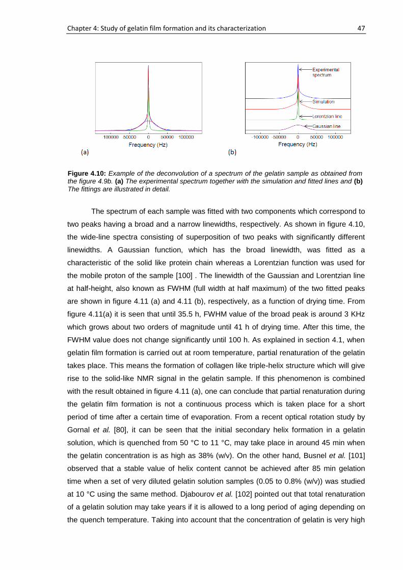
Chapter 4: Study of gelatin film formation and its characterization 47
The spectrum of each sample was fitted with two components which correspond to
two peaks having a broad and a narrow linewidths, respectively. As shown in figure 4.10,
the wide-line spectra consisting of superposition of two peaks with significantly different
linewidths. A Gaussian function, which has the broad linewidth, was fitted as a
characteristic of the solid like protein chain whereas a Lorentzian function was used for
the mobile proton of the sample [100] . The linewidth of the Gaussian and Lorentzian line
at half-height, also known as FWHM (full width at half maximum) of the two fitted peaks
are shown in figure 4.11 (a) and 4.11 (b), respectively, as a function of drying time. From
figure 4.11(a) it is seen that until 35.5 h, FWHM value of the broad peak is around 3 KHz
which grows about two orders of magnitude until 41 h of drying time. After this time, the
FWHM value does not change significantly until 100 h. As explained in section 4.1, when
gelatin film formation is carried out at room temperature, partial renaturation of the gelatin
takes place. This means the formation of collagen like triple-helix structure which will give
rise to the solid-like NMR signal in the gelatin sample. If this phenomenon is combined
with the result obtained in figure 4.11 (a), one can conclude that partial renaturation during
the gelatin film formation is not a continuous process which is taken place for a short
period of time after a certain time of evaporation. From a recent optical rotation study by
Gornal et al. [80], it can be seen that the initial secondary helix formation in a gelatin
solution, which is quenched from 50 °C to 11 °C, may take place in around 45 min when
the gelatin concentration is as high as 38% (w/v). On the other hand, Busnel et al. [101]
observed that a stable value of helix content cannot be achieved after 85 min gelation
time when a set of very diluted gelatin solution samples (0.05 to 0.8% (w/v)) was studied
at 10 °C using the same method. Djabourov et al. [102] pointed out that total renaturation
of a gelatin solution may take years if it is allowed to a long period of aging depending on
the quench temperature. Taking into account that the concentration of gelatin is very high
Figure 4.10: Example of the deconvolution of a spectrum of the gelatin sample as obtained from the figure 4.9b. (a) The experimental spectrum together with the simulation and fitted lines and (b) The fittings are illustrated in detail.
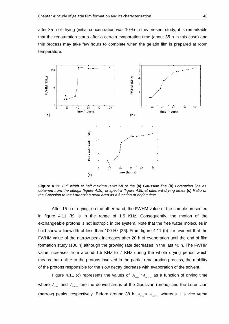
Chapter 4: Study of gelatin film formation and its characterization 48
after 35 h of drying (initial concentration was 10%) in this present study, it is remarkable
that the renaturation starts after a certain evaporation time (about 35 h in this case) and
this process may take few hours to complete when the gelatin film is prepared at room
temperature.
After 15 h of drying, on the other hand, the FWHM value of the sample presented
in figure 4.11 (b) is in the range of 1.5 KHz. Consequently, the motion of the
exchangeable protons is not isotropic in the system. Note that the free water molecules in
fluid show a linewidth of less than 100 Hz [26]. From figure 4.11 (b) it is evident that the
FWHM value of the narrow peak increases after 20 h of evaporation until the end of film
formation study (100 h) although the growing rate decreases in the last 40 h. The FWHM
value increases from around 1.5 KHz to 7 KHz during the whole drying period which
means that unlike to the protons involved in the partial renaturation process, the mobility
of the protons responsible for the slow decay decrease with evaporation of the solvent.
Figure 4.11 (c) represents the values of /broad narrow
A A as a function of drying time
where broad
A and
narrowA
are the derived areas of the Gaussian (broad) and the Lorentzian
(narrow) peaks, respectively. Before around 38 h, broad
A < narrow
A whereas it is vice versa
Figure 4.11: Full width at half maxima (FWHM) of the (a) Gaussian line (b) Lorentzian line as obtained from the fittings (figure 4.10) of spectra (figure 4.9b)at different drying times (c) Ratio of the Gaussian to the Lorentzian peak area as a function of drying time.
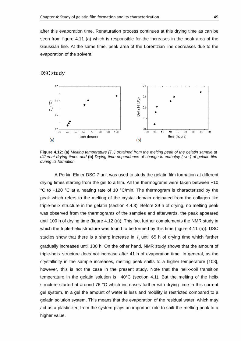
Chapter 4: Study of gelatin film formation and its characterization 49
Figure 4.12: (a) Melting temperature (Tm) obtained from the melting peak of the gelatin sample at different drying times and (b) Drying time dependence of change in enthalpy ( H ) of gelatin film during its formation.
after this evaporation time. Renaturation process continues at this drying time as can be
seen from figure 4.11 (a) which is responsible for the increases in the peak area of the
Gaussian line. At the same time, peak area of the Lorentzian line decreases due to the
evaporation of the solvent.
DSC study
A Perkin Elmer DSC 7 unit was used to study the gelatin film formation at different
drying times starting from the gel to a film. All the thermograms were taken between +10
°C to +120 °C at a heating rate of 10 °C/min. The thermogram is characterized by the
peak which refers to the melting of the crystal domain originated from the collagen like
triple-helix structure in the gelatin (section 4.4.3). Before 39 h of drying, no melting peak
was observed from the thermograms of the samples and afterwards, the peak appeared
until 100 h of drying time (figure 4.12 (a)). This fact further complements the NMR study in
which the triple-helix structure was found to be formed by this time (figure 4.11 (a)). DSC
studies show that there is a sharp increase in m
T until 65 h of drying time which further
gradually increases until 100 h. On the other hand, NMR study shows that the amount of
triple-helix structure does not increase after 41 h of evaporation time. In general, as the
crystallinity in the sample increases, melting peak shifts to a higher temperature [103],
however, this is not the case in the present study. Note that the helix-coil transition
temperature in the gelatin solution is ~40°C (section 4.1). But the melting of the helix
structure started at around 76 °C which increases further with drying time in this current
gel system. In a gel the amount of water is less and mobility is restricted compared to a
gelatin solution system. This means that the evaporation of the residual water, which may
act as a plasticizer, from the system plays an important role to shift the melting peak to a
higher value.
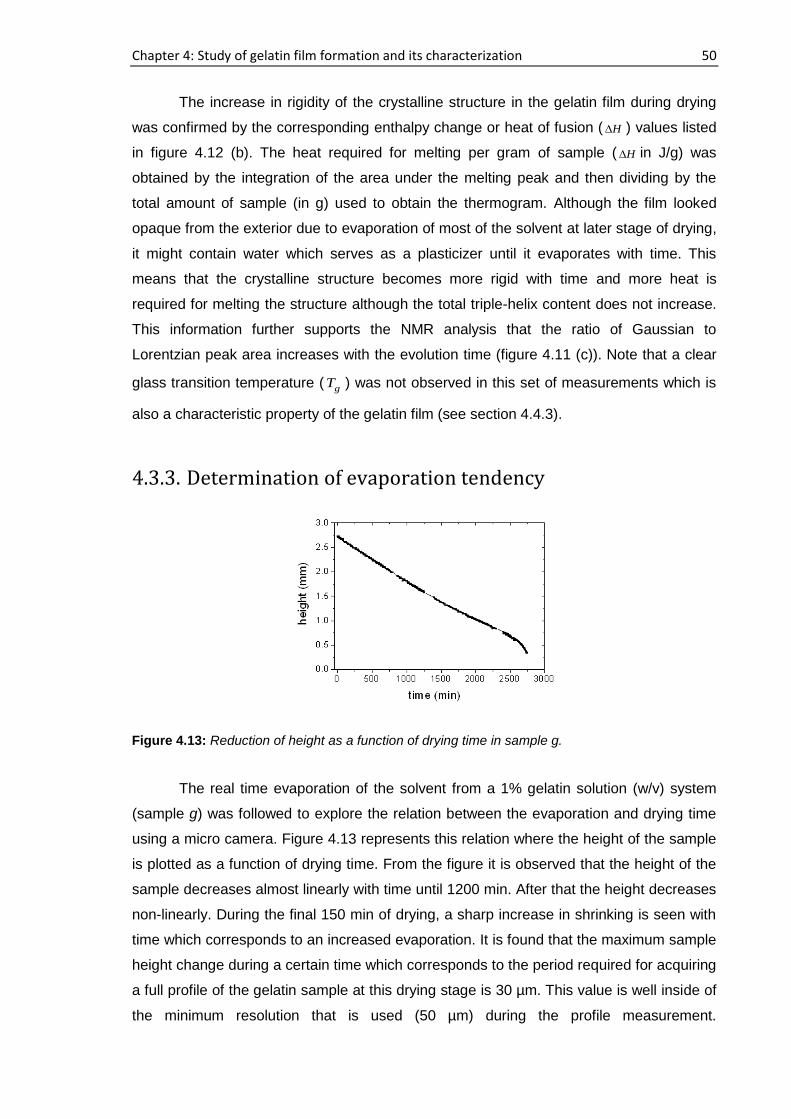
Chapter 4: Study of gelatin film formation and its characterization 50
The increase in rigidity of the crystalline structure in the gelatin film during drying
was confirmed by the corresponding enthalpy change or heat of fusion ( H ) values listed
in figure 4.12 (b). The heat required for melting per gram of sample ( H in J/g) was
obtained by the integration of the area under the melting peak and then dividing by the
total amount of sample (in g) used to obtain the thermogram. Although the film looked
opaque from the exterior due to evaporation of most of the solvent at later stage of drying,
it might contain water which serves as a plasticizer until it evaporates with time. This
means that the crystalline structure becomes more rigid with time and more heat is
required for melting the structure although the total triple-helix content does not increase.
This information further supports the NMR analysis that the ratio of Gaussian to
Lorentzian peak area increases with the evolution time (figure 4.11 (c)). Note that a clear
glass transition temperature ( gT ) was not observed in this set of measurements which is
also a characteristic property of the gelatin film (see section 4.4.3).
4.3.3. Determination of evaporation tendency
The real time evaporation of the solvent from a 1% gelatin solution (w/v) system
(sample g) was followed to explore the relation between the evaporation and drying time
using a micro camera. Figure 4.13 represents this relation where the height of the sample
is plotted as a function of drying time. From the figure it is observed that the height of the
sample decreases almost linearly with time until 1200 min. After that the height decreases
non-linearly. During the final 150 min of drying, a sharp increase in shrinking is seen with
time which corresponds to an increased evaporation. It is found that the maximum sample
height change during a certain time which corresponds to the period required for acquiring
a full profile of the gelatin sample at this drying stage is 30 µm. This value is well inside of
the minimum resolution that is used (50 µm) during the profile measurement.
Figure 4.13: Reduction of height as a function of drying time in sample g.

Chapter 4: Study of gelatin film formation and its characterization 51
Consequently, this quick shrinkage would not affect the phenomenon which is seen in the
present study. Note that this effect is absent in figure 4.2 where the evaporation tendency
is determined from the width of profile as a function of drying time.
4.4. Film characterization
The films obtained from samples a, b, c and d, respectively, were stored in
identical environmental conditions for sufficient time to ensure complete drying. Then the
films were characterized using NMR, XRD and DSC methods.
4.4.1. Single-sided NMR study
Film a (obtained from sample a containing 1% gelatin in D2O (w/v)), film b
(obtained from sample b containing 2% gelatin in D2O (w/v)) and film c (obtained from
sample c containing 10% gelatin in D2O (w/v)) were under continuous investigation for
prolonged period of time (until 210 days) and no significant difference in relaxation
behavior inside the samples was observed. The parameters for this experiment were 87.5
µs for the echo time with 32 echoes, 200 to 250 ms of repetition time, 1024 to 2048 scans
and no delay between two successive experiments. Figure 4.14 shows the 2
T relaxation
time at different layers of the film a, b and c. Within the experimental error, all of the films
show 2
T values of about 300 µm without any definite trend at different layers of the films.
This result suggests that the final film appears to be homogeneous although the earlier
discussion shows that the drying process is inhomogeneous, at the beginning faster near
to the air-sample interface and at the end faster near to the substrate-sample interface.
Figure 4.14: T2 constant at different layers of the completely dried film: film a prepared from sample a containing 1% gelatin in D2O (w/v), film b prepared from sample b containing 2% gelatin in D2O (w/v) and film c prepared from sample c containing 10% gelatin in D2O (w/v).
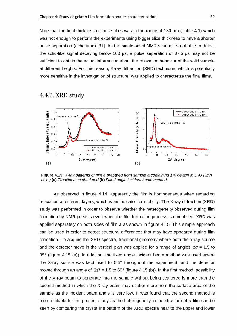
Chapter 4: Study of gelatin film formation and its characterization 52
Note that the final thickness of these films was in the range of 130 µm (Table 4.1) which
was not enough to perform the experiments using bigger slice thickness to have a shorter
pulse separation (echo time) [31]. As the single-sided NMR scanner is not able to detect
the solid-like signal decaying below 100 µs, a pulse separation of 87.5 µs may not be
sufficient to obtain the actual information about the relaxation behavior of the solid sample
at different heights. For this reason, X-ray diffraction (XRD) technique, which is potentially
more sensitive in the investigation of structure, was applied to characterize the final films.
4.4.2. XRD study
As observed in figure 4.14, apparently the film is homogeneous when regarding
relaxation at different layers, which is an indicator for mobility. The X-ray diffraction (XRD)
study was performed in order to observe whether the heterogeneity observed during film
formation by NMR persists even when the film formation process is completed. XRD was
applied separately on both sides of film a as shown in figure 4.15. This simple approach
can be used in order to detect structural differences that may have appeared during film
formation. To acquire the XRD spectra, traditional geometry where both the x-ray source
and the detector move in the vertical plan was applied for a range of angles 2 = 1.5 to
35° (figure 4.15 (a)). In addition, the fixed angle incident beam method was used where
the X-ray source was kept fixed to 0.5° throughout the experiment, and the detector
moved through an angle of 2 = 1.5 to 60° (figure 4.15 (b)). In the first method, possibility
of the X-ray beam to penetrate into the sample without being scattered is more than the
second method in which the X-ray beam may scatter more from the surface area of the
sample as the incident beam angle is very low. It was found that the second method is
more suitable for the present study as the heterogeneity in the structure of a film can be
seen by comparing the crystalline pattern of the XRD spectra near to the upper and lower
Figure 4.15: X-ray patterns of film a prepared from sample a containing 1% gelatin in D2O (w/v) using (a) Traditional method and (b) Fixed angle incident beam method.
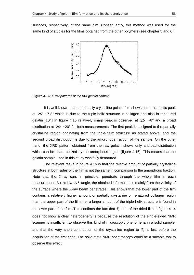
Chapter 4: Study of gelatin film formation and its characterization 53
surfaces, respectively, of the same film. Consequently, this method was used for the
same kind of studies for the films obtained from the other polymers (see chapter 5 and 6).
It is well known that the partially crystalline gelatin film shows a characteristic peak
at 2 ~7-8° which is due to the triple-helix structure in collagen and also in renatured
gelatin [104] In figure 4.15 relatively sharp peak is observed at 2 ~8° and a broad
distribution at 2 ~20° for both measurements. The first peak is assigned to the partially
crystalline region originating from the triple-helix structure as stated above, and the
second broad distribution is due to the amorphous fraction of the sample. On the other
hand, the XRD pattern obtained from the raw gelatin shows only a broad distribution
which can be characterized by the amorphous region (figure 4.16). This means that the
gelatin sample used in this study was fully denatured.
The relevant result in figure 4.15 is that the relative amount of partially crystalline
structure at both sides of the film is not the same in comparison to the amorphous fraction.
Note that the X-ray can, in principle, penetrate through the whole film in each
measurement. But at low 2 angle, the obtained information is mainly from the vicinity of
the surface where the X-ray beam penetrates. This shows that the lower part of the film
contains a relatively higher amount of partially crystalline or renatured collagen region
than the upper part of the film, i.e. a larger amount of the triple-helix structure is found in
the lower part of the film. This confirms the fact that 2
T data of the dried film in figure 4.14
does not show a clear heterogeneity is because the resolution of the single-sided NMR
scanner is insufficient to observe this kind of microscopic phenomena in a solid sample,
and that the very short contribution of the crystalline region to 2
T is lost before the
acquisition of the first echo. The solid-state NMR spectroscopy could be a suitable tool to
observe this effect.
Figure 4.16: X-ray patterns of the raw gelatin sample.
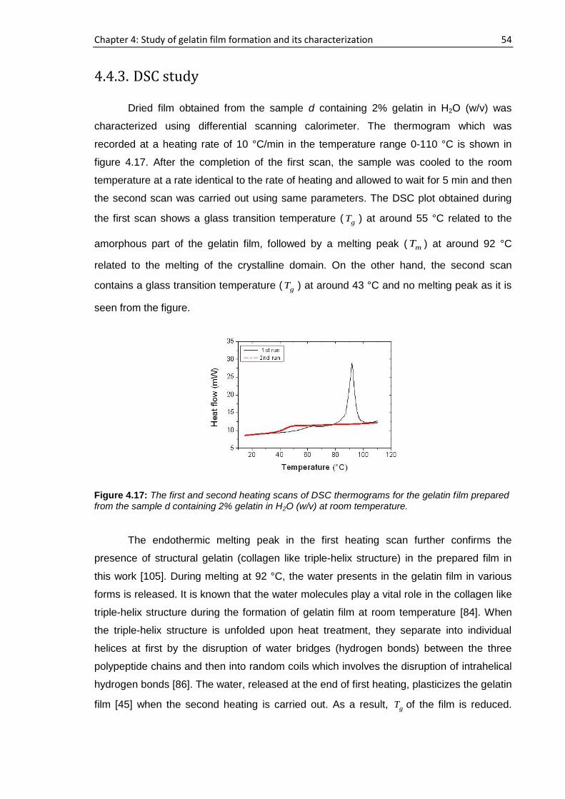
Chapter 4: Study of gelatin film formation and its characterization 54
4.4.3. DSC study
Dried film obtained from the sample d containing 2% gelatin in H2O (w/v) was
characterized using differential scanning calorimeter. The thermogram which was
recorded at a heating rate of 10 °C/min in the temperature range 0-110 °C is shown in
figure 4.17. After the completion of the first scan, the sample was cooled to the room
temperature at a rate identical to the rate of heating and allowed to wait for 5 min and then
the second scan was carried out using same parameters. The DSC plot obtained during
the first scan shows a glass transition temperature ( gT ) at around 55 °C related to the
amorphous part of the gelatin film, followed by a melting peak ( mT ) at around 92 °C
related to the melting of the crystalline domain. On the other hand, the second scan
contains a glass transition temperature ( gT ) at around 43 °C and no melting peak as it is
seen from the figure.
The endothermic melting peak in the first heating scan further confirms the
presence of structural gelatin (collagen like triple-helix structure) in the prepared film in
this work [105]. During melting at 92 °C, the water presents in the gelatin film in various
forms is released. It is known that the water molecules play a vital role in the collagen like
triple-helix structure during the formation of gelatin film at room temperature [84]. When
the triple-helix structure is unfolded upon heat treatment, they separate into individual
helices at first by the disruption of water bridges (hydrogen bonds) between the three
polypeptide chains and then into random coils which involves the disruption of intrahelical
hydrogen bonds [86]. The water, released at the end of first heating, plasticizes the gelatin
film [45] when the second heating is carried out. As a result, gT of the film is reduced.
Figure 4.17: The first and second heating scans of DSC thermograms for the gelatin film prepared from the sample d containing 2% gelatin in H2O (w/v) at room temperature.
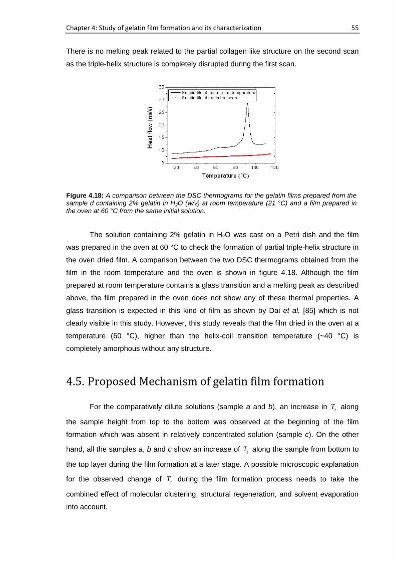
Chapter 4: Study of gelatin film formation and its characterization 55
There is no melting peak related to the partial collagen like structure on the second scan
as the triple-helix structure is completely disrupted during the first scan.
The solution containing 2% gelatin in H2O was cast on a Petri dish and the film
was prepared in the oven at 60 °C to check the formation of partial triple-helix structure in
the oven dried film. A comparison between the two DSC thermograms obtained from the
film in the room temperature and the oven is shown in figure 4.18. Although the film
prepared at room temperature contains a glass transition and a melting peak as described
above, the film prepared in the oven does not show any of these thermal properties. A
glass transition is expected in this kind of film as shown by Dai et al. [85] which is not
clearly visible in this study. However, this study reveals that the film dried in the oven at a
temperature (60 °C), higher than the helix-coil transition temperature (~40 °C) is
completely amorphous without any structure.
4.5. Proposed Mechanism of gelatin film formation
For the comparatively dilute solutions (sample a and b), an increase in 2
T along
the sample height from top to the bottom was observed at the beginning of the film
formation which was absent in relatively concentrated solution (sample c). On the other
hand, all the samples a, b and c show an increase of 2
T along the sample from bottom to
the top layer during the film formation at a later stage. A possible microscopic explanation
for the observed change of 2
T during the film formation process needs to take the
combined effect of molecular clustering, structural regeneration, and solvent evaporation
into account.
Figure 4.18: A comparison between the DSC thermograms for the gelatin films prepared from the sample d containing 2% gelatin in H2O (w/v) at room temperature (21 °C) and a film prepared in the oven at 60 °C from the same initial solution.
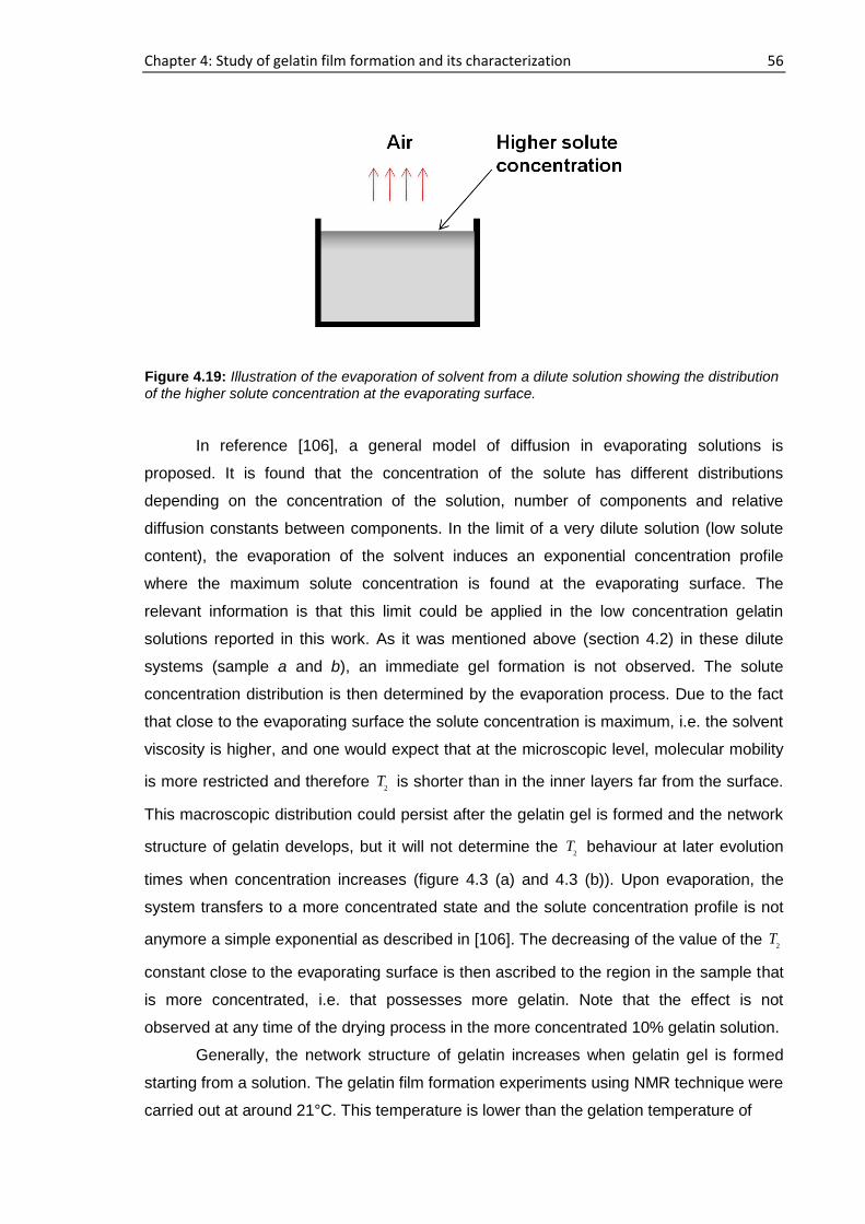
Chapter 4: Study of gelatin film formation and its characterization 56
In reference [106], a general model of diffusion in evaporating solutions is
proposed. It is found that the concentration of the solute has different distributions
depending on the concentration of the solution, number of components and relative
diffusion constants between components. In the limit of a very dilute solution (low solute
content), the evaporation of the solvent induces an exponential concentration profile
where the maximum solute concentration is found at the evaporating surface. The
relevant information is that this limit could be applied in the low concentration gelatin
solutions reported in this work. As it was mentioned above (section 4.2) in these dilute
systems (sample a and b), an immediate gel formation is not observed. The solute
concentration distribution is then determined by the evaporation process. Due to the fact
that close to the evaporating surface the solute concentration is maximum, i.e. the solvent
viscosity is higher, and one would expect that at the microscopic level, molecular mobility
is more restricted and therefore 2
T is shorter than in the inner layers far from the surface.
This macroscopic distribution could persist after the gelatin gel is formed and the network
structure of gelatin develops, but it will not determine the 2
T behaviour at later evolution
times when concentration increases (figure 4.3 (a) and 4.3 (b)). Upon evaporation, the
system transfers to a more concentrated state and the solute concentration profile is not
anymore a simple exponential as described in [106]. The decreasing of the value of the 2
T
constant close to the evaporating surface is then ascribed to the region in the sample that
is more concentrated, i.e. that possesses more gelatin. Note that the effect is not
observed at any time of the drying process in the more concentrated 10% gelatin solution.
Generally, the network structure of gelatin increases when gelatin gel is formed
starting from a solution. The gelatin film formation experiments using NMR technique were
carried out at around 21°C. This temperature is lower than the gelation temperature of
Figure 4.19: Illustration of the evaporation of solvent from a dilute solution showing the distribution of the higher solute concentration at the evaporating surface.
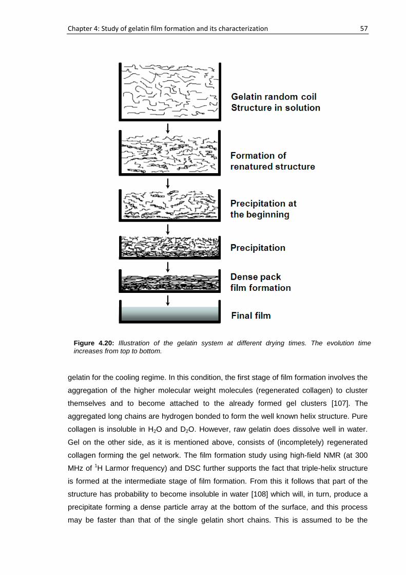
Chapter 4: Study of gelatin film formation and its characterization 57
gelatin for the cooling regime. In this condition, the first stage of film formation involves the
aggregation of the higher molecular weight molecules (regenerated collagen) to cluster
themselves and to become attached to the already formed gel clusters [107]. The
aggregated long chains are hydrogen bonded to form the well known helix structure. Pure
collagen is insoluble in H2O and D2O. However, raw gelatin does dissolve well in water.
Gel on the other side, as it is mentioned above, consists of (incompletely) regenerated
collagen forming the gel network. The film formation study using high-field NMR (at 300
MHz of 1H Larmor frequency) and DSC further supports the fact that triple-helix structure
is formed at the intermediate stage of film formation. From this it follows that part of the
structure has probability to become insoluble in water [108] which will, in turn, produce a
precipitate forming a dense particle array at the bottom of the surface, and this process
may be faster than that of the single gelatin short chains. This is assumed to be the
Figure 4.20: Illustration of the gelatin system at different drying times. The evolution time increases from top to bottom.
Chapter 4: Study of gelatin film formation and its characterization 58
second stage of the film formation. In this work, the reduction in 2
T and 1
T – both
indicating a decrease of mobility – was observed at different depths of the sample from
the beginning of this stage. This process has continued and the difference in both
relaxation times, but more dramatically in 2
T , increased from layer to layer. At the same
time, evaporation of the solvent results in an increasing total concentration in the sample.
In the final stage, residual solvent has evaporated giving a densely packed gel film with
only a small amount of residual water incorporated. The XRD data shows that the dense
triple-helix structure that is preferably generated at the bottom of the sample during the
evaporation makes a significant difference in the structure of the final film.
4.6. Concentration and humidity effects on gelatin films
In the study of gelatin film formation using single-sided NMR, it was observed that
the molecular dynamics of the gelatin polymer varies with the initial concentration of
gelatin in water at an early stage of film formation. For the relatively diluted solutions (1%
and 2% initial concentration of gelatin in D2O (w/v)), the distribution of the solute was
heterogeneous in the vicinity of the air-sample interface compared to the relatively
concentrated sample (10% initial concentration of gelatin in D2O (w/v)). Note that this
effect was observed when the concentration of the diluted solution was more than 10%
due to solvent evaporation (see section 4.3.1). This suggests that the initial concentration
of the gelatin solution plays a role in the molecular dynamics of the system during drying
as well as in the final film although one would expect that two solutions with initial
concentration 1
C and 2C , with 1 2
C C will have the same properties when 2C will reach
the same value as 1
C during drying. Motivated by this fact, gelatin films were prepared
from a wide initial concentration range (1% to 30%), and characterized using NMR, DSC
and TGA methods to obtain information about the effect of initial concentration of gelatin
on the final film. Another purpose of this study was to acquire information about the effect
of humidity on these gelatin films. Humidity is an important parameter to be considered for
the application of the gelatin film as it varies with the change of climate, for example,
relative humidity at tropical climate (averaging around 70%) is different than that of the
continental climate (averaging around 40%). Water content in gelatin film varies with the
change in humidity and it affects the mechanical properties of the film [84]. In this study,
gelatin films were equilibrated at four different relative humidities (RH) (20%, 43%, 75%
and 90%) before characterization (see below). Gelatin film was prepared from 9 different
initial concentrations (1%, 3%, 5%, 7%, 10%, 15%, 20%, 25% and 30% gelatin in H2O
(w/v)) using the procedure described in section 3.2.1.
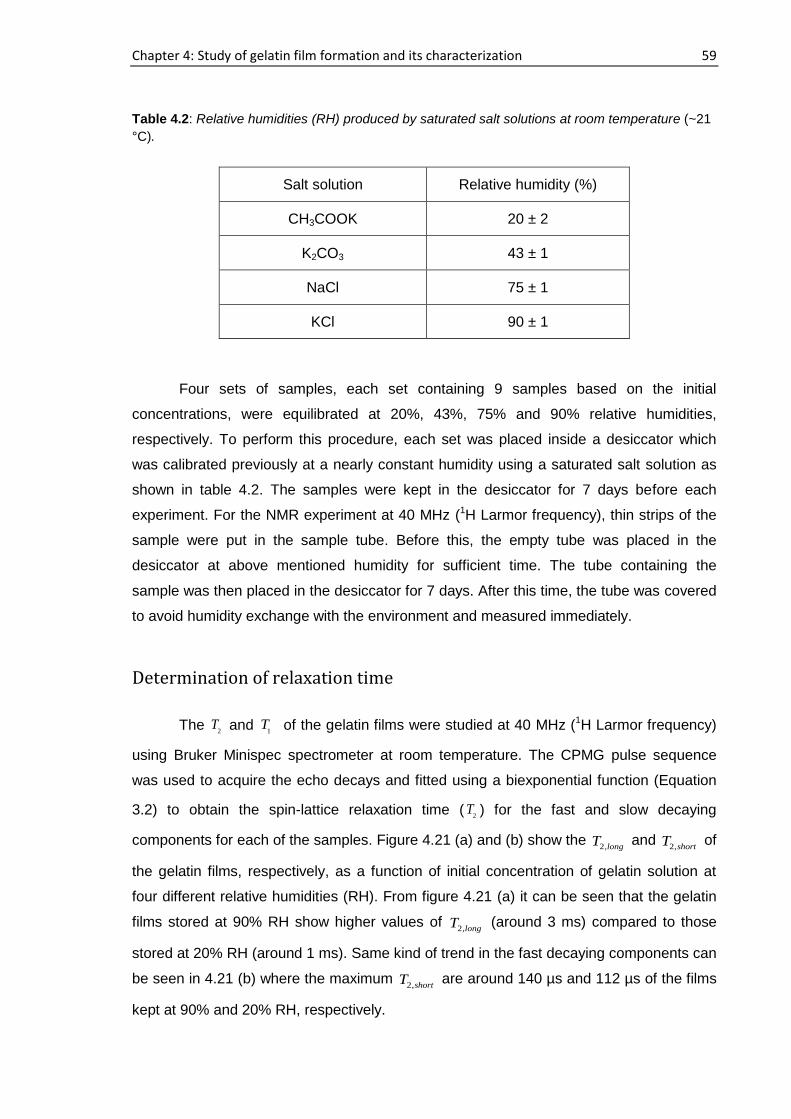
Chapter 4: Study of gelatin film formation and its characterization 59
Table 4.2: Relative humidities (RH) produced by saturated salt solutions at room temperature (~21
°C).
Salt solution Relative humidity (%)
CH3COOK 20 ± 2
K2CO3 43 ± 1
NaCl 75 ± 1
KCl 90 ± 1
Four sets of samples, each set containing 9 samples based on the initial
concentrations, were equilibrated at 20%, 43%, 75% and 90% relative humidities,
respectively. To perform this procedure, each set was placed inside a desiccator which
was calibrated previously at a nearly constant humidity using a saturated salt solution as
shown in table 4.2. The samples were kept in the desiccator for 7 days before each
experiment. For the NMR experiment at 40 MHz (1H Larmor frequency), thin strips of the
sample were put in the sample tube. Before this, the empty tube was placed in the
desiccator at above mentioned humidity for sufficient time. The tube containing the
sample was then placed in the desiccator for 7 days. After this time, the tube was covered
to avoid humidity exchange with the environment and measured immediately.
Determination of relaxation time
The 2
T and 1
T of the gelatin films were studied at 40 MHz (1H Larmor frequency)
using Bruker Minispec spectrometer at room temperature. The CPMG pulse sequence
was used to acquire the echo decays and fitted using a biexponential function (Equation
3.2) to obtain the spin-lattice relaxation time (2
T ) for the fast and slow decaying
components for each of the samples. Figure 4.21 (a) and (b) show the 2,longT and
2,shortT of
the gelatin films, respectively, as a function of initial concentration of gelatin solution at
four different relative humidities (RH). From figure 4.21 (a) it can be seen that the gelatin
films stored at 90% RH show higher values of 2,longT (around 3 ms) compared to those
stored at 20% RH (around 1 ms). Same kind of trend in the fast decaying components can
be seen in 4.21 (b) where the maximum 2,shortT are around 140 µs and 112 µs of the films
kept at 90% and 20% RH, respectively.
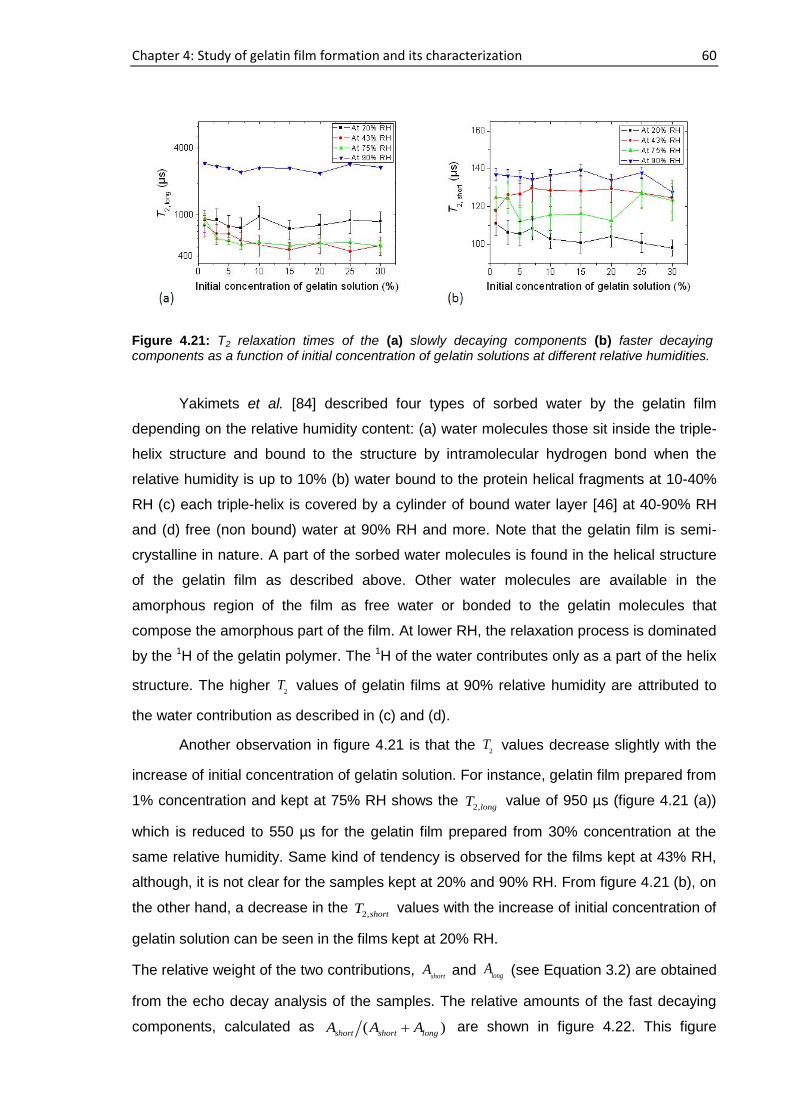
Chapter 4: Study of gelatin film formation and its characterization 60
Yakimets et al. [84] described four types of sorbed water by the gelatin film
depending on the relative humidity content: (a) water molecules those sit inside the triple-
helix structure and bound to the structure by intramolecular hydrogen bond when the
relative humidity is up to 10% (b) water bound to the protein helical fragments at 10-40%
RH (c) each triple-helix is covered by a cylinder of bound water layer [46] at 40-90% RH
and (d) free (non bound) water at 90% RH and more. Note that the gelatin film is semi-
crystalline in nature. A part of the sorbed water molecules is found in the helical structure
of the gelatin film as described above. Other water molecules are available in the
amorphous region of the film as free water or bonded to the gelatin molecules that
compose the amorphous part of the film. At lower RH, the relaxation process is dominated
by the 1H of the gelatin polymer. The 1H of the water contributes only as a part of the helix
structure. The higher 2
T values of gelatin films at 90% relative humidity are attributed to
the water contribution as described in (c) and (d).
Another observation in figure 4.21 is that the 2
T values decrease slightly with the
increase of initial concentration of gelatin solution. For instance, gelatin film prepared from
1% concentration and kept at 75% RH shows the 2,longT value of 950 µs (figure 4.21 (a))
which is reduced to 550 µs for the gelatin film prepared from 30% concentration at the
same relative humidity. Same kind of tendency is observed for the films kept at 43% RH,
although, it is not clear for the samples kept at 20% and 90% RH. From figure 4.21 (b), on
the other hand, a decrease in the 2,shortT values with the increase of initial concentration of
gelatin solution can be seen in the films kept at 20% RH.
The relative weight of the two contributions, short
A and longA (see Equation 3.2) are obtained
from the echo decay analysis of the samples. The relative amounts of the fast decaying
components, calculated as ( )short short longA A A are shown in figure 4.22. This figure
Figure 4.21: T2 relaxation times of the (a) slowly decaying components (b) faster decaying components as a function of initial concentration of gelatin solutions at different relative humidities.

Chapter 4: Study of gelatin film formation and its characterization 61
demonstrates that there is an initial gelatin concentration dependency on the fast
decaying components of the films kept at higher relative humidities. At 75% and 90% RH,
relative amount of the fast decaying components are lower in the gelatin films prepared
from the higher gelatin concentrations compared with those prepared from lower
concentrations.
An inversion recovery pulse sequence [180 90 ] was used with 30 values
(logarithmically spaced) to measure the spin-lattice relaxation time (1
T ). Figure 4.23
shows the 1
T values as a function of initial concentration of gelatin solution at four
different relative humidities. In this study, the 1
T values of only one component were
detected from all the samples at different humidities. This means that the 1
T relaxation
times obtained here refer to the interaction between the excited 1H of the gelatin polymer
as well as different types of water molecules in the gelatin film and the lattice molecules
Figure 4.22: Relative amount of fast decaying components as a function of initial concentration of gelatin solution at different relative humidities.
Figure 4.23: T1 relaxation times as a function of initial concentration of gelatin solution at different relative humidities.
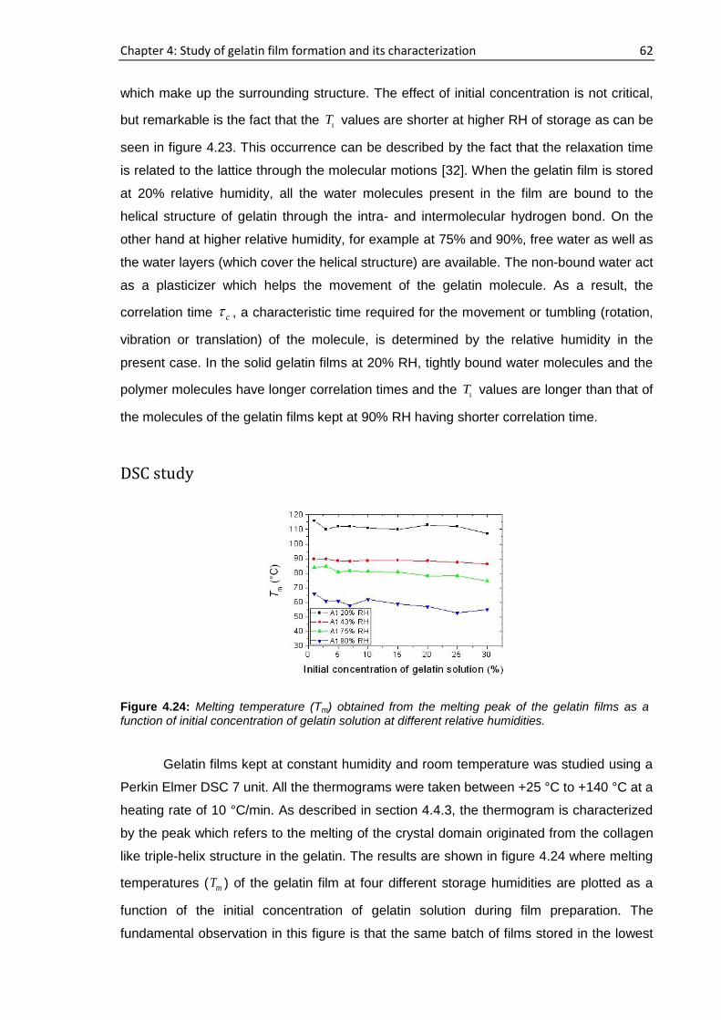
Chapter 4: Study of gelatin film formation and its characterization 62
which make up the surrounding structure. The effect of initial concentration is not critical,
but remarkable is the fact that the 1
T values are shorter at higher RH of storage as can be
seen in figure 4.23. This occurrence can be described by the fact that the relaxation time
is related to the lattice through the molecular motions [32]. When the gelatin film is stored
at 20% relative humidity, all the water molecules present in the film are bound to the
helical structure of gelatin through the intra- and intermolecular hydrogen bond. On the
other hand at higher relative humidity, for example at 75% and 90%, free water as well as
the water layers (which cover the helical structure) are available. The non-bound water act
as a plasticizer which helps the movement of the gelatin molecule. As a result, the
correlation time c , a characteristic time required for the movement or tumbling (rotation,
vibration or translation) of the molecule, is determined by the relative humidity in the
present case. In the solid gelatin films at 20% RH, tightly bound water molecules and the
polymer molecules have longer correlation times and the 1
T values are longer than that of
the molecules of the gelatin films kept at 90% RH having shorter correlation time.
DSC study
Gelatin films kept at constant humidity and room temperature was studied using a
Perkin Elmer DSC 7 unit. All the thermograms were taken between +25 °C to +140 °C at a
heating rate of 10 °C/min. As described in section 4.4.3, the thermogram is characterized
by the peak which refers to the melting of the crystal domain originated from the collagen
like triple-helix structure in the gelatin. The results are shown in figure 4.24 where melting
temperatures ( mT ) of the gelatin film at four different storage humidities are plotted as a
function of the initial concentration of gelatin solution during film preparation. The
fundamental observation in this figure is that the same batch of films stored in the lowest
Figure 4.24: Melting temperature (Tm) obtained from the melting peak of the gelatin films as a function of initial concentration of gelatin solution at different relative humidities.
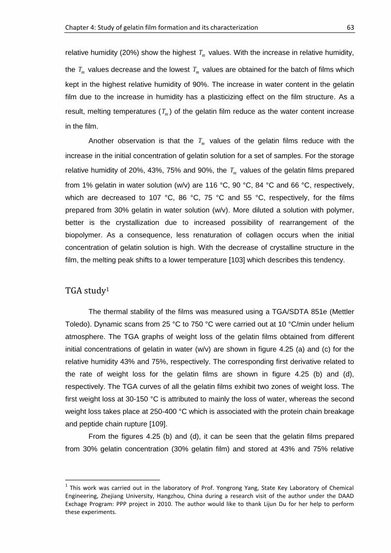
Chapter 4: Study of gelatin film formation and its characterization 63
relative humidity (20%) show the highest mT values. With the increase in relative humidity,
the mT values decrease and the lowest mT values are obtained for the batch of films which
kept in the highest relative humidity of 90%. The increase in water content in the gelatin
film due to the increase in humidity has a plasticizing effect on the film structure. As a
result, melting temperatures ( mT ) of the gelatin film reduce as the water content increase
in the film.
Another observation is that the mT values of the gelatin films reduce with the
increase in the initial concentration of gelatin solution for a set of samples. For the storage
relative humidity of 20%, 43%, 75% and 90%, the mT values of the gelatin films prepared
from 1% gelatin in water solution (w/v) are 116 °C, 90 °C, 84 °C and 66 °C, respectively,
which are decreased to 107 °C, 86 °C, 75 °C and 55 °C, respectively, for the films
prepared from 30% gelatin in water solution (w/v). More diluted a solution with polymer,
better is the crystallization due to increased possibility of rearrangement of the
biopolymer. As a consequence, less renaturation of collagen occurs when the initial
concentration of gelatin solution is high. With the decrease of crystalline structure in the
film, the melting peak shifts to a lower temperature [103] which describes this tendency.
TGA study1
The thermal stability of the films was measured using a TGA/SDTA 851e (Mettler
Toledo). Dynamic scans from 25 °C to 750 °C were carried out at 10 °C/min under helium
atmosphere. The TGA graphs of weight loss of the gelatin films obtained from different
initial concentrations of gelatin in water (w/v) are shown in figure 4.25 (a) and (c) for the
relative humidity 43% and 75%, respectively. The corresponding first derivative related to
the rate of weight loss for the gelatin films are shown in figure 4.25 (b) and (d),
respectively. The TGA curves of all the gelatin films exhibit two zones of weight loss. The
first weight loss at 30-150 °C is attributed to mainly the loss of water, whereas the second
weight loss takes place at 250-400 °C which is associated with the protein chain breakage
and peptide chain rupture [109].
From the figures 4.25 (b) and (d), it can be seen that the gelatin films prepared
from 30% gelatin concentration (30% gelatin film) and stored at 43% and 75% relative
1 This work was carried out in the laboratory of Prof. Yongrong Yang, State Key Laboratory of Chemical
Engineering, Zhejiang University, Hangzhou, China during a research visit of the author under the DAAD Exchage Program: PPP project in 2010. The author would like to thank Lijun Du for her help to perform these experiments.
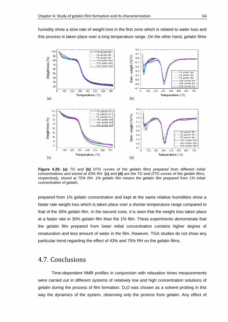
Chapter 4: Study of gelatin film formation and its characterization 64
humidity show a slow rate of weight loss in the first zone which is related to water loss and
this process is taken place over a long temperature range. On the other hand, gelatin films
prepared from 1% gelatin concentration and kept at the same relative humidities show a
faster rate weight loss which is taken place over a shorter temperature range compared to
that of the 30% gelatin film. In the second zone, it is seen that the weight loss taken place
at a faster rate in 30% gelatin film than the 1% film. These experiments demonstrate that
the gelatin film prepared from lower initial concentration contains higher degree of
renaturation and less amount of water in the film. However, TGA studies do not show any
particular trend regarding the effect of 43% and 75% RH on the gelatin films.
4.7. Conclusions
Time-dependent NMR profiles in conjunction with relaxation times measurements
were carried out in different systems of relatively low and high concentration solutions of
gelatin during the process of film formation. D2O was chosen as a solvent probing in this
way the dynamics of the system, observing only the protons from gelatin. Any effect of
Figure 4.25: (a) TG and (b) DTG curves of the gelatin films prepared from different initial concentrations and stored at 43% RH. (c) and (d) are the TG and DTG curves of the gelatin films, respectively, stored at 75% RH. 1% gelatin film means the gelatin film prepared from 1% initial concentration of gelatin.
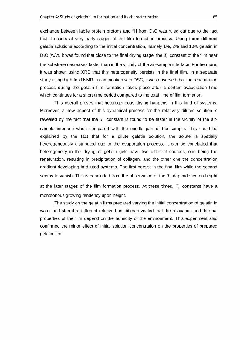
Chapter 4: Study of gelatin film formation and its characterization 65
exchange between labile protein protons and 2H from D2O was ruled out due to the fact
that it occurs at very early stages of the film formation process. Using three different
gelatin solutions according to the initial concentration, namely 1%, 2% and 10% gelatin in
D2O (w/v), it was found that close to the final drying stage, the 2
T constant of the film near
the substrate decreases faster than in the vicinity of the air-sample interface. Furthermore,
it was shown using XRD that this heterogeneity persists in the final film. In a separate
study using high-field NMR in combination with DSC, it was observed that the renaturation
process during the gelatin film formation takes place after a certain evaporation time
which continues for a short time period compared to the total time of film formation.
This overall proves that heterogeneous drying happens in this kind of systems.
Moreover, a new aspect of this dynamical process for the relatively diluted solution is
revealed by the fact that the 2
T constant is found to be faster in the vicinity of the air-
sample interface when compared with the middle part of the sample. This could be
explained by the fact that for a dilute gelatin solution, the solute is spatially
heterogeneously distributed due to the evaporation process. It can be concluded that
heterogeneity in the drying of gelatin gels have two different sources, one being the
renaturation, resulting in precipitation of collagen, and the other one the concentration
gradient developing in diluted systems. The first persist in the final film while the second
seems to vanish. This is concluded from the observation of the 2
T dependence on height
at the later stages of the film formation process. At these times, 2
T constants have a
monotonous growing tendency upon height.
The study on the gelatin films prepared varying the initial concentration of gelatin in
water and stored at different relative humidities revealed that the relaxation and thermal
properties of the film depend on the humidity of the environment. This experiment also
confirmed the minor effect of initial solution concentration on the properties of prepared
gelatin film.
66
Chapter 5
Starch film formation study
If you have an apple and I have an apple and we exchange these apples then you and I will still
each have one apple. But if you have an idea and I have an idea and we exchange these ideas,
then each of us will have two ideas.
George Bernard Shaw
5.1. Introduction
Starch granule is composed of three different regions which are amorphous region,
crystalline lamellae and amorphous growth ring. At room temperature, a starch granule is
not soluble in water because of the stable semi-crystalline structure. However, it
undergoes limited swelling (reversible), presumably due to hydration and swelling of the
amorphous regions. It is known that amylopectin (figure 3.2 (b)), due to its highly
branched open structure, allows access to hydrogen-bonding solvent molecule.
Consequently it is more disrupted in water or another solvent able to form hydrogen
bonding than amylose, which has a tightly packed structure. The interaction of starch
granules with hot water is different as in water at room temperature. For example, when
the starch granules are heated in excess water beyond a critical temperature depending
on the type of starch, an irreversible change is taken place known as gelatinization [16].
This involves swelling of the granules, crystallite melting, viscosity development and
solubilization. During swelling, the amorphous phase of granular starch is fully plasticized
by the solvent and amylose (figure 3.2 (a)) starts to leach. This process is influenced by
the increase in temperature. Depending on the initial concentration of starch in water, a
precipitation or a white elastic gel (prepared from a concentrated system) can be obtained
when the system is left at rest and cool down to room temperature [68]. Apart from the
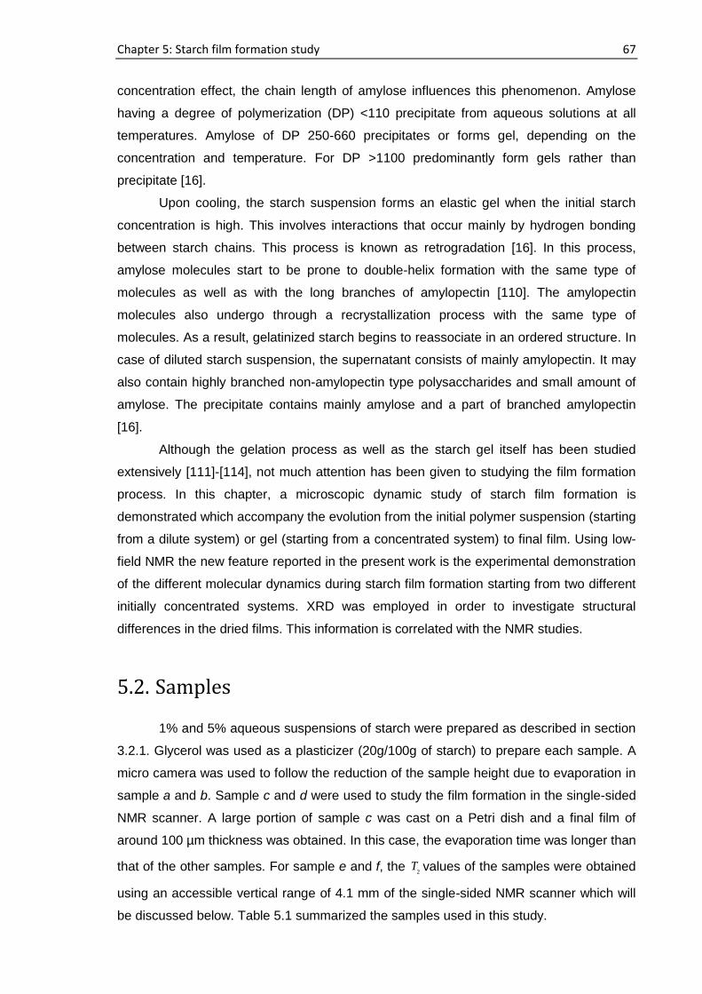
Chapter 5: Starch film formation study 67
concentration effect, the chain length of amylose influences this phenomenon. Amylose
having a degree of polymerization (DP) <110 precipitate from aqueous solutions at all
temperatures. Amylose of DP 250-660 precipitates or forms gel, depending on the
concentration and temperature. For DP >1100 predominantly form gels rather than
precipitate [16].
Upon cooling, the starch suspension forms an elastic gel when the initial starch
concentration is high. This involves interactions that occur mainly by hydrogen bonding
between starch chains. This process is known as retrogradation [16]. In this process,
amylose molecules start to be prone to double-helix formation with the same type of
molecules as well as with the long branches of amylopectin [110]. The amylopectin
molecules also undergo through a recrystallization process with the same type of
molecules. As a result, gelatinized starch begins to reassociate in an ordered structure. In
case of diluted starch suspension, the supernatant consists of mainly amylopectin. It may
also contain highly branched non-amylopectin type polysaccharides and small amount of
amylose. The precipitate contains mainly amylose and a part of branched amylopectin
[16].
Although the gelation process as well as the starch gel itself has been studied
extensively [111]-[114], not much attention has been given to studying the film formation
process. In this chapter, a microscopic dynamic study of starch film formation is
demonstrated which accompany the evolution from the initial polymer suspension (starting
from a dilute system) or gel (starting from a concentrated system) to final film. Using low-
field NMR the new feature reported in the present work is the experimental demonstration
of the different molecular dynamics during starch film formation starting from two different
initially concentrated systems. XRD was employed in order to investigate structural
differences in the dried films. This information is correlated with the NMR studies.
5.2. Samples
1% and 5% aqueous suspensions of starch were prepared as described in section
3.2.1. Glycerol was used as a plasticizer (20g/100g of starch) to prepare each sample. A
micro camera was used to follow the reduction of the sample height due to evaporation in
sample a and b. Sample c and d were used to study the film formation in the single-sided
NMR scanner. A large portion of sample c was cast on a Petri dish and a final film of
around 100 µm thickness was obtained. In this case, the evaporation time was longer than
that of the other samples. For sample e and f, the 2
T values of the samples were obtained
using an accessible vertical range of 4.1 mm of the single-sided NMR scanner which will
be discussed below. Table 5.1 summarized the samples used in this study.
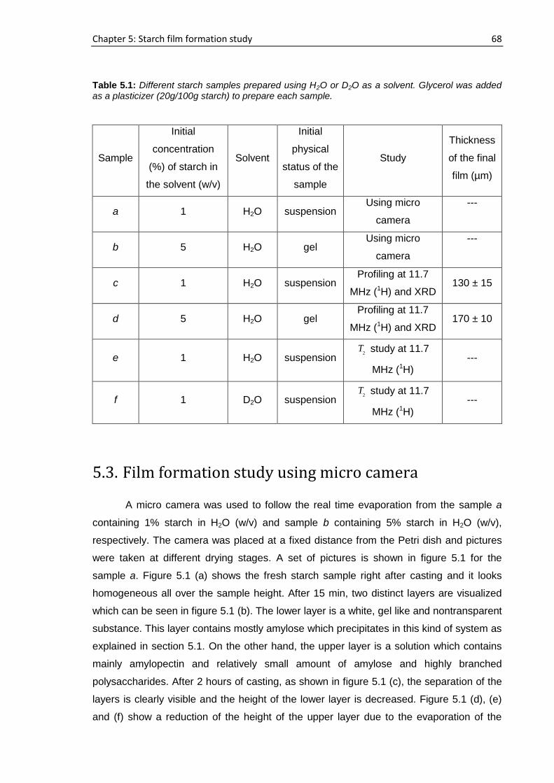
Chapter 5: Starch film formation study 68
Table 5.1: Different starch samples prepared using H2O or D2O as a solvent. Glycerol was added as a plasticizer (20g/100g starch) to prepare each sample.
Sample
Initial
concentration
(%) of starch in
the solvent (w/v)
Solvent
Initial
physical
status of the
sample
Study
Thickness
of the final
film (µm)
a 1 H2O suspension Using micro
camera
---
b 5 H2O gel Using micro
camera
---
c 1 H2O suspension Profiling at 11.7
MHz (1H) and XRD 130 ± 15
d 5 H2O gel Profiling at 11.7
MHz (1H) and XRD 170 ± 10
e 1 H2O suspension 2
T study at 11.7
MHz (1H) ---
f 1 D2O suspension 2
T study at 11.7
MHz (1H)
---
5.3. Film formation study using micro camera
A micro camera was used to follow the real time evaporation from the sample a
containing 1% starch in H2O (w/v) and sample b containing 5% starch in H2O (w/v),
respectively. The camera was placed at a fixed distance from the Petri dish and pictures
were taken at different drying stages. A set of pictures is shown in figure 5.1 for the
sample a. Figure 5.1 (a) shows the fresh starch sample right after casting and it looks
homogeneous all over the sample height. After 15 min, two distinct layers are visualized
which can be seen in figure 5.1 (b). The lower layer is a white, gel like and nontransparent
substance. This layer contains mostly amylose which precipitates in this kind of system as
explained in section 5.1. On the other hand, the upper layer is a solution which contains
mainly amylopectin and relatively small amount of amylose and highly branched
polysaccharides. After 2 hours of casting, as shown in figure 5.1 (c), the separation of the
layers is clearly visible and the height of the lower layer is decreased. Figure 5.1 (d), (e)
and (f) show a reduction of the height of the upper layer due to the evaporation of the
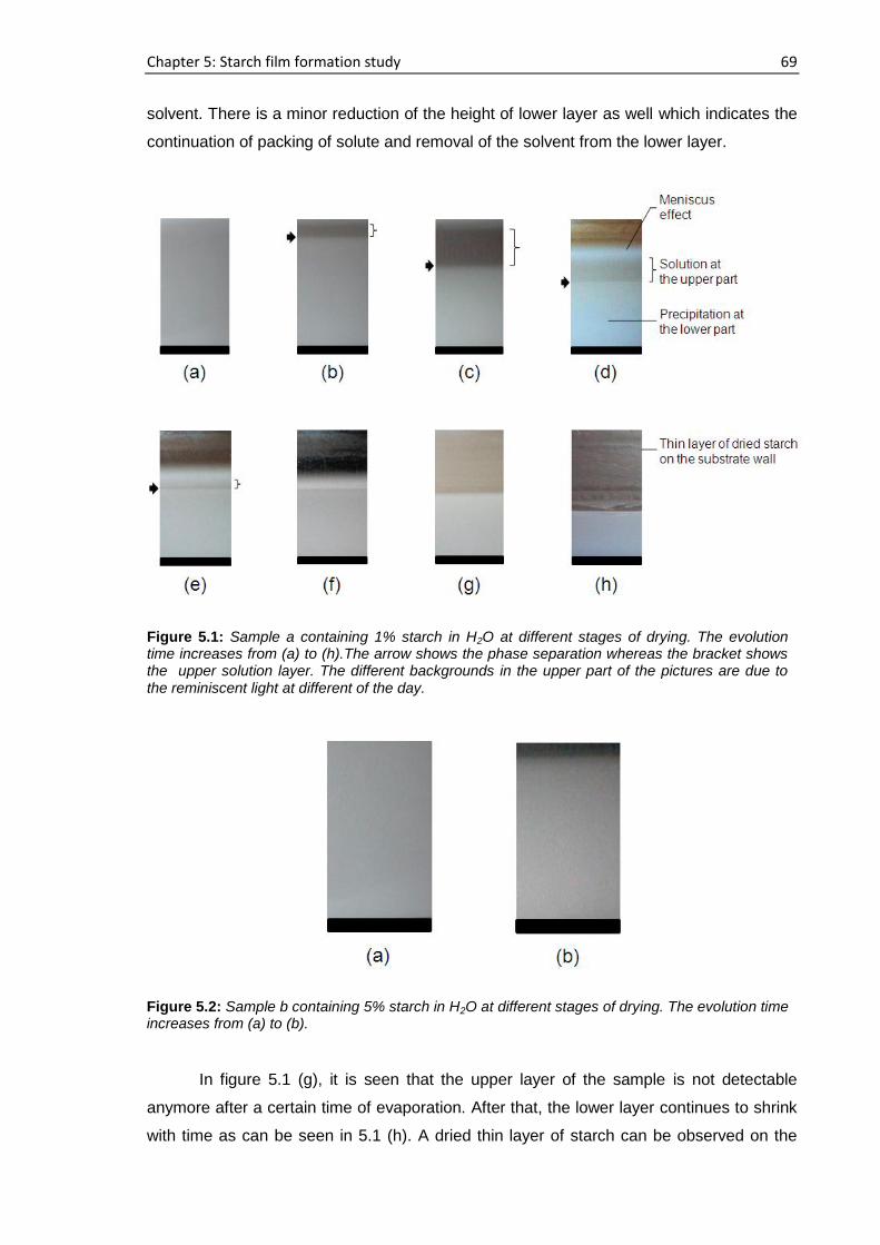
Chapter 5: Starch film formation study 69
solvent. There is a minor reduction of the height of lower layer as well which indicates the
continuation of packing of solute and removal of the solvent from the lower layer.
In figure 5.1 (g), it is seen that the upper layer of the sample is not detectable
anymore after a certain time of evaporation. After that, the lower layer continues to shrink
with time as can be seen in 5.1 (h). A dried thin layer of starch can be observed on the
Figure 5.1: Sample a containing 1% starch in H2O at different stages of drying. The evolution time increases from (a) to (h).The arrow shows the phase separation whereas the bracket shows the upper solution layer. The different backgrounds in the upper part of the pictures are due to the reminiscent light at different of the day.
Figure 5.2: Sample b containing 5% starch in H2O at different stages of drying. The evolution time increases from (a) to (b).
Chapter 5: Starch film formation study 70
wall of the Petri dish. The camera was fixed in order to cover the complete sample from
the beginning of the evaporation process. A meniscus on the top of the sample is clearly
visible in figure 5.1 (d) which blur the air-sample interface of the sample as can be seen in
figure 5.1 (e) and (f) as well. The concentration of the non-volatile components will be
increased at the upper part of the sample with the solvent evaporation. After a certain
drying time when the solvent is mostly evaporated from the upper part (as shown in figure
5.1 (f), in the present case), these components will apparently increase the thickness of
the lower part of the sample. This effect is not seen which might be due to the lack of
contrast or the presence of meniscus as described above.
Figure 5.2 shows the sample b which is prepared using 5% starch in H2O (w/v) and
cast on a Petri dish. The viscosity of this sample was high after gelatinization and it
formed a gel as can be seen in 5.2. Due to retrogradation, amylose and amylopectin
present in the system form an ordered structure. As the solvent evaporates, the sample
thickness decreased with time and the film was formed.
5.4. Real time film formation study using single-sided
NMR scanner
Profiling of the samples
When the height of the starch sample was approximately 1 mm following partial
evaporation of H2O, it was placed on to the single-sided NMR scanning device. The
starting time of the profile experiments is considered as time, t=0 in the following
discussion. For sample c, this time corresponds to 78 h after the casting time whereas 38
h had elapsed for sample d. After 78 h of casting time, water was already evaporated from
the top layer of sample c (corresponding to the phase rich in amylopectin) and became
similar to sample a in figure 5.1 (h). On the other hand, sample d was in gel state after 38
h.
For both samples, 23 consecutive experiments, i.e. complete profiles, were carried
out as shown in figure 5.3 (a) and (b) for sample c containing 1% starch in H2O (w/v) and
sample d containing 5% starch in H2O (w/v), respectively. The direction of scanning was
from top (sample-air interface) to bottom (sample-substrate interface). The position of the
sensor was moved in steps of 100 µm until 277 min and 417 min for sample c and d,
respectively, after which it was reduced to 50 µm. The figure shows that the height of the
samples exceeds the scanning range of the machine. The resolution was fixed to 50 µm in
both cases. 12 and 15 points were required for sample c and d, respectively, to cover the

Chapter 5: Starch film formation study 71
space between the substrate – defined as zero in the following discussion – and the
sample-air interface. For sample c, with a pulse separation of 87.5 µs, 32 scans, 2048
echoes and 8 s repetition time, a total time of ~256 s was required for the acquisition of
data at one position, i.e. one individual slice. That means the time for scanning the full
profile was ~52 min. This period was followed by a waiting time of 23 min. In sample d, the
repetition time was reduced to 7 s and the number of scans was the same, so that each
profile took 56 min to be completed; this period was followed by a waiting time of 34 min
before the beginning of the following slice.
With the solvent evaporation in both samples, less time was required to
accumulate one profile as less repetition time was required at the later stage. The
repetition time was always adjusted to be ≥ 5 1
T for the full recovery of the magnetization
throughout the experiment. Although sample d contains higher amount of starch and
glycerol compared with sample c, both experiments show same maximum intensity (within
experimental error) in the initial profiles. A reduction in the signal intensity is observed
after about 737 min and 929 min for sample c and d, respectively, after being constant
Figure 5.3: NMR profiles of the starch-water system at different drying times: (a) Sample c containing 1% starch in H2O (w/v) and (b) Sample d containing 5% starch in H2O (w/v). Each sample contains glycerol (20g/100g of starch) as a plasticizer.
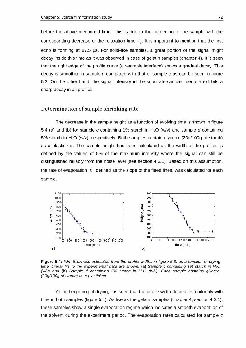
Chapter 5: Starch film formation study 72
before the above mentioned time. This is due to the hardening of the sample with the
corresponding decrease of the relaxation time 2
T . It is important to mention that the first
echo is forming at 87.5 µs. For solid-like samples, a great portion of the signal might
decay inside this time as it was observed in case of gelatin samples (chapter 4). It is seen
that the right edge of the profile curve (air-sample interface) shows a gradual decay. This
decay is smoother in sample d compared with that of sample c as can be seen in figure
5.3. On the other hand, the signal intensity in the substrate-sample interface exhibits a
sharp decay in all profiles.
Determination of sample shrinking rate
The decrease in the sample height as a function of evolving time is shown in figure
5.4 (a) and (b) for sample c containing 1% starch in H2O (w/v) and sample d containing
5% starch in H2O (w/v), respectively. Both samples contain glycerol (20g/100g of starch)
as a plasticizer. The sample height has been calculated as the width of the profiles is
defined by the values of 5% of the maximum intensity where the signal can still be
distinguished reliably from the noise level (see section 4.3.1). Based on this assumption,
the rate of evaporation E , defined as the slope of the fitted lines, was calculated for each
sample.
At the beginning of drying, it is seen that the profile width decreases uniformly with
time in both samples (figure 5.4). As like as the gelatin samples (chapter 4, section 4.3.1),
these samples show a single evaporation regime which indicates a smooth evaporation of
the solvent during the experiment period. The evaporation rates calculated for sample c
Figure 5.4: Film thickness estimated from the profile widths in figure 5.3, as a function of drying time. Linear fits to the experimental data are shown. (a) Sample c containing 1% starch in H2O (w/v) and (b) Sample d containing 5% starch in H2O (w/v). Each sample contains glycerol (20g/100g of starch) as a plasticizer.

Chapter 5: Starch film formation study 73
and d are 81.6 10
m/s and 8
2.1 10
m/s, respectively. After 1070 min and 1480 min, there
is no notable change in the profile widths of sample c and d (within the experimental error)
until the end of the experiment as can be seen in figure 5.4 (a) and (b), respectively.
The final profile width of these samples is in the range of 230 µm although the
actual thickness of the films is lower than this calculated value as can be seen in table 5.1.
After the profile experiments, all the films were stored in the same environmental
conditions as it was during the drying period to ensure complete drying of the film.
Determination of 2T at different heights
For both samples, the CPMG echo decay obtained from each profile point is
monoexponential at the earlier evaporation time. Accordingly, a mono-exponential
function (Equation 3.1) is fitted to the experimental data to obtain the spin-spin relaxation
time (2
T ) constant. At a later stage of drying, the decay curves obtained from the bottom
to a certain height of the sample could be fitted with two exponential decays (Equation
3.2).
Figure 5.5 (a) and (b) show the 2
T values obtained either from the single
component at an earlier stage or a combination of single and slow decaying components
(long component) at later stage during the total drying time with respect to different
positions in the sample c containing 1% starch in H2O (w/v) and sample d containing 5%
starch in H2O (w/v), respectively. Both samples contain glycerol (20g/100g of starch) as a
plasticizer. In general, both samples have nearly the same 2
T values at the beginning of
Figure 5.5: T2 constants at different heights of the sample. (a) Sample c containing 1% starch in H2O (w/v) and (b) Sample d containing 5% starch in H2O (w/v). Each sample contains glycerol (20g/100g of starch) as a plasticizer. Layer positions correspond to coordinates introduced in figure 5.3. At the later stage of drying, the echo decays were fitted with two exponential decay function from the bottom of the sample to a certain height which is showed by the arrow. In the case of bi-exponential decay, the effective T2 data showed in both figures correspond to the slow decaying components.
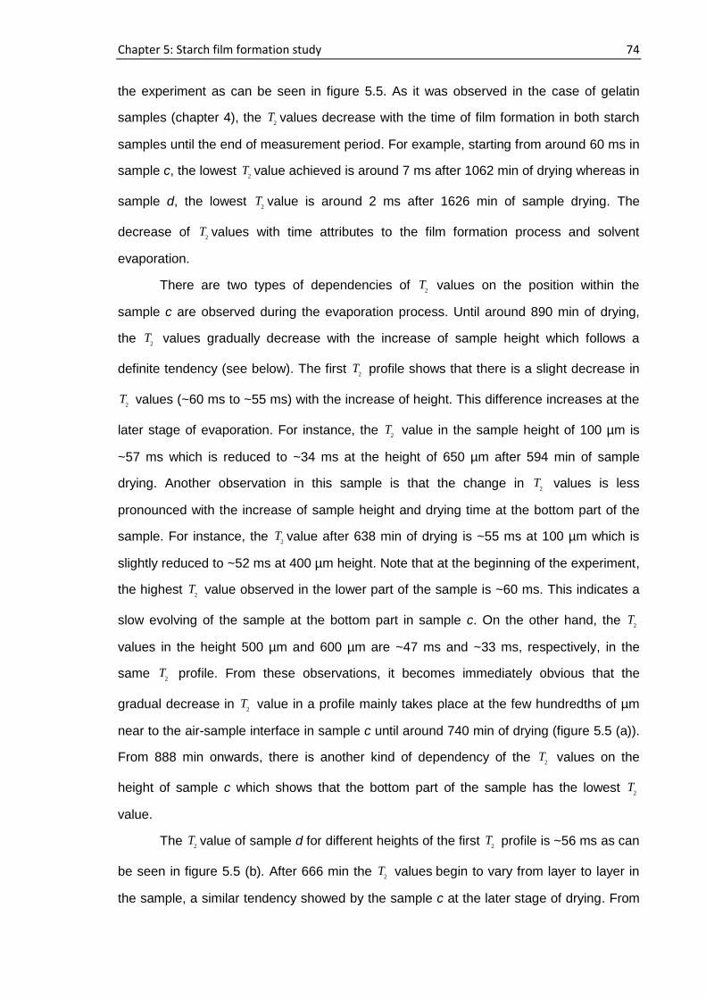
Chapter 5: Starch film formation study 74
the experiment as can be seen in figure 5.5. As it was observed in the case of gelatin
samples (chapter 4), the 2
T values decrease with the time of film formation in both starch
samples until the end of measurement period. For example, starting from around 60 ms in
sample c, the lowest 2
T value achieved is around 7 ms after 1062 min of drying whereas in
sample d, the lowest 2
T value is around 2 ms after 1626 min of sample drying. The
decrease of 2
T values with time attributes to the film formation process and solvent
evaporation.
There are two types of dependencies of 2
T values on the position within the
sample c are observed during the evaporation process. Until around 890 min of drying,
the 2
T values gradually decrease with the increase of sample height which follows a
definite tendency (see below). The first 2
T profile shows that there is a slight decrease in
2T values (~60 ms to ~55 ms) with the increase of height. This difference increases at the
later stage of evaporation. For instance, the 2
T value in the sample height of 100 µm is
~57 ms which is reduced to ~34 ms at the height of 650 µm after 594 min of sample
drying. Another observation in this sample is that the change in 2
T
values is less
pronounced with the increase of sample height and drying time at the bottom part of the
sample. For instance, the 2
T value after 638 min of drying is ~55 ms at 100 µm which is
slightly reduced to ~52 ms at 400 µm height. Note that at the beginning of the experiment,
the highest 2
T value observed in the lower part of the sample is ~60 ms. This indicates a
slow evolving of the sample at the bottom part in sample c. On the other hand, the 2
T
values in the height 500 µm and 600 µm are ~47 ms and ~33 ms, respectively, in the
same 2
T profile. From these observations, it becomes immediately obvious that the
gradual decrease in 2
T value in a profile mainly takes place at the few hundredths of µm
near to the air-sample interface in sample c until around 740 min of drying (figure 5.5 (a)).
From 888 min onwards, there is another kind of dependency of the 2
T values on the
height of sample c which shows that the bottom part of the sample has the lowest 2
T
value.
The 2
T value of sample d for different heights of the first 2
T profile is ~56 ms as can
be seen in figure 5.5 (b). After 666 min the 2
T values begin to vary from layer to layer in
the sample, a similar tendency showed by the sample c at the later stage of drying. From
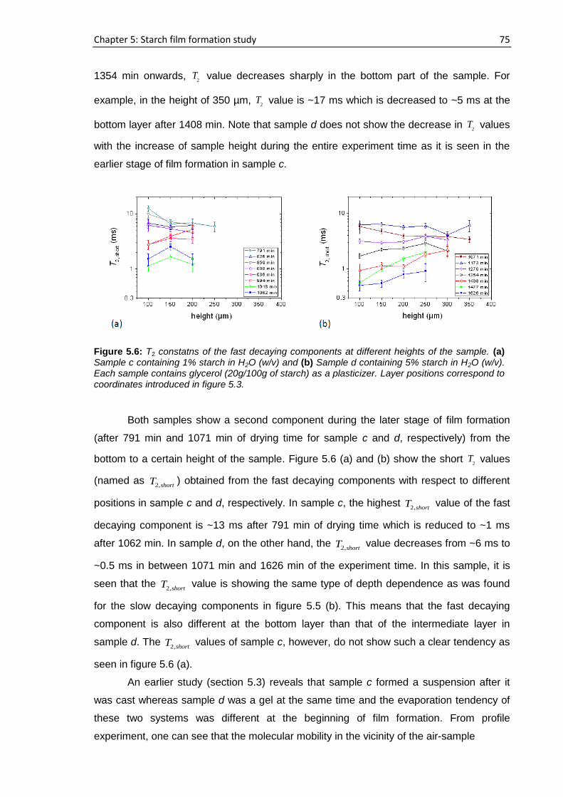
Chapter 5: Starch film formation study 75
1354 min onwards, 2
T value decreases sharply in the bottom part of the sample. For
example, in the height of 350 µm, 2
T value is ~17 ms which is decreased to ~5 ms at the
bottom layer after 1408 min. Note that sample d does not show the decrease in 2
T values
with the increase of sample height during the entire experiment time as it is seen in the
earlier stage of film formation in sample c.
Both samples show a second component during the later stage of film formation
(after 791 min and 1071 min of drying time for sample c and d, respectively) from the
bottom to a certain height of the sample. Figure 5.6 (a) and (b) show the short 2
T values
(named as 2,shortT ) obtained from the fast decaying components with respect to different
positions in sample c and d, respectively. In sample c, the highest 2,shortT value of the fast
decaying component is ~13 ms after 791 min of drying time which is reduced to ~1 ms
after 1062 min. In sample d, on the other hand, the 2,shortT value decreases from ~6 ms to
~0.5 ms in between 1071 min and 1626 min of the experiment time. In this sample, it is
seen that the 2,shortT value is showing the same type of depth dependence as was found
for the slow decaying components in figure 5.5 (b). This means that the fast decaying
component is also different at the bottom layer than that of the intermediate layer in
sample d. The 2,shortT values of sample c, however, do not show such a clear tendency as
seen in figure 5.6 (a).
An earlier study (section 5.3) reveals that sample c formed a suspension after it
was cast whereas sample d was a gel at the same time and the evaporation tendency of
these two systems was different at the beginning of film formation. From profile
experiment, one can see that the molecular mobility in the vicinity of the air-sample
Figure 5.6: T2 constatns of the fast decaying components at different heights of the sample. (a) Sample c containing 1% starch in H2O (w/v) and (b) Sample d containing 5% starch in H2O (w/v). Each sample contains glycerol (20g/100g of starch) as a plasticizer. Layer positions correspond to coordinates introduced in figure 5.3.
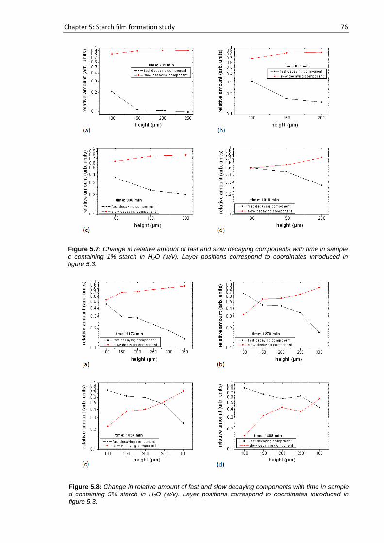
Chapter 5: Starch film formation study 76
Figure 5.7: Change in relative amount of fast and slow decaying components with time in sample c containing 1% starch in H2O (w/v). Layer positions correspond to coordinates introduced in figure 5.3.
Figure 5.8: Change in relative amount of fast and slow decaying components with time in sample d containing 5% starch in H2O (w/v). Layer positions correspond to coordinates introduced in figure 5.3.
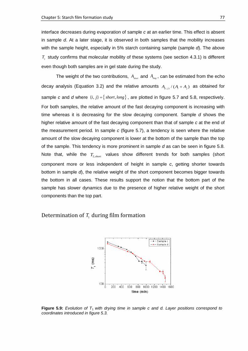
Chapter 5: Starch film formation study 77
interface decreases during evaporation of sample c at an earlier time. This effect is absent
in sample d. At a later stage, it is observed in both samples that the mobility increases
with the sample height, especially in 5% starch containing sample (sample d). The above
2T study confirms that molecular mobility of these systems (see section 4.3.1) is different
even though both samples are in gel state during the study.
The weight of the two contributions, short
A and longA , can be estimated from the echo
decay analysis (Equation 3.2) and the relative amounts ( , )
/ ( )i j i j
A A A as obtained for
sample c and d where { , } ,i j short long , are plotted in figure 5.7 and 5.8, respectively.
For both samples, the relative amount of the fast decaying component is increasing with
time whereas it is decreasing for the slow decaying component. Sample d shows the
higher relative amount of the fast decaying component than that of sample c at the end of
the measurement period. In sample c (figure 5.7), a tendency is seen where the relative
amount of the slow decaying component is lower at the bottom of the sample than the top
of the sample. This tendency is more prominent in sample d as can be seen in figure 5.8.
Note that, while the 2,shortT values show different trends for both samples (short
component more or less independent of height in sample c, getting shorter towards
bottom in sample d), the relative weight of the short component becomes bigger towards
the bottom in all cases. These results support the notion that the bottom part of the
sample has slower dynamics due to the presence of higher relative weight of the short
components than the top part.
Determination of 1T during film formation
Figure 5.9: Evolution of T1 with drying time in sample c and d. Layer positions correspond to coordinates introduced in figure 5.3.
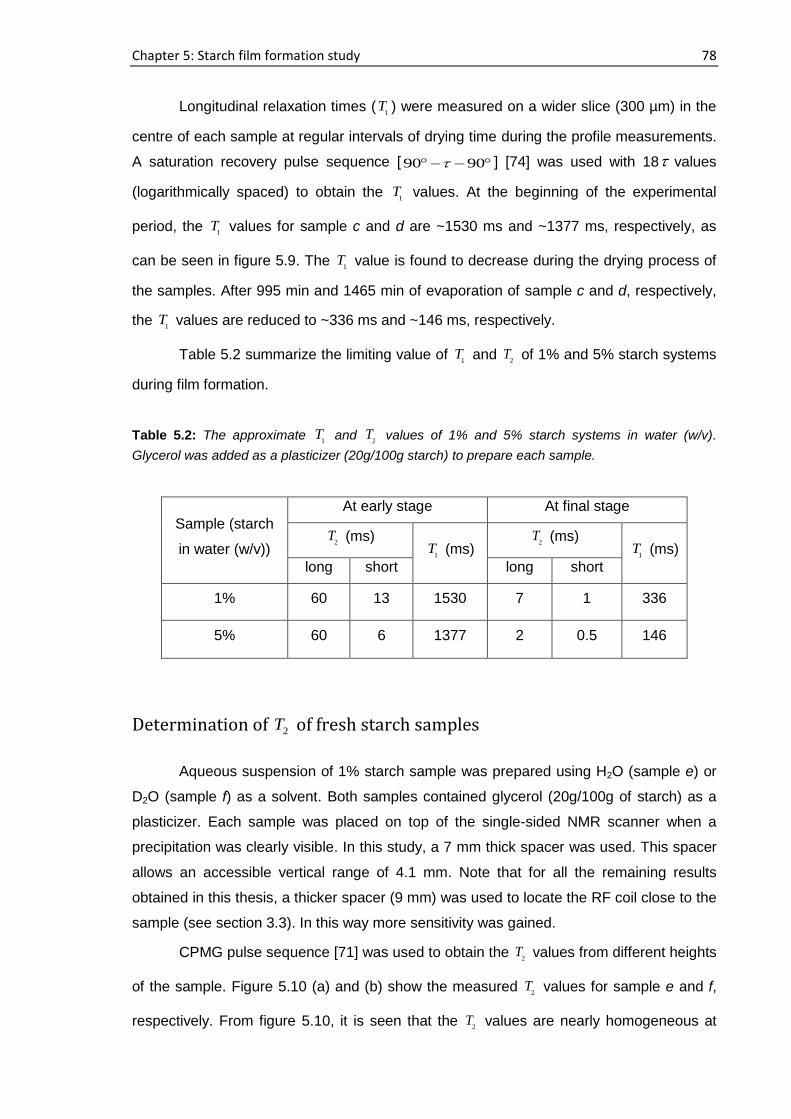
Chapter 5: Starch film formation study 78
Longitudinal relaxation times (1
T ) were measured on a wider slice (300 µm) in the
centre of each sample at regular intervals of drying time during the profile measurements.
A saturation recovery pulse sequence [ 90 90 ] [74] was used with 18 values
(logarithmically spaced) to obtain the 1
T values. At the beginning of the experimental
period, the 1
T values for sample c and d are ~1530 ms and ~1377 ms, respectively, as
can be seen in figure 5.9. The 1
T value is found to decrease during the drying process of
the samples. After 995 min and 1465 min of evaporation of sample c and d, respectively,
the 1
T values are reduced to ~336 ms and ~146 ms, respectively.
Table 5.2 summarize the limiting value of 1
T and 2
T of 1% and 5% starch systems
during film formation.
Table 5.2: The approximate 1
T and 2
T values of 1% and 5% starch systems in water (w/v).
Glycerol was added as a plasticizer (20g/100g starch) to prepare each sample.
Sample (starch
in water (w/v))
At early stage At final stage
2T (ms)
1T (ms)
2T (ms)
1T (ms)
long short long short
1% 60 13 1530 7 1 336
5% 60 6 1377 2 0.5 146
Determination of 2T of fresh starch samples
Aqueous suspension of 1% starch sample was prepared using H2O (sample e) or
D2O (sample f) as a solvent. Both samples contained glycerol (20g/100g of starch) as a
plasticizer. Each sample was placed on top of the single-sided NMR scanner when a
precipitation was clearly visible. In this study, a 7 mm thick spacer was used. This spacer
allows an accessible vertical range of 4.1 mm. Note that for all the remaining results
obtained in this thesis, a thicker spacer (9 mm) was used to locate the RF coil close to the
sample (see section 3.3). In this way more sensitivity was gained.
CPMG pulse sequence [71] was used to obtain the 2
T values from different heights
of the sample. Figure 5.10 (a) and (b) show the measured 2
T values for sample e and f,
respectively. From figure 5.10, it is seen that the 2
T values are nearly homogeneous at
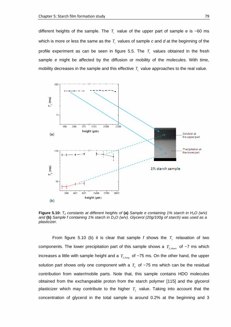
Chapter 5: Starch film formation study 79
different heights of the sample. The 2
T value of the upper part of sample e is ~60 ms
which is more or less the same as the 2
T values of sample c and d at the beginning of the
profile experiment as can be seen in figure 5.5. The 2
T values obtained in the fresh
sample e might be affected by the diffusion or mobility of the molecules. With time,
mobility decreases in the sample and this effective 2
T value approaches to the real value.
From figure 5.10 (b) it is clear that sample f shows the 2
T relaxation of two
components. The lower precipitation part of this sample shows a 2,shortT of ~7 ms which
increases a little with sample height and a 2,longT of ~75 ms. On the other hand, the upper
solution part shows only one component with a 2T of ~75 ms which can be the residual
contribution from water/mobile parts. Note that, this sample contains HDO molecules
obtained from the exchangeable proton from the starch polymer [115] and the glycerol
plasticizer which may contribute to the higher 2T value. Taking into account that the
concentration of glycerol in the total sample is around 0.2% at the beginning and 3
Figure 5.10: T2 constants at different heights of (a) Sample e containing 1% starch in H2O (w/v) and (b) Sample f containing 1% starch in D2O (w/v). Glycerol (20g/100g of starch) was used as a plasticizer.
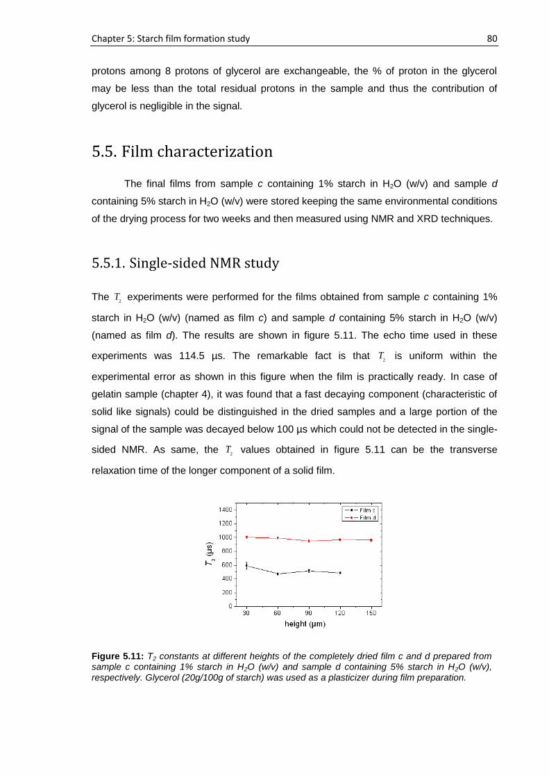
Chapter 5: Starch film formation study 80
protons among 8 protons of glycerol are exchangeable, the % of proton in the glycerol
may be less than the total residual protons in the sample and thus the contribution of
glycerol is negligible in the signal.
5.5. Film characterization
The final films from sample c containing 1% starch in H2O (w/v) and sample d
containing 5% starch in H2O (w/v) were stored keeping the same environmental conditions
of the drying process for two weeks and then measured using NMR and XRD techniques.
5.5.1. Single-sided NMR study
The 2
T experiments were performed for the films obtained from sample c containing 1%
starch in H2O (w/v) (named as film c) and sample d containing 5% starch in H2O (w/v)
(named as film d). The results are shown in figure 5.11. The echo time used in these
experiments was 114.5 µs. The remarkable fact is that 2
T is uniform within the
experimental error as shown in this figure when the film is practically ready. In case of
gelatin sample (chapter 4), it was found that a fast decaying component (characteristic of
solid like signals) could be distinguished in the dried samples and a large portion of the
signal of the sample was decayed below 100 µs which could not be detected in the single-
sided NMR. As same, the 2
T values obtained in figure 5.11 can be the transverse
relaxation time of the longer component of a solid film.
Figure 5.11: T2 constants at different heights of the completely dried film c and d prepared from sample c containing 1% starch in H2O (w/v) and sample d containing 5% starch in H2O (w/v), respectively. Glycerol (20g/100g of starch) was used as a plasticizer during film preparation.
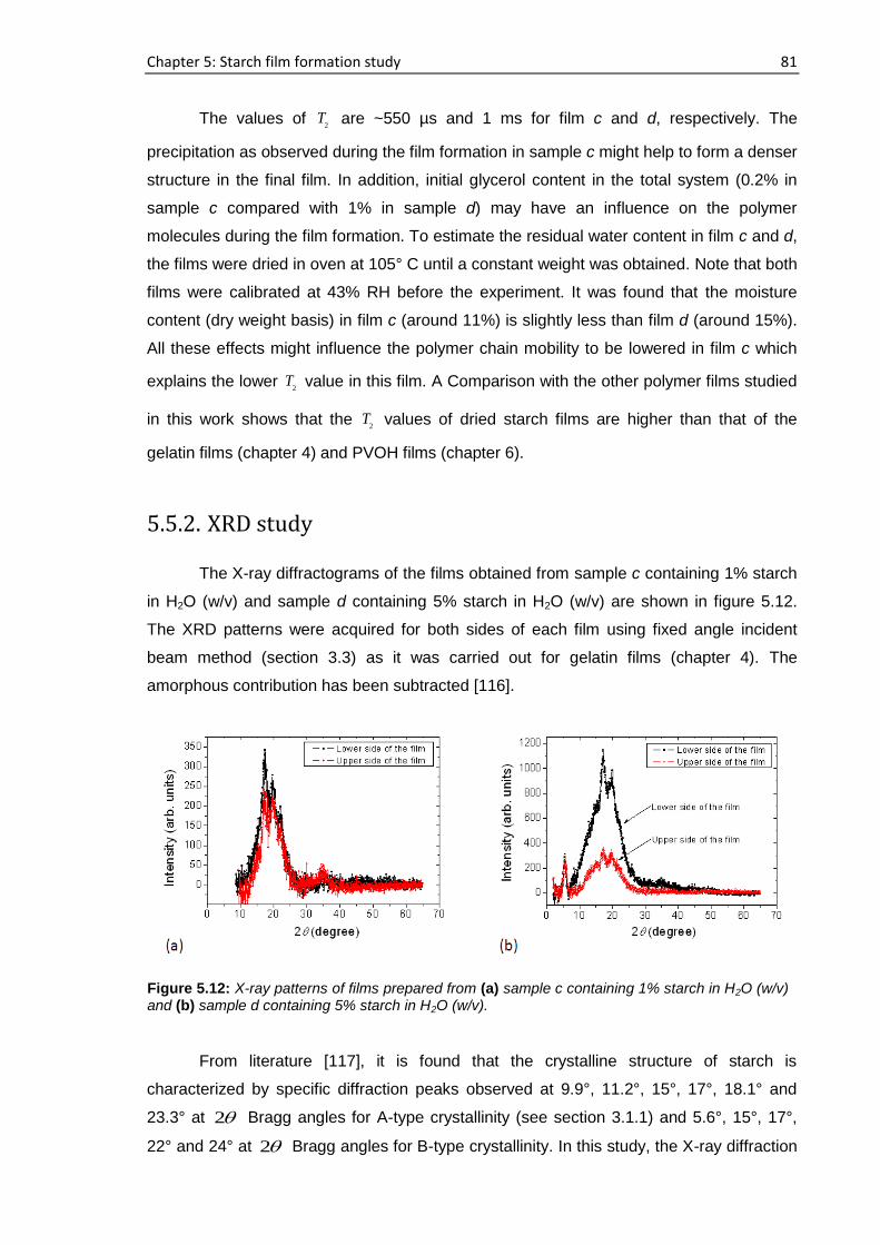
Chapter 5: Starch film formation study 81
The values of 2
T are ~550 µs and 1 ms for film c and d, respectively. The
precipitation as observed during the film formation in sample c might help to form a denser
structure in the final film. In addition, initial glycerol content in the total system (0.2% in
sample c compared with 1% in sample d) may have an influence on the polymer
molecules during the film formation. To estimate the residual water content in film c and d,
the films were dried in oven at 105° C until a constant weight was obtained. Note that both
films were calibrated at 43% RH before the experiment. It was found that the moisture
content (dry weight basis) in film c (around 11%) is slightly less than film d (around 15%).
All these effects might influence the polymer chain mobility to be lowered in film c which
explains the lower 2
T value in this film. A Comparison with the other polymer films studied
in this work shows that the 2
T values of dried starch films are higher than that of the
gelatin films (chapter 4) and PVOH films (chapter 6).
5.5.2. XRD study
The X-ray diffractograms of the films obtained from sample c containing 1% starch
in H2O (w/v) and sample d containing 5% starch in H2O (w/v) are shown in figure 5.12.
The XRD patterns were acquired for both sides of each film using fixed angle incident
beam method (section 3.3) as it was carried out for gelatin films (chapter 4). The
amorphous contribution has been subtracted [116].
From literature [117], it is found that the crystalline structure of starch is
characterized by specific diffraction peaks observed at 9.9°, 11.2°, 15°, 17°, 18.1° and
23.3° at 2 Bragg angles for A-type crystallinity (see section 3.1.1) and 5.6°, 15°, 17°,
22° and 24° at 2 Bragg angles for B-type crystallinity. In this study, the X-ray diffraction
Figure 5.12: X-ray patterns of films prepared from (a) sample c containing 1% starch in H2O (w/v) and (b) sample d containing 5% starch in H2O (w/v).
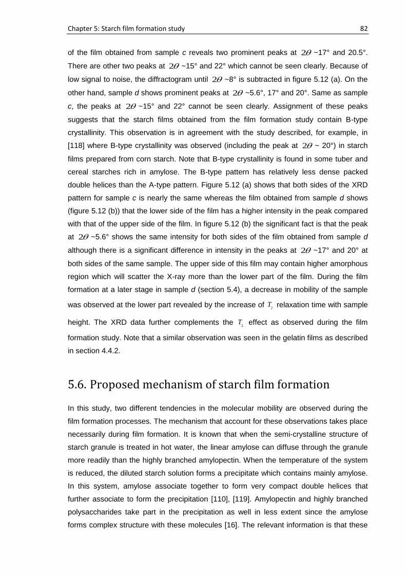
Chapter 5: Starch film formation study 82
of the film obtained from sample c reveals two prominent peaks at 2 ~17° and 20.5°.
There are other two peaks at 2 ~15° and 22° which cannot be seen clearly. Because of
low signal to noise, the diffractogram until 2 ~8° is subtracted in figure 5.12 (a). On the
other hand, sample d shows prominent peaks at 2 ~5.6°, 17° and 20°. Same as sample
c, the peaks at 2 ~15° and 22° cannot be seen clearly. Assignment of these peaks
suggests that the starch films obtained from the film formation study contain B-type
crystallinity. This observation is in agreement with the study described, for example, in
[118] where B-type crystallinity was observed (including the peak at 2 ~ 20°) in starch
films prepared from corn starch. Note that B-type crystallinity is found in some tuber and
cereal starches rich in amylose. The B-type pattern has relatively less dense packed
double helices than the A-type pattern. Figure 5.12 (a) shows that both sides of the XRD
pattern for sample c is nearly the same whereas the film obtained from sample d shows
(figure 5.12 (b)) that the lower side of the film has a higher intensity in the peak compared
with that of the upper side of the film. In figure 5.12 (b) the significant fact is that the peak
at 2 ~5.6° shows the same intensity for both sides of the film obtained from sample d
although there is a significant difference in intensity in the peaks at 2 ~17° and 20° at
both sides of the same sample. The upper side of this film may contain higher amorphous
region which will scatter the X-ray more than the lower part of the film. During the film
formation at a later stage in sample d (section 5.4), a decrease in mobility of the sample
was observed at the lower part revealed by the increase of 2
T relaxation time with sample
height. The XRD data further complements the 2
T effect as observed during the film
formation study. Note that a similar observation was seen in the gelatin films as described
in section 4.4.2.
5.6. Proposed mechanism of starch film formation
In this study, two different tendencies in the molecular mobility are observed during the
film formation processes. The mechanism that account for these observations takes place
necessarily during film formation. It is known that when the semi-crystalline structure of
starch granule is treated in hot water, the linear amylose can diffuse through the granule
more readily than the highly branched amylopectin. When the temperature of the system
is reduced, the diluted starch solution forms a precipitate which contains mainly amylose.
In this system, amylose associate together to form very compact double helices that
further associate to form the precipitation [110], [119]. Amylopectin and highly branched
polysaccharides take part in the precipitation as well in less extent since the amylose
forms complex structure with these molecules [16]. The relevant information is that these
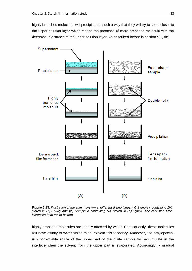
Chapter 5: Starch film formation study 83
highly branched molecules will precipitate in such a way that they will try to settle closer to
the upper solution layer which means the presence of more branched molecule with the
decrease in distance to the upper solution layer. As described before in section 5.1, the
highly branched molecules are readily affected by water. Consequently, these molecules
will have affinity to water which might explain this tendency. Moreover, the amylopectin-
rich non-volatile solute of the upper part of the dilute sample will accumulate in the
interface when the solvent from the upper part is evaporated. Accordingly, a gradual
Figure 5.13: Illustration of the starch system at different drying times. (a) Sample c containing 1% starch in H2O (w/v) and (b) Sample d containing 5% starch in H2O (w/v). The evolution time increases from top to bottom.
Chapter 5: Starch film formation study 84
increase in the amount of highly branched molecule near to the air-sample interface will
be established. The decrease in 2
T value towards the air-sample interface (figure 5.5 (a))
can be explained by the combination of these two occurrences. The starch sample
prepared from 5% starch in water is a gel from the beginning of film formation which does
not show this tendency.
At a later stage, a decrease in 2
T value at the bottom part of the sample can be
observed, especially in 5% starch containing sample. Starch gel consists of double helical
crystallite [16]. The crosslinked gel system is not stable due to continuous evaporation of
water. Consequently, it is most likely that the double helix structure precipitate when the
water concentration is reduced in the system presumable that the water takes part in the
structure making hydrogen bond. This process will reduce the mobility of the bottom part
of the sample which is possible to follow from the relaxation study. In this way, the
interplay of water evaporation and polymer migration result, for the conditions studied in
this work, in a dynamic heterogeneity of the polymer molecules across the film thickness,
which develops gradually after the average water concentration drops below a critical
value. The XRD data shows that the dense triple-helix structure that is preferably
generated at the bottom of the sample during the evaporation makes a significant
difference in the structure of the final film.
5.7. Conclusions
A number of studies were conducted to follow the evaporation of the solvent from
two different starch samples containing 1% and 5% of starch in water (w/v) during the
process of film formation. In both systems, glycerol was used as a plasticizer. These
studies enable one to understand the starch-H2O system at a molecular level. Using a
micro camera, evaporation of the solvent from these starch systems was observed
optically revealing that at the macroscopic level, the evaporation tendency of these two
systems is different. While 1% starch containing sample forms a precipitation at the
beginning, 5% starch containing sample is a gel. With evaporation, the thickness of the
upper solution part of 1% starch containing sample reduced due to solvent evaporation
and the lower precipitation layer became dense packed.
By a time-dependent NMR 1D-microimaging (profile) measurement of the samples
it was found that the transverse relaxation times (2
T ) represent a suitable measure for
indicating the residual mobility of the sample, whereas the signal intensity determined
along the profile requires taking the evolution of 1
T into account. The 1% starch containing
sample showed a gradual decrease in the mobility of the polymer molecules near to the
Chapter 5: Starch film formation study 85
air-sample interface at the beginning of the experiment period which was totally absent in
the sample containing 5% starch in water. When both starch samples were approaching
the final drying stage, the 2
T values of the system near the substrate decreased more
compared with that of the vicinity of the air-sample interface. Subsequent analysis of the
completely dried film by X-ray diffractometry revealed that the amorphous region at the
upper surface is indeed considerably higher than that at the lower surface. These
observations are similar to earlier finding obtained for gelatin solutions, where network
formation and precipitation resulted in an increased crystallinity at the bottom surface
(chapter 4).
In this chapter, the progress of molecular mobility of starch suspension until the
final stages of film drying has been investigated with spatial resolution for the first time by
using NMR relaxometry, providing insight into the development of resolved polymer
concentration. The main conclusion from the complete set of experiments is that the
starch film is drying in a stratified fashion.
86
Chapter 6
Structural and dynamical heterogeneities
of PVOH film during its formation
The opposite of a correct statement is a false statement.
But the opposite of a profound truth may well be another profound truth.
Niels Bohr
6.1. Introduction
Water is used as a common solvent for the production of semi-crystalline poly(vinyl
alcohol) (PVOH) film. Above the glass transition temperature ( 85
gT C ) fully hydrolyzed
PVOH is completely soluble in water [120]. The interaction between the PVOH and water
molecules plays an important role in polymer chain dynamics in the solution [121]. With
continuous evaporation of water this dynamic changes in time and the final film is
obtained from a cast solution. Films from PVOH in aqueous solution have been a largely
studied system, however, most of them refer to crosslinked hydrogels [120], [122]-[124].
The influence of the formation process in solution-based PVOH films shows different
characteristics; contrary to hydrogels, PVOH film formation by solvent evaporation does
not involve any cross-linking (gelation). However, a number of complex interactions are
still present making difficult any quantitative description accounting for the processes that
drive the cast solution to the final film. A number of references [11], [18]-[21] have been
devoted to study of the drying of the PVOH solution. There, a “skin” formation process has
been reported which consists of a glassy layer formation on top of the evaporating
solution. This process is related to the shifting of the glass transition temperature ( gT ) due
to the change in the solvent concentration. As the PVOH film is semicrystalline in nature,
Chapter 6: Structural and dynamical heterogeneities of PVOH film during its formation 87
the removal of solvent during the film formation process will drive both the crystallization
and the amorphous phase (glass) formation process. In particular the glass transition
temperature of the PVOH-water mixture will increase. As a consequence, a glassy layer
may develop in the air-sample interface as the solvent removal rate is faster in this part of
the sample, compared with the bulk solution system. On the other hand, the development
of a crystalline skin is reported in reference [22] on the basis of the change in evaporation
rate during the film formation. In this reference magnetic resonance imaging (MRI) studies
of PVOH cast from aqueous solution as a function of time show nonuniform water
distribution at certain drying conditions, coupled with a crystalline layer at the top surface
of the solution. However, detailed microscopic experimental studies explaining these
observations as well as the structural characterization of the final film addressing these
phenomena are scarce.
In this chapter, the presence of gradual heterogeneities in dynamics during film
formation of the PVOH in an aqueous solution is experimentally demonstrated using
single-sided NMR technique. X-ray diffraction (XRD) technique is used to study the film
which is capable of providing information on structure of the final state of the PVOH film at
a molecular level. The NMR studies presented here reveal a progressive process leading
to a hardening of the top regions of the film assessed by the relaxation times 2
T and 1
T
gradually growing towards the bottom part of the sample. Beside the single-sided NMR
scanner, a Minispec and a field cycling relaxometer are used to study the 2
T and 1
T ,
respectively to obtain additional information. The heterogeneity identified by the NMR
study is confirmed by the XRD study of the film. In this way, dynamic and structural
studies performed with NMR and XRD, respectively, provide evidence that
heterogeneities in the film formation process and in the final film are present.
6.2. Samples
Table 6.1 shows the characteristics of the samples used in this work. The film
formation of PVOH of three different molecular weights, MW=27000 (indicated as 27K),
61000 (61K) and 125000 (125K) was investigated in order to observe the molecular
weight dependency. While most of the experiments were carried out with the sample of
61K (sample a, c, e, f, g, h and i), comparative measurements were repeated under
similar experimental conditions for 27K (sample b) and 125K (sample d), respectively.
Deuterated water (D2O) was used as a solvent (sample a, e, g and i) in order to selectively
follow the dynamics of the backbone of the PVOH molecules. The results obtained using
H2O as a solvent were compared with those obtained using D2O. The initial concentration

Chapter 6: Structural and dynamical heterogeneities of PVOH film during its formation 88
of PVOH in the solution was set to 25% (w/v) for all the samples. The same protocol was
used for the preparation of all the samples to be diluted either with H2O or D2O. Note that
when PVOH is used as a hydrogel, the gel is induced only after several cycles of a
freezing-thawing process [125], [126]. However, no gel formation was observed after
several hours of preparation in the present work.
Table 6.1: Different PVOH samples prepared using H2O or D2O as a solvent. The initial concentration of PVOH in solution was 25% (w/v).
Sample Molecular weight
of PVOH
Solvent Study Thickness of the
final film (µm)
a 61K D2O Profiling at 11.7 MHz
(1H) and XRD 275 ± 10
b 27K H2O Profiling at 11.7 MHz
(1H) and XRD 380 ± 25
c 61K H2O Profiling at 11.7 MHz
(1H) and XRD 340 ± 12
d 125K H2O Profiling at 11.7 MHz
(1H) and XRD 268 ± 15
e 61K D2O 1
T at 11.7 MHz (1H) ---
f 61K H2O Diffusion at 11.7 MHz
(1H) ---
g 61K D2O Diffusion at 11.7 MHz
(1H) ---
h 61K H2O 1T and
2T at 40 MHz
(1H)
---
i 61K D2O 1T and
2T at 40 MHz
(1H) ---
For the diffusion measurements, sample f (25% (w/v) PVOH in H2O) and sample g
(25% (w/v) PVOH in D2O) were prepared and the stimulated echo sequence in
combination with the static magnetic field gradient of the sensor was used. The
measurements were performed right after the casting, sealing the container to avoid
evaporation. For this measurement an encoding time = 0.0055 to 1.9 ms, diffusion time
= 2 ms, repetition time of 3 s and 5 s (for sample f and g, respectively) were used. All
experiments were performed at room temperature.
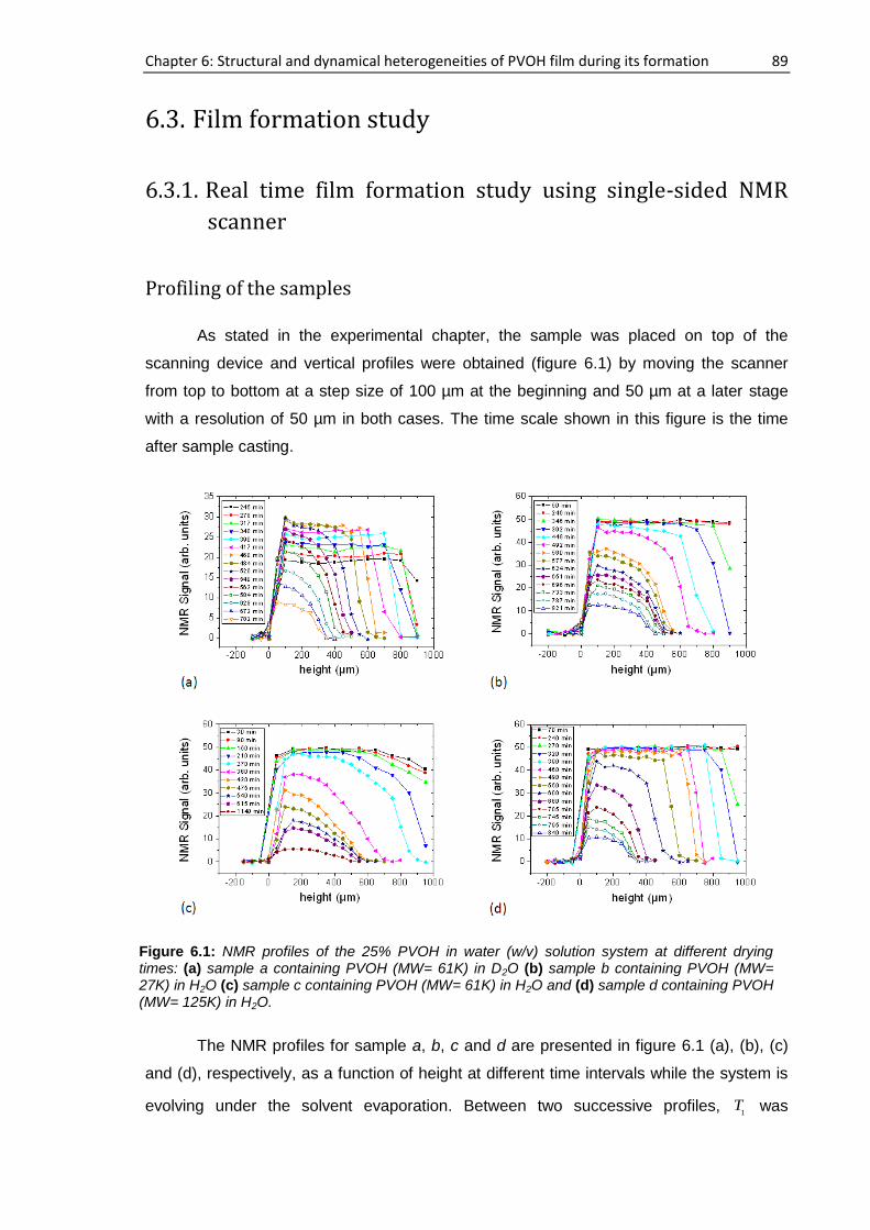
Chapter 6: Structural and dynamical heterogeneities of PVOH film during its formation 89
6.3. Film formation study
6.3.1. Real time film formation study using single-sided NMR
scanner
Profiling of the samples
As stated in the experimental chapter, the sample was placed on top of the
scanning device and vertical profiles were obtained (figure 6.1) by moving the scanner
from top to bottom at a step size of 100 µm at the beginning and 50 µm at a later stage
with a resolution of 50 µm in both cases. The time scale shown in this figure is the time
after sample casting.
The NMR profiles for sample a, b, c and d are presented in figure 6.1 (a), (b), (c)
and (d), respectively, as a function of height at different time intervals while the system is
evolving under the solvent evaporation. Between two successive profiles, 1
T was
Figure 6.1: NMR profiles of the 25% PVOH in water (w/v) solution system at different drying times: (a) sample a containing PVOH (MW= 61K) in D2O (b) sample b containing PVOH (MW= 27K) in H2O (c) sample c containing PVOH (MW= 61K) in H2O and (d) sample d containing PVOH (MW= 125K) in H2O.
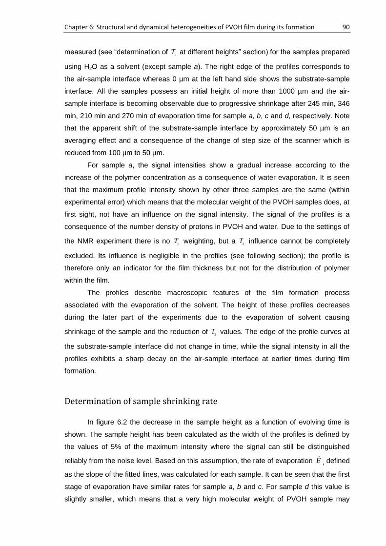
Chapter 6: Structural and dynamical heterogeneities of PVOH film during its formation 90
measured (see “determination of 1
T at different heights” section) for the samples prepared
using H2O as a solvent (except sample a). The right edge of the profiles corresponds to
the air-sample interface whereas 0 µm at the left hand side shows the substrate-sample
interface. All the samples possess an initial height of more than 1000 µm and the air-
sample interface is becoming observable due to progressive shrinkage after 245 min, 346
min, 210 min and 270 min of evaporation time for sample a, b, c and d, respectively. Note
that the apparent shift of the substrate-sample interface by approximately 50 µm is an
averaging effect and a consequence of the change of step size of the scanner which is
reduced from 100 µm to 50 µm.
For sample a, the signal intensities show a gradual increase according to the
increase of the polymer concentration as a consequence of water evaporation. It is seen
that the maximum profile intensity shown by other three samples are the same (within
experimental error) which means that the molecular weight of the PVOH samples does, at
first sight, not have an influence on the signal intensity. The signal of the profiles is a
consequence of the number density of protons in PVOH and water. Due to the settings of
the NMR experiment there is no 1
T weighting, but a 2
T influence cannot be completely
excluded. Its influence is negligible in the profiles (see following section); the profile is
therefore only an indicator for the film thickness but not for the distribution of polymer
within the film.
The profiles describe macroscopic features of the film formation process
associated with the evaporation of the solvent. The height of these profiles decreases
during the later part of the experiments due to the evaporation of solvent causing
shrinkage of the sample and the reduction of 2
T values. The edge of the profile curves at
the substrate-sample interface did not change in time, while the signal intensity in all the
profiles exhibits a sharp decay on the air-sample interface at earlier times during film
formation.
Determination of sample shrinking rate
In figure 6.2 the decrease in the sample height as a function of evolving time is
shown. The sample height has been calculated as the width of the profiles is defined by
the values of 5% of the maximum intensity where the signal can still be distinguished
reliably from the noise level. Based on this assumption, the rate of evaporation E , defined
as the slope of the fitted lines, was calculated for each sample. It can be seen that the first
stage of evaporation have similar rates for sample a, b and c. For sample d this value is
slightly smaller, which means that a very high molecular weight of PVOH sample may
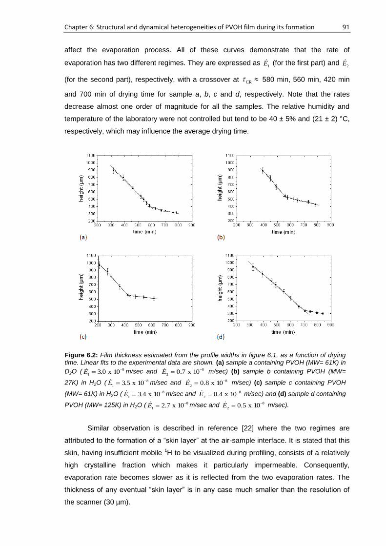
Chapter 6: Structural and dynamical heterogeneities of PVOH film during its formation 91
affect the evaporation process. All of these curves demonstrate that the rate of
evaporation has two different regimes. They are expressed as 1E (for the first part) and
2E
(for the second part), respectively, with a crossover at CR 580 min, 560 min, 420 min
and 700 min of drying time for sample a, b, c and d, respectively. Note that the rates
decrease almost one order of magnitude for all the samples. The relative humidity and
temperature of the laboratory were not controlled but tend to be 40 ± 5% and (21 ± 2) °C,
respectively, which may influence the average drying time.
Similar observation is described in reference [22] where the two regimes are
attributed to the formation of a “skin layer” at the air-sample interface. It is stated that this
skin, having insufficient mobile 1H to be visualized during profiling, consists of a relatively
high crystalline fraction which makes it particularly impermeable. Consequently,
evaporation rate becomes slower as it is reflected from the two evaporation rates. The
thickness of any eventual “skin layer” is in any case much smaller than the resolution of
the scanner (30 µm).
Figure 6.2: Film thickness estimated from the profile widths in figure 6.1, as a function of drying time. Linear fits to the experimental data are shown. (a) sample a containing PVOH (MW= 61K) in
D2O ( 8
13.0 x 10
E m/sec and 8
20.7 x 10
E m/sec) (b) sample b containing PVOH (MW=
27K) in H2O ( 8
13.5 x 10
E m/sec and 8
20.8 x 10
E m/sec) (c) sample c containing PVOH
(MW= 61K) in H2O ( 8
13.4 x 10
E m/sec and 8
20.4 x 10
E m/sec) and (d) sample d containing
PVOH (MW= 125K) in H2O ( 8
12.7 x 10
E m/sec and 8
20.5 x 10
E m/sec).
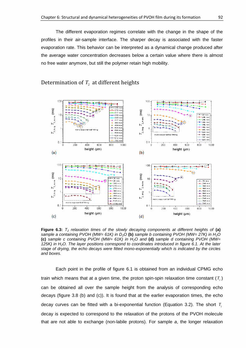
Chapter 6: Structural and dynamical heterogeneities of PVOH film during its formation 92
The different evaporation regimes correlate with the change in the shape of the
profiles in their air-sample interface. The sharper decay is associated with the faster
evaporation rate. This behavior can be interpreted as a dynamical change produced after
the average water concentration decreases below a certain value where there is almost
no free water anymore, but still the polymer retain high mobility.
Determination of 2T at different heights
Each point in the profile of figure 6.1 is obtained from an individual CPMG echo
train which means that at a given time, the proton spin-spin relaxation time constant (2
T )
can be obtained all over the sample height from the analysis of corresponding echo
decays (figure 3.8 (b) and (c)). It is found that at the earlier evaporation times, the echo
decay curves can be fitted with a bi-exponential function (Equation 3.2). The short 2
T
decay is expected to correspond to the relaxation of the protons of the PVOH molecule
that are not able to exchange (non-labile protons). For sample a, the longer relaxation
Figure 6.3: T2 relaxation times of the slowly decaying components at different heights of (a) sample a containing PVOH (MW= 61K) in D2O (b) sample b containing PVOH (MW= 27K) in H2O (c) sample c containing PVOH (MW= 61K) in H2O and (d) sample d containing PVOH (MW= 125K) in H2O. The layer positions correspond to coordinates introduced in figure 6.1. At the later stage of drying, the echo decays were fitted mono-exponentially which is indicated by the circles and boxes.
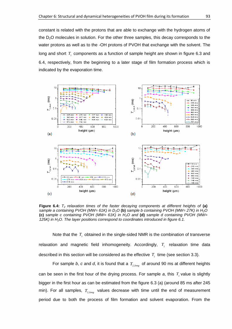
Chapter 6: Structural and dynamical heterogeneities of PVOH film during its formation 93
constant is related with the protons that are able to exchange with the hydrogen atoms of
the D2O molecules in solution. For the other three samples, this decay corresponds to the
water protons as well as to the -OH protons of PVOH that exchange with the solvent. The
long and short 2
T components as a function of sample height are shown in figure 6.3 and
6.4, respectively, from the beginning to a later stage of film formation process which is
indicated by the evaporation time.
Note that the 2
T obtained in the single-sided NMR is the combination of transverse
relaxation and magnetic field inhomogeneity. Accordingly, 2
T relaxation time data
described in this section will be considered as the effective 2
T time (see section 3.3).
For sample b, c and d, it is found that a 2,longT of around 90 ms at different heights
can be seen in the first hour of the drying process. For sample a, this 2
T value is slightly
bigger in the first hour as can be estimated from the figure 6.3 (a) (around 85 ms after 245
min). For all samples, 2,longT values decrease with time until the end of measurement
period due to both the process of film formation and solvent evaporation. From the
Figure 6.4: T2 relaxation times of the faster decaying components at different heights of (a) sample a containing PVOH (MW= 61K) in D2O (b) sample b containing PVOH (MW= 27K) in H2O (c) sample c containing PVOH (MW= 61K) in H2O and (d) sample d containing PVOH (MW= 125K) in H2O. The layer positions correspond to coordinates introduced in figure 6.1.

Chapter 6: Structural and dynamical heterogeneities of PVOH film during its formation 94
relaxation behavior of the bottom part of the sample, it is also evident that the 2,longT
values decrease around two orders of magnitude (~90 ms to ~2 ms) during the drying
period. Figure 6.4 shows that 2,shortT is around 10 ms after first few hours of casting for
each sample which is decreased to around 0.1 ms until the short components are not
anymore detectable. Therefore, similar to the long components, 2,shortT decreases nearly
two orders of magnitude and then become undetectable by the experimental setup.
The fundamental observation in these figures is that the 2
T relaxation times
change at different layers for each measurement. From a certain time of evaporation
onwards (460, 492, 360 and 490 min for sample a, b, c and d, respectively), the echo
decay of the air-sample interface layer in all the samples, could only be fitted with a mono-
exponential function (Equation 3.1) to obtain the corresponding 2
T value (see figure 6.3).
For further evaporation times this feature extends on inner layers and at the end on the
complete sample. It can be seen that after 921, 1140 and 840 min for sample b, c, and d,
respectively, there is no second component all through the sample height as shown in the
last profile experiment in each sample. Note that the pulse separation used in these
experiments is 87.5 µs which means the first echo is generated after this time. The solid
like component, which decays within 100 µs [87], will be difficult to observe. This is the
reason why only one component is observed at the later stage of drying which indicates
the formation of a solid-like structure at the top surface of the sample. In figure 6.4 it is
also observed that 2
T values of the short components gradually decreases as the height
of the sample increases at later stage of evaporation time i.e. both long and short
components behave qualitatively in the same way. The values of 2
T do not show any
dependence on height at the beginning of the experiment indicating that at the beginning
of the film formation process, the solution is uniform. Note that for sample a, which is used
to follow the relaxation behaviour of the polymer chain, same type of 2
T dependency as a
function of sample height is observed. Furthermore, the short 2
T values of this sample are
similar to the shorter 2
T of sample b, c and d. The short 2
T values of the samples a, b, c
and d at the respective evolution time show very weak dependence on height inside the
experimental errors. At later times, the short components are not anymore detected. The
difference in gradual change of 2
T all along the layers in different experiments due to the
drying effects are bigger than any change in 2
T that could happen in the time taken for a
single profile. The relative difference between the maximum and minimum 2
T (calculated
from the bottom and the top surface of the sample, respectively) comparing to 2
T of the
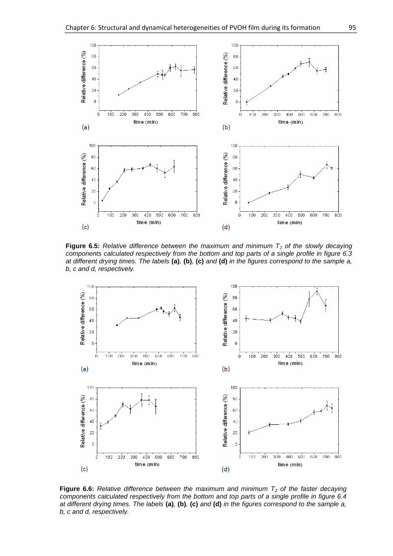
Chapter 6: Structural and dynamical heterogeneities of PVOH film during its formation 95
Figure 6.5: Relative difference between the maximum and minimum T2 of the slowly decaying components calculated respectively from the bottom and top parts of a single profile in figure 6.3 at different drying times. The labels (a), (b), (c) and (d) in the figures correspond to the sample a, b, c and d, respectively.
Figure 6.6: Relative difference between the maximum and minimum T2 of the faster decaying components calculated respectively from the bottom and top parts of a single profile in figure 6.4 at different drying times. The labels (a), (b), (c) and (d) in the figures correspond to the sample a, b, c and d, respectively.
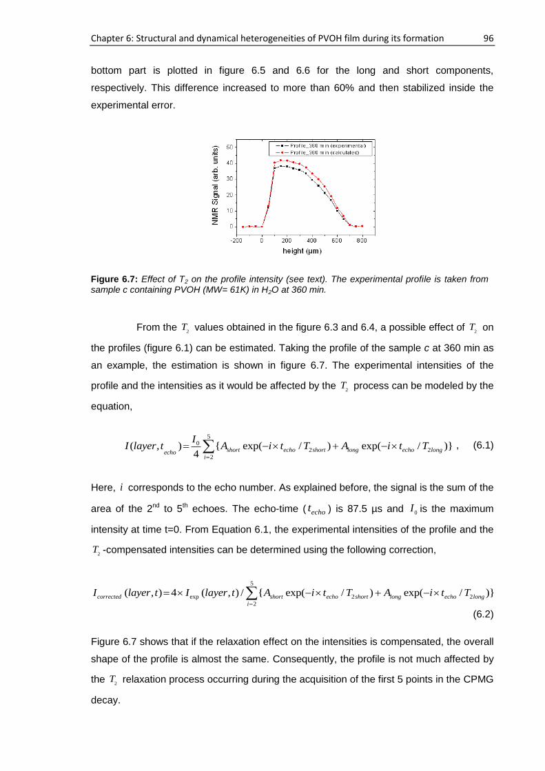
Chapter 6: Structural and dynamical heterogeneities of PVOH film during its formation 96
bottom part is plotted in figure 6.5 and 6.6 for the long and short components,
respectively. This difference increased to more than 60% and then stabilized inside the
experimental error.
From the 2
T values obtained in the figure 6.3 and 6.4, a possible effect of 2
T on
the profiles (figure 6.1) can be estimated. Taking the profile of the sample c at 360 min as
an example, the estimation is shown in figure 6.7. The experimental intensities of the
profile and the intensities as it would be affected by the 2
T process can be modeled by the
equation,
5
02 2
2
( , ) { exp( / ) exp( / )}4
short echo short long echo long
iecho
II layer t A i t T A i t T , (6.1)
Here, i corresponds to the echo number. As explained before, the signal is the sum of the
area of the 2nd to 5th echoes. The echo-time ( echot ) is 87.5 µs and 0I is the maximum
intensity at time t=0. From Equation 6.1, the experimental intensities of the profile and the
2T -compensated intensities can be determined using the following correction,
5
exp 2 2
2
( , ) 4 ( , ) / { exp( / ) exp( / )}
corrected short echo short long echo long
i
I layer t I layer t A i t T A i t T
(6.2)
Figure 6.7 shows that if the relaxation effect on the intensities is compensated, the overall
shape of the profile is almost the same. Consequently, the profile is not much affected by
the 2
T relaxation process occurring during the acquisition of the first 5 points in the CPMG
decay.
Figure 6.7: Effect of T2 on the profile intensity (see text). The experimental profile is taken from sample c containing PVOH (MW= 61K) in H2O at 360 min.
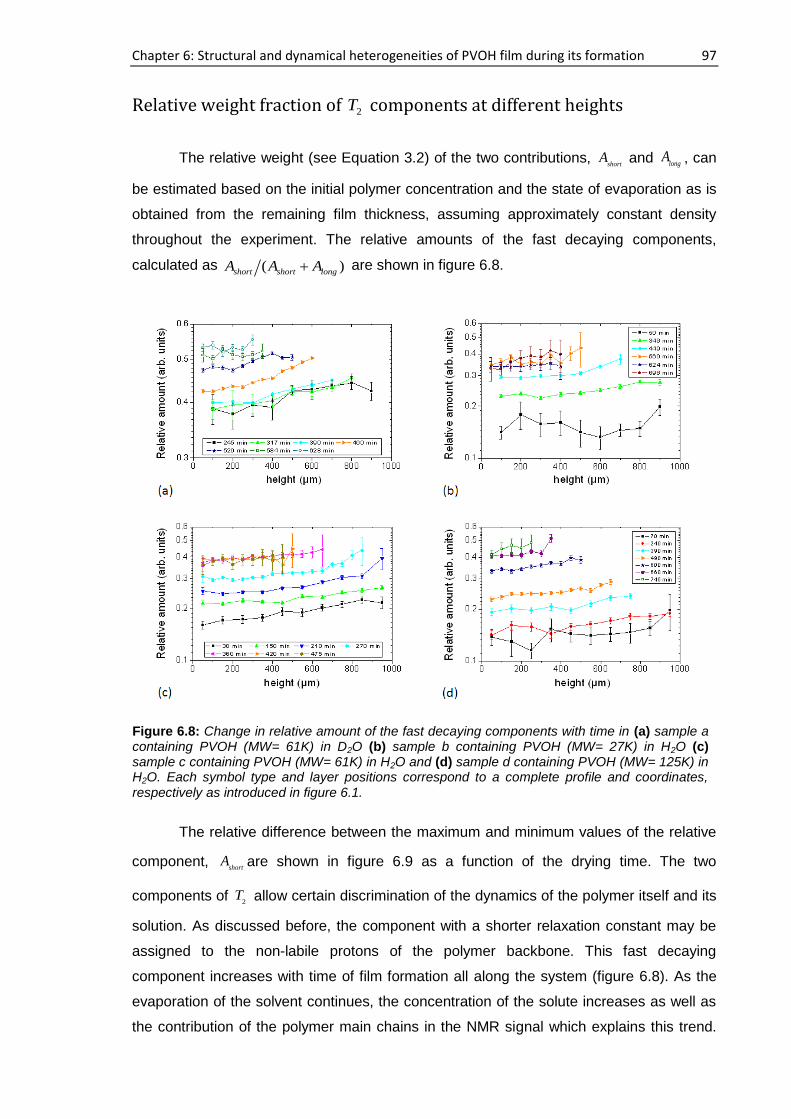
Chapter 6: Structural and dynamical heterogeneities of PVOH film during its formation 97
Relative weight fraction of 2T components at different heights
The relative weight (see Equation 3.2) of the two contributions, short
A and longA , can
be estimated based on the initial polymer concentration and the state of evaporation as is
obtained from the remaining film thickness, assuming approximately constant density
throughout the experiment. The relative amounts of the fast decaying components,
calculated as ( )short short longA A A are shown in figure 6.8.
The relative difference between the maximum and minimum values of the relative
component, short
A are shown in figure 6.9 as a function of the drying time. The two
components of 2
T allow certain discrimination of the dynamics of the polymer itself and its
solution. As discussed before, the component with a shorter relaxation constant may be
assigned to the non-labile protons of the polymer backbone. This fast decaying
component increases with time of film formation all along the system (figure 6.8). As the
evaporation of the solvent continues, the concentration of the solute increases as well as
the contribution of the polymer main chains in the NMR signal which explains this trend.
Figure 6.8: Change in relative amount of the fast decaying components with time in (a) sample a containing PVOH (MW= 61K) in D2O (b) sample b containing PVOH (MW= 27K) in H2O (c) sample c containing PVOH (MW= 61K) in H2O and (d) sample d containing PVOH (MW= 125K) in H2O. Each symbol type and layer positions correspond to a complete profile and coordinates, respectively as introduced in figure 6.1.
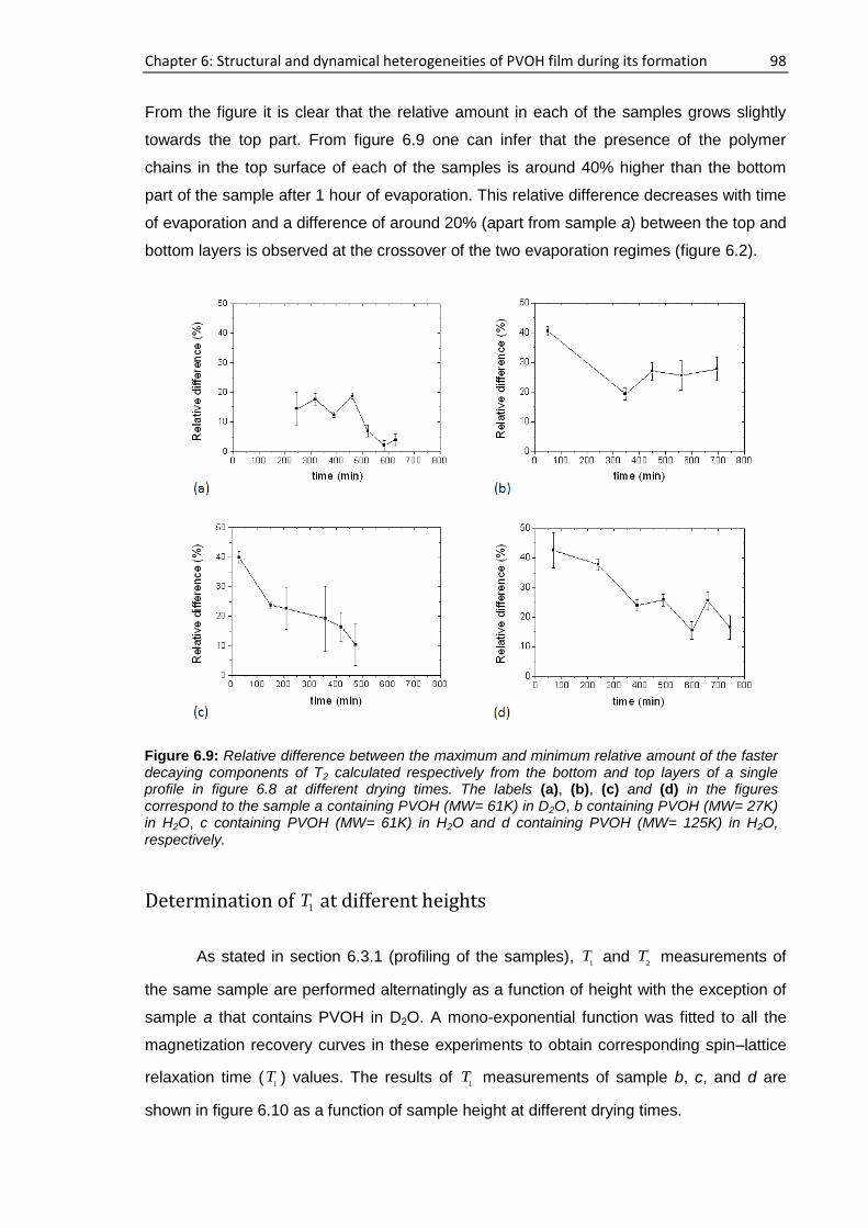
Chapter 6: Structural and dynamical heterogeneities of PVOH film during its formation 98
From the figure it is clear that the relative amount in each of the samples grows slightly
towards the top part. From figure 6.9 one can infer that the presence of the polymer
chains in the top surface of each of the samples is around 40% higher than the bottom
part of the sample after 1 hour of evaporation. This relative difference decreases with time
of evaporation and a difference of around 20% (apart from sample a) between the top and
bottom layers is observed at the crossover of the two evaporation regimes (figure 6.2).
Determination of 1T at different heights
As stated in section 6.3.1 (profiling of the samples), 1
T and 2
T measurements of
the same sample are performed alternatingly as a function of height with the exception of
sample a that contains PVOH in D2O. A mono-exponential function was fitted to all the
magnetization recovery curves in these experiments to obtain corresponding spin–lattice
relaxation time (1
T ) values. The results of 1
T measurements of sample b, c, and d are
shown in figure 6.10 as a function of sample height at different drying times.
Figure 6.9: Relative difference between the maximum and minimum relative amount of the faster decaying components of T2 calculated respectively from the bottom and top layers of a single profile in figure 6.8 at different drying times. The labels (a), (b), (c) and (d) in the figures correspond to the sample a containing PVOH (MW= 61K) in D2O, b containing PVOH (MW= 27K) in H2O, c containing PVOH (MW= 61K) in H2O and d containing PVOH (MW= 125K) in H2O, respectively.

Chapter 6: Structural and dynamical heterogeneities of PVOH film during its formation 99
For sample a, the required number of scans was higher to obtain an acceptable
signal to noise ratio comparing to that of H2O containing samples during the CPMG
experiments. As a result, 1
T and 2
T measurements of this sample could not be carried out
alternatingly. A separate sample named e was prepared using D2O and magnetization
Figure 6.10: Evolution of T1 with drying time in (a) sample b containing PVOH (MW= 27K) in H2O (b) sample c containing PVOH (MW= 61K) in H2O and (c) sample d containing PVOH (MW= 125K) in H2O. The layer positions correspond to coordinates introduced in figure 6.1.
Figure 6.11: Evolution of T1 with drying time in sample e containing PVOH (MW= 61K) in D2O: (a) T1 of the long components and (b) T1 of the short components. At the later stage of drying, the magnetization recovery were fitted mono-exponentially which is indicated by the circles.
Chapter 6: Structural and dynamical heterogeneities of PVOH film during its formation 100
recovery data were obtained using same parameters and conditions. In this study, two
components were found and a bi-exponential function was fitted accordingly. The results
for sample e are shown in figure 6.11.
The 1T values of all the samples show common features. For instance,
1T values
decrease as a function of time as a result of the solvent evaporation. From figure 6.10, it
can be seen that starting from the three different 1
T values, 700 ms, 500 ms and 900 ms
for the sample b, c and d, respectively, all the samples show a minimum value of around
30 ms after evolution. In the general case, the NMR relaxation rate of polymers in solution
is proportional to the so-called segmental reorientation time [127], [128]
2
1
1 Hs
B
b a
T k T
, (6.3)
where b is the Kuhn segment length, Ha is the hydrodynamic radius of the segments and
is the viscosity of the medium surrounding the segment. T is the absolute temperature
and k
B is the Boltzmann constant. As the evaporation takes place, the mobility of the
polymer chains decreases due to the increase in the viscosity of the solution and as a
consequence, the NMR relaxation process is affected. In the case of pure water, 1
T and
2T have an inverse dependence with the viscosity as well [32], but this dependence not
necessarily holds for the case of water in a polymer-water solution.
After 1380 min, 2700 min and 1590 min of drying time, 1
T values of the sample b,
c and d, respectively, show a relative increase. It is expected that the crystalline
component in a solid polymer will have longer 1
T relaxation time than the corresponding
amorphous component at the same temperature and magnetic field [32]. The gradual
increase of 1
T towards the top of the solution at 1590 min in sample d is compatible with
the presence of more crystalline component in the top of the film. Before the minimum 1
T
is reached, the bottom parts of all the samples show longer 1
T than the corresponding
upper part following similar spatial patterns than 2
T along the height of the film. The
different values of 1
T along the sample height provide additional evidence that the drying
of the PVOH film is inhomogeneous. This effect is less pronounced in the short
component of sample e due to larger experimental error (figure 6.11 (b)). The weight
fraction of the two 2
T components of this sample does not show any particular trend.

Chapter 6: Structural and dynamical heterogeneities of PVOH film during its formation 101
Diffusion Study
The steady strong gradient of the single-sided NMR scanner was used to perform
the diffusion experiments. Figure 6.12 shows the echo decays of two freshly prepared
sample f and g where H2O and D2O are used as the solvent, respectively. The signal of
the residual 1H in the solvent from the sample g is strongly suppressed by a repetition time
much shorter than the corresponding 1
T . In this figure, two components can clearly be
distinguished. The diffusion attenuation for the two components in the slow-limit exchange
can be written as [44]
2 1 2 1
2 2exp expdiff short short long long
short short long long
A A KD A KDT T T T
,
(6.4)
where 2 2
3K G
. , ,G and represent gyromagnetic ratio of protons,
gradient strength, encoding time and diffusion time, respectively. Note that for sample f
and g, both conditions,2T and
1T are satisfied. As a result these two relaxation
times will not affect the diffusion measurement.
The values of the slow diffusion component corresponding to the polymer are (3.2
± 0.1) × 10-11 m2/s and (1.8 ± 0.4) × 10-11 m2/s for the sample f and g, respectively (Figure
6.12). On the other hand, the fast diffusion coefficient reflects the exchange of protons
between the backbone and the solvent. Sample f has a fast diffusion coefficient of (1.1 ±
0.1) × 10-9 m2/s while for sample g the value is (0.94 ± 0.06) × 10-9 m2/s. Both diffusion
coefficients are almost half the value of bulk water, a consequence of the high viscosity of
Figure 6.12: Stimulated echo decay curves of (a) sample f containing PVOH (MW= 61K) in H2O and (b) sample g containing PVOH (MW= 61K) in D2O measured in the single-sided NMR scanner right after the sample preparation. The solid lines are bi-exponential fittings to the experimental data.
Chapter 6: Structural and dynamical heterogeneities of PVOH film during its formation 102
the solution. Note that the water molecules in the PVOH aqueous solution exchange with
the hydroxyl groups of the polymer chain. The relative amount of free (or bulk) water is
found after a complete hydration of the PVOH molecules to be about 30 wt% in the
solution [120]. At the initial concentration, the sample has enough bulk water to dominate
the diffusion process.
The diffusion process is playing an important role in the understanding of the
heterogeneities in the dynamics observed during film formation. When the rate of
evaporation of the solvent is higher than a certain value, the solute-solvent distribution in
the solution system is not homogeneous. In order to have a quantitative insight, an
analysis similar to that stated in reference [22] can be made computing the relation
between the rate of the vertical convection and the diffusion of the polymer molecules:
E
D
, (6.5)
here is the layer thickness, E is the value of the thickness change as shown in figure
6.2 in m/s and D is the diffusion coefficient of the polymer molecules. When 1 ,
diffusion dominates in the solution and the film remain homogeneous throughout. For the
cases when 1 , the difference in concentration cannot be compensated by diffusion,
giving rise to a higher polymer concentration in the upper part of the solution. Taking the
values of 1E from figure 6.2 (c) and (a), one obtains 1.05 and 1.7 for the sample f and
g, respectively. This means that drying is taking place in a so-called heterogeneous
regime.
6.3.2. NMR study at 40 MHz
1T and
2T of freshly prepared PVOH solutions using H2O and D2O (labeled as
sample h and i, respectively) are studied at 40 MHz 1H Larmor frequency. Table 6.2
shows 1
T and 2
T , respectively, for both short and long components. From the table it is
seen that both samples prepared using H2O and D2O show two components while in the
single-sided NMR scanner at 11.7 MHz shows only one component during 2
T study as
described before. 1
T of the single component of the PVOH solution prepared using H2O at
11.7 MHz has to be compared with the long 1
T component at 40 MHz. The 1
T values of
the short component are 41 ms and 50 ms for the sample h and i, respectively, whereas
those are 668 ms and 1115 ms for the long components, respectively. It is seen that the
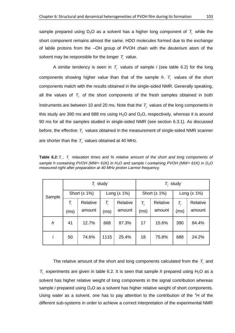
Chapter 6: Structural and dynamical heterogeneities of PVOH film during its formation 103
sample prepared using D2O as a solvent has a higher long component of 1
T while the
short component remains almost the same. HDO molecules formed due to the exchange
of labile protons from the –OH group of PVOH chain with the deuterium atom of the
solvent may be responsible for the longer 1
T value.
A similar tendency is seen in 2
T values of sample i (see table 6.2) for the long
components showing higher value than that of the sample h. 2
T values of the short
components match with the results obtained in the single-sided NMR. Generally speaking,
all the values of 2
T of the short components of the fresh samples obtained in both
instruments are between 10 and 20 ms. Note that the 2
T values of the long components in
this study are 390 ms and 688 ms using H2O and D2O, respectively, whereas it is around
90 ms for all the samples studied in single-sided NMR (see section 6.3.1). As discussed
before, the effective 2
T values obtained in the measurement of single-sided NMR scanner
are shorter than the 2
T values obtained at 40 MHz.
Table 6.2:1
T , 2
T relaxation times and % relative amount of the short and long components of
sample h containing PVOH (MW= 61K) in H2O and sample i containing PVOH (MW= 61K) in D2O measured right after preparation at 40 MHz proton Larmor frequency.
Sample
1T study
2T study
Short (± 1%) Long (± 1%) Short (± 1%) Long (± 1%)
1T
(ms)
Relative
amount
1T
(ms)
Relative
amount
2T
(ms)
Relative
amount
2T
(ms)
Relative
amount
h 41 12.7% 668 87.3% 17 15.6% 390 84.4%
i 50 74.6% 1115 25.4% 18 75.8% 688 24.2%
The relative amount of the short and long components calculated from the 1
T and
2T experiments are given in table 6.2. It is seen that sample h prepared using H2O as a
solvent has higher relative weight of long components in the signal contribution whereas
sample i prepared using D2O as a solvent has higher relative weight of short components.
Using water as a solvent, one has to pay attention to the contribution of the 1H of the
different sub-systems in order to achieve a correct interpretation of the experimental NMR
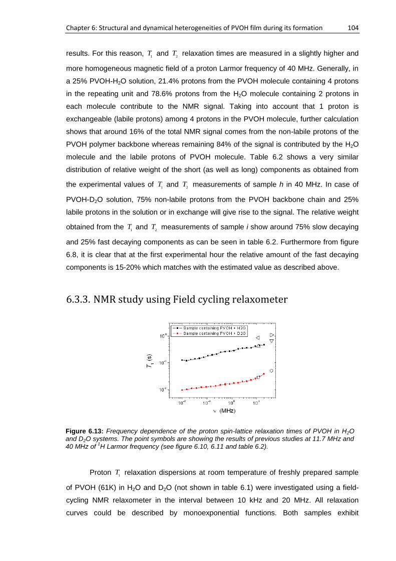
Chapter 6: Structural and dynamical heterogeneities of PVOH film during its formation 104
results. For this reason, 1
T and 2
T relaxation times are measured in a slightly higher and
more homogeneous magnetic field of a proton Larmor frequency of 40 MHz. Generally, in
a 25% PVOH-H2O solution, 21.4% protons from the PVOH molecule containing 4 protons
in the repeating unit and 78.6% protons from the H2O molecule containing 2 protons in
each molecule contribute to the NMR signal. Taking into account that 1 proton is
exchangeable (labile protons) among 4 protons in the PVOH molecule, further calculation
shows that around 16% of the total NMR signal comes from the non-labile protons of the
PVOH polymer backbone whereas remaining 84% of the signal is contributed by the H2O
molecule and the labile protons of PVOH molecule. Table 6.2 shows a very similar
distribution of relative weight of the short (as well as long) components as obtained from
the experimental values of 1
T and 2
T measurements of sample h in 40 MHz. In case of
PVOH-D2O solution, 75% non-labile protons from the PVOH backbone chain and 25%
labile protons in the solution or in exchange will give rise to the signal. The relative weight
obtained from the 1
T and 2
T measurements of sample i show around 75% slow decaying
and 25% fast decaying components as can be seen in table 6.2. Furthermore from figure
6.8, it is clear that at the first experimental hour the relative amount of the fast decaying
components is 15-20% which matches with the estimated value as described above.
6.3.3. NMR study using Field cycling relaxometer
Proton 1
T relaxation dispersions at room temperature of freshly prepared sample
of PVOH (61K) in H2O and D2O (not shown in table 6.1) were investigated using a field-
cycling NMR relaxometer in the interval between 10 kHz and 20 MHz. All relaxation
curves could be described by monoexponential functions. Both samples exhibit
Figure 6.13: Frequency dependence of the proton spin-lattice relaxation times of PVOH in H2O and D2O systems. The point symbols are showing the results of previous studies at 11.7 MHz and 40 MHz of
1H Larmor frequency (see figure 6.10, 6.11 and table 6.2).
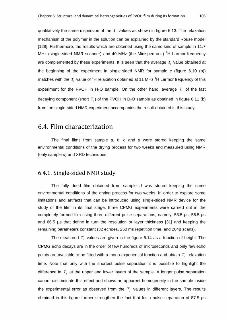
Chapter 6: Structural and dynamical heterogeneities of PVOH film during its formation 105
qualitatively the same dispersion of the 1
T values as shown in figure 6.13. The relaxation
mechanism of the polymer in the solution can be explained by the standard Rouse model
[128]. Furthermore, the results which are obtained using the same kind of sample in 11.7
MHz (single-sided NMR scanner) and 40 MHz (the Minispec unit) 1H Larmor frequency
are complemented by these experiments. It is seen that the average 1
T value obtained at
the beginning of the experiment in single-sided NMR for sample c (figure 6.10 (b))
matches with the 1
T value of 1H relaxation obtained at 11 MHz 1H Larmor frequency of this
experiment for the PVOH in H2O sample. On the other hand, average 1
T of the fast
decaying component (short 1
T ) of the PVOH in D2O sample as obtained in figure 6.11 (b)
from the single-sided NMR experiment accompanies the result obtained in this study.
6.4. Film characterization
The final films from sample a, b, c and d were stored keeping the same
environmental conditions of the drying process for two weeks and measured using NMR
(only sample d) and XRD techniques.
6.4.1. Single-sided NMR study
The fully dried film obtained from sample d was stored keeping the same
environmental conditions of the drying process for two weeks. In order to explore some
limitations and artifacts that can be introduced using single-sided NMR device for the
study of the film in its final stage, three CPMG experiments were carried out in the
completely formed film using three different pulse separations, namely, 53.5 µs, 56.5 µs
and 66.5 µs that define in turn the resolution or layer thickness [31] and keeping the
remaining parameters constant (32 echoes, 250 ms repetition time, and 2048 scans).
The measured 2
T values are given in the figure 6.14 as a function of height. The
CPMG echo decays are in the order of few hundreds of microseconds and only few echo
points are available to be fitted with a mono-exponential function and obtain 2
T relaxation
time. Note that only with the shortest pulse separation it is possible to highlight the
difference in 2
T at the upper and lower layers of the sample. A longer pulse separation
cannot discriminate this effect and shows an apparent homogeneity in the sample inside
the experimental error as observed from the 2
T values in different layers. The results
obtained in this figure further strengthen the fact that for a pulse separation of 87.5 µs
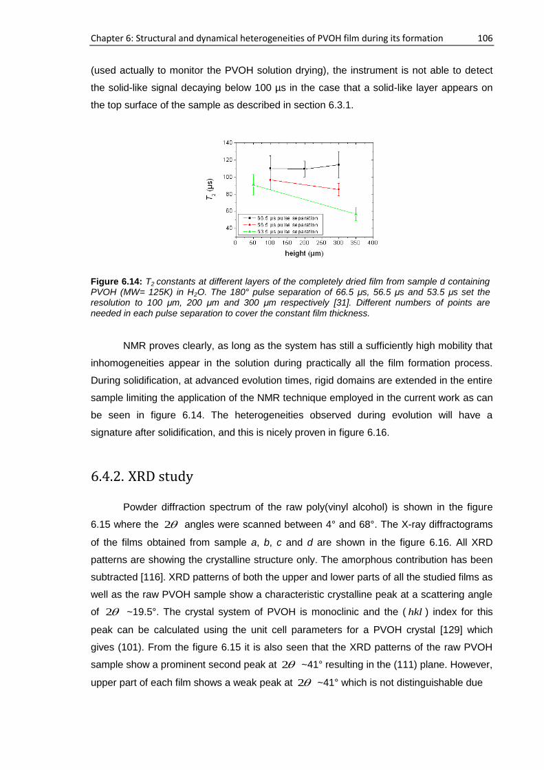
Chapter 6: Structural and dynamical heterogeneities of PVOH film during its formation 106
(used actually to monitor the PVOH solution drying), the instrument is not able to detect
the solid-like signal decaying below 100 µs in the case that a solid-like layer appears on
the top surface of the sample as described in section 6.3.1.
NMR proves clearly, as long as the system has still a sufficiently high mobility that
inhomogeneities appear in the solution during practically all the film formation process.
During solidification, at advanced evolution times, rigid domains are extended in the entire
sample limiting the application of the NMR technique employed in the current work as can
be seen in figure 6.14. The heterogeneities observed during evolution will have a
signature after solidification, and this is nicely proven in figure 6.16.
6.4.2. XRD study
Powder diffraction spectrum of the raw poly(vinyl alcohol) is shown in the figure
6.15 where the 2 angles were scanned between 4° and 68°. The X-ray diffractograms
of the films obtained from sample a, b, c and d are shown in the figure 6.16. All XRD
patterns are showing the crystalline structure only. The amorphous contribution has been
subtracted [116]. XRD patterns of both the upper and lower parts of all the studied films as
well as the raw PVOH sample show a characteristic crystalline peak at a scattering angle
of 2 ~19.5°. The crystal system of PVOH is monoclinic and the ( hkl ) index for this
peak can be calculated using the unit cell parameters for a PVOH crystal [129] which
gives (101). From the figure 6.15 it is also seen that the XRD patterns of the raw PVOH
sample show a prominent second peak at 2 ~41° resulting in the (111) plane. However,
upper part of each film shows a weak peak at 2 ~41° which is not distinguishable due
Figure 6.14: T2 constants at different layers of the completely dried film from sample d containing PVOH (MW= 125K) in H2O. The 180° pulse separation of 66.5 μs, 56.5 μs and 53.5 μs set the resolution to 100 μm, 200 μm and 300 μm respectively [31]. Different numbers of points are needed in each pulse separation to cover the constant film thickness.
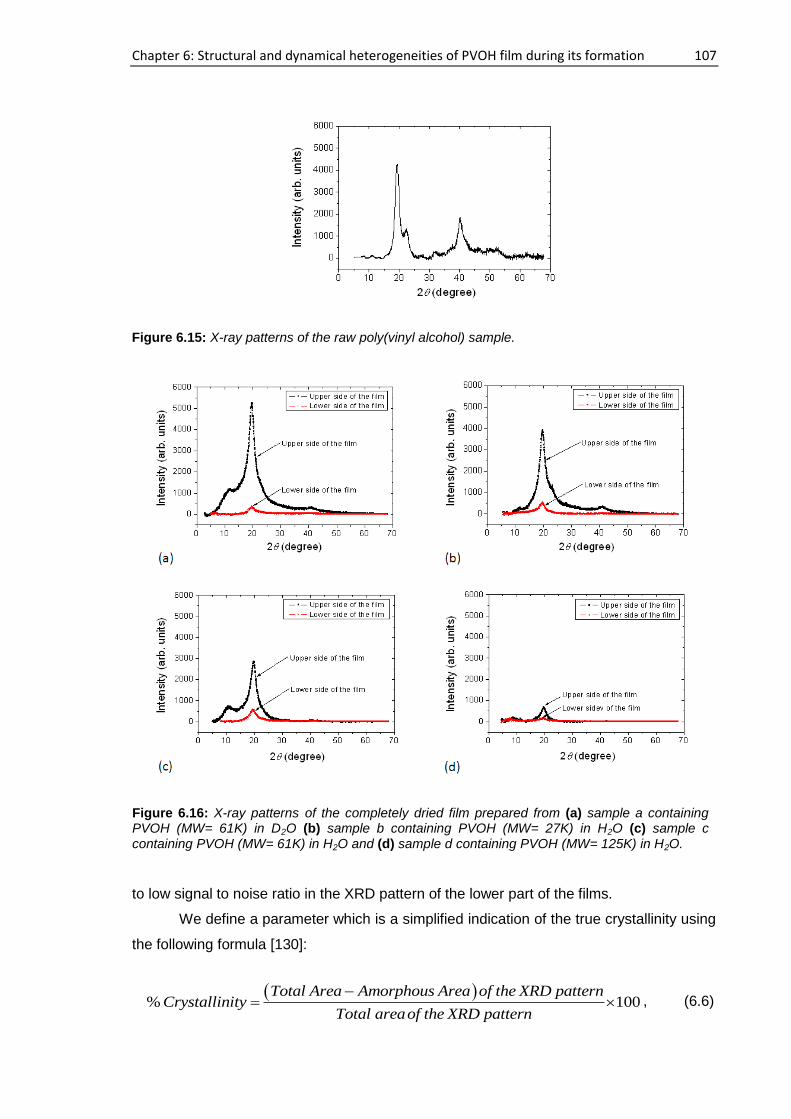
Chapter 6: Structural and dynamical heterogeneities of PVOH film during its formation 107
to low signal to noise ratio in the XRD pattern of the lower part of the films.
We define a parameter which is a simplified indication of the true crystallinity using
the following formula [130]:
% 100Total Area Amorphous Area of the XRD pattern
CrystallinityTotal areaof the XRD pattern
, (6.6)
Figure 6.15: X-ray patterns of the raw poly(vinyl alcohol) sample.
Figure 6.16: X-ray patterns of the completely dried film prepared from (a) sample a containing PVOH (MW= 61K) in D2O (b) sample b containing PVOH (MW= 27K) in H2O (c) sample c containing PVOH (MW= 61K) in H2O and (d) sample d containing PVOH (MW= 125K) in H2O.
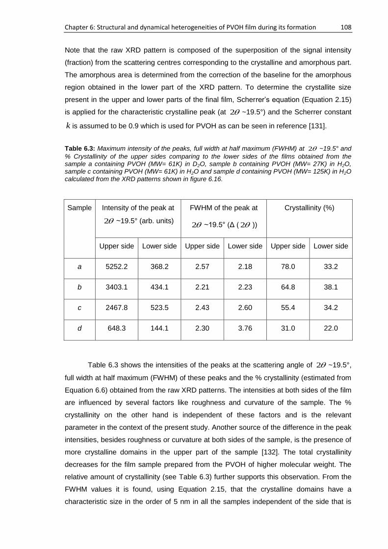
Chapter 6: Structural and dynamical heterogeneities of PVOH film during its formation 108
Note that the raw XRD pattern is composed of the superposition of the signal intensity
(fraction) from the scattering centres corresponding to the crystalline and amorphous part.
The amorphous area is determined from the correction of the baseline for the amorphous
region obtained in the lower part of the XRD pattern. To determine the crystallite size
present in the upper and lower parts of the final film, Scherrer‟s equation (Equation 2.15)
is applied for the characteristic crystalline peak (at 2 ~19.5°) and the Scherrer constant
k is assumed to be 0.9 which is used for PVOH as can be seen in reference [131].
Table 6.3: Maximum intensity of the peaks, full width at half maximum (FWHM) at 2 ~19.5° and
% Crystallinity of the upper sides comparing to the lower sides of the films obtained from the sample a containing PVOH (MW= 61K) in D2O, sample b containing PVOH (MW= 27K) in H2O, sample c containing PVOH (MW= 61K) in H2O and sample d containing PVOH (MW= 125K) in H2O calculated from the XRD patterns shown in figure 6.16.
Sample Intensity of the peak at
2 ~19.5° (arb. units)
FWHM of the peak at
2 ~19.5° (Δ ( 2 ))
Crystallinity (%)
Upper side Lower side Upper side Lower side Upper side Lower side
a 5252.2 368.2 2.57 2.18 78.0 33.2
b 3403.1 434.1 2.21 2.23 64.8 38.1
c 2467.8 523.5 2.43 2.60 55.4 34.2
d 648.3 144.1 2.30 3.76 31.0 22.0
Table 6.3 shows the intensities of the peaks at the scattering angle of 2 ~19.5°,
full width at half maximum (FWHM) of these peaks and the % crystallinity (estimated from
Equation 6.6) obtained from the raw XRD patterns. The intensities at both sides of the film
are influenced by several factors like roughness and curvature of the sample. The %
crystallinity on the other hand is independent of these factors and is the relevant
parameter in the context of the present study. Another source of the difference in the peak
intensities, besides roughness or curvature at both sides of the sample, is the presence of
more crystalline domains in the upper part of the sample [132]. The total crystallinity
decreases for the film sample prepared from the PVOH of higher molecular weight. The
relative amount of crystallinity (see Table 6.3) further supports this observation. From the
FWHM values it is found, using Equation 2.15, that the crystalline domains have a
characteristic size in the order of 5 nm in all the samples independent of the side that is
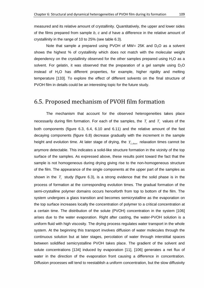
Chapter 6: Structural and dynamical heterogeneities of PVOH film during its formation 109
measured and its relative amount of crystallinity. Quantitatively, the upper and lower sides
of the films prepared from sample b, c and d have a difference in the relative amount of
crystallinity in the range of 10 to 25% (see table 6.3).
Note that sample a prepared using PVOH of MW= 25K and D2O as a solvent
shows the highest % of crystallinity which does not match with the molecular weight
dependency on the crystallinity observed for the other samples prepared using H2O as a
solvent. For gelatin, it was observed that the preparation of a gel sample using D2O
instead of H2O has different properties, for example, higher rigidity and melting
temperature [133]. To explore the effect of different solvents on the final structure of
PVOH film in details could be an interesting topic for the future study.
6.5. Proposed mechanism of PVOH film formation
The mechanism that account for the observed heterogeneities takes place
necessarily during film formation. For each of the samples, the 1
T and 2
T values of the
both components (figure 6.3, 6.4, 6.10 and 6.11) and the relative amount of the fast
decaying components (figure 6.8) decrease gradually with the increment in the sample
height and evolution time. At later stage of drying, the 2,shortT relaxation times cannot be
anymore detectable. This indicates a solid-like structure formation in the vicinity of the top
surface of the samples. As expressed above, these results point toward the fact that the
sample is not homogeneous during drying giving rise to the non-homogeneous structure
of the film. The appearance of the single components at the upper part of the samples as
shown in the 2
T study (figure 6.3), is a strong evidence that the solid phase is in the
process of formation at the corresponding evolution times. The gradual formation of the
semi-crystalline polymer domains occurs henceforth from top to bottom of the film. The
system undergoes a glass transition and becomes semicrystalline as the evaporation on
the top surface increases locally the concentration of polymer to a critical concentration at
a certain time. The distribution of the solute (PVOH) concentration in the system [106]
arises due to the water evaporation. Right after casting, the water-PVOH solution is a
uniform fluid with high viscosity. The drying process regulates water transport in the whole
system. At the beginning this transport involves diffusion of water molecules through the
continuous solution but at later stages, percolation of water through interstitial spaces
between solidified semicrystalline PVOH takes place. The gradient of the solvent and
solute concentrations [134] induced by evaporation [11], [106] generates a net flux of
water in the direction of the evaporation front causing a difference in concentration.
Diffusion processes will tend to reestablish a uniform concentration, but the slow diffusivity
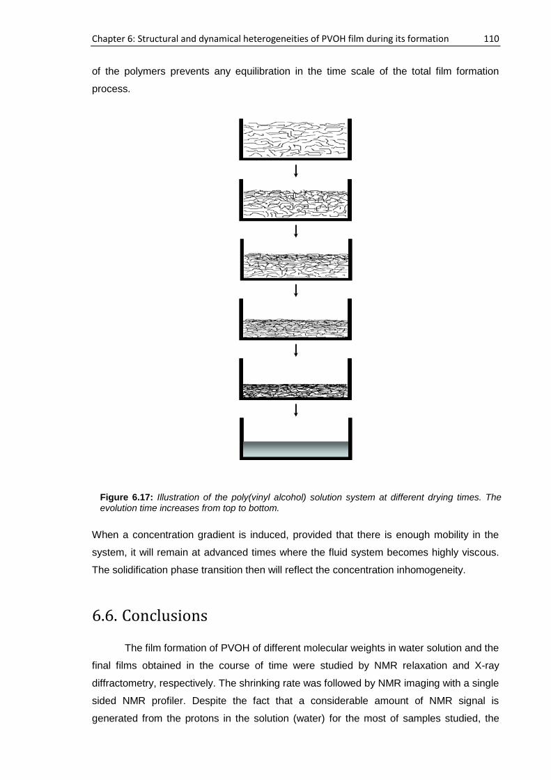
Chapter 6: Structural and dynamical heterogeneities of PVOH film during its formation 110
of the polymers prevents any equilibration in the time scale of the total film formation
process.
When a concentration gradient is induced, provided that there is enough mobility in the
system, it will remain at advanced times where the fluid system becomes highly viscous.
The solidification phase transition then will reflect the concentration inhomogeneity.
6.6. Conclusions
The film formation of PVOH of different molecular weights in water solution and the
final films obtained in the course of time were studied by NMR relaxation and X-ray
diffractometry, respectively. The shrinking rate was followed by NMR imaging with a single
sided NMR profiler. Despite the fact that a considerable amount of NMR signal is
generated from the protons in the solution (water) for the most of samples studied, the
Figure 6.17: Illustration of the poly(vinyl alcohol) solution system at different drying times. The evolution time increases from top to bottom.
Chapter 6: Structural and dynamical heterogeneities of PVOH film during its formation 111
results are in a complete agreement with the case where D2O is used as a solution
instead. As mentioned above, the detection of a “skin-layer” using this single-sided
scanner is difficult. However, the remarkable fact in this work by NMR is the evidence of a
gradual slowing down of the molecular dynamics in the direction of the evaporating
surface. This is indicated by the two experimental parameters 1
T and 2
T .
By the determination of the relaxation parameters 1T and
2T it could be traced out
that the effect of the evaporation of the solvent molecules in the dynamics of the solution
induces a dynamic heterogeneity of the polymer molecules across the film thickness for all
the molecular weights. The local evaporation process taking place at the air-sample
interface further influences the migration of polymer chains, inducing differences in
concentration along the whole system. The direct consequence is the reduction in the
mobility of the polymer chains towards the surface where evaporation takes place. These
spatial heterogeneities influence the local dynamical behavior of the system and the
profile of relaxation times becomes progressively asymmetric during the evolution time.
The shorter relaxation times on the top surface at later stages of film formation indicate
the presence of more immobile polymer chains. Once the system has completely solidified
below certain water content, the measured 2T relaxation times reflect the dynamics of the
amorphous part (as expressed above, the single sided scanner is not sensitive to solid
NMR signals). This reveals that the amorphous domain has different dynamics along the
film. Taking into account that more crystallization domains are found on top of the film
from the XRD study, together with the fact that the polymer system is well below the glass
transition temperature, the dynamics of the amorphous part is restricted by the presence
of the crystalline domains in the sense of confinement i.e., there is a geometrical
confinement. The effect of the molecular weight on the structure of the films is the
formation of more crystalline phase at the top surface in the case that PVOH has the
lowest molecular weight. This can be seen in table 6.3, where the ratio of crystallinity
between the upper and the lower parts decreases with the increase in molecular weight.
In conclusion, an evidence of heterogeneous dynamical restriction of the
amorphous part of the final film by the presence of more crystalline domains is found in
the final film along the vertical direction, induced during its formation process and
influenced by the molecular weight of the polymer.
112
Chapter 7
Summary and outlook
If I’d had some set idea of a finish line,
don’t you think I would have crossed it years ago?
Bill Gates
During the last few decades, increasing efforts have been paid to the investigation
of the biopolymer films for new applications. However, the biopolymer film formation
process is still not fully understood, and requires considerable attention. The goal of this
thesis has been the study of the film formation of environmentally friendly polymers and
their characterization. Two biopolymers, gelatin (from animal origin) and starch (from plant
origin), were chosen because of their abundance as well as diversify and promising field
of applications. Poly(vinyl alcohol) (PVOH), an environmentally friendly synthetic polymer,
having a simple structure compared to gelatin and starch, was studied as well. For each
polymer sample, a set of systematic experiments were designed to follow the drying
process using low-field single-sided nuclear magnetic resonance (NMR) device.
The remarkable aspect in these experiments is the discrimination of the dynamics
among different layers of microscopic resolution that is possible with the technique using
single-sided NMR scanner. Time-dependent NMR profiles were measured at different
layers of the sample using this scanner. Longitudinal (1T ) and transverse (
2T ) relaxation
times, which prove directly the dynamics of the system [32], were obtained from the echo-
decay for each profile point. X-ray diffraction (XRD) and differential scanning calorimetry
(DSC) techniques along with the NMR technique were used to characterize the dried
films. The employed methods represent a suitable measure for indicating the residual
mobility of the system.
Chapter 7: Summary and outlook 113
The investigations of the film formation and their characterization on these polymer
systems are listed and summarized as below:
Gelatin solutions were prepared varying the initial concentrations of gelatin (1%,
2% and 10%) in H2O or D2O (w/v) followed by casting. Film formation was
investigated in situ during evaporation of the solvent. It was found that when the
gelatin film is approaching the final drying stage, the 2T values of the sample near
the substrate decreases more compared with the value at the vicinity of the air-
sample interface. This spatial heterogeneity is also observed in the 1T values at a
comparatively low 1H Larmor frequency of 11.7 MHz, being sensitive for a
reduction in overall molecular mobility. XRD study confirmed that the heterogeneity
observed during the film formation persists in the final film [SG 1], [SG 2].
A solution using 10% gelatin in H2O (w/v) was prepared. Same amount of sample
was cast in a series of Petri dishes and left to evolve under identical conditions.
Each sample was subjected to study using high-field NMR and DSC while the film
was forming. Development of collagen-like triple helix structure (renaturation) was
observed in the course of gelatin film formation as revealed by these studies. It
was found that the renaturation process takes place for a short period comparing
to the total time of film formation [SG 3].
Gelatin films were prepared from the solutions of different initial concentrations
(1% to 30%) in H2O (w/v). The films were calibrated at four different relative
humidity (20%, 43%, 75% and 90%) conditions. The influence of initial
concentration and humidity on the dried gelatin film was investigated. It was found
that there is an apparent effect of humidity on the relaxation and thermal properties
of the gelatin film which is less pronounced in case of initial concentration [SG 4].
Film formation process from an aqueous sample of 1% and 5% corn starch (w/v)
was successfully studied for the first time using micro camera and single-sided
NMR scanner. The dried film was characterized using NMR and XRD techniques.
It was found that the molecular mobility of these two samples varied notably at
different stages of film formation. At an intermediate stage, a gradual decrease in
mobility of 1% starch containing sample towards the air-sample interface was
observed although 5% starch containing sample was homogeneous all along the
sample height. At a later stage, heterogeneity in the dynamics was observed in
both samples showing that the bottom part of the sample is less mobile than the
upper part. This effect was more evident in the 5% starch containing sample and
Chapter 7: Summary and outlook 114
the XRD study confirmed that the structural heterogeneity persists in the final film
obtained from this sample [SG 5].
The film formation out of a concentrated aqueous solution of poly(vinyl alcohol)
(PVOH) of different molecular weights subject to solvent evaporation was
investigated by means of NMR methods and by XRD of the final, solid film. A
dynamic heterogeneity of the polymer molecules across the film thickness was
observed after a certain time. This behavior approximately corresponds to a
change in evaporation rate, indicated by a pronounced decrease of the film
shrinking rate. This work confirms that a pronounced reduction in mobility of the
polymer chains is observed towards the air-sample interface; however, the
variation remains gradual for the whole accessible drying period and a transition
towards a well-defined solid skin is not observed from the NMR relaxation data.
Subsequent analysis of the completely dried film by X-ray diffractometry, however,
reveals that the crystallinity at the top surface is indeed considerably higher than
that at the bottom [SG 6], [SG 7].
The above presented studies open the door to several possibilities for future
research. It will be necessary to study the influence of the precipitation of the biopolymer
chains on the film formation. It was observed that the profile edges near to the air-sample
interface vary with concentrations of the sample which was not fully understood along this
work. To explore this occurrence would be a promising approach. Although we have
extensively studied the structural heterogeneity of the final dried film obtained from
gelatin, starch and PVOH samples using low-field NMR and XRD methods, still there are
scopes to explore. For instance, extraction of the thin layers from the upper and lower
surfaces of a dried film could be helpful for further characterization of the film and to
obtain quantitative information regarding the heterogeneity using solid-state NMR or other
techniques. Based on the results obtained in this thesis, preparation and characterization
of the multilayer biopolymer film could be a potential approach in future.
Publications by the Author as a part of this work 115
Publications by the Author as a part of this work
[SG 1]. S. Ghoshal, C. Mattea and S. Stapf. Inhomogeneity in the drying process of
gelatin film formation: NMR microscopy and relaxation study. Chemical Physics
Letters, 485, 343-347, 2010.
[SG 2]. S. Ghoshal, C. Mattea, P. Denner and S. Stapf. Heterogeneities in gelatin film
formation using single-sided NMR. Journal of Physical Chemistry B, 114,
16356-16363, 2010. [Won the best paper award of TU Ilmenau 2010]
[SG 3]. S. Ghoshal, C. Mattea and S. Stapf. Gelatin film formation studied by high-field
NMR and DSC techniques. (In preparation)
[SG 4]. S. Ghoshal, C. Mattea and S. Stapf. Concentration and humidity effects on
gelatin films studied by NMR. (In preparation)
[SG 5]. S. Ghoshal, C. Mattea, P. Denner and S. Stapf. Drying of starch biopolymer:
NMR microscopy study. (In preparation)
[SG 6]. S. Ghoshal, P. Denner, S. Stapf and C. Mattea. Structural and dynamical
heterogeneities in PVA films induced by evaporation during the formation
process. Chemical Physics Letters, 515, 231-234, 2011.
[SG 7]. S. Ghoshal, P. Denner, S. Stapf and C. Mattea. Study of film formation of
Poly(vinyl alcohol). Macromolecules, 45, 1913-1923, 2012.
Bibliography 116
Bibliography
[1] F. W. Billmeyer. Textbook of polymer science. John Wiley & Sons: New York, 1984.
[2] D. Feldman and A. Barbalata. Synthetic Polymers: technology, properties,
applications. Chapman & Hall: London, UK, 1996.
[3] G. Griffin. Chemistry and Technology of Biodegradable Polymers. Springer, 1993.
[4] A. Gennadios. Protein-based films and coatings. CRC Press: Boca Raton, 2002.
[5] M. A. García, M. N. Martino and N. E. Zaritzky. Microstructural characterization of
plasticized starch-based films. Starch - Stärke, 52 (4), 118-124, 2000.
[6] C. S. S. R. Kumar. Nanostructured thin films and surfaces. Wiley-VCH: Weinheim,
2010.
[7] I. Yakimets, S. S. Paes, N. Wellner, A. C. Smith, R. H. Wilson and J. R. Mitchell.
Effect of water content on the structural reorganization and elastic properties of
biopolymer films: a comparative study. Biomacromolecules, 8 (5), 1710–1722,
2007.
[8] E. Kristo, C. Biliaderis and A. Zampraka. Water vapour barrier and tensile
properties of composite caseinate-pullulan films: Biopolymer composition effects
and impact of beeswax lamination. Food Chemistry, 101 (2), 753–764, 2007.
[9] D. Thirathumthavorn and S. Charoenrein. Aging effects on sorbitol- and non-
crystallizing sorbitol-plasticized tapioca starch films. Starch - Stärke, 59 (10), 493–
497, 2007.
[10] J. F. Martucci and R. A. Ruseckaite. Tensile properties, barrier properties, and
biodegradation in soil of compression-Molded gelatin-dialdehyde starch films.
Journal of Applied Polymer Science, 112 (4), 2166–2178, 2009.
[11] S.-S. Wong, S. A. Altinkaya and S. K. Mallapragada. Understanding the effect of
skin formation on the removal of solvents from semicrystalline polymers. Journal of
Polymer Science Part B: Polymer Physics, 43 (22), 3191–3204, 2005.
Bibliography 117
[12] J. C. H. Hwa. Mechanism of film formation from latices. Phenomenon of
flocculation. Journal of Polymer Science Part A: General Papers, 2 (2), 785–796,
1964.
[13] S. Erich, H. Huinink, O. Adan, J. Laven and A. Esteves. The influence of the
pigment volume concentration on the curing of alkyd coatings: a 1D MRI depth
profiling study. Progress in Organic Coatings, 63 (4), 399–404, 2008.
[14] A. F. Routh and W. B. Russel. A process model for latex film formation: limiting
regimes for individual driving forces. Langmuir, 15 (22), 7762–7773, 1999.
[15] A. Veis. The macromolecular chemistry of gelatin. Academic Press: New York,
London, 1964.
[16] J. N. BeMiller and R. L. Whistler. Starch: chemistry and technology. Academic
Press, 2009.
[17] V. Goodship and D. Jacobs. Polyvinyl alcohol: materials, processing and
applications. Smithers Rapra Technology: Shrewsbury, 2005.
[18] M. O. Ngui and S. K. Mallapragada. Understanding isothermal semicrystalline
polymer drying: mathematical models and experimental characterization. Journal of
Polymer Science Part B: Polymer Physics, 36 (15), 2771–2780, 1998.
[19] M. O. Ngui and S. K. Mallapragada. Mechanistic investigation of drying regimes
during solvent removal from poly(vinyl alcohol) films. Journal of Applied Polymer
Science, 72, 1913–1920, 1999.
[20] M. O. Ngui and S. K. Mallapragada. Quantitative analysis of crystallization and skin
formation during isothermal solvent removal from semicrystalline polymers. Polymer,
40 (19), 5393–5400, 1999.
[21] S.-S. Wong, S. A. Altinkaya and S. K. Mallapragada. Drying of semicrystalline
polymers: mathematical modeling and experimental characterization of poly(vinyl
alcohol) films. Polymer, 45, 5151–5161, 2004.
[22] E. Ciampi and P. J. McDonald. Skin formation and water distribution in
semicrystalline polymer layers cast from solution: a magnetic resonance imaging
study. Macromolecules, 36 (22), 8398–8405, 2003.
Bibliography 118
[23] Y.-T. Kim, Y.-S. Hong, R. M. Kimmel, J.-H. Rho and C.-H. Lee. New approach for
characterization of gelatin biopolymer films using proton behavior determined by low
field 1H NMR spectrometry. Journal of Agricultural and Food Chemistry, 55 (26),
10678–10684, 2007.
[24] A. Traoré, L. Foucat and J. P. Renou. 1H NMR studies: dynamics of water in gelatin.
European Biophysics Journal, 29 (3), 159–164, 2000.
[25] M.-C. Vackier, B. P. Hills and D. N. Rutledge. An NMR relaxation study of the state
of water in gelatin gels. Journal of Magnetic Resonance, 138 (1), 36–42, 1999.
[26] A. E. Aliev. Solid-state NMR studies of collagen-based parchments and gelatin.
Biopolymers, 77 (4), 230–245, 2005.
[27] V. Svoboda and B. Y. Liaw. In situ transient study of polymer film growth via
simultaneous correlation of charge, mass, and ellipsometric measurements. Pure
and Applied Chemistry, 80 (11), 2439–2449, 2008.
[28] M. Peura, T. Karppinen, A. Soovre, A. Salmi, M. Tenkanen, E. Hæggström and R.
Serimaa. Crystallization and shear modulus of a forming biopolymer film determined
by in situ x-ray diffraction and ultrasound reflection methods. Journal of Applied
Physics, 104 (2), 23513, 2008.
[29] Y. Wang, D. Juhué, M. A. Winnik, O. Leung and M. C. Goh. Atomic force
microscopy study of latex film formation. Langmuir, 8, 760–762, 1992.
[30] A. Fissel, J. Dabrowski and H. J. Osten. Photoemission and ab initio theoretical
study of interface and film formation during epitaxial growth and annealing of
praseodymium oxide on Si(001). Journal of Applied Physics, 91, 8986–8991, 2002.
[31] F. Casanova, J. Perlo and B. Blümich. Single-sided NMR. Springer, 2011.
[32] A. Abragam. The principles of nuclear magnetism. Clarendon Press, Oxford
University Press: Oxford, New York, 1961.
[33] P. T. Callaghan. Principles of nuclear magnetic resonance microscopy. Clarendon
Press, Oxford University Press: Oxford, New York, 1991.
Bibliography 119
[34] F. A. Bovey, L. Jelinski and P. A. Mirau. Nuclear magnetic resonance spectroscopy.
Academic Press: San Diego, 1988.
[35] M. H. Levitt. Spin dynamics: basics of nuclear magnetic resonance. John Wiley &
Sons, 2008.
[36] H. Friebolin. Basic one- and two-dimensional NMR spectroscopy. Wiley-VCH:
Weinheim, 2005.
[37] R. Macomber. A complete introduction to modern NMR spectroscopy. Wiley, 1998.
[38] D. Cullity and S. R. Stock. Elements of X-ray diffraction. Prentice Hall: Upper Saddle
River, NJ, 2001.
[39] C. Suryanarayana and M. G. Norton. X-Ray diffraction. Plenum Press: New York,
1998.
[40] P. Gabbott. Principles and applications of thermal analysis. Blackwell Pub.: Oxford,
Ames, Iowa, 2008.
[41] J. D. Menczel and R. B. Prime. Thermal analysis of polymers. John Wiley: Hoboken,
NJ, 2009.
[42] G. Höhne, W. Hemminger and H.-J. Flammersheim. Differential scanning
calorimetry. Springer: Berlin, New York, 2003.
[43] R. W. Biederman, M. Doyle, R. W. W. Biederman and J. Yamrozik. The
cardiovascular MRI tutorial: lectures and learning. Lippincott Williams & Wilkins,
2007.
[44] R. Kimmich. NMR: tomography, diffusometry, relaxometry. Springer, 1997.
[45] G. N. Ramachandran and C. Ramakrishnan. Biochemistry of collagen. Plenum
Press: New York, 1976.
[46] J. Bella, B. Brodsky and H. M. Berman. Hydration structure of a collagen peptide.
Structure, 3, 893–906, 1995.
Bibliography 120
[47] F. Gul-E-Noor, M. A. Khan, S. Ghoshal, R. Mazid, A. M. S. Chowdhury and R. A.
Khan. Grafting of 2-ethylhexyl acrylate with urea on to gelatin film by gamma
radiation. Journal of Macromolecular Science, Part A, 46 (6), 615–624, 2009.
[48] S.-S. Choi and J. Regenstein. Physicochemical and sensory characteristics of fish
gelatin. Journal of Food Science, 65, 194–199, 2000.
[49] P. J. A. Sobral, F. C. Menegalli, M. D. Hubinger and M. A. Roques. Mechanical,
water vapor barrier and thermal properties of gelatin based edible films. Food
Hydrocolloids, 15 (4-6), 423–432, 2001.
[50] P. C. Griffith, P. Stilbs, A. M. Howe and T. Cosgrove. A Self-Diffusion Study of the
complex formed by sodium dodecyl sulfate and gelatin in aqueous solutions.
Langmuir, 12 (12), 2884–2893, 1996.
[51] M. N. Belgacem and A. Gandini. Monomers, polymers and composites from
renewable resources. Elsevier: Amsterdam, London, 2008.
[52] R. Talja. Preparation and characterization of potato starch films plasticized with
polyols. PhD Thesis, Department of Food Technology, University of Helsinki, 2007.
[53] T. Barsby, A. Donald, P. Frazier and Royal Society of Chemistry (Great Britain)
Food Chemistry Group. Starch: advances in structure and function. Royal Society of
Chemistry, 2001.
[54] P. J. Jenkins and A. M. Donald. The influence of amylose on starch granule
structure. International Journal of Biological Macromolecules, 17 (6), 315–321,
1995.
[55] S. Jobling. Improving starch for food and industrial applications. Current Opinion in
Plant Biology, 7 (2), 210–218, 2004.
[56] K. Krogars, O. Antikainen, J. Heinämäki, N. Laitinen and J. Yliruusi. Tablet film-
coating with amylose-rich maize starch. European Journal of Pharmaceutical
Science, 17, 23–30, 2002.
[57] A. Jansson and F. Thuvander. Influence of thickness on the mechanical properties
for starch films. Carbohydrate Polymers, 56 (4), 499–503, 2004.
Bibliography 121
[58] R. A. Talja, H. Helén, Y. H. Roos and K. Jouppila. Effect of various polyols and
polyol contents on physical and mechanical properties of potato starch-based films.
Carbohydrate Polymers, 67 (3), 288–295, 2007.
[59] Y. Zhang and J. H. Han. Mechanical and thermal characteristics of pea starch films
plasticized with monosaccharides and polyols. Journal of Food Science, 71 (2), E
109–118, 2006.
[60] A. Steinbüchel and S. Matsumura. Miscellaneous biopolymers and biodegradation
of synthetic polymers. Wiley-VCH: Weinheim, Cambridge, 2003.
[61] N. Hodgkinson and M. Taylor. Thermoplastic poly (Vinyl Alcohol) (PVOH). Materials
World, 8, 24–25, 2000.
[62] L. E. Stephans and N. Foster. Magnetization-transfer NMR analysis of aqueous
poly(vinyl alcohol) gels: effect of hydrolysis and storage temperature on network
formation. Macromolecules, 31 (5), 1644–1651, 1998.
[63] M. Shibayama, H. Kurokawa, S. Nomura, S. Roy, R. S. Stein and W. L. Wu. Small-
angle neutron scattering studies on chain asymmetry of coextruded poly(vinyl
alcohol) film. Macromolecules, 23 (5), 1438–1443, 1990.
[64] C. A. Finch. Polyvinyl alcohol: developments. Wiley: Chichester, New York, 1992.
[65] J. L. Valentin, D. Lopez, R. Hernandez, C. Mijangos and K. Saalwaächter. Structure
of poly(vinyl alcohol) cryo-hydrogels as studied by proton low-field NMR
spectroscopy. Macromolecules, 42 (1), 263–272, 2009.
[66] J. B. Chang, J. H. Hwang, J. S. Park and J. P. Kim. The effect of dye structure on
the dyeing and optical properties of dichroic dyes for PVA polarizing film. Dyes and
Pigments, 88 (3), 366–371, 2011.
[67] C.-C. Yang and Y.-J. Lee. Preparation of the acidic PVA/MMT nanocomposite
polymer membrane for the direct methanol fuel cell (DMFC). Thin Solid Films, 517
(17), 4735–4740, 2009.
[68] K. Krogars, J. Heinämäki, M. Karjalainen, J. Rantanen, P. Luukkonen and J.
Yliruusi. Development and characterization of aqueous amylose-rich maize starch
Bibliography 122
dispersion for film formation. European Journal of Pharmaceutics and
Biopharmaceutics, 56 (2), 215–221, 2003.
[69] B. Blümich, J. Perlo and F. Casanova. Mobile single-sided NMR. Progress in
Nuclear Magnetic Resonance Spectroscopy, 52 (4), 197–269, 2008.
[70] J. Perlo, F. Casanova and B. Blümich. Profiles with microscopic resolution by single-
sided NMR. Journal of Magnetic Resonance, 176 (1), 64–70, 2005.
[71] S. Meiboom and D. Gill. Modified Spin-echo method for measuring nuclear
relaxation times. Review of Scientific Instruments, 29 (8), 688–691, 1958.
[72] O. Neudert. Implementation, optimization and application of unconventional diffusion
measurement techniques for single-sided NMR. Masterarbeit, Technische Physik,
Technische Universität Ilmenau, 2010.
[73] S. Stapf and S. Han. NMR imaging in chemical engineering. Wiley-VCH, 2006.
[74] N. Bloembergen. Nuclear magnetic resonance. W. A. Benjamin: New York, 1961.
[75] E. L. Hahn. Spin echoes. Physical Review, 80 (4), 580–594, 1950.
[76] K. Saalwächter, M. Gottlieb, R. Liu and W. Oppermann. Gelation as studied by
proton multiple-quantum NMR. Macromolecules, 40 (5), 1555–1561, 2007.
[77] H. Y. Carr and E. M. Purcell. Effects of diffusion on free precession in nuclear
magnetic resonance experiments. Physical Review, 94 (3), 630–638, 1954.
[78] R. L. Vold, J. S. Waugh, M. P. Klein and D. E. Phelps. Measurement of spin
relaxation in complex systems. The Journal of Chemical Physics, 48 (8), 3831,
1968.
[79] R. Kimmich and E. Anoardo. Field-cycling NMR relaxometry. Progress in Nuclear
Magnetic Resonance Spectroscopy, 44 (3-4), 257–320, 2004.
[80] J. L. Gornall and E. M. Terentjev. Concentration-temperature superposition of helix
folding rates in gelatin. Physical Review Letters, 99 (2), 028304-4, 2007.
[81] A. Bigi, S. Panzavolta and K. Rubini. Relationship between triple-helix content and
mechanical properties of gelatin films. Biomaterials, 25 (25), 5675–5680, 2004.
Bibliography 123
[82] L. Friedman and E. O. Kraemer. The structure of gelatin gels from studies of
diffusion. Journal of the American Chemical Society, 52 (4), 1295–1304, 1930.
[83] T. Abete, G. Del, D. Serughetti, A. de, M. Djabourov and A. Coniglio. Kinetics of
bond formation in cross-linked gelatin gels. The Journal of Chemical Physics, 125
(17), 174903 (7 pages), 2006.
[84] I. Yakimets, N. Wellner, A. C. Smith, R. H. Wilson, I. Farhat and J. Mitchell.
Mechanical properties with respect to water content of gelatin films in glassy state.
Polymer, 46 (26), 12577–12585, 2005.
[85] C.-A. Dai and M.-W. Liu. The effect of crystallinity and aging enthalpy on the
mechanical properties of gelatin films. Materials Science and Engineering: A, 423
(1-2), 121–127, 2006.
[86] C.-A. Dai, Y.-F. Chen and M.-W. Liu. Thermal properties measurements of
renatured gelatin using conventional and temperature modulated differential
scanning calorimetry. Journal of Applied Polymer Science, 99 (4), 1795–1801,
2006.
[87] B. P. Hills. The proton exchange cross-relaxation model of water relaxation in
biopolymer systems. Molecular Physics, 76 (3), 509–523, 1992.
[88] J. Rottstegge, B. Traub, M. Wilhelm, K. Landfester, C. Heldmann and H. W.
Spiess. Investigations on the film-formation process of latex dispersions by solid-
state NMR spectroscopy. Macromolecular Chemistry and Physics, 204 (56), 787–
802, 2003.
[89] J. Mallégol, J.-P. Gorce, O. Dupont, C. Jeynes, P. J. McDonald and J. L. Keddie.
Origins and effects of a surfactant excess near the surface of waterborne acrylic
pressure-sensitive adhesives. Langmuir, 18 (11), 4478–4487, 2002.
[90] H. B. Bensusan and S. O. Nielsen. The deuterium exchange of peptide-group
hydrogen atoms during the gelatin → collagen-fold transition. Biochemistry, 3 (9),
1367–1377, 1964.
[91] P. H. von Hippel and W. F. Harrington. Enzymic studies of the gelatin → collagen-
fold transition. Biochimica et Biophysica Acta, 36 (2), 427–447, 1959.
Bibliography 124
[92] J. L. Gornall and E. M. Terentjev. Universal kinetics of helix-coil transition in
gelatin. Physical Review E, 77 (3), 031908-8, 2008.
[93] P. J. Flory and E. S. Weaver. Helix - coil transitions in dilute aqueous collagen
solutions. Journal of the American Chemical Society, 82 (17), 4518–4525, 1960.
[94] D. Achet and X. He. Determination of the renaturation level in gelatin films.
Polymer, 36 (4), 787–791, 1995.
[95] W. F. Harrington and N. V. Rao. Collagen structure in solution. I. Kinetics of helix
regeneration in single-chain gelatins. Biochemistry, 9 (19), 3714–3724, 1970.
[96] L. Guo, R. H. Colby, C. P. Lusignan and A. M. Howe. Physical gelation of gelatin
studied with rheo-optics. Macromolecules, 36 (26), 10009–10020, 2003.
[97] K. V. R. Chary and G. Govil. NMR in biological systems: from molecules to human.
Springer: Dordrecht, Netherlands, 2008.
[98] J. Keeler. Understanding NMR spectroscopy. John Wiley and Sons: Chichester,
U.K, 2010.
[99] D. Massiot, F. Fayon, M. Capron, I. King, S. Le Calvé, B. Alonso, J.-O. Durand, B.
Bujoli, Z. Gan and G. Hoatson. Modelling one- and two-dimensional solid-state
NMR spectra. Magnetic Resonance in Chemistry, 40 (1), 70–76, 2002.
[100] A. Jäger, G. E. Schaumann and M. Bertmer. Optimized NMR spectroscopic
strategy to characterize water dynamics in soil samples. Organic Geochemistry, 42
(8), 917–925, 2011.
[101] J. P. Busnel, E. R. Morris and S. B. Ross-Murphy. Interpretation of the renaturation
kinetics of gelatin solutions. International Journal of Biological Macromolecules, 11
(2), 119–125, 1989.
[102] M. Djabourov and P. Papon. Influence of thermal treatments on the structure and
stability of gelatin gels. Polymer, 24 (5), 537–542, 1983.
[103] B. Wunderlich. Thermal analysis of polymeric materials. Springer: Berlin, 2005.
Bibliography 125
[104] M. Itoh, Y. Okawa, H. Kobayashi, T. Ohno, Y. Okamoto and T. Katoh. The effect of
the thermal history on the gelation of gelatin solution. Journal of Photography
Science, 42, 14-17, 1994.
[105] F. Badii, C. Martinet, J. R. Mitchell and I. A. Farhat. Enthalpy and mechanical
relaxation of glassy gelatin films. Food Hydrocolloids, 20 (6), 879–884, 2006.
[106] A. Kabalnov and H. Wennerström. Diffusion in evaporating solutions. Soft Matter,
5 (23), 4712–4718, 2009.
[107] T. Brand, S. Richter and S. Berger. Diffusion NMR as a new method for the
determination of the gel point of gelatin. The Journal of Physical Chemistry B, 110
(32), 15853–15857, 2006.
[108] A. Veis, J. Anesey and J. Cohen. The long range reorganization of gelatin to the
collagen structure. Archives of Biochemistry and Biophysics, 94 (1), 20–31, 1961.
[109] C. Peña, K. de La Caba, A. Eceiza, R. Ruseckaite and I. Mondragon. Enhancing
water repellence and mechanical properties of gelatin films by tannin addition.
Bioresource Technology, 101 (17), 6836–6842, 2010.
[110] J. F. Robyt. Essentials of carbohydrate chemistry. Springer: New York, 1998.
[111] S. G. Ring. Some studies on starch gelation. Starch/Stärke, 37 (3), 80–83, 1985.
[112] P. J. Jenkins and A. M. Donald. Gelatinisation of starch: a combined
SAXS/WAXS/DSC and SANS study. Carbohydrate Research, 308 (1–2), 133–147,
1998.
[113] K. Tananuwong and D. S. Reid. Differential scanning calorimetry study of glass
transition in frozen starch gels. Journal of Agricultural and Food Chemistry, 52
(13), 4308–4317, 2004.
[114] P. Chatakanonda, S. Varavinit and P. Chinachoti. Relationship of gelatinization
and recrystallization of cross-linked rice to glass transition temperature. Cereal
Chemistry Journal, 77 (3), 315–319, 2000.
[115] M. J. Tizzotti, M. C. Sweedman, D. Tang, C. Schaefer and R. G. Gilbert. New 1 H
NMR procedure for the characterization of native and modified food-grade
starches. Journal of Agricultural and Food Chemistry, 59 (13), 6913–6919, 2011.

Bibliography 126
[116] S. Park, J. O. Baker, M. E. Himmel, P. A. Parilla and D. K. Johnson. Cellulose
crystallinity index: measurement techniques and their impact on interpreting
cellulase performance. Biotechnology for Biofuels, 3 (1), 1–10, 2010.
[117] P. Le Bail, H. Bizot and A. Buléon. „B‟ to „A‟ type phase transition in short amylose
chains. Carbohydrate Polymers, 21 (2-3), 99–104, 1993.
[118] M. Zhai, L. Zhao, F. Yoshii and T. Kume. Study on antibacterial starch/chitosan
blend film formed under the action of irradiation. Carbohydrate Polymers, 57 (1),
83–88, 2004.
[119] M. M. Green, G. Blankenhorn and H. Hart. Which starch fraction is water-soluble,
amylose or amylopectin? Journal of Chemical Education, 52 (11), 729–730, 1975.
[120] R. M. Hodge, T. J. Bastow, G. H. Edward, G. P. Simon and A. J. Hill. Free volume
and the mechanism of plasticization in water-swollen poly(vinyl alcohol).
Macromolecules, 29 (25), 8137–8143, 1996.
[121] Y. Satokawa and T. Shikata. Hydration structure and dynamic behavior of
poly(vinyl alcohol)s in aqueous solution. Macromolecules, 41 (8), 2908–2913,
2008.
[122] Y. E. Shapiro. 1H NMR self-diffusion study of morphology and structure of polyvinyl
alcohol cryogels. Journal of Colloid and Interface Science, 212 (2), 453–465, 1999.
[123] J.-M. Petit and X. X. Zhu. 1H and 13C NMR study on local dynamics of poly(vinyl
alcohol) in aqueous solutions. Macromolecules, 29 (6), 2075–2081, 1996.
[124] J.-M. Petit, X. X. Zhu and P. M. Macdonald. Solute probe diffusion in aqueous
solutions of poly(vinyl alcohol) as studied by pulsed-gradient spin-echo NMR
spectroscopy. Macromolecules, 29 (1), 70–76, 1996.
[125] N. A. Peppas. Turbidimetric studies of aqueous poly(vinyl alcohol) solutions. Die
Makromolekulare Chemie, 176 (11), 3433–3440, 1975.
[126] H. Yang, R. Cheng, H. Xie and Z. Wang. The role of solvation on the
conformational change during repeated freezing–thawing treatment to an
extremely dilute aqueous solution of poly(vinyl alcohol). Polymer, 46 (18), 7557–
7562, 2005.
Bibliography 127
[127] M. Doi and S. F. Edwards. The theory of polymer dynamics. The Clarendon Press,
Oxford University Press: New York, 1986.
[128] R. Kimmich and N. Fatkullin. Polymer chain dynamics and NMR. Advances in
Polymer Science, 170, 1–113, 2004.
[129] C. W. Bunn. Crystal structure of polyvinyl alcohol. Nature, 161 (4102), 929–930,
1948.
[130] B. B. He. Two-dimensional X-ray diffraction. John Wiley & Sons, 2011.
[131] T. Miyazaki, A. Hoshiko, M. Akasaka, M. Sakai, Y. Takeda and S. Sakurai.
Structure model of a poly(vinyl alcohol) film uniaxially stretched in water and the
role of crystallites on the stress−strain relationship. Macromolecules, 40 (23),
8277–8284, 2007.
[132] R. Ricciardi, F. Auriemma, C. de Rosa and F. Lauprêtre. X-ray diffraction analysis
of poly(vinyl alcohol) hydrogels, obtained by freezing and thawing techniques.
Macromolecules, 37 (5), 1921–1927, 2004.
[133] D. Oakenfull and A. Scott. Gelatin gels in deuterium oxide. Food Hydrocolloids, 17,
207–210, 2003.
[134] W. B. Krantz, R. J. Ray, R. L. Sani and k. J. Gleason. Theoretical study of the
transport processes occurring during the evaporation step in asymmetric
membrane casting. Journal of Membrane Science, 29 (1), 11–36, 1986.
128
Acknowledgements
I would like to express sincere gratitude, top most respect and hearty thanks to my honorable supervisor Professor Siegfried Stapf for accepting me as a PhD student and all his kindly supervision throughout this PhD project. The friendly behavior of my supervisor always encouraged me. He provided an environment that allowed me great liberty in pursuing my research goals. I would like to gratefully acknowledge the Deutscher Akademischer Austauschdienst (DAAD) for the PhD scholarship and providing me the opportunity to do research in the group of Professor Stapf. Very special thanks go to Dr. Carlos Mattea for his guidance and support to develop my theoretical and practical knowledge related to this research work. I appreciate very much his creative thinking, inspiration, enthusiasm, and great efforts contributed towards the completion of this thesis. I am especially grateful to PD Dr. Paul Denner for the scientific discussion and for his help to perform XRD studies. I would like to acknowledge Professor Thomas Klar (former professor of Experimental Physics II) and Professor Jörg Kröger from Institute of Physics, TU Ilmenau for their recommendation for the yearly extension of my scholarship. I would like to thank Frau Brigitte Seidler for her help to perform DSC experiments. Many thanks go to Frau Silke Syptroth for her help. I have learned a great deal from each of the past and present members of the group of Professor Stapf and I value their expertise. I would like to thank all the professors with whom I got the opportunity to discuss science during their visit to TU Ilmenau. I sincerely remember my wonderful friends and colleagues- Erik, Katharina, Kezeng, Lijun, Lixia, Marina, Marius, Marjorie, Mikhail, Qingxia, Ruben, Sergiu, Timur, Vladimir, Xiaomei and Yefeng for their assistance. Especially I want to mention Ayret, Oliver, Amin, Andre, Sukhdeep, Ronald, Stephan, Renè and Mohammed for many nice scientific and non-scientific discussions and their help in daily life. A special thank you goes to Farhana for all the emotional support, constant encouragement and a lot of understanding. Because there is only so much one can put into words, I will just say thank you for everything. I wish to thank Bangladeshi community in Germany, formerly and present, for creating a fantastic environment with their friendship and assistance. I would like to express my sincerely thank to Professor Sarwar Uddin Chowdhury,
Professor A. I. Mustafa, Professor Rafiqul Islam and Dr. Mubarak A. Khan for their
encouragement. My special thanks are dedicated to Dr. Ruhul A. Khan for his endless
contribution in my research career. I express my sincere thanks to all of my relatives and
friends in Bangladesh for their lots of encouragement and support.
Finally, I would like to thank my dear parents (Mrs. Saraswati Ghoshal and Mr. Nitya Ghoshal) for their endless love, support and understanding. I am always grateful for everything they have done for me.
129
Curriculum Vitae
PERSONAL DATA
Name: SUSHANTA GHOSHAL Nationality: Bangladeshi Place of Birth: Dhaka, Bangladesh Date of Birth: 31.01.1980 Religion: Hindu Marital status and Sex: Single and Male E-mail: [email protected], [email protected]
EDUCATION
Ilmenau University of Technology, Ilmenau, Germany Ph. D. (Dr. rer. nat.) October 2008 – March 2012 Thesis Supervisor: Prof. Dr. Siegfried Stapf. Thesis Topic: Study of polymer film formation and their characterization using NMR, XRD and DSC. Dissertation Date: 7th March, 2012. University of Dhaka, Dhaka, Bangladesh M. S. in Applied Chemistry and Chemical Technology, with thesis June 2007 Thesis Topic: Modification of lacca (shellac) biodegradable film by grafting of acrylic monomers using gamma radiation process. University of Dhaka, Dhaka, Bangladesh B. Sc. (Honors) in Applied Chemistry and Chemical Technology June 2005
AWARDS
German Academic Exchange Service (DAAD) Scholarship, 2008-2012
Best Paper Award of the Ilmenau University of Technology, 2010
Lindau Nobel Laureates Meeting Fellowship, 2010
Robert Bosch Fellowship, 2010
Dhaka University Scholarship, 2005
Dhaka Board Scholarship, 1997
PEER REVIEWED PUBLICATIONS
17. S. Ghoshal, C. Mattea and S. Stapf. Concentration and humidity effects on gelatin films studied by NMR. (In preparation)
130
16. S. Ghoshal, C. Mattea, P. Denner and S. Stapf. Drying of starch biopolymer: NMR microscopy study. (In preparation) 15. S. Ghoshal, C. Mattea and S. Stapf, Gelatin film formation studied by high-field NMR and DSC techniques. (In preparation) 14. S. Ghoshal, P. Denner, S. Stapf and C. Mattea, Study of the formation of Poly (vinyl alcohol) films. Macromolecules, 45, 1913-1923 (2012). 13. S. Ghoshal, P. Denner, S. Stapf and C. Mattea, Structural and dynamical heterogeneities in PVA films induced by evaporation during the formation process. Chemical Physics Letters, 515, 231-234 (2011). 12. S. Ghoshal, C. Mattea, P. Denner and S. Stapf, Heterogeneities in gelatin film formation using single-sided NMR. Journal of Physical Chemistry B, 114, 16356-16363 (2010). [Won the best paper award of TU Ilmenau] 11. S. Ghoshal, C. Mattea and S. Stapf, Inhomogeneity in the drying process of gelatin film formation: NMR microscopy and relaxation study. Chemical Physics Letters, 485, 343-347 (2010). 10. S. Ghoshal, M. A. Khan, R. A. Khan, F. Gul-E-Noor and A. M. S. Chowdhury, Study on the thermo-mechanical and biodegradable properties of shellac films grafted with acrylic monomers by gamma radiation. Journal of Polymers and the Environment, 18(3), 216-223 (2010). 9. S. Ghoshal, M. A. Khan, F. Gul-E-Noor and R. A. Khan, Gamma radiation induced biodegradable shellac films treated by acrylic monomer and ethylene glycol. Journal of Macromolecular Science, Part A: Pure and Applied Chemistry, 46(10), 975-982 (2009). 8. M. A. Khan, S. Ghoshal, R. A. Khan, S. Pervin and A. I. Mustafa, Preparation and characterization of jute fiber reinforced shellac biocomposites: effect of additive. Journal of Chemistry and Chemical Technology, 2(3), 231-234 (2008). 7. F. Gul-E-Noor, M. A. Khan, S. Ghoshal, R. A. Khan, R. A. Mazid and A. M. S. Chowdhury, Effect of urea on the mechanical properties of gelatin films photocured with 2-ethylhexyl acrylate. Journal of Polymers and the Environment, 18(3), 224-230 (2010). 6. F. Gul-E-Noor, M. A. Khan, S. Ghoshal, R. A. Mazid, A. M. S. Chowdhury and R. A. Khan, Grafting of 2-ethylhexyl acrylate with urea on to gelatin film by gamma radiation. Journal of Macromolecular Science, Part A: Pure and App. Chemistry, 46(6), 615-624 (2009). 5. M. A. Khan, R. A. Khan, Haydaruzzaman, S. Ghoshal, M. N. A. Siddiky, M. Saha, Study on the physico-mechanical properties of starch treated jute yarn reinforced polypropylene composites: effect of gamma radiation. Journal of Polymer-Plastics Technology and Engineering, 48(5), 542-548 (2009).
4. R. Alam, M. A. Khan, R. A. Khan, S. Ghoshal and M. I. H. Mondal, Study on the physico-
mechanical properties of photo-cured chitosan films with oligomer and acrylic monomer.
Journal of Polymers and the Environment, 16, 213-219 (2008).
131
3. H. U Zaman, M. A. Khan, N. Akter, S. Ghoshal and R. A. Khan, Role of gamma radiation and EGDMA on the physic-mechanical properties of jute fabrics/polypropylene composites. Polymer Composites, 32, 1888-1894 (2011). 2. M. Rahim, K. Dey, R. A. Khan, S. Ghoshal, A. M. S. Chowdhury et al., Preparation and characterization of gelatin-based PVA film: effect of gamma radiation. International Journal of Polymeric Materials, 60, 1056-1069 (2011). 1. S. Nahar, R. A. Khan, K. Dey, B. Sarker, A. K. Das and S. Ghoshal, Comparative studies of
mechanical and interfacial properties between jute and bamboo fiber reinforced
polypropylene-based composites. Journal of Thermoplastic Composite Materials. (On-line,
DOI: 10.1177/0892705711404725)
PRESENTAIONS
S. Ghoshal, C. Mattea, P. Denner and S. Stapf. A comparative study on the film formation of bio- and synthetic polymers using single-sided NMR, Oral Session, The 11th International Conference on Magnetic Resonance Microscopy, Beijing, China. August, 2011. S. Ghoshal, C. Mattea, P. Denner and S. Stapf. Water dynamics in gelatin gels and films: NMR and calorimetric study. Oral Session, International Symposium on recent advances in NMR applications to materials, Hirschegg, Austria. September, 2010. S. Ghoshal, C. Mattea, S. Kruber, P. Denner and S. Stapf. Drying of starch, gelatin and paint: a comparative study. Poster Session, Magnetic Resonance in Porous Media 2010 - MRPM 10, Leipzig, Germany. September, 2010. S. Ghoshal, C. Mattea, P. Denner and S. Stapf. Real time investigation of the film formation of gelatin biopolymer using single-sided low-field NMR relaxometry. Poster Session, Magnetic Resonance in Porous Media 2010 - MRPM 10, Leipzig, Germany. September, 2010. S. Ghoshal, C. Mattea and S. Stapf. Inhomogeneity in the drying process of gelatin film formation: NMR microscopy and relaxation study. DAAD Exchange Program: PPP Project, State Key Laboratory of Chemical Engineering, Department of Chemical and Biochemical Engineering, Zhejiang University, Hangzhou, P. R. China. May, 2010. [Oral Presentation] S. Ghoshal, C. Mattea and S. Stapf. Biopolymer film study by NMR and calorimetric techniques. Oral Session, 2nd Transylvanian NMR Workshop: "Frontiers of Magnetic Resonance Applications to Nano- and Microscopically Structured Systems", Cluj-Napoca, Cluj, Romania. September, 2009. S. Ghoshal, C. Mattea and S. Stapf. Gelatin film formation study by single-sided NMR. Poster Session, AMPERE NMR School, Zakopane, Tatra, Poland. June, 2009. S. Ghoshal, M. A. Khan, R. A. Khan and A. I. Mustafa. Fabrication of jute-shellac green composite: effect of urea. Oral Session, National Symposium on Advanced Materials, Bangladesh University of Engineering and Technology, Dhaka, Bangladesh. January, 2008. S. Ghoshal, M. A. Khan, R. A. Khan, F. Gul-E-Noor, Haydaruzzaman and M. Z. I. Mollah. Synthesis, modification and characterization of thin shellac films using acrylic monomers by gamma radiation. Poster Session, National Conference cum Workshop on Materials
132
Science and Technology, Bangladesh University of Engineering and Technology, Dhaka, Bangladesh. December, 2007. S. Ghoshal, M. A. Khan, A. I. Mustafa, R. A. Khan and F. Gul-E-Noor. Preparation and characterization of bio-composites made of jute and shellac. Oral Session, National Conference cum Workshop on Materials Science and Technology, Bangladesh University of Engineering and Technology, Dhaka, Bangladesh. December, 2007.
TEACHING
Ilmenau University of Technology, Ilmenau, Germany Teaching Assistant, Institute of Physics Physics Basic Practical for B. Sc. Students, Summer 2010 Physics Basic Practical for B. Sc. Students, Winter 2010/11 Physics Basic Practical for B. Sc. Students, Summer 2011 Physics Seminar, Winter 2011/12 Sushanta Ghoshal Ilmenau, March 2012