STUDY OF THE FEASIBILITY AND ENERGY SAVINGS OF PRODUCING AND PRE-COOLING HYDROGEN WITH A 5-KW AMMONIA BASED COMBINED

POWER/COOLING CYCLE

By

ROBERT JOSEPH REED

A THESIS PRESENTED TO THE GRADUATE SCHOOL OF THE UNIVERSITY OF FLORIDA IN PARTIAL FULFILLMENT

OF THE REQUIREMENTS FOR THE DEGREE OF MASTER OF SCIENCE

UNIVERSITY OF FLORIDA

2004

Copyright 2004

by

ROBERT JOSEPH REED

iii

ACKNOWLEDGMENTS

First and foremost, I would like to thank my wife for her constant love and support

during the pursuit of my degree. Her patience and understanding while I completed this

thesis will be forever appreciated. I would also like to thank my fellow graduate students

for making our office an enjoyable work environment and a place I looked forward going

to everyday.

I would like to thank my advisor, Dr. Herbert (Skip) Ingley, for his guidance during

my research efforts. Always willing to help, he provided much needed advice and

knowledge; but he also allowed me to develop my own ideas and solutions, providing a

wonderful learning experience. I thank my committee members Sherif A. Sherif, D.

Yogi Goswami, and Herbert (Skip) Ingley for all of their support.

Finally, I would like to thank my parents for believing in me from the beginning

and always encouraging me that I could accomplish anything I put my mind to.

iv

TABLE OF CONTENTS page ACKNOWLEDGMENTS ................................................................................................. iii

LIST OF TABLES............................................................................................................ vii

LIST OF FIGURES ......................................................................................................... viii

NOMENCLATURE ............................................................................................................x

ABSTRACT.......................................................................................................................xv

CHAPTER

1 MOTIVATION................................................................................................................1

Current Energy Trends .................................................................................................1 Hydrogen as a Future Energy Carrier ...........................................................................4

2 BACKGROUND AND THEORY ..................................................................................6

Hydrogen as an Energy Carrier ....................................................................................6 Characteristics .......................................................................................................6 Production Technologies .......................................................................................7 Storage Technologies ............................................................................................9

Electrolysis of Water ..................................................................................................13 Process Description .............................................................................................14 Energy and Efficiency .........................................................................................15 Electrolyzer Designs............................................................................................18

Hydrogen Liquefaction...............................................................................................20 Process Description .............................................................................................21

Isenthalpic vs. isentropic expansion.............................................................21 Ortho/para conversion ..................................................................................24

Claude cycle ........................................................................................................25 Ammonia-Water Combined Power/Cooling Cycle ....................................................27

Process Description .............................................................................................28 Expander Design .................................................................................................29

Positive-displacement expanders .................................................................30 Turbo-machinery..........................................................................................30 Scroll compressor/expander .........................................................................31

5 kW Prototype....................................................................................................33

v

3 ANALYSIS METHODOLOGIES.................................................................................35

Hydrogen Energy Requirements.................................................................................35 Electrolysis of Water ...........................................................................................35 Hydrogen Liquefaction........................................................................................37

Ammonia-Water Combined Power/Cooling Cycle ....................................................41 4 EXPERIMENTAL SETUP AND DESIGN ..................................................................45

Scroll Machines as Expanders ....................................................................................45 Testing Apparatus and Instrumentation......................................................................46 Experimental Methodology ........................................................................................50

Procedure.............................................................................................................50 Data Analysis.......................................................................................................51

5 RESULTS AND DISCUSSION....................................................................................53

Hydrogen Production and Liquefaction......................................................................54 Electrolysis of Water ...........................................................................................54 Hydrogen Liquefaction........................................................................................54 Ammonia-water Combined Cycle.......................................................................64

Scroll Expander Performance Study...........................................................................70 6 RECOMMENDATIONS...............................................................................................76

Analytical Study .........................................................................................................76 Scroll Expander Performance Test .............................................................................76

7 CONCLUSIONS............................................................................................................78

APPENDIX A COMPUTER PROGRAM FOR CYCLE SIMULATIONS .........................................80

Claude Cycle Simulation ............................................................................................80 Thermodynamic Property Evaluation..................................................................80 Program Description............................................................................................81

Ammonia-Based Combined Power/Cooling Cycle Simulation .................................86 Thermodynamic Property Evaluation..................................................................87 Program Description............................................................................................87

B CYCLE SIMULATION OUTPUT ...............................................................................99

Claude Cycle Simulation Results ...............................................................................99 Combined Cycle Simulation Results ........................................................................100

vi

C EXPERIMENTAL COMPONENT LIST...................................................................103

LIST OF REFERENCES.................................................................................................105

BIOGRAPHICAL SKETCH ...........................................................................................108

vii

LIST OF TABLES Table page 2.1 Heating values of hydrogen and other common fuels at STP.......................................7

2.2 Projected hydrogen costs of various production methods ............................................8

2.3 Mass and energy density of select fuels........................................................................9

2.4 Advantages and disadvantages of monopolar and bipolar electrolyzers ....................19

5.1 Specific energy requirements of the IMET® electrolyzer...........................................54

5.2 Claude cycle simulation results for expander isentropic efficiency variation ............57

5.3 Claude cycle simulation results for compressor isentropic efficiency variation ........59

5.4 Claude cycle simulation results for compressor inlet pressure variation....................60

5.5 Claude cycle simulation results for compressor inlet temperature variation..............62

5.6 Claude cycle performance parameters for normal and optimum configuration .........64

A.1 Critical properties and coefficients contained within the “gas.dat” file ....................86

viii

LIST OF FIGURES Figure page 1.1 World energy consumption since 1970 with projections to 2025.................................1

1.2 US energy consumption by sector in 2002 ...................................................................2

1.3 Foreign oil imported as a percentage of the total oil consumed in the U.S. .................3

2.1 Hydrogen production technologies by energy source...................................................8

2.2 Fuel and total weight of several hydrogen storage systems........................................10

2.3 Process diagram of a simple alkaline electrolyzer......................................................15

2.5 T-S diagram comparing isenthalpic and isentropic expansion ...................................23

2.6 Claude cycle with liquid nitrogen pre-cooling and ortho/para catalyzation ...............26

2.7 Combined cycle flow diagram....................................................................................28

2.8 Flow path of a single fluid pocket through a scroll compressor .................................32

3.1 T-S diagram of ideal liquefaction process ..................................................................38

4.1 Sanden TRS-90 automotive scroll compressor and test stand ....................................47

4.2 Piston compressor with integrated tank and regulator................................................48

4.3 Thermocouple locations and flow meter.....................................................................48

4.4 Pony brake and back pressure gauge and valve..........................................................49

4.5 View of expander pulley showing the brake pads used as frictional surfaces............50

5.1 Sample output showing the optimum expander mass flow ratio, xe ...........................56

5.2 Specific liquid yield and expander mass flow ratio as functions of the expander efficiency..................................................................................................................57

5.3 Required liquid nitrogen vs. expander efficiency .......................................................58

5.4 Specific work vs. expander mass flow ratio for varied ηe ..........................................58

ix

5.5 Specific work vs. expander mass flow ratio for varied ηc ..........................................59

5.6 Impact of compressor and expander efficiencies on Claude cycle FOM ...................60

5.7 Effect of compressor inlet pressure on the specific work ...........................................61

5.8 Liquid nitrogen requirement vs. compressor inlet temperature ..................................62

5.9 Specific work requirement vs. compressor inlet temperature.....................................63

5.10 Comparison of inlet pressure and temperature affect on the cycle FOM .................64

5.11 Mass flow rate dependence on expander efficiency .................................................65

5.12 Pump work variation with expander efficiency ........................................................66

5.13 Boiler heat input and absorber heat rejection vs. expander efficiency .....................67

5.14 Cycle cooling capacity as a function of expander efficiency ...................................67

5.15 Cycle thermal efficiency vs expander efficiency......................................................68

5.16 Effect of trace amounts of water within in the expander inlet stream on cycle cooling capacity........................................................................................................69

5.17 Expander exhaust and dew point temperature at several water concentrations........69

5.18 Repeatability analysis applied to shaft power output at 65 psig...............................70

5.19 Shaft power vs. rotational speed at 60, 70, and 80 psig inlet pressure .....................71

5.20 Scroll expander isentropic efficiency........................................................................72

5.21 Volumetric efficiency variation with expander rotational speed..............................73

5.22 Expander exit temperature and rotational speed relationship ...................................73

5.23 Comparison of optimum geometries of a scroll compressor (left) and expander (right)........................................................................................................................75

x

NOMENCLATURE

A ampere [A]

AC alternating current

CHWS chilled water source

CHWR chilled water return

CWS cooling water source

CWR cooling water return

CO2 carbon dioxide

COP coefficient of performance

DC direct current

E voltage [V] or energy transfer rate[Btu/hr or kW]

F Faraday’s constant

FOM figure of merit

G Gibbs energy [Btu/lbm]

GFR Gibbs free energy of reaction [Btu/lbm]

H enthalpy [Btu/lbm]

HHV higher heating value [Btu/lbm]

HHWS heating hot water source

HHWR heating hot water return

HX heat exchanger

IC internal combustion

xi

I.D. Inner diameter [in.]

KOH potassium hydroxide

L liquid

LH2 liquid hydrogen

LHV lower heating value [Btu/lbm]

LN2 liquid nitrogen

P pressure [psia]

PV photovoltaic

Q heat transfer rate [Btu/hr or kW]

R mass specific gas constant [Btu/lbm-R]

S entropy [Btu/lbm-R]

SMR steam/methane reformation

STP standard temperature and pressure

T temperature [°R or °F]

V volts [V] or volumetric flow rate [cfm]

∀ volumetric flow rate [ft3/min or cfm]

W work transfer rate [kW]

X ammonia mass fraction

cp isobaric heat capacity [Btu/R]

d displacement [cm3/rev]

e- electron

g vapor

h enthalpy [Btu/lbm] or hour [hr]

xii

m mass flow rate [lbm/hr]

n number of electrons

v specific volume [ft3/lbm]

w specific work [kW/lbm]

x mass flow ratio

y liquid yield ratio

z nitrogen requirement ratio

Greek

β coefficient of thermal expansion

ε heat exchanger effectiveness

η efficiency

µJT Joule-Thompson expansion coefficient

µs isentropic expansion coefficient

ρ density [lbm/ft3]

ϖ rotational speed [rad/s]

Subscripts

C ortho/para conversion process

CW cooling water

Elec electrolyzer

FW feed water

H2 hydrogen

N2 nitrogen

NH3 ammonia vapor

xiii

P isobaric or pump

T isothermal

ab absorber

act actual

ad adiabatic

c compressor

cool cooling load

e expander

f liquid

g electric generator

h isenthalpic

in expander gas inlet

max maximum

min minimum

o standard conditions

opt optimum

out expander gas outlet

rect rectifier

s isentropic

shaft expander pulley shaft

strong high ammonia concentration stream

th thermoneutral

v volumetric

xiv

vg vapor generator

weak low ammonia concentration stream

wf working fluid

xv

Abstract of Thesis Presented to the Graduate School

of the University of Florida in Partial Fulfillment of the Requirements for the Degree of Master of Science

STUDY OF THE FEASIBILITY AND ENERGY SAVINGS OF PRODUCING AND PRE-COOLING HYDROGEN WITH A 5-KW AMMONIA BASED COMBINED

POWER/COOLING CYCLE

By

Robert Joseph Reed

May 2005

Chair: H. A. (Skip) Ingley Major Department: Mechanical and Aerospace Engineering

This thesis presents the results of a study on hydrogen production and liquefaction

and the feasibility of the 5-kW ammonia based combined power/cooling cycle to energize

these processes. Analytical models of the electrolysis, Claude liquefaction, and

combined cycle processes are developed to study the effects of variable boundary

conditions and component efficiencies on the hydrogen production rate and to determine

the optimum operating conditions. Additionally, a performance study is implemented to

gauge the applicability of a scroll expander with the 5-kW combined cycle. This research

is motivated by the current energy crisis and recent research efforts in the development of

renewable energy-based hydrogen production methods.

Analytical models are adapted to computer simulations that calculate the

thermodynamic properties, heat and work interactions, and efficiencies of each system

for variable boundary conditions and component efficiencies. Data from these

simulations are used to deduce the optimum configuration that results in the maximum

xvi

hydrogen production rate. The scroll expander performance test was carried out with a

common automotive air-conditioning scroll compressor arranged in an open-cycle

configuration using air at variable inlet pressures. Predictions on its performance with

ammonia were made based on the observed trends and by contrasting the properties of

the two working fluids.

The minimum specific energy required for electrolysis and liquefaction is 24.839

kW-h/lbm-H2 (54.76 kW-h/kg-H2) and 3.817 kW-h/lbm-H2 (8.41 kW-h/kg-H2),

respectively, for a total of 28.656 kW-h/lbm-H2 (63.18 kW-h/kg-H2). With a 5-kW

output from the combined cycle, the maximum liquid hydrogen production rate is 7.21

gallons (27.3 liters) per day. Experimental measurements of the scroll expander’s

performance show isentropic efficiencies of 15 to 20 percent with maximum power

output of 0.368 Hp (0.274 kW) at 1460 RPM with an inlet pressure of 80 psig (653 kPa).

Simulation results show pre-cooling the hydrogen prior to liquefaction does not

reduce the specific energy consumption and, in fact, is detrimental to the thermal

efficiency. Furthermore, pressurized electrolysis is found to be the most effective means

of reducing the specific energy of liquefaction. The heat and work interactions of the

combined cycle scale with the inverse of the expander efficiency. Additionally, isentropic

expander efficiencies above 60% are required to extract any cooling from the cycle. The

performance test proved that scroll tip leakage is the major cause of poor expander

performance. Improvements of the scroll design such as increasing the scroll wrap and

introducing low-friction materials would significantly increase its efficiency and make it

a suitable design for low-output applications.

1

CHAPTER 1 MOTIVATION

Current energy consumption and forecasted demand with regard to limited fossil

fuel reserves is presented in this chapter to demonstrate the necessity for the conversion

to a renewable resources-based global energy market. Economical, environmental, and

political factors are addressed as further motivation. The remainder of the discussion

introduces hydrogen as a potential energy carrier for a renewable energy market.

Current Energy Trends

Approximately 85.7% of the world’s energy is currently supplied by fossil fuels,

with crude oil making up 38.8% of that total. Global energy consumption is projected to

increase 54% over the next 25 years (Energy Information Administration, 2004).

206.7 242.8285.2 311.1 348.4 368.7 403.9

470.8517.3

567.8622.9

0

100

200

300

400

500

600

700

800

1970 1975 1980 1985 1990 1995 2001 2010 2015 2020 2025

Year

Glo

bal E

nerg

y C

onsu

mpt

ion

(1015

BTU

)

ProjectedHistorical

Figure 1.1. World energy consumption since 1970 with projections to 2025 (Energy Information Administration, 2004)

2

This increased demand is being fed primarily from countries with rapidly industrializing

and emerging economies such as India and China. Proven oil reserves are sufficient to

satisfy this demand over the next 20 years, after which there is debate as to whether oil

production will peak before 2030 or that continued technological progress and new oil

discoveries will satisfy the demand well into this century (Ramsay, 2003).

The economic effects of increasing energy demand on a limited supply are apparent

today with peak 2004 oil prices near $50/barrel and average gas prices in the US near

$2.00/gallon. As fossil fuel production peaks and inevitably begins to decline, and

without other viable energy sources, prices will continue to escalate.

Residential 21%

Commercial18%

Industrial34%

Transportation27%

Figure 1.2. US energy consumption by sector in 2002 (Energy Information

Administration, 2003)

Figure 1.2 gives an overview of how energy is consumed in the US economy. Industry is

affected directly and indirectly by the cost of energy. The direct effect is to increase the

cost of processing raw materials and production. Fuel costs involved with transporting

finished goods is the indirect effect. The natural response of industry to increasing cost is

to slow production and/or reduce labor forces, thus slowing the entire economy.

3

A number of adverse environmental phenomena such as the greenhouse effect, air

pollution, acid rain, and oil spills are attributed to the use of fossil fuels. The burning of

all fossil fuels produces carbon dioxide, a greenhouse gas. The Energy Information

Administration reports that carbon dioxide contributes over 84% to the total of

greenhouse gases emitted (Mirabal, 2003). Global warming is widely debated as an on-

going occurance, but if it were found to be so, carbon dioxide emissions would be the

main cause. Another by-product of fossil fuel combustion in air is the formation of

nitrogen oxides (NOx) that contribute to ozone depletion as well as smog formation.

Complex fossil fuels, such as petroleum and coal may also contain sulfur, which form

sulfides that can cause acid rain. These environmental factors and others mentioned

contaminate water supplies, damage ecosystems, and are related to the occurrence of

many respiratory illnesses in humans.

In 1985, the US imported 27.3% of the oil it consumed. Over the past 18 years, as

shown in Figure 1.3, the U.S. dependence on foreign oil has steadily increased to 56.1%

and is projected to be 69.6% of that consumed by 2025 (Energy Information

Administration, 2003).

0

1020

30

40

5060

70

80

1965 1975 1985 1995 2005 2015 2025

Year

Perc

ent o

f Oil

Impo

rted

Historical Projected

Figure 1.3. Foreign oil imported as a percentage of the total oil consumed in the U.S.

4

With greater dependence on foreign oil, the U.S. will be reliant on a stable Middle East,

Russia, and South America. International crises such as those recently in Iraq and

Venezuela will have a more significant impact on oil prices as they do today.

It is important that alternative energy sources are developed today to deal with the

issues of tomorrow. Current research initiatives around the world are focused on

hydrogen as the fuel of the future. With the development of a hydrogen economy based

on renewable resources, greenhouse gas emissions will be reduced, the economy will be

more independent of oil prices, and foreign policy will be less influenced by oil reserves.

Hydrogen as a Future Energy Carrier

In 2001, 20.4% of global energy consumption supported transportation; of which

96% was supplied by crude oil (Energy Information Administration, 2003). By

developing an alternative fuel for transportation, world oil consumption could be reduced

by as much as 19.6%. Reducing oil consumption likewise reduces greenhouse emissions

and ozone depletion. Hydrogen holds promise as the fuel to achieve these goals because

it can be produced from water using renewable energy sources and it burns clean; with

water and heat as the only combustion products (NOx emissions are possible when

burned in air).

One of the barriers to the widespread use of renewable resources is the

geographical limitation. For example, hydropower can only be utilized in areas where

damns can be built and solar power is dependent on incident sunlight, which varies from

region to region. Renewable energy technologies can be utilized more efficiently and on

a broader scale by constructing large capacity plants in regions with prominent sources of

energy. The energy can subsequently be converted to chemical energy by producing

hydrogen, enabling delivery to a larger market.

5

Governments around the world realize the potential of hydrogen as an alternative

fuel. Many countries have adopted research initiatives in the production, storage, and

utilization of hydrogen. The U.S. Department of Energy has recently announced plans to

advance toward a hydrogen-based energy system making fuel-cell-powered vehicles

available by 2010. Industry is following suit as most major automobile manufactures

have significant programs in place to develop fuel cell powered vehicles (Ramsay, 2003).

Hydrogen is a safe and clean fuel that when produced using renewable energy is

virtually pollution free. Hydrogen also provides a means to convert from a fixed source

of energy to one compatible with the needs of transportation. With further development

of production and storage technology, hydrogen can become the primary source of fuel

for the transportation sector and can help usher in the renewable energy era.

6

CHAPTER 2 BACKGROUND AND THEORY

This chapter introduces hydrogen as a potential fuel and presents a brief overview

of hydrogen storage and production systems. An emphasis is placed on the transportation

sector and renewable technologies to develop the importance of electrolysis and

liquefaction in a hydrogen economy. Following the theory of electrolysis and hydrogen

liquefaction, the ammonia-water combined cycle is introduced as a means of converting

low-temperature energy sources into usable electricity to power both systems; and

refrigeration to pre-cool hydrogen prior to liquefaction. The scroll compressor is

introduced as a potential high-efficiency expander for use with the combined cycle as

motivation for the current study.

Hydrogen as an Energy Carrier

Hydrogen is the simplest, most abundant element in the universe comprising 75%

of all visible matter by mass (Flynn, 1997). Currently, the majority of the hydrogen

produced in the U.S. is used as a chemical in a variety of commercial applications

including ammonia production, hydrogenation of fats and oils, and methanol production

(National Hydrogen Association, 2004). With the continuing depletion and increasing

cost of fossil fuels, however, greater consideration is being given to hydrogen as an

alternative fuel.

Characteristics

Hydrogen has several characteristics that make it a desirable alternative fuel for

transportation:

7

• Highest energy content per unit mass of any known fuel (51,574 Btu/lbm) – hydrogen produces 2.7 times more energy per unit mass than gasoline when burned.

Table 2.1. Heating values of hydrogen and other common fuels at STP

Btu/lbm kJ/g Btu/lbm kJ/gHydrogen 60954 141.78 51574 119.96Methane 23861 55.5 21500 50.01Propane 21651 50.36 19772 45.99Gasoline 20464 47.6 19003 44.2

Diesel 20249 47.1 18831 43.8Methanol 9746 22.67 8564 19.92

Fuel Higher Heating Value Lower Heating Value

(Gater, 2001) • Clean – combustion of hydrogen produces no carbon dioxide or sulfur emissions.

When burned with oxygen, the only byproducts are water and heat. If burned in air, nitrogen oxides may be produced.

• Renewable – hydrogen can be produced by a variety of methods using renewable energy sources for a virtually limitless and pollution free fuel supply.

• Technologically compatible – in the 1920s, German engineer Rudolf Erren successfully converted IC engines to hydrogen burning engines (National Hydrogen Association, 2004). Hydrogen can also be reacted with oxygen in a fuel cell to produce electricity to drive a motor.

• Efficient utilization – hydrogen IC engines are about 25% efficient, fuel cells are 45-60% efficient; typical gasoline IC engines are 18-20% efficient (National Hydrogen Association, 2004). Hydrogen fuel cell powered vehicles can be up to three times more efficient than today’s gasoline engines.

Production Technologies

The U.S. currently produces 9 million tons or 3.2 trillion cubic feet (90 billion

Nm3) of hydrogen per year. Of this amount, 95% is produced by steam/methane

reformation (SMR) (National Hydrogen Association, 2004). SMR operates by reacting a

natural gas feedstock with steam at high temperatures (700 – 925 °C) to produce carbon

monoxide and hydrogen. The carbon monoxide is then consumed in a water/gas shift

reaction to create CO2 and additional hydrogen. Other hydrogen production methods are

8

outlined in Figure 2.1. Detailed descriptions of each fossil fuel based production

technology are given by Mirabal (2003). Renewable energy systems are outlined by the

U.S. Department of Energy (2003).

Figure 2.1. Hydrogen production technologies by energy source

SMR is currently the most cost effective method of producing hydrogen;

however, because of increasing fossil fuel cost due to diminishing supplies and reduced

capital cost of renewable energy due to technological improvements, wind and ammonia-

water combined power/refrigeration cycle solar power based electrolysis are projected to

become the most cost competitive by 2020 (Mirabal, 2003).

Table 2.2. Projected hydrogen costs of various production methods1

Year 2003 2010 2030 2050Steam Methane Reformation 0.66 0.90 2.75 9.88Partial Oxidation 0.80 0.90 1.44 2.89Coal Gasification 1.12 1.20 1.65 2.83Electrolysis - Grid Power (fossil fuel based) 1.53 1.63 2.42 4.12Electrolysis - PV / Antenna Power 3.47 2.40 0.91 0.65Electrolysis - Wind Power 1.33 1.14 0.78 0.60Electrolysis - Ammonia Water Combined Cycle 2.50 1.37 0.89 0.63

Hydrogen Production Costs ($/lb)

1 Original data converted from $/GJ using the HHV of hydrogen (Mirabal, 2003)

9

Although there are other methods available to produce hydrogen from renewable

resources, electrolysis is the most versatile and technologically developed. Electrolyzers

do not require high temperature for operation as do thermal decomposition, dissociation,

or chemical processes nor are they dependent exclusively on sunlight. For these reasons,

electrolysis is expected to be the predominate method of hydrogen production in a future

hydrogen economy.

Storage Technologies

One of the barriers preventing the wide use of hydrogen as a fuel is its storage.

This issue centers on hydrogen’s low density and correspondingly low energy density.

Table 2.3 displays these characteristics for hydrogen under several conditions as well as

for other common fuels.

Table 2.3. Mass and energy density of select fuels

lb/ft3 kg/m3 Btu/ft3 MJ/m3

Hydrogengas (STP) 0.005309 0.085044 323.60 12.06

gas (3,000 psig, 60 F) 0.9631 15.428 58,705 2,187gas (10,000 psig, 60 F) 2.484 39.797 151,434 5,643

liquid 4.4197 70.798 269,398 10,038Methane

gas (STP) 0.042358 0.6785 1010.70 37.66gas (3,000 psig, 60 F) 10.778 172.650 257,174 9,583

liquid 26.367 422.367 629,143 23,442Propane

gas (STP) 0.1183 1.895 2561.75 95.45liquid 36.298 581.450 785,888 29,283

Gasoline (liquid) 45.884 735.010 938,976 34,987Diesel (liquid) 53.064 850.012 1,074,483 40,036Methanol (liquid) 49.380 791.012 481,260 17,932

Density Energy densityFuel

(National Institute of Standards and Technology 2003, Chevron 1998)

Because of its low density, hydrogen requires a large volume for an equivalent amount of

stored energy as compared to other common fuels. To illustrate this fact, the energy

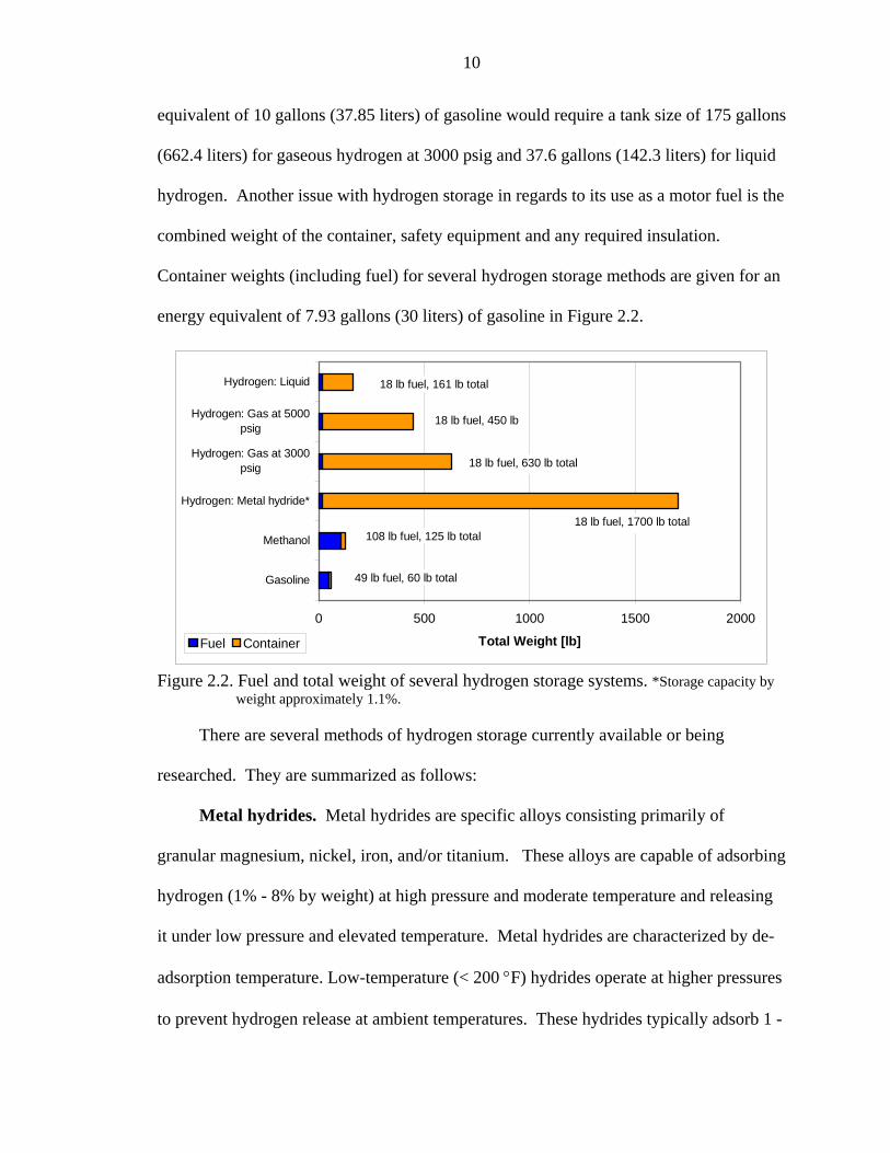
10

equivalent of 10 gallons (37.85 liters) of gasoline would require a tank size of 175 gallons

(662.4 liters) for gaseous hydrogen at 3000 psig and 37.6 gallons (142.3 liters) for liquid

hydrogen. Another issue with hydrogen storage in regards to its use as a motor fuel is the

combined weight of the container, safety equipment and any required insulation.

Container weights (including fuel) for several hydrogen storage methods are given for an

energy equivalent of 7.93 gallons (30 liters) of gasoline in Figure 2.2.

0 500 1000 1500 2000

Gasoline

Methanol

Hydrogen: Metal hydride*

Hydrogen: Gas at 3000psig

Hydrogen: Gas at 5000psig

Hydrogen: Liquid

Total Weight [lb]Fuel Container

18 lb fuel, 161 lb total

18 lb fuel, 450 lb

18 lb fuel, 630 lb total

18 lb fuel, 1700 lb total108 lb fuel, 125 lb total

49 lb fuel, 60 lb total

Figure 2.2. Fuel and total weight of several hydrogen storage systems. *Storage capacity by

weight approximately 1.1%.

There are several methods of hydrogen storage currently available or being

researched. They are summarized as follows:

Metal hydrides. Metal hydrides are specific alloys consisting primarily of

granular magnesium, nickel, iron, and/or titanium. These alloys are capable of adsorbing

hydrogen (1% - 8% by weight) at high pressure and moderate temperature and releasing

it under low pressure and elevated temperature. Metal hydrides are characterized by de-

adsorption temperature. Low-temperature (< 200 °F) hydrides operate at higher pressures

to prevent hydrogen release at ambient temperatures. These hydrides typically adsorb 1 -

11

2 percent of their weight in hydrogen. Higher temperature (> 250 °F) hydrides hold 5 –

10 percent hydrogen by weight, but require significant amounts of heat to attain the

temperatures required to release the stored hydrogen. (Sunatech Inc., 2001).

Metal hydrides provide the safest means of storing hydrogen. Because the

hydrogen is stored in a solid-state media, it cannot be ignited until released. In addition,

the hydrogen is released at low pressures and moderate temperatures; therefore, no

specialized storage tank is required to deal with high pressures or cryogenic temperatures.

Despite these advantages, metal hydrides are undesirable for use in transportation.

Large, heavy, and costly storage units are required to hold equivalent amounts of energy

as current gasoline tanks, as shown in Figure 2.2. Common hydrogen impurities such as

oxygen and water reduce the ability of the tank to store hydrogen as they bond

permanently to the metal. Additionally, vibrations due to typical driving conditions can

result in particle attrition that also reduces the tank’s useful life.

Compressed hydrogen. Compressed hydrogen is the simplest and one of the most

common methods of hydrogen storage and transportation. Even at 10,000 psig, however,

compressed hydrogen contains nearly 8 times less energy per unit volume than gasoline

(not including the energy expended in compressing the hydrogen). Cylinders tend to be

heavy because of the robust construction necessary to withstand the high pressures and

impacts. These factors make compressed hydrogen storage suitable for only short ranged

applications or as a reserve fuel for liquid hydrogen powered vehicles.

Liquefied hydrogen. Liquid hydrogen is formed by cooling hydrogen gas to -423

°F (-253 °C) at atmospheric pressure. Storage of such low temperature fluids is achieved

using a dual-walled cylinder with an evacuated space between the cylinder walls

12

(Dewer’s flask). Due to the relatively high surface to volume ratio typical of the small

tanks used in transportation applications, additional multi-layered radiation insulation

sheets are also employed (Flynn, 1997).

There are several technological challenges that must be overcome in order for

liquefied hydrogen storage to come into widespread use. First is safe tank design to

reduce weight and hydrogen boil off due to heat infiltration. The imperfect insulation of

the inner tank supports, among other factors, causes a typical boil off rate of 3% per day

(Clean Energy Research Center, 2003). Furthermore, improved methods of hydrogen

liquefaction must be developed to reduce LH2 cost. Today, about 30% of the energy

contained in LH2 is consumed by the liquefaction process (Fuel Cell Store, 2003).

Lastly, re-filling stations must be developed such that the public can operate them safely.

Liquefied hydrogen (LH2) is currently the optimum hydrogen storage method for

vehicles in terms of tank size/weight and energy density. LH2 has the highest volumetric

energy capacity of any commercially available storage system being only four times less

than gasoline; and because hydrogen burns more efficiently than gasoline, LH2 tanks are

not necessarily four times the size of typical gasoline tanks for a given vehicle range.

This allows automobile manufactures to continue using current vehicle designs, easing

the transition into a hydrogen economy.

Carbon nanotubes and glass microspheres. Carbon nanotubes store hydrogen in

microscopic surface pores and within the tube structures via adsorption. The mechanism

by which they store and release hydrogen is similar to metal hydrides, however carbon

nanotubes are lighter, cheaper, and are capable of storing 4.2 to 65% hydrogen by weight

(Fuel Cell Store, 2003). Carbon nanotubes are still under research and development and

13

currently store between one and ten percent hydrogen by mass (Clean Energy Research

Center, 2003).

Glass microspheres are currently being researched as a potential hydrogen storage

method. Hydrogen is stored by first warming the tiny glass to increase their surface

permeability and then immersing them in high-pressure hydrogen gas. The spheres are

then cooled, locking the hydrogen inside of the glass balls. Increasing the temperature of

the spheres reverses this process. Experiments to increase hydrogen release rates by

crushing the spheres are also being performed. The key advantage of glass microspheres

is storage at ambient temperature.

The technology exists today for the introduction of hydrogen-powered vehicles;

however, the size, weight, and/or cost limitations imposed on storage systems by the low

energy density of hydrogen must first be overcome. Liquid hydrogen holds the greatest

promise for hydrogen-powered vehicles. These storage systems have the lowest weight

and volume of those commercially available, and with improved tank design and

hydrogen liquefaction methods, the relatively high costs will lessen over time.

Electrolysis of Water

English scientists William Nicholson and Sir Anthony Carlisle first discovered that

the application of an electric current to water produces hydrogen and oxygen in 1800.

The principle of electrolysis was later formulated by Michael Faraday in 1820. Since

then electrolysis has played only a minor role in worldwide hydrogen production;

recently contributing to only 4% of total global production (National Hydrogen

Association, 2004). Current electrolytic hydrogen production is limited to low-cost

electricity sources such as hydroelectric or small-scale onsite generation in which purity

is essential.

14

The importance of electrolysis in a future hydrogen economy is two fold: First, as

discussed previously, electrolysis powered by wind or the ammonia water combined

power/cooling cycle is projected to be the most cost efficient hydrogen production

method by 2020. Second, it provides a practical link between hydrogen and renewable

resources through electricity generation. In this manner, electrolysis can indirectly utilize

any energy source that can be used to produce electricity. Furthermore, when powered by

electricity generated from renewable sources of energy, electrolysis does not require

fossil fuels and has zero polluting emissions.

Process Description

Electrolysis is defined by McMurray and Fay as the use of an electric current to

drive a non-spontaneous chemical reaction (1998). Electrolysis of water consists of a

pair of oxidation/reduction reactions driven by a DC voltage applied across two

electrodes as described by equations 2.1a – 2.1c.

Cathode: −− +→+ OHHeOH 222 22 (2.1a)

Anode: −− ++→ eOHOOH 2212 22 (2.1b)

Overall: 222 2

1 OHOH +→ (2.1c)

Water is reduced at the cathode to form hydrogen gas and hydroxide ions ( −OH ). The

−OH ions migrate toward the anode where they are oxidized to form oxygen, water, and

two free electrons. The free electrons are then attracted to the positively charged cathode,

thus completing the circuit. A schematic of a simple electrolyzer and the overall

electrolysis process is given in Figure 2.3.

Each electrode is isolated from the other with an ion-conducting diaphragm to keep

the product gases separate; and an electrolyte is used to make the solution conductive.

15

The electrolyte is chosen such that its reduction and oxidation potentials are less than that

of water. In this manner, the electrolyte is conserved because it acts only as an ion-

conducting substance.

Figure 2.3. Process diagram of a simple alkaline electrolyzer (adapted from Mirabal)

Energy and Efficiency

The voltage required for reversible or isentropic electrolysis is proportional to

Gibb’s free energy of reaction as defined by Faraday’s Law:

nFEG −=∆ (2.2)

where ∆G is Gibb’s free energy of reaction n is the number of electrons transferred in the reaction F is Faraday’s constant, mol

Coulombs410648531.9 ×

E is the cell voltage

A negative sign is included on the right hand side of Equation 2.2 because by

convention voltage input is considered negative (McMurray and Fay, 1998). The

spontaneity of a given reaction is determined by the sign of the Gibbs free energy of

reaction (from hereon referred to as GFR). GFR is positive for non-spontaneous

reactions and negative for spontaneous ones. For water at standard temperature and

pressure, (25 °C and 1 atm), the GFR is 50,941 Btu/lbmH2 (14.93 kW-h/lbmH2) and the

corresponding reversible voltage is 1.23 V. The electrical energy required to drive the

16

electrolysis reaction is equal to the GFR (Casper, 1978). The enthalpy of reaction (higher

heating value) of hydrogen, however, is 61,451 Btu/lbm (18.01 kW-h/lbmH2).

Conservation of energy dictates that the remaining 10,510 Btu/lbm (48.89 kJ/mol) must

be supplied as heat. For a reversible process, this heat would be obtained from the

surroundings, and the electrolyzer would double as a refrigeration unit.

The second law of thermodynamics states that entropy always increases for any real

process. Entropy production in electrolysis increases the required cell voltage as

described by equation 2.3.

PTEnFTnFESTGH ⎟⎠⎞

⎜⎝⎛∂∂

+−=∆+∆=∆ (2.3)

where pP T

EnFTGS ⎟

⎠⎞

⎜⎝⎛∂∂

=⎟⎠⎞

⎜⎝⎛∂∆∂

=∆ from Faraday’s Law

The entropy produced is liberated as heat, which supplies the additional 10,510 Btu/lbm

necessary to form hydrogen. The voltage required for isothermal electrolysis (defined as

the thermoneutral voltage) is 1.47V. This result is obtained by replacing ∆G in Equation

2.2 by the HHV of hydrogen. In reality, the thermoneutral voltage is the lowest that can

possibly be achieved.

Real electrolyzers require greater than the thermoneutral voltage due to additional

overvoltages independent of the entropy generation. Overvoltage is defined as the

difference between the applied voltage and the reversible 1.23V and is proportional to the

amount of current passed through the cell (Casper, 1978). These overvoltages include:

ohmic resistance of the electrolyte, concentration polarization (changes in the

concentration of H+ or O2+ or water near the electrodes), voltage gradients at the

electrode/electrolyte interface due to the slowness of reaction (proportional to cell

17

operating temperature), and wire and component resistance (typically about 2% of total

loss) (Casper, 1978). The primary source of electrolyte resistance is the formation of

vapor bubbles on the electrodes (Wendt, 1990). Additional energy losses occur (typically

5% of total energy consumption) within each subsystem including AC to DC

rectification, cooling water system, feed water pumps, and electrolyzer pumps (if

necessary) (Casper, 1978).

The majority of electrolyzer manufacturers have taken steps to reduce these

overvoltages. Concentration polarization can be avoided by adequate mixing of the

electrolyte through circulation or by natural gas lift. One method developed to reduce

electrolyte resistance is zero gap cell geometry in which porous electrodes are pressed on

either side of the diaphragm, forcing the product gases to leave from the rear (Wendt,

1990). Another technique is to increase the cell operating temperature and pressure in

order to speed up reaction kinetics and reduce electrolyte resistance. However, this also

enhances corrosion of the electrodes and shortens operating lifetime.

The figures of merit measuring electrolyzer performance are current,

electrochemical, and thermal efficiencies. Current efficiency measures deviation from the

hydrogen yield predicted by Faraday’s law at 1.47 V and 1000 A-h due to extraneous

electrode reactions (Casper, 1978). For most electrolyzers, this number approaches

100%. Electrochemical efficiency is defined as the reversible voltage divided by the

operating voltage. The maximum electrochemical efficiency under isothermal conditions

is 83.7%. Thermal (1st law) efficiency is the ratio of the isothermal voltage to the

operating voltage or the HHV of hydrogen divided by electricity input as given by

Equation 2.4.

18

Elec

H

act

thElec E

HHV

VV 2==η (2.4)

Using this definition of efficiency, ideal electrolysis operates at an apparent 120%

efficiency. Thermal efficiency is the most widely used figure of merit by electrolyzer

manufactures, therefore any given efficiency will be thermal efficiency. Commercial

electrolyzers currently operate at efficiencies (excluding subsystems) of up to 85%

(Stuart Energy, 2004)

Electrolyzer Designs

Electrolyzers are typically classified by their electrolyte; the most common of

which is alkaline/water (Casper, 1978). Others include solid polymer (SPE), seawater,

and solid oxide; descriptions of which are given by Casper (1978).

Alkaline/water electrolyzers typically operate with a 30% potassium hydroxide

(KOH) solution at relatively low temperatures of 158 – 212 °F (70 – 100 °C). There are

two varieties of alkaline/water electrolyzer: monopolar (tank-type) and bipolar (filter-

press). A summary of each type highlighting the unique advantages and drawbacks of

each is given below:

Monopolar or tank-type cells are constructed as an alternating set of anodes and

cathodes connected electrically in parallel and hung vertically from gas collectors into a

tank of electrolyte. Mixing of the electrolyte is achieved through simple gas lift. The

cathodes are normally surrounded by a diaphragm to prevent the mixing of gases. This

arrangement results in individual tanks operating at low voltages (typically 1.9 – 2.5 V)

and high currents (Casper, 1978).

Bi-polar or filter-press electrolyzers are characterized by the stacked design of the

cells. In this configuration, one side of an electrode serves as the cathode and the other as

19

the anode of an adjoining cell. Electrodes are connected in series such that a desired

operating voltage is achieved by increasing the total number of cells. The geometries of

these cells are relatively thin; therefore, a pump is required to circulate the electrolyte

through the cells. Bi-polar cells typically operate at lower current levels due to higher

operating voltage. Table 2.4 lists the pros and cons of each alkaline/water electrolyzer

design.

Table 2.4. Advantages and disadvantages of monopolar and bipolar electrolyzers Advantages Disadvantages

Monopolar

• Require relatively few, inexpensive parts

• Easily maintained – individual cells can be isolated for repair with minimum plant downtime

• No pumps required for electrolysis circulation

• Unable to operate at high temperatures because of heat loss from large surface areas

• Bulky design requires greater space per unit hydrogen produced

• Tanks are difficult to design for pressurized electrolysis

• Relatively high voltage losses and non-uniform current density distribution result from long current paths (Wendt)

Bi-polar

• Compact design • Capable of operating at

high pressures and temperatures

• Lower ohmic resistance and energy losses

• Requires precise fabrication tolerances and additional gaskets due to sealing problems

• Maintenance is more difficult – if one cell fails, the entire cell must be shut-down and dismantled

One of the largest electrolytic hydrogen production plants in North America was

built by Cominco, Ltd. in British Columbia, Canada. Before being shut down due to high

electricity costs, the plant produced 41 tons/day of hydrogen with 3,229 individual tank-

20

type cells operating at 2.1 V (70% efficient) (Casper, 1978). Since that time, most

manufactures have adopted the more efficient bi-polar design (Wendt, 1990).

Hydrogen Liquefaction

Liquid hydrogen was first produced by James Dewar in 1898; however, up until the

mid 1940s to mid 1950s it remained nothing more than a laboratory curiosity (Flynn,

1997). In the late 1950s, the US Air Force began producing substantial amounts of LH2

for its top secret “Bear” Program. Under contract to the Air Force, Air Products and

Chemicals, Inc., constructed three production plants code named “Baby Bear,” “Mama

Bear,” and “Papa Bear” to support Air Force aerospace programs. The largest of these

was Papa Bear, which produced 30 tons/day in 1959 (Flynn, 1997). Today, total annual

production of LH2 in North America is nearly 300 tons/day (Drnevich, 2003).

Demand for large-scale liquid hydrogen production was initially sparked by the

Apollo space program. Liquid hydrogen demand has increased and simultaneously

shifted since the 1960s from aerospace to research and industry. Flynn reports that

aerospace accounted for only 20% of total liquid hydrogen demand in 1990 (1997). This

trend is expected to continue with the onset of a hydrogen economy including the

advancement of fuel cell powered vehicles and the development of improved storage

systems.

Hydrogen production companies are already taking advantage of the higher energy

density of LH2 vs. gaseous hydrogen to effectively reduce distribution costs. Where a

full tube-trailer of gaseous hydrogen contains approximately 300 kg of deliverable

gaseous hydrogen, a comparably sized liquid hydrogen trailer carries 4000 kg (Drnevich,

2003). Another benefit of liquefying hydrogen is the ultra high purity that results from

the majority of trace impurities condensing out. High energy density and purity make

21

liquid hydrogen a well-suited fuel for hydrogen fuel cell powered vehicles in an emerging

hydrogen economy; giving equivalent performance and driving range as today’s gasoline

and diesel automobiles.

Process Description

Hydrogen, like all gases, is liquefied by cooling it to its boiling point, -423 °F

(-252.8 °C). There are several liquefier designs; all of which are derived from the simple

Linde cycle shown in Figure 2.4 and follow the same general process.

The incoming gas is compressed isothermally from 1 to 2 on the diagram to a

relatively high pressure. Heat is rejected to a cold return stream and the cooled gas is

expanded from 3 to 4 on the diagram to atmospheric pressure and cryogenic

temperatures. The two-phase flow that results is separated in a flash tank where the

liquid yield is drawn off and collected and the remaining gas absorbs heat from the

warmer high-pressure stream before it’s recycled back to the compressor. The expansion

can be accomplished using either a Joule-Thompson (expansion or throttling) valve or a

work-extracting device.

Isenthalpic vs. isentropic expansion

Joule-Thompson expansion is modeled as isenthalpic by neglecting potential and

kinetic energy changes as well as heat transfer (insulated valve). The effect that a change

in pressure has on the temperature for an isenthalpic process is described by the Joule-

Thompson coefficient given by Equation 2.5. A negative value indicates a temperature

increase with expansion; a positive value indicates a temperature decrease.

TphJT p

hhT

pT

⎟⎟⎠

⎞⎜⎜⎝

⎛∂∂

⎟⎠⎞

⎜⎝⎛∂∂

−=⎟⎟⎠

⎞⎜⎜⎝

⎛∂∂

=µ (2.5)

22

By substituting the definition of specific heat at constant pressure, p

p Thc ⎟⎠⎞

⎜⎝⎛∂∂

= ,

pT T

vTvph

⎟⎠⎞

⎜⎝⎛∂∂

−=⎟⎟⎠

⎞⎜⎜⎝

⎛∂∂ , and the volumetric coefficient of thermal expansion,

pTv

v⎟⎠⎞

⎜⎝⎛∂∂

=1β , the Joule-Thompson coefficient is given in its more useful form:

{ }vTc p

JT 11−= βµ (2.6)

Equation 2.6 demonstrates that the sign of the Joule-Thompson coefficient depends

only on the product of βT . At a given pressure, the volumetric coefficient of thermal

expansion and the specific volume are functions of temperature only. Consequently, a

temperature can be identified at which 0=JTµ . This point is known as the inversion

temperature; and represents the maximum temperature at which a gas can be cooled by

isenthalpic expansion.

Most practical liquefaction systems use an expansion valve to produce low

temperatures (Barron, 1985). In the case of hydrogen, however, the maximum inversion

temperature at STP is well below ambient (-90.7 °F (-68 °C)). Additional energy is

required to pre-cool the hydrogen below its inversion temperature for isenthalpic

expansion to be effective.

Expansion in a work-extracting or work-producing device is commonly modeled as

adiabatic and reversible (i.e. isentropic). This process is represented by an isentropic

expansion coefficient, Equation 2.7.

ss p

T⎟⎟⎠

⎞⎜⎜⎝

⎛∂∂

=µ (2.7)

23

By substituting the Maxwell relation ps s

vpT

⎟⎠⎞

⎜⎝⎛∂∂

=⎟⎟⎠

⎞⎜⎜⎝

⎛∂∂ , applying the chain rule, and using

the definitions defined previously, the isentropic expansion coefficient is given in the

same terms as the Joule-Thompson coefficient:

( )vTc p

s βµ 1= (2.8)

Equation 2.8 shows that the isentropic expansion coefficient is always positive

(the temperature always decreases with pressure) because the coefficient of thermal

expansion (β ) for gases is always positive (Hands, 1986). This conclusion can also be

arrived at intuitively by considering conservation of energy. If work is extracted from a

fluid adiabatically, the internal energy and hence temperature must decrease.

Thermodynamically, isentropic expansion is more desirable than isenthalpic

expansion. The T-S diagram in Figure 2.5 shows that an isentropic expansion will

always result in a lower final temperature than isenthalpic expansion.

s

T

1

2s 2h

p1

p2

T2h

T2s

h = const

Figure 2.5. T-S diagram comparing isenthalpic and isentropic expansion

Practically, however, expansion devices cannot tolerate an appreciable amount of liquid.

For this reason, expansion valves are necessary in all liquefaction systems (Barron,

1985). The Claude cycle discussed later seeks to combine the benefit of isentropic

24

expansion with the necessity of isenthalpic expansion as an efficient means of liquefying

hydrogen.

Ortho/para conversion

Another challenge to simple liquefaction systems is the unique sub-atomic structure

of hydrogen. Hydrogen exists in two different molecular forms: ortho-hydrogen and

para-hydrogen. Each form is distinguished by the relative spins of its protons. The

protons of ortho-hydrogen spin in the same direction whereas the proton spins of para-

hydrogen oppose one another. Hydrogen at STP (i.e. normal hydrogen) is composed of

74.928% ortho and 25.072% para hydrogen. At the normal boiling point of hydrogen

(-423 °F (-293.4 °C) at 1 atm) the equilibrium ortho/para composition is .21%/99.79%

(Flynn, 1997).

Converting from ortho to para hydrogen is an exothermic process, releasing 302.4

Btu/lbm (703.3 kJ/kg) of heat at STP (Barron, 1985). The conversion process is

relatively slow and the resident time of the hydrogen within the liquefier is short, so the

liquid hydrogen essentially retains its room temperature ortho/para composition.

Conversion gradually takes place in the storage tank resulting in boil-off losses because

the heat of conversion exceeds the latent heat of vaporization (190.5 Btu/lbm or 443

kJ/kg) (Barron, 1985). The heat liberated during the conversion process is sufficient to

evaporate nearly 70% of the original amount of hydrogen liquefied (Flynn, 1997).

Storage time is a major issue with regard to liquid hydrogen as a motor fuel so it is

important that the boil-off losses due to ortho/para conversion are minimized.

Catalysts are used to speed up the conversion reaction allowing the heat to be

absorbed by the liquefier. This alleviates boil-off in storage, but at a penalty to the

25

overall efficiency of the liquefier. The most efficient method of conversion is to have the

process take place simultaneously as the hydrogen is cooled. This is not possible in

practice but can be simulated by cooling the hydrogen to liquid nitrogen temperatures

(-320.4 °F or –195.6 °C) and passing it through an adiabatic converter then repeating this

procedure in a step-wise manner (Flynn, 1997). Common materials proven effective as

catalysts are ferric hydroxide gel, chromic oxide on alumina particles, and nickel silicate;

all of which provide nearly 100% conversion to para hydrogen within a few minutes

(Hands, 1986).

Claude cycle

The Claude cycle is the most commonly used system for large-scale hydrogen

liquefaction (Hands, 1986). The performance of the cycle is enhanced by pre-cooling the

compressed hydrogen gas to liquid nitrogen (LN2) temperatures. Adding catalysts in the

LN2 and LH2 baths provides a convenient and effective means of absorbing the heat of

conversion. Figure 2.6 shows a schematic of this variation of the Claude cycle with

labeled state points and flow paths.

Hydrogen gas typically enters the cycle at 1 atm and 80.6 °F (27 °C) (state 1). It is

compressed isothermally (isothermal compression is achieved through multistage

compression with inner-cooling and after-cooling) to state 2, typically 20 to 40 atm

(Barron, 1985). The pressurized gas then exchanges heat with the return hydrogen and

nitrogen streams (state 2a) before entering the LN2 bath where it is cooled to -320.4 °F

(-195.6 °C) and where the first step of ortho/para conversion occurs (state 2b). At this

temperature, the equilibrium concentration of para hydrogen (assuming 100%

conversion) is 50%.

26

Compressor

Wc

21

L

Liquid hydrogenbath

8

g

e

7

Catalyst bed 2

5

4

2a 2b

Catalyst bed 1

We

10

Expander

10a

3

Liquid nitrogen bath

9a9b

Figure 2.6. Claude cycle with liquid nitrogen pre-cooling and ortho/para catalyzation

It is desirable to perform the maximum amount of conversion at this stage because liquid

LN2 is less expensive to produce then liquid oxygen. The hydrogen is further cooled in

the first heat exchanger to state 3. At this point, a portion of the flow (typically 60 to

80%) is diverted and expanded isentropically through a work-extracting device and used

to pre-cool the compressed hydrogen. The expander work is used to offset the

compressor work requirement, increasing the overall cycle efficiency. The remaining

flow continues through the next two heat exchangers and into the liquid receiver. Here

the flow streams are halved and throttled through expansion valves. The liquid yield from

the first stream (state 9a) is collected in the receiver and used sacrificially to absorb the

heat of conversion from the second catalytic bed. The second stream (state 9b) is passed

27

through the catalytic bed where it is ideally converted to 99.789% para hydrogen and

extracted.

Ammonia-Water Combined Power/Cooling Cycle

The ammonia-water combined power/cooling cycle proposed by Goswami (1995)

utilizes a binary ammonia/water working fluid to produce both power and refrigeration.

The cycle is a combination of an ammonia-water refrigeration system and an ammonia-

based Rankine cycle.

An ammonia-water mixture is used because of its desirable thermodynamic

properties. Binary mixtures have varying boiling points depending on the concentration

of the more volatile species. This characteristic gives a good thermal match with a

sensible heat source, thereby reducing the irreversibility associated with heat transfer

(Hasan, Goswami, 2003). Additionally, the low boiling point of ammonia allows the

utilization of low temperature heat sources such as low-grade waste heat from industrial

processes, solar water heaters, and geothermal sources. In a theoretical investigation

performed by Tamm et al., the cycle is shown to operate with heat source temperatures as

low as 116.6 °F (47 °C) albeit with low first law efficiency (~ 5%). When operating with

a heat source temperature of 224.6 °F (107 °C) and idealized parameters, however,

second law efficiencies greater than 65% are possible (2003).

The unique ability of this cycle to produce both power and refrigeration gives rise

to two advantages for use in a hydrogen economy. First, the cycle can utilize low-grade

renewable heat sources such as that available from inexpensive flat plate solar collectors

to produce the power needed to drive an electrolyzer and liquefier. Second, the cooling

produced by the cycle can be used to pre-cool hydrogen prior to liquefaction, thereby

28

reducing the power requirement of the compressor. In this manner renewable energy

source utilization is improved compared to technologies such as wind or P.V.

electrolysis.

Process Description

Figure 2.7 gives a schematic of the cycle showing state points and flow paths.

CHWSCHWR

HHWS

HHWR

Cooler

Vapor Generator

Absorber

Expander

RectifierColumn

Superheater

Recovery Heat Exchanger

HHWS HHWR

SolutionPump

CWS CWR

CWR

CWS

Figure 2.7. Combined cycle flow diagram

The fluid leaves the absorber at state 1 as a saturated solution at the cycle low pressure

with a relatively high ammonia concentration. It is pumped to the system high pressure

(state 2) before traveling through the recovery heat exchanger where it absorbs heat from

the weak solution returning to the absorber. The solution is then partially boiled in the

vapor generator by the heat source producing saturated ammonia vapor and relatively

weak concentration ammonia-water saturated liquid. The weak solution leaves the vapor

generator at state 4 and rejects heat to the high concentration stream before it is throttled

29

to the system low pressure and sprayed into the absorber. The rectifier cools the

saturated ammonia vapor to condense out any remaining water. The vapor is then

superheated to state 7 and expanded to produce work. The sub-ambient exhaust vapor

(state 8) provides refrigeration before returning to the absorber where it is re-absorbed

into the weak solution. The heat of condensation is rejected to the low-temperature source

and the cycle repeats.

The power output and cooling capacity of the cycle under given operating

parameters is highly dependent on the expander efficiency. Irreversibilties due to friction

and leakage decrease the amount of work extracted from the fluid. Because less work is

extracted, the expander exhaust temperature is higher and the cooling capacity is reduced.

Losses in the expander have the greatest impact on the overall cycle efficiency (Tamm et

al., 2003), so it is important to select an optimal design.

The main criteria for expander selection are operating pressures and temperatures,

flow rate of ammonia vapor and material compatibility with ammonia. Ammonia is a

corrosive substance that reacts with metals such as copper, brass, and bronze, all of which

are commonly used as bearing or bushing material. The expander selected for use in the

combined cycle must be sized correctly for the flow rate and for the operating pressure

ratio for maximum power production and refrigeration capacity. It must also be

constructed out of steel, aluminum, or any other material compatible in an ammonia

environment.

Expander Design

An expansion device extracts mechanical energy from a fluid by expanding it from

a high to a low pressure and converting it into shaft work. Various expander designs

using unique expansion methods exist throughout industry. These designs can be

30

organized into two categories, positive-displacement and turbo-machinery, based on the

method of fluid displacement.

Positive-displacement expanders

Positive-displacement machines such as reciprocating and rotary piston, rotary

vane, and screw operate by expanding a fixed volume of fluid per oscillation. Torque

pulsation is a common phenomenon due to the inherent discontinuity associated with the

finite number of pistons or lobes and fixed displacement. Reliability is an issue with

positive-displacement machines because of a greater number of moving parts (i.e. piston

linkages, sliding vanes); and in the case of pistons, a lubrication system to reduce leakage

encountered in the gap between the moving seals and volute.

Turbo-machinery

Turbo-machinery, comprised of axial and radial flow turbines, utilizes the pressure

differential across a series of radial blades to provide a “lift” force to turn the rotor,

thereby producing shaft work. In this manner, a continuous power output is provided.

Reliability is improved over positive-displacement expanders because the rotor is the

only moving part.

Turbines are designed with a clearance between the blade tips and the volute to

allow free rotation; however, leakage at the tips (windage loss) is the primary cause of

irreversibility in the expansion process. Blade tip clearances remain approximately

constant for varying turbine size. As turbine size is decreased, the loss due to windage as

a percentage of the work output becomes increasingly significant. For this reason,

positive-displacement expanders are more suited for small-scale operations.

The amount that the blade tip clearances can be reduced is limited by the

centrifugal force and/or thermal expansion of the blade material. Typical turbine

31

operating speeds range from a few thousand up to tens of thousands RPM. Centrifugal

force is dependent on blade tip speed, which is function of the RPM and the rotor

diameter. As a result, larger turbines suffer greater radial blade deformation and are less

suited for blade tip clearance reduction.

Scroll compressor/expander

The scroll compressor was first invented by Lèon Creux in 1905 (Gravesen and

Henriksen, 2001). Commercial interest in the technology wasn’t strong until the

introduction of computer numerically controlled (CNC) machines in the 1970s. CNC

machines provided the basis for machining the precise elements needed for a scroll

compressor to operate efficiently and quietly (Copeland corp., 2001).

A scroll compressor consists of two identical spiral elements assembled with a 180°

phase difference. During operation, one scroll remains stationary and the other is

attached eccentrically to a motor shaft. This configuration allows the scroll to rotate in an

orbiting motion within the fixed scroll. The phase difference between the two scrolls is

maintained using an anti-rotation device, typically an Oldham coupling (Copeland corp.,

2001).

The fluid flow path within a scroll compressor or expander is described by Figure

2.8. As the rotating scroll (green) orbits about the fixed scroll (red), the outer periphery

forms a line of contact with the fixed scroll, capturing a crescent shaped volume of gas

(step 1). The gas is forced toward the center discharge port in steps 2 thru 5 and

compressed due to the decreasing volume of the crescents. This is indicated by the

brilliance of the yellow color representing the gas pocket. Because several of these gas

pockets are being compressed simultaneously, as depicted in step 6, torque pulsation

32

common with other positive-displacement machines is low. Scrolls compressors have

been widely adopted by the HVAC industry because of the advantages they offer,

including: simplistic design (i.e. fewer moving parts), low friction, low torque pulsation,

and compliance.

Figure 2.8. Flow path of a single fluid pocket through a scroll compressor (Adapted from

Gravesen and Henriksen, 2001)

Because of their unique geometry, scrolls do not require valves or valve actuators;

furthermore, there are no linkages or sliding vanes. The relative rolling motion of the

contact points offers less resistance than sliding friction. Additionally, the rolling

contacts provide a seal such that large volumes of oil used as a sealant are not required

and leakage is reduced (Copeland corp., 2001). Continual compression process of the

scroll results in a smoother power output and consequently less noise and vibration than

piston-type devices. Compliance mechanisms balance the dynamic pressure and

centrifugal forces in order to maintain proper sealing. These loading mechanisms correct

tolerances as the scroll surfaces wear and allow the scroll elements to separate slightly in

the axial or radial directions in response to a sudden pressure spike (axial compliance) or

6.

3. 4. 5.

2. 1.

33

the presence of small amounts of debris or liquid (radial compliance). Taken together,

these attributes contribute to the fact that scroll compressors typically have 10% higher

mechanical efficiencies than comparably sized piston compressors (Wells, 2000) and less

leakage than other compressors in its class (Schein and Radermacher, 2001).

Literature suggests the potential use of a scroll compressor as a high efficiency

expander (Wells, 2000). Copeland® compressors have been used successfully as

expanders with R-134A and R-245FA refrigerants as the working fluid. Efficiencies over

70% were demonstrated when operated with pressure ratios between three and five

(Warner, Wayne – Copeland Corporation, Personal Conversation, 10 May 2004). Scroll

expanders have also been utilized in an organic Rankine micro combined heat and power

system patented by Yates et al. in 2002 (US Patent and Trademark Office, 2002).

5 kW Prototype

The applicability of the ammonia-water combined cycle for small scale power

generation utilizing low temperature heat sources is currently being studied at the

University of Florida’s Energy Research Park. A prototype producing 5 kW of electrical

power has been designed and is under construction.

Heat source and sink. The low-temperature heat source is simulated using a

liquid-propane-fired boiler to heat water to 180 °F. The heat sink for the cycle is cooling

water, which is continually circulated through a 500,000 btu/h cooling tower.

Temperature control is accomplished using a combination of 3-way automatic control

valves and several shell and tube heat exchangers.

Absorber and solution pump. The absorber is a falling-film type. This design

offers a combination of sufficiently high heat transfer rates and large surface areas for

34

absorption. The fluid leaving the absorber is saturated, therefore no net positive suction

head (NPSH) is available for the pump, leading to cavitation. For this reason, a roller-

type positive-displacement pump is used.

Vapor generator and rectifier. The vapor generator and rectifier are integrated as

a single unit such that no separator is required. The vapor generator is a shell and tube

heat exchanger with hot water on the tube side; the rectifier is a packed column. As the

ammonia bubbles out of solution, it travels through the rectifier and the remaining

effluent drips back down into the vapor generator where it is re-boiled.

Electricity production and cooling capacity. The maximum power output of the

expander is 5.6kW. This work is used to run an electric generator that produces 200 Vrms

single phase AC at 400 Hz. A frequency converter switches the frequency from 400 to

60 Hz required by the electrolyzer. The maximum equivalent cooling capacity of the

system is 1.25 kW; this is demonstrated by cooling a fixed volume of water.

35

CHAPTER 3 ANALYSIS METHODOLOGIES

This chapter outlines the analytical procedure developed to find the expected

energy requirements for electrolysis and hydrogen liquefaction, as well as the heat and

work interactions of the combined cycle at steady state. An analysis on impact of the

combined cycle expander efficiency on the cooling capacity and the liquid hydrogen

yield is discussed as motivation for an experimental study.

Hydrogen Energy Requirements

Electrolysis of Water

The electrolyzer model used in this study is based on the Stuart Energy

Vandenborre IMET® Electrolyzer. The IMET® is selected for two reasons: its relatively

simple design due to pump-less electrolyzer circulation, and its high thermal efficiency

(operating at a cell voltage of approximately 1.7V) (Stuart Energy, 2004). It utilizes an

alkaline electrolyte in a filter-press arrangement and can deliver hydrogen at pressures of

up to 363 psi (25 atm), which reduces the compressor power required for liquefaction.

The analysis determines the total electrolyzer power consumption per unit mass hydrogen

produced including the power required to operate the sub-systems of the electrolyzer,

namely the cooling water system, feed water / deionization system, and AC/DC rectifier.

Equation 3.1 defines the thermal efficiency of the electrolyzer, assuming 100%

current efficiency (Casper 1978).

Elec

H

actual

tnth E

HHV

VV

Elec

2==η (3.1)

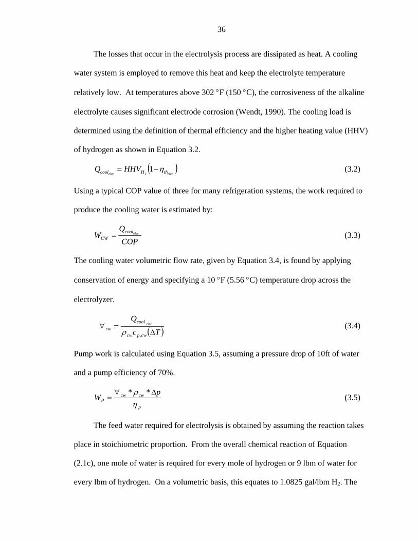
36

The losses that occur in the electrolysis process are dissipated as heat. A cooling

water system is employed to remove this heat and keep the electrolyte temperature

relatively low. At temperatures above 302 °F (150 °C), the corrosiveness of the alkaline

electrolyte causes significant electrode corrosion (Wendt, 1990). The cooling load is

determined using the definition of thermal efficiency and the higher heating value (HHV)

of hydrogen as shown in Equation 3.2.

( )elecelec thHcool HHVQ η−= 1

2 (3.2)

Using a typical COP value of three for many refrigeration systems, the work required to

produce the cooling water is estimated by:

COPQ

W eleccoolCW = (3.3)

The cooling water volumetric flow rate, given by Equation 3.4, is found by applying

conservation of energy and specifying a 10 °F (5.56 °C) temperature drop across the

electrolyzer.

( )Tc

Q

cwpcw

coolcw

elec

∆=∀

,ρ (3.4)

Pump work is calculated using Equation 3.5, assuming a pressure drop of 10ft of water

and a pump efficiency of 70%.

p

cwcwP

pW

ηρ ∆∀

=**

(3.5)

The feed water required for electrolysis is obtained by assuming the reaction takes

place in stoichiometric proportion. From the overall chemical reaction of Equation

(2.1c), one mole of water is required for every mole of hydrogen or 9 lbm of water for

every lbm of hydrogen. On a volumetric basis, this equates to 1.0825 gal/lbm H2. The

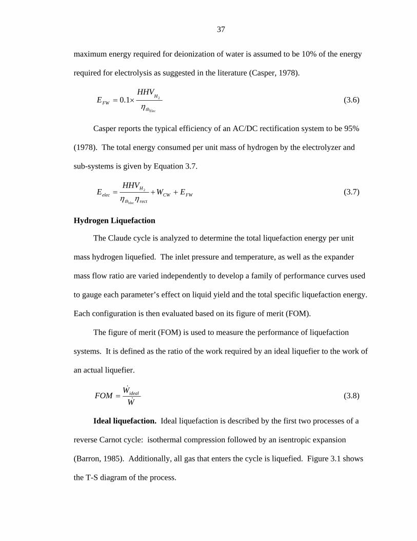
37

maximum energy required for deionization of water is assumed to be 10% of the energy

required for electrolysis as suggested in the literature (Casper, 1978).

Electh

HFW

HHVE

η21.0 ×= (3.6)

Casper reports the typical efficiency of an AC/DC rectification system to be 95%

(1978). The total energy consumed per unit mass of hydrogen by the electrolyzer and

sub-systems is given by Equation 3.7.

FWCWrectth

Helec EW

HHVE

elec

++=ηη

2 (3.7)

Hydrogen Liquefaction

The Claude cycle is analyzed to determine the total liquefaction energy per unit

mass hydrogen liquefied. The inlet pressure and temperature, as well as the expander

mass flow ratio are varied independently to develop a family of performance curves used

to gauge each parameter’s effect on liquid yield and the total specific liquefaction energy.

Each configuration is then evaluated based on its figure of merit (FOM).

The figure of merit (FOM) is used to measure the performance of liquefaction

systems. It is defined as the ratio of the work required by an ideal liquefier to the work of

an actual liquefier.

WW

FOM ideal&

&= (3.8)

Ideal liquefaction. Ideal liquefaction is described by the first two processes of a

reverse Carnot cycle: isothermal compression followed by an isentropic expansion

(Barron, 1985). Additionally, all gas that enters the cycle is liquefied. Figure 3.1 shows

the T-S diagram of the process.

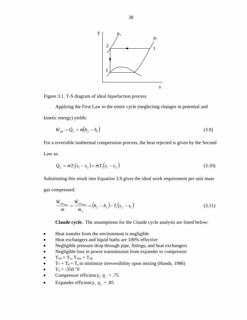
38

p1

p2

1 2

f

T

s

Figure 3.1. T-S diagram of ideal liquefaction process

Applying the First Law to the entire cycle (neglecting changes in potential and

kinetic energy) yields:

( )1hhmQW fCnet −+= &&& (3.9)

For a reversible isothermal compression process, the heat rejected is given by the Second

Law as:

( ) ( )fC ssTmssTmQ −=−= 11211 &&& (3.10)

Substituting this result into Equation 3.9 gives the ideal work requirement per unit mass

gas compressed.

( ) ( )112 ssThhm

Wm

Wff

f

netnet idealideal −−−==&

&

&

& (3.11)

Claude cycle. The assumptions for the Claude cycle analysis are listed below:

• Heat transfer from the environment is negligible • Heat exchangers and liquid baths are 100% effective • Negligible pressure drop through pipe, fittings, and heat exchangers • Negligible loss in power transmission from expander to compressor • T10 = T1, T10a = T2b • T7 = T8 = Te to minimize irreversibility upon mixing (Hands, 1986) • T3 = -350 °F • Compressor efficiency, cη = .75 • Expander efficiency, eη = .85

39

• Electrolyzer produces 100% pure normal hydrogen (74.928% ortho, 25.072% para) • Ortho/para conversion proceeds to equilibrium within the liquid nitrogen (LN2)

bath

In this model, ortho-para conversion takes place in two isothermal stages. First, the

gas is cooled to LN2 temperatures (-320.4 °F, -195.6 °C) and passed over a catalyst bed.

Equilibrium concentration of para hydrogen at this temperature is 50.5%. This

corresponds to an approximate 25.43% conversion from normal hydrogen, releasing

75.28 btu/lbm (175.1 kJ/kg) of heat (heat of conversion at –320.4 °F is 296.07 btu/lbmH2

(688.62 kJ/kg)). The second stage takes place in the liquid hydrogen-receiving tank at

liquid hydrogen (LH2) temperatures (-423 °F, -252.8 °C). The heat of conversion from

normal to para hydrogen at -423 °F is 302.38 btu/lbm (703.3 kJ/kg). The heat released in

proceeding from 50.5% to 99.789% para hydrogen is 134.56 btu/lbm (312.97 kJ/kg).

The liquid yield of the cycle per unit mass hydrogen compressed is found by

applying the First Law to a control volume including the three heat exchangers, Joule-

Thompson valve, and liquid hydrogen-receiving tank (subscripts refer to Figure 2.6).

( ) ffeeafeebCf hmhmhmmhmhmHm &&&&&&& ++−=++∆ 1022 (3.12)

where 2CH∆ is the heat of conversion in the second stage m& is the inlet mass flow rate of hydrogen

Dividing by m& , introducing the liquid yield per unit mass hydrogen compressed,

mm

y f

&

&= , and the expander mass flow ratio,

mm

x ee &

&= , and solving for y gives:

( )210

3

210

210

Cfa

eee

Cfa

ba

Hhhhhx

Hhhhh

y sad

∆+−

−+

∆+−−

=η

(3.13)

The amount of liquid nitrogen required to pre-cool the compressed hydrogen and absorb

40

a portion of the heat of conversion is determined by applying the First Law to a control

volume encompassing the three-stream heat exchanger, liquid nitrogen receiver and the

control volume from the previous analysis.

( ) ffeeCNfANeeCfC hmhmhmhmmhmhmhmHmHm &&&&&&&&&& +++−=+++∆+∆22 10221

Dividing by m& , defining the mass ratio of liquid nitrogen to compressed hydrogen as

mm

z N

&

&2= , and solving for z yields Equation 3.14

AC

Cf

AC

eee

ACAC

C

hhHhh

yhhhh

xhhhh

hhH

z s

ad −

∆+−+

−

−−

−−

+−

∆= 21031021 η (3.14)

where 1CH∆ is the heat of conversion in the first stage

Dividing Equation 3.14 by the liquid yield, y, gives the hydrogen requirement in terms of

unit mass hydrogen liquefied. Based on the literature, the specific energy required to

produce liquid nitrogen is assumed 766.82 btu/lbm-N2 or 0.225 kW-h/lbm-N2 (Gross et

al., 1994).

An energy balance on the compressor, including work contributed from the

expander, gives the specific power required per unit mass hydrogen to drive the cycle.

( ) ( ) ( )seee

c

C hhxssThhm

W−−

−−−= 3

12112 ηη&

& (3.15)

Dividing this result by the liquid yield ratio gives the compressor work per unit mass

hydrogen liquefied. Total liquefaction energy is the summation of compressor work and

the liquid nitrogen power requirement.

The expander mass flow ratio, ex , is varied from 0 to 0.9 with four other

independent parameters: expander and compressor isentropic efficiency, and compressor

inlet pressure and temperature in individual cases to determine their influence on the

41

cycle performance. In cases one and two, the expander and compressor isentropic

efficiencies are decreased from 1.0 to 0.4 in 0.2 increments to gauge their effect on the

cycle performance. Case three looks at a range of compressor inlet pressures (1 to 25

atmospheres in increments of five) at a fixed inlet temperature of 80 °F (26.7 °C) to

simulate the operating pressure range of the IMET electrolyzer. In case four, the

compressor inlet temperature is varied from 0 to 80 °F (-17.8 to 26.7 °C) in twenty-

degree increments; representing the pre-cooling effect of the combined cycle. Plots are

created displaying the temperature, pressure, and component efficiency dependence of

the key liquefaction parameters: total specific work, liquid yield, liquid nitrogen required,

and figure of merit.

The critical state points required to calculate the performance parameters given by

Equations 3.13 thru 3.15 are defined based on the inlet temperature and pressure (state 1)

as well as the zero pressure drop assumption and the isentropic efficiencies of the

compressor and expander. A computer program has been developed to assist in

calculating the state properties and performance parameters for each iteration as well as

for plotting the data. A detailed description of the program including a portion of the code

follows in Appendix A.

Ammonia-Water Combined Power/Cooling Cycle

The ammonia water combined power/cooling cycle of this study is based on the

experimental system under construction at the University of Florida’s Energy Research

Park. This particular system is designed to provide 5kW of electrical power from a heat

source temperature of 180 °F in order to simulate temperatures attainable from

inexpensive flat-plate solar collectors. Additionally, the maximum pressure is

42

constrained such that high-pressure fittings are not required, thereby reducing the capital

cost. Other assumptions and/or specifications made in the design are listed below:

• Fluid exiting the absorber and vapor generator is saturated liquid/vapor • Absorber operating temperature is 100 °F • Vapor generator operates at 170 °F • Cycle high and low pressures are 110 psia (7.58 bar) and 40 psia (2.76 bar),

respectively • Rectification is 100% efficient (100% pure ammonia vapor at state 7) • Recovery heat exchanger has a 85% effectiveness, ε • Weak and strong solution streams have equal specific heats • 75% electric generator efficiency, gη • 5 °F approach temperature in the cooler • Negligible pressure drop through pipes, fittings, heat exchangers, and other

components

Binary mixtures differ from pure substances in that knowledge of three

thermodynamic properties is needed to completely define a state (two under saturated

conditions). As such, by specifying the operating temperature and pressure of the

absorber, and assuming saturated conditions exist at the exit, the mass fraction of

ammonia in the strong solution stream is fixed. The mass fraction of ammonia in the

weak solution stream leaving the vapor generator at state 4 is determined in a similar

matter.

The next step in the analysis is to find the mass flow rate of ammonia vapor

through the expander. Equation 3.16 is obtained from an energy balance on the expander

including the electric generator efficiency.

( )873 hh

Wm

g

eNH −

=η

&& (3.16)

The strong and weak solution mass flow rates follow from species and mass balances on

the vapor generator as described by Equations 3.16 and 3.17.

43

( )( )weakNHstrongNH

strongNHNHNHweakNH XX

XXmm

,,

,,

33

333

3 −

−=&

& (3.17)

where X is the mass fraction of ammonia

333 ,, NHweakNHstrongNH mmm &&& += (3.18)

The temperatures of the cold (state 3) and hot (state 5) exit stream are found from

the definition of heat exchanger effectiveness. Because the specific heats of the two

streams are approximated as equal, the equations become a ratio of only temperatures and

mass flow rates.

( )2

24,3

3

3 Tm

TTmT

strongNH

weakNH +−×

=&

&ε (3.19)

( )2445 TTTT −−= ε (3.21)

where ε is the heat exchanger effectiveness

Heat and work interactions of the absorber, pump, and cooler are calculated from

energy balances on all inlet and outlet streams. The four equations summarizing this

process are given below:

1,96, 333hmhmhmQ strongNHNHweakNHab &&&& −+= (3.21)

( )12,3hhmW strongNHp −= && (3.22)

Cooling capacity is dependent on the temperature of the cooled fluid. It is assumed that

hydrogen at 90 °F is being cooled; therefore, T9 is 85 °F (assuming a 10° approach

temperature).

( )983hhmQ NHc −= && (3.23)

The total heat input to the cycle is determined by “black boxing” the vapor generator,

rectifier, and superheater and considering state points 3, 4, and 7.

44

3,75, 333hmhmhmQ strongNHNHweakNHvg &&&& −+= (3.24)

Lastly, the cycle thermal efficiency is computed from the work and heat interactions as

shown in Equation 3.25. The cooling affect is accounted for by scaling it with the same

coefficient of performance used in the electrolyzer analysis.

vg

cpe

cycleth QCOP

QWW&

&&& +−

=,η (3.25)

Properties at each state point are estimated using the Gibbs energy method combined

with pure fluid correlations as described by Tamm (2003).

This procedure is repeated for a fixed power output and varied expander

efficiencies. These data are plotted to study the effect on the cycle cooling capacity, heat

input, and pump work and to relate these quantities to the liquid hydrogen yield.

Additionally, the effect of trace quantities of water in the expander inlet stream on cycle

efficiency and cooling capacity is analyzed.

A MatLAB program is developed to calculate all state points of the combined

cycle, equations 3.16 thru 3.24, and the optimum liquid hydrogen yield for each value of

expander efficiency. A detailed description of the program and portions of its code are

presented in Appendix A.

45

CHAPTER 4 EXPERIMENTAL SETUP AND DESIGN

The potential application of a scroll compressor as a high-efficiency expander for

small-scale power generation (i.e. the 5kW combined cycle) is discussed in this chapter

as background for the experimental study. A detailed description of the compressor and

testing apparatus is given followed by an outline of the experimental methods.

Scroll Machines as Expanders

Scroll compressors have been proven as viable expansion devices. Copeland has

performed limited research on scroll expanders using their refrigeration scroll compressor

with R-134A and R-245FA as the working fluid. Results show that efficiencies of

greater than 70% are attainable (Warner, Wayne – Copeland Corporation, Personal

Conversation, 10 May 2004). Other publications have investigated the use of scroll

expanders in small-scale solar driven Rankine cycles (Wells, 2000). To date, however,

no known research has been conducted with an ammonia working fluid.

Ammonia offers particular challenges to the design or selection of any expander.

One of which is corrosiveness. Ammonia is corrosive to copper and copper-containing

alloys present in the bearings and motor stators of hermetically sealed compressors like

those manufactured by Copeland. Additionally, ammonia is a small molecule and thus

has relatively low density compared to R134-A (0.0433 lbm/ft3 vs. 0.2622 lbm/ft3), so

leakage losses become more prevalent.

Small-scale, high-efficiency expanders are desired for the 5kW ammonia-water

combined power/cooling cycle because its overall performance and cooling capacity is

46

highly dependent on the expander efficiency as discussed in later sections. For a

designed power output, increasing the expander efficiency reduces the required mass

flow through the system and hence reduces the total energy consumption. Individual

component and pipe size is reduced as well.

At the 5kW size, the scroll design offers several advantages over turbines as

explained in the background and theory. Ammonia turbines in the 5kW range are

inherently inefficient due primarily to leakage loss at the tips. Tom Revak of Revak

Industries reports that the efficiency of a 5kW is likely to be approximately 40% whereas

Sam Ni of Scroll Labs predicts an isentropic efficiency of 67% for a comparably sized

scroll expander. Custom-design is cost prohibitive however; with the design and

fabrication cost of the aforementioned scroll expander being $280,000.

The objective of the experiment is to test an “off-the-shelf” unit with air and predict

its performance with ammonia from the data obtained. From these observations, an

indication of whether the scroll expander is feasible in the combined cycle is determined

and recommendations for design improvements are made. This experiment also lays the

foundation for further research of scroll expanders for use in the ammonia-water

combined cycle and other small-scale power generation systems.

Testing Apparatus and Instrumentation

The Sanden TRS-90 automotive scroll compressor (shown in Figure 4.1) was

selected as the test compressor for three reasons: it operates in the 5kW range, the scroll

elements and the housing is constructed of aluminum and the bearings and clutch of steel

(ammonia compatible), and it has a pulley and clutch assembly convenient for testing.

The only modification necessary to run the compressor in reverse is the removal of a

reed-type check valve located beneath the stationary scroll element within the housing.

47

The compressor is designed to operate at a pressure ratio of approximately six with R-

134A refrigerant. Displacement of the compressor is 85.7 cc/rev.

Figure 4.1. Sanden TRS-90 automotive scroll compressor and test stand

The expander is connected to compressed air source at the suction port (1) using ¼”

I.D. plastic tubing. The discharge port (2) is ¼” I.D. and is vented to the atmosphere.

Also shown in Figure 4.1 is the pulley and clutch assembly (4). The clutch is on/off

modulated by applying 12 volts DC at point 3. Figure 4.2 shows the 5-Hp compressor

and tank used as the compressed air source. The compressor has a maximum pressure of

125 psig and a pumping capacity of 15.7 scfm at 90 psig. A 110-psig regulator is used to

adjust the expander inlet pressure.

Temperatures measurements are taken from thermocouples inserted into the inlet

and exit flows at points 1 and 2 as shown in Figure 4.3. The signal from each

thermocouple is calibrated and conditioned to 1mV/°F using two thermocouple-to-analog

converters (3) and recorded from a pair of multimeters.

1

3

4

2

48

Figure 4.2. Piston compressor with integrated tank and regulator

Figure 4.3. Thermocouple locations and flow meter

The volumetric flow rate of compressed air is measured in standard cfm (standard

conditions are 1 atm and 70 °F) using an in-line acrylic gas rotameter (number 4). The

13

4

2

49

reading is adjusted to actual cfm using the ideal gas relation with the observed inlet

temperature and pressure as described by Equation 4.1.

Figure 4.4 shows the pony brake used to measure the torque output of the expander

and the back pressure gauge (1). The pony brake frame is constructed of wood with

ordinary go-cart brake pad material employed as the friction material. An enlarged view

of the pulley showing the brake material is seen in Figure 4.5. This material has the

added advantage in that it acts as an insulator, protecting the wood from the excessive

heat. The frictional force applied to the pulley is varied by adjusting a pair of wing nuts

(2). The force exerted by the expander torque is measured 14.125” from the centerline of

the expander shaft (3) using a Pelouze 5-pound scale. Rotational speed is measured in

RPM from the center of the pulley with a handheld tachometer (not shown).

Figure 4.4. Pony brake and back pressure gauge and valve

1

3

2

50

Figure 4.5. View of expander pulley showing the brake pads used as frictional surfaces

A detailed component list of the experimental apparatus including the range and

resolution of each instrument (if applicable) follows in Appendix C.

Experimental Methodology

Procedure

Startup:

1. Activate the voltage supply, multimeters, and thermocouple-to-analog converters.

2. Close the compressor valve. 3. Start the compressor and allow it to charge to 125 psig.

Test:

1. Cap the expander exit port. 2. Crack the compressor valve and allow system to charge. 3. Select the desired source pressure by adjusting the tank regulator. 4. Once pressure is selected, close the compressor valve and open the

backpressure valve to discharge the system. 5. Close the backpressure valve and remove the expander exit port cap.

Brake pads

Tachometer placement

51

6. Loosen the wing nuts on the pony brake to ensure that testing begins with minimum brake force.

7. Initiate the test by fully opening the compressor valve. 8. Record rotational speed (RPM), inlet and exit temperature, flow rate,

backpressure and arm force. 9. Tighten the pony brake wing nuts about 1/8 of a turn and repeat step 8 for

each trial. 10. Continue until the expander is stalled. 11. Terminate the test by closing the compressor valve. 12. Allow 15-20 minutes between each test for the compressor motor and

expander clutch assembly to cool. Data Analysis

Experimental data is collected in an Excel spreadsheet programmed to perform the

conversions and calculations necessary to complete the analysis. Each calculation

performed in the spreadsheet and the formulas used for them are explained below.

The corrected volumetric flow rate for the given inlet pressure and temperature is

related to the indicated value by treating the air as an ideal gas (Equation 4.1).

⎟⎟⎠

⎞⎜⎜⎝

⎛=

TppT

VVo

oindicatedcorrected&& (4.1)

where oo Tp , are at standard conditions (1 atm and 70 °F)

The mass flow at standard conditions is found by multiplying the fluid density by the

corrected volumetric flow rate as described by Equation 4.2.

correctedo

o VRTp

m && ⎟⎟⎠

⎞⎜⎜⎝

⎛= (4.2)

where RTp is substituted for the density

Mass flow is corrected to the actual inlet conditions using Equation 4.3 (Holman, 2001).

2

1

⎟⎟⎠

⎞⎜⎜⎝

⎛=

o

ocorrected pT

Tpmm && (4.3)

52

Shaft power output is defined by Equation 4.4, the product of the force measurement and

the expander rotational speed.

ϖ×= ForceWshaft& (4.4)

The volumetric efficiency quantifies the amount of tip leakage encountered during

operation. It is defined as the ratio of flow usefully expanded to the total flow through the

expander (Equation 4.5).

Vd

v &ϖη = (4.5)

where ϖ is the rotational speed (RPM) d is the expander displacement per revolution Inlet and exit enthalpies are computed from the measured temperatures and pressures and

are used in Equation 4.6 to calculate the isentropic efficiency.

soutin

outine hh

hh−−

=η (4.6)

53

CHAPTER 5 RESULTS AND DISCUSSION

The electrolyzer and its sub-systems are analyzed to find the specific energy

consumption, thermal efficiency, and cell voltage. Following the electrolyzer

investigation, simulations of the Claude cycle are made to determine the effects of

component efficiencies and compressor inlet conditions on specific energy consumption.

Results of each test are presented in tabular form with several graphs displaying the

important trends. The analysis concludes with the selection of the optimum operating

parameters.

The ammonia-water combined cycle simulation examines the dependency of the

boiler heat input, pump work, and cooling capacity on the expander efficiency for a fixed

output and establishes the motivation for the scroll expander performance study. The

influence of trace amounts of water in the vapor stream on cycle performance is also

investigated. The analytical portion of the results concludes with the calculation of the

maximum rate of hydrogen production.

Results of the scroll expander performance study are examined to predict the

expander’s behavior with ammonia and to determine its feasibility for use in the

combined cycle. Several trends are developed to describe the performance of the scroll

expander. The data is compared to a performance chart of the same unit operated as a

compressor in order to determine if such information can reliably predict expander

performance.

54

Hydrogen Production and Liquefaction

Electrolysis of Water

Specific energy requirements for the electrolysis of water are displayed in Table

5.1. The majority of the electrical energy is required by the electrolyzer itself with the

subsystems representing only 16.2% of the total. Cooling water pump work is found to

be negligible compared to the energy consumed by the cooler (0.005 kW-h/lbm-H2

compared to 0.884 kW-h/lbm-H2). Including all subsystems, the total specific energy

required to electrolyze water is 24.839 kW/lbm-H2 (54.76 kW-h/kg-H2). Contrasting

with the energy requirement of thermoneutral electrolysis (17.865 kW-h/lbm-H2 (39.385

kW-h/kg-H2)), the electrolyzer has a thermal efficiency of 85.8%; however, the efficiency

drops to 71.9% when all subsystems are considered. At 85.8% electrolyzer efficiency,

the cell voltage required to drive the process is 1.713 V.

Table 5.1. Specific energy requirements of the IMET® electrolyzer

kW-h/lbm-H2 kW-h/kg-H2

Electrolyzer 20.814 45.886AC/DC Rectifier 1.095 2.415Cooling Water 0.844 1.860Feed Water 2.081 4.589Pump 0.005 0.010Total 24.839 54.760

Energy Requirements

The amount of cooling water and feed water corresponding to their energy

consumption are 1.726 gpm/lbm-H2 (6.534 Lpm/lbm-H2) and 1.085 gal/lbm-H2 (4.107

Lpm/lbm-H2), respectively.

Hydrogen Liquefaction

Initial inspection of equations 3.13 and 3.15 indicate that the liquid yield and work

per unit mass hydrogen compressed are proportional to the expander mass flow ratio.

This is evidenced more clearly by defining the work per unit mass LH2 (Equation 5.1).

55

( ) ( ) ( )( ) ( )

2,2103210

312112

NfCfaeeeba

eeecf

C

f wyzHhh

hhxhh

hhxssThh

ym

W

wsad

s

&&

&

& +∆+−−+−

−−−−−

==η

ηη

(5.1)

(State points referenced from Figure 2.6).

Equation 5.1 shows that increasing the expander mass flow ratio, ex , always

reduces the specific work for a given set of operating conditions; however, the amount of

liquid yield is physically constrained as described by Equation 5.2.

1<+ yxe (5.2)

The liquid yield continues to increase as defined by Equation 3.13 until the constraint is

met at which time it becomes a monotonically decreasing function of ex and T5. This

implies that an optimum value of the expander mass flow ratio exists at which the

liquefaction energy is minimized.

The exact form of the constraint is found from an analysis of the third heat

exchanger and the expansion valve. Heat exchanger cold side inlet and outlet

temperatures Tg = -423 °F (-252.8 °C) and T7 = -402.32 °F (-241.29 °C) are known from

the saturation temperature of hydrogen at atmospheric pressure and by assuming T7 = Te,

respectively. The “hot” side inlet temperature T4 = -402.32 °F (-241.29 °C) is equal to T7

because the flow passes through the 100% effective second heat exchanger as the

minimum capacity stream. The percent of the mass flow through the J-T valve that is

liquefied, k, is initially guessed as 80. T5 is then calculated from Equation 5.3 and used

to find the quality of the expanded stream. The value of k is iterated until convergence is

achieved.

( )( )gTTkTT −−−= 745 1 (5.3)

56

Convergence is achieved in only three iterations with k = .725 and T5 = -408.05 °F

(-244.47 °C) because the temperature change of the supply stream is restricted by the

lower volume of the return stream. This exactly defines the constraint as:

( )exy −≤ 1725. (5.4) The optimum value of xe occurs when y exactly equals the constraint; an example of

which is seen in Figure 5.1.

Figure 5.1. Sample output showing the optimum expander mass flow ratio, xe

Prior to analyzing the effect of compressor inlet temperature and pressure

variations on the performance parameters of the Claude cycle, the expander and

compressor isentropic efficiencies are studied independently with regard to motivation

for further research and development of these components.

Expander efficiency. The effect of the expander isentropic efficiency on the

Claude cycle performance is summarized in Table 5.2. As an approximation, the liquid

yield constraint is held constant. In reality, however, the liquid yield is further

optimum

57

constrained with decreasing expander efficiency. At ηe = 0.4, the percent of the source

stream liquefied is approximately 48% compared to 72.5% for ηe = 0.85. The simulation

was run with the compressor efficiency fixed as 100% and an inlet temperature and

pressure of 80 °F and 25 atm, respectively.

Table 5.2. Claude cycle simulation results for expander isentropic efficiency variation wf,min wideal

kW-h/lbm-LH2 kW-h/lbm-LH2

1 0.5890 0.2975 15.386 3.684 1.268 0.34440.8 0.6350 0.2646 15.485 3.743 1.268 0.33890.6 0.6888 0.2256 15.638 3.835 1.268 0.33080.4 0.7522 0.1796 15.904 3.995 1.268 0.3175

Ymax (z/y)opt FOMmaxηe Xe,opt

Table 5.2 shows that an increase in the expander efficiency from 40% to 100% reduces

the optimum expander mass flow ratio by 21.7% from 0.7522 to 0.589. This shift in xe

increases the maximum liquid yield by 65.4% since it is related by the constraint of

Equation 5.4. The trend between xe,opt and ymax for different expander efficiencies is

observed in Figure 5.2. Table 5.2 also shows a 3.26% reduction of the cycle liquid

nitrogen requirement. The relationship between these two parameters is depicted in

Figure 5.3.

0

0.1

0.2

0.3

0.4

0.5

0.6

0.7

0.8

0.4 0.5 0.6 0.7 0.8 0.9 1

Expander Isentropic Efficiency

Specific Liquid Yield Expander Mass Flow Ratio

Figure 5.2. Specific liquid yield and expander mass flow ratio as functions of the

expander efficiency

58

15.3

15.4

15.5

15.6

15.7

15.8

15.9

16

0.4 0.5 0.6 0.7 0.8 0.9 1

Expander Isentropic Efficiency

Liqu

id N

itrog

en R

equi

rem

ent

(lbm

/lbm

-LH

2)

Figure 5.3. Required liquid nitrogen vs. expander efficiency

The combination of these effects results in a 7.78% reduction in specific work as

described by equation 5.1. This is shown in Figure 5.4, as well as the shift in xe that

accompanies the decrease in specific work. The ideal work requirement depends only on

the inlet and liquid conditions and hence is unchanged; therefore, the FOM scales directly

with specific work.

Figure 5.4. Specific work vs. expander mass flow ratio for varied ηe

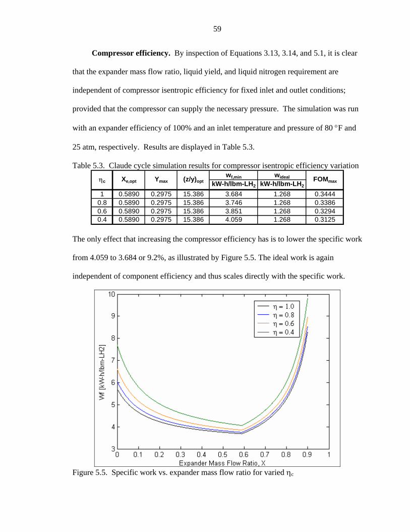
59

Compressor efficiency. By inspection of Equations 3.13, 3.14, and 5.1, it is clear

that the expander mass flow ratio, liquid yield, and liquid nitrogen requirement are

independent of compressor isentropic efficiency for fixed inlet and outlet conditions;

provided that the compressor can supply the necessary pressure. The simulation was run

with an expander efficiency of 100% and an inlet temperature and pressure of 80 °F and

25 atm, respectively. Results are displayed in Table 5.3.

Table 5.3. Claude cycle simulation results for compressor isentropic efficiency variation wf,min wideal

kW-h/lbm-LH2 kW-h/lbm-LH2

1 0.5890 0.2975 15.386 3.684 1.268 0.34440.8 0.5890 0.2975 15.386 3.746 1.268 0.33860.6 0.5890 0.2975 15.386 3.851 1.268 0.32940.4 0.5890 0.2975 15.386 4.059 1.268 0.3125

ηc Xe,opt Ymax (z/y)opt FOMmax

The only effect that increasing the compressor efficiency has is to lower the specific work

from 4.059 to 3.684 or 9.2%, as illustrated by Figure 5.5. The ideal work is again

independent of component efficiency and thus scales directly with the specific work.

Figure 5.5. Specific work vs. expander mass flow ratio for varied ηc

60

Comparing the figures of merit for the two cases in Figure 5.6 indicates a more

profound impact of the compressor efficiency on the cycle performance. A 60% decrease

in efficiency from ideal results in a 9.2% reduction in the FOM for the compressor case

compared to 7.8% for the expander. A greater emphasis should therefore be placed on

the development of high efficiency hydrogen compressors to minimize liquefaction

energy.

0.31

0.315

0.32

0.325

0.33

0.335

0.34

0.345

0.35

0.4 0.5 0.6 0.7 0.8 0.9 1Isentropic Efficiency

Figu

re o

f Mer

it (F

OM

)

Expander Efficiency Effect Compressor Efficiency Effect

Figure 5.6. Impact of compressor and expander efficiencies on Claude cycle FOM

Compressor inlet pressure. Compressor inlet pressure is varied to determine the

advantage of using pressurized electrolysis. A simulation was run for an outlet pressure

of 40 atm and compressor and expander efficiencies of 75 and 85%, respectively.

Table 5.4. Claude cycle simulation results for compressor inlet pressure variation P1 wf,min wideal

atm kW-h/lbm-LH2 kW-h/lbm-LH2

1 0.6230 0.2733 15.457 6.275 1.772 0.28245 0.6230 0.2733 15.457 5.050 1.521 0.3012

10 0.6230 0.2733 15.457 4.521 1.413 0.312515 0.6230 0.2733 15.457 4.210 1.349 0.320420 0.6230 0.2733 15.457 3.989 1.304 0.326825 0.6230 0.2733 15.457 3.817 1.268 0.3357

FOMmaxXe,opt Ymax (z/y)opt

61

Table 5.4 shows that the optimum expander mass flow ratio, maximum liquid yield, and

minimum liquid nitrogen requirement are independent of the compressor inlet pressure.

This is true because the inlet temperature and exit pressure are held constant and the

compression process is modeled as isothermal. Furthermore, the liquid yield and

expander mass flow ratio are decoupled from the compressor inlet and exit temperatures

by the 100% effective cooling bath assumption. The functional relationship between the

specific work and inlet pressure is graphically described in Figure 5.7.

3

3.5

4

4.5

5

5.5

6

6.5

0 5 10 15 20 25 30

Compressor Inlet Pressure (atm)

Wor

k pe

r Uni

t Mas

s LH

2

Figure 5.7. Effect of compressor inlet pressure on the specific work

Increasing the pressure from 1 to 25 atmospheres reduces the specific work requirement

by 39.2% while also reducing the theoretical work requirement by 28.4%; the net result is

an 18.9% increase in the figure of merit.

Compressor inlet temperature. Compressor inlet temperatures ranging from 0

to 80 °F are analyzed to gauge the merits for hydrogen pre-cooling using the combined

cycle. A simulation was run for an inlet pressure of 25 atm, exit pressure of 40 atm, and

compressor and expander efficiencies of 75 and 85%, respectively.

62

Results of the simulation are summarized in Table 5.5. An interesting result of

this simulation is the reduction in the figure of merit with lower inlet temperatures.

Table 5.5. Claude cycle simulation results for compressor inlet temperature variation T1 wf,min wideal

(F) kW-h/lbm-LH2 kW-h/lbm-LH2

0 0.6230 0.2733 15.621 3.802 1.004 0.263920 0.6230 0.2733 15.577 3.806 1.069 0.280840 0.6230 0.2733 15.535 3.809 1.134 0.297860 0.6230 0.2733 15.495 3.813 1.201 0.315080 0.6230 0.2733 15.457 3.817 1.268 0.3323

Ymax (z/y)opt FOMmaxXe,opt

This phenomenon is explained by the increase in the liquid nitrogen requirement due to

the assumption that Tc = T2. Reducing the inlet temperature of the compressor effectively

decreases Tc and lowers the enthalpy at state C. From Equation 3.14, the denominator hc

– ha is reduced from 187.2 Btu/lbm (435.5 kJ/kg) to 167.3 (Btu/lbm) 389.2 kJ/kg, thereby

increasing the liquid nitrogen requirement from 15.457 to 15.621 lbm-LN2/lbm-LH2.

This effect partially offsets the benefit of pre-cooling the hydrogen gas resulting in a

0.393% decrease in specific work. The ideal specific work simultaneously decreases by

20.8%. As a result, the FOM actually decreases by 20.6% from 80 to 0 °F. The liquid

nitrogen requirement and specific work in relation to the compressor inlet temperature is

presented in Figures 5.8 and 5.9.

15.4415.4615.4815.515.5215.5415.5615.5815.615.6215.64

01020304050607080

Compressor Inlet Temperature (F)

Liqu

id N

itrog

en R

equi

rem

ent

(lbm

/lbm

-LH

2)

Figure 5.8. Liquid nitrogen requirement vs. compressor inlet temperature

63

Figure 5.9 concludes that the reduction in specific liquefaction energy due to

decreased inlet temperature can be neglected within the specified range. A qualitative

comparison of the figures of merit made between cases three and four show that

increasing inlet pressure is significantly more effective in reducing the specific

liquefaction energy (Figure 5.10).

3.83.8023.8043.8063.8083.813.8123.8143.8163.8183.82

01020304050607080

Compressor Inlet Temperature (F)

Wor

k pe

r Uni

t Mas

s LH

2 (B

tu/lb

m)

Figure 5.9. Specific work requirement vs. compressor inlet temperature

The analysis concludes that the optimum operating point for the Claude cycle under

the assumed component efficiencies (ηe = 0.85, ηc = 0.75) is P1 = 25 atm. The cycle

parameter values are displayed in Table 5.6 at the optimum design point and at normal

operating conditions. The specific work of liquefaction is reduced by 46.7% and the

figure of merit is increased 18.9%.

The total energy required to produce and liquefy hydrogen is 28.656 kW-h/lbm-H2

(63.175 kW-h/kg-H2). Over 86% of this energy is consumed in electrolysis. Properties

at each state point are given for the optimum design condition in Appendix B. Given the

conclusion that compressor inlet temperature has little effect on the specific work, the

64

maximum hydrogen production rate of the combined cycle is 0.1775 lbm/hr or 7.21

gallons/day.

0.25

0.26

0.27

0.28

0.29

0.3

0.31

0.32

0.33

0.34Fi

gure

of M

erit

(FO

M)

Increasing Inlet Pressure Decreasing Inlet Temperature

Figure 5.10. Comparison of inlet pressure and temperature affect on the cycle FOM

Table 5.6. Claude cycle performance parameters for normal and optimum configuration Normal Optimum

T1 = 80F P1 = 1 atm T1 = 80F P1 = 25 atm

Xe,opt 0.6230 0.6230Ymax 0.2733 0.2733(z/y)opt 15.457 15.457wf,min

Btu/lbm-LH2 21411.70 13025.04kW-h/lbm-LH2 6.275 3.817

wideal

Btu/lbm-LH2 6046.88 4327.92kW-h/lbm-LH2 1.772 1.268

FOMmax 0.2824 0.3357

Ammonia-water Combined Cycle

The ammonia-water combined cycle was analyzed for a fixed power output to

observe the impact of expander efficiency on the heat and work requirements as well as

the cooling capacity. The simulation was run under the assumptions listed in chapter 3

while varying the expander isentropic efficiency from 10 to 100% in 10% increments.

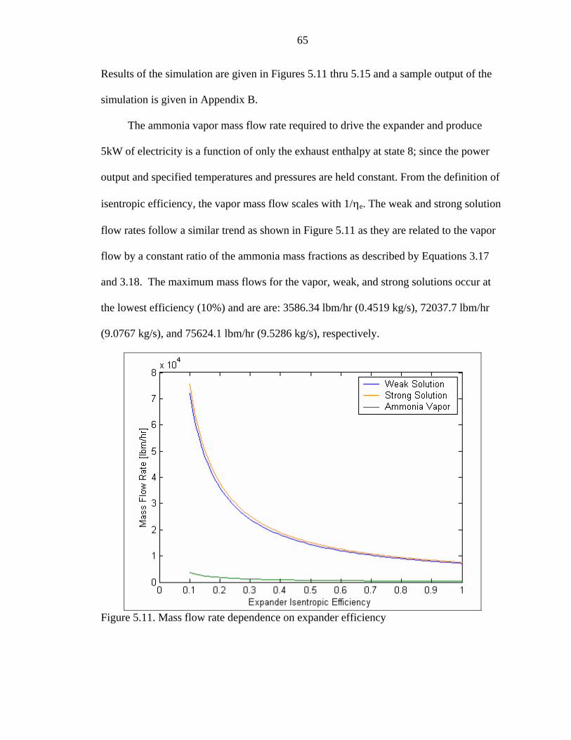
65

Results of the simulation are given in Figures 5.11 thru 5.15 and a sample output of the

simulation is given in Appendix B.

The ammonia vapor mass flow rate required to drive the expander and produce

5kW of electricity is a function of only the exhaust enthalpy at state 8; since the power

output and specified temperatures and pressures are held constant. From the definition of

isentropic efficiency, the vapor mass flow scales with 1/ηe. The weak and strong solution

flow rates follow a similar trend as shown in Figure 5.11 as they are related to the vapor

flow by a constant ratio of the ammonia mass fractions as described by Equations 3.17

and 3.18. The maximum mass flows for the vapor, weak, and strong solutions occur at

the lowest efficiency (10%) and are are: 3586.34 lbm/hr (0.4519 kg/s), 72037.7 lbm/hr

(9.0767 kg/s), and 75624.1 lbm/hr (9.5286 kg/s), respectively.

Figure 5.11. Mass flow rate dependence on expander efficiency

66

Likewise the minimum mass flows are (in the same order): 358.63 lbm/hr (0.0452

kg/s), 7203.77 (0.9077 kg/s), and 7562.41 (0.9529 kg/s). The mass fraction of the strong,

weak, and vapor streams are xS = 0.3988, xW = 0.3689, and xV = 1.0 (assumed). A

decrease in mass flow through the system manifests itself in the reduction of work and

heat interactions of the cycle for a given output as seen in Figures 5.12 and 13.

Figure 5.12. Pump work variation with expander efficiency

Minimum pump work, boiler heat input and absorber heat rejection are: 0.724 Hp

(0.540 kW), 331,566 Btu/hr (97.18 kW), and 321,117 Btu/hr (94.11 kW). The ideal

cooling capacity under these conditions is 9130.26 Btu/hr (2.68 kW). Figure 5.14

concludes that at least 60% efficient expansion is required to obtain any cooling capacity.

Below this point, the exhaust temperature of the expander exceeds the assumed

temperature of the substance to be cooled (85 °F). This effect is also evidenced in the

plot of the expander isentropic efficiency versus the cycle thermal efficiency (Figure

5.15).

67

Figure 5.13. Boiler heat input and absorber heat rejection vs. expander efficiency

Figure 5.14. Cycle cooling capacity as a function of expander efficiency

Thermal efficiency increases linearly with expander efficiency; however, a sudden

increase in slope occurs at approximately ηe = 0.6 at which point the cooling effect

68

begins to enhance the thermal efficiency of the cycle. The highest achievable thermal

efficiency for the given operating conditions is 7.22%.

Figure 5.15. Cycle thermal efficiency vs expander efficiency

The mass fraction of ammonia entering the expander was analyzed more closely to

judge the assumption of pure vapor leaving the rectifier and to determine the impact that

trace quantities of water have on the cycle performance. The analysis was carried out for

an ideal expander. Figure 5.16 shows the profound negative effect on cooling capacity.

The cooling capacity diminishes to zero rapidly as trace amounts of water are introduced

into the expander stream up to only 2.5% by mass. Boiler heat input is reduced from

331,566 Btu/hr (97.18 kW) to 320,934 Btu/hr (94.06); however, thermal efficiency is

reduced 9.26% from 7.22% to 6.55% because of the lost cooling benefit. Another

concern is that the expander exhaust temperature drops below the mixture dew point as

shown in Figure 5.17. At a 2.5% water vapor concentration by mass, the mixture quality

is 0.967. This most likely is not an issue for compliant devices such as scrolls in which a

69

small quantity of liquid can be tolerated, or with high-speed devices such as turbines, in

which the residence time of the fluid is shorter than the time required for condensation to

occur (metastable condition).

010002000300040005000600070008000900010000

0.9750.980.9850.990.9951

Expander Ammonia Mass Fraction, x7

Coo

ling

Cap

acity

(btu

/hr)

Figure 5.16. Effect of trace amounts of water within in the expander inlet stream on

cycle cooling capacity

250260270280290300310320330

0.9750.980.9850.990.9951

Expander Ammonia Mass Fraction, x7

Tem

pera

ture

(K)

Isentropic Exhaust Dew Point at 40 psia

Figure 5.17. Expander exhaust and dew point temperature at several water concentrations

These results show that rectifier design is a crucial element for the success of a small-

scale combined cycle in the hydrogen production field in which high efficiency translates

into greater liquid yield per unit energy input.

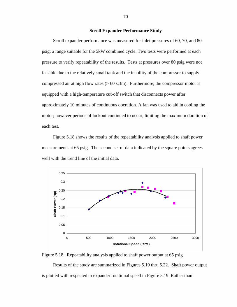
70

Scroll Expander Performance Study

Scroll expander performance was measured for inlet pressures of 60, 70, and 80

psig; a range suitable for the 5kW combined cycle. Two tests were performed at each

pressure to verify repeatability of the results. Tests at pressures over 80 psig were not

feasible due to the relatively small tank and the inability of the compressor to supply

compressed air at high flow rates (> 60 scfm). Furthermore, the compressor motor is

equipped with a high-temperature cut-off switch that disconnects power after

approximately 10 minutes of continuous operation. A fan was used to aid in cooling the

motor; however periods of lockout continued to occur, limiting the maximum duration of

each test.

Figure 5.18 shows the results of the repeatability analysis applied to shaft power

measurements at 65 psig. The second set of data indicated by the square points agrees

well with the trend line of the initial data.

0

0.05

0.1

0.15

0.2

0.25

0.3

0.35

0 500 1000 1500 2000 2500 3000

Rotational Speed (RPM)

Shaf

t Pow

er (H

p)

Figure 5.18. Repeatability analysis applied to shaft power output at 65 psig

Results of the study are summarized in Figures 5.19 thru 5.22. Shaft power output

is plotted with respected to expander rotational speed in Figure 5.19. Rather than

71

beginning at a maximum value and decreasing monotonically with RPM as expected, the

power output reaches a maximum at approximately 1500 RPM before decreasing toward

zero in all three cases. This is thought to occur due to choked conditions at the expander

exit. Flow becomes choked when the port to fitting area ratio is smaller than the critical

area ratio given by the temperature and pressure of the exiting air. The area of the

expander exit port and fitting is 0.375” and 0.25”, respectively. Further evidence of

choked flow is given by the fact that the maximum attainable rotational speed is only

3000 RPM at source pressures up to 110 psig, whereas the TRS-90 scroll compressor can

normally achieve speeds of up to 9000 RPM (Sanden engineer, personal conversation).

0

0.05

0.1

0.15

0.2

0.25

0.3

0.35

0.4

0 500 1000 1500 2000 2500 3000

Rotational Speed (RPM)

Shaf

t Pow

er (H

p)

60 psi 70 psi 80 psi

Figure 5.19. Shaft power vs. rotational speed at 60, 70, and 80 psig inlet pressure

A similar trend is witnessed with isentropic efficiency, ηe (Figure 5.20). Low

values of ηe are attributed to the poor volumetric efficiency, ηv, of the expander at low

RPM and relatively high torsional load. Increased torsional resistance raises the pressure

within each pocket of the scroll, enhancing tip leakage and reducing volumetric

efficiency. Figure 5.21 illustrates the relationship between volumetric efficiency and

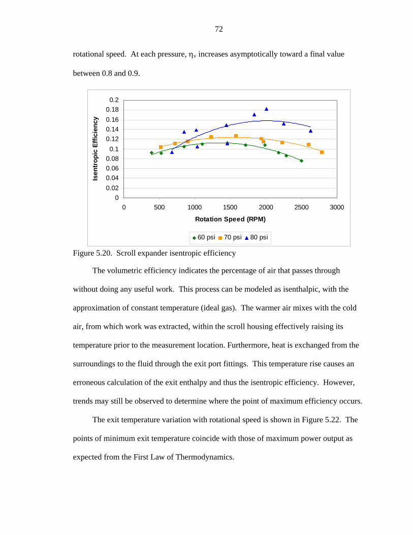
72

rotational speed. At each pressure, ηv increases asymptotically toward a final value

between 0.8 and 0.9.

00.020.040.060.080.1

0.120.140.160.180.2

0 500 1000 1500 2000 2500 3000

Rotation Speed (RPM)

Isen

trop

ic E

ffici

ency

60 psi 70 psi 80 psi

Figure 5.20. Scroll expander isentropic efficiency

The volumetric efficiency indicates the percentage of air that passes through

without doing any useful work. This process can be modeled as isenthalpic, with the

approximation of constant temperature (ideal gas). The warmer air mixes with the cold

air, from which work was extracted, within the scroll housing effectively raising its

temperature prior to the measurement location. Furthermore, heat is exchanged from the

surroundings to the fluid through the exit port fittings. This temperature rise causes an

erroneous calculation of the exit enthalpy and thus the isentropic efficiency. However,

trends may still be observed to determine where the point of maximum efficiency occurs.

The exit temperature variation with rotational speed is shown in Figure 5.22. The

points of minimum exit temperature coincide with those of maximum power output as

expected from the First Law of Thermodynamics.

73

0

0.1

0.2

0.3

0.4

0.5

0.6

0.7

0.8

0.9

0 500 1000 1500 2000 2500 3000 3500

Rotational Speed (RPM)

Volu

met

ric E

ffici

ency

60 psi 70 psi 80 psi

Figure 5.21. Volumetric efficiency variation with expander rotational speed

3032

34363840

424446

4850

0 500 1000 1500 2000 2500 3000

Rotational Speed (RPM)

Exit

tem

pera

ture

(F)

60 psi 70 psi 80psi

Figure 5.22. Expander exit temperature and rotational speed relationship

The maximum power output of 0.368 Hp (0.274 kW) occurred at 1460 RPM for the

80-psig inlet pressure case. The most efficient operating point is 18.2%. Rotational

speed, inlet pressure, and power output at this point is 2000, 80 psig, and 0.282 Hp. The

temperature of the working fluid (excluding leakage) is found at any point using the

volumetric efficiency and flow rate in Equation 5.5.

74

( )v

inletvexit

wf

inletleakageexitwf

TTcfm

TcfmTT

ηη−−

=−

=1

(5.5)

Therefore, with a volumetric efficiency of 0.6092 and temperatures of 71.6 °F and 31.5

°F at the inlet and exit at this point, the temperature of the working fluid is 4.77 °F.

The low value of isentropic efficiency is due primarily to leakage caused by the

density mismatch. The TRS-90 is designed for R-134A with a density of 0.262 lbm/ft3 at

STP whereas the density of air at STP is .07298 lbm/ft3; nearly 3.6 times lower than R-

134A, and the density of ammonia is 0.04333 lbm/ft3; 1.6 times lower than air. The

performance of the expander with ammonia is expected to be worse than with air because

higher pressures are required for a unit volume of ammonia to store an equal amount of

energy as a unit volume of air at a given temperature. This relationship is arrived at by

considering the ideal gas law as a first approximation (Equation 5.6).

86.1≅=⇒=air

ammonia

ammonia

air

airammonia mm

pp

mTp

mTp (5.6)

Higher pressures lead to increased leakage within the scroll and a loss of performance.

Additionally, ammonia is a smaller molecule than air and much smaller than R-134A,

further facilitating tip leakage and reducing efficiency.

Fundamental design changes are required for the scroll concept to be utilized as

an expander. The geometry of each scroll element should be altered such that the total

number of chambers is increased as shown in Figure 5.23. This design reduces pressure

differences between chambers and hence leakage (Hans-Joachim and Radermacher,

2003).

75

Figure 5.23. Comparison of optimum geometries of a scroll compressor (left) and

expander (right) (Adapted from Hans-Joachim and Radermacher, 2003)

76

CHAPTER 6 RECOMMENDATIONS

Analytical Study

The analytical study of the electrolyzer, Claude cycle, and ammonia-based

combined power/cooling cycle examined a limited range of operating parameters. By

modeling the overall process with a program such as ASPEN, a greater number of

operating configurations could be analyzed.

ASPEN is a chemical processing software package that allows the user design a

cycle and specify a set or range of operating and boundary conditions. Using algorithms

included in the code for most devices, ASPEN performs a complete thermodynamic

analysis and outputs user specified data in an interactive manner.

Additionally, an optimization of the combined cycle for maximum hydrogen

production would indicate the operating conditions, power output, and overall system

size required to minimize energy cost. The economic viability of a large-scale

implementation of this system should be examined through a life-cycle cost analysis.

Scroll Expander Performance Test

The scroll expander used in the performance test was an automotive air-

conditioning compressor modified to run in reverse. Recommendations for future scroll

expander experimentation are:

13. Test the expander in a closed loop system with ammonia vapor 14. Pre-heat the inlet vapor to simulated the combined cycle operating conditions 15. Re-design the compressor housing to allow higher flow rates and eliminate choking 16. Design an oil injection and separation system to reduce leakage losses 17. Use a dynometer or motor to improve control on the applied torque

77

Future work should also include improvements to the scroll design. Manufacturing

the scroll involute using the optimum expander geometry shown in Figure 5.23 would

improve its performance as an expander. Furthermore, the use of low-friction materials

such as those under development at the University of Florida would eliminate the need

for an oiling system, making the scroll an attractive design for the ammonia based

combined power/cooling cycle.

78

CHAPTER 7 CONCLUSIONS

Global energy consumption is projected to increase 54% over the next 25 years.

With proven oil reserves being called into question beyond 2030 it is important to

develop renewable technologies to sustain the future global energy demand. By

introducing an alternative fuel for transportation only, oil consumption can be reduced by

as much as 20%.

Hydrogen has many characteristics that make it a desirable fuel. It has the highest

energy content per unit mass of any known fuel – nearly 3 times higher than gasoline, it

burns cleanly and efficiently, and it can be produced from water via electrolysis powered

by renewable energy. Two major obstacles to the emergence of a hydrogen economy are

the limited means available to efficiency produce mass quantities of hydrogen from

renewable energy sources and the storage issues related to the low energy density of

hydrogen. Liquefying hydrogen provides a solution to its low density; however, the

process requires additional energy.

This thesis explored the possibility of using a 5-kW ammonia-based combined

power/cooling cycle to produce hydrogen from renewable resources and pre-cool it prior

to liquefaction in an effort to reduce the overall energy consumption. The advantage of

this cycle is its ability to utilize low temperature heat sources available from solar and

geothermal resources.

Simulations of the Claude liquefaction process and the 5-kW ammonia-based

combined power/cooling cycle were developed to model the effects of component

79

efficiencies and operating parameters on the maximum hydrogen production rate and

system energy requirement. Additionally, a performance test of a scroll compressor was

performed to gauge its effectiveness as an expander for the combined cycle.

Conclusions resulting from tests and analyses are summarized below:

1. Pre-cooling hydrogen has little effect on the specific liquefaction energy and is

detrimental to the liquefier efficiency.

2. Pressurized electrolysis is the most effective method of reducing the energy

consumed in liquefaction.

3. The total energy required to produce and liquefy hydrogen is 28.656 kW-h/lbm-H2

(63.175 kW-h/kg-H2); 86% of which is consumed during electrolysis. A maximum of

7.21 gallons (27.3 liters) per day of liquid hydrogen can be produced from a 5-kW

combined cycle.

4. The mass flows as well as the heat and work interactions of the 5-kW combined cycle

scale with inverse of expander efficiency (1/ηe). Sixty percent expansion efficiency

is required to extract cooling from the cycle.

5. Cooling capacity of the cycle is extremely sensitive to the vapor mass fraction of the

expander inlet stream. At 2.5% water by mass and for perfect expansion, the cooling

capacity completely diminishes.

6. Results of the performance test indicate that scroll compressors operate poorly as

expanders. Low isentropic efficiencies result from leakage around the scroll tips.

Improvements in the scroll design such as increasing the wrap of each scroll element

and using low-friction material for oil-less operation would make the scroll an

efficient expansion device suitable for the combined cycle.

80

APPENDIX A COMPUTER PROGRAM FOR CYCLE SIMULATIONS

Two computer programs were written to assist in the evaluation of thermodynamic

properties and to perform cycle analyses of the Claude liquefaction cycle and the

ammonia-water combined power/cooling cycle. A description of each program is given

below, including portions of the source code.

Claude Cycle Simulation

The program was written to assist in the parametric analysis of the specific work

and efficiency of the Claude cycle. A subroutine was included to evaluate the

thermodynamic properties at each state point coinciding with Figure 2.6. The code has

the flexibility of single point calculations or variable inputs for a parametric analysis.

Thermodynamic Property Evaluation

The property code incorporates portions of RGAS and PSAT, two programs written

by Dr. Roger Gater (2001). Property evaluation is carried out as a subroutine of the

overall cycle simulation. The properties defined by user input and the listed assumptions

are passed into either routine depending on the fluid condition. For saturated conditions,

the pressure is defined; for superheated vapor, pressure-temperature, pressure-enthalpy,

or pressure-entropy is input. Properties are then evaluated using the Redlich-Kwong gas

model and returned to the main program. Critical properties and coefficients required by

the Redlich-Kwong model are listed in Table A.1.

81

Program Description

The Claude cycle simulation program is written in MatLAB. It consists of three

sub-routines and a data file: saturation2.m, gas_properties.m, gas_properties_base.m,

gas.dat, all of which must be present for the program to operate. The program begins by

reading data from the “gas.dat” file. It then asks for user input of compressor inlet

temperature and pressure; giving the option of English or SI units. From the user input

and given assumptions, the thermodynamic properties at each state point are evaluated by

the “gas_properties.m” subroutine. If saturated conditions are known to exist,

“saturation2.m is invoked. The key performance parameters of the Claude cycle are then

calculated using the equations of Chapter 3. Results are output to the screen in figure

form. Additional aspects of the program are described by the imbedded comments.

Main Program - Claude.m

[gas_num gas_name R Tc Pc cpoR a b c Zc A w] = textread('GAS.dat','%f %s %f %f %f %f %f %f %f %f %f %f', 'headerlines',1); units = input('Select Units: 0 = Metric, 1 = English: '); while (units < 0) | (units > 1) units = input('\nError, Try again: '); end if units == 0 T1 = input('\nEnter compressor inlet temperature (K): '); P1 = input('\nEnter compressor inlet pressure (atm): '); P1 = P1 * 1.0132; else T1 = input('\nEnter compressor inlet temperature (F): '); T1 = (T1 - 32)*5/9 + 273.15; P1 = input('\nEnter compressor inlet pressure (atm): '); P1 = P1 * 1.0132; end P2 = input('\nEnter compressor discharge pressure (atm): '); P2 = P2 * 1.0132; eta_e = input('\nEnter expander adiabatic efficiency: '); %eta_e = .85; eta_c = input('\nEnter compressor efficiency: '); %eta_c = .75; % properties in J/g or kJ/kg P_stp = 1.0132; %bar gas = 10; % selects hydrogen gas from GAS.DAT data file Pe = P_stp; Pg = P_stp; Pf = P_stp; P7 = P_stp; P8 = P_stp;

82

P9 = P_stp; P10 = P_stp; P10a = P_stp; PA = P_stp; PC = P_stp; P2b = P2; P3 = P2; P4 = P2; P5 = P2; HC1 = 175.1; HC2 = 312.97; %Heats of conversion kJ/kg WN2 = 1783.623; %kJ/kg-N2 Energy of LN2 liquefaction T2 = T1; T10 = T1; TC = T1; %State g and f %call saturation program routine = 1; Ps = Pg; P = Pg; [Ts,Zf,Zg,vf,vg,hfg,ufg,sfg] = saturation2(Ps,R(gas),Tc(gas),Pc(gas),Zc(gas),A(gas),w(gas)); Tg = Ts; Tf = Ts; T = Ts; gas_properties; hg = h; sg = s; hf = hg - hfg; sf = sg - sfg; %State 1 routine = 1; %pressure and temp specified T = T1; P = P1; gas_properties; h1 = h; s1 = s; %State 2 routine = 1; %isothermal compression T = T2; P = P2; gas_properties; h2 = h; s2 = s; %State 2b Ps = P_stp; gas = 13; %sets nitrogen properties Ts = saturation2(Ps,R(gas),Tc(gas),Pc(gas),Zc(gas),A(gas),w(gas)); %calculates temperature of nitrogen gas = 10; %returns to hydrogen T2b = Ts; T = T2b; P = P2b; routine = 1; gas_properties; h2b = h; s2b = s; %State 3 T3 = T2b; test = 0; while T3 >= 70 % above critical temperature of hydrogen (asymptotic problems) routine = 1; T = T3; P = P3; gas_properties; h3 = h; s3 = s; %state e_s routine = 2; %test to see if saturated conditions exist P = Pe; Ps = Pe; se = s3; ss = se; gas_properties; he_s = h; Te_s = T; if Te_s <= Tf xe = (se - sf)/(sfg);

83

he_s = hf + xe*(hfg); Te_s = Tf; %isentropic temperature end if (h3 - he_s) > test T3opt = T3; Te_s_opt = Te_s; delta_h_opt = h3 - he_s; h3opt = h3; s3opt = s3; he_sopt = he_s; end test = h3 - he_s; T3 = T3 - .1; end %state e routine = 3; % pressure and enthalpy specified he = h3opt - eta_e*(delta_h_opt); hh = he; P = Pe; gas_properties; Te = T; se = s; %state 4 routine = 1; T = Te; P = P1; T4 = Te; gas_properties; h4 = h; s4 = s; %state 7 and 8 routine = 1; T = Te; P = Pe; T7 = Te; T8 = Te; gas_properties; h7 = h; h8 = h; s7 = s; s8 = s; %state 10 routine = 1; T = T10; P = P10; gas_properties; h10 = h; s10 = s; %state 10a routine = 1; T = T2b; P = P10; gas_properties; h10a = h; s10a = s; %state A (saturated liquid) routine = 1; Ps = PA; P = PA; gas = 13; [Ts,Zf,Zg,vf,vg,hfg,ufg,sfg] = saturation2(Ps,R(gas),Tc(gas),Pc(gas),Zc(gas),A(gas),w(gas)); TA = Ts; gas_properties; hgA = h; sgA = s; hA = hgA - hfg; sA = sgA - sfg;

84

%state C routine = 1; T = TC; P = PC; gas_properties; hC = h; sC = s; gas = 10; %return to hydrogen %Specific work, liquid yield, liquid nitrogen requirement, and figure of merit calculation X(1) = 0; step = .001 for i = 1:1/step X(i+1) = X(i) + step; y(i) = ((h10a-h2b) + eta_e*X(i)*(delta_h_opt))/(h10a - hf + HC2); if y(i) >= .725*(1 - X(i)) %.725 found from iterative procedure on HX 3 y(i) = .725*(1-X(i)); end z(i) = (HC1 + (h2 - h10) + eta_e*X(i)*(delta_h_opt) + y(i)*(h10 - hf + HC2))/(hC - hA); if units == 0 W(i) = (((h2 - h1) - T1*(s2 - s1))/eta_c - eta_e*X(i)*(delta_h_opt))/3600; %work per unit mass compressed Wf(i) = W(i)/y(i) + z(i)/y(i)*WN2/3600; %work per unit mass liquefied kJ/kg W_ideal = ((hf - h1) - T1*(sf - s1))/3600; else W(i) = (((h2 - h1) - T1*(s2 - s1))/eta_c - eta_e*X(i)*(delta_h_opt))/(2.326*3412); Wf(i) = W(i)/y(i) + z(i)/y(i)*WN2/(2.236*3412); W_ideal = ((hf - h1) - T1*(sf - s1))/(2.326*3412); end FOM(i) = W_ideal/Wf(i); if X(i+1) >= .9 break end end z(i+1) = z(i); Wf(i+1) = Wf(i); W(i+1) = W(i); FOM(i+1) = FOM(i); y(i+1) = y(i); Xopt = (1 - max(y)/.725) Ymax = max(y) Wfopt = min(Wf) FOMopt = max(FOM) zopt = min(z./y) W_ideal figure(1) plot(X,Wf) title('Work Per Unit Mass LH2 vs. Expander Mass Flow Ratio, X'); xlabel('Expander Mass Flow Ratio, X') ylabel('Wf [kW-h/lbm-LH2]')

85

Saturation Property Evaluation - Saturation2.m

function [Ts,Zf,Zg,vf,vg,hfg,ufg,sfg] = saturation2(Ps,R,Tc,Pc,Zc,A,w) Psr = Ps/Pc; Tsr = (A + w*log(Psr))/(A - log(Psr)); Ts = Tsr*Tc; Zfg = .824*(log(1.3/(Psr + .3)))^.467; Zf = Zc*Psr*( 1 - Tsr^1.72*(1/Tsr - 1)^.295); Zg = Zfg + Zf; vf = Zf*R*Ts/Ps; vg = Zg*R*Ts/Ps; hfg = R*Tc*Zfg*(A*Tsr^2*(1 + w) / (Tsr + w)^2); ufg = hfg - Ps*(vg - vf); sfg = hfg/Ts; %need to add warning about pressure and temperature above critical point Gas Thermodynamic Property Evaluation – Gas_properties.m

%P & T given cpo = R(gas)*cpoR(gas); T0 = 300; P0 = 1; if routine == 1 [v,u,h,s] = gas_properties_base(T,P,R(gas),cpo,Tc(gas),Pc(gas),a(gas),b(gas),c(gas)); end if routine == 2 T = 1.2 * T0*exp(.8*ss/cpo + (R(gas)/cpo)*log(P/P0)); errorS = 1; while errorS > 1E-6 [v,u,h,s] = gas_properties_base(T,P,R(gas),cpo,Tc(gas),Pc(gas),a(gas),b(gas),c(gas)); errorS = abs(s - ss)/(abs(s+ss)+1); T = T*(.8 + .2*exp((ss - s)/cpo)); Tr = T/Tc; end end if routine == 3 T = 1.2*T0 + hh/cpo; errorH = 1; while errorH > 1E-6 [v,u,h,s] = gas_properties_base(T,P,R(gas),cpo,Tc(gas),Pc(gas),a(gas),b(gas),c(gas)); errorH = abs(h - hh)/(abs(h + hh)+100); T = T + .5*(hh-h)/cpo; Tr = T/Tc; end end Gas properties base.m

function [v,u,h,s] = gas_properties_base(T,P,R,cpo,Tc,Pc,a,b,c) alpha = .42748; beta=.08664; T0 = 300; P0 = 1;

86

Zp = 1; errorZ = 1; Tr = T/Tc; Pr = P/Pc; tau = (T/T0) - 1; while errorZ > 1E-6 vr = Zp*Tr/Pr; Z = 1 + beta/(vr - beta) - alpha/((vr + beta)*Tr^1.5); errorZ = abs(Z - Zp)/(Z + Zp); Zp = .8*Zp + .2*Z; end v = Z*R*T/P; vr = Z*Tr/Pr; phi = 1.25*vr^.1; ud = R*Tc*phi*1.5*(alpha/beta)/Tr^.5*log((vr + beta)/vr); hd = ud + (1 - Z)*R*T; sd = R*(ud/(R*Tc*Tr) + log(vr/(vr - beta)) - (alpha/beta)/Tr^1.5*log((vr + beta)/vr) - log(Z)); hig = cpo*T0*(tau + a*tau^2/2 + b*tau^3/3 + c*tau^4/4); uig = hig - R*T; sig0 = cpo * ((1 - a + b - c)*log(tau + 1) + (a - b + c)*tau + (b - c)*tau^2/2 + c*tau^3/3); sig = sig0 - R*log(P/P0); u = uig - ud; h = hig - hd; s = sig - sd;

Table A.1. Critical properties and coefficients contained within the “gas.dat” file Hydrogen Nitrogen

R 4.124 0.2968Tc 33.3 126.2Pc 13 33.9

Cpo/R 3.47 3.503a 2.49E-02 2.98E-03b -6.75E-03 3.50E-02c 2.00E-03 -5.86E-03

Zc 0.36 0.291A 4.925 5.64w 0.1415 0.0039

Ammonia-Based Combined Power/Cooling Cycle Simulation

The program was written to assist in the parametric analysis of the energy transfer

and cooling capacity dependence of the combined cycle on expander isentropic efficiency

and ammonia vapor mass fraction.

87

Thermodynamic Property Evaluation

Thermodynamic properties of the ammonia-water mixture and pure ammonia vapor

are evaluated using subroutines adapted from a program developed by Tamm (2003). The

evaluation method is based on a Gibbs free energy approach incorporating experimental

correlations. A detailed description of the evaluation method and the coefficients used

for the calculations are outlined by Tamm (2003).

Program Description

The combined cycle simulation program consists of a main program written in

MatLAB, “combined cycle.m” and five property evaluation subroutines:

ammonia_water.m, PTX.m, bubble_dew.m, critical_properties.m, and hsv_properties.m.

The main program accepts user input values of cycle high and low pressure as well as the

absorber and boiler temperatures. Each state point corresponding to Figure 2.7 is defined

from these inputs and by the assumptions listed in Chapter 3. The program evaluates the

thermodynamic properties at each point and uses these values to calculate the mass flows,

mass fractions, energy transfers, and efficiencies given by Equations 3.16 thru 3.25.

Results are output to text file named results.txt and displayed in several graphs. A

sample output of the program is given in Appendix B. Additional aspects of the program

are described by the imbedded comments.

Combined Cycle Main Program – Combined_cycle.m

%This program calculates the state points, work and heat exchanges, and flow rates %of the combined cycle for varied turbine isentropic efficiencies using the user %inputs of high pressure,low pressure, boiler temperature, and absorber temperature. %The turbine isentropic efficiency is varied from 10 to 100% to study its effect on %the overall cycle efficiency. % %Results are output to results.txt and graphs % %This program can easily be adapted for different operating conditions by %adjusting values in the assumptions section. %

88

%Sub-programs necessary for operation: ammonia_water.m, PTx.m, hsv_properties.m, %critical_props.m, bubble_dew.m, bubble_dew_base.m clear all; clc; cycle = 1; %signifies whether inputs are for cycle or individual states fprintf('\n***********************************************\n'); fprintf('* Combined Cycle Analysis *\n'); fprintf('* Analysis code written by Robert Reed *\n'); fprintf('* Property code written in C++ by Gunner Tamm *\n'); fprintf('* Adapted to MatLAB by Robert Reed *\n'); fprintf('* September 12, 2004 *\n'); fprintf('***********************************************\n'); fprintf('IMPORTANT: This program consists of six sub-routines which must be present:\n'); fprintf('\tammonia_water.m, bubble_dew_base.m, bubble_dew.m, critical_props.m,\n\thsv_properties.m, and PTx.m\n\n'); P_low = input('Enter the cycle low pressure (psia): '); P_low = P_low/14.504; P_high = input('Enter the cycle high pressure (psia): '); P_high = P_high/14.504; while P_high <= P_low fprintf('High pressure must be greater than low pressure!!!\n'); P_high = input('Try again: '); P_high = P_high/14.504; end Tabs = input('Enter absorber temperature (F): '); Tabs = (Tabs - 32)/1.8 + 273.15; Tboil = input('Enter boiler temperature (F): '); Tboil = (Tboil - 32)/1.8 + 273.15; while Tboil <= Tabs fprintf('Boiler temperature must be greater than absorber temperature!!!\n'); Tboil = input('Try again: '); Tboil = (Tboil - 32)/1.8 + 273.15; end %Future additions will include cooling and heating hot water flow rates. % Tcws = input('Enter cooling water source temperature (F): '); % Tcwr = input('Enter cooling water return temperature (F): '); % Thws = input('Enter heating hot water source temperature (F): '); % Tcwr = input('Enter heating hot water source temperature (F): '); %assumptions x7 = 1; %pure ammonia vapor exiting the rectifier %x7 = input('\nEnter mass fraction ammonia entering turbine: '); Elec = 5; %Electrical output of the generator [kW]. etaG = .75; %Generator efficiency eps = .85; %recovery HE effectiveness WT = Elec/etaG; %Define all states by calling ammonia_water.m %state 1 P = P_low; T = Tabs; option = 8; %option sets the sub-routine used in ammonia_water.m ammonia_water; P1 = P; T1 = T; h1 = hL; s1 = sL; v1 = vL; x1 = xb; %return results %state 2 P = P_high; T2 = T1; x = x1; option = 1; ammonia_water; P2 = P; T2 = T; h2 = hm; s2 = sm; v2 = vm; x2 = x;

89

%state 4 P = P_high; T = Tboil; option = 8; ammonia_water; P4 = P; T4 = T; h4 = hL; s4 = sL; v4 = vL; x4 = xb; %could also have the actual vapor exit state %state 5 P = P_high; x = x4; option = 1; T = T4 - eps*(T4 - T2); %assuming equal specific heats ammonia_water; T5 = T; P5 = P; h5 = hm; s5 = sm; v5 = vm; x5 = x; %state 6 P = P_low; h = h5; x = x4; option = 3; ammonia_water; T6 = T; P6 = P; h6 = h; s6 = sm; v6 = vm; x6 = x; %state 9 T = 302.594444444; %assumed to be 85F for air/hydrogen cooling P = P_low; x = x7; option = 1; ammonia_water; T9 = T; P9 = P; h9 = hm; s9 = sm; v9 = vm; x9 = x; %state 7 P = P_high; T = Tboil; x = x7; option = 1; ammonia_water; P7 = P; T7 = T; h7 = hm; s7 = sm; v7 = vm; %state 8s Imaginary state obtained from isentropic expansion P = P_low; s = s7; x = x7; option = 4; ammonia_water; P8s = P; T8s = T; h8s = hm; s8s = s; v2s = v2; x8s = x; %state 8 etaT(1) = .1; %initial value of the turbine efficiency step = .01; %step change in loop of the turbine efficiency for n = 1:1/step P = P_low; x = x7; h = h7 - etaT(n)*(h7 - h8s); option = 3; ammonia_water; P8 = P8s; T8(n) = T; h8(n) = h; s8(n) = sm; v8(n) = vm; x8 = x; %Calculate solution mass flow rates mT(n) = WT / (h7 - h8(n)); %Turbine mass flow mS(n) = mT(n)*((x7 - x4)/(x1 - x4)); % Strong solution mass flow rate mW(n) = mS(n) - mT(n); %Weak solution mass flow rate %state 3 P = P_high; x = x1; option = 1; T = eps*mW(n)*(T4 - T2)/mS(n) + T2; %assuming equal specific heats ammonia_water; T3 = T; P3 = P; h3 = hm; s3 = sm; v3 = vm; x3 = x; %Heat and work flows

90

Qin(n) = mW(n)*h4 + mT(n)*h7 - mS(n)*h3; %heat input to vapor generator Qout(n) = mW(n)*h6 + mT(n)*h9 - mS(n)*h1; %heat rejected from absorber Qc(n) = mT(n)*(h9 - h8(n)); %Cooling capacity WP(n) = mS(n)*(h2-h1); %Pump work if Qc(n) < 0 % This step disallows negative cooling capacity Qc(n) = 0; end COP = 3; %typical value eta_cycle(n) = (WT - WP(n) + Qc(n)/COP) / Qin(n); %cycle efficiency etaT(n+1) = etaT(n) + step; %set new value for next loop end %Set vector lengths equal, last value is ignored Qin(n+1) = Qin(n); Qout(n+1) = Qout(n); WP(n+1) = WP(n); Qc(n+1) = Qc(n); eta_cycle(n+1) = eta_cycle(n); mS(n+1) = mS(n); mW(n+1) = mW(n); mT(n+1) = mT(n); results = fopen('results.txt','w'); fprintf(results,'***************************\n'); fprintf(results,'* Cycle Analysis Results *\t\t Created: %s\n',datestr(now)); fprintf(results,'***************************\n\n\n'); fprintf(results,'Assumptions:\t Saturated conditions at states 1 and 4.\n'); fprintf(results,' \t Component pressure losses are negligible.\n'); fprintf(results,' \t Equal weak and strong solution specific heats.\n'); fprintf(results,' \t Superheater temperature equal to boiler temperature.\n'); fprintf(results,' \t Mass fraction of ammonia in the rectifier exit stream, x7 = %g\n',x7); fprintf(results,' \t Evaporator exit temperature = %g F (%.2f C)\n',((T9-273.15)*1.8+32),T9-273.15); fprintf(results,' \t Electric generator efficiency = %g%%\n',etaG*100); fprintf(results,' \t Recovery heat exchanger effectiveness = %g\n',eps); fprintf(results,' \t Electric generator output = %g kW\n\n\n',Elec); fprintf(results,'User Inputs:\t Absorber temperature = %g F (%g C)\n',(Tabs-273.15)*1.8+32,Tabs-273.15); fprintf(results,' \t Boiler temperature = %g F (%g C)\n',(Tboil-273.15)*1.8+32,Tboil-273.15); fprintf(results,' \t System low pressure = %g psia (%g bar)\n',P_low*14.504,P_low); fprintf(results,' \t System high pressure = %g psia (%g bar)\n',P_high*14.504,P_high); fprintf(results,'______________________________________________________________________________________________________________\n\n'); fprintf(results,'\t State 1 \t\t\t\t\t\t State 2 \t\t\t\t\t\t State3\n\n'); fprintf(results,' T = %g F (%.2f C) \t\t\t\t T = %g F (%.2f C) \t\t\t\t T = %g F (%.2f C)\n',(T1-273.15)*1.8+32,T1-273.15,(T2-273.15)*1.8+32,T2-273.15,(T3-273.15)*1.8+32,T3-273.15); fprintf(results,' P = %g psia (%.2f bar) \t\t\t P = %g psia (%.2f bar) \t\t\t P = %g psia (%.2f bar)\n',P1*14.504,P1,P2*14.504,P2,P2*14.504,P2); fprintf(results,' h = %g BTU/lbm (%.2f kJ/kg) \t h = %g BTU/lbm (%.2f kJ/kg) \t h = %g BTU/lbm (%.2f kJ/kg)\n',h1/2.326,h1,h2/2.326,h2,h3/2.326,h3); fprintf(results,' s = %g BTU/lbm-R (%.4f kJ/kg-K) \t s = %g BTU/lbm-R (%.4f kJ/kg-K) \t s = %g BTU/lbm-R (%.4f kJ/kg-K)\n\n',s1/4.1868,s1,s2/4.1868,s2,s3/4.1868,s3); fprintf(results,'\t State 4 \t\t\t\t\t\t State 5 \t\t\t\t\t\t State6\n\n'); fprintf(results,' T = %g F (%.2f C) \t\t\t\t T = %g F (%.2f C) \t\t\t\t T = %g F (%.2f C)\n',(T4-273.15)*1.8+32,T4-273.15,(T5-273.15)*1.8+32,T5-273.15,(T6-273.15)*1.8+32,T6-273.15); fprintf(results,' P = %g psia (%.2f bar) \t\t\t P = %g psia (%.2f bar) \t\t\t P = %g psia (%.2f bar)\n',P4*14.504,P4,P5*14.504,P5,P6*14.504,P6); fprintf(results,' h = %g BTU/lbm (%.2f kJ/kg) \t h = %g BTU/lbm (%.2f kJ/kg) \t h = %g BTU/lbm (%.2f kJ/kg)\n',h4/2.326,h4,h5/2.326,h5,h6/2.326,h6); fprintf(results,' s = %g BTU/lbm-R (%.4f kJ/kg-K) \t s = %g BTU/lbm-R (%.4f kJ/kg-K) \t s = %g BTU/lbm-R (%.4f kJ/kg-K)\n\n',s4/4.1868,s4,s5/4.1868,s5,s6/4.1868,s6); fprintf(results,'\t State 7 \t\t\t\t\t\t State 8s \t\t\t\t\t\t State9\n\n');

91

fprintf(results,' T = %g F (%.2f C) \t\t\t\t T = %g F (%.2f C) \t\t\t T = %g F (%.2f C)\n',(T7-273.15)*1.8+32,T7-273.15,(T8s-273.15)*1.8+32,T8s-273.15,(T9-273.15)*1.8+32,T9-273.15); fprintf(results,' P = %g psia (%.2f bar) \t\t\t P = %g psia (%.2f bar) \t\t\t P = %g psia (%.2f bar)\n',P7*14.504,P7,P8*14.504,P8,P9*14.504,P9); fprintf(results,' h = %g BTU/lbm (%.2f kJ/kg) \t h = %g BTU/lbm (%.2f kJ/kg) \t h = %g BTU/lbm (%.2f kJ/kg)\n',h7/2.326,h7,h8s/2.326,h8s,h9/2.326,h9); fprintf(results,' s = %g BTU/lbm-R (%.4f kJ/kg-K) \t s = %g BTU/lbm-R (%.4f kJ/kg-K) \t s = %g BTU/lbm-R (%.4f kJ/kg-K)\n',s7/4.1868,s7,s8s/4.1868,s8s,s9/4.1868,s9); fprintf(results,'______________________________________________________________________________________________________________\n\n'); fprintf(results,'Weak solution mass fraction, xW = %g\t Strong solution mass fraction, xS = %g\n',x4,x1); fprintf(results,'______________________________________________________________________________________________________________\n\n'); fprintf(results,'Turbine shaft work output, WT = %g kW\n\n',WT); fprintf(results,'Turbine adiabatic efficiency varied from %g%% to %g%% in %g%% increments\n\n',etaT(1)*100,etaT(n)*100,step*100); fprintf(results,' \t\t\t State 8\n\n'); fprintf(results,' Turbine efficiency \t\t T8 \t\t\t\t\t h8 \t\t\t\t\t\t s8\n'); if (1/step) <= 20 for n = 1:1/step fprintf(results,' \t %g \t\t\t %g F (%.2f C) \t %g BTU/lbm (%.2f kJ/kg) \t %g BTU/lbm-R (%.4fkJ/kg-K)\n',etaT(n),(T8(n)-273.15)*1.8+32,T8(n)-273.15,h8(n)/2.326,h8(n),s8(n)/4.1868,s8(n)); end fprintf(results,'\n\n \t\t\t Energy transfers and mass flow rates\n\n'); fprintf(results,' Turbine efficiency \t eta_cycle \t\t\t\t WP \t\t\t\t Qin \t\t\t\t\t Qout \t\t\t\t Qc\n'); for n = 1:1/step fprintf(results,' \t %g \t\t\t %.5f \t\t %g BTU/h (%.2f kW) \t %g BTU/h (%.2f kW) \t %g BTU/h (%.2f kW)\n',etaT(n),eta_cycle(n),WP(n)*3412,WP(n),Qin(n)*3412,Qin(n),Qout(n)*3412,Qout(n)); end fprintf(results,'\n\n Turbine efficiency \t\t\t Qc \t\t\t mS \t\t\t\t\t mW \t\t\t\t\t mT\n'); for n = 1:1/step fprintf(results,' \t %g \t\t\t %.4f BTU/h (%.2f kW) \t %g lbm/h (%.4f kg/s) \t %g lbm/h (%.4f kg/s) \t %g lbm/h (%.4f kg/s)\n',etaT(n),Qc(n)*3412,Qc(n),mS(n)*7936.56,mS(n),mW(n)*7936.56,mW(n),mT(n)*7936.56,mT(n)); end else fprintf(results,'Too much data to display...see output plots.'); end fclose(results); fprintf('\n\nResults of analysis were written to results.txt'); figure(1) plot(etaT,WP) title('Pump work') xlabel('Expander Isentropic Efficiency') ylabel('Pump Work [kW]') figure(2) plot(etaT,Qin.*3412,etaT,Qout.*3412) title('Qin') xlabel('Expander Isentropic Efficiency') ylabel('Heat [Btu/hr]') figure(3)

92

plot(etaT,eta_cycle) title('cycle efficiency') xlabel('Expander Isentropic Efficiency') ylabel('Overall Cycle Thermal Efficiency') figure(4) plot(etaT,Qc.*3412) title('Cooling Capacity') xlabel('Expander Isentropic Efficiency') ylabel('Cooling Capacity [Btu/hr]') figure(5) plot(etaT,mW.*7936.56,etaT,mS.*7936.56,etaT,mT.*7936.56) title('Mass flows') xlabel('Expander Isentropic Efficiency') ylabel('Mass Flow Rate [lbm/hr]') Ammonia Water Code – Ammonia_water.m

format long global a b Ai Aij Ci Cij global TB PB R Aa Aw Ba Bw Ca Cw Da Dw E hroaL hrowL hroaG hrowG sroaL srowL sroaG srowG Troa Trow Proa Prow %Input constants from data files [Aa Aw Ba Bw Ca Cw Da Dw E] = textread('gibbs_coefficients.dat','%f%f%f%f%f%f%f%f%f','headerlines',1); [hroaL hrowL hroaG hrowG sroaL srowL sroaG srowG Troa Trow Proa Prow] = textread('reduced_props.dat','%f%f%f%f%f%f%f%f%f%f%f%f','headerlines',1); [a Ai Aij(:,1) Aij(:,2) Aij(:,3) Aij(:,4) b Ci Cij(:,1) Cij(:,2) Cij(:,3) Cij(:,4) Cij(:,5) Cij(:,6) Cij(:,7) Cij(:,8) Cij(:,9) Cij(:,10)] = textread('Bdc_coefficients.dat','%f%f%f%f%f%f%f%f%f%f%f%f%f%f%f%f%f%f','headerlines',1); TB = 100; PB = 10; R = 8.314; global istate %returns mixture condition (superheated vapor, etc.) if option == 1 if cycle == 0; P = input('Pressure (bar): '); T = input('Temperature (K): '); x = input('Mass fraction: '); end [hm,sm,vm] = PTx(P,T,x); %calls PTx.m elseif option == 2 x = .5; incr2=.01; limit=.000001; if cycle == 0 P = input('Pressure (bar): '); T = input('Temperature (K): '); v = input('Specific volume (m^3/kmol): '); end [hm,sm,vm]= PTx(P,T,x); while abs(v - vm)>limit n = 1; while (vm > v) if n >= 11

93

incr2 = incr2*10; n=1; end x = x - incr2; if x < 0 fprintf('Mixture not possible!!'); break; end [hm,sm,vm] = PTx(P,T,x); n = n + 1; end if x < 0 break; end incr2 = incr2/10; n=1; while (vm < v) if n >= 11 incr2 = incr2*10; n = 1; end x = x + incr2; if x > 1 fprintf('Mixture not possible!!'); break; end [hm,sm,vm] = PTx(P,T,x); n = n + 1; end if x > 1 break; end incr2 = incr2/10; end elseif option == 3 T = 400; incr2 = 10; if cycle == 0; P = input('Pressure (bar): '); h = input('Enthalpy (kJ/kg): '); x = input('Mass fraction: '); end [hm,sm,vm] = PTx(P,T,x); while (abs(h - hm)) > .01 while (hm > h) T = T - incr2; [hm,sm,vm] = PTx(P,T,x); end incr2 = incr2/10; while (hm < h) T = T + incr2; [hm,sm,vm] = PTx(P,T,x); end incr2 = incr2/10; end elseif option == 4 T = 400; incr2 = 10; if cycle == 0 P = input('Pressure (bar): '); s = input('Entropy (kJ/kg-K): '); x = input('Mass fraction: '); end [hm,sm,vm] = PTx(P,T,x); while (abs(s - sm)) > .001

94

while (sm > s) T = T - incr2; [hm,sm,vm] = PTx(P,T,x); end incr2 = incr2/10; while (sm < s) T = T + incr2; [hm,sm,vm] = PTx(P,T,x); end incr2 = incr2/10; end elseif option == 5 T = 300; incr2 = 1; limit = .000001; if cycle == 0; P = input('Pressure (bar): '); v = input('Specific volume (m^3/kmol): '); x = input('Mass fraction: '); end [hm,sm,vm] = PTx(P,T,x); while (abs(v - vm)) > limit n = 1; while (vm > v) if n >= 11 incr2 = incr2*10; n = 1; end T = T - incr2; [hm,sm,vm] = PTx(P,T,x); n = n + 1; end incr2 = incr2/10; n = 1; while (vm < v) if n >= 11 incr2 = incr2*10; n = 1; end T = T + incr2; [hm,sm,vm] = PTx(P,T,x); n = n + 1; end incr2 = incr2/10; end elseif option == 6 P = 1; incr2 = .01; limit = .000001; if cycle == 0 T = input('Temperature (K): '); v = input('Specific volume (m^3/kmol): '); x = input('Mass fraction: '); end [hm,sm,vm] = PTx(P,T,x); while (abs(v - vm)) > limit while (vm < v) P = P - incr2; [hm,sm,vm] = PTx(P,T,x); end incr2 = incr2/10; n = 1; while (vm > v) if n >= 11 incr2 = incr2*10; n = 1; end P = P + incr2; [hm,sm,vm] = PTx(P,T,x); n = n + 1; end incr2 = incr2/10; end elseif option == 7

95

if cycle == 0 P = input('Pressure (bar): '); x = input('Mass fraction: '); end [Tb,Td] = bubble_dew(P,x); Pr = P/PB; M = 18.015*17.031/((1-x)*17.031+x*18.015); y = x*18.015/(x*18.015 + (1-x)*17.031); [hLm, crap, sLm, crap, vLm, crap] = hsv_properties(Tb/TB,Pr,y); [crap, hgm, crap, sgm, crap, vgm] = hsv_properties(Td/TB,Pr,y); hL = hLm/M; sL = sLm/M; vL = vLm/M; hg = hgm/M; sg = sgm/M; vg = vgm/M; elseif option == 8 if cycle == 0; P = input('Pressure (bar): '); T = input('Temperature (K): '); end Tr = T/TB; Pr = P/PB; choice = 3; bubble_dew_base; if xb < 0 xb = 0; hg = 0; hL = 0; sg = 0; sL = 0; vg = 0; vL = 0; fprintf('Not a saturated condition!!'); break; end x = xb; M = 18.015*17.031/((1-x)*17.031+x*18.015); y = x*18.015/(x*18.015 + (1-x)*17.031); if xd > 1 xd = 1; hg = 0; hL = 0; sg = 0; sL = 0; vg = 0; vL = 0; fprintf('Not a saturated condition!!'); end yd = xd*18.015/(xd*18.015 + (1-xd)*17.031); Md = 18.015*17.031/((1-xd)*17.031+xd*18.015); [hLm, crap, sLm, crap, vLm, crap] = hsv_properties(Tr,Pr,y); [crap, hgm, crap, sgm, crap, vgm] = hsv_properties(Tr,Pr,yd); hL = hLm/M; sL = sLm/M; vL = vLm/M; hg = hgm/Md; sg = sgm/Md; vg = vgm/Md; elseif option == 9 if cycle == 0 T = input('Temperature (K): '); x = input('Mass fraction: '); end Tr = T/TB; M = 18.015*17.031/((1-x)*17.031+x*18.015); y = x*18.015/(x*18.015 + (1-x)*17.031); choice = 2; bubble_dew_base; [hLm, crap, sLm, crap, vLm, crap] = hsv_properties(Tr,Pb/PB,y); [crap, hgm, crap, sgm, crap, vgm] = hsv_properties(Tr,Pd/PB,y); hL = hLm/M; sL = sLm/M; vL = vLm/M; hg = hgm/M; sg = sgm/M; vg = vgm/M; end %Enter code to calculate all bubble and dew point properties for display if istate <= 3 choice = 1; bubble_dew_base; Tbb = Tb; Tdd = Td; choice = 2; bubble_dew_base; choice = 3; bubble_dew_base; end

96

Pressure, Temperature, and Mass Fraction Evaluation – PTX.m

%input: Pressure (bar), temperature (K), and mass fraction %output: enthalpy (kJ/kg), entropy (kJ/kg-K), and specific volume (m^3/kg) function [hm,sm,vm] = PTx(P,T,x) global qm istate TB PB Tr Pr M y Tr = T/TB; Pr = P/PB; M = 18.015*17.031/((1-x)*17.031+x*18.015); %molecular weight y = x*18.015/(x*18.015 + (1-x)*17.031); %mole fraction [Tb,Td] = bubble_dew(P,x); [hLm, hgm, sLm, sgm, vLm, vgm] = hsv_properties(Tr,Pr,y); if T < Tb %compressed liquid istate = 1; %?????? hm = hLm/M; sm = sLm/M; vm = vLm/M; xNH3v = 0; xH2Ov = 0; xNH3L = x; xH2OL = 1-x; elseif T > Td %superheated vapor istate = 3;%????? hm = hgm/M; sm = sgm/M; vm = vgm/M; xNH3v = x; xH2Ov = 1-x; xNH3L = 0; xH2OL = 0; else %liquid-vapor mixture istate = 2; %????? choice = 3; bubble_dew_base; qm = (x - xb)/(xd - xb); % quality of mixture yb = xb*18.015/(xb*18.015 + (1-xb)*17.031); yd = xd*18.015/(xd*18.015 + (1-xd)*17.031); Mb = 18.015*17.031/((1-xb)*17.031+xb*18.015); Md = 18.015*17.031/((1-xd)*17.031+xd*18.015); [hLmb, hgmb, sLmb, sgmb, vLmb, vgmb] = hsv_properties(Tr,Pr,yb); [hLmd, hgmd, sLmd, sgmd, vLmd, vgmd] = hsv_properties(Tr,Pr,yd); hm = (1-qm)/Mb*hLmb + qm/Md*hgmd; sm = (1-qm)/Mb*sLmb + qm/Md*sgmd; vm = (1-qm)/Mb*vLmb + qm/Md*vgmd; xNH3v = (x - xb)/(xd - xb)*xd; xH20v = (x - xb)/(xd - xb)*(1-xd); xNH3L = (1-(x - xb)/(xd - xb))*xb; xH20v = (1-(x - xb)/(xd - xb))*(1-xb); end Bubble and Dew Point Property Evaluation – Bubble_dew.m

%input: pressure (bar) and mass fraction %output: Bubble and dew point temperatures (K) function [Tb,Td] = bubble_dew(P,x) global Ai Aij Ci Cij %empirical constants from ammonia_water.m [Tc,Pc] = critical_props(x); %calculate critical temperature and pressure sum2 = 0; for i = 1:7 sum1 = 0;

97

for j = 1:10 sum1 = sum1 + Cij(i,j)*x^j; end sum2 = sum2 + (Ci(i) + sum1)*(log(Pc/P))^i; end Tb = Tc - sum2/1.8; %unit conversion -- bubble point temperature (K) sum2 = 0; for i = 1:6 sum1 = 0; for j = 1:4 sum1 = sum1 + Aij(i,j)*(log(1.0001-x))^j; end sum2 = sum2 + (Ai(i) + sum1)*(log(Pc/P))^i; end Td = Tc - sum2/1.8; %unit conversion -- dew point temperature (K) Critical Property Evaluation – Critical_properties.m

%input: mass fraction of ammonia in mixture %output: critical temperature (K) and pressure (bar) function [Tc,Pc] = critical_props(x); Tcw = 1165.14 ; Pcw = 3206.79; %critical properties of water (R and psia) global a b Tc Pc sum1 = 0; i = 1; while (i <= 4) sum1 = sum1 + (a(i)*x^i); i = i + 1; end Tc = (Tcw - sum1)/1.8; %convert from R to K sum1 = 0; i = 1; while (i <= 8) sum1 = sum1 + b(i)*x^i; i = i + 1; end Pc = Pcw*exp(sum1)/14.504; %convert from psia to bar Enthalpy, Entropy, and Specific Volume Evaluation – HSV.m

%input: Reduced temperature, reduced pressure, and mole fraction %output: enthalpy, entropy, and specific volume for liquid and gas mixures function [hLm, hgm, sLm, sgm, vLm, vgm] = hsv_properties(Tr,Pr,y) %input empirical constants global TB PB R Aa Aw Ba Bw Ca Cw Da Dw E hroaL hrowL hroaG hrowG sroaL srowL sroaG srowG Troa Trow Proa Prow hLw = -R*TB*(-hrowL + Bw(1)*(Trow - Tr) + Bw(2)/2*(Trow^2 - Tr^2) + Bw(3)/3*(Trow^3 - Tr^3) - (Aw(1) + Aw(4)*Tr^2)*(Pr-Prow) - Aw(2)/2*(Pr^2 - Prow^2)); hLa = -R*TB*(-hroaL + Ba(1)*(Troa - Tr) + Ba(2)/2*(Troa^2 - Tr^2) + Ba(3)/3*(Troa^3 - Tr^3) - (Aa(1) + Aa(4)*Tr^2)*(Pr-Proa) - Aa(2)/2*(Pr^2 - Proa^2)); hgw = -R*TB*(-hrowG + Dw(1)*(Trow - Tr) + Dw(2)/2*(Trow^2 - Tr^2) + Dw(3)/3*(Trow^3 - Tr^3) – Cw(1)*(Pr - Prow) - 4*Cw(2)*(Pr*Tr^-3 - Prow*Trow^-3) - 12*Cw(3)*(Pr*Tr^-11 - Prow*Trow^-11) –

98

4*Cw(4)*(Pr^3*Tr^-11 - Prow^3*Trow^-11)); hga = -R*TB*(-hroaG + Da(1)*(Troa - Tr) + Da(2)/2*(Troa^2 - Tr^2) + Da(3)/3*(Troa^3 - Tr^3) - Ca(1)*(Pr - Proa) - 4*Ca(2)*(Pr*Tr^-3 - Proa*Troa^-3) - 12*Ca(3)*(Pr*Tr^-11 - Proa*Troa^-11) - 4*Ca(4)*(Pr^3*Tr^-11 - Proa^3*Troa^-11)); hE = -R*TB*y*(1-y)*(-E(1) - E(2)*Pr - 2*E(5)/Tr - 3*E(6)*Tr^-2 + (2*y - 1)*(-E(7) - E(8)*Pr - 2*E(11)/Tr - 3*E(12)*Tr^-2) + (2*y - 1)^2*(-E(13) - E(14)*Pr - 2*E(15)/Tr - 3*E(16)*Tr^-2)); hLm = y*hLa + (1-y)*hLw + hE; hgm = y*hga + (1-y)*hgw; sLw = -R*(-srowL - Bw(1)*log(Tr/Trow) + Bw(2)*(Trow - Tr) + Bw(3)/2*(Trow^2 - Tr^2) + (Pr - Prow)*(Aw(3) + 2*Aw(4)*Tr)); sLa = -R*(-sroaL - Ba(1)*log(Tr/Troa) + Ba(2)*(Troa - Tr) + Ba(3)/2*(Troa^2 - Tr^2) + (Pr - Proa)*(Aa(3) + 2*Aa(4)*Tr)); if Pr == 0 sgw = 0; sga = 0; else sgw = -R*(-srowG - Dw(1)*log(Tr/Trow) + Dw(2)*(Trow - Tr) + Dw(3)/2*(Trow^2 - Tr^2) + log(Pr/Prow) - 3*Cw(2)*(Pr*Tr^-4 - Prow*Trow^-4) - 11*Cw(3)*(Pr*Tr^-12 - Prow*Trow^-12) - 11/3*Cw(4)*(Pr^3*Tr^-12 - Prow^3*Trow^-12)); sga = -R*(-sroaG - Da(1)*log(Tr/Troa) + Da(2)*(Troa - Tr) + Da(3)/2*(Troa^2 - Tr^2) + log(Pr/Proa) - 3*Ca(2)*(Pr*Tr^-4 - Proa*Troa^-4) - 11*Ca(3)*(Pr*Tr^-12 - Proa*Troa^-12) - 11/3*Ca(4)*(Pr^3*Tr^-12 - Proa^3*Troa^-12)); end sE = -R*(1 - y)*y*(E(3) + E(4)*Pr - E(5)*Tr^-2 - 2*E(6)*Tr^-3 + (2*y - 1)*(E(9) + E(10)*Pr - E(11)*Tr^-2 - 2*E(12)*Tr^-3) + (2*y - 1)^2*(-E(15)*Tr^-2 - 2*E(16)*Tr^-3)); if y==0 | y==1 smix = 0; else smix = -R*(y*log(y) + (1-y)*log(1-y)); end sLm = y*sLa + (1-y)*sLw + sE + smix; sgm = y*sga + (1-y)*sgw + smix; vLw = R*TB/PB*(Aw(1) + Aw(3)*Tr + Aw(4)*Tr^2 + Aw(2)*Pr); vLw = vLw/100; vLa = R*TB/PB*(Aa(1) + Aa(3)*Tr + Aa(4)*Tr^2 + Aa(2)*Pr); vLa = vLa/100; if Pr == 0 vgw = 0; vga = 0; else vgw = R*TB/PB*(Tr/Pr + Cw(1) + Cw(2)*Tr^-3 + Cw(3)*Tr^-11 + Cw(4)*Pr^2*Tr^-11); vgw = vgw/100; vga = R*TB/PB*(Tr/Pr + Ca(1) + Ca(2)*Tr^-3 + Ca(3)*Tr^-11 + Ca(4)*Pr^2*Tr^-11); vga = vga/100; end vE = R*TB/PB*y*(1-y)*(E(2) + E(4)*Tr + (2*y - 1)*(E(8) + E(10)*Tr) + (2*y - 1)^2*E(14)); vE = vE/100; vLm = y*vLa + (1-y)*vLw + vE; vgm = y*vga + (1-y)*vgw;

99

APPENDIX B CYCLE SIMULATION OUTPUT

Claude Cycle Simulation Results

Temperature Pressure Enthalpy* Entropy*K bar kJ/kg kJ/kg-K

1 299.80 25.33 7.500069 -13.367272 299.80 40.528 14.621 -15.32029

2b 77.60 40.528 -3242.375 -35.449973 70.00 40.528 -3368.811 -37.18702e 31.86 1.0132 -3802.249 -31.929484 31.86 40.528 -4341.877 -57.918077 31.86 1.0132 -3802.246 -31.929568 31.86 1.0132 -3802.246 -31.92956

10a 77.60 1.0132 -3152.423 -19.1928410 299.80 1.0132 -2.375333 -0.064529g 20.33 1.0132 -3980.47 -39.02225L 20.33 1.0132 -4443.23 -61.78849A 77.60 1.0132 -436.1071 -4.032287C 299.80 1.0132 -0.603545 -0.005793

State

*Raw results not adjusted to proper significant figures

100

Combined Cycle Simulation Results

101

102

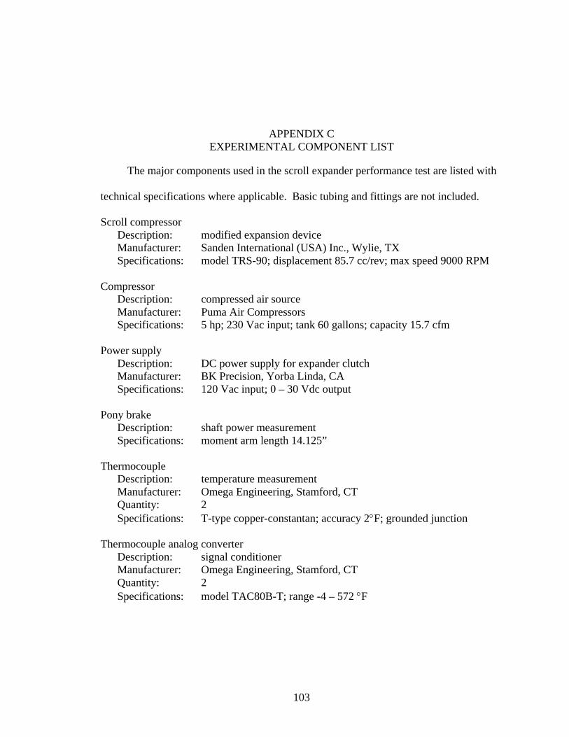
103

APPENDIX C EXPERIMENTAL COMPONENT LIST

The major components used in the scroll expander performance test are listed with

technical specifications where applicable. Basic tubing and fittings are not included.

Scroll compressor Description: modified expansion device Manufacturer: Sanden International (USA) Inc., Wylie, TX Specifications: model TRS-90; displacement 85.7 cc/rev; max speed 9000 RPM

Compressor

Description: compressed air source Manufacturer: Puma Air Compressors Specifications: 5 hp; 230 Vac input; tank 60 gallons; capacity 15.7 cfm

Power supply

Description: DC power supply for expander clutch Manufacturer: BK Precision, Yorba Linda, CA Specifications: 120 Vac input; 0 – 30 Vdc output

Pony brake

Description: shaft power measurement Specifications: moment arm length 14.125”

Thermocouple Description: temperature measurement

Manufacturer: Omega Engineering, Stamford, CT Quantity: 2 Specifications: T-type copper-constantan; accuracy 2°F; grounded junction Thermocouple analog converter

Description: signal conditioner Manufacturer: Omega Engineering, Stamford, CT Quantity: 2 Specifications: model TAC80B-T; range -4 – 572 °F

104

Multimeter Description: meter used to read thermocouple voltage Manufacturer: Fluke Corporation, Everett, WA Quantity: 2 Specifications: 0.01 mV resolution Pressure gauge

Description: pressure measurement Manufacturer: Campbell Hausfeld, Harrison, OH

Quantity: 2 Specifications: model IFA112; range 0 – 160 psig; resolution 1 psig Scale

Description: moment arm force measurement Manufacturer: Pelouze, Bridgeview, IL

Specifications: capacity 5lb; resolution 0.5 ounce; calibrated w/ standard masses Tachometer

Description: shaft rotational speed measurement

105

LIST OF REFERENCES

Barron, R. F., 1985, Cryogenic Systems, Oxford University Press, New York.

Casper, M. S., 1978, Hydrogen Production by Electrolysis, Thermal Decomposition and Unusual Techniques, Noyer Data Corporation, Park Ridge, NJ

Chevron U.S.A. Inc., 1998, “Diesel Fuel Refining and Chemistry,” San Ramon, CA. http://www.chevron.com/prodserv/fuels/bulletin/diesel/L2_4_6_rf.htm, last accessed: 11/2004.

Clean Energy Research Center, 2003, “Journey to Sustainable Energy: The H2 Solution,” University of South Florida, Tampa, FL. http://www.cerc.eng.usf.edu, last accessed: 11/2004.

Copeland Corp., 2001, “Scroll Compressor Technology and Air Conditioning, Heat Pump, and Refrigeration Applications,” Vi Ibero-American Congress of Air Conditioning and Refrigeration, Available at http://www.copeland-corp.com/americas/news/news004.htm/scroll-english.pdf

Drnevich, R., 2003, “Hydrogen Delivery: Liquefaction and Compression,” Hydrogen Delivery Workshop Proceedings, U.S. Department of Energy – Energy Efficiency and Renewable Energy, Washington, DC.

Energy Information Administration, 2003, “Annual Energy Review 2003,” DOE/EIA – 0384(2003), Washington, DC. http://www.eia.doe.gov/emeu/aer/contents.html, last accessed: 11/2004.

Energy Information Administration, 2004, “International Energy Outlook 2004,” Washington, DC. Available at http://www.eia.doe.gov/oiaf/ieo/world.html, last accessed: 11/2004.

Flynn, T. M., 1997, Cryogenic Engineering, Marcel Dekker, New York.

Fuel Cell Store, 2003, “Hydrogen Storage,” Boulder, CO. http://www.fuelcellstore.com/information/hydrogen_storage.html, last accessed: 11/2004.

Gater, R., 2001, Engineering Thermodynamics: Advanced Topics, Course notes, University of Florida, Gainesville, FL.

106

Goswami, D. Y., 1995, “Solar Thermal Power: Status of Technologies and Opportunities for Research,” Heat and Mass Transfer 95, Proceedings of the 2nd ASME-ISHMT Heat and Mass Transfer Conference, Tata-McGraw Hill Publishers, New Delhi, India, pp. 57 – 60.

Gravesen, J., Henriksen, C., 2001, “The Geometry of the Scroll Compressor,” SIAM Review, Vol. 43, No. 1, pp. 113-126.

Gross, R., Otto, W., Patzelt, A., Wanner, M., 1994, “Liquid Hydrogen for Europe – the Linde Plant at Ingolstadt,” Reports on Science and Technology, Linde, Vol. 54, pp. 37 – 43.

Hands, B. A., ed., 1986, Cryogenic Engineering, Academic Press, London.

Hans-Joachim, H., Radermacher, R., 2003, CO2 Compressor-Expander Analysis: Final Report, Air-Conditioning and Refrigeration Technology Institute, Arlington, VA, ARTI-21CR/611-10060-01.

Hasan, A. A., Goswami, D. Y., 2003, “ Exergy Analysis of a Combined Power and Refrigeration Thermodynamic Cycle Driven by a Solar Heat Source,” ASME Journal of Solar Energy Engineering, Vol. 125, No. 1, pp. 55 – 60.

Holman, J. P., Experimental Methods for Engineers, McGraw-Hill, New York.

McMurry, J., Fay, R., 1998, Chemistry, Prentice Hall Inc., Upper Saddle River, NJ.

Mirabal, S. T., 2003, “An Economic Analysis of Hydrogen Production Technologies Using Renewable Energy Resources,” Master’s thesis, University of Florida

National Hydrogen Association, 2004, “Hydrogen FAQs,” Washington, DC. http://www.hydrogenus.com/h2-FAQ.asp, last accessed: 11/2004.

National Institute of Standards and Technology, 2003, Program: Thermophysical Properties of Fluid Systems, http://webbook.nist.gov/chemistry/fluid/, last accessed: 11/2004.

Ramsay, W. C., 2003, Public-Private Dialogue, International Partnership for a Hydrogen Economy, International Energy Agency, Paris.

Schein, C., Radermacher, R., 2001, “Scroll Compressor Simulation Model,” ASME Journal of Engineering for Gas Turbines and Power, Vol. 123, pp. 217 – 225.

Stuart Energy Systems, 2004, “Stuart Energy Station Product Brochure,” Ontario, Canada. http://www.stuartenergy.com/main_our_products.html, last accessed: 11/2004.

107

Sunatech Inc., 2001, IEA Agreement on the Production and Utilization of Hydrogen, Task 12: Metal Hydrides and Carbon for Hydrogen Storage, Executive Summary, edited by Sandrock, U.S. Department of Energy, Washington, DC.

Tamm, G. O., 2003, “Experimental Investigation of an Ammonia-Based Combined Power and Cooling Cycle,” Ph.D. dissertation, University of Florida

Tamm, G., Goswami, D. Y., Lu, S., Hasan, A., “A Novel Combined Power and Cooling Thermodynamic Cycle for Low Temperature Heat Sources – Part I: Theoretical Investigation,” ASME Journal of Solar Energy Engineering, Vol. 125, No. 2, np.

Turns, S. R., 2000, An Introduction to Combustion: Concepts and Applications, McGraw-Hill, New York.

Wells, D. N., 2000, “Scroll Expansion Machines for Solar Power and Cooling Systems,” Proceedings of Solar 2000, American Society of Mechanical Engineers, Madison, WI, np.

Wendt, H., 1990, Electrochemical Hydrogen Technologies: Electrochemical Production and Combustion of Hydrogen, Elsevier Science Publishing, New York.

U.S. Department of Energy – Energy Efficiency and Renewable Energy, 2003, “Hydrogen Production,” Washington, DC. http://www.eere.energy.gov/RE/hydrogen_production.html, last accessed: 11/2004.

108

BIOGRAPHICAL SKETCH

Robert Joseph Reed was born in Baltimore, Maryland, in 1980. He graduated

summa cum laude from the University of Florida in 2003 with a B.S. degree in

mechanical engineering. He will graduate from the University of Florida in May 2005

with an M.S. degree. Robert is currently involved in the design and construction of a 5-

kW ammonia-based combined power and cooling cycle at the University of Florida

Energy Research Park.