Study on Preconditioned Conjugate Gradient Methodsfor Solving Large Sparse Matrix in CSR Format

(Course Project of ECE697NA)

Lin Du, Shujian Liu

April 30, 2015

Contents

1 Introdution 11.1 Methods for Solving System of Linear Equations . . . . . . . . . . . . . . . . 11.2 Background of Preconditioned Conjugate Gradient Methods . . . . . . . . . 21.3 Purpose of This Study . . . . . . . . . . . . . . . . . . . . . . . . . . . . . . 3

2 Conjugate Gradient Methods 42.1 Derivation of the Conjugate Gradient Methods . . . . . . . . . . . . . . . . . 42.2 Derivation of the Algorithm . . . . . . . . . . . . . . . . . . . . . . . . . . . 5

3 Preconditioned Conjugate Gradient Methods 63.1 Diagonal Matrix as the Preconditioner . . . . . . . . . . . . . . . . . . . . . 63.2 Split Preconditioner using Incomplete Cholesky Factorization . . . . . . . . . 6

4 Numerical Experiments 84.1 Matrices in Compress Row Storage Format . . . . . . . . . . . . . . . . . . . 84.2 Illustration of the Algorithms . . . . . . . . . . . . . . . . . . . . . . . . . . 84.3 Comparison of Two Incomplete Cholesky Factorization Subroutines . . . . . 104.4 Results and Discussion . . . . . . . . . . . . . . . . . . . . . . . . . . . . . . 11

5 Summary and Conclusions 16

Acknowledgements 17

References 18

Appendix A: Code 19

1 Introdution

1.1 Methods for Solving System of Linear Equations

A vast majority of problems in computational science and engineering are reduced to solvinga system of linear algebraic equations [1], which can be written in a matrix form, Ax = b.There are basically two classes of methods for solving the linear system. The first class isknown as direct methods, which theoretically give the exact solution in a finite number ofsteps. These methods have standard algorithms, are easy to incorporate in large softwares,and very efficient for solving small linear equation systems. For large systems, however, thisis not always true due to the inevitable round-off errors. Round-off errors made in one stepcan be brought into the next step, and continue to propogate to the end of the computing.If the system is very large, the accumulated round-off error may be so significant that thesolution is totally wrong. The direct solvers can not solve those nearly singular matrices.Even for those medium sized matrice, given the complexity of O(N3), the direct methodsmay be very time demanding, making them not the optimal option.

Though many modifications can be applied to the direct methods, to improve the prob-lems and enhance efficience, it is always a good idea to consider another class of methods,known as iterative methods, especially for a large sparse matrix which contains many zeros.The multiplicate with those zeros can be bypassed in the iterative methods. Since duringthe iteration, the sturcture of the matrix does not change, iterative methods require lessmemory than direct methods which need extra memory for fill-in’s. Last but not the least,the algorithms of iterative methods involve many matrix-vector multiplications, which ismake it very easy to be parallelized.

There are two major classes of iterative methods: (1) statinary iterative methods or fix-point iterations, and (2) projection methods. The stationary methods are named so becausethe solution to the linear equation system is expressed as finding a stationary point for theiteration x(k+1) = F (x(k)). The way to establish a convergence is to design a contraction, aproper mapping satisfying ‖F (x) − F (y)‖ < α(x − y), and α < 1. The convergence rate isdetermined by α. For a linear system Ax = b, it is easy to construct a iteration by split thecoefficient matrix A = M−N , substituting which into the linear system gives the importantResidual Form, x(k+1) = x(k) +M−1r(k). The choices of the matrix M correspond to a familyof standard iterative methods.

• Richardson (M = αI)

• Jacobi (M = D, D is the diagonal matrix formed by the diagonal elements of A.)

• Gauss-Seidel (M = (D + L), or the lower triangular of matrix A)

• Successive Over-Relaxation (M = (ω−1D + L), and ω > 1)a variant of the Gauss-Seidel method resulting in faster convergence. Values of ω < 1are often used to help establish convergence of a diverging iterative process or speedup the convergence of an overshooting process.

• Symmetric Successive Over-Relaxation (M = ω2−ω

(ω−1D + L)D−1(ω−1D + U))The symmetry of M permits the application of SSOR as a preconditioner for other

1

iterative schemes for symmetric matrices. This is the major motivation of the SSOR,since the convergence rate is usually slower than that of SOR.

The stationary iteration methods feature that the iterations are the same for each step,which makes the algorithms very simple. However, for real problems, the convergence of thisclassical iteration methods is usually very slow.

Another class of iterative methods are known as projection methods, the idea of whichis to extract an approximate solution from a subspace. The requirement of this method isthat the approximate solution x extracted from the subspace K should make the residualr = b − Ax orthogonal to the subspace L. If K = span(V ) and L = span(W ), whereV = [v1, v2, · · · , vm] and W = [w1, w2, · · · , wm], the expression of the approximate solutionis x = x0 + V (W TAV )−1W T r0. The simplest subspace is of course a straight line. Forsimplicity, we choose the V and W to be single vectors v and w, and successively approximatethe solution by the iteration x(k+1) = x(k) +αv, where α = wT r(k)

wTAv. Different choices of w and

v correspond to different methods:

• steepest descent method (v = r, and w = r)

• minimal residual method (v = r, and w = Ar)

• conjugate gradient method (v ∈ K, and w ∈ K)

• GMRES (v ∈ K, and w ∈ AK)

where the K = span[v,Av,A2v, · · · , Am−1v] is the Krylov subspace, because of which , thelast two methods are also known as Krylov subspace methods. Generally, the projectionmethods have better convergence properties compared with the classical stationary iterationmethods. In the rest of this report, we will focus on the study of conjugate gradient methodand the preconditioned conjugate gradient methods.

1.2 Background of Preconditioned Conjugate Gradient Methods

Conjugate gradient method was developed by Magnus R. Hestenes and Eduard Stiefel in1952 [2], under their effort for finding a machine method that satisfies properties of (1) beingsimple, (2) requiring a minimum of storage space, (3) converging rapidly preferably to aexact solution if no rounding-off errors occur, (4) being stable and able to self-correct byrepetition of the same routine, (5) using as many original data as possible in each step.They found that the CG method and the Gauss elimination method both satisfied the abovecriteria, and CG is superior to the elimination method as a machine method, for the reasonsthat

1. CG gives the exact solution in at most n steps if no rounding-off error occurs.

2. CG method is simple to code and less memory demanding

3. The matrix dose not change during the process, enabling the maximum usage of theoriginal data, and the preservation of the structure of the sparse coefficient matrices.

2

4. approximate solution given at each step is closer to the exact solution than the one atpreceding step

5. at each step one can start anew conveniently.

They also found interestingly that the CG and Gauss elimination are two special casesof a even broader method, conjugate direction method, which we will demonstrate in nextchapter.

CG method and its variants came into wide use only in the mid-1970, when vectorcomputers and massive computer memories were manufactured, which made it possible touse the CG methods to solve the problems including not only the linear equation systemsbut also nonlinear systems of equations and optimization problems. Since then, the CGalgorithm became an important basic tool for solving a wide variety problems [3].

1.3 Purpose of This Study

The purpose of this study is to demonstrate the derivation of the conjugate gradient method,the preconditioned CG, and the algorithms, to carry out numerical experiments by applyingthe CG and PCG to three linear systems with large sparse coefficient matrices, to discuss theefficiency of the CG and PCG by comparing the experiment results. Also discussed is theCompress Row Storage of large sparse matrices and its incomplete Cholesky factorization.As this is the course project of ECE697NA, we consider it a good opportunity to reviewall the methods, direct or iterative, we have learned in this class. Thus we summarized themajor methods for solving linear system of equations at the beginning of the report, in theintroduction section.

The structure of this report is following: Chapter 1 is the brief introduction of themajor numerical methods and the background of the CG and PCG methods; Chapter 2presents the derivation of the CG methods and the algorithms; Chapter 3 discusses the twopreconditioners for the CG methods; Chapter 4 is the experiments of solving large sparselinear system with the algorithms developed in sections 2 and 3; Chapter 5 is the summaryand conclusions.

We (Lin Du and Shujian Liu) cooperated closely on this project and had many discussionstogether or online, solved the difficulties together. It is hard to distinguish our efforts, totell who did what. We contributed equally to this project.

3

2 Conjugate Gradient Methods

2.1 Derivation of the Conjugate Gradient Methods

From the name of CG method we know there must be two key concepts involved in themethod: conjugate and gradient. Given a symmetric matrix A, two vectors d1 and d2 aresaid to be A-orthogonal or conjugate with respect to A, if dT1Ad2 = 0. A finite set of vectors{di} is a conjugate set if dTi Adj = 0 for all i 6= j. It is also easy to prove that if A is symetricpositive definit (spd), the conjugate set of vectors {di} are linearly independent [4]. Wewould see later on that the set of search directions in CG methods are a set of conjugatevectors with respect to the coefficent matrix A. Before introducing the concept of gradient,we need to introduce a functional

F =1

2xTAx+ bTx. (1)

We observe that the original equation

Ax+ b = 0 (2)

is equivalent to finding a point x that can minimize the functional of Eq. (1). The residualof the original equation is the gradient of the functional. This is where the concept gradientcomes into the picture.

Suppose the exact solution of Eq. (2) is x∗, and since {di} form a complete basis for thespace of Rn, we can express x∗ as

x∗ = α0d0 + α1d1 + · · ·+ αn−1dn−1, (3)

where αi are real numbers. Substituting Eq. (3) into Eq. (2) gives,

A(α0d0 + α1d1 + · · ·+ αn−1dn−1) + b = 0,

which multiplied with di gives

dTi A(α0d0 + α1d1 + · · ·+ αn−1dn−1) + dTi b = 0.

Due to the properties of conjugate vectors, we have

αi = − dTi b

dTi Adi, (4)

and

x∗ = −n−1∑i=0

dTi b

dTi Adidi. (5)

From computing αi one can see why we need conjugate set of vectors to form a basis, notmerely orthogonal ones. Upto this step, we should be very happy to see that if we can find{di}, then we can find the exact solution conviniently. The question now is how to constructthe mutually conjugate vectors.

4

We can start with a set of n linearly independent vectors u0, u1, · · · , un−1 and construct{di} by a successive A-orthogonalization process [2]. We use the formulas

d0 = u0,

d1 = u1 − α10u0,

d2 = u2 − α20u0 − α21u1,

...

di = ui − αi0u0 − αi1u1 − · · · − αi,i−1ui−1

...

The coefficient αij, (i > j) is to be chosen so that di is conjugate to dj. The formula for αij

is evidently

αij =(ui, Adj)

(dj, Adj)(j < i). (6)

If we select successively u0 = r0, u1 = r1, · · · , un−1 = rn−1, using the equations above wecan obtain a sequence of di, and xi. This procedure describes the conjugate gradient method.Interestingly, if one selects u0 = (1, 0, · · · , 0), u1 = (0, 1, · · · , 0), · · · , un−1 = (0, 0, · · · , 1),the procedure describes the Gauss elimination method. In next section, we will see how theabove analysis can lead to the CG algorithm.

2.2 Derivation of the Algorithm

From the previous section we can see the idea behind the CG algorithm. The algorithmwritten in pseudocode is given below [5].

1. x0 = 0, r0 = b− Ax0, d0 = r0.

2. For j = 0, 1, · · · , until convergence Do:

3. αj = (rj, rj)/(Adj, dj)

4. xj+1 = xj + αjdj

5. rj+1 = rj − αjAdj

6. βj+1 = (rj+1, rj+1)/(rj, rj)

7. dj+1 = rj+1 + βj+1dj

8. EndDo

5

3 Preconditioned Conjugate Gradient Methods

3.1 Diagonal Matrix as the Preconditioner

If the coefficient matrix A is ill-conditioned, the CG algorithm will still converge very slow.A work-around is to precondition the matrix A, with the purpose to reduce its conditionnumber. Below we give the preconditioned conjugate gradient method with the diagonalmatrix D being the preconditioner. D is formed by the diagonal elements of matrix A. Thealgorithm written in pseudocode is given below [5].

1. x0 = 0, r0 = b− Ax0, z0 = D−1r0, and d0 = z0.

2. For j = 0, 1, · · · , until convergence Do:

3. αj = (rj, zj)/(Adj, dj)

4. xj+1 = xj + αjdj

5. rj+1 = rj − αjAdj

6. zj+1 = D−1rj+1

7. βj+1 = (rj+1, zj+1)/(rj, zj)

8. dj+1 = zj+1 + βj+1dj

9. EndDo

3.2 Split Preconditioner using Incomplete Cholesky Factorization

We can also use split preconditioning technique to modify the matrix A. Assuming M isfactorized as: M = MLMR, the split preconditioning is

M−1L AM−1

R u = M−1L b, with x = M−1

R u.

Since the CG method required the coefficient matrix to be spd, a practical factorization isCholesky factorization, which is

M = LLT ,

where L is a lower triangular matrix. In this project, we will use the CG method to solvea large sparse linear system, meaning the matrix A will contain a large number of zeros.However, the result of Cholesky factorization L is not necessarily to be sparse. This mayrequire extra memories to store the fill-ins generated in the process of factorization. Anotherdown side is the factorization will take much time, slowing the algorithm. An alternativeapproach is to use incomplete Cholesky factorization method. This method and the algorithmwill be illustrated in next section. Here we assume that the matrix A has been factorized, andthe lower triangular matrix L has been obtained. The corresponding split precondtioningconjugate gradient algorithm written in pseudocode is given below [5].

1. x0 = 0, r0 = b− Ax0, r0 = L1r0, and d0 = L−T r0.

6

2. For j = 0, 1, · · · , until convergence Do:

3. αj = (rj, rj)/(Adj, dj)

4. xj+1 = xj + αjdj

5. rj+1 = rj − αjL−1Adj

6. βj = (rj+1, rj+1)/(rj, rj)

7. dj+1 = L−T rj+1 + βj+1dj

8. EndDo

7

4 Numerical Experiments

4.1 Matrices in Compress Row Storage Format

Many scientific or engineering problems, like boundary element method, will result in asystem of linear equation with a large sparse coefficient matrix, which contains a lot of zeros.Storing these zeros need a large amount of memories. However, these zeros literaly give noinformation. An efficient way to store the matrix is to keep only the non-zero elements in avector a, and record their coordinates in another two vectors ja and ia. Basically, there arethree ways of compress storage:

• COO ja stores the column numbers, ia stores the row numbers.

• CSR Compressed Sparse Row, ia stores only the beginning number of the first elementof each row.

• CSC Compressed Sparse Column, ja stores only the beginning number of the firstelement of each column.

Within above three approaches, the CSR is most efficient, and most popular. Thus, thethree matrices we will be used for numerical experiment are stored in this way. Though theCSR format can save a great amount of memories, the price is that more calculations will beinvolved, and the data locality is not as good as the traditional storage. One evidence is thatwe can not obtain the coordinate of element a(k) directly, or locate the a(k) for the elementof (i, j) directly. Mapping between k and (i, j) is needed. In next section, we shall write asubroutine to do this mapping, which will be used in the incomplete Cholesky factorizationalgorithm.

4.2 Illustration of the Algorithms

Up to now, we derived the algorithm of CG and PCG, which can be converted into Fortrancode easily. However, we haven’t obtained the algorithm of the incomplete Cholesky factor-ization applied on sparse matrix in CSR format. Incomplete Cholesky factorization is quitea standard one, and below is the algorithm written in Matlab code [6]:

function a = i c h o l ( a )n = s ize ( a , 1 ) ;

for k=1:na (k , k ) = sqrt ( a (k , k ) ) ;for i =(k+1):n

i f ( a ( i , k ) !=0)a ( i , k ) = a ( i , k )/ a (k , k ) ;

e nd i fendforfor j=(k+1):n

for i=j : ni f ( a ( i , j ) !=0)

a ( i , j ) = a ( i , j )−a ( i , k )∗ a ( j , k ) ;e nd i f

8

endforendfor

endfor

for i =1:nfor j=i +1:n

a ( i , j ) = 0 ;endfor

endforendfunct ion

However, this code is for the matrix of dense storage. To convert it to a version suitablefor the CSR matrix, we need to consider two things: (1) how to map a(k) with a(i, j), and(2) how to take advantage of the symmetry properties of the matrix A. For the question (1),we write a small subroutine iefinder(i,j,ie,ia,ja), which will give the correspondingelement number ie in the vector a, when the original coordinate (i, j) is given. The Fortrancode is:

subroutine i e f i n d e r ( i , j , i e , ia , j a )! Purpose : f i nd the va lue o f i e f o r sa ( i e )=a( i , j )

implicit noneInteger : : i , j , k , i e , i a (∗ ) , j a (∗ )

i e=0do k = ia ( i ) , i a ( i +1)−1

i f ( j a ( k ) . eq . j ) theni e = kexit

endifenddo

returnend subroutine i e f i n d e r

Before answering question (2), we observe that vector ia gives the ie of the non-zeroelements on a specific row, and ja will give the column number of those elements. Sincethe matrix A is symmetric, we can obtain the row numbers for those non-zero elements ina specific column as well. This information implies that we do not need to loop over all therows or columns to update the elements in each outer loop, as in the MATLAB code does,which has a computational cost of O(N3). We can actually use only one full loop (from 1 toN) to fulfill the incomplete Cholesky factorization. The Fortran code is:

subroutine i c h o l ( s l , ja , ia ,N)! Purpose : incomple te f a c t o r i z a t i o n o f CRS sparse matrix . L i s s t o r ed in the! lower t r i a n g u l a r par t o f s l and LˆT i s s t o r ed in the upper! t r i a n g u l a r par t o f s l .!! Arguments : akk (∗) s t o r e s the number o f d iagona l element , d iag ( k ) the index o f! o f the d iagona l e lement a ( k , k ) .! ja , i a and N are the same with those used in the main program .

implicit noneInteger : : N, i , j , k , i e , i e e i , i e e j , i e1 , i e2 , j a (∗ ) , i a (∗ ) , d iag ( 1 :N)

9

Double precision : : s l (∗ ) , akk

i e=0i e 1=0i e 2=0akk=0.d0

! f i n d the d iag element index i edo k=1,N

ca l l i e f i n d e r (k , k , i e , ia , j a )diag (k)= i e

enddo

do k=1, Ns l ( d iag (k))= sq r t ( s l ( d iag (k ) ) )akk=1.d0/ s l ( d iag (k ) )do i e e i=diag (k)+1 , i a ( k+1)−1 ! from the non−zero column # to

i=ja ( i e e i ) ! l o c a t e the non−zero row #ca l l i e f i n d e r ( i , k , i e , ia , j a )s l ( i e )= s l ( i e )∗ akkdo i e e j=i e +1, diag ( i ) ! update the row e lements o f lower t r i a n g u l a r

j=ja ( i e e j )ca l l i e f i n d e r ( i , k , i e1 , ia , j a )ca l l i e f i n d e r ( j , k , i e2 , ia , j a )i f ( ( i e 1 . ne . 0) . and . ( i e 2 . ne . 0 ) ) then

s l ( i e e j )= s l ( i e e j )− s l ( i e 1 )∗ s l ( i e 2 )endif

enddoenddo

enddo

! f i l l t he upper t r i a n g u l a r o f the matrix

do i =1, Ndo i e 1=diag ( i )+1 , i a ( i +1)−1

j=ja ( i e 1 )ca l l i e f i n d e r ( j , i , i e2 , ia , j a )s l ( i e 1 )= s l ( i e 2 )

enddoenddo

returnend subroutine i c h o l

The inner loops over ieei and ieej take advantage of the symmetry property of the matrixA, thus they do not need to go from 1 to N . This Fortran90 code can factorize the matricesvery quickly.

4.3 Comparison of Two Incomplete Cholesky Factorization Sub-routines

A subroutine of ICholeski has been provided to perform the incomplete Cholesky factoriza-tion of the cofficient matrix A. It is interesting to compare the efficiency of the ICholeski

10

with our own subroutine, ichol. In the code, we add a case4 for this comparison purpose,and perform the decomposition by the two subroutines sequentially and record the time.The results are listed in the table below

Table 1: The comparison of the efficiency of subroutines

Matrices N nnz ICholeski (s) ichol (s)gsmat1 432000 7955116 0.3734 0.9004laplace3d 180000 1211400 4.69× 10−2 6.39× 10−2

c6h6-vh 48913 1447514 0.1100 0.3317

We see that the provided subroutine ICholeski requires less time for the decompositionof the matrices. However, the performance of our subroutine ichol is also acceptable. Weused only one loop from 1 to N , which makes it of complexity of O(N). We do not knowthe source code of the subroutine ICholeski. From its description, we can see that it dealswith only the lower triangular of the orignal sparse matrices. In our subroutine, we dealwith the whole original matrices. Probably, this difference contributes to the difference inthe computing time. Though ichol needs a little more time, it also has some merits: (1) itdose not need the pre-treatment of the matrix, extracting the lower triangular of A; (2) itis simple and dose not need extra libraries; (3) it dose not need the extra memory for theextracted lower triangular matrix, thus is more memory efficient; (4) it outputs a matrixwith the same structure with the original one, thus vectors isa, jsa can be used directly;(5) it stores both the L and LT in the output matrix, which is very convenient in the PCGalgorithm, where LT is also needed. Considering those merits, we will use our own subroutineichol for the decomposition tasks in the following numerical experiments.

4.4 Results and Discussion

To investigate the efficiency of the algorithms of CG, the left preconditioned CG and the plitpreconditioned CG, we carried out numerical experiments upon three different large sparsematrices stored in the CSR format, which are gsmat1, laplace3d and c6h6-vh. The efficiencyis characterized by the number of iterations required for the convergence and the time ittakes. Once the normalized residual ‖r‖2/‖b‖2 < 10−14, the convergence is considered to bereached.

Figure 1 shows the normalized residual as a function of the iteration numbers. The blackline with open square markers is the result of conjugate gradient method, denoted by CG,the blue line with open circle markers is the result of preconditioned CG with the diagonalmatrix being the preconditioner, denoted by CG-D, and the red line with open trianglemarkers is for the split precondtioned conjugate gradient with the incomplete Choleskyfactorization matrix L as the preconditioner, denoted by CG-S. We observed that the line ofCG-D is almost overlapped with that of CG, and they require the same number of iterationsto achieve the convergence, indicating that the preconditioning with the diagonal matrix hasno effect on the coefficient matrix A. However, the CG-S line has a more steep slop thanthat of the CG and CG-D, and it reached 10−14 using 19 iterations, less than half of theiteration numbers for CG and CG-D. This shows that the split preconditioning with thematrix L improved the coefficient matrix A greatly, making it better conditioned.

11

1e-16

1e-14

1e-12

1e-10

1e-08

1e-06

0.0001

0.01

1

0 10 20 30 40 50 60

Norm

ali

zed R

esi

dual

Iteration

CGCG_DCG_S

Figure 1: The relative residual as a function of iteration numbers for matrix gsmat1.

0

1

2

3

4

5

6

0 10 20 30 40 50 60

Tim

e

Iterations

CGCG_DCG_S

Figure 2: The computing time as a function of iteration numbers for matrix gsmat1.

12

1e-16

1e-14

1e-12

1e-10

1e-08

1e-06

0.0001

0.01

1

100

0 20 40 60 80 100 120 140 160 180

Norm

ali

zed

Resi

dual

Iteration

CGCG_DCG_S

Figure 3: The relative residual as a function of iteration numbers for matrix laplace3d.

The computation time for CG, CG-D and CG-S is plotted as a function of iteration inthe Fig. 2. We see that though the CG-S required more iteration numbers to converge, ittook the least time to reach the convergence. CG-D required the same number of iterationsbut took a little more time to converge. This is because the preconditioning brought morecalculations into the algorithm. Since the multiplication with diagonal matrix is quite simple,the extra time it takes is also just a bit. However, the CG-S, though needed only 19 iterationsto converge, took almost twice the time of CG. This because the CG-S algorithm involvesin many more complicated calculations, like computing αjL

−1Adj and L−T rj+1 which needto be done by solving a system of linear equation. The matrix L has more complicatedstructure than D, which has also contributed to the long computation time.

We then carried out the numerical experiment on the matrix laplace3d. The residual v.s.iteration number is plotted in Fig. 3. Similar with the Fig. 1, the CG and CG-D completelyoverlap with each other, and took nearly 180 iterations to converge. The CG-S took only60 iterations to converge, showing a faster convergence speed. Compare with the result inFig. 1, CG-S saved more iterations for the matrix laplace3d.

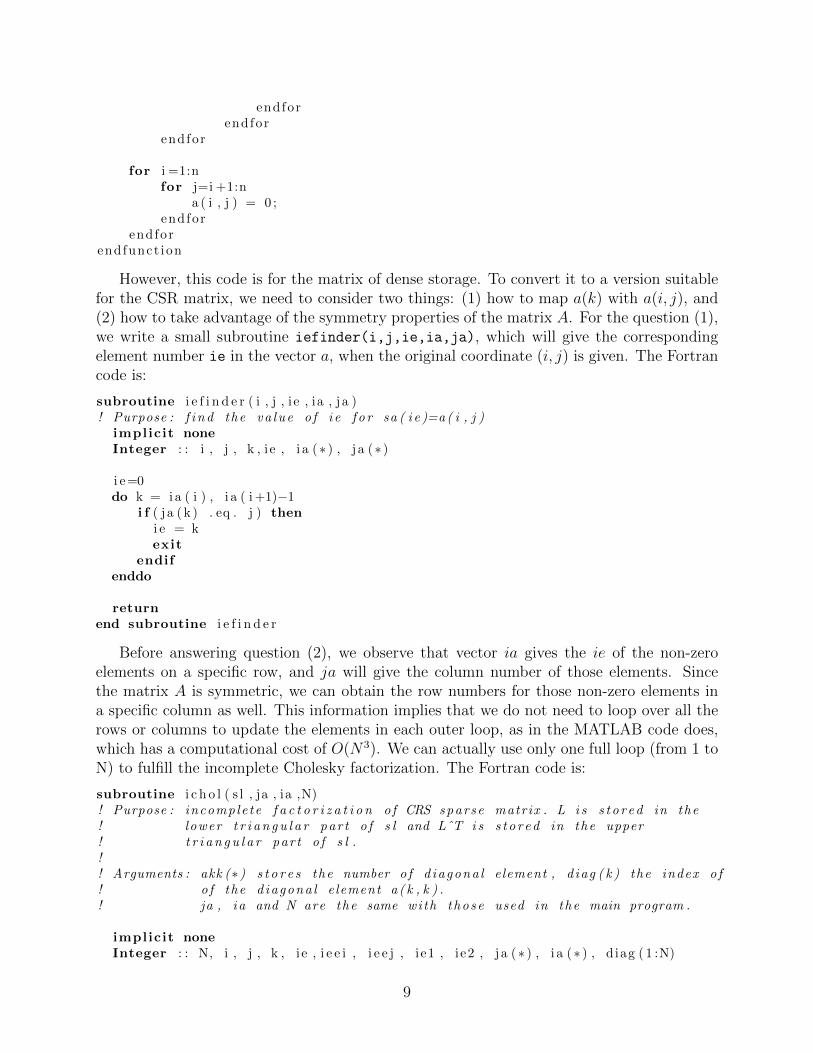
The computation time is plotted as a function of the iteration in Fig. 4. We can seethat though the CG has the least computation time, the CG-S took only a little more time.This implies that when the matrix A is more ill-preconditioned, the advantage that requiringfewer iterations to converge may make CG-S converge finally faster than CG.

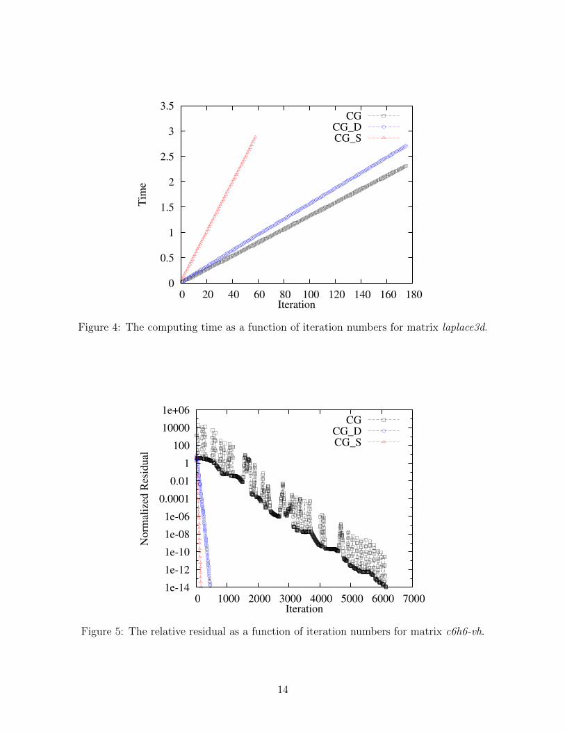
Finally we used our three algorithms to solve the third large sparse matrix c6h6-vh. Weplot the residual as a function of iteration in Fig. 5. This matrix is much larger and morecomplicated. The CG method took more than 6000 iterations to converge. The plot ofCG fluctuates greatly, which actually wastes a lot of iterations and computation time. Thepreconditioning with diagonal matrix has greatly improved the convergence. CG-D took 453iterations to converge. The CG-S took only 152 iterations to converge.

13

0

0.5

1

1.5

2

2.5

3

3.5

0 20 40 60 80 100 120 140 160 180

Tim

e

Iteration

CGCG_DCG_S

Figure 4: The computing time as a function of iteration numbers for matrix laplace3d.

1e-14

1e-12

1e-10

1e-08

1e-06

0.0001

0.01

1

100

10000

1e+06

0 1000 2000 3000 4000 5000 6000 7000

Norm

ali

zed R

esi

dual

Iteration

CGCG_DCG_S

Figure 5: The relative residual as a function of iteration numbers for matrix c6h6-vh.

14

0

10

20

30

40

50

60

70

80

0 1000 2000 3000 4000 5000 6000 7000

Tim

e

Iteration

CGCG_DCG_S

Figure 6: The computing time as a function of iteration numbers for matrix c6h6-vh.

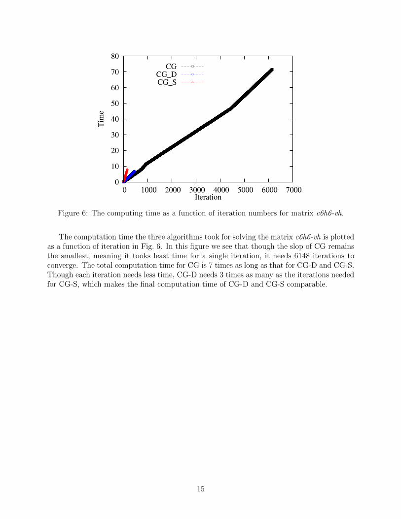
The computation time the three algorithms took for solving the matrix c6h6-vh is plottedas a function of iteration in Fig. 6. In this figure we see that though the slop of CG remainsthe smallest, meaning it tooks least time for a single iteration, it needs 6148 iterations toconverge. The total computation time for CG is 7 times as long as that for CG-D and CG-S.Though each iteration needs less time, CG-D needs 3 times as many as the iterations neededfor CG-S, which makes the final computation time of CG-D and CG-S comparable.

15

5 Summary and Conclusions

In this project, we reviewed the major methods for solving systems of linear equations(nonlinear equations can be reduced into linear equations as well). We focused our study onthe conjugate gradient (CG) method and different types of preconditioned conjugate gradient(PCG) methods. We derived mathematically the algorithm of the CG and PCG. We wroteFortran90 code to implement the algorithms. We derived two types of PCG algorithms: (1)CG-D, the PCG with preconditioner being the diagonal matrix D, and (2) CG-S, the PCGwith split preconditioners being the lower triangular matrix L (left preconditioner) and itstranspose LT (right preconditioner), where the L is obtained from the incomplete Choleskyfactorization of the coefficient matrix A.

We also discussed the three kinds of storage approaches for the large sparse matrix, andwrote a subroutine ichol in Fortran90 code for the incomplete Cholesky factorization formatrix in CSR format. We compare the efficiency of ichol with that of the provided subrou-tine ICholeski by comparing their computation time for decomposing three different largesparse matrices. The results show that ICholeski needs less time for the decomposition,and thus is more efficient. ichol is also very efficient. Considering other factors, we use ourown subroutine ichol to perform the factorization of the three matrices. Finally, we carriedout numerical experiments, using the three algorithms to solve three different large sparsematrices in CRS format, and compared the convergence speeds and the computation timeof the three algorithms.

Based on the analysis on the algorithm and the numerical experiment results, we drawthe major conclusions below:

1. Preconditioning usually can improve the convergence speed, making the algorithmconverge over fewer iterations.

2. Preconditioning makes the algorithm more complicated and require more calculationsfor a single iteration, thus increases the computation cost for one single iterations.

3. For well-conditioned matrix, both CG and PCG converge very quickly. CG is cheaperin overall computation cost than PCG. However, if the matrix is very ill-conditioned,PCG can converge much faster, and needs much less computation time than CG.

4. The split preconditioning with L and LT resulting from incomplete Cholesky factoriza-tion has better preconditioning effect than left preconditioning with diagonal matrixD.

16

Acknowledgements

We would like to express our deep appreciation to Professor Eric Polizzi, the instructor of thisvery interesting and extremely useful course ECE697NA, who has taught us many importantnumerical methods and inspired us to learn more, who spent much time on answering ourquestions and gave us many helpful suggestions on this project.

We also want to thank each other. We both work actively on this project, making thecooperation an enjoyable one.

17

References

[1] Constantine Pozrikidis. Numerical Computation in Science and Engineering. Oxford,2008.

[2] Magnus Hestenes and Eduard Stiefel. Methods of conjugate gradients for solving linearsystems. Journal of Research of the National Bureau of Standards, 49(6):409–436, 1952.

[3] Gene H. Golub and Dianne P. O’Leary. Some history of the conjugate gradient andlanczos algorithms:1948-1976*. Siam Reivew, 31(1):50–102, 1989.

[4] Yanbin Jia. Lecture note on conjugate gradient method, 2007.

[5] Yousef Saad. Iterative methods for sparse linear systems. Siam, 2003.

[6] Wikipedia. Incomplete cholesky factorization, 2015.

18

Appendix A: Code

program hw4

! ! ! ! ! ! ! v a r i a b l e d e c l a r a t i o nimplicit noneinteger : : i , j ,N, i t , itmax , k ,Nx ,Ny , e , nnz , n linteger : : i einteger : : t1 , t2 , timdouble precision : : hx , hy ,L , alpha , beta , pi , normr , normb , nres , errdouble precision , dimension ( : ) , allocatable : : sa , b , r ,dummy, x , s l , z , diag , l s ainteger , dimension ( : ) , allocatable : : i sa , j sa , l i s a , l j s acharacter ( len=100) : : name, a lgo! ! f o r banded s o l v e rdouble precision , dimension ( : , : ) , allocatable : : badouble precision : : nzero , norminteger : : kl , ku , i n f o! ! f o r pa rd i s ointeger ( 8 ) ,dimension (64) : : ptinteger , dimension (64) : : iparminteger : : mtypeinteger : : MAXFCT,MNUM,PHASE,MSGLVLinteger : : idumdouble precision , dimension ( : ) , allocatable : : usa , dinteger , dimension ( : ) , allocatable : : u isa , u j sa

! ! ! ! ! ! ! ! ! ! ! ! ! ! ! ! ! ! ! ! ! ! ! ! ! ! ! ! ! ! ! ! ! ! ! ! ! ! ! ! ! ! ! ! ! ! ! ! ! ! ! ! ! ! ! ! ! ! ! !! ! read command l i n e argument name=”1” ,”2” ,”3” ,”4” ,”5” , ”6” or ”7”

! ! ! ! ! ! ! ! ! ! ! ! ! ! ! ! ! ! ! ! ! ! ! ! ! ! ! ! ! ! ! ! ! ! ! ! ! ! ! ! ! ! ! ! ! ! ! ! ! ! ! ! ! ! ! ! ! ! ! !ca l l getarg (1 ,name)ca l l getarg (2 , a lgo )

! ! ! ! ! ! ! ! ! ! ! ! ! ! ! ! ! ! ! ! ! ! ! ! ! ! ! ! ! ! ! ! ! ! ! ! ! ! ! ! ! ! ! ! ! ! ! ! ! ! ! ! ! ! ! ! ! ! ! ! ! ! ! ! ! ! ! ! ! ! ! ! ! ! ! ! !! ! ! ! ! ! ! ! ! Read matr ix ”name” i s c s r format (3 ar ray s /3 f i l e s ) ! ! ! ! ! ! ! ! ! ! ! ! ! ! !! ! ! ! ! ! ! ! ! Create i sa , j sa , sa a r ray s ! ! ! ! ! ! ! ! ! ! ! ! ! ! ! ! ! ! ! ! ! ! ! ! ! ! ! ! ! ! ! ! ! ! ! ! ! ! ! !! ! ! ! ! ! ! ! ! ! ! ! ! ! ! ! ! ! ! ! ! ! ! ! ! ! ! ! ! ! ! ! ! ! ! ! ! ! ! ! ! ! ! ! ! ! ! ! ! ! ! ! ! ! ! ! ! ! ! ! ! ! ! ! ! ! ! ! ! ! ! ! ! ! ! ! !

open (10 , f i l e=trim (name)// ’ . i s a ’ , status=’ old ’ )read (10 ,∗ ) Nallocate ( i s a ( 1 :N+1))do i =1,N+1

read (10 ,∗ ) i s a ( i )end doclose (10)

open (10 , f i l e=trim (name)// ’ . j s a ’ , status=’ old ’ )read (10 ,∗ ) nnzallocate ( j s a ( 1 : nnz ) )do i =1,nnz

read (10 ,∗ ) j s a ( i )end doclose (10)

open (10 , f i l e=trim (name)// ’ . sa ’ , status=’ old ’ )read (10 ,∗ ) nnzallocate ( sa ( 1 : nnz ) )do i =1,nnz

read (10 ,∗ ) sa ( i )end doclose (10)

print ∗ , ’#’ , ’ Matrix : ’ , tr im (name)print ∗ , ’#’ , ’N=’ ,Nprint ∗ , ’#’ , ’ nnz=’ , nnzprint ∗ , ’ ’

! ! ! ! ! ! ! ! ! ! ! ! ! !

allocate (b ( 1 :N) ) ! ! R igh t hand−s i d eb=1.0d0

allocate ( x ( 1 :N) ) ! ! s o l u t i o nx=0.0d0 ! i n i t i a l s t a r t i n g v e c t o r

allocate ( r ( 1 :N) ) ! ! r e s i d u a l array

itmax=7000 ! i t e r a t i o n maximal a l l owederr=1d−14 ! convergence c r i t e r i a

allocate (dummy( 1 :N) ) ! ! dummy array i f a d d i t i o n a l s t o r a g e i s needed

select case ( a lgo )

case ( ”1” )! ! ! ! ! ! ! ! ! ! ! ! ! ! ! ! ! ! ! ! ! ! ! ! ! ! ! ! ! ! ! ! ! ! ! ! ! ! ! ! ! ! ! ! ! ! ! ! ! ! ! ! ! ! ! ! ! ! ! ! ! ! ! ! ! ! ! ! ! ! ! ! ! ! ! !

19

! ! ! ! ! ! ! ! Conjugate Gradient ! ! ! ! ! ! ! ! ! ! ! ! ! ! ! ! ! ! ! ! ! ! ! ! ! ! ! ! ! ! ! ! ! ! ! ! ! ! ! ! ! ! ! ! ! ! !! ! ! ! ! ! ! ! ! ! ! ! ! ! ! ! ! ! ! ! ! ! ! ! ! ! ! ! ! ! ! ! ! ! ! ! ! ! ! ! ! ! ! ! ! ! ! ! ! ! ! ! ! ! ! ! ! ! ! ! ! ! ! ! ! ! ! ! ! ! ! ! ! ! ! !

ca l l sys tem c lock ( t1 , tim )

! compute i n i t i a l r e s i d u a lr=bca l l dcsrmm( ’F ’ ,N,N,1 , −1.0d0 , sa , i sa , j sa , x , 1 . 0 d0 , r )nres=sum( abs ( r ) )/ sum( abs (b ) ) ! norm r e l a t i v e r e s i d u a l

! s ea rch d i r e c t i o n i n i t i a lallocate (d ( 1 :N) )d=r

i t=0do while ( ( nres>err ) . and . ( i t<itmax ) )

i t=i t+1 ! # o f i t e r a t i o n s

! A∗dca l l dcsrmm( ’F ’ ,N,N, 1 , 1 . 0 d0 , sa , i sa , j sa , d , 0 . 0 d0 ,dummy)

! a l pha=rˆ t . r /( dˆ t .A. d )alpha=sum( r ∗∗2)/sum(d∗dummy)

! x ( k)=x ( k−1)+a lpha ∗d ( k−1) ( new i t e r a t e )do i =1,N

x( i )=x( i )+alpha∗d( i )enddo

! b e t a =1/( r ˆ t . r )beta=1.d0/sum( r ∗∗2)

! new r e s i d u a l r=r−a lpha ∗A∗ddo i =1,N

r ( i )=r ( i )−alpha∗dummy( i )enddo

! norm r e l a t i v e r e s i d u a lnres=sum( abs ( r ) )/ sum( abs (b ) )

! b e t a v a l u e updatedbeta=beta∗sum( r ∗∗2)

! Update s earch d i r e c t i o n d=r+be t a ∗ddo i =1,N

d( i )=r ( i )+beta∗d( i )enddo

ca l l sys tem c lock ( t2 , tim ) ! f i n a l t ime

print ∗ , i t , nres , ( t2−t1 )∗1 .0 d0/timend do

case ( ”2” )! ! ! ! ! ! ! ! ! ! ! ! ! ! ! ! ! ! ! ! ! ! ! ! ! ! ! ! ! ! ! ! ! ! ! ! ! ! ! ! ! ! ! ! ! ! ! ! ! ! ! ! ! ! ! ! ! ! ! ! ! ! ! ! ! ! ! ! ! ! ! ! ! ! ! !! ! ! ! ! ! ! ! P r e cond i t i oned Conjugate Gradient ( Diagona l ) ! ! ! ! ! ! ! ! ! ! ! ! ! ! ! ! ! ! ! ! ! ! !! ! ! ! ! ! ! ! ! ! ! ! ! ! ! ! ! ! ! ! ! ! ! ! ! ! ! ! ! ! ! ! ! ! ! ! ! ! ! ! ! ! ! ! ! ! ! ! ! ! ! ! ! ! ! ! ! ! ! ! ! ! ! ! ! ! ! ! ! ! ! ! ! ! ! !

! ! ! ! e x t r a c t d i a g ona l matr ix ( s t o r e t h e i n v e r s e o f t h e d i a g ona l e l emen t s )allocate ( diag ( 1 :N) )do k=1,N

do i=i s a (k ) , i s a (k+1)−1i f ( j s a ( i ) == k) then

diag (k)=1.d0/ sa ( i )exit

elsediag (k)=0.d0

endifenddo

enddo

ca l l sys tem c lock ( t1 , tim )

! compute i n i t i a l r e s i d u a lr=bca l l dcsrmm( ’F ’ ,N,N,1 , −1.0d0 , sa , i sa , j sa , x , 1 . 0 d0 , r )nres=sum( abs ( r ) )/ sum( abs (b ) ) ! norm r e l a t i v e r e s i d u a l! compute z 0 s t o r e d in zallocate ( z ( 1 :N) )z=r∗diag

! s ea rch d i r e c t i o n i n i t i a lallocate (d ( 1 :N) )d=z

i t=0do while ( ( nres>err ) . and . ( i t<itmax ) )

i t=i t+1 ! # o f i t e r a t i o n s

! A∗d

20

ca l l dcsrmm( ’F ’ ,N,N, 1 , 1 . 0 d0 , sa , i sa , j sa , d , 0 . 0 d0 ,dummy)

! a l pha=rˆ t . z /( dˆ t .A. d )alpha=sum( r∗z )/sum(d∗dummy)

! x ( k)=x ( k−1)+a lpha ∗d ( k−1) ( new i t e r a t e )x=x+alpha∗d

! b e t a =1/( r ˆ t . z )beta=1.d0/sum( r∗z )

! new r e s i d u a l r=r−a lpha ∗A∗dr=r−alpha∗dummy

! new z z=Mˆ−1. rz=r∗diag

! norm r e l a t i v e r e s i d u a lnres=sum( abs ( r ) )/ sum( abs (b ) )

! b e t a v a l u e updatedbeta=beta∗sum( r∗z )

! Update s earch d i r e c t i o n d=z+be t a ∗dd=z+beta∗d

ca l l sys tem c lock ( t2 , tim ) ! f i n a l t ime

print ∗ , i t , nres , ( t2−t1 )∗1 .0 d0/timend do

case ( ”3” )! ! ! ! ! ! ! ! ! ! ! ! ! ! ! ! ! ! ! ! ! ! ! ! ! ! ! ! ! ! ! ! ! ! ! ! ! ! ! ! ! ! ! ! ! ! ! ! ! ! ! ! ! ! ! ! ! ! ! ! ! ! ! ! ! ! ! ! ! ! ! ! ! ! ! !! ! ! ! ! ! ! ! P r e cond i t i oned Conjugate Gradient ( s p l i t p r e c on d i t i o n e r ) ! ! ! ! ! ! ! ! ! ! !! ! ! ! ! ! ! ! ! ! ! ! ! ! ! ! ! ! ! ! ! ! ! ! ! ! ! ! ! ! ! ! ! ! ! ! ! ! ! ! ! ! ! ! ! ! ! ! ! ! ! ! ! ! ! ! ! ! ! ! ! ! ! ! ! ! ! ! ! ! ! ! ! ! ! !

! ! ! ! i n comp l e t e f a c t o r i z a t i o n o f A and s t o r e L in s lallocate ( s l ( 1 : nnz ) )s l=sa

ca l l i c h o l ( s l , j sa , i sa ,N)

ca l l sys tem c lock ( t1 , tim )

! compute i n i t i a l r e s i d u a lr=bca l l dcsrmm( ’F ’ ,N,N,1 , −1.0d0 , sa , i sa , j sa , x , 1 . 0 d0 , r )nres=sum( abs ( r ) )/ sum( abs (b ) ) ! norm r e l a t i v e r e s i d u a l

! compute r h a t=Lˆ−1 r ( r e s i d u a l i n i t i a l )ca l l dcsr sv ( ’L ’ ,N, 1 , s l , i sa , j sa , r )

! compute d 0 = Lˆ−T r h a t ( s ea rch d i r e c t i o n i n i t i a l )allocate (d ( 1 :N) )d=rca l l dcsr sv ( ’U ’ ,N, 1 , s l , i sa , j sa , d)

i t=0do while ( ( nres>err ) . and . ( i t<itmax ) )

i t=i t+1 ! # o f i t e r a t i o n s

! A∗dca l l dcsrmm( ’F ’ ,N,N, 1 , 1 . 0 d0 , sa , i sa , j sa , d , 0 . 0 d0 ,dummy)

! a l pha=rˆ t . r /( dˆ t .A. d )alpha=sum( r ∗∗2)/sum(d∗dummy)

! x ( k)=x ( k−1)+a lpha ∗d ( k−1) ( new i t e r a t e )do i =1,N

x( i )=x( i )+alpha∗d( i )enddo

! b e t a =1/( r ˆ t . r ) b e f o r e r b e in g o v e rw r i t t e n and f o r use l a t e r onbeta=1.d0/sum( r ∗∗2)

! compute dummy=Lˆ−1.A. dca l l dcsr sv ( ’L ’ ,N, 1 , s l , i sa , j sa ,dummy)

! new r e s i d u a l r=r−a lpha ∗A∗dr=r−alpha∗dummy

! compute t h e o r i g i n a l r e s i d u a l dummy=L . r h a tca l l dcsrmm( ’L ’ ,N,N, 1 , 1 . 0 d0 , s l , i sa , j sa , r , 0 . 0 d0 ,dummy)

! norm r e l a t i v e r e s i d u a lnres=sum( abs (dummy))/ sum( abs (b ) )

! b e t a v a l u e updatedbeta=beta∗sum( r ∗∗2)

! compute dummy=Lˆ−T. r

21

dummy=rca l l dcsr sv ( ’U ’ ,N, 1 , s l , i sa , j sa ,dummy)

! Update s earch d i r e c t i o n d=Lˆ−T. r+be t a ∗dd=dummy+beta∗d

ca l l sys tem c lock ( t2 , tim ) ! f i n a l t ime

print ∗ , i t , nres , ( t2−t1 )∗1 .0 d0/timend do

case ( ”4” )! ! ! ! ! ! ! ! ! ! ! ! ! ! ! ! ! ! ! ! ! ! ! ! ! ! ! ! ! ! ! ! ! ! ! ! ! ! ! ! ! ! ! ! ! ! ! ! ! ! ! ! ! ! ! ! ! ! ! ! ! ! ! ! ! ! ! ! ! ! ! ! ! ! ! !! ! ! ! Comparison o f t h e two Algo . o f i n comp l e t e Cho l e sky f a c t o r i z a t i o n ! ! ! ! ! ! !! ! ! ! ! ! ! ! ! ! ! ! ! ! ! ! ! ! ! ! ! ! ! ! ! ! ! ! ! ! ! ! ! ! ! ! ! ! ! ! ! ! ! ! ! ! ! ! ! ! ! ! ! ! ! ! ! ! ! ! ! ! ! ! ! ! ! ! ! ! ! ! ! ! ! !

! ! ! ! my own a l g o r i t hm as in s u b r ou t i n e i c h o l! ! ! ! i n comp l e t e f a c t o r i z a t i o n o f A and s t o r e bo th L and LˆT in s l

ca l l sys tem c lock ( t1 , tim )allocate ( s l ( 1 : nnz ) )s l=sa

ca l l i c h o l ( s l , j sa , i sa ,N)ca l l sys tem c lock ( t2 , tim )

print ∗ , ”Time used by i c h o l i s : ” , ( t2−t1 )∗1 .0 d0/timdeallocate ( s l )

! ! ! ! t h e a l g o r i t hm prov ided , ICho l e s k y . o! ! ! ! The lower t r i a n g u l a r o f A needs to be e x t r a c t e d to s t o r e in ano ther CSR! ! ! ! format l s a , l i s a , l j s a . This i s down by s u b r ou t i n e d c s r 2 c s r l ow , which i s! ! ! ! p r o v i d ed in t he l i b r a r y o f d z l s p r im . Then the s u b r ou t i n e ICho l e s k i w i l l! ! ! ! per form the decompos i t i on on l sa , and s t o r e t h e matr ix L in s l , which can! ! ! ! share t h e c oo r d i na t e v e c t r o s , l i s a and l j s a w i th l s a .

ca l l sys tem c lock ( t1 , tim )nl=(nnz+n)/2 ! number o f elem in l s aallocate ( l s a ( 1 : n l ) )allocate ( l i s a ( 1 :N+1))allocate ( l j s a ( 1 : n l ) )allocate ( s l ( 1 : n l ) )

! e x t r a c t t h e l ower t r i a n g u l a rca l l dc s r 2 c s r l ow (0 ,N, sa , i sa , j sa , l sa , l i s a , l j s a )

! d ecompos i t i onca l l ICho l e sk i (N, l sa , l i s a , l j s a , s l )

ca l l sys tem c lock ( t2 , tim ) ! f i n a l t ime

print ∗ , ”Time used by ICho l e sk i i s : ” , ( t2−t1 )∗1 .0 d0/tim

! ! ! ! ! ! ! ! ! ! ! ! ! ! ! ! ! ! ! ! ! ! ! ! ! ! ! ! ! ! ! ! ! ! ! ! ! ! ! ! ! ! ! ! ! ! ! ! ! ! ! ! ! ! ! ! ! ! ! !end select

print ∗ , ’ ’i f ( i t>=itmax ) then

print ∗ , ’#’ , ’∗∗Attent ion ∗∗ did not converge to ’ , err , ’ a f t e r ’ , itmax , ’ i t e r a t i o n s ’else

i f ( i t /=0) thenprint ∗ , ’#’ , ’ Success− converge below ’ , err , ’ in ’ , i t , ’ i t e r a t i o n s ’

elseprint ∗ , ’#’ , ’ D i rec t so lve r− r e s i d u a l ’ , nres

endifend i f

print ∗ , ’#’ , ’ Total time ’ , ( t2−t1 )∗1 .0 d0/tim

end program hw4

22