www.ijcrt.org © 2018 IJCRT | Volume 6, Issue 2 April 2018 | ISSN: 2320-2882

IJCRT1813014 International Journal of Creative Research Thoughts (IJCRT) www.ijcrt.org 1123

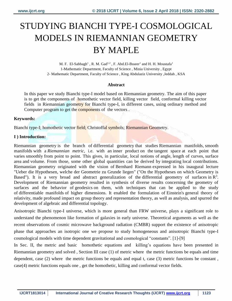
STUDYING BIANCHI TYPE-I COSMOLOGICAL

MODELS IN RIEMANNIAN GEOMETRY

BY MAPLE

M. F. El-Sabbagh1 , R. M. Gad1,2 , F. Abd.El-Bsseer1 and H. H. Moustafa1

1-Mathematic Department, Faculty of Science , Minia University , Egypt

2- Mathematic Department, Faculty of Science , King Abdulaziz University ,Jeddah , KSA

Abstract

In this paper we study Bianchi type-I model based on Riemannian geometry. The aim of this paper

is to get the components of homothetic vector field, killing vector field, conformal killing vector

fields in Riemannian geometry for Bianchi type-I, in different cases, using ordinary method and

Computer program to get the components of the vectors .

Keywords:

Bianchi type-I; homothetic vector field; Christoffal symbols; Riemannian Geometry.

I ) Introduction:

Riemannian geometry is the branch of differential geometry that studies Riemannian manifolds, smooth

manifolds with a Riemannian metric, i.e. with an inner product on the tangent space at each point that

varies smoothly from point to point. This gives, in particular, local notions of angle, length of curves, surface

area and volume. From those, some other global quantities can be derived by integrating local contributions.

Riemannian geometry originated with the vision of Bernhard Riemann expressed in his inaugural lecture

"Ueber die Hypothesen, welche der Geometrie zu Grunde liegen" ("On the Hypotheses on which Geometry is

Based"). It is a very broad and abstract generalization of the differential geometry of surfaces in R3.

Development of Riemannian geometry resulted in synthesis of diverse results concerning the geometry of

surfaces and the behavior of geodesics on them, with techniques that can be applied to the study

of differentiable manifolds of higher dimensions. It enabled the formulation of Einstein's general theory of

relativity, made profound impact on group theory and representation theory, as well as analysis, and spurred the

development of algebraic and differential topology.

Anisotropic Bianchi type-I universe, which is more general than FRW universe, plays a significant role to

understand the phenomenon like formation of galaxies in early universe. Theoretical arguments as well as the

recent observations of cosmic microwave background radiation (CMBR) support the existence of anisotropic

phase that approaches an isotropic one we propose to study homogeneous and anisotropic Bianchi type-I

cosmological models with time dependent gravitational and cosmological “constants”. [1]-[9]

In Sec. II, the metric and basic homothetic equations and killing’s equations have been presented in

Riemannian geometry and solved , Section III case (1) of metric where the metric functions be equals and time

dependent, case (2) where the metric functions be equals and equal t, case (3) metric functions be constant ,

case(4) metric functions equals one , get the homothetic, killing and conformal vector fields.

www.ijcrt.org © 2018 IJCRT | Volume 6, Issue 2 April 2018 | ISSN: 2320-2882

IJCRT1813014 International Journal of Creative Research Thoughts (IJCRT) www.ijcrt.org 1124

Problem statement and objectives:

Where studying some of the models of metric space times in the Riemannian geometry it is difficult to get

homothetic equations as well as to get solved. In this paper we calculate the equations in the ordinary method as

well as using a computer program and compare the results to be able to use computer programs in difficult

models.

Methods: In this paper we get homothetic equations by equation (II.3). We solve the partial differential

equations by separate variables and use Maple 17 program for getting the homothetic vector field.

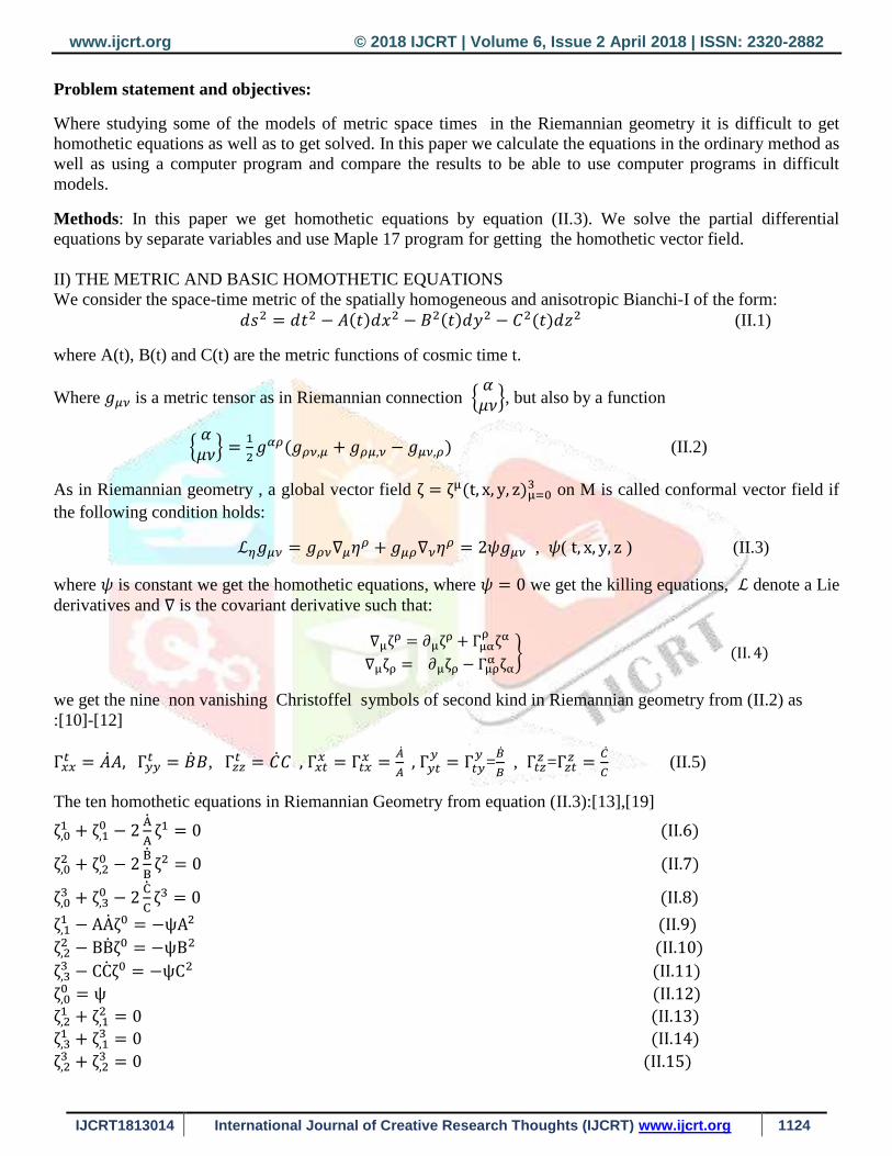
II) THE METRIC AND BASIC HOMOTHETIC EQUATIONS

We consider the space-time metric of the spatially homogeneous and anisotropic Bianchi-I of the form:

𝑑𝑠2 = 𝑑𝑡2 − 𝐴(𝑡)𝑑𝑥2 − 𝐵2(𝑡)𝑑𝑦2 − 𝐶2(𝑡)𝑑𝑧2 (II.1)

where A(t), B(t) and C(t) are the metric functions of cosmic time t.

Where 𝑔𝜇𝜈 is a metric tensor as in Riemannian connection {𝛼

𝜇𝜈}, but also by a function

{𝛼

𝜇𝜈} =1

2𝑔𝛼𝜌(𝑔𝜌𝜈,𝜇 + 𝑔𝜌𝜇,𝜈 − 𝑔𝜇𝜈,𝜌) (II.2)

As in Riemannian geometry , a global vector field ζ = ζμ(t, x, y, z)μ=03 on M is called conformal vector field if

the following condition holds:

ℒ𝜂𝑔𝜇𝜈 = 𝑔𝜌𝜈∇𝜇𝜂𝜌 + 𝑔𝜇𝜌∇𝜈𝜂𝜌 = 2𝜓𝑔𝜇𝜈 , 𝜓( t, x, y, z ) (II.3)

where 𝜓 is constant we get the homothetic equations, where 𝜓 = 0 we get the killing equations, ℒ denote a Lie

derivatives and ∇ is the covariant derivative such that:

∇μζρ = ∂μζρ + Γμα

ρζα

∇μζρ = ∂μζρ − Γμρα ζα

} (II. 4)

we get the nine non vanishing Christoffel symbols of second kind in Riemannian geometry from (II.2) as

:[10]-[12]

Γ𝑥𝑥𝑡 = ��𝐴, Γ𝑦𝑦

𝑡 = ��𝐵, Γ𝑧𝑧𝑡 = ��𝐶 , Γ𝑥𝑡

𝑥 = Γ𝑡𝑥𝑥 =

��

𝐴 , Γ𝑦𝑡

𝑦= Γ𝑡𝑦

𝑦=

��

𝐵 , Γ𝑡𝑧

𝑧 =Γ𝑧𝑡𝑧 =

��

𝐶 (II.5)

The ten homothetic equations in Riemannian Geometry from equation (II.3):[13],[19]

ζ,01 + ζ,1

0 − 2A

A

ζ1 = 0 (II.6)

ζ,02 + ζ,2

0 − 2B

B

ζ2 = 0 (II.7)

ζ,03 + ζ,3

0 − 2C

C

ζ3 = 0 (II.8)

ζ,11 − AAζ0 = −ψA2 (II.9)

ζ,22 − BBζ0 = −ψB2 (II.10)

ζ,33 − CCζ0 = −ψC2 (II.11)

ζ,00 = ψ (II.12)

ζ,21 + ζ,1

2 = 0 (II.13)

ζ,31 + ζ,1

3 = 0 (II.14)

ζ,23 + ζ,2

3 = 0 (II.15)

www.ijcrt.org © 2018 IJCRT | Volume 6, Issue 2 April 2018 | ISSN: 2320-2882

IJCRT1813014 International Journal of Creative Research Thoughts (IJCRT) www.ijcrt.org 1125

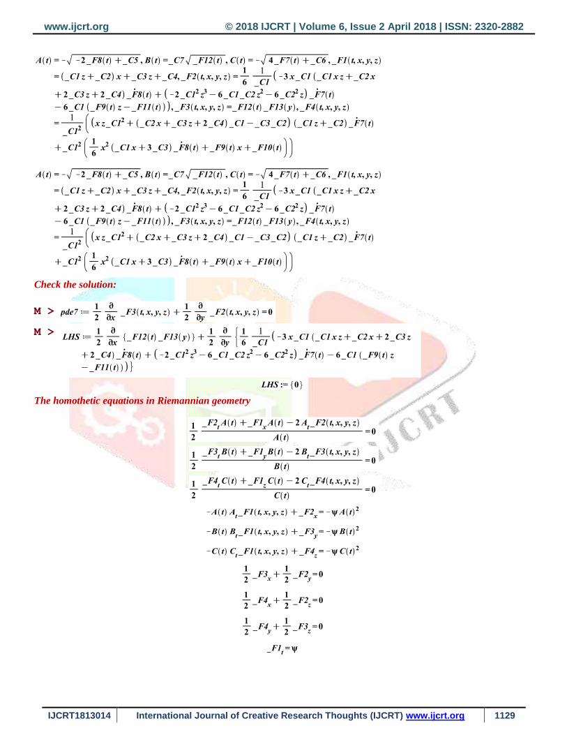
The solution of the homothetic equations see Appendix(1)is: [20]

A(t) = −√−f8(t)

2ψ, B(t) = √

−C1

2ψ, C(t) = √

−C2

2ψ, ζ1 = −f10,x

(t, x)y − f12,x(t, x)z

ζ2 = f8(t)z + c1y + f10(t, x),ζ3 = −f8(t)y + c2y + f12(t, x),ζ0 = ψt + f2(x, y, z) Where 𝑐𝑖 , i=1,2,…are the integration constants and 𝑓𝑖 , i=1,2,…the integration functions

The homothetic vector fields is:

ζ = [ψt + f2(x, y, z)] ∂t + [−f10,x(t, x)y − f12,x

(t, x)z] ∂x+[f8(t)z + c1y + f10(t, x)] ∂y + [−f8(t)y + c2y +

f12(t, x)] ∂z

The solution of the killings equations:

𝐴(𝑡) = √𝑐5 − 2𝑓8(𝑡), 𝐵(𝑡) = 𝑐7√𝑓12(𝑡) , 𝐶(𝑡) = −√𝑐6 + 4𝑓7(𝑡)

𝜁0 = (𝑐1𝑧 + 𝑐2)𝑥 + 𝑐3 + 𝑐4 , 𝜁2 = 𝑓12(𝑡)𝑓13(𝑦)

𝜁1 =1

6𝑐1[−3𝑥𝑐1𝑓8(𝑡)(𝑐1𝑥𝑧 + 𝑐2𝑥 + 2𝑐3𝑧 + 2𝑐4) − 2𝑧𝑓7(𝑡)(𝑐1

2𝑧2 + 3𝑐1𝑐2 + 3𝑐22) − 6𝑐1(𝑓9(𝑡)𝑧 − 𝑓11(𝑡))],

𝜁3 =1

𝑐12 [(𝑥𝑧𝑐1

2 + (𝑐2𝑥 + 𝑐3𝑧 + 2𝑐4)𝑐1 − 𝑐2𝑐3)(𝑐2 + 𝑐1𝑧) 𝑓7(𝑡) + 𝑐12 (

𝑥2

6(𝑐1𝑥 + 3𝑐3)𝑓8(𝑡) + 𝑓9(𝑡)𝑥 + 𝑓10(𝑡))]

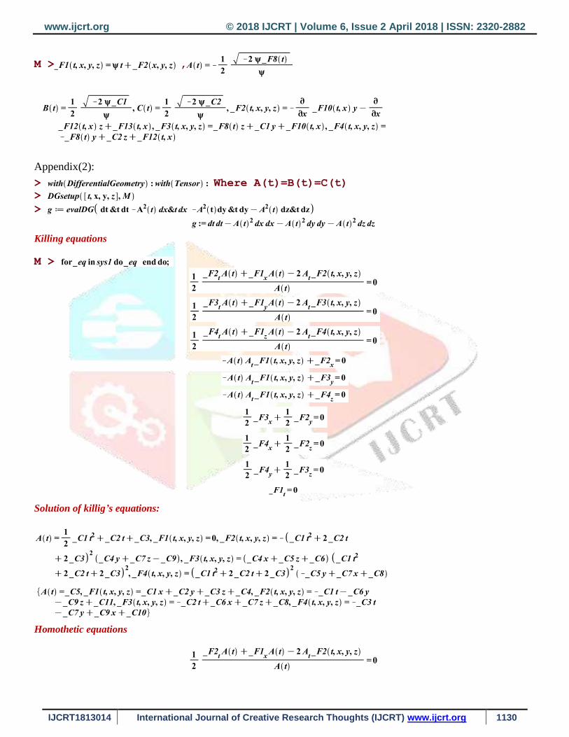
III) Case(1):

In the case where 𝐴(𝑡) = 𝐵(𝑡) = 𝐶(𝑡) the metric be as: 𝑑𝑠2 = 𝑑𝑡2 − 𝐴2(𝑡)(𝑑𝑥2 + 𝑑𝑦2 + 𝑑𝑧2)

The homothetic equations will has the solution Appendix( 2):

𝐴(𝑡) = 𝑐4 , 𝜁0 = 𝑐1𝑥 + 𝑐2𝑦 + 2𝜓𝑡 + 𝑐3, 𝜁1 = 𝑐5𝑦+𝑐6𝑧 − 𝑐1𝑡 − 2𝑐42𝜓𝑥 + 𝑐7

𝜁2 = 𝑐8𝑧 − 𝑐2𝑡 − 𝑐5𝑥 − 2𝑐42𝜓𝑦 + 𝑐9,𝜁3 = 𝑐10 − 𝑐8𝑦 − 𝑐2𝑡 − 2𝑐4

2𝜓𝑧 − 𝑐6𝑥

Homothetic vector fields is:

𝜁 = [𝑐1𝑥 + 𝑐2𝑦 + 2𝜓𝑡 + 𝑐3]𝜕𝑡 + [𝑐5𝑦+𝑐6𝑧 − 𝑐1𝑡 − 2𝑐42𝜓𝑥 + 𝑐7]𝜕𝑥+[𝑐8𝑧 − 𝑐2𝑡 − 𝑐5𝑥 − 2𝑐4

2𝜓𝑦 + 𝑐9]𝜕𝑦 + [𝑐10 −𝑐8𝑦 − 𝑐2𝑡 − 2𝑐4

2𝜓𝑧 − 𝑐6𝑥]𝜕𝑧

The killing’s equations has the solution:

A(t) =c1

2t2 + c2t + c3 , ζ0 = 0, ζ1 = (c9 − c4y−c7z)(c1t2 + 2c2t + 2c3)2

ζ2 = (c6 + c4x+c5z)(c1t2 + 2c2t + 2c3)2,ζ3 = (c8 − c5y+c7x)(c1t2 + 2c2t + 2c3)2

The killing vector field:

𝜁 = (𝑐1𝑡2 + 2𝑐2𝑡 + 2𝑐3)2{0𝜕𝑡 + (𝑐9 − 𝑐4𝑦−𝑐7𝑧)𝜕𝑥+(𝑐6 + 𝑐4𝑥+𝑐5𝑧)𝜕𝑦 + (c8 − c5y+c7x) ∂z}

Case(2): In the case where A(t) = B(t) = C(t)=t the metric be as: ds2 = dt2 − t2(dx2 + dy2 + dz2)

The solution of homothetic equations see appendix(3) be:

www.ijcrt.org © 2018 IJCRT | Volume 6, Issue 2 April 2018 | ISSN: 2320-2882

IJCRT1813014 International Journal of Creative Research Thoughts (IJCRT) www.ijcrt.org 1126

𝜁0 = 2𝜓𝑡, 𝜁1 = (𝑐1𝑦 + 𝑐2𝑧 + 𝑐3)𝑡2, 𝜁2 = (𝑐4𝑧 − 𝑐1𝑥 + 𝑐5)𝑡2, 𝜁3 = (𝑐6 − 𝑐2𝑥 − 𝑐4𝑦)𝑡2

Homothetic vector fields is:

ζ = 2ψt ∂t + [(c1y + c2z + c3)t2] ∂x+[(c4z − c1x + c5)t2] ∂y + [(c6 − c2x − c4y +)t2] ∂z

The solution of killing’s equations is:

ζ0 = 0, ζ1 = (c1y + c2z + c3)t2, ζ2 = (c4z − c1x + c5)t2, ζ3 = (c6 − c2x − c4y)t2

The killing vector field:

ζ = 0 ∂t + [(c1y + c2z + c3)t2] ∂x+[(c4z − c1x + c5)t2] ∂y + [(c6 − c2x − c4y +)t2] ∂z

The solution of conformal equations:

ψ(t, x, y, z) =1

4[ln(t2)c1 + 2ln(t)(c3z + c5x + c7y + c1 + c8) + c1(x2 + y2 + z2) + 2x(c4 + c5) + 2y(c6 + c7)

+ 2z(c2 + c3) +1

2(c8 + c)]

ζ0 = t [1

2ln(t2)c1 + ln(t)(c3z + c5x + c7y + c8) +

c1

2(x2 + y2 + z2) + c6y + c4x + c2z + c9]

ζ1 =t2

2[ln(t2)c5 + 2x(c1ln(t)+c3z) + c5 (x2 − y2 − z2) + 2(c7 xy + c4ln(t) − c10y − c11z + c8x − c12)]

ζ2 = −t2

2[ln(t2)c7 + 2(c1ln(t)+c3yz+c5xy) + c7 (y2 − x2 − z2) + 2(c6ln(t) + c10x − c13z + c8 y − c14)]

𝜁3 =−𝑡2

2[𝑙𝑛(𝑡2)𝑐3 + 2𝑙𝑛(𝑡)𝑐1𝑧+𝑐3(𝑧2 + 𝑥2 − 𝑦2) − 2𝑦(𝑙𝑛(𝑡)+𝑐3𝑧+𝑐5𝑥) + +2𝑧𝑐5(𝑥 + 𝑦)

+𝑐2𝑙𝑛(𝑡) + 𝑐11𝑥 + 𝑐13𝑦 + 𝑐8𝑧 − 𝑐15]

Conformal vector field:

𝜁 = 𝜁0𝜕𝑡 + 𝜁2𝜕𝑥+𝜁2𝜕𝑦 + 𝜁3𝜕𝑧

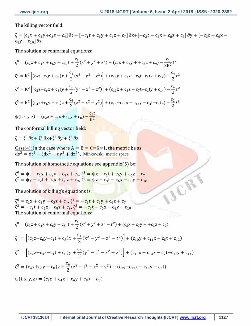
Case(3): In the case where A(t) = B(t) = C(t)=k, k is a constant the metric be as: ds2 = dt2 − k2(dx2 + dy2 + dz2)

The solution of homothetic equations see appendix(4) be:

ζ0 = 𝜓𝑡 + c1𝑥 + c2𝑦+c3𝑧 + 𝑐4, ζ1 = K2𝜓𝑥 − 𝑐1𝑡 + c5y + c6z + c7,

ζ2 = K2𝜓𝑦 − 𝑐2𝑡 − c5x + c8z + c9, , ζ3 = K2𝜓𝑧 − 𝑐3𝑡 − c6x − c8y + c10

The homothetic vector field:

ζ = [𝜓𝑡 + c1𝑥 + c2𝑦+c3𝑧 + 𝑐4] ∂t + [K2𝜓𝑥 − 𝑐1𝑡 + c5y + c6z + c7] ∂x+[K2𝜓𝑦 − 𝑐2𝑡 − c5x + c8z +c9] ∂y + [K2𝜓𝑧 − 𝑐3𝑡 − c6x − c8y + c10] ∂z

The solution of killing’s equations is:

ζ0 = c1𝑥 + c2𝑦+c3𝑧 + 𝑐4, ζ1 = −𝑐1𝑡 + c5y + c6z + c7,

ζ2 = −𝑐2𝑡 − c5x + c8z + c9, ζ3 = −𝑐3𝑡 − c6x − c8y + c10

www.ijcrt.org © 2018 IJCRT | Volume 6, Issue 2 April 2018 | ISSN: 2320-2882

IJCRT1813014 International Journal of Creative Research Thoughts (IJCRT) www.ijcrt.org 1127

The killing vector field:

ζ = [c1𝑥 + c2𝑦+c3𝑧 + 𝑐4] ∂t + [−𝑐1𝑡 + c5y + c6z + c7] ∂x+[−𝑐2𝑡 − c5x + c8z + c9] ∂y + [−𝑐3𝑡 − c6x −c8y + c10] ∂z

The solution of conformal equations:

ζ0 = (c2z + c4x + c6y + c8)𝑡 +c1

2(x2 + y2 + z2) + (c5x + c7y + +c3z + c9) −

c1

2K2𝑡2

ζ1 = K2 [(c2z+c6y + c8)𝑥 +c4

2(x2 − y2 − z2)] + (c10y + c3z − c5t−c1tx + c12) −

c4

2𝑡2

ζ2 = K2 [(c2z+c6x + c8)𝑦 +c6

2(y2 − x2 − z2)] + (c10x + c3z − c7t−c1ty + c14) −

c6

2𝑡2

ζ3 = K2 [(c4x+c6y + c8)𝑧 +c6

2(z2 − x2 − y2)] + (c15−c11x − c13y − c3t−c1tz) −

c2

2𝑡2

ψ(t, x, y, z) = (𝑐2𝑧 + c4x + c6y + c8) −𝑐1𝑡

K2

The conformal killing vector field:

ζ = ζ0 ∂t + ζ1 ∂x+ζ2 ∂y + ζ3 ∂z

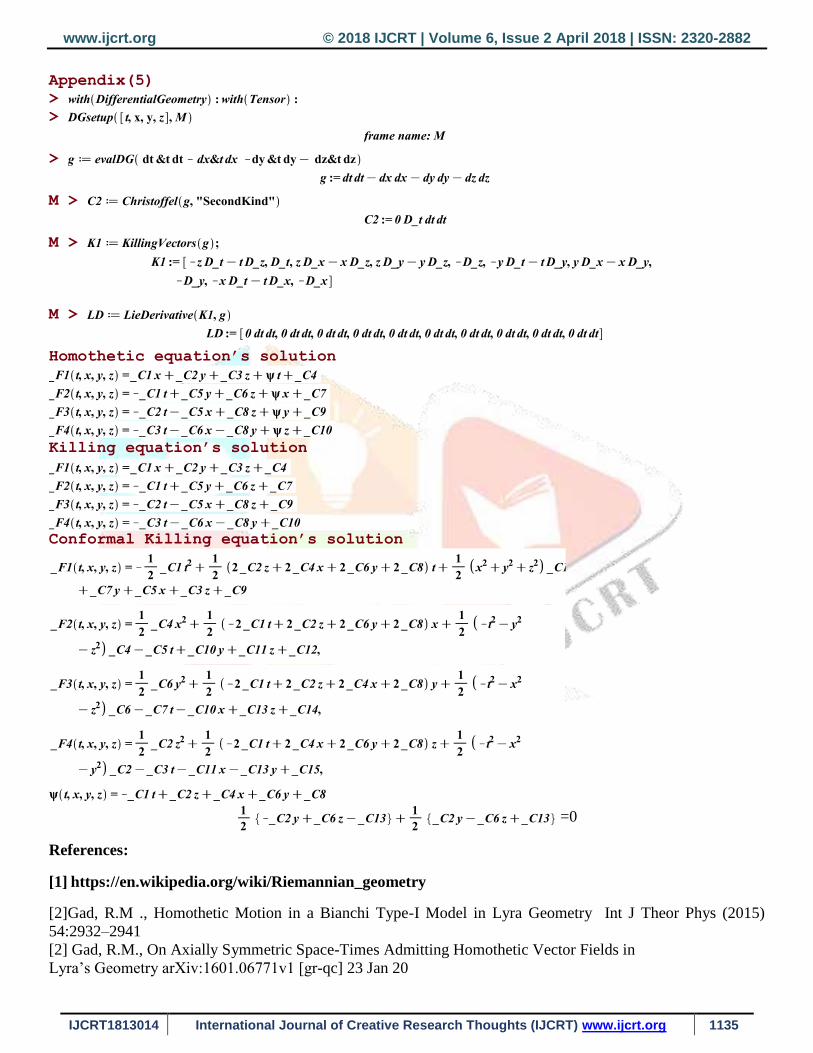
Case(4): In the case where A = B = C=K=1, the metric be as: ds2 = dt2 − (dx2 + dy2 + dz2), Minkowski metric space

The solution of homothetic equations see appendix(5) be:

ζ0 = ψt + c1x + c2y + c3z + c4, ζ1 = ψx − c1t + c6y + c6z + c7

ζ2 = ψy − c2t + c5x + c8z + c9, ζ3 = ψz − c3t − c6x − c8y + c10

The solution of killing’s equations is:

ζ0 = c1x + c2y + c3z + c4, ζ1 = −c1t + c6y + c6z + c7

ζ2 = −c2t + c5x + c8z + c9, ζ3 = −c3t − c6x − c8y + c10

The solution of conformal equations:

ζ0 = (c2z + c4x + c6y + c8)𝑡 +c1

2(x2 + y2 + z2 − 𝑡2) + (c5x + c7y + +c3z + c9)

ζ1 = [(c2z+c6y−c1t + c8)𝑥 +c4

2(x2 − y2 − z2 − 𝑡2)] + (c10y + c11z − c5t + c12)

ζ2 = [(c2z+c4x−c1t + c8)𝑦 +c6

2(y2 − t2 − x2 − z2)] + (c10x + c13z − c7t−c1ty + c14)

ζ3 = (c4x+c6y + c8)𝑧 +c6

2(z2 − t2 − x2 − y2) + (c15−c11x − c13y − c3t)

ψ(t, x, y, z) = (𝑐2𝑧 + c4x + c6y + c8) − 𝑐1𝑡

www.ijcrt.org © 2018 IJCRT | Volume 6, Issue 2 April 2018 | ISSN: 2320-2882

IJCRT1813014 International Journal of Creative Research Thoughts (IJCRT) www.ijcrt.org 1128

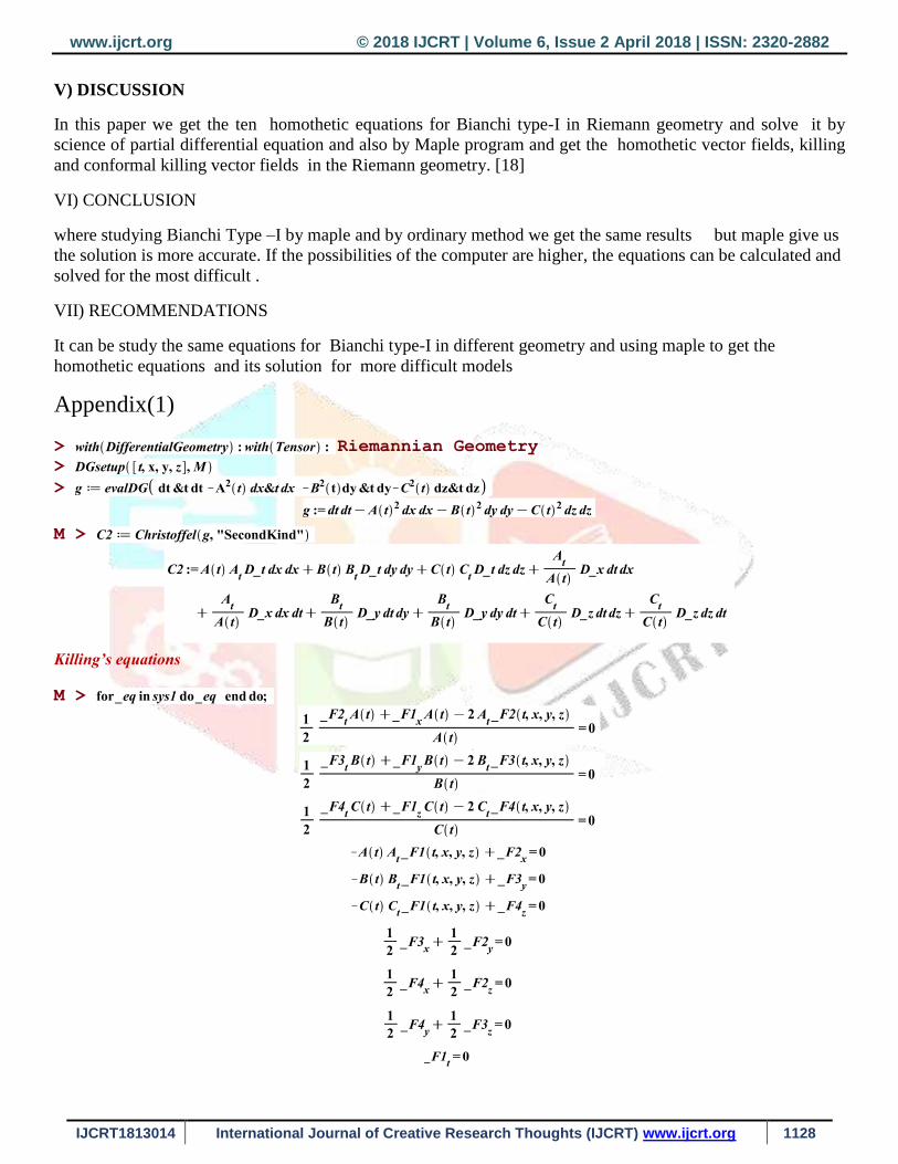
V) DISCUSSION

In this paper we get the ten homothetic equations for Bianchi type-I in Riemann geometry and solve it by

science of partial differential equation and also by Maple program and get the homothetic vector fields, killing

and conformal killing vector fields in the Riemann geometry. [18]

VI) CONCLUSION

where studying Bianchi Type –I by maple and by ordinary method we get the same results but maple give us

the solution is more accurate. If the possibilities of the computer are higher, the equations can be calculated and

solved for the most difficult .

VII) RECOMMENDATIONS

It can be study the same equations for Bianchi type-I in different geometry and using maple to get the

homothetic equations and its solution for more difficult models

Appendix(1)

> Riemannian Geometry >

>

M >

Killing’s equations

M >

www.ijcrt.org © 2018 IJCRT | Volume 6, Issue 2 April 2018 | ISSN: 2320-2882

IJCRT1813014 International Journal of Creative Research Thoughts (IJCRT) www.ijcrt.org 1129

Check the solution:

M >

M >

The homothetic equations in Riemannian geometry

www.ijcrt.org © 2018 IJCRT | Volume 6, Issue 2 April 2018 | ISSN: 2320-2882

IJCRT1813014 International Journal of Creative Research Thoughts (IJCRT) www.ijcrt.org 1130

M > ,

Appendix(2):

> Where A(t)=B(t)=C(t) >

>

Killing equations

M >

Solution of killig’s equations:

Homothetic equations

www.ijcrt.org © 2018 IJCRT | Volume 6, Issue 2 April 2018 | ISSN: 2320-2882

IJCRT1813014 International Journal of Creative Research Thoughts (IJCRT) www.ijcrt.org 1131

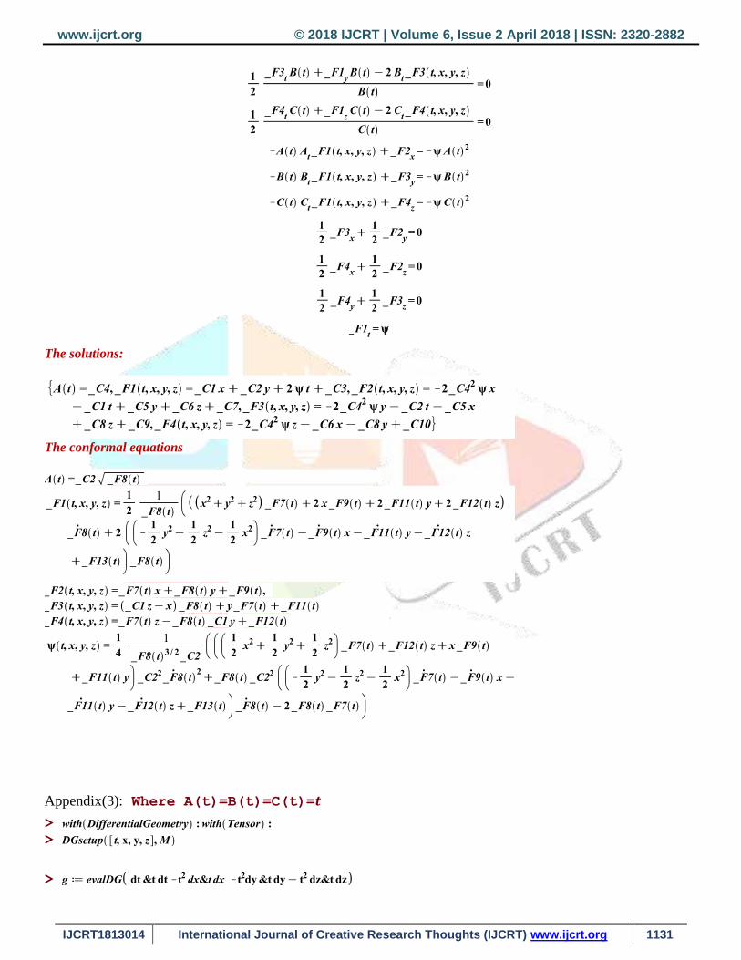
The solutions:

The conformal equations

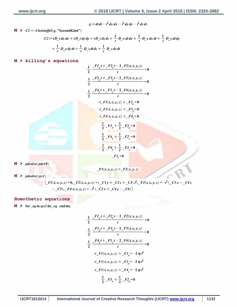
Appendix(3): Where A(t)=B(t)=C(t)=𝒕

>

>

>

www.ijcrt.org © 2018 IJCRT | Volume 6, Issue 2 April 2018 | ISSN: 2320-2882

IJCRT1813014 International Journal of Creative Research Thoughts (IJCRT) www.ijcrt.org 1132

M >

M > killing’s equations

M >

M >

Homothetic equations

M >

www.ijcrt.org © 2018 IJCRT | Volume 6, Issue 2 April 2018 | ISSN: 2320-2882

IJCRT1813014 International Journal of Creative Research Thoughts (IJCRT) www.ijcrt.org 1133

M >

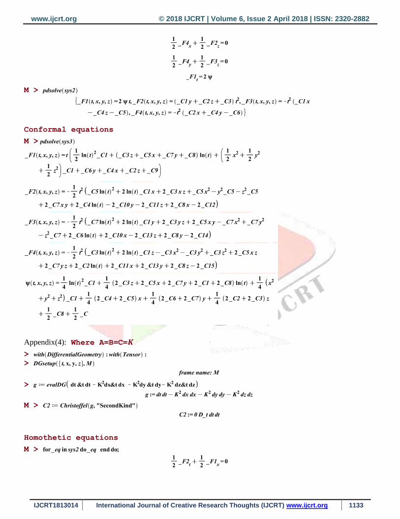
Conformal equations

M >

Appendix(4): Where A=B=C=𝑲

>

>

>

M >

Homothetic equations

M >

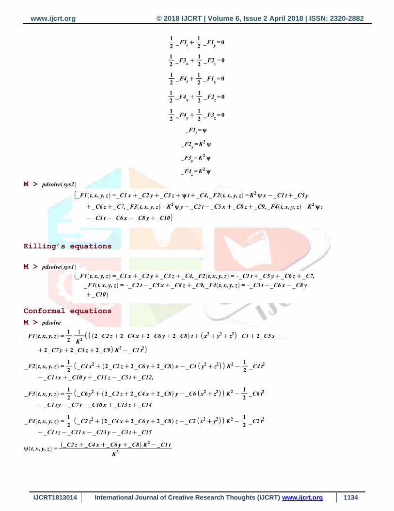
www.ijcrt.org © 2018 IJCRT | Volume 6, Issue 2 April 2018 | ISSN: 2320-2882

IJCRT1813014 International Journal of Creative Research Thoughts (IJCRT) www.ijcrt.org 1134

M >

Killing’s equations

M >

Conformal equations

M >

www.ijcrt.org © 2018 IJCRT | Volume 6, Issue 2 April 2018 | ISSN: 2320-2882

IJCRT1813014 International Journal of Creative Research Thoughts (IJCRT) www.ijcrt.org 1135

Appendix(5)

>

>

>

M >

M >

M >

Homothetic equation’s solution

Killing equation’s solution

Conformal Killing equation’s solution

=0

References:

[1] https://en.wikipedia.org/wiki/Riemannian_geometry

[2]Gad, R.M ., Homothetic Motion in a Bianchi Type-I Model in Lyra Geometry Int J Theor Phys (2015)

54:2932–2941

[2] Gad, R.M., On Axially Symmetric Space-Times Admitting Homothetic Vector Fields in

Lyra’s Geometry arXiv:1601.06771v1 [gr-qc] 23 Jan 20

www.ijcrt.org © 2018 IJCRT | Volume 6, Issue 2 April 2018 | ISSN: 2320-2882

IJCRT1813014 International Journal of Creative Research Thoughts (IJCRT) www.ijcrt.org 1136

[4] Nazrul Islam , Tensors and their applications Copyright © 2006, New Age International (P) Ltd.,

Publishers,

[5] Ragab M. Gad, “On Spherically Symmetric Perfect-Fluid Solutions Admitting Conformal Motions”IL

NUOVO CIMENTO B, 117B (2002), 533-547.

[6] Ragab M. Gad, "On spherically symmetric non-static space-times admitting homothetic motions", IL

NUOVO CIMENTO, 124, 61 (2009):

[7] Ragab M. Gad and M. M. Hassan, “On the Geometrical and Physical Properties of Spherically

Symmetric Non- Static Space-Times: Self-Similarity”, IL NUOVO CIMENTO B, 118B (2003), pp. 759–765.

[8]Hall G. S., Symmetries and Curvature Structure in General Relativity, World Scientific, (2004).

[9]Collins, M.E., Lang, J.M.: A class of self-similar perfect-fluid spacetimes, and a generalization Classical and

Quantum Gravity Volume 4, Number 1 (1987)

[10] F. Rahaman, homogeneous kantowski –sachs model in Lyra Geometry, Bulg. J. Phys. 29 (2002)

[11]Eardley DM. 1974. Phys. Rev. Lett. 33: 442 .

[12]Eardley DM. 1974. Commun. Math. Phys. 37: 287 .

[13] M. Sharif Nuovo Cimento B 116, 673 (2001)

[14] M. Sharif J. Math. phs. 45, 1518 (2004); ibid 1532; Astrophs. Space Sci 278, 447 (2001)

[15]Alicia M. Sintes, Infinite Kinematic Self-Similarity and Perfect Fluid Space-times, General Relativity and

Gravitation, Vol. 33, No. 10, October 2001

[16]Ravi & Lallan, Bianchi type-v cosmological models of the universe for bulk viscous fluid distribution in

general relativity: expressions for some observable quantities Romanian Reports in Physics, Vol.63,No. 2

p.587-605,2011

[17]Stephani H., Kramer D., MacCallum M. A. H., Hoenselears C. and Herlt E., Exact Solutions of

Einstein’s Field Equations, Cambridge University Press, (2003).

[18]M. Sharif J. Math. phs. 45, 1518 (2004); ibid 1532; Astrophs. Space Sci 278, 447 (2001)

[19] https://arxiv.org/abs/1503.02097

[20] El-Sabbagh , Moustafa ,EL- Homothetic Motion in a Bianchi Type –V Model in Lyra Geometry Journal

of natural sciences, life and applied sciences ,V1,51-65 December (2017)