Embed Size (px)
Citation preview

Effect on Different Economic Factors on NDP(National Domestic Product)
Department of Statistics
University Of Calcutta
Roll No:91/STS/131032
Reg No: A03-1112-0103-10
6 / 1 / 2 0 1 5
Subhodeep Mukherjee

Contents:
• Introduction & Motivation For The Project• Some Definitions Before The Start Of Analysis• Comparison Of percentage share of Different Economic Factors in two
years• Percentage Share of the factor incomes year wise:• Analysis:
Dickey-Fueller Test for the test of unit roots Fitting ARMA Model
Diagnostic Testing (for the Goodness Of fit):Ljung-Box Test
Fitting a GARCH Model Prediction
Comparison Of Contribution of Factor Incomes to NDP Percentage Share of the factor incomes year wise(the predicted values)
Findings from the predicted percentage shares:
• MULTIVARIATE TIME SERIES ANALYSIS:• Our Findings and Conclusions• Appendix• References

Introduction & Motivation For The Project
The global economic structure of India is changing from the post independence era. Though it mainly relies on Agriculture in the beginning , but nowadays it relies more on other economic factors. The main objective of my project is to see how the different factors incomes impact the Net Domestic Product of Our Country and also predict some future values. Also we will see that How much the factor incomes effect NDP in the future?
For this we have collected data on factor incomes.The different factor incomes are:
Agriculture ,Manufacturing ,forestry ,logging , mining &fishing, Construction ,Electricity ,gas & watersupply, Finance, Real Estate, Insurance & Business Services, Social & Personal Services, Trade ,Hotels ,Transport & Communication.

Some Definitions Before The Start Of Analysis
Before the start of the analysis we should know the meaning of the following terms:
GDP (Gross Domestic Product):
It is defined as an aggregate measure of production equal to the sum of the gross values added of all resident, institutional units engaged in production (plus any taxes, and minus any subsidies, on products not included in the value of their outputs).
It is measured in three different approaches:
Product Approach Income Approach Expenditure Approach
But we will use the Income Approach
Income Approach:
It is the sum of primary incomes distributed by resident producer units .It is measured as
GDP = compensation of employees + gross operating surplus + gross mixed income+ taxes less subsidies on production and imports
Compensation of employees (COE) measures the total remuneration to employees for work done. It includes wages and salaries, as well as employer contributions to social security and other such programs.
Gross operating surplus (GOS) is the surplus due to owners of incorporated businesses. Often called profits, although only a subset of total costs are subtracted from gross output to calculate GOS.
Gross mixed income (GMI) is the same measure as GOS, but for unincorporated businesses. This often includes most small businesses.
The sum of COE, GOS and GMI is called total factor income. Adding taxes less subsidies on production and imports converts GDP at factor cost to GDP(I).
Total factor income is also sometimes expressed as:
Total factor income = employee compensation + corporate profits + proprietor's income + rental income + net interest

NDP:
The full form of NDP is National Domestic Product. It is the gross domestic product (GDP) minus depreciation on a country's capital goods.
Net domestic product accounts for capital that has been consumed over the year in the form of housing, vehicle, or machinery deterioration. The depreciation accounted for is often referred to as "capital consumption allowance" and represents the amount of capital that would be needed to replace those depreciated assets.
If the country is not able to replace the capital stock lost through depreciation, then GDP will fall. In addition, a growing gap between GDP and NDP indicates increasing obsolescence of capital goods, while a narrowing gap means that the condition of capital stock in the country is improving. It reduces the value of capital that is why it is separated from GDP to get NDP.

Comparison Of percentage share of Different Economic Factors in two years
For this we draw 2 pie diagrams for two years. These 2 diagrams are given below:
First the pie diagram for the factor incomes percentage shares for the year 1980
Agriculture36%
forestry and log-ging and fishing
4%
Mining & Quarrying
1%
Manufacturing
17%
Electricity, gas and
water supply
1%
Construc-tion5%
Trade,Hotels,Transport&Communica-
tion16%
Finance,
Insurance, Real Es-tate &
Business Services
8%
Social & Personal Services
1980
In this diagram we can see the impact of Agriculture and Manufacturing Industry is more than other factors

Second the pie diagram for the factor incomes percentage shares for the year 2013.
In the given diagram we can see the impact of Other factors is more than Agriculture and Manufacturing Industry.
Agriculture14%
forestry and logging and fishing
2%
Mining & Quarrying
2%
Manufactur-ing
13%
Electricity, gas and
water sup-ply2%
Construc-tion8%
Trade,Hotels,Transport&Communicati
on24%
Finance,
Insurance, Real Estate & Business
Services19%
Social & Personal Services
2013

Percentage Share of the factor incomes year wise:
1980 1985 1990 1995 2000 2005 2010
1525
35
time
Agricul
ture %
share
1980 1985 1990 1995 2000 2005 2010
1.02.0
3.0
time
Forestr
y & log
ging &fis
hing %
share
1980 1985 1990 1995 2000 2005 2010
1.52.0
2.5
time
Mining
& Quar
rying %
share
1980 1985 1990 1995 2000 2005 2010
1315
17
time
Manufac
turing %
share
1980 1985 1990 1995 2000 2005 2010
1.01.5
2.02.5
timeElectrici
ty,gas a
nd water
supply
% shar
e
1980 1985 1990 1995 2000 2005 2010
5.06.0
7.08.0
time
Constru
ction %
share
1980 1985 1990 1995 2000 2005 2010
1418
22
time
Trade,H
otels,T
ranspo
rt and C
ommunic
ation %
share
1980 1985 1990 1995 2000 2005 2010
812
16
time
Banking
,Financ
e,Insur
ance,R
eal Est
ate and
Busine
ss Serv
ices %
share
1980 1985 1990 1995 2000 2005 2010
1113
1517
time
Public.a
dminist
ration.an
d.Defen
ce,socia
l and pe
rsonal
shares
% sha
re

From the diagram given above we have the following observations:
Here the agriculture share decreases and falls steeply from 1996 till 2007 after wards becomes stable
The Forestry, logging and fishing share decreases suddenly after 2000-2003 and after that again rises.
In case of Mining & Quarrying the share falls and rises quite frequently but it has an increasing trend.
The manufacturing industry has steep rise and falls in the end finally falls steeply after 2007.
In case of Electricity, gas and water supply we see an increasing trend till 2000 and a decreasing trend after 2000.
In case of Construction the percentage share curve has a steep rise so we can say that construction industry has an increasing impact on Indian Economy .
Though there is a steep depression from the years 1990-2000 ,the trade,hotels,transport and communication industry has recovered from this phase and now has a great position.
The Banking,Finance,Insurance,Real Estate and Business Services percentage share here increases and we can interpret it by saying people are using banks and are interested in financial services which is a very good sign.
In case of public administration,defence,socil and personal services also we can see an upward trend with a boom in the year 2000.

Analysis:
The Analysis will be mainly Time Series Analysis which will be done in the following way:
Next we shall follow the steps given above.
Note: The prediction will be 5 years because government usually form 5 years plan .
Step-1Test for
stationarity using Augmented
Dickey Fueller Test
Removing Stationarity:We
shall remove stationarity by
differencing
Step-2Fitting ARMA
Model: We Shall Fit ARMA model on the data and
check the goodness of fit by AIC.
We shall check for the volatility of the residuals
Step-3 Check For Volatility
If Volatility presents we shall
go for trhe GARCH model
Step-4 PredictionUsing the given
time series predict for the next 5 years.

Step-1:
Dickey-Fueller Test for the test of unit roots:
This test is used to test whether there is any unit roots .The presence of unit roots doesn’t make the series stationary.As the result the trend component involved in the dataset doesn’t gets removed.
Performing Dickey-Fueller test on our dataset we have the following results:
Variables ADF Test p-Values
No of differencing
ADF Test p-Values after differencing
Agriculture 0.9821 3 0.03591
Forestry,logging &fishing 0.9677 3 <0.01
Mining & Quarrying >0.99 2 0.02759
Manufacturing >0.99 2 0.04569
Electricity,gas and water supply >0.99 3 0.01219
Construction >0.99 4 0.01296
Trade,Hotels,Transport and Communication
>0.99 2 <0.01
Banking ,Finance,Insurance,Real Estate and Business Services
>0.99 3 0.0125
Public.administration.and.Defence,social and personal Services
>0.99 3 <0.01
Net domestic Product >0.99 3 <0.01
So all the variables have to be differenced the given number of times to get stationary time series.

Step-2:
Fitting ARMA Model:
Consider a given time series given over time t
Y t=μt+X t
Where X t evolves over time.
Where Y tis the observed value of the variable,
μt is the part of the time series variable explained by the mean part with E(X t)=0
X t is the residual part .If the process has volatility X t becomes ϵ t∗σ t and σ t has a specific form whereas if X t = ϵ t (in both cases ϵ t is a White Noise process).Thus in the former case we have to go for ARCH or GARCH model.
μt is modelled using the ARMA ,ARIMA or SARIMA to get μ̂ .
For the model we take the following notations:
Y 1 t:Incomes from Agriculture at time t
Y 2 t:Incomes from Forestry & logging &fishing at time t
Y 3 t: Incomes from Mining & Quarrying at time t
Y 4 t: Incomes from Manufacturing at time t
Y 5 t: Incomes from Electricity,gas and water supply at time t
Y 6 t: Incomes from Construction at time t
Y 7 t: Incomes from Trade,Hotels,Transport and Communication at time t
Y 8 t: Incomes from Banking ,Finance,Insurance,Real Estate and Business Services at time t
Y 9 t: Incomes from Public administration and Defence,social and personal services at time t
Y 10 t:National Domestic Product values at time t

The ARMA model is given as :∅ (B)Y t=φ (B)X t,where ∅ (B) is the AR component and φ (B) is the MA Component of a Time Series.
For Agriculture:
ARMA(2,2) is the best model for the Agriculture stationary data with AIC= 742.01.Thus the model is given below:
Y 1 t=1.8225¿Y 1(t−1)−0.1083∗Y 1 ( t−2)−0.6101∗Y 1 (t−3)−0.7449∗Y 1 ( t−4 )+0.6408∗Y 1( t−5 )+X1 t+0.3175∗X1 (t−1)+0.5525∗X1(t−2 )
For Forestry ,Logging & Fishing :
ARMA(3,0) is the best model for the Forestry , Logging & Fishing stationary data with AIC= 657.04.Thus the model is given below:
Y 2 t=1.9956 ¿Y 2(t−1)−0.8931∗Y 2 ( t−2)−0.0642∗Y 2 (t−3)+0.5952∗Y 2 (t−4)+1.4034∗Y 2 ( t−5)+0.7699∗Y 2 (t−6)+X2 t
For Mining & Quarrying :
ARMA(0,1) is the best model for the Mining & Quarrying stationary data with AIC= 674.55.Thus the model is given below:
Y 3 t=2¿Y 3(t−1)−Y 3 (t−2 )+ϵ 3t+0.6732∗X3(t−1 )
For Manufacturing :
ARMA(0,0) is the best model for the Manufacturing stationary data with AIC=756.08.Thus the model is given below:
Y 4 t=2¿Y 4 (t−1)−Y 4 (t−2)+X 4 t
For Electricity,gas and water supply :
ARMA(1,1) is the best model for the Electricity,gas and water supply stationary data with AIC= 652.81.Thus the model is given below:
Y 5 t=2.3793¿Y 5(t−1)−1.1379∗Y 5( t−2 )−0.8621∗Y 5 ( t−3 )+0.6207∗Y 5 ( t−4 )+X5 t+0.8663∗X5(t−1)
For Construction :
ARMA(0,2) is the best model for the Construction stationary data with AIC= 682.7.Thus the model is given below:
Y 6 t=4 ¿Y 6(t−1)−6∗Y 6 (t−2)+4∗Y 6 ( t−3 )−Y 6 (t−4 )+X6 t+1.9651∗X6 (t−1)−0.9842∗X6 (t−2)

For Trade,Hotels,Transport and Communication :
ARMA(0,0) is the best model for the Trade,Hotels,Transport and Communication stationary data with AIC= 769.83.Thus the model is given below:
Y 7 t=2¿Y 7(t−1)−Y 7 (t−2)+X7 t
For Banking ,Finance,Insurance,Real Estate and Business Services :
ARMA(1,1) is the best model for the Banking ,Finance,Insurance,Real Estate and Business Services stationary data with AIC= 713.53.Thus the model is given below:
Y 8 t=2.4058 ¿Y 8(t−1)−1.2174∗Y 8 ( t−2)−0.7826∗Y 8 (t−3 )+0.5942∗Y 8 ( t−4 )+X8 t−0.6281∗X8 (t−1)
For Public administration and Defence,social and personal services :
ARMA(0,1) is the best model for the Public administration and Defence,social and personal services stationary data with AIC= 714.43.Thus the model is given below:
Y 9 t=3¿Y 9(t−1 )−3∗Y 9 (t−2)+Y 9 (t−3)+X9 t+0.9358∗X9(t−1 )
Here the models are chosen by minimum AIC.

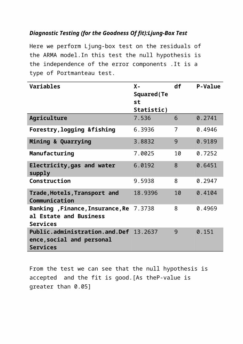
Diagnostic Testing (for the Goodness Of fit):Ljung-Box Test
Here we perform Ljung-box test on the residuals of the ARMA model.In this test the null hypothesis is the independence of the error components .It is a type of Portmanteau test.
Variables X-Squared(Test Statistic)
df P-Value
Agriculture 7.536 6 0.2741
Forestry,logging &fishing 6.3936 7 0.4946
Mining & Quarrying 3.8832 9 0.9189
Manufacturing 7.0025 10 0.7252
Electricity,gas and water supply 6.0192 8 0.6451
Construction 9.5938 8 0.2947
Trade,Hotels,Transport and Communication
18.9396 10 0.4104
Banking ,Finance,Insurance,Real Estate and Business Services
7.3738 8 0.4969
Public.administration.and.Defence,social and personal Services
13.2637 9 0.151
From the test we can see that the null hypothesis is accepted and the fit is good.[As theP-value is greater than 0.05]

Now the fitted values are given by the following plot:
time
Agricult
ure
1980 1985 1990 1995 2000 2005 2010
0600
000140
0000
time
Forestr
y & logg
ing &fis
hing
1980 1985 1990 1995 2000 2005 2010
0100
000200
000
time
Mining
& Quarr
ying
1980 1985 1990 1995 2000 2005 2010
0100
000
time
Manufac
turing
1980 1985 1990 1995 2000 2005 2010
0600
000140
0000
time
Electrici
ty,gas a
nd water
supply
1980 1985 1990 1995 2000 2005 2010
0100
000200
000
time
Constru
ction
1980 1985 1990 1995 2000 2005 2010
0e+00
4e+05
8e+05
time
Trade,H
otels,Tr
ansport
and Co
mmunic
ation
1980 1985 1990 1995 2000 2005 2010
0100
0000
250000
0
time
Banking
,Financ
e,Insura
nce,Re
al Estat
e and Bu
siness S
ervices
1980 1985 1990 1995 2000 2005 2010
0100
0000
time
Public a
dminist
ration an
d Defen
ce,socia
l and pe
rsonal s
ervices
1980 1985 1990 1995 2000 2005 2010
0100
0000
Here some points are missing the line

So now we have a residual plot after fitting of the ARMA model.
time
Agricul
ture
1980 1985 1990 1995 2000 2005 2010
-50000
0500
00
time
Forest
ry & log
ging &fi
shing
1980 1985 1990 1995 2000 2005 2010
-10000
20000
time
Mining
& Quar
rying
1980 1985 1990 1995 2000 2005 2010
-20000
0200
00
time
Manuf
acturin
g
1980 1985 1990 1995 2000 2005 2010
-50000
50000
time
Electri
city,ga
s and
water s
upply
1980 1985 1990 1995 2000 2005 2010
-20000
0200
00
time
Constru
ction
1980 1985 1990 1995 2000 2005 2010
-60000
0400
00
time
Trade,
Hotels,
Transp
ort and
Comm
unicatio
n
1980 1985 1990 1995 2000 2005 2010
-50000
50000
time
Banking
,Finan
ce,Ins
urance
,Real E
state a
nd Bus
iness S
ervices
1980 1985 1990 1995 2000 2005 2010
-40000
0400
00
time
Public a
dminis
tration
and De
fence,
social a
nd per
sonal s
ervices
1980 1985 1990 1995 2000 2005 2010
-60000
0400
00
Here as the some values are too high or too low we can say that there is volatility in the data. So we have to fit the Garch Model on the data.

Step-3:
Fitting a GARCH Model:
The Garch model is given as X t=σ t∗ϵ t where (σ t❑)2=∑
i=0
p
δi∗X t−i+∑i=1
q
θ i∗(σ t−i❑ )2
For Agriculture:
GARCH(1,1) is the best model for the Agriculture stationary data . Thus the model is given below:
(σ 1t❑)2=774273200+0.3570242∗(X1 (t−1) )2+0.1311034∗(σ1 ( t−1) )2
For Forestry ,Logging & Fishing :
GARCH(1,1) is the best model for the Forestry ,Logging & Fishing stationary data . Thus the model is given below:
(σ 2t❑)2=55011800+0.2145423∗(X2 (t−1 ))2+0.0000003335437∗(σ2 ( t−1) )2
For Mining & Quarrying :
GARCH(1,1) is the best model for the Mining & Quarrying stationary data . Thus the model is given below:
(σ 3 t❑ )2=62556220+1.516188∗(X3 ( t−1) )2+0.004745028∗(σ3 (t−1) )2
For Manufacturing :
GARCH(1,1) is the best model for the Manufacturing stationary data . Thus the model is given below:
(σ 4 t❑ )2=8755697 00+0.1827009∗(X 4 (t−1 ) )2+0.000001794393∗(σ 4 (t−1 ) )2
For Electricity,gas and water supply :
GARCH(1,1) is the best model for the Electricity,gas and water supply stationary data . Thus the model is given below:
(σ 5 t❑ )2=507628800+1.048942∗(X5 (t−1) )2+0.0000003637639∗(σ 5 (t−1 ))2
For Construction :

GARCH(1,1) is the best model for the Construction stationary data . Thus the model is given below:
(σ 6 t❑ )2=181192800+0.2139037∗(X6 (t−1) )2+0.000003040251∗(σ 6 (t−1 ) )2
For Trade,Hotels,Transport and Communication :
GARCH(1,1) is the best model for the Trade,Hotels,Transport and Communication stationary data . Thus the model is given below:
(σ 7 t❑ )2=1320244000+0.005∗(X7 ( t−1 ))2+0.005∗(σ7 (t−1) )2
For Banking ,Finance,Insurance,Real Estate and Business Services :
GARCH(1,1) is the best model for the Banking ,Finance,Insurance,Real Estate and Business Services stationary data . Thus the model is given below:
(σ 8 t❑ )2=362260400+1.026698∗(X 8( t−1 ))2+0.000001418799∗(σ8 (t−1) )2
For Public administration and Defence,social and personal services :
GARCH(1,1) is the best model for the Public administration and Defence,social and personal services stationary data . Thus the model is given below:
(σ 9 t❑ )2=404505700+1.048756∗(X9 (t−1) )2+0.000002044029∗(σ 9 (t−1 ) )2

Now we want to see the effect of all the covariates at the same time.So we will use the multivariate analogue of the usual Time Series i.e. a VAR Model.
MULTIVARIATE TIME SERIES ANALYSIS:
A multivariate analogue to our current analysis is to use the VAR model.The usual Vector Autoregressive model (VAR) of order p is given below:
X t=A1∗X ( t−1)+A2∗X ( t−2)+…+A p∗X (t−p )+∈t
Where X t is the vector of time series variables and Ai’s are coefficient matrices.
A Second form of the model is the Error Correction Model which is given below:
∆ X t=δ+π∗X (t−1)+A1 '∗∆ X ( t−1 )+A2 '∗∆ X (t−2 )+…+Ap '∗∆ X (t−p )+∈t
Where π=G*H' and H' is the cointegrating matrix
For fitting the VAR model we have to see whether the given data is cointegrated to test for stationarity of the given data.
So we perform Johansen’s Test which gives the following results:
Eigenvalues (lambda):
9.982438e-01 9.872533e-01 9.817916e-01 9.540891e-01 8.557612e-01
8.486086e-01 5.645060e-01 4.441629e-01 7.448209e-02 -2.081668e-16
Values of test statistic and critical values of test:
test 10pct 5pct 1pct
r<=8 | 2.48 10.49 12.25 16.26
r<=7 | 18.79 16.85 18.96 23.65
r<=6 | 26.6 23.11 25.54 30.34
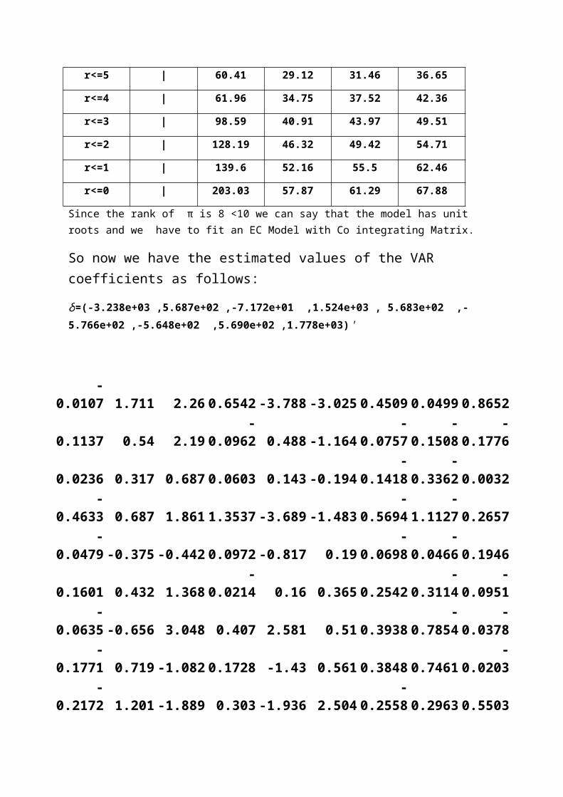
r<=5 | 60.41 29.12 31.46 36.65
r<=4 | 61.96 34.75 37.52 42.36
r<=3 | 98.59 40.91 43.97 49.51
r<=2 | 128.19 46.32 49.42 54.71
r<=1 | 139.6 52.16 55.5 62.46
r<=0 | 203.03 57.87 61.29 67.88
Since the rank of π is 8 <10 we can say that the model has unit roots and we have to fit an EC Model with Co integrating Matrix.
So now we have the estimated values of the VAR coefficients as follows:
δ=(-3.238e+03 ,5.687e+02 ,-7.172e+01 ,1.524e+03 , 5.683e+02 ,-5.766e+02 ,-
5.648e+02 ,5.690e+02 ,1.778e+03)'
-0.0107 1.711 2.26 0.6542 -3.788 -3.025 0.4509 0.0499 0.8652
0.1137 0.54 2.19 -0.0962 0.488 -1.164 -0.0757 -0.1508 -0.1776
0.0236 0.317 0.687 0.0603 0.143 -0.194 -0.1418 -0.3362 0.0032
-0.4633 0.687 1.861 1.3537 -3.689 -1.483 -0.5694 -1.1127 0.2657
-0.0479 -0.375 -0.442 0.0972 -0.817 0.19 -0.0698 -0.0466 0.1946
0.1601 0.432 1.368 -0.0214 0.16 0.365 0.2542 -0.3114 -0.0951
-0.0635 -0.656 3.048 0.407 2.581 0.51 0.3938 -0.7854 -0.0378
-0.1771 0.719 -1.082 0.1728 -1.43 0.561 0.3848 0.7461 -0.0203
-0.2172 1.201 -1.889 0.303 -1.936 2.504 -0.2558 0.2963 0.5503A1'=¿
A2'=¿
1.4186 0.00348 5.302 -0.6288 -5.11 0.4663 -0.1388 -0.8322 -0.0128-0.0707 -0.11726 1.016 0.2962 -0.804 1.2232 0.1243 -0.1032 -0.1797
-0.0674-
0.03084 0.624 -0.1106 1.088 0.4343 0.0926 -0.0119 0.26390.6912 0.74337 7.535 -1.4054 5.047 2.0921 0.403 -0.581 0.7703
0.1196-
0.02824 0.322 -0.207 1.006 0.0885 0.0641 -0.0165 -0.01370.0243 0.23226 -0.881 -0.2746 0.651 0.6107 -0.0236 0.0805 -0.0758
-0.4014 -0.3115 -1.818 0.0164 -0.121 0.1251 0.1219 0.6366 0.6204
0.5338-
1.25299 -1.675 -0.5942 -2.267 0.8548 -0.2309 0.1949 0.3410.3126 -2.0733 -2.391 -0.2038 0.952 -0.4908 0.0262 -0.2423 0.6013

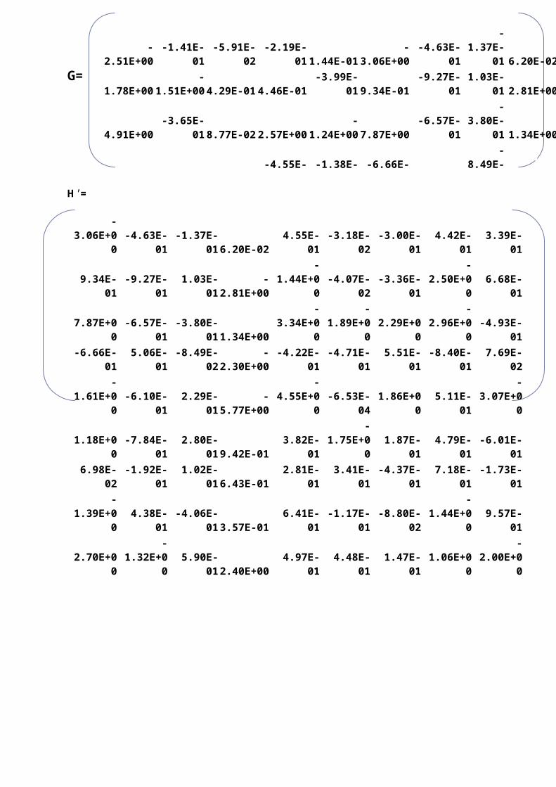
G=
H'=
-3.06E+00 -4.63E-01 -1.37E-01 6.20E-02 4.55E-01 -3.18E-02 -3.00E-01 4.42E-01 3.39E-01
9.34E-01 -9.27E-01 1.03E-01 -2.81E+00 -1.44E+00 -4.07E-02 -3.36E-01 -2.50E+00 6.68E-01
7.87E+00 -6.57E-01 -3.80E-01 1.34E+00 -3.34E+00 -1.89E+00 2.29E+00 -2.96E+00 -4.93E-01
-6.66E-01 5.06E-01 -8.49E-02 -2.30E+00 -4.22E-01 -4.71E-01 5.51E-01 -8.40E-01 7.69E-02
-1.61E+00 -6.10E-01 2.29E-01 -5.77E+00 -4.55E+00 -6.53E-04 1.86E+00 5.11E-01 -3.07E+00
1.18E+00 -7.84E-01 2.80E-01 9.42E-01 3.82E-01 -1.75E+00 1.87E-01 4.79E-01 -6.01E-01
6.98E-02 -1.92E-01 1.02E-01 6.43E-01 2.81E-01 3.41E-01 -4.37E-01 7.18E-01 -1.73E-01
-1.39E+00 4.38E-01 -4.06E-01 3.57E-01 6.41E-01 -1.17E-01 -8.80E-02 -1.44E+00 9.57E-01
2.70E+00 -1.32E+00 5.90E-01 2.40E+00 4.97E-01 4.48E-01 1.47E-01 1.06E+00 -2.00E+00
-2.51E+00 -1.41E-01 -5.91E-02 -2.19E-01 1.44E-01 -3.06E+00 -4.63E-01 -1.37E-01 6.20E-02
1.78E+00 -1.51E+00 4.29E-01 4.46E-01 -3.99E-01 9.34E-01 -9.27E-01 1.03E-01 -2.81E+00
4.91E+00 -3.65E-01 8.77E-02 2.57E+00 -1.24E+00 7.87E+00 -6.57E-01 -3.80E-01 1.34E+00
5.72E-01 1.07E-01 1.63E-01 -4.55E-01 -1.38E-01 -6.66E-01 5.06E-01 -8.49E-02 -2.30E+00
-1.83E+00 3.25E-01 -2.58E-01 -4.07E+00 -2.66E+00 -1.61E+00 -6.10E-01 2.29E-01 -5.77E+00
2.94E-01 -5.96E-01 2.59E-02 1.27E-01 1.49E-01 1.18E+00 -7.84E-01 2.80E-01 9.42E-01
-3.33E-01 -2.91E-02 -6.25E-02 3.49E-01 4.48E-01 6.98E-02 -1.92E-01 1.02E-01 6.43E-01
-5.77E-01 2.52E-01 -2.91E-01 2.40E-01 4.69E-01 -1.39E+00 4.38E-01 -4.06E-01 3.57E-01
1.06E+00 -8.06E-01 8.45E-02 8.39E-01 3.29E-01 2.70E+00 -1.32E+00 5.90E-01 2.40E+00

Step-4:
Prediction
Here we have a five year prediction based on the time series model that we have obtained. Here we obtained predicted values from the ARMA model and also predicted values from the GARCH model and add both the values. These values are given below:
2014 2015 2016 2017 2018
Agriculture 1593810 1745342 1907452 2092458 2263180
Forestry, Logging & Fishing 222161.1 231791.4 227308.5 228772.1
228979.8
Minning & Qyarrying 233073.7 243495.3 253917 264338.6
274760.3
Manufacturing 1379171 1408303 1437435 1466567 1495699
Trade, Hotels ,Transport & Communication 2695120 2880332 3065544 3250756 3435968
Public administration and Defence ,social and personal services
1932909 2151252 2378487 2614613 2859632
Electricity, gas and water supply 239603.8 287786.8 334569.2 388037.9
443173.5
Construction 882073.2 950550.6 1023497 1100547 1181333
Banking ,Finance , Insurance ,Real Estate and Business Services
2271865 2659905 3076458 3537654 4033909

Comparison Of Contribution of Factor Incomes to NDP
For this we draw 2 pie diagrams for two years. These 2 diagrams are given below:
First the pie diagram for the factor incomes percentage shares for the year 2014.
Agriculture14% Forestry,Log
ging & Fish-ing2%
Minning &Qyarrying
2%
Manufactur-ing12%
Trade,Hotels,Transport & Commu-
nication24%
Public.ad-ministra-
tion.and.De-fence,social
and per-sonal ser-
vices17%
Electricity,gas and wa-ter supply
2%
Construction8%
Banking ,Finance,Insurance,Real Es-
tate and Business Services
20%
Factor Incomes in 2014
The predicted value also shows that the effect of agriculture becomes insignificant

Second the pie diagram for the factor incomes percentage shares for the year 2013.
Agriculture14% Forestry,Lo
gging & Fishing
1%
Minning &Qyarrying
2%
Manufactur-ing9%
Trade,Hotels,Transport & Commu-
nication21%
Public.ad-ministra-
tion.and.Defence,social
and per-sonal ser-
vices18%
Electricity,gas and wa-ter supply
3%
Construc-tion7%
Banking ,Finance,Insurance,Real Estate and Business Services
25%
Factor Incomes on 2018
The other factors are rising but still very slowly

Percentage Share of the factor incomes year wise(the predicted values):
The percentage share of the predicted factor incomes on the NDP is given below:
2014 2015 2016 2017 2018
13.90
13.94
13.98
time
Agricul
ture %
share
2014 2015 2016 2017 2018
1.41.6
1.8
time
Forest
ry & log
ging &fi
shing %
share
2014 2015 2016 2017 2018
1.70
1.85
2.00
time
Mining
& Quar
rying %
share
2014 2015 2016 2017 2018
9.510.
511.
5
time
Manuf
acturin
g % sh
are
2014 2015 2016 2017 2018
2.12.3
2.52.7
timeElectri
city,ga
s and
water s
upply %
share
2014 2015 2016 2017 2018
7.37.5
7.7
time
Constru
ction %
share
2014 2015 2016 2017 2018
21.5
22.5
23.5
time
Trade,
Hotels,
Transp
ort and
Comm
unicatio
n % sh
are
2014 2015 2016 2017 2018
2022
24
time
Banking
,Finan
ce,Ins
urance
,Real E
state a
nd Bus
iness S
ervices
% sha
re
2014 2015 2016 2017 2018
17.0
17.4
time
Public.a
dminis
tration.
and.De
fence,
social a
nd per
sonal s
hares
% shar
e

Findings from the predicted percentage shares:
• We can see that the share in the Agriculture decreases till 2015 ,rises from there and attains maximum in 2017 after which it again decreases.
• We see that Mining ,Forestry ,Manufacturing , Construction ,Trade & Hotels & Transport industry have a decreasing percentage shares and the government should look upon it in future
• We also find out that Financial Services and Electricity, Gas and water supply has an increasing percentage share and government should invest upon these factors as they provide them more incomes.

Our Findings and Conclusions
Our findings and conclusions on the given project are abridged below:
• Here we have data on factor incomes like Agriculture , Forestry & logging & fishing , Mining & Quarrying ,Manufacturing Electricity , gas and water supply ,Construction ,Trade,Hotels,Transport ,Banking ,Finance ,Insurance , Real Estate and Business Services Public administration and Defence,social and personal services and we have to study its effects on NDP and see how these are effecting NDP in future
• Here we see though Agriculture was the main determinant of Income at the first few years but later we find that other factors have more effect at the succeeding years and these play important roles in future.
• We see that Public administration and Defence , social and personal services , Banking , Finance , Insurance, Real Estate and Business Services, Construction ,Mining & Quarrying , Electricity , gas and water supply has an increasing trend though they are harmonic rising in some years and falling in some years
• We see the remaining factors have a decreasing percentage share of incomes.
• We have fitted ARMA Models on the entire data see that the fitting is good except for some points
• We have tested for Volatility factor and find that we have to fit GARCH Model on the data
• Here the most appropriate model is the GARCH (1,1) model and see that the residuals after fitting is not volatile
• We have used Augmented Dickey Fuller test before ARMA fitting to remove trend component by finding the no of unit roots, Portmanteau tests for diagnostic checking (goodness of fit of the ARMA model),Lagrange's test for the volatility checking.
• In case of ADF test we found the presence of unit roots in all the covariates and have to difference to remove trend .
• We have also fitted a Multivariate model to see the effects of the covariates at the same time on different years. Since Johansen’s Test suggests the presence of cointegrating effects we used Error Correction Model form of the usual VAR model having cointegrated effects(i.e Cointegrating matrix)
• Now we get predictions from the fitted model and can infer that under the continuing conditions the share in the Agriculture decreases till 2015 ,rises from there and attains maximum in 2017 after which it again decreases. Mining ,Forestry ,Manufacturing , Construction ,Trade & Hotels & Transport industry have a decreasing percentage shares and Financial Services and Electricity, Gas and water supply has an increasing percentage share.

Appendix:
1.Dickey-Fueller Test:
This test is used to see whether there is any unit root in the process i.e. whether the process is stationary or not.
The general regression equation which incorporates a constant and a linear trend is used and the t-statistic for a first order autoregressive coefficient equals one is computed. The number of lags used in the regression is k. The default value of trunc((length(x)-1)^(1/3)) corresponds to the suggested upper bound on the rate at which the number of lags, k, should be made to grow with the sample size for the general ARMA(p,q) setup. Note that for k equals zero the standard Dickey-Fuller test is computed. The p-values are interpolated from Table 4.2, p. 103 of Banerjee et al. (1993). If the computed statistic is outside the table of critical values, then a warning message is generated.
Let for an AR(1) process, Xt=α*Xt-1+εt, εt ~WN(0,σ2)
Null hypothesis,H0:| α |=1 vs H1:| α |<1
α̂ =∑t=1
n
X t X t−1/∑t=2
n
X t−12 is the ols estimator of α.
Usual test statistic: t= α̂-1/se(α̂)
Unfortunately , t, under H0,do not follow the usual t-distribution.
Note: Under H1,√n*(α̂-α)~N(0,σ2/ ∑t=2
n
X t−12 ¿
Under H0, n*(α̂-α) = 12 w (1 )−1
∫0
1
w ( t )dt , w(t) is a standard Brownian Motion
The AR(1) process given above can be written as
ΔXt =(α-1)Xt-1+εt =δXt-1+ εt
In this case it is enough to test that H0: δ=0.Therefore t=δ̂/se(δ̂).
In general for an AR(p) process we use Augmented Dickey Fueller test where
Xt=α1*Xt-1+….+αp*Xt-p+εt

For DF test of a unit root model is given as
ΔXt=δXt-1+C1 ΔXt-1 +….+Cp-1 ΔXt-p+εt where δ=∑i=1
p
αi-1
We have to test for H0: δ=0
2.Ljung-BoxTest :
It is a portmanteau test used for the diagnostic testing i.e. goodness of fit of an ARMA model.The test statisticis given as
Qp*=n(n+2) ∑
h=1
h∗¿ ρ̂ (h )r/(n−h)¿
¿~asympχh∗−( p+q)2
References:
Theory Sources:
• Economics: Paul & Samuelson , William D Nordhaus
• Chris Chatfield: Analysis of Time Series: An Introduction.
• Use R : Time Series And Cointegration **Springer
Statistical Softwares:
• R Statistical Software
• Minitab
Other Softwares:
• Ms-Excel
• MS-Word(For Documentation)
• MS-Powepoint(ForPresentation)

Thank You


