Embed Size (px)
Citation preview

Submesoscale eddies in the South China Sea 1
Qinbiao Ni1, Xiaoming Zhai
2, Chris Wilson
3, Changlin Chen
4, and Dake Chen
1 2
1State Key Laboratory of Satellite Ocean Environment Dynamics, Second Institute of 3
Oceanography, Ministry of Natural Resources, Hangzhou, China 4
2Centre for Ocean and Atmospheric Sciences, School of Environmental Sciences, 5
University of East Anglia, Norwich, UK 6
3National Oceanography Centre, Liverpool, UK 7
4Department of Atmospheric and Oceanic Sciences & Institute of Atmospheric 8
Sciences, Fudan University, Shanghai, China 9
10
Corresponding author: Qinbiao Ni ([email protected]) 11
12
Key Points 13
Submesoscale eddies are detected automatically from ocean colour data and are 14
analyzed statistically in the SCS 15
The surface structure of submesoscale eddies shows the classical ‘cat’s-eye’ 16
pattern 17
Submesoscale eddies can significantly modulate surface tracer distribution 18
19

Abstract 20
Submesoscale eddies are often seen in high-resolution satellite-derived ocean 21
colour images. To efficiently identify these eddies from surface chlorophyll data, here 22
we develop an automatic submesoscale eddy detection method and apply it to the 23
South China Sea (SCS). The detected submesoscale eddies are found to have a radius 24
of 13±5 km and an aspect ratio of 0.5±0.2, with a notable predominance of cyclones. 25
Further investigation reveals that the surface structure of these eddies displays a 26
unique ‘cat’s-eye’ pattern and the eddies become more circular with increasing eddy 27
radius. Submesoscale eddies can strongly regulate surface chlorophyll via horizontal 28
advection while they have less coherent signatures in sea surface temperature. These 29
findings may help to improve submesoscale parameterizations in Earth system 30
models. 31
Plain Language Summary 32
Ubiquitous ocean eddies play a crucial role in the upper ocean dynamics. Using 33
high-resolution satellite remote sensing data, we have developed an automatic method 34
to detect small elliptical eddies in the SCS over a 10-year period. The results show 35
that these ‘submesoscale’ eddies of the order of 10 km appear to have a unique 36
‘cat’s-eye’ structure with significant effect on the surface tracer distribution. This 37
study therefore improves our understanding of oceanic submesoscale dynamics and 38
contributes to parameterizing the impact of submesoscale eddies in climate and ocean 39
models. 40
1. Introduction 41
Submesoscale spiral eddies of the order of 10 km have been frequently observed 42
in different regions over the world ocean since they were first seen in the sun-glitter 43
from the Apollo Mission in 1968 (e.g., Munk et al., 2000; Shen and Evans, 2002; 44
Buckingham et al., 2017). Although submesoscale eddies are believed to be important 45

for upper ocean dynamics and biogeochemical processes (Haine and Marshall, 1998; 46
Munk et al., 2000; McWilliams, 2010; Mahadevan, 2016), progress in characterizing 47
and understanding them has been slow, because the resolutions of in-situ ocean 48
measurements and satellite altimetry observations are typically too coarse to resolve 49
these small-scale and short-lifetime eddies. One way to overcome this obstacle is to 50
utilize other satellite remote sensing data, such as sea surface temperature (SST) and 51
near-surface chlorophyll, which is available at high resolution and wide coverage 52
(Munk et al., 2000; Liu et al., 2014; Buckingham et al., 2017). However, to our 53
knowledge, no methods exist yet that are able to extract submesoscale spiral eddies 54
from the remote sensing images in an automatic and systematic way. In this study, we 55
first develop an automatic submesoscale eddy detection method and then apply it to 56
the South China Sea (SCS), the largest marginal sea in the western Pacific that is rich 57
in submesoscale eddies. 58
The SCS is characterized by varying seafloor topography, a seasonal upper ocean 59
circulation, a complex upwelling-front system and active mesoscale eddies, which 60
facilitate the generation of submesoscale phenomena (Wang et al., 2003; Hu and 61
Wang, 2016; Lin et al., 2020). Although submesoscale eddies have been seen a few 62
times in remote sensing data in the northern and western SCS (e.g., Su, 2004; Liu et 63
al., 2014; Yu et al., 2018), the statistical properties of these eddies in the SCS (e.g., 64
size, polarity and shape) have not been determined. In a seminar paper on spiral 65
eddies, Munk et al. (2000) proposed that the surface structure of submesoscale spiral 66
eddies can be described by an extension of the classical Stuart (1967) solution, which 67
yields the well-known ‘cat’s eye’ configuration (Thomson, 1880; Fig. 1a). However, 68
this cat’s-eye surface structure proposed for submesoscale eddies is yet to be 69
observationally confirmed and the key parameter in the Stuart solution to be 70
determined. Automatic submesoscale eddy detection enables composite analyses of 71
chlorophyll and SST anomalies associated with these eddies and as such is a useful 72
tool for analyzing the surface structure of submesoscale eddies as well as their impact 73
on surface tracer distributions. 74

2. Data 75
The daily Moderate Resolution Imaging Spectroradiometer (MODIS) 76
chlorophyll and SST data from the National Aeronautics and Space Administration 77
(NASA) Ocean Colour project are analyzed in this study for a 10-year period from 78
January 2006 to December 2015. Both the chlorophyll and SST data are level-2 79
products provided with a spatial resolution of ~1 km. Because of the log-normal 80
distribution of chlorophyll concentration, we follow Chelton et al. (2011) and log10 81
transform the chlorophyll field before compositing chlorophyll anomalies associated 82
with submesoscale eddies. 83
3. Results 84
3.1. Statistical Features 85
We first develop an automatic submesoscale eddy detection method based on the 86
curvature of contours extracted from high-resolution chlorophyll data. The 87
chlorophyll images are first processed to fill small blank patches due to clouds (Oram 88
et al., 2008). The extracted chlorophyll contours are then broken into segments 89
according to the contour curvature direction. The clustering segments that curl in the 90
same direction are regarded as different parts of the same submesoscale eddy if they 91
further satisfy a number of criteria. The type, edge and center of a submesoscale eddy 92
are defined as the type, convex hull and geometric center of the segments of the eddy, 93
respectively. A detailed description of the automatic submesoscale eddy detection 94
method is provided in the Supporting Information (Fig. S1). For example, based on 95
this method, two cyclonic submesoscale eddies are identified in the western SCS 96
during the summer of 2012 (Fig. 1b) and an anticyclonic submesoscale eddy is 97
detected in the eastern SCS during the winter of 2012 (Fig. 1c). Overall, about 5983 98
(4372) snapshots of cyclonic (anticyclonic) submesoscale eddies are identified in the 99
entire SCS over the 10-year study period. The elevated number of cyclonic 100
submesoscale eddies over their anticyclonic counterparts is consistent with the 101
findings of previous theoretical and numerical studies that anticyclonic submesoscale 102
eddies are subject to inertial instability while cyclonic submesoscale eddies are not 103
(Munk et al., 2000; Shen and Evans, 2002; Dong et al., 2007; Hasegawa et al., 2009). 104
Note that in weakly-stratified waters anticyclonic eddies are found to be more stable 105
than cyclonic eddies (Buckingham et al. 2020). Submesoscale eddies in the SCS are 106
frequently detected in the coastal regions (Fig. 1d), including the northern SCS 107
shelf-slope region, both sides of the Luzon strait and the coastal waters off Vietnam, 108
where submesoscale eddies have been reported before (e.g., Su, 2004; Zheng et al., 109
2008; Liu et al., 2014). In these boundary regions, enhanced along-slope velocity 110
shear, strong coastal front instability and vortex stretching due to tidal flow over 111
shallow waters are known to be able to generate submesoscale eddy activity (Munk et 112
al., 2000; Gula et al., 2015; Li et al., 2020). A recent high-resolution modelling study 113
by Lin et al. (2020) confirms that submesoscale processes are particularly active in 114
these coastal regions of the SCS. Furthermore, the large chlorophyll gradients near the 115
coast (Fig. S2a) facilitate identification of submesoscale eddies via our detection 116
method which is based on chlorophyll contours. For both types of submesoscale 117
eddies, they are more frequently detected in winter and summer while less in spring 118
and autumn (Fig. S3), which is probably related to the strongly seasonally-varying 119
upper ocean circulation in the SCS driven by the monsoon (Wang et al., 2003; Su, 120
2004; Liu et al., 2014). 121
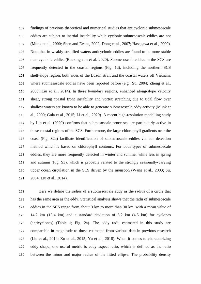
Here we define the radius of a submesoscale eddy as the radius of a circle that 122
has the same area as the eddy. Statistical analysis shows that the radii of submesoscale 123
eddies in the SCS range from about 3 km to more than 30 km, with a mean value of 124
14.2 km (13.4 km) and a standard deviation of 5.2 km (4.5 km) for cyclones 125
(anticyclones) (Table 1; Fig. 2a). The eddy radii estimated in this study are 126
comparable in magnitude to those estimated from various data in previous research 127
(Liu et al., 2014; Xu et al., 2015; Yu et al., 2018). When it comes to characterizing 128
eddy shape, one useful metric is eddy aspect ratio, which is defined as the ratio 129
between the minor and major radius of the fitted ellipse. The probability density 130

function of the aspect ratios of submesoscale eddies contains a skewed distribution 131
(Fig. 2b), with an average of 0.48 (0.49) and a standard deviation of 0.18 (0.18) for 132
cyclones (anticyclones) (Table 1). Interestingly, the eddy aspect ratio is found to be a 133
function of the eddy radius, irrespective of the eddy polarity (Fig. 2c); the larger the 134
submesoscale eddies, the more circular they are. 135
3.2. Horizontal Structure 136
The identified eddy edges are also used to investigate the horizontal structure of 137
submesoscale eddies. We first create a rotated coordinate system for the eddies, where 138
the coordinate center is defined as the center of each eddy, with the major (minor) 139
axis of the eddy on the x-axis (y-axis) (Supporting Information; Fig. S4). After that, 140
we project the edges of cyclonic and anticyclonic submesoscale eddies separately 141
onto the rotated eddy coordinate (Figs. 3a, b and S5). The average edges of cyclonic 142
and anticyclonic submesoscale eddies are found to be almost identical, revealing a 143
nearly perfect ‘cat’s-eye’ structure as shown in previous theoretical and numerical 144
studies (Munk et al., 2000; Shen and Evans, 2002). We then compare the observed 145
mean edges of submesoscale eddies with the Stuart solution 146
𝜓 = −𝑈/𝑘 ∙ 𝑙𝑜𝑔(cosh(𝑘𝑦) − 𝛼 ∙ cos(𝑘𝑥)), where U=±0.3 m s-1
is the background 147
shear flow, 𝑘 ≈0.0003 m-1
is the ratio between 2𝜋 and eddy length scale, and 𝛼 is 148
an unknown parameter between 0 and 1 that needs to be determined (following Munk 149
et al., 2000). The Stuart solution yields parallel shear flows when 𝛼 =0 and 150
concentrated point vortices as 𝛼 approaching 1. By adjusting 𝛼 to obtain a best fit 151
of the Stuart solution to the observed eddies, both cyclonic and anticyclonic, we find 152
𝛼=0.6 gives a good agreement. Our result therefore provides the first statistical 153
observational evidence in support of the ‘cat’s-eye’ horizontal structure proposed by 154
Munk et al. (2000) for submesoscale eddies. 155
Given that the submesoscale eddy aspect ratio depends on eddy radius (Fig. 2c), 156
the value of 𝛼 in the Stuart solution may also vary with the radius of submesoscale 157
eddies. To test this conjecture, we divide the identified eddies into five bins, at an 158

interval of 5 km from 5 km to 30 km, according to the eddy radius. Then, we average 159
all the fitted ellipse edges of submesoscale eddies in each bin to estimate the 160
best-fitting 𝛼 for each bin. The value of 𝛼 is indeed found to vary with the 161
submesoscale eddy radius, increasing from over 0.4 to around 0.7, with slightly 162
smaller values for cyclones (Fig. 3c). Moreover, binning of 𝛼 as a function of the 163
radius of cyclonic (anticyclonic) submesoscale eddies displays a nearly linear 164
relationship, with 𝛼 = 0.015𝑟 + 0.322 ( 𝛼 = 0.015𝑟 + 0.344 ) where 𝑟 is the 165
radius of submesoscale eddies. The relationship between the eddy radius and 𝛼 166
found in this study can be used to improve the Stuart solution to better describe the 167
surface structure of submesocale eddies which may have implications for 168
submesoscale eddy parameterizations. 169
3.3. Composite chlorophyll and SST 170
To examine the impact of submesoscale eddies on surface tracer distributions, 171
the log10-transformed chlorophyll and SST data of the 10-year study period are first 172
high-pass filtered using a Gaussian filter (Ni et al., 2020) and then are projected and 173
averaged onto the rotated submesoscale eddy coordinate (Supporting Information; Fig. 174
S4). Note that the flank of an eddy with positive chlorophyll anomalies is taken as the 175
positive y-axis. Fig. 4a (b) shows the resulting composite chlorophyll anomalies 176
inside and around cyclonic (anticyclonic) submesoscale eddies detected in the SCS. 177
On average, the magnitude of log10-transformed chlorophyll anomalies induced by 178
submesoscale eddies is on the order of ±0.1 mg m-3
, which is comparable to the 179
magnitude of seasonal variations of surface chlorophyll anomalies averaged over the 180
SCS (Fig. S2b) but several times larger than that associated with mesoscale eddies 181
(Chelton et al., 2011; Gaube at al., 2014; He at al., 2019). We also note that the 182
composite chlorophyll anomalies indicate a ‘cat’s-eye’ shape and display a distinct 183
dipole pattern which consists of two rotational anomalies of opposite sign. Similar 184
dipole structure has been seen in the composite maps of tracer anomalies (i.e., 185
chlorophyll and SST) induced by mesoscale eddies, which is known to result from 186

lateral eddy advection of background tracer gradients (Chelton et al., 2011; Hausmann 187
and Czaja, 2012; Gaube et al., 2015). In regions of significant background chlorophyll 188
gradient, the effect of horizontal eddy rotation is to advect high (low) chlorophyll 189
concentration to the side of low (high) chlorophyll concentration and thereby result in 190
positive (negative) chlorophyll anomalies. Indeed, the composite maps of Figs. 4a and 191
b indicate the existence of distinct chlorophyll fronts at 𝑦 ≈ 0. 192
The composite SST anomalies associated with the identified cyclonic and 193
anticyclonic submesoscale eddies are shown in Figs. 4c and d, respectively. One 194
outstanding feature is that positive (negative) SST anomalies on the flanks of 195
submesoscale eddies are collocated with negative (positive) chlorophyll anomalies, 196
consistent with the fact that near the coast the chlorophyll concentration is higher 197
while the SST is colder. Furthermore, the signatures of submesoscale eddies in the 198
composite SST anomaly images tend to be more obscure when compared to 199
chlorophyll. One possible explanation is that there exist various formation 200
mechanisms for submesoscale eddies. For the mechanism of frontal instability, the 201
pattern of chlorophyll anomalies is expected to be similar to that of SST anomalies 202
(Munk et al., 2000; Klein and Lapeyre, 2009). For the mechanism of shear instability, 203
however, a different picture occurs. For example, submesosocale eddies caused by 204
flow-island interaction may occur in a relatively homogeneous temperature field (Fig. 205
S1f; Yu et al., 2018), and as a result the imprint of submesoscale eddies in the SST 206
anomalies are less pronounced. Previous research indeed found greater chlorophyll 207
variance at submesoscales than SST (Mahadevan, 2016). This is why we choose 208
chlorophyll rather than SST to identify subemesoscale eddies in our method. The 209
difference between submesoscale eddy signatures in chlorophyll and SST maps also 210
reflects the degree of conservativeness in their behaviour, which may need to be 211
accounted for when parameterizing the effect of submesoscale eddies in the tracer 212
equations. 213

4. Conclusions 214
In this work we have developed an automatic submesoscale spiral eddy 215
identification method based on high-resolution chlorophyll data and then applied it to 216
the SCS which is a marginal sea rich in submesoscale eddies. The detected 217
submesoscale eddies in the SCS are found to have a radius of 13±5 km and an aspect 218
ratio of 0.5±0.2, with a notable predominance of cyclones. We have shown that the 219
surface structure of submesoscale eddies displays the classical ‘cat’s-eye’ pattern and 220
further determined the key unknown parameter in the Stuart solution that describes 221
the shape of the cat’s-eye pattern. Submesoscale eddies are found to induce dipole 222
surface chlorophyll and SST anomalies via horizontal advection of background 223
chlorophyll and SST gradients. 224
The widespread existence of submesoscale eddies is believed to be important in 225
tracer transport, energy cascade, re-stratification and biological processes in the upper 226
ocean (Ubelmann and Fu, 2011; McWilliams, 2010; Haine and Marshall, 1998; 227
Mahadevan, 2016). However, the present global ocean and climate models have too 228
coarse spatial resolutions to resolve submesoscale processes and as such would rely 229
on parameterizing the effect of submesoscale eddies for the foreseeable future (e.g., 230
Fox-Kemper et al., 2011). The submesoscale eddy structure and statistics found in this 231
study may provide observation-based guidance for future development of 232
submesoscale eddy parameterizations. For example, anisotropy in submesoscale eddy 233
length scales, i.e., shorter length scale in the cross-front direction than along-front 234
direction, implies anisotropic submesoscale eddy diffusivity if the parameterization 235
scheme employs a mixing length approach. 236
The high-resolution Surface Water and Ocean Topography (SWOT) satellite 237
altimeter is scheduled to launch in 2021 (Qiu et al., 2017), which aims at resolving sea 238
level variability at submesoscales. Combining the chlorophyll-based submesoscale 239
eddy detection method developed in this study with SWOT-derived submesoscale sea 240
level anomalies should have potential to further improve our understanding of the 241

surface pattern, dynamics and impact of submesoscale eddies. Nevertheless, in 242
addition to satellite remote sensing, we still need in-situ observing technologies with 243
high-enough spatiotemporal resolution to reveal the three-dimensional structure of 244
these eddies. 245
Acknowledgments 246
X.Z. acknowledges support by a Royal Society International Exchanges Award 247
(IEC/NSFC/170007). C.W. is supported by the Climate Linked Atlantic Sector 248
Science (CLASS) project, which is itself supported by NERC National Capability 249
funding (NE/R015953/1). C.C. acknowledges support by the National Natural Science 250
Foundation of China (42076018). D.C. is supported by the National Natural Science 251
Foundation of China (41730535). Q.N. thanks Guihua Wang, Xuemin Jiang, Pengfei 252
Tuo, Sheng Lin and Zhibin Yang for their helpful discussions. The chlorophyll and 253
SST data are available at https://oceandata.sci.gsfc.nasa.gov/. 254
References 255
1. Buckingham, C. E., Gula, J., & Carton, X. (2020). The role of curvature in 256
modifying frontal instabilities, part 2. Journal of Physical Oceanography, 1-67. 257
2. Buckingham, C. E., Khaleel, Z., Lazar, A., Martin, A. P., Allen, J. T., Garabato, A. 258
C., Thompson, A. F., & Vic, C. (2017). Testing Munk's hypothesis for 259
submesoscale eddy generation using observations in the North Atlantic. Journal 260
of Geophysical Research, 122(8), 6725-6745. 261
3. Chelton, D. B., Schlax, M. G., & Samelson, R. M. (2011). Global observations of 262
nonlinear mesoscale eddies. Progress in Oceanography, 91(2), 167-216. 263
4. Dong, C., Mcwilliams, J. C., & Shchepetkin, A. F. (2007). Island Wakes in Deep 264
Water. Journal of Physical Oceanography, 37(4), 962-981. 265

5. Fox-Kemper, B., Danabasoglu, G., Ferrari, R., Griffies, S. M., Hallberg, R. W., 266
Holland, M. M., Maltrud, M. E., Peacock, S., & Samuels, B. L. (2011). 267
Parameterization of mixed layer eddies. III: Implementation and impact in global 268
ocean climate simulations. Ocean Modelling, 39, 61-78. 269
6. Gaube, P., Chelton, D. B., Samelson, R. M., Schlax, M. G., & O’Neill, L. W. 270
(2015). Satellite observations of mesoscale eddy-induced Ekman pumping. 271
Journal of Physical Oceanography, 45(1), 104-132. 272
7. Gaube, P., Mcgillicuddy, D. J., Chelton, D. B., Behrenfeld, M. J., & Strutton, P. G. 273
(2014). Regional variations in the influence of mesoscale eddies on near-surface 274
chlorophyll. Journal of Geophysical Research, 119(12), 8195-8220. 275
8. Gula, J., Molemaker, M. J., & Mcwilliams, J. C. (2015). Topographic vorticity 276
generation, submesoscale instability and vortex street formation in the Gulf 277
Stream. Geophysical Research Letters, 42(10), 4054-4062. 278
9. Haine, T. W. N., & Marshall, J. (1998). Gravitational, symmetric, and baroclinic 279
instability of the ocean mixed layer. Journal of Physical Oceanography, 28(4), 280
634-658. 281
10. Hasegawa, D., Lewis, M. R., & Gangopadhyay, A. (2009). How islands cause 282
phytoplankton to bloom in their wakes. Geophysical Research Letters, 36(20), 283
L20605. 284
11. Hausmann, U., & Czaja, A. (2012). The observed signature of mesoscale eddies 285
in sea surface temperature and the associated heat transport. Deep Sea Research 286
Part I, 70, 60-72. 287
12. He, Q., Zhan, H., Xu, J., Cai, S., Zhan, W., Zhou, L., & Zha, G. (2019). 288
Eddy-induced chlorophyll anomalies in the western South China Sea. Journal of 289
Geophysical Research, 124, 1-20. 290

13. Hu, J., & Wang, X. H. (2016). Progress on upwelling studies in the China seas. 291
Reviews of Geophysics, 54(3), 653-673. 292
14. Thomson, W. (1880) On a disturbing infinity in Lord Rayleigh’ s solution for 293
waves in a plane vortex stratum. Nature, 23, 45-46. 294
15. Klein, P., & Lapeyre, G. (2009). The oceanic vertical pump induced by mesoscale 295
and submesoscale turbulence. Annual Review of Marine Science, 1(1), 351-375. 296
16. Li, G., He, Y., Liu, G., Zhang, Y., Hu, C., & Perrie, W. (2020). Multi-sensor 297
observations of submesoscale eddies in coastal regions. Remote Sensing, 12(4): 298
711. 299
17. Lin, H., Liu, Z., Hu, J., Menemenlis, D., & Huang, Y. (2020). Characterizing 300
meso- to submesoscale features in the South China Sea. Progress in 301
Oceanography, 118, 102420. 302
18. Liu, F., Tang, S., & Chen, C. (2014). Satellite observations of the small-scale 303
cyclonic eddies in the western South China Sea. Biogeosciences, 12(2), 299-305. 304
19. Mahadevan, A. (2016). The Impact of Submesoscale Physics on Primary 305
Productivity of Plankton. Annual Review of Marine Science, 8(1), 161-184. 306
20. McWilliams, J. C. (2010). A perspective on submesoscale geophysical turbulence. 307
IUTAM Symposium on Turbulence in the Atmosphere and Oceans, 131-141. 308
21. Munk, W., Armi, L., Fischer, K. W., & Zachariasen, F. (2000). Spirals on the sea. 309
Proceedings of The Royal Society A: Mathematical, Physical and Engineering 310
Sciences, 456(1997), 1217-1280. 311
22. Ni, Q., Zhai, X., Wang, G., & Marshall, D. P. (2020). Random movement of 312
mesoscale eddies in the global ocean. Journal of Physical Oceanography, 50(8), 313
2341-2357. 314

23. Oram, J. J., Mcwilliams, J. C., & Stolzenbach, K. D. (2008). Gradient-based edge 315
detection and feature classification of sea-surface images of the Southern 316
California Bight. Remote Sensing of Environment, 112(5), 2397-2415. 317
24. Qiu, B., Nakano, T., Chen, S., & Klein, P. (2017). Submesoscale transition from 318
geostrophic flows to internal waves in the northwestern Pacific upper ocean. 319
Nature Communications, 8, 14055. 320
25. Shen, C. Y., & Evans, T. E. (2002). Inertial instability and sea spirals. 321
Geophysical Research Letters, 29(23), 39-1-39-4. 322
26. Stuart, J. T. (1967). On finite amplitude oscillations in laminar mixing layers. 323
Journal of Fluid Mechanics, 29, 417-440. 324
27. Su, J. (2004). Overview of the South China Sea circulation and its influence on 325
the coastal physical oceanography outside the Pearl River estuary. Continental 326
Shelf Research, 24(16), 1745-1760. 327
28. Ubelmann, C., & Fu, L. (2011). Cyclonic eddies formed at the Pacific tropical 328
instability wave fronts. Journal of Geophysical Research, 116, C12021. 329
29. Wang, G., Su, J., & Chu, P. C. (2003). Mesoscale eddies in the South China Sea 330
observed with altimeter data. Geophysical Research Letters, 30(21), 2121. 331
30. Xu, G., Yang, J., Dong, C., Chen, D., & Wang, J. (2015). Statistical study of 332
submesoscale eddies identified from synthetic aperture radar images in the Luzon 333
Strait and adjacent seas. Journal of remote sensing, 36(18), 4621-4631. 334
31. Yu, J., Zheng, Q., Jing, Z., Qi, Y., Zhang, S., & Xie, L. (2018). Satellite 335
observations of sub-mesoscale vortex trains in the western boundary of the South 336
China Sea. Journal of Marine Systems, 183, 56-62. 337
32. Zheng, Q., Lin, H., Meng, J., Hu, X., Song, Y. T., Zhang, Y., & Li, C. (2008). 338

Sub-mesoscale ocean vortex trains in the Luzon Strait. Journal of Geophysical 339
Research, 113, C04032. 340
341

Table 342
Table 1. Statistical features of submesoscale eddies detected in the South China Sea 343
from 2006 to 2015 344
Polarity r (km) 𝑟𝑚𝑖𝑛/𝑟𝑚𝑎𝑗
Mean STD Mean STD
Cyclonic 14.2 5.2 0.48 0.18
Anticyclonic 13.4 4.5 0.49 0.18
345

Figures 346
347
Figure 1. (a) Particle distribution (black dots and colour curves) in a Stuart spiral eddy 348
(black dashed contour) that shows a ‘cat’s-eye’ pattern. Adapted from Munk et al. 349
(2000). (b) One-day snapshot of cyclonic submesoscale eddies (blue curves) 350
identified from high-resolution chlorophyll data (colour shading; mg m-3
). The eddy 351
edges are denoted by black dashed curves. (c) Same as Fig. 1b but for an anticyclonic 352
submesoscale eddy (red curves). (d) Distributions of cyclonic (blue dots) and 353
anticyclonic (red dots) submesoscale eddies identified in the South China Sea (SCS) 354
from 2006 to 2015. 355
356

357
Figure 2. (a) Histogram of the radius of submesoscale eddies in the SCS. (b) Same as 358
Fig. 2a but for the eddy aspect ratio that is defined as the ratio between the minor and 359
major radius of a submesoscale eddy. (c) Variations of eddy aspect ratio with eddy 360
radius (averaged in an eddy-radius bin of 5 km). Vertical lines denote one standard 361
deviation. 362
363

364
Figure 3. Horizontal structure of submesoscale eddies in the SCS. (a) Edges of 365
cyclonic eddies (blue curves) and their average (white curve) on a rotated 366
submesoscale eddy coordinate system (Supporting Information). Black dashed 367
contours are the horizontally normalized streamfunction contours derived from the 368
Stuart solution 𝜓 = −𝑈/𝑘 ∙ 𝑙𝑜𝑔(cosh(𝑘𝑦) − 𝛼 ∙ cos(𝑘𝑥)), where 𝑈=±0.3 m s-1
, 369
𝑘 ≈0.0003 m-1
, and 𝛼=0.6. (b) Same as Fig. 3a but for anticyclonic eddies (red 370
curves). (c) Values of 𝛼 as a function of the radius of cyclonic (blue dots) and 371
anticyclonic (red dots) submesoscale eddies and the corresponding linear fitting 372
results (lines). 373
374

375
Figure 4. (a, b) Composite log10-transformed chlorophyll anomalies (mg m-3
) on the 376
rotated submesoscale eddy coordinate. (c, d) Same as Fig. 4a, b but for SST anomalies 377
(°C). 378