Embed Size (px)
Citation preview

1
MSc in Computing, Business Intelligence and Data Mining stream.
Business Intelligence and Data Mining Applications Project Report.
Predicting earning potential on Adult Dataset
Submitted by: xxxxxxx
Supervisor: Markus Hofmann
Submission date 21/05/2011

2
Declaration I herby certify that this material, which I now submit for assessment on the
programme of study leading to the award of MSc in Computing in the Institute of
Technology Blanchardstown, is entirely my own work except where otherwise
stated, and has not been submitted for assessment for an academic purpose at
this or any other academic institution other than in partial fulfillment of the requirements of that stated above.
Author: __xxxxxxxx______ Dated: __21/5/2011___

3
Abstract This report implements the CRISP-DM methodology when applying classification models to the problem of identifying individuals whose salary exceeds a specified value based on demographic information such as age, level of education and current employment type. The process involved in the exploration, preparation, modelling and evaluation of the datasets are described. Topics such as the application of statistical analysis to suggest attribute usefulness, feature reduction, outlier detection, missing value management, data bias and data transformation are discussed. The process of relative performance analysis of the proposed classifiers is reviewed. The support of a business objective which will use the predictive capabilities of the proposed models to target customers is reviewed including the use of lift analysis to indicate the likely level of return on investment and overall profitability.

4
Table of Contents
Page Introduction 6 Business Understanding 6 Business objective 6 Data Mining objective 7 Project plan 7 Data Understanding 7 Describe the data 7 Explore the data 8 Verify data quality 14 Data Preparation 15 Select Data 15 Construct Data 16 Modelling 19 Select modelling technique 19 Generate Test Design 19 Build and Assess the model 19 Evaluation 28 Appendix A 30 References 30 List of Tables 1 Description of dataset 9 2 Numerical attribute quantiles, unique values and outliers 11 3 Mapping between education number and education level attributes 11 4 Comparison of occupation attribute values within the salary classes 13 5 Rules discovered for >50K salary class on training dataset 14 6 Naïve Bayes with forward selection, SVD and PCA 16 7 Relationship and marital status attribute transformations 17 8 Entropy binning output 17 9 Numerical attribute binning 18 10 Naïve Bayes performance (iteration 2) 20 11 Naïve Bayes and hybrid classifier performance 20 12 Discretisation applied to NBTree classifier 22 13 kNN k values 22

5
14 kNN performance 22 15 Mean values cost attribute clusters 25 16 Classifier evaluation on test dataset 25 17 Classifier Lift results 26 List of Diagrams 1 Boxplots of numeric attributes 10 2 Regression classifier output 11 3 Training dataset correlation matrix 12 4 Histogram of education levels 12 5 Histograms of age for gender and salary 12 6 Decision tree output 13 7 Outlier deviation plot 14 8 Initial ROC curves 15 9 Data transformations type A 18 10 Data transformations type B 19 11 Hybrid classifier ROC curves 20 12 NBTree classifier output 21 13 Data transformations type C 23 14 Hybrid ROC curves on transformed data 23 15 MetaCost scatter plot 24 16 Return on investment plots 27 17 Profitability plots 27

6
1. Introduction This project will investigate the data mining of demographic data in order to create one or more classification models which are capable of accurately identifying individuals whose salary exceeds a specified value. The data used in this project were sourced from the University of California Irvine data repository and are referred to as the Adult dataset and contain information on individuals such as age, level of education and current employment type. The classification model will be used to select candidates for a new service offered by the sponsor of the project targeting individuals with salaries exceeding fifty thousand US dollars. A description of the predictive significance of each attribute, interesting or useful patterns which were found and any transformations applied to the data must be provided with all proposed models. This report will describe the work carried out during the iterative process of data preparation, modelling and evaluation including data formatting, consistency or other quality issues, opportunities for useless instance or attribute removal and the approaches taken to solving issues with instances affected by noise, outliers or missing values.
This project will implement the CRISP-DM methodology where a comprehensive review of the customer's requirements supports the creation of a business objective outlining items such as the expected level of model performance and return on investment. This will be used to create a data mining objective which will guide the subsequent work in the data understanding, preparation and modelling steps and the final evaluation and selection (after revisiting earlier steps if necessary) of a classification model or models. 2. Business Understanding Business objective A project team has been created to support the marketing of a new service targeted at potential customers with medium to high level salaries. There is an initial project setup cost of eighteen thousand dollars, a cost of one hundred and twenty five dollars for each offer made and a return of five hundred dollars for each accepted offer: Setup cost: $18,000 Cost per offer: $125 Return per accepted offer: $500 The current marketing strategy, which involves a high degree of investment per offer (driving the relatively high offer cost) has achieved a high acceptance rate in the past of seventy five percent by individuals whose salaries exceed fifty thousand US dollars. The goal of this project is therefore to create a model (or models) which can accurately identify individuals whose annual salary exceeds this amount. Any proposed model must

7
be capable of significantly outperforming the existing candidate selection model which is currently providing an average return on investment of seventy to ninety. Data Mining objective The data mining objective is to create a classification model which can predict individuals whose salary exceeds fifty thousand US dollars by mining anonymised census data containing demographic information such as age, gender, education level and employment type. The original salary attribute in the census data has been anonymised to a binomial value indicating if a salary exceeds fifty thousand US dollars. For each proposed model an expected return on investment (and associated profit margins) must be provided. A clear description of all data transformations which were carried out must be provided and any useful insights into the data such as significant attributes or mining issues within the data should be included. Project plan Phase Date Details Status A 20/2/2011 Start date Closed B 28/2/2011 Project proposal compete Closed C 5/3/2011 Crisp 1: Business understanding Closed D 12/3/2011 Crisp 2: Initial data understanding Closed E 20/3/2011 Crisp 3: Initial data preparation (and testing Closed with early modelling) F 30/03/2011 Interim presentation based on phases A to D Closed Crisp 4: Creation/test of models (update results Closed in D and E as required) G 06/04/2011 Crisp 4: Ongoing testing of data preparation (update Closed results in D to F as required) H 20/04/2011 Crisp 5: Evaluation of proposed models Closed I 1/5/2011 Final presentation of work Closed Create project report Closed J 16/5/2011 Completion date 3. Data Understanding Describe the data The dataset used in this project has forty nine thousand records and a binomial label indicating a salary of less or greater than fifty thousand US dollars, which for brevity, will be referred to as <50K or >50K in this report. Seventy six percent of the records in the dataset have a class label of <50K. The data has been divided into a training dataset containing thirty two thousand records and a test dataset containing sixteen thousand records.

8
There are fourteen attributes consisting of seven polynomials, one binomial and six continuous attributes (Table 1). The nominal employment class attribute describes the type of employer such as self employed or federal and occupation describes the employment type such as farming or managerial. The education attribute contains the highest level of education attained such as high school graduate or doctorate. The relationship attribute has categories such as unmarried or husband and the marital status attribute has categories such as married or separated. The final nominal attributes are country of residence, gender and race. The continuous attributes are age, hours worked per week, education number (which is a numerical representation of the nominal education attribute), capital gain and loss and a survey weight attribute which is a demographic score assigned to an individual based on information such as area of residence and type of employment. Explore the data The standard deviations in the data (Table 1) indicates that there is a significant quantity of values in all attributes, particularly in the case of the survey weight attribute and the high kurtosis in the capital gain attribute indicates a long tail. From the boxplots it can be seen that the range of attribute values for age, education number and hrs_per_week (worked) is slightly higher in >50K class instances (Figure 1) indicating that these attributes may have predictive significance.

9
Table 1. Description of dataset.

10
Figure 1. Boxplots of numeric attributes The numeric attributes appear to contain a significant quantity of unique values (Table 2) and in the case of the survey weight attribute there were twenty one thousand unique values out of thirty one thousand instances, which may suggest that this attribute may not be significantly predictive. This was confirmed when a regression model was applied to the dataset where fnlwgt had a t-Statistic of zero and a p-Value of one (Figure 2). The other attributes were found to be reasonably significant with the exception of the country attribute (which contains a value of 'United-States' in ninety percent of instances) and the race attribute (which contains a value of 'White' in eighty five percent of instances), and may be candidates for removal during data preparation, and the marital status attribute which is explored further later in this report.

11
Figure 2. Regression classifier output on training dataset. Table 2. Numerical attribute quantiles, unique values and outliers
Although the capital gain and loss attributes have significant quantities of unique values (Table 2), the majority of the instances have a zero value with capital gain having ninety six percent zero values in the <50K class and seventy nine percent in the >50K class and capital loss having ninety eight percent in the <50K class and ninety percent in the >50K class. This may indicate that these attributes also may not be very predictive. The numeric education number and nominal education level attributes were found to be fully correlated and therefore one of these attributes may be a good candidate for removal during modelling (Table 3). In general the other attributes were found to be weakly correlated (Figure 3). When the education number attribute was plotted for the class labels it was found that the lower values tend to predominate in the <50K class and higher levels in the >50K class which may indicate some predictive capability (Figure 4). Table 3. Mapping between education number and education level attributes

12
Figure 3. Correlation matrix for the training dataset.
Figure 4. Normalised histogram of education level in class labels. A slight bias was detected in the dataset where instances with a 'female' gender value have lower range of age values than instances with a 'male' gender value (Figure 5A). This may skew the predictive capability of the gender attribute to some degree as age values within >50K class instances tend to be higher (Figure 5B) than <50K instances. There is also a slight imbalance in gender with sixty seven percent of instances having a male value (Table 1).
Figure 5. Histograms of age profile for gender and salary attributes
13
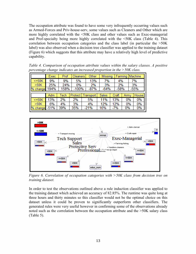
The occupation attribute was found to have some very infrequently occurring values such as Armed-Forces and Priv-house-serv, some values such as Cleaners and Other which are more highly correlated with the <50K class and other values such as Exec-managerial and Prof-specialty being more highly correlated with the <50K class (Table 4). This correlation between occupation categories and the class label (in particular the >50K label) was also observed when a decision tree classifier was applied to the training dataset (Figure 6) which suggests that this attribute may have a relatively high level of predictive capability. Table 4. Comparison of occupation attribute values within the salary classes. A positive percentage change indicates an increased proportion in the >50K class.
Figure 6. Correlation of occupation categories with >50K class from decision tree on training dataset. In order to test the observations outlined above a rule induction classifier was applied to the training dataset which achieved an accuracy of 82.85%. The runtime was quite long at three hours and thirty minutes so this classifier would not be the optimal choice on this dataset unless it could be proven to significantly outperform other classifiers. The generated rules were very useful however in confirming some of the observations already noted such as the correlation between the occupation attribute and the >50K salary class (Table 5).

14
Table 5. Rules discovered for >50K salary class on training dataset.
Verify data quality In general it was found that the incidence of extreme outliers in the dataset was low with the exception of the hours_per_week (worked) attribute which has a significant percentage of outliers in both tails. The age and fnlwgt (survey weight) attributes had outliers in less than three percent of instances (Table 2). Rapidminer's Detect Outlier (Distances) operator (with a k value of six based on kNN classifier modelling) detected outliers primarily in the fnlwgt (survey weight) and capital gain attributes (Figure 7).
Figure 7. Deviation plot of the mean and range of values in outlier (true) and non-outlier (false) instances based on a mixed euclidean measures.
15
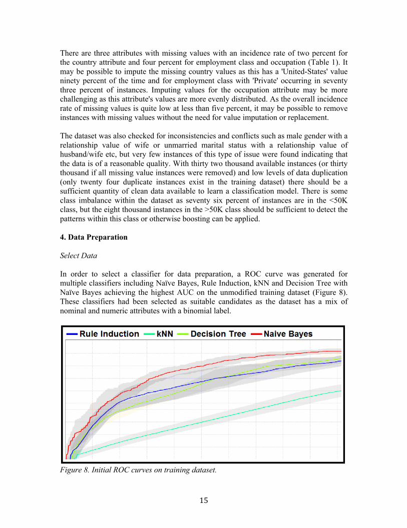
There are three attributes with missing values with an incidence rate of two percent for the country attribute and four percent for employment class and occupation (Table 1). It may be possible to impute the missing country values as this has a 'United-States' value ninety percent of the time and for employment class with 'Private' occurring in seventy three percent of instances. Imputing values for the occupation attribute may be more challenging as this attribute's values are more evenly distributed. As the overall incidence rate of missing values is quite low at less than five percent, it may be possible to remove instances with missing values without the need for value imputation or replacement. The dataset was also checked for inconsistencies and conflicts such as male gender with a relationship value of wife or unmarried marital status with a relationship value of husband/wife etc, but very few instances of this type of issue were found indicating that the data is of a reasonable quality. With thirty two thousand available instances (or thirty thousand if all missing value instances were removed) and low levels of data duplication (only twenty four duplicate instances exist in the training dataset) there should be a sufficient quantity of clean data available to learn a classification model. There is some class imbalance within the dataset as seventy six percent of instances are in the <50K class, but the eight thousand instances in the >50K class should be sufficient to detect the patterns within this class or otherwise boosting can be applied. 4. Data Preparation Select Data In order to select a classifier for data preparation, a ROC curve was generated for multiple classifiers including Naïve Bayes, Rule Induction, kNN and Decision Tree with Naïve Bayes achieving the highest AUC on the unmodified training dataset (Figure 8). These classifiers had been selected as suitable candidates as the dataset has a mix of nominal and numeric attributes with a binomial label.
Figure 8. Initial ROC curves on training dataset.

16
To investigate the applicability of feature reduction to the full training dataset forward selection was applied to a Naïve Bayes classifier (Table 6 A). The results of this test indicate that although the >50K class precision was improved slightly over Naïve Bayes (without forward selection) the overall performance was degraded slightly (Table 6 B). The application of forward selection did however provide useful information as the fnlwgt (survey weight) and country attributes had been dropped without significantly impacting the performance of the Naïve Bayes classifier confirming the earlier assertion during data exploration that these attributes may not be significantly predictive. Singular value decomposition (SVD) and principle component analysis (PCA) were then applied to the dataset in two ways. Initially SVD and PCA (with an optimal quantity of three dimensions/ components) were applied to the numerical attributes only which were joined to the nominal attributes and passed to a Naïve Bayes classifier with both achieving an eighty two percent accuracy (Table 6 C/E). SVD and PCA (with an optimal quantity of six dimensions/components) were then applied to all attributes, where the nominal attributes had been mapped to real values, and both approaches now achieved an accuracy of seventy nine percent (Table 6 D/F). These results indicate that the above approaches to feature reduction on the unmodified training dataset do not appear to be useful in improving classifier accuracy. Table 6. Naïve Bayes with forward selection, SVD and PCA on training dataset.
Construct Data When the marital status and relationship attribute values were modified slightly to reduce the number of categories (Table 7) it was observed that the information in the marital status attribute could be inferred to some degree from the 'unmarried' category in the relationship attribute suggesting that marital status might be a candidate for removal. Discretisation was applied to the numerical attributes to determine if the performance of the Naïve Bayes classifier could be improved. Initially entropy binning was investigated on the training dataset but a performance of eighty two percent was poorer than that achieved without binning. However the output (Table 8) from this exercise did provide a useful starting point in suggesting bin boundaries for the following discretisation work.

17
Table 7. Relationship and marital status attribute transformations.
Table 8. Entropy binning output on training dataset.
By iteratively testing various bin boundary combinations using Rapidminer's Optimise Parameter operator an optimal bin quantity for the hrs_per_week (worked) attribute was found to be twenty with the most highly populated bin (by a factor of ten) having bin boundaries of thirty five and forty with a mean of thirty nine. It was found that using a two bin approach with a bin boundary of this mean value of thirty nine proved to be equally effective. (Table 9). Using the binning operator in rapidminer the optimal bin quantity for the age attribute was found to be eleven (Table 9) and based on the generated bin boundaries and work with R to determine the data distribution twenty bins were selected at boundaries ranging from twenty to sixty six (specifically 20, 25, 31, 36, 40, 46, 51, 56, 60, 66 and over 66) which slightly improved the classifier's performance. The more variate capital gain and loss attributes were found to have optimal binning quantities of five hundred and fifteen hundred respectively as increasing the bin quantity beyond this points did not improve the model's performance significantly (Table 9).

18
Table 9. Numerical attribute binning results
During initial modelling on the training dataset with Naïve Bayes it was found that removing the country (which has the same value in ninety percent of cases), education number (which is correlated with education level), survey weight (which is highly variate) and marital status (which appears to contain similar information to the relationship attribute as outlined earlier) attributes did not affect the model's performance. Therefore these four attributes will be considered for removal during future modelling. The results of these initial data transformations are summarised below and will be referred to in this report as data transformations type A (Figure 9).
Figure 9. Data transformations type A

19
5. Modelling Select modelling technique As stated above as the dataset has mixed numerical and nominal attributes with a binomial class label a Decision Tree, kNN, Naïve Bayes and Rule Induction classifier had been selected for initial modelling. Generate Test Design During modelling the training dataset will initially be used to evaluate each classifier's performance relative to that achieved by Naïve Bayes on the unmodified training dataset (Table 6 A) and the optimal classifiers will then be evaluated on the test dataset in terms of overall performance and ability to support the primary business objective of maximising the return on investment. Build and Assess the model As described in the data preparation section above applying forward selection on the unmodified training dataset with Naïve Bayes had not been very successful (Table 6) it was decided during modelling to revisit this idea but this time the data transformations (Type A) above were applied ahead of forward selection. This approach proved to be quite successful with a Naïve Bayes performance improvement of three percent (Table 10). Examination of the model's example-set showed that forward selection on the transformed data had also additionally removed the hrs_per_week, age, occupation and gender attributes which will be referred to as data transformations type B in this report (Figure 10).
Figure 10. Data transformations type B

20
Table 10. Naïve Bayes performance on the training dataset with unmodified data, data with forward selection only and with forward selection to the transformed data.
As additional attribute transformations did not further improve the performance of the Naïve Bayes classifier the WEKA extension was imported into Rapidminer in order to access some hybrid tree classifiers. As Naïve Bayes had performed well on the training dataset the NBTree and DTNB classifiers appeared to be good candidates as they both combine Naïve Bayes with a decision tree which may provide useful insights into the data even if further performance improvements are not achieved. DTNB is a cost-sensitive learner which attempts to minimize mis-classification costs using a single Naïve Bayes classifier in the background to assist in making globally influenced branching decisions at the nodes. The NBTree classifier is slightly different in that it creates a Naïve Bayes classifier at each node in order to determine how the node should be split. The DTNB and NBTree did indeed prove to be the best performing classifiers in the Rapidminer WEKA classifier set on the unmodified training dataset and out-performed Naïve Bayes (Table 11 and Figure 11). Table 11. Naïve Bayes and hybrid classifier performances on unmodified training dataset
Figure 11. ROC curves on unmodified training dataset.

21
The rules generated in the NBTree output (Figure 12) were quite useful in determining attribute significance which was broadly in agreement with what had been discovered using other classifiers.
Figure 12. NBTree classifier output on training dataset. The portion of the tree shown reflects the rules indicated in the highlighted area where each leaf contains a local implementation of a Naïve Bayes classifier. The data transformations outlined above were then applied to the NBTree classifier on training dataset with the type A data transformations achieving 86.73% (Table 12 F) and the type B transformations achieving a slightly lower accuracy of 86.07% (Table 12 G). For comparison purposes forward selection with no data transformations was then applied to NBTree which had an accuracy of 86.14% (Table 12 H) which falls within the range of accuracies achieved with data transformation type A. Finally the type A transformations were applied to the DTNB classifier which achieved a similar accuracy to NBTree of 86.68% (Table 12 I).

22
Table 12. Discretisation applied to NBTree classifier on training dataset.
Although kNN had performed quite poorly on the unmodified dataset (Figure 8) it was decided (as per the CRISP-DM framework) to return to the data preparation stage and apply the data transformations outlined above to kNN. The first step was the selection of an optimal value for k which was found to be six based on the classifier's accuracy on a sample of the training dataset (Table 13). Table 13. kNN performance for k values from 3 to 7 on unmodified training dataset.
It was found that the type A transformations required some modification to achieve an optimal performance with kNN, where the discretisation on capital gain and loss was removed (as kNN preferred this lower level of data granularity) and missing values were removed, which were not an issue for Naïve Bayes. This improved kNN's performance from 79% to 85% (Table 14) and provided further independent validation of the usefulness of the proposed data transformations. The data transformations applied to kNN will be referred to as data transformations type C (Figure 13). Table 14. kNN (k=6) classifier performance.

23
Figure 13. Data transformations type C The ROC curve also indicated a much improved performance with kNN with the type C transformation as it now lies between the NBTree and Naïve Bayes ROC curves (Figure 14). The original ROC curve for kNN on the unmodified training dataset (kNN(Original) has also been included in the ROC curves for comparison purposes with an AUC little better than 0.5.
Figure 14 ROC curves of NBTree, Naïve Bayes and kNN (for both transformed and unmodified training data).

24
In order to evaluate the performance of a cost sensitive classifier a MetaCost operator was then applied to the training dataset. The cost matrix contained a value of one hundred and twenty five in the lower left which is the cost per offer and a value of minus five hundred in the lower right which is the potential maximum revenue per correct classification. It was found that an optimal performance was achieved when MetaCost was used with a logistic model tree (LMT). An LMT classifier replaces sub-trees with linear regression functions if the data subset at that node is suitable for this type of classification. A goal of LMT is to avoid overfitting as we work down into smaller subsets of data within the tree and to simplify the overall structure of the tree without impacting performance. This model worked quite well on the training dataset with a performance of 80% and applying the data transformations outlined above did not significantly improve performance. This classifier had a runtime of over four hours on the training dataset which means that a significant performance gain on other classifiers would be required to justify it's selection which was not the case here. This classifier was also applied to the test dataset as described later in this report. One interesting observation with the MetaCost(LMT) classifier was that the cost attribute in the output appeared to form two clusters (Figure 15) where the lower cluster would contain instances with a higher probability of being in the >50K salary class.
Figure 15. Scatter plot of MetaCost output cost attribute for >50K label instances

25
To explore this further the cluster attribute means were calculated for instances with cost values greater than minus two hundred and for instances with cost values less (more negative) than minus four hundred and fifty (Table 15). The differences in the attribute means indicated that the capital gain and loss attributes were significantly correlated (as demonstrated by the mean deltas) with the >50K class label. Further work in this area could involve mapping the nominal attributes to meaningful real values to determine the degree of mean differences between the class labels but that work is beyond the scope of this report. Table 15. Mean values of >50K salary class cost attribute clusters.
The four best performing classifiers found during the modelling phase (Naïve Bayes, NBTree, MetaCost(LMT) and kNN) were then evaluated on the test dataset with the appropriate data transformations as outlined above. It was found that NBTree had the best overall performance (Table 16). Naïve Bayes had the lowest runtime at one minute, followed by NBTree at three minutes, kNN at fifteen minutes and the MetaCost(LMT) at three hours. Table 16. Classifier performance on test dataset.
The lift for each classifier was then calculated on the test dataset in order to evaluate relative performances with respect to the business objective of maximising return on investment and overall profitability (Table 17).

26
Table 17. Classifier lift numbers on the test dataset. 'Bin Qty' is the total number of prospects in each of the ten bins and the 'Salary>50K' quantity is the expected number of correctly classified >50K instances.
Based on this lift data the overall return on investment (Figure 16) and profitability (Figure 17) were calculated per bin for each model (Appendix A contains a worked example of these calculations). The kNN classifier (with type C data transformations) consistently returned the highest return on investment with a maximum value of at one hundred and fifty nine when offers were sent to prospects in the first lift bin only. The NBTree model (with type A data transformations) was the most profitable in real terms with offers sent to prospects in the first three bins generating an expected revenue of one million one hundred thousand dollars for an initial investment of six hundred and twenty thousand dollars. These calculations are based on the relatively small test dataset which was used in this project and would be expected to scale up when applied to larger datasets. For comparison purposes the profitability and return on investment was calculated for each bin in a 'No Model' scenario based on the assumption that each bin contains twenty four percent >50K instances (which reflects the degree of occurrence in the general population) which had a negative return on investment and was a loss making exercise regardless of the number of prospects contacted.

27
Figure 16. Classifier return on investment per bin on test dataset.
Figure 17. Classifier profitability per bin on test dataset.

28
6. Evaluation During the CRISP-DM data understanding phase of the project some of the attributes were found to be predominantly single valued such as the country (with 'United-States') and capital gain and loss (with 0) in over ninety percent of instances. The survey weight attribute had the opposite issue where there was a large number of unique values. Later work with forward selection on Naïve Bayes confirmed that the country and survey weight attributes could be removed successfully without impacting classifier performance. The numeric education number and nominal education level attributes were found to be fully correlated (with education number being removed later during data preparation), and a correlation was also discovered between the marital status and relationship attributes after some basic category aggregation had been carried out and also between categories in the occupation attribute and the >50K class label. The overall data quality was quite good with a low occurrence of conflicting attribute values and with over thirty thousand clean instances in the training dataset and fifteen thousand in the training dataset (with both having low levels of data duplication) there was a sufficient quantity of clean variate data in both class labels to successfully create (with training data) and evaluate (with test data) the various classifiers. Some outliers were detected in the data but this was not found to seriously impact classifier performance as the percentage of affected instances was low in general with the hours_per_week (worked) attribute having slightly elevated levels but as binning was found to be beneficial on this attribute the impact of outliers was reduced. The percentage of records with missing values was quite low with country at two percent and employment class and occupation at four percent which did not affect the classification work except in the case of kNN where the affected instances were successfully removed. Some biases were detected in the data such as female (gender attribute) instances generally having a lower set of values than male instances but incidences of this type were not found to be significant. The general observations made during data exploration were confirmed when an initial rule induction classifier was applied to the training data and again when the NBTree output was analysed. When the models which were deemed to be appropriate for this dataset (with mixed numerical and nominal attributes and a binomial label) were applied to the unmodified training data the Naïve Bayes classifier had the best performance. During initial data preparation it was found that the optimal data transformation for Naïve Bayes involved discretising the hrs_per_week (worked), age, capital gain and capital loss attributes and removing the country, education number, survey weight and marital status attributes (which had been noted as possible candidates for removal earlier). This useful data transformation was tagged as type A in this report. When the type A data transformation was applied ahead of forward selection on a Naïve Bayes classifier a further performance improvement was achieved by additionally removing the hrs_per_week, age, occupation and gender attributes which was tagged as type B data transformation.

29
The type A data transformations were then applied to the hybrid DTNB and NBTree classifiers on the training dataset with improved performance on both and a slight modification to the type A (where the discretisation on the capital gain and loss attributes was removed as were instances with missing values) proved optimal for the kNN classifier which was tagged as type C data transforms. The modelling work on the training dataset appears to indicate that there is a classifier accuracy limit of just below eighty seven percent which is supported by other work such as the Naïve Bayes performance given at eighty three to four percent with discretisation (Kaya, 2008) and also at eighty four percent (Kohavi, 1996) and NBTree results posted by UCI (UCI Archive, 2011) indicating a performance of eighty five percent. It therefore appears that the proposed models and associated data transforms outlined in this report are close to optimal. During the modelling phase the training dataset had been used to evaluate the relative performance of each of the selected classifiers and these models were then evaluated on the test dataset on the level of accuracy and level of support (based on lift) for the primary goal of maximising return on investment. NBTree had the highest accuracy at 85.93% and was also the most profitable (on the current test dataset) when the first three (of ten) lift bins were used. The kNN classifier had the highest return on investment on all lift bins. The 'No Model' approach resulted in losses for all bins. Based on these results it would seem that Naïve Bayes (with type B data transformations) offers good performance with minimum runtime and may be a good choice for the initial validation of new datasets. The maximum profit levels were generated by the NBTree classifier (with type A data transformations) as it reached more prospects than the other classifiers with a slightly longer runtime then Naïve Bayes. The maximum return on investment was generated by the kNN classifier (with type C data transformations) with a k value of 6 but this carried a runtime overhead which was five times longer than NBTree. As the goals of identifying useful classifiers to support the business objective of maximising return on investment and the provision of descriptions of the attributes which were deemed to be significant have been achieved it is believed that the results outlined above satisfactorily support the stated business objectives and should form a good foundation for future classification work on similar datasets.

30
7. Appendix A As an example of the calculations used to generate the return on investment and profitability charts we will work through the figures for the first bin quantities found with the Naïve Bayes model (Table 17). The calculations are based on an initial setup cost of eighteen thousand dollars, with an offer cost of one hundred and twenty five dollars and an acceptance revenue of five hundred dollars: Naïve Bayes Bin 1: Number of prospects in bin = 1614 Predicted number of salaries > 50K = 1378 Predicted number of acceptances = 1378 * 0.75 = 1033 (seventy five percent of individuals with salaries exceeding fifty thousand dollars are expected to accept the current offer strategy) Total cost = setup cost + total cost of offers sent = 18000 + (1614 * 125) = 219,500 Total revenue = number of acceptances * revenue per acceptance = 1033 * 500 = 516,500 Profit = total revenue - total cost = 516500 - 219500 = 297,000 ROI = ( profit / total cost) * 100 = (297000/219500) * 100 = 135 8. References Kaya, F., 2008, 'Discretizing Continuous Features for Naive Bayes and C4.5 Classifiers', University of Maryland publications.
Kohavi, R., 1996, 'Scaling Up the Accuracy of Naïve Bayes Classifiers: a DecisionTree Hybrid', Proceedings of the second international conference on knowledge discovery and data mining.
UCI Archive, 2011, http://archive.ics.uci.edu/ml/machine-‐learning-‐databases/adult/ adult.names