arX

iv:0

710.

0375

v1 [

astr

o-ph

] 1

Oct

200

7submitted to ApJ

Preprint typeset using LATEX style emulateapj v. 11/12/01

SPIDER OPTIMIZATION: PROBING THE SYSTEMATICS OF A LARGE SCALE B-MODEEXPERIMENT

C. J. MacTavish1, P. A. R. Ade2,E. S. Battistelli3 S. Benton8, R. Bihary3, J. J. Bock5,6,J. R. Bond1, J. Brevik5, S. Bryan4, C. R. Contaldi9, B. P. Crill1,8, O. Dore1, L. Fissel8,

S. R. Golwala6, M. Halpern3, G. Hilton10, W. Holmes5, V. V. Hristov6, K. Irwin10,W. C. Jones5,6, C. L. Kuo6, A. E. Lange6, C. Lawrie4, T. G. Martin11, P. Mason6,

T. E. Montroy4, C. B. Netterfield7,8, D. Riley4, J. E. Ruhl4, A. Trangsrud6,C. Tucker2,A. Turner5, M. Viero8, and D. Wiebe7

submitted to ApJ

ABSTRACT

Spider is a long-duration, balloon-borne polarimeter designed to measure large scale Cosmic MicrowaveBackground (CMB) polarization with very high sensitivity and control of systematics. The instrumentwill map over half the sky with degree angular resolution in I, Q and U Stokes parameters, in fourfrequency bands from 96 to 275 GHz. Spider ’s ultimate goal is to detect the primordial gravity wavesignal imprinted on the CMB B-mode polarization. One of the challenges in achieving this goal is theminimization of the contamination of B-modes by systematic effects. This paper explores a number ofinstrument systematics and observing strategies in order to optimize B-mode sensitivity. This is done byinjecting realistic-amplitude, time-varying systematics in a set of simulated time-streams. Tests of theimpact of detector noise characteristics, pointing jitter, payload pendulations, polarization angle offsets,beam systematics and receiver gain drifts are shown. Spider ’s default observing strategy is to spincontinuously in azimuth, with polarization modulation achieved by either a rapidly spinning half-waveplate or a rapidly spinning gondola and a slowly stepped half-wave plate. Although the latter is moresusceptible to systematics, results shown here indicate that either mode of operation can be used bySpider.

Subject headings: cosmic microwave background, polarization experiments, B-modes, gravity waves,analytical methods

1. introduction

In the past decade, a wealth of data have pointed toa “standard model” of the Universe, composed of ∼ 5%ordinary matter, ∼ 22% dark matter and ∼ 73% dark en-ergy in a flat geometry. The flatness of the Universe, thenear isotropy of the CMB, and the nearly-scale-invariantnature of the primordial scalar perturbations from whichstructure grew support the existence of an early acceler-ating phase dubbed “inflation”. A necessary by-productof inflation is tensor perturbations from quantum fluctu-ations in gravity waves. A detection of this CosmologicalGravity-Wave Background (CGB) would give strong evi-dence of an inflationary period and determine its energyscale, while a powerful upper limit would point to moreradical inflationary scenarios, e.g., involving string theory,or some non-inflationary explanation of the observations.The CGB imprints a unique signal in the curl-like, or

B-mode, component of the polarization of the CMB; de-tection of a B-mode signal can be used to infer the presence

of a CGB at the time of decoupling. Direct detection ofthe gravity waves is many decades off; an advanced BigBang Observer successor to LISA has been suggested asa way to achieve this (Phinney et al. 2004; Harry et al.2006). Thus a measurement of the primordial B-modes isthe only feasible near-term way to detect the CGB andhave a new window to the physics of the early Universe(Bock et al. 2006).A CGB with a potentially measurable amplitude is

a by-product of the simplest models of single field in-flation which can reproduce the scalar spectral tilt ob-served in current combined CMB data (Spergel et al.2007; MacTavish et al. 2006). Examples are chaotic in-flation from power law inflaton potentials (Linde 1983;Linde et al. 2005) or natural inflation from cosine infla-ton potentials involving angular (axionic) degrees of free-dom (Adams et al. 1993). The amplitude is usually pa-rameterized in terms of the ratio of the tensor power spec-trum to the scalar power spectrum, r = Pt(kp)/Ps(kp),evaluated at a comoving wavenumber pivot kp, typically

1 Canadian Institute for Theoretical Astrophysics (CITA),University of Toronto, ON, Canada2 School of Physics and Astronomy, Cardiff University, Wales, UK3 Department of Physics and Astronomy, University of British Columbia, Vancouver, BC, Canada4 Department of Physics, Case Western Reserve University, Cleveland, OH, USA5 Jet Propulsion Laboratory, Pasadena, CA, USA6 Department of Physics, California Institute of Technology, Pasadena, CA, USA7 Department of Physics, University of Toronto, ON, Canada8 Department of Astronomy and Astrophysics, University of Toronto, ON,Canada9 Theoretical Physics, Blackett Laboratory, Imperial College, London, UK10 National Institute of Standards and Technology, Boulder, CO, USA11 Department of Mechanical and Industrial Engineering, University of Toronto, ON,Canada

1

2 MacTavish et al.

taken to be 0.002 Mpc−1. Chaotic inflation predictsr ≈ 0.13 for a φ2 potential and r ≈ 0.26 for a φ4 potential,and natural inflation predicts r ≈ 0.02− 0.05.The potential energy V driving inflation is related to

r by V ≈ (1016 Gev)4r/0.1. Low energy inflation mod-els have low or negligible amplitudes for the CGB. To getthe observed scalar slope and yet small r requires specialtuning of the potential. These are often more complicated,multiple field models, e.g., (Linde 1994), or string-inspiredbrane or moduli models (Kallosh 2007). Given the collec-tion of models it is difficult to predict a precise range forthe expected tensor level and the prior probability for rshould be considered as wide open.Recent CMB data have reached the sensitivity level

required to constrain the amplitude of and possiblycharacterize the gradient-like, or E-mode, component ofthe polarization (Kovac et al. 2002; Hedman et al. 2002;Readhead et al. 2004; Montroy et al. 2006a; Page et al.2007; Ade et al. 2007). A significant complication of themeasurements is that the E-mode amplitude is an orderof magnitude lower than the total intensity. In addition,galactic foregrounds such as synchrotron and dust are ex-pected to be significant at these amplitudes (Kogut et al.2007). Furthermore the polarization properties of fore-grounds are largely unknown. Constraining B-modespresents an even greater challenge as it is a near certaintythat polarized foregrounds will dominate the signal.The next generation of CMB experiments will benefit

from a revolution in detector fabrication in the form ofarrays of antenna-coupled bolometers (Goldin et al. 2002;Kuo et al. 2006). The antenna-coupled design is entirelyphoto-lithographically fabricated, greatly simplifying de-tector production. In addition, the densely populated an-tennas allow a very efficient use of the focal plane area.Spider will make use of this technological advance, in

the form of 2624 polarization sensitive detectors observingin four frequency bands from 96 to 275 GHz. A multi-frequency observing strategy is a necessary requirementto allow for a subtraction of the foreground signal. Spi-der will observe over a large fraction of the sky at degreescale resolution producing high signal-to-noise polarizationmaps of the foregrounds at each frequency.Extraordinarily precise understanding of systematic ef-

fects within the telescope will be required to measure thetiny B-mode signal. This paper presents a detailed investi-gation of experimental effects which may impact Spider ’smeasurement of B-modes. The strategy is to simulate aSpider flight time-stream injecting systematic effects inthe time domain. The aim is to determine the level of B-mode contamination at subsequent stages of the analysis.With these results one can set stringent requirements onexperimental design criteria, in addition to optimizing thetelescope’s observing strategy.The outline of this paper is as follows. Section 2 gives an

overview of the instrument, flight and observing strategy.Section 3 describes the details of the simulation method-ology. Results for several systematic effects are presentedin Section 4. Section 5 concludes with a summary anddiscussion of the results.

2. the instrument

An initial description of Spider can be foundin Montroy et al. (2006b). Since that publication some ofthe telescope features have been changed in order to sim-plify design and to further optimize the instrument. Anoverview of Spider instrumentation is given here.Spider is a balloon-borne polarimeter designed to mea-

sure the polarization of the CMB at large angular scales.Beyond the ability to map large scales, a clear advantage ofa balloon platform is the increase in raw sensitivity, espe-cially in the higher frequency channels, achievable abovethe Earth’s atmosphere. For the long-duration balloon(LDB) flight Spider will launch from Australia, with a∼25 day, around the world, constant latitude, trajectory.The first test flight is scheduled for fall 2009, a turn-aroundflight from Alice Springs, Australia, of ∼ 48 hours dura-tion.A schematic of the Spider payload is depicted in the

left panel of Figure 1. The Spider gondola will spin inazimuth at a fixed elevation, observing only when the sunis a few degrees below the horizon 12. A constant latitude25-day flight, launching from Australia (with the opticalaxis tilted at 41 degrees from the Zenith), yields a skycoverage of ∼ 60%.Azimuthal attitude control is provided by a reaction

wheel below the payload and by a torque motor in thepivot located above the gondola. Spider will employ anumber of sensors to obtain both short and long timescale pointing solutions. These include: two star cam-eras, 3 gyroscopes, a GPS and a three axis magnetometer.The pointing system is based on proven BOOMERANG(Masi et al. 2006) and BLAST (Pascale et al. 2007) tech-niques. The pair of star cameras are mounted above thecryostat on a rotating platform, which will allow them toremain fixed on the sky, providing pointing reconstructionaccurate to ∼ 6′′. Solar arrays pointing toward the sunduring daytime operation will recharge the batteries sup-plying payload power.The instrument consists of 6 monochromatic telescopes

operating from 96 GHz up to 275 GHz. All six telescopeinserts are housed in a single LHe cryostat which provides>30 days of cooling power at 4K (for the optics) and at1.5K (for the sub-K cooler). The detectors are furthercooled to 300mK using simple 3He closed cycle sorptionfridges, one per insert, which are cycled each day whenthe sun prevents observations. Specifications for each ofthe 6 telescopes, including observing bands and detectorsensitivities are given in Table 1.Spider uses antenna-coupled bolometer arrays cooled to

300 mK (Kuo et al. 2006). Figure 2 shows an image of aprototype detector and the measured beam response of asingle dual-polarization antenna. The antenna arrays areintrinsically polarization sensitive, with highly symmetri-cal beams on the sky and low sidelobes. Each spatial pixelconsists of phased array of 288 slot dipole antennas, witha radiation pattern defined by the coherent interferenceof the antennas elements. Each of the feed antennas pro-vides an edge taper of roughly −13± 1 dB on the primaryaperture. A single spatial pixel has orthogonally polar-ized antennas. The optical power incident on an antennais transmitted to a bolometer and detected with a super-conducting transition-edge sensor (TES) immediately ad-

12 An additional daytime (anti-sun) scanning mode may be implemented but is not discussed here.

Spider Systematics 3

Fig. 1.— Left: The Spider payload. Six independent monochromatic telescopes are housed in a single long hold time cryostat.Each telescope is fully baffled from radiation from the ground. Power is supplied by solar arrays. The baseline observing strategyis to spin the payload in azimuth at fixed elevation. Spider is designed to obtain maximum sky coverage during a 20-30 day,mid-latitude, around-the-world flight. Right: Spider optical train. The telescope yields a flat and telecentric focal plane. Theapodized Lyot-stop, which is fixed with regard to the instrument, is maintained at 4 Kelvin. All dimensions are in millimeters.

jacent to the spatial pixel.The TES sensors will be read out using superconducting

quantum interference device (SQUID) current amplifierswith time-domain multiplexing (Chervenak et al. 1999;de Korte et al. 2003; Reintsema et al. 2003; Irwin et al.2004). Ambient temperature multi-channel electronics(MCE) (Battistelli et al. 2007), initially developed forSCUBA2 (Holland et al. 2006), will work in concert withthe time-domain multiplexers.The optical design for the inserts, shown in the

right panel of Figure 1, is based on the Robin-son/BICEP(Keating et al. 2003) optics. The monochro-matic, telecentric refractor comprises two AR-coatedpolyethylene lenses and is cooled to 4K in order to reducethe instrumental background to negligible levels. The pri-mary optic is 302 mm in diameter and the clear apertureof the Lyot-stop is 264 mm which produces a 45’ beam at145 GHz.A cryogenic half-wave plate is located in front of the

Lyot-stop of each telescope. Rotating the half-wave plateaids in polarization modulation, making for cleaner mea-surements of the Stokes Q and U, mitigating the need todifference detector time-streams. This is essential to thereduction of the requirements for characterization of indi-vidual detectors and ultimately a reduction of experimen-tal systematics. The half-wave plate consists of a singlebirefringent sapphire plate coated with a single layer ofHerasil quartz on each side.Initially polarization modulation was to be achieved via

a continuously spinning half-wave plate (Montroy et al.2006b). This work examines the viability of a fast spinning

gondolamodulating the incoming signal with the half-waveplate stepping 22.5 degrees per day. Section 4.1 illustratesthat either of these modes of operation can be used forSpider. The latter mode, stepping the half-wave plate, iseasier to design mechanically and more robust to operate,and is therefore preferred.

3. simulation methodology

The simulation pipeline is based largely on the anal-ysis pipeline described in Jones et al. (2007) which wasdeveloped for the analysis of the data obtained from ob-servations made with the BOOMERANG telescope dur-ing the 2003 LDB Antarctic flight (Montroy et al. 2006a;Piacentini et al. 2006; Jones et al. 2006; Masi et al. 2006).A schematic outlining the components of the simulationpipeline and the various inputs and outputs is given inFigure 3.The flight simulator generates time-ordered pointing

data in the form of right ascension, declination and po-larization angle for each detector. Data are simulated for16 detectors, arranged in evenly spaced pairs in a singlecolumn which extends the full height of the focal plane.Detectors in a pair are oriented to be sensitive to orthog-onal polarizations. Since signal-only simulations are usedin this work this is sufficient to test most of the system-atic effects and observing strategies considered here. Thesmall number of time-streams also reduces significantly thedata storage and computation requirements which itselfwill present a unique challenge for the actual analysis.It is assumed that the telescope is fixed in elevation

41 degrees from the zenith and that the payload is mov-

4 MacTavish et al.

Obs. Band (GHz) 96 96 145 145 225 275

Orientation Q U Q U Q UBandwidth (GHz) 24 24 35 35 54 66Number of Detectors 288 288 512 512 512 512NET (µK

√s) 100 100 100 100 204 351

Beam FWHM (arcmin) 58 58 40 40 26 21

Table 1

Spider Channel Specifications. Instrument orientation, observing bands, detector counts, sensitivities and beams. A total of 2624detectors is distributed between six telescopes, with two operating at 96 GHz and two operating at 145 GHz.

Fig. 2.— Left: A single pixel of a 145 GHz antenna-coupled bolometer, comprising a 288 element phased array of dual-polarizationslot antennas coupled to a matched load by a superconducting microstrip network. Microstrip filters, which determine the spectralresponse, and TES detectors, which measure the power dissipated in the load are visible at bottom. Right: The measured beampattern of the dual-polarization antenna. The upper limit on differential beam ellipticity of is 1%, limited by the testbed. Thepolarization efficiency is greater than 98%. It is important to note that the beam pattern here is the feed beam pattern. Thebeam on the sky is influenced by the telescope. While the Spider telescope edge taper is modest, the beam on the sky will bemore symmetric than the feed pattern shown here. In particular, the visibly large and asymmetric lobes above will not propagateto the sky.

ing in longitude (beginning at 128.5 east) at a speed of3.76× 10−4 degrees per second at constant latitude (25.5south). Data are simulated for four days of operation,assuming a mid-November launch. Four days operationallows for one complete observing cycle for the steppedhalf-wave plate operating mode, after which the cycle isrepeated. This is also the minimum required to ensuresufficient coverage for polarization reconstruction of theentire observed area.Full sky intensity and polarization maps are simulated

and smoothed with the Spider beam using the synfast pro-gram which is part of the HEALPix software (Gorski et al.2005). In order to ensure that signal variation within apixel is negligibly small the full sky maps are pixelized ata resolution which corresponds to a pixel size of ∼ 3.4′.Full sky maps are then converted into time-ordered data

(TOD) using pointing information from the flight simula-tor. Thus, the time-stream generator constructs di foreach detector from the equation

di = G[Ipix +ρ

2− ρ(Qpixcos(2ψi) + Upixsin(2ψi))]. (1)

Here ρ parametrizes the polarization efficiency, ψ is thefinal projection of the orientation of a detector on the skyand G is the detector gain or responsivity.

All time-streams are high-pass filtered at 10 mHz duringthe map-making stage. This is done to test the impact ofthe filtering that is required in the case of real data which iseffected by long-timescale systematics. Particular system-atics of concern are knowledge of system transfer functions(or equivalently knowledge of the gains) and knowledge ofthe noise amplitude/statistics on long-timescales.During the time-stream generation the (stepped or spin-

ning) half-wave plate polarization angle is added to theintrinsic polarization angle of the individual detectors. Inaddition polarization angle systematics, beam offsets andgain drift are also applied during time-stream generation.Additional pointing jitter and pendulation systematics areadded to the pointing time-streams during flight simula-tion. For the case of multiple beam distortions, multiplepointing time-streams are produced and the full-sky mapis observed by each beam.Finally, Spider maps are constructed in terms of the

observed Stokes parameters, Iobs, Qobs, and Uobs with aniterative map maker that uses an adaptation of the Ja-cobi method (described in detail in Jones et al. (2007)) torecover the input signal. To reduce computation time out-put maps are pixelized at a resolution which corresponds

Spider Systematics 5

to a pixel size of ∼ 13.7′ (about 1/4 of the beam size).Although the simulations are for pure signal, the mapmaker algorithm performs an inverse noise filtering of thetime-streams. This filtering would be included in noisytime-streams to reduce the strongest effects of 1/f noisewhich can significantly reduce map-making efficiency. Inthis case it is also included to make the simulations usedhere accurate representations of the full pipeline.

3.1. Residual measure

The aim is to quantify the contamination of the B-modeangular power spectrum (BB) from systematics which in-duce either I → Q,U or Q ↔ U mixing. To assess theimpact of the various systematics on BB the following pro-cedure is implemented:

• Generate full-sky input I, Q, and U maps withCBB

ℓ = 0.

• ’Observe’ the maps with simulation pipeline includ-ing a chosen systematic (but no noise) giving signalonly Iobs, Qobs, and Uobs.

• Take the difference between input and output mapsover the survey area

Ires = Iobs − I,

Qres = Qobs −Q, (2)

U res = Uobs − U.

• Apply a mask with pixel weighting determined bythe number of observations per pixel to the residualmaps.

• Spherical harmonic transform the weighted maps toobtain pseudo-Cℓ spectra of the BB residual.

• Compute residual measure RBBℓ defined below.

The pixel weighting is applied in order to reduce the ef-fect of badly sampled pixels at the edge of the map. Thesewould bias heavily the raw pseudo-Cℓ computed from theresidual maps. The mask that is applied to all of the sim-ulations for which the gondola spin rate is 36 degrees persecond (dps) is shown in Figure 4. The dark band rep-resents a galactic cut at ±10◦ in galactic latitude. Thewhite region represents the portion of the sky that cannotbe observed because of the sun. With these regions flaggedthe fraction of the sky covered for this observing strategyis ∼ 60%. Each pixel value in the mask is the number ofobservations in the pixel divided by the value in the pixelwith the maximum hits.The spectra obtained from the method above are raw

cut-sky, or pseudo-Cℓ, power spectra (Hivon et al. 2002).Since no B-mode power is present in the original full-skysimulation any B-mode power in the final maps will bedue to the mixing of modes from either systematics or cut-sky effects which mix E and B-modes (Lewis et al. 2002;Bunn et al. 2003). In the limit of full-sky a simple modelfor the spherical harmonic coefficients of the residual mapsis given by

aBres (noBB)ℓm =

[FE→Bℓ

]1/2aEℓm +

[FT→Bℓ

]1/2aTℓm. (3)

The terms on the right hand side of Eq. 3 represent leakageof total intensity and E-mode into B due to time domaineffects induced by the pipeline. They include any loss ofmodes due to time domain filtering. The total transfer isdescribed as an isotropic coefficient Fℓ. There is no E ↔ Bmixing due to any cuts in this case.A significant assumption introduced above is that time

domain effects result in isotropized transfer of mode powerin the map domain, hence no m-dependence of the trans-fer functions (Hivon et al. 2002). The validity of the as-sumption depends on the observing strategy adopted butshould be appropriate for polarization experiments wherecross-linking is maximized.When including cut-sky effects the pseudo-Cℓ residual

B-mode spectrum can then be approximated as

CBBres (noBB)ℓ =

∑

ℓ′−Kℓℓ′B

2ℓ′

([F

(1)ℓ′

]1/2− 1

)2

CEEℓ

+∑

ℓ′

Mℓℓ′B2ℓ′F

(2)ℓ′ CTT

ℓ′

−2∑

ℓ′×Kℓℓ′B

2ℓ′F

(3)ℓ′ CTE

ℓ′ . (4)

Here theMℓℓ′ is the geometric total intensity kernel, −Kℓℓ′

is the geometric leakage kernel (Szapudi et al. 2001) cou-pling E → B, and ×Kℓℓ′ is the geometric kernel for the

cross-correlation spectrum. The transfer functions F(1,2,3)ℓ′

represent a combination of individual transfer effects

F(1)ℓ = FE

ℓ + FE→Bℓ + 2

(FEℓ F

E→Bℓ

)1/2, (5)

F(2)ℓ = FT→E

ℓ , (6)

F(3)ℓ =

([FEℓ

]+[FE→Bℓ

]1/2)1/2 [FT→Bℓ

]1/2. (7)

The quantity, CBBres (noBB)ℓ in (4) is divided by

CBB(noEE)ℓ i.e. the BB signal obtained from reconstructed

Spider Q/U maps with only an input BB signal (for r =0.1) and no input EE

CBB(noEE)ℓ =

∑

ℓ′+Kℓℓ′B

2ℓ′F

BBℓ′ CBB

ℓ′ . (8)

Dividing (4) by (8) gives the fraction of the raw BB powerthat is coming from a transfer effect caused by systematicsand not from an input BB spectrum. The same mask, withpixel weighting determined by the number of observationsper pixel, is applied to all maps (residual and Q/U) whichhave the same gondola spin rate. The final BB residualmeasure is then defined as

RBBℓ =

CBBres (noBB)ℓ

CBB (noEE)ℓ

CBBℓ . (9)

This multiplies the fractional residual by the input BBspectrum for r = 0.1 giving the residual in terms of anequivalent BB signal. The residual measure defined aboveis not designed to give a complete picture of how well theoriginal BB signal can be reconstructed from the observa-tions. A complete treatment would require a full un-biasedpower spectrum estimation method, which is beyond thescope of this work. Instead (9) isolates the impact of thesystematics under study on the observed signal by min-imizing the impact of the E → B mixing from cut-skyeffects.

6 MacTavish et al.

(Synfast)

Sky

Model

Beam

−>Mulit−beam pointing

Map Maker

Sky SimulatorTimestream Generator

Flight Simulator

−>Pendulations

−>Gain drift

observations

Flags

Flags

−>Multiple beam

−>Pointing jitter

−>Beam offsets

−>Pol. angle offsets−>Noise Filter

−>Multi−beam TODs

Gain

Maps

I Q U

Full Sky

Systematics

PSI

DEC

RA

Gain

Spider

Observed

I Q U

Maps

TOD

Iterate

Systematics

Systematics

Systematics

Fig. 3.— A schematic representation of the simulation pipeline. During the time-stream generation the (stepped or spinning)half-wave plate polarization angle is added to the intrinsic polarization angle of the individual detectors. In addition polarizationangle systematics, beam offsets and gain drift are also applied during time-stream generation. Pointing jitter and pendulationsystematics are added to the pointing time-streams during flight simulation. For the case of multiple beam distortions, multiplepointing time-streams are produced and the full-sky map is observed by each beam/pointing.

Fig. 4.— Left: The Spider mask for 36 dps simulations. The dark band represents a galactic cut at ±10◦ in galactic latitude andthe white region represents sun flagging. With these regions flagged the fraction of the sky covered for this observing strategy is∼ 60%. Pixel values are the number of observations in the pixel divided by the maximum hits value. The most obvious features areconstant declination lines where scan circles on the sky for each detector overlap and the coverage is deepest. The pixel weightingis applied in order to reduce the effect of badly sampled pixels at the edge of the map. Top Right: Spider coverage projected intoequatorial coordinates. Bottom Right: The IRAS 100 µm map (Schlegel et al. 1998) of Galactic dust is shown for comparison.

Note that for all of the input maps the same initial seedvalue is used to generate the full CMB sky, i.e. the samplescatter is the same for all simulations.

4. simulation results

The presentation of results begins by illustrating thebase residuals for two basic modes of half-wave plate

Spider Systematics 7

operation–stepped and continuously rotating. For the re-maining subsections the B-mode residuals from experi-mental systematic effects for the stepped half-wave platecase are examined. All simulations are for signal only(with no noise) but time-streams are inverse noise filteredduring the map making phase. Aside from Section 4.2,which explores two knee frequency values, the 1/f kneefor the noise filter is 100 mHz for all simulations. In allplots the case labeled nominal is a 36 dps gondola spinrate, with the half-wave plate stepping 22.5◦ once per day,with 10 iterations (sufficient to recover the residual levelsof the continuously-rotating half-wave plate case) of themap-maker, a Jacobi iterative solver (Jones et al. 2007).

4.1. Polarization Modulation

Since Spider ’s default observing strategy is to spin con-tinuously in azimuth, two modes of polarization modula-tion are explored. For the first case the half-wave platespins continuously at 10 Hz while the gondola rotates at 6dps. For the second case the half-wave plate is stepped by22.5 degrees per day, while the gondola rotates at 36dps ormore. Therefore in the first instance the half-wave plateis modulating the incoming polarization signal and in thesecond case the gondola itself is used to modulate the sig-nal.Modulation by the gondola spin has a number of de-

sign advantages over the inclusion, in the optical train,of a continuously rotating half-wave plate. The half-waveplate adds a degree of complexity in the design with asubsequent impact on the robustness of the instrument.In addition it is a potential source of a number of sys-tematic effects for example microphonics, thermalizationeffects, magnetic pickup and higher power dissipation at4K. It is therefore preferable (and nearly equivalent as willbe shown) to step the half-wave plate once per day, in or-der to increase Q and U redundancy in a single pixel, whilerapidly spinning the gondola in order to move the signalabove the detector 1/f knee frequency.Figure 5 shows Q residual maps for the two modulation

modes. Maps of the U residuals are not shown here butare of similar amplitude. The top panel shows the resid-uals for the first case (continuous half-wave plate rotationat 10Hz). For this case a “naive”, or zero-iteration, map isshown. The naive map is equivalent to a simple (pixel-hitweighted) binning of the time-stream into pixels. Itera-tions of the map-making step are not required in this casesince the signal is modulated to frequencies higher than theexpected 1/f knee and the loss of modes at low frequen-cies has virtually no impact on the final maps. This is oneof the benefits of a design which includes a continuouslyrotating half-wave plate.The middle panel of Figure 5 shows the naive map for

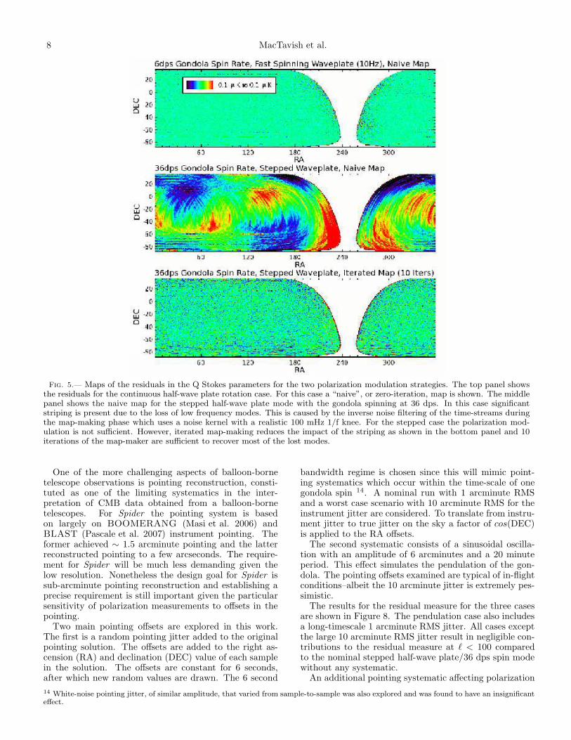
the stepped half-wave plate mode with the gondola spin-ning at 36 dps. In this case significant striping is presentdue to the loss of low frequency modes. These translate tolarge scale modes along the individual scans and result inthe striping obvious in the maps. Iterating the map-makerin this case reduces the effect of striping as the large scalemodes are recovered. After 10 iterations the striping issignificantly reduced as shown in the bottom panel of Fig-

ure 5. One possible way to reduce the computational loadof a map-making stage with many iterations is to spin thegondola faster to modulate the signal into higher frequen-cies.The power spectra for the BB residual measure (9) are

shown in Figure 6. The optimal solution is the continuoushalf-wave plate modulation scheme. This yields the lowestresidual compared to an r = 0.1 fiducial BB model. In thestepped the 36 dps, non-iterated case the residuals havethe same amplitude as the model on the largest scales.The residuals are reduced to < 1% levels for multipolesℓ < 100 when the map-maker is iterated 10 times. Thestepped 70 dps spin case with 10 iterations yields evensmaller residuals at the largest scales.Given the design and implementation advantages, the

simple stepped half-wave plate system appears a feasiblechoice for the Spider scan strategy, albeit with significantadditional computational costs 13. The remainder of thisSection is restricted to the stepped half-wave plate case. Inparticular the focus will be to probe whether any other sys-tematic effects invalidate this choice of modulation scheme.

4.2. Noise

To examine the impact of different 1/f profiles on thestepped mode residuals a number of different cases wererun.

• 36 dps gondola spin rate with 100 mHz detector 1/fknee.

• 36 dps gondola spin rate with 500 mHz 1/f knee.

• 110 dps gondola spin rate with 500 mHz 1/f knee.

The time-stream high-pass filter cut-off is kept at 10mHz in all cases. A comparison of BB signal residualsvarying the detector knee frequency is shown in Figure 7.Although simulations are signal only the time-streams areinverse noise filtered, as would be done for the real data.This reveals the impact of the detector noise characteris-tics in terms of the degradation of the polarization signalon the largest scales. The effect of a 500 mHz knee isclearly seen on the largest angular scales. Even for 10 it-erations of the map-maker the residuals are close to the20% level for this case. Increasing the spin rate to 110 dpsreduces the impact of the higher 1/f knee and approachesthe nominal 36 dps, 100 mHz knee case. A 500 mHz kneefrequency for the detectors and readout electronics is pes-simistic, but would not be catastrophic since polarizationmodulation can still be achieved by the faster spinninggondola. Spider ’s high frequency response is limited bythe noise and response time of the detectors the combina-tion of which sets the maximum gondola spin rate. With5 ms detectors, Spider can spin up to 110 dps before beingaffected by the detector noise and time constants. Thusfor the stepped half-wave plate case, the limit for the 1/fknee frequency is ∼500 mHz (for r = 0.1).

4.3. Pointing Systematics

13 A full exploration of faster, sub-optimal map-making algorithms is left for future work. In particular de-striping algorithms (seee.g. Ashdown et al. (2007)) may provide a much faster alternative although it is still not clear that these can be applied to a Spider ob-serving strategy and polarization sensitivity requirements.

8 MacTavish et al.

Fig. 5.— Maps of the residuals in the Q Stokes parameters for the two polarization modulation strategies. The top panel showsthe residuals for the continuous half-wave plate rotation case. For this case a “naive”, or zero-iteration, map is shown. The middlepanel shows the naive map for the stepped half-wave plate mode with the gondola spinning at 36 dps. In this case significantstriping is present due to the loss of low frequency modes. This is caused by the inverse noise filtering of the time-streams duringthe map-making phase which uses a noise kernel with a realistic 100 mHz 1/f knee. For the stepped case the polarization mod-ulation is not sufficient. However, iterated map-making reduces the impact of the striping as shown in the bottom panel and 10iterations of the map-maker are sufficient to recover most of the lost modes.

One of the more challenging aspects of balloon-bornetelescope observations is pointing reconstruction, consti-tuted as one of the limiting systematics in the inter-pretation of CMB data obtained from a balloon-bornetelescopes. For Spider the pointing system is basedon largely on BOOMERANG (Masi et al. 2006) andBLAST (Pascale et al. 2007) instrument pointing. Theformer achieved ∼ 1.5 arcminute pointing and the latterreconstructed pointing to a few arcseconds. The require-ment for Spider will be much less demanding given thelow resolution. Nonetheless the design goal for Spider issub-arcminute pointing reconstruction and establishing aprecise requirement is still important given the particularsensitivity of polarization measurements to offsets in thepointing.Two main pointing offsets are explored in this work.

The first is a random pointing jitter added to the originalpointing solution. The offsets are added to the right as-cension (RA) and declination (DEC) value of each samplein the solution. The offsets are constant for 6 seconds,after which new random values are drawn. The 6 second

bandwidth regime is chosen since this will mimic point-ing systematics which occur within the time-scale of onegondola spin 14. A nominal run with 1 arcminute RMSand a worst case scenario with 10 arcminute RMS for theinstrument jitter are considered. To translate from instru-ment jitter to true jitter on the sky a factor of cos(DEC)is applied to the RA offsets.The second systematic consists of a sinusoidal oscilla-

tion with an amplitude of 6 arcminutes and a 20 minuteperiod. This effect simulates the pendulation of the gon-dola. The pointing offsets examined are typical of in-flightconditions–albeit the 10 arcminute jitter is extremely pes-simistic.The results for the residual measure for the three cases

are shown in Figure 8. The pendulation case also includesa long-timescale 1 arcminute RMS jitter. All cases exceptthe large 10 arcminute RMS jitter result in negligible con-tributions to the residual measure at ℓ < 100 comparedto the nominal stepped half-wave plate/36 dps spin modewithout any systematic.An additional pointing systematic affecting polarization

14 White-noise pointing jitter, of similar amplitude, that varied from sample-to-sample was also explored and was found to have an insignificanteffect.

Spider Systematics 9

ℓ

ℓ(ℓ

+1) R

BBℓ / 2π

(µK

2)

Modulation Scheme

10 100

10-10

10-8

10-6

10-4

0.01

6dps Gondola/10Hz Fast WP, Naive map

36dps Gondola / 22.5˚ WP Step per Day, Naive Map

36dps Gondola / 22.5˚ WP Step per Day, 10 Iter Map

70dps Gondola / 22.5˚ WP Step per Day, 10 Iter Map

BB (r = 0.1)

Fig. 6.—Comparison of the BB residual from continuously spinning and stepped half-wave plate polarization modulation schemes.For the first case the half-wave plate spins continuously at 10 Hz while the gondola rotates at 6 dps. For the second case thehalf-wave plate is stepped by 22.5 degrees per day, while the gondola rotates at 36 dps or more. Operation in stepped half-waveplate mode, with the modulation provided by the spinning gondola, requires iterated map-making as the signal is not modulatedas far from the 1/f knee as in the continuously-rotating half-wave plate mode. 10 iterations of the map-maker is sufficient torecover the residual levels of the continuously-rotating half-wave plate case. Fewer iterations may be required if the gondola spinrate is even higher (70 dps case). The input BB spectrum for r = 0.1 is plotted for comparison.

10 MacTavish et al.

ℓ

ℓ(ℓ

+1) R

BBℓ/ 2π

(µK

2)

Noise Filter 1/f Knee

10 10010-9

10-8

10-7

10-6

10-5

10-4

0.001

0.01

0.1

36dps Gond/22.5˚ WP Step, 100mHz 1/f, 10iter Map

36dps Gond/22.5˚ WP Step, 500mHz 1/f, 10iter Map

110dps Gond/22.5˚ WP Step, 500mHz 1/f, 10iter Map

BB (r=0.1)

Fig. 7.— Impact of a higher 1/f detector knee on the BB residuals. Simulations are for signal only (with no noise) but time-streams are inverse noise filtered in the map-maker, giving a realistic estimate of modes that would be lost from 1/f effects in thereal data. With the higher knee frequency of 500 mHz the gondola spin rate must be increased to reduce the residuals to <2%levels over the target range of multipoles ℓ < 100. The maximum gondola spin rate of ∼ 110 dps is limited by the time responseand noise characteristics of the Spider detectors. The input BB spectrum for r = 0.1 is plotted for comparison.

ℓ

ℓ(ℓ

+1) R

BBℓ / 2π (µK

2)

Pointing Jitter

10 10010-10

10-9

10-8

10-7

10-6

10-5

10-4

0.001

0.01

0.1

Nominal Case

1arcmin/6sec Period RA/DEC Jitter

10 arcmin/6sec Period RA/DEC Jitter

1arcmin/1day Period RA/DEC Jitt+6arcmin/20min Period Pendulation

BB (r=0.1)

Fig. 8.— Three cases of pointing jitter. In the first two offsets are added to the RA and DEC with new offset values (withRMS amplitudes 1 arcminute or 10 arcminutes) every 6 seconds. In the third case, a sinusoidal oscillation is implemented withan amplitude of 6 arcminutes and a 20 minute period. This effect simulates the pendulation of the gondola. In addition for thelatter case, a long time scale (day period) 1 arcminute RMS jitter is added. Both types of pointing error, reconstruction error andin-flight pendulations, have negligible effects; a less than 1% effect even for the large 10 arcminute jitter.

Spider Systematics 11

ℓ

ℓ(ℓ

+1) R

BBℓ /2π

(µK

2)

Absolute and Relative Polarization Angle Offsets

10 10010-10

10-9

10-8

10-7

10-6

10-5

10-4

0.001

0.01

0.1

Nominal Case

0.5˚ RMS Offset, Channel by Channel

1.0˚ RMS Offset, Channel by Channel

0.25˚ Offset, All Channels Same

0.5˚ Offset, All Channels Same

1.0˚ Offset, All Channels Same

BB (r=0.1)

Fig. 9.— Residuals from absolute and relative offset of detector polarization angles. In the first two cases random 0.5 and 1degree RMS ψ errors are added to each detector. Residuals for these relative offsets are negligible. In the remaining cases thesame offset (0.25 degree, 0.5 degree and 1 degree) is applied to all channels, simulating an overall calibration error in the half-waveplate ψ angle. For a 1 degree absolute offset the effect is as high as 20%. The 0.5 degree offsets are required having only a fewpercent residual effect.

measurements is the requirement to reconstruct the angleψ (in equation 1) of the detector polarization relative tothe fixed, local Q and U frame of reference on the sky. Thesystematic can arise in two distinct ways. The first is arelative offset between the ψ angles of different detectors.The second is an overall offset in the focal plane referenceframe and the frame on the sky. The latter is generatedby any error in the calibration of the polarization angle ofthe instrument.Results from simulation of the ψ systematics are shown

in Figure 9. In the first two cases random 0.5 and 1 degreeRMS ψ errors are added to each detector. This simulatedfixed, random offsets in the relative polarization angles ofthe detectors. The results show the relative offsets con-tribute a comparable amount to the residuals as the nom-inal stepped mode case.In the remaining cases the same offset (0.25 degree, 0.5

degree and 1 degree) is applied to all channels. This sim-ulates an overall calibration error in the half-wave plateψ angle. The results show this systematic gives a muchlarger contribution to the residual. For a 1 degree abso-lute offset the effect is as high as 20%. The 0.5 degreeoffsets is required having only a few percent residual ef-fect. Again, simulations consider only 8 pairs in a singlecolumn or 16 detectors total. The RMS result for the fullfocal plane should average down as

√N , where N is the

number of detectors. This factor has not been applied tothe result. The calibration of the half-wave plate ψ angleswill be preformed pre-flight on the ground. The level ofsub-percent precision required is not a difficult measure-

ment and is made much easier by the compact optics andcorrespondingly close “far field” of Spider.Another systematic that is tested concerns pointing off-

sets of crossed pairs. This occurs if the E-field distributionis not identical at the feed, or if there are polarization de-pendent properties in the optics. For these simulations onedetector in a crossed pair (of the eight pairs) has a con-stant offset in RA and DEC of 1 or 4 arcminutes. Again,for the case of RA a factor of cos(DEC) is applied to theoffset and hence represents the true offset on the sky. ForSpider 40’ beams, the corresponding A-B amplitudes are3.6% and 14% for 1 arcminute and 4 arcminute offsets.Residuals for beam offsets are plotted in Figure 10. Theeffect is less than a few percent for ℓ < 80 for the largestoffset case.

4.4. Beam Systematics

The Spider antenna array and optics define highly sym-metric beams on the sky. The beam pattern shown inFigure 2 is the feed beam pattern. The beam on the skyis influenced by the telescope. While the Spider telescopeedge taper is modest, the beam on the sky will be moresymmetric than the feed pattern shown here. In particu-lar, the visibly large and asymmetric lobes above will notpropagate to the sky. The largest amplitude beam effectexpected comes from reflections or “ghosting” in the Spi-der optics. Ghosting is common in refractive optics andresults from unintended multiple reflections in the optics.The effect is a smaller amplitude beam image which is mir-rored with respect to the pixel position from the centre of

12 MacTavish et al.

ℓ

ℓ(ℓ

+1) RBBℓ / 2π (µK2)

Crossed-Pair Offsets

10 10010

-10

10-9

10-8

10-7

10-6

10-5

10-4

0.001

0.01

0.1

Nominal Case

1 arcmin RA/DEC Crossed Pair Offset Beams

4 arcmin RA/DEC Crossed Pair Offset Beams

BB (r=0.1)

Fig. 10.— For these simulations one detector in a crossed-pair (of the eight pairs) has a constant offset in RA and DEC of 1 or 4arcminutes. For Spider 40’ beams, the corresponding A-B amplitudes are 3.6% and 14% for 1 arcminute and 4 arcminute offsets.Residuals for beam offsets are plotted in Figure 10. The effect is less than a few percent for ℓ < 80 for the largest offset case.

ℓ

ℓ(ℓ

+1) RBBℓ / 2π (µK2)

Beam Ghosting

10 10010-10

10-9

10-8

10-7

10-6

10-5

10-4

0.001

0.01

0.1

Nominal Case

Ghosting 1% in TOD

Ghosting 5% in TOD

Ghosting 10% in TOD

BB (r=0.1)

Fig. 11.— The residuals from beam ghosting in the Spider optics. The ghosting is added in terms of a percent contamination tothe nominal time-stream. Final maps are then reconstructed assuming no reflection contamination with no attempt to correct forthe image distortion. A 10% contamination in the TOD yields a BB fractional residual as high as 20%. For 5% ghosting in theTOD this effect is already down by more than half and is negligible for 1% contamination in the TOD.

Spider Systematics 13

the focal plan.The ghosting is simulated by summing two time-streams

from two beams. One of the time-streams is constructedusing offset pointing from the ghost beam. The offsetpointing of the ghost is determined in instrument coor-dinates (elevation and azimuth), hence the ψ angle for theghost pointing is calculated appropriately as the final pro-jection of the orientation of a detector on the sky. Thesecond time-stream is constructed from the pointing fromthe nominal beam. The two time-streams are summedwith various weighting schemes depending on the ghostbeam contamination15.The residuals from beam ghosting are summarized in

Figure 11. For each case the ghosting effect is added inthe time-stream in terms of a percent contamination addedto the nominal time-stream. Final maps are then recon-structed assuming no reflection contamination; there is noattempt to correct for the image distortion. With 10%contamination in the TOD the effect in the BB residual isas much as 20%. For 5% ghosting in the TOD this effect isalready down by more than half and is negligible for 1% inthe TOD. Since simulations are done only for a single row(of 8 pairs of detectors) the distance between the originaland ghost images is, on average, smaller for this row thanfor any other. It is therefore worth noting that the fullfocal plane may show a larger effect than that simulatedhere.

4.5. Calibration Drift

Diurnal variations in the detector sensitivity will occurdue to altitude-induced changes in background loading.These sensitivity changes will be tracked using 4K semi-conductor emitters (fired intermittently) similar to thoseused in BOOMERANG flights. For BOOMERANG2003 flight, the gain drift for each individual detector wasdetermined by the uncertainty on an individual calibrationpulse and was measured to be 0.05%. With an improvedversion of the calibration lamp and Spider ’s higher sensi-tivity, the expected uncertainty is ∼ 0.01%. Knowledge ofthe detector model (determined in pre-flight testing) willalso allow the calculation of the sensitivity for any givenoperating point.Figure 12 shows the effect of uncorrected calibration

drift. Two cases are considered. For the first case thecalibration drift is the same for all detectors, changing ona diurnal timescale with a maximum amplitude of 3%. Forthis case the resulting residual is small; less than a percentat all scales.For the second case the gain drift for all detectors are

of the same amplitude and with a 24 hour period, buteach of the 16 detectors have a gain drift with a differentphase. Thus at any given time sample the calibration fac-tor within a pair of detectors will be different. Simulationsconsider only 8 pairs in a single column or 16 detectors to-tal. Again, the RMS result for the full focal plane shouldaverage down as

√N , where N is the number of detec-

tors. For this case a factor of√16/

√1024 (assuming 1024

CMB science channels) has been applied to each residualresult. The BB fractional residual is as much as 50% for again drift amplitude of 3%. For a 0.5% amplitude drift theresidual drops below the 5% level. As with all simulationsin this work there has been no attempt to correct for thegain systematic. For BOOMERANG 2003, the final rel-ative calibration uncertainty was 0.4% (Masi et al. 2006).Spider is expected to achieve an uncertainty of 0.1% or lesswhich will be more than adequate to meet science goals.

5. conclusions

The results from Section 4 are summarized in terms ofexperimental specifications in Table 2. While results areSpider -specific the order of magnitude of various effectscan be translated to other CMB polarization experiments.The RMS B-mode signal for r = 0.1 is roughly 10000 nK2

(∼1436 nK2 at ℓ = 8 and ∼7379 nK2 at ℓ = 80), andscales linearly with r. Experimental specifications are setby limiting the allowed systematic residual level to a factorof ∼ 10 smaller than the B-mode signal for r = 0.01.While the simulations were signal-only the impact of

large low frequency detector noise (1/f noise) is reflectedin the large scale degradation of the B-mode signal for thestepped half-wave plate mode of operation. Rapid, contin-uous half-wave plate modulation mitigates this effect en-tirely. Rapid, continuous gondola rotation also works butonly with iterative map-making which accurately recoversthe larger scale signal.It is important to note that the effects studied in Sec-

tions 4.1 and Sections 4.2 (naive versus iterated maps,spinning more slowly, stepping half-wave plate versusspinning half-wave plate) will degrade the signal-to-noiseachieved on the bandpowers. These effects differ from thesystematics studied in Section 4.3 to Section 4.5 (point-ing reconstruction errors, polarization angle uncertainty,uncorrected ghosting, uncorrected gain drifts) which willultimately bias the final result. The requirements on thebiasing effects are more difficult treat than the signal-to-noise issues.The impact of systematics on B-mode polarimeter ex-

periments is also discussed in Hu et al. (2003) and morerecently O’Dea et al. (2007), where analytical methodsare used for calculating the B-mode spectrum bias. Theresults are useful for setting experimental “benchmark pa-rameters” at the very earliest phases of instrument design.This work goes a step further by considering the impactof systematics in the map/time-domain; A necessary stepin the evolution of an experiment which aims to measurethe tiny primordial, gravity wave signal.

This research used the McKenzie cluster at CITA,funded by the Canada Foundation for Innovation. Someof the results in this paper have been derived using theHEALPix package [Gorski et al. (2005)] as well as theFFTW package [Frigo & Johnson (2005)].

15 In order to completely model the polarization of the ghost, a half-wave plate angle dependency should be included in the ratio of ghostamplitude to main-beam response. This is not done here but is left for future work.

14 MacTavish et al.

ℓ

ℓ(ℓ

+1) RBBℓ / 2π (µK2)

Calibration Drift

10 10010

-10

10-9

10-8

10-7

10-6

10-5

10-4

0.001

0.01

0.1

Nominal Case

3% Calibration Dirurnal Drift--All Detectors in Phase

0.5% Calibration Dirurnal Drift--Out of Phase

3% Calibration Dirurnal Drift--Out of Phase

BB (r=0.1)

Fig. 12.— The effect of uncorrected calibration drift. In the first case the calibration drift is the same for all detectors, changingon a diurnal timescale with a maximum amplitude of 3%. For the second case the gain drift for all detectors are of the sameamplitude and diurnal but out of phase. For this case, the BB fractional residual is as much as 50% for a gain drift amplitudeof 3% and drops below 5% for a 0.5% amplitude gain drift. Simulations consider only 8 pairs in a single column or 16 detectorstotal. The RMS result for the full focal plane will average down as

√N , where N is the number of detectors. For the second case

(out of phase gain drifts) a factor of√16/

√1024 (assuming 1024 CMB science channels) has been applied to each residual result.

Systematic Experimental Spec. Comments

Receiver for 110dps1/f knee < 200 mHz gondola spinReceiver for 36dps1/f knee < 100 mHz gondola spinPointing sufficient forJitter < 10′ ℓ < 50

AbsolutePol. Angle Offset < 0.25 deg.

RelativePol. Angle Offset < 1 deg.Knowledge of sufficient for

Beam Centroids < 1′ ℓ < 30Optical % TODGhosting < 2% contaminationCalibration

Drift < 3.0% in phaseCalibration

Drift < 0.1% out of phase

Table 2

Summary of experimental specifications based on simulation results. Realistic-amplitude, time-varying systematics are injectedin the simulated time streams. Maps are reconstructed without any attempt to correct for the systematic errors. Experimentalspecifications are set by limiting the allowed systematic residual level to a factor of ∼ 10 smaller than the B-mode signal for

r = 0.01. The nominal operating mode is a 36 dps gondola spin rate, with the half-wave plate stepping 22.5◦ once per day, with10 iterations (sufficient to recover the residual levels of the continuously-rotating half-wave plate case) of the map-maker, a

Jacobi iterative solver (Jones et al. 2007).

Spider Systematics 15

REFERENCES

Adams, F., Bond, J. R., Freese, K., Frieman, J., & Olinto, A. 1993,Physical Review D, 47, 426

Ade, P. et al. 2007, ArXiv e-prints, 705Ashdown, M. A. J., Baccigalupi, C., Balbi, A., Bartlett, J. G.,

Borrill, J., Cantalupo, C., de Gasperis, G., Gorski, K. M., Hivon,E., Keihanen, E., Kurki-Suonio, H., Lawrence, C. R., Natoli, P.,Poutanen, T., Prunet, S., Reinecke, M., Stompor, R., Wandelt, B.,& The Planck CTP Working Group. 2007, A&A, 467, 761

Battistelli, E. et al. 2007, Journal of Low Temperature Physics,Proceedings of the 12th international workshop on LowTemperature Detectors

Bock, J., Church, S., Devlin, M., Hinshaw, G., Lange, A., Lee, A.,Page, L., Partridge, B., Ruhl, J., Tegmark, M., Timbie, P., Weiss,R., Winstein, B., & Zaldarriaga, M. 2006, ArXiv Astrophysics e-prints

Bunn, E. F., Zaldarriaga, M., Tegmark, M., & de Oliveira-Costa, A.2003, Phys. Rev. D, 67, 023501

Chervenak, J. A., Irwin, K. D., Grossman, E. N., Martinis, J. M.,Reintsema, C. D., & Huber, M. E. 1999, Applied Physics Letters,74, 4043

de Korte, P. A. J., Beyer, J., Deiker, S., Hilton, G. C., Irwin, K. D.,Macintosh, M., Nam, S. W., Reintsema, C. D., Vale, L. R., &Huber, M. E. 2003, Review of Scientific Instruments, 74, 3807

Frigo, M. & Johnson, S. G. 2005, Proceedings of the IEEE, 93, 216Goldin, A., Bock, J. J., Hunt, C., Lange, A. E., Leduc, H., Vayonakis,

A., & Zmuidzinas, J. 2002, Low Temperature Detectors, 605, 251Gorski, K. M., Hivon, E., Banday, A. J., Wandelt, B. D., Hansen,

F. K., Reinecke, M., & Bartelmann, M. 2005, ApJ, 622, 759Harry, G. M., Fritschel, P., Shaddock, D. A., Folkner, W., & Phinney,

E. S. 2006, Classical and Quantum Gravity, 23, 1Hedman, M. M., Barkats, D., Gundersen, J. O., McMahon, J. J.,

Staggs, S. T., & Winstein, B. 2002, ApJ, 573, L73Hivon, E., Gorski, K. M., Netterfield, C. B., Crill, B. P., Prunet, S.,

& Hansen, F. 2002, ApJ, 567, 2Holland, W., MacIntosh, M., Fairley, A., Kelly, D., Montgomery, D.,

Gostick, D., Atad-Ettedgui, E., Ellis, M., Robson, I., Hollister, M.,Woodcraft, A., Ade, P., Walker, I., Irwin, K., Hilton, G., Duncan,W., Reintsema, C., Walton, A., Parkes, W., Dunare, C., Fich, M.,Kycia, J., Halpern, M., Scott, D., Gibb, A., Molnar, J., Chapin,E., Bintley, D., Craig, S., Chylek, T., Jenness, T., Economou,F., & Davis, G. 2006, in Presented at the Society of Photo-Optical Instrumentation Engineers (SPIE) Conference, Vol. 6275,Millimeter and Submillimeter Detectors and Instrumentation forAstronomy III. Edited by Zmuidzinas, Jonas; Holland, Wayne S.;Withington, Stafford; Duncan, William D.. Proceedings of theSPIE, Volume 6275, pp. 62751E (2006).

Hu, W., Hedman, M. M., & Zaldarriaga, M. 2003, Phys. Rev. D, 67,043004

Irwin, K. D., Audley, M. D., Beall, J. A., Beyer, J., Deiker, S.,Doriese, W., Duncan, W., Hilton, G. C., Holland, W., Reintsema,C. D., Ullom, J. N., Vale, L. R., & Xu, Y. 2004, NuclearInstruments and Methods in Physics Research A, 520, 544

Jones, W. C., Montroy, T. E., Crill, B. P., Contaldi, C. R., Kisner,T. S., Lange, A. E., MacTavish, C. J., Netterfield, C. B., & Ruhl,J. E. 2007, A&A, 470, 771

Jones, W. C. et al. 2006, Astrophys. J., 647, 823Kallosh, R. 2007, ArXiv High Energy Physics - Theory e-printsKeating, B. G., Ade, P. A. R., Bock, J. J., Hivon, E., Holzapfel, W. L.,

Lange, A. E., Nguyen, H., & Yoon, K. W. 2003, in Presented atthe Society of Photo-Optical Instrumentation Engineers (SPIE)Conference, Vol. 4843, Polarimetry in Astronomy. Edited bySilvano Fineschi . Proceedings of the SPIE, Volume 4843, pp. 284-295 (2003)., ed. S. Fineschi, 284–295

Kogut, A., Dunkley, J., Bennett, C. L., Dore, O., Gold, B., Halpern,M., Hinshaw, G., Jarosik, N., Komatsu, E., Nolta, M. R., Odegard,N., Page, L., Spergel, D. N., Tucker, G. S., Weiland, J. L., Wollack,E., & Wright, E. L. 2007, ArXiv e-prints, 704

Kovac, J. et al. 2002, Nature, 420, 772Kuo, C. L., Bock, J. J., Chattopadthyay, G., Goldin, A., Golwala,

S., Holmes, W., Irwin, K., Kenyon, M., Lange, A. E., LeDuc,H. G., Rossinot, P., Vayonakis, A., Wang, G., Yun, M., &Zmuidzinas, J. 2006, in Presented at the Society of Photo-Optical Instrumentation Engineers (SPIE) Conference, Vol. 6275,Millimeter and Submillimeter Detectors and Instrumentation forAstronomy III. Edited by Zmuidzinas, Jonas; Holland, Wayne S.;Withington, Stafford; Duncan, William D.. Proceedings of theSPIE, Volume 6275, pp. 62751M (2006).

Lewis, A., Challinor, A., & Turok, N. 2002, Phys. Rev. D, 65, 023505Linde, A. 1994, Phys. Rev. D, 49, 748Linde, A., Mukhanov, V., & Sasaki, M. 2005, Journal of Cosmology

and Astro-Particle Physics, 10, 2Linde, A. D. 1983, Physics Letters B, 129, 177MacTavish, C. J. et al. 2006, Astrophys. J., 647, 799Masi, S. et al. 2006, A&A, 458, 687Montroy, T. E. et al. 2006a, Astrophys. J., 647, 813Montroy, T. E. et al. 2006b, in Presented at the Society of Photo-

Optical Instrumentation Engineers (SPIE) Conference, Vol. 6267,Ground-based and Airborne Telescopes. Edited by Stepp, LarryM.. Proceedings of the SPIE, Volume 6267, pp. 62670R (2006).

O’Dea, D., Challinor, A., & Johnson, B. R. 2007, MNRAS, 376, 1767Page, L., Hinshaw, G., Komatsu, E., Nolta, M. R., Spergel, D. N.,

Bennett, C. L., Barnes, C., Bean, R., Dore, O., Dunkley, J.,Halpern, M., Hill, R. S., Jarosik, N., Kogut, A., Limon, M., Meyer,S. S., Odegard, N., Peiris, H. V., Tucker, G. S., Verde, L., Weiland,J. L., Wollack, E., & Wright, E. L. 2007, ApJS, 170, 335

Pascale, E. et al. 2007, Submitted to ApJPhinney, E. S. et al. 2004, NASA Mission Concept StudyPiacentini, F. et al. 2006, Astrophys. J., 647, 833Readhead, A. C. S. et al. 2004, Science, 306, 836Reintsema, C. D., Beyer, J., Nam, S. W., Deiker, S., Hilton, G. C.,

Irwin, K., Martinis, J., Ullom, J., Vale, L. R., & Macintosh, M.2003, Review of Scientific Instruments, 74, 4500

Schlegel, D. J., Finkbeiner, D. P., & Davis, M. 1998, ApJ, 500, 525Spergel, D. N. et al. 2007, ApJS, 170, 377Szapudi, I., Prunet, S., & Colombi, S. 2001, ArXiv Astrophysics e-

prints