Embed Size (px)
Citation preview
Submitted to Statistical Science
Models as Approximations —A Conspiracy of Random Predictorsand Model Violations Against ClassicalInference in RegressionAndreas Buja∗,†,‡, Richard Berk‡, Lawrence Brown∗,‡, Edward George‡, Emil Pitkin∗,‡,Mikhail Traskin§ , Linda Zhao∗,‡ and Kai Zhang∗,¶
Wharton – University of Pennsylvania‡ and Amazon.com§ and UNC at Chapel Hill¶
Dedicated to Halbert White (†2012)
Abstract.
We review and interpret the early insights of Halbert White who over
thirty years ago inaugurated a form of statistical inference for regression
models that is asymptotically correct even under “model misspecifica-
tion,” that is, under the assumption that models are approximations
rather than generative truths. This form of inference, which is perva-
sive in econometrics, relies on the “sandwich estimator” of standard
error. Whereas linear models theory in statistics assumes models to
be true and predictors to be fixed, White’s theory permits models to
be approximate and predictors to be random. Careful reading of his
work shows that the deepest consequences for statistical inference arise
from a synergy — a “conspiracy” — of nonlinearity and randomness of
the predictors which invalidates the ancillarity argument that justifies
conditioning on the predictors when they are random. An asymptotic
comparison of standard error estimates from linear models theory and
White’s asymptotic theory shows that discrepancies between them can
be of arbitrary magnitude. In practice, when there exist discrepancies,
linear models theory tends to be too liberal but occasionally it can be
too conservative as well. A valid alternative to the sandwich estimator is
provided by the “pairs bootstrap”; in fact, the sandwich estimator can
be shown to be a limiting case of the pairs bootstrap. Finally we give
Statistics Department, The Wharton School, University of Pennsylvania, 400 Jon M. Huntsman
Hall, 3730 Walnut Street, Philadelphia, PA 19104-6340 (e-mail: [email protected]).
Amazon.com. Dept. of Statistics & Operations Research, 306 Hanes Hall, CB#3260, The
University of North Carolina at Chapel Hill, Chapel Hill, NC 27599-3260.∗Supported in part by NSF Grant DMS-10-07657.†Supported in part by NSF Grant DMS-10-07689.
1imsart-sts ver. 2014/07/30 file: Buja_et_al_A_Conspiracy.tex date: August 19, 2014
2 A. BUJA ET AL.
meaning to regression slopes when the linear model is an approxima-
tion rather than a truth. — We limit ourselves to linear LS regression,
but many qualitative insights hold for most forms of regression.
AMS 2000 subject classifications: Primary 62J05, 62J20, 62F40; sec-
ondary 62F35, 62A10.
Key words and phrases: Ancillarity of predictors, First and second order
incorrect models, Model misspecification, Misspecification tests, Econo-metrics, Sandwich estimator of standard error, Pairs bootstrap.
1. INTRODUCTION
The classical Gaussian linear model reads as follows:
(1) y = Xβ + ε , ε ∼ N (0N , σ2IN×N ) (y, ε ∈ IRN , X ∈ IRN×(p+1), β ∈ IRp+1).
Two aspects will be important: (1) the model is assumed correct, including linearity of the response
means in the predictors and independence, homoskedasticity and Gaussianity of the errors; (2) the
predictors are treated as known constants, even when they are as random as the response. Statisticians
have long enjoyed the fruits that can be harvested from this model and they have taught it as funda-
mental at all levels of statistical education. Curiously little known to many statisticians is the fact that
a different framework is adopted and a different statistical education is taking place in the parallel
universe of econometrics. For over three decades, starting with Halbert White’s (1980a,b;1981;1982)
seminal articles, econometricians have used multiple linear regression without making the many as-
sumptions of classical linear models theory. While statisticians use assumption-laden exact finite
sample inference, econometricians use assumption-lean asymptotic inference based on the
so-called “sandwich estimator” of standard error. In our experience most statisticians have heard
of the sandwich estimator but do not know its purpose, use, and underlying theory. A first goal
of the present exposition is therefore to convey an understanding of an assumption-lean framework
in a language that is intelligible to statisticians. The approach is to interpret linear regression in
a semi-parametric fashion as extraction of a parametric linear part of a general nonlinear response
surface. The modeling assumptions can then be reduced to i.i.d. sampling from largely arbitrary joint
( ~X, Y ) distributions that satisfy a few moment conditions. In this assumption-lean framework the
sandwich estimator produces asymptotically correct standard errors.
A second goal of this exposition is to connect the assumption-lean framework to a form of sta-
tistical inference in linear models that is known to statisticians but appreciated by few: the “pairs
bootstrap.” As the name indicates, the pairs bootstrap consists of resampling pairs (~xi, yi), in con-
trast to the “residual bootstrap” which resamples residuals ri. Among the two, the pairs bootstrap is
the less promoted even though asymptotic theory exists to justify both under different assumptions
(see, for example, Freedman 1981, Mammen 1993). It is intuitively clear that the pairs bootstrap
can be asymptotically justified in the assumption-lean framework, and for this reason it produces
standard error estimates that solve the same problem as the sandwich estimator. Indeed, we estab-
lish a connection that shows the sandwich estimator to be the asymptotic limit of the M -of-N pairs
bootstrap when M → ∞. We will use the general term “assumption-lean estimator” to refer to
either the sandwich estimator or the pairs bootstrap estimator of standard error.
imsart-sts ver. 2014/07/30 file: Buja_et_al_A_Conspiracy.tex date: August 19, 2014
MODELS AS APPROXIMATIONS 3
A third goal of this article is to theoretically and practically compare the assumption-lean estima-
tors with the linear models estimator. We define a ratio of asymptotic variances — “RAV ” for short
— that describes the discrepancies between the two types of standard error estimators in the asymp-
totic limit. If there exists a discrepancy, RAV 6= 1, it will be assumption-lean estimators (sandwich
or pairs bootstrap) that are asymptotically correct, and the linear models estimator is then indeed
asymptotically incorrect. If RAV 6= 1, there exist deviations from the linear model in the form of
nonlinearities and/or heteroskedasticities. If RAV = 1, the linear models estimator is asymptotically
correct, but this does not imply that the linear model is correct, the reason being that nonlinearities
and heteroskedasticities can combine to produce a coincidentally correct size for the linear models
estimator. Importantly, the RAV is specific to each regression coefficient because the magnitudes of
the discrepancies can vary from coefficient to coefficient in the same model.
A fourth goal is to estimate the RAV for use as a test statistic. We derive an asymptotic null
distribution to test the presence of model violations that invalidate the classical standard error of
a specific coefficient. While the result can be called a “misspecification test” in the tradition of
econometrics, it is more usefully viewed as guidance to the better standard error. The sandwich
estimator comes with a cost — vastly increased non-robustness — which makes it desirable to use
the linear models standard error when possible. However, a procedure that chooses the type of
standard error depending on the outcome of a pre-test raises new performance issues that require
future research. (Simpler is Angrist and Pischke’s proposal (2009) to choose the larger of the two
standard errors; their procedure forfeits the possibility of detecting the classical standard error as
too conservative. MacKinnon and White (1985) on the other hand recommend using a sandwich
estimator even if no misspecification is detected.)
A fifth and final goal of this article is to propose answers to questions and objections that would
be natural to statisticians who hold the following tenets:
1. Models need to be “correct” for inference to be meaningful. The implication is that assumption-
lean approaches are misguided because inference in “misspecified models” are meaningless.
2. Predictors in regression models should or can be treated as fixed even if they are random.
The implication is that inference which treats predictors as random is unprincipled or at best
superfluous.
A strong proponent of the first tenet is the late David Freedman (2006). While his insistence on
intellectual honesty and rigor is admirable, we will counterargue based on White (1980a,b; 1981;
1982) that inference under misspecification can be meaningful and rigorous. Abandoning the negative
rhetoric of “misspecification”, we adopt the following alternative view:
1. Models are always approximations, not truths (Box 1979; Cox 1995).
2. If models are approximations, regression slopes still have meaningful interpretations.
3. If models are approximations, it is prudent to use inference that is less dependent on model
correctness.
In fact, neither the second nor the third point depends on the degree of approximation: meaningful
interpretation and valid inference can be provided for regression slopes whether models are good or
bad approximations. (This is of course not to say that every regression analysis is meaningful.)
The second tenet above, conditionality on predictors, has proponents to various degrees. More
imsart-sts ver. 2014/07/30 file: Buja_et_al_A_Conspiracy.tex date: August 19, 2014
4 A. BUJA ET AL.
forceful ones hold that conditioning on the predictors is a necessary consequence of the ancillarity
principle; others hold that the principle confers license, not a mandate. The ancillarity principle
says in simplified terms that valid inference results from conditioning on statistics whose distribu-
tion does not involve the parameters of interest. When the predictors in a regression are random,
their distribution is ancillary for the regression parameters, hence conditioning on the predictors is
necessary or at least permitted. This argument, however, fails when the parametric model is only
an approximation and the predictors are random. It will be seen that under these circumstances the
population slopes do depend on the predictor distribution which is hence not ancillary. This effect
does not exist when the conditional mean of the response is a linear function of the predictors or the
predictors are truly nonrandom.
This article continuous as follows: Section 2 illustrates discrepancies between standard error esti-
mates with real data examples. Section 3 sets up the semi-parametric population framework in which
LS approximation extracts a parametric linear component. Section 4 shows how nonlinear conditional
expectations invalidate ancillarity of the predictor distribution. Section 5 derives a decomposition of
asymptotic variance of LS estimates into contributions from noise and from nonlinearity, and central
limit theorems associated with the decomposition. Section 6 introduces the simplest version of the
sandwich estimator of standard error and shows how it is a limiting case of the M -of-N pairs boot-
strap. Section 7 expresses parameters, estimates, asymptotic variances and CLTs in the language
of predictor adjustment, which is critical in order to arrive at expressions that speak to individual
predictors in a transparent fashion. In Section 8 the language of adjustment allows us to define the
RAV , that is, the ratio of proper (assumption-lean) and improper (linear models-based) asymptotic
variances and to analyze conditions under which linear models theory yields standard errors that
are too liberal (often) or too conservative (less often). Section 9 turns the RAV into a simple test
statistic with an asymptotically normal null distribution under “well-specification”. The penultimate
Section 10 proposes an answer to the question of what the meaning of regression coefficients is when
the linear model is an approximation rather than a generative truth. The final Section 11 has a brief
summary and ends with a pointer to problematic aspects of the sandwich estimator. Throughout
we use precise notation for clarity. The notation may give the impression of a technical article, but
all technical results are elementary and all limit theorems are stated informally without regularity
conditions.
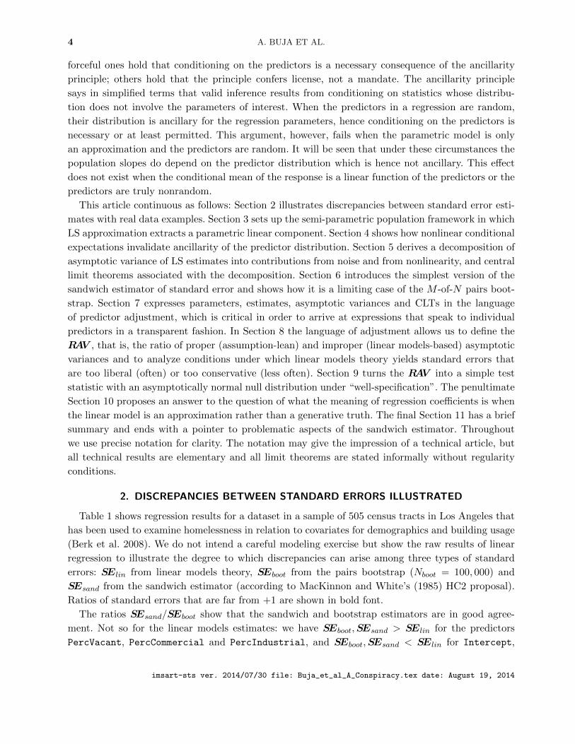
2. DISCREPANCIES BETWEEN STANDARD ERRORS ILLUSTRATED
Table 1 shows regression results for a dataset in a sample of 505 census tracts in Los Angeles that
has been used to examine homelessness in relation to covariates for demographics and building usage
(Berk et al. 2008). We do not intend a careful modeling exercise but show the raw results of linear
regression to illustrate the degree to which discrepancies can arise among three types of standard
errors: SElin from linear models theory, SEboot from the pairs bootstrap (Nboot = 100, 000) and
SEsand from the sandwich estimator (according to MacKinnon and White’s (1985) HC2 proposal).
Ratios of standard errors that are far from +1 are shown in bold font.
The ratios SEsand/SEboot show that the sandwich and bootstrap estimators are in good agree-
ment. Not so for the linear models estimates: we have SEboot,SEsand > SElin for the predictors
PercVacant, PercCommercial and PercIndustrial, and SEboot,SEsand < SElin for Intercept,
imsart-sts ver. 2014/07/30 file: Buja_et_al_A_Conspiracy.tex date: August 19, 2014
MODELS AS APPROXIMATIONS 5
βj SElin SEboot SEsandSEbootSElin
SEsandSElin
SEsandSEboot
tlin tboot tsand
Intercept 0.760 22.767 16.505 16.209 0.726 0.712 0.981 0.033 0.046 0.047
MedianInc ($K) -0.183 0.187 0.114 0.108 0.610 0.576 0.944 -0.977 -1.601 -1.696
PercVacant 4.629 0.901 1.385 1.363 1.531 1.513 0.988 5.140 3.341 3.396
PercMinority 0.123 0.176 0.165 0.164 0.937 0.932 0.995 0.701 0.748 0.752
PercResidential -0.050 0.171 0.112 0.111 0.653 0.646 0.988 -0.292 -0.446 -0.453
PercCommercial 0.737 0.273 0.390 0.397 1.438 1.454 1.011 2.700 1.892 1.857
PercIndustrial 0.905 0.321 0.577 0.592 1.801 1.843 1.023 2.818 1.570 1.529
Table 1Comparison of Standard Errors for the LA Homeless Data.
MedianInc ($1000), PercResidential. Only for PercMinority is SElin off by less than 10% from
SEboot and SEsand. The discrepancies affect outcomes of some of the t-tests: Under linear mod-
els theory the predictors PercCommercial and PercIndustrial have commanding t-values of 2.700
and 2.818, respectively, which are reduced to unconvincing values below 1.9 and 1.6, respectively,
if the pairs bootstrap or the sandwich estimator are used. On the other hand, for MedianInc ($K)
the t-value −0.977 from linear models theory becomes borderline significant with the bootstrap or
sandwich estimator if the plausible one-sided alternative with negative sign is used.
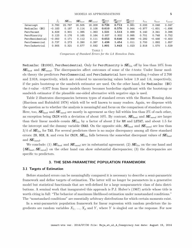
Table 2 illustrates discrepancies between types of standard errors with the Boston Housing data
(Harrison and Rubinfeld 1978) which will be well known to many readers. Again, we dispense with
the question as to whether the analysis is meaningful and focus on the comparison of standard errors.
Here, too, SEboot and SEsand are mostly in agreement as they fall within less than 2% of each other,
an exception being CRIM with a deviation of about 10%. By contrast, SEboot and SEsand are larger
than their linear models cousin SElin by a factor of about 2 for RM and LSTAT, and about 1.5 for
the intercept and the dummy variable CHAS. On the opposite side, SEboot and SEsand are less than
3/4 of SElin for TAX. For several predictors there is no major discrepancy among all three standard
errors: ZN, NOX, B, and even for CRIM, SElin falls between the somewhat discrepant values of SEboot
and SEsand.
We conclude: (1) SEboot and SEsand are in substantial agreement; (2) SElin on the one hand and
{SEboot,SEsand} on the other hand can show substantial discrepancies; (3) the discrepancies are
specific to predictors.
3. THE SEMI-PARAMETRIC POPULATION FRAMEWORK
3.1 Targets of Estimation
Before standard errors can be meaningfully compared it is necessary to describe a semi-parametric
framework and define targets of estimation. The latter will no longer be parameters in a generative
model but statistical functionals that are well-defined for a large nonparametric class of data distri-
butions. A seminal work that inaugurated this approach is P.J. Huber’s (1967) article whose title is
worth citing in full: “The behavior of maximum likelihood estimation under nonstandard conditions.”
The “nonstandard conditions” are essentially arbitrary distributions for which certain moments exist.
In a semi-parametric population framework for linear regression with random predictors the in-
gredients are random variables X1, ..., Xp and Y , where Y is singled out as the response. For now
imsart-sts ver. 2014/07/30 file: Buja_et_al_A_Conspiracy.tex date: August 19, 2014
6 A. BUJA ET AL.
βj SElin SEboot SEsandSEbootSElin
SEsandSElin
SEsandSEboot
tlin tboot tsand
(Intercept) 36.459 5.103 8.038 8.145 1.575 1.596 1.013 7.144 4.536 4.477
CRIM -0.108 0.033 0.035 0.031 1.055 0.945 0.896 -3.287 -3.115 -3.478
ZN 0.046 0.014 0.014 0.014 1.005 1.011 1.006 3.382 3.364 3.345
INDUS 0.021 0.061 0.051 0.051 0.832 0.823 0.990 0.334 0.402 0.406
CHAS 2.687 0.862 1.307 1.310 1.517 1.521 1.003 3.118 2.056 2.051
NOX -17.767 3.820 3.834 3.827 1.004 1.002 0.998 -4.651 -4.634 -4.643
RM 3.810 0.418 0.848 0.861 2.030 2.060 1.015 9.116 4.490 4.426
AGE 0.001 0.013 0.016 0.017 1.238 1.263 1.020 0.052 0.042 0.042
DIS -1.476 0.199 0.214 0.217 1.075 1.086 1.010 -7.398 -6.882 -6.812
RAD 0.306 0.066 0.063 0.062 0.949 0.940 0.990 4.613 4.858 4.908
TAX -0.012 0.004 0.003 0.003 0.736 0.723 0.981 -3.280 -4.454 -4.540
PTRATIO -0.953 0.131 0.118 0.118 0.899 0.904 1.005 -7.283 -8.104 -8.060
B 0.009 0.003 0.003 0.003 1.026 1.009 0.984 3.467 3.379 3.435
LSTAT -0.525 0.051 0.100 0.101 1.980 1.999 1.010 -10.347 -5.227 -5.176Table 2
Comparison of Standard Errors for the Boston Housing Data.
the only assumption is that these variables have a joint distribution
P = P (dy,dx1, ...,dxp)
whose second moments exist and whose predictors have a full rank covariance matrix. We write
~X = (1, X1, ..., Xp)T .
for the column random vector consisting of the predictor variables, with a constant 1 prepended
to accommodate an intercept term. Values of the random vector ~X will be denoted by lower case
~x = (1, x1, ..., xp)T . We write any function f(X1, ..., Xp) of the predictors equivalently as f( ~X) as
the prepended constant 1 is irrelevant. Correspondingly we also use the notations
(2) P = P (dy,d~x), P (d~x), P (dy | ~x) and P = PY, ~X
, P ~X, P
Y | ~X ,
for the joint distribution of (Y, ~X), the marginal distribution of ~X, and the conditional distribu-
tion of Y given ~X, respectively. Nonsingularity of the predictor covariance matrix is equivalent to
nonsingularity of the cross-moment matrix E[ ~X ~XT
].
Among functions of the predictors, an important one is the best L2(P ) approximation to the
response Y , which is the conditional expectation of Y given ~X:
(3) µ( ~X) := argminf( ~X)∈L2(P )
E[(Y − f( ~X))2] = E[Y | ~X ] .
This is also called the “response surface.” Importantly we do not assume that µ( ~X) is linear in ~X.
Among linear functions l( ~X) = βT ~X, one stands out as the best linear L2(P ) approximation or
the population LS linear approximation to Y :
(4) β(P ) := argminβ∈IRp+1 E[(Y − βT ~X)2] = E[ ~X ~XT
]−1E[ ~XY ] .
The right most expression follows from the normal equations E[ ~X ~XT
]β−E[ ~XY ] = 0 that are the
stationarity conditions for minimizing the population LS criterion E[(Y −βT ~X)2] = −2βTE[ ~XY ]+
βTE[ ~X ~XT
]β + const.
imsart-sts ver. 2014/07/30 file: Buja_et_al_A_Conspiracy.tex date: August 19, 2014
MODELS AS APPROXIMATIONS 7
x
y
µ(x)βTx
●
●
●y
ε
η
δ
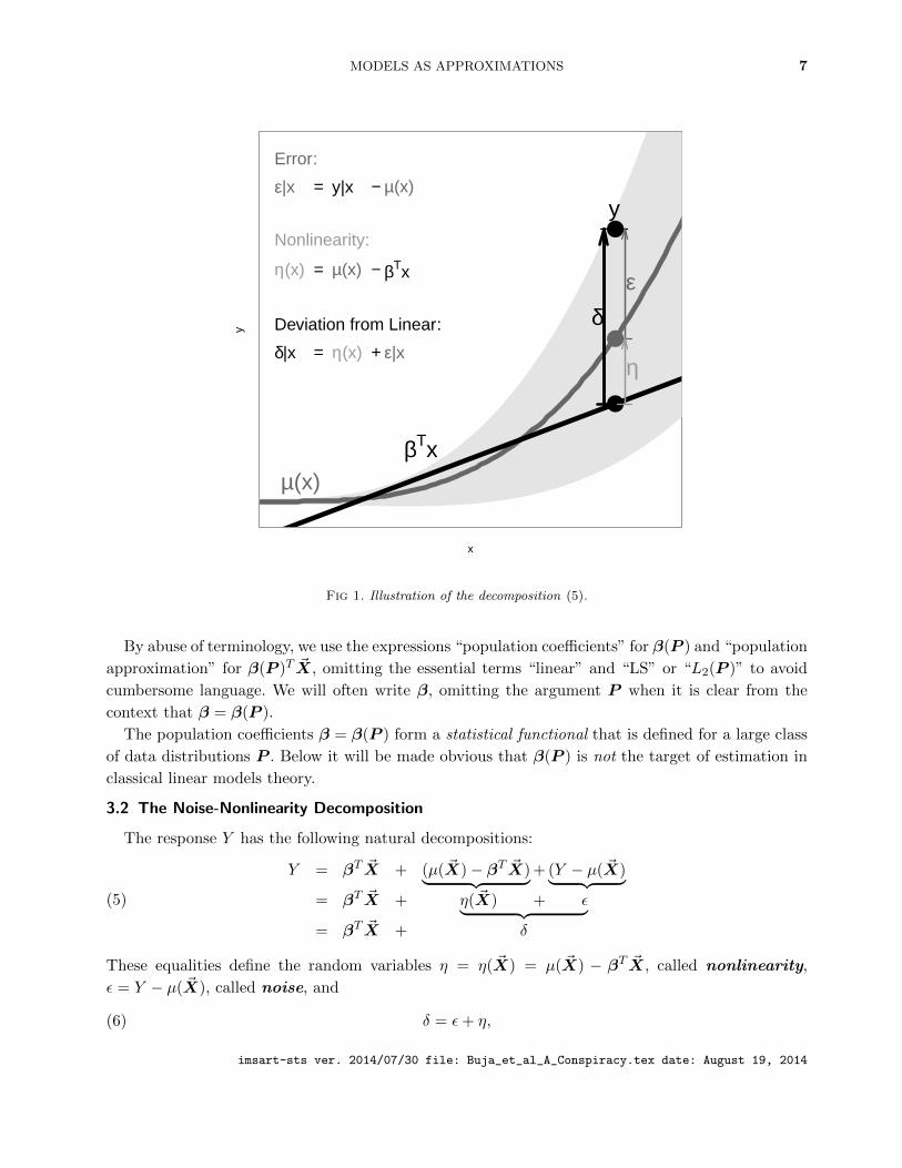
Error:
ε|x = y|x − µ(x)
Nonlinearity:
η(x) = µ(x) − βTx
Deviation from Linear:
δ|x = η(x) + ε|x
Fig 1. Illustration of the decomposition (5).
By abuse of terminology, we use the expressions “population coefficients” for β(P ) and “population
approximation” for β(P )T ~X, omitting the essential terms “linear” and “LS” or “L2(P )” to avoid
cumbersome language. We will often write β, omitting the argument P when it is clear from the
context that β = β(P ).
The population coefficients β = β(P ) form a statistical functional that is defined for a large class
of data distributions P . Below it will be made obvious that β(P ) is not the target of estimation in
classical linear models theory.
3.2 The Noise-Nonlinearity Decomposition
The response Y has the following natural decompositions:
(5)
Y = βT ~X + (µ( ~X)− βT ~X)︸ ︷︷ ︸+ (Y − µ( ~X)︸ ︷︷ ︸= βT ~X + η( ~X) + ε︸ ︷︷ ︸= βT ~X + δ
These equalities define the random variables η = η( ~X) = µ( ~X) − βT ~X, called nonlinearity,
ε = Y − µ( ~X), called noise, and
(6) δ = ε+ η,
imsart-sts ver. 2014/07/30 file: Buja_et_al_A_Conspiracy.tex date: August 19, 2014
8 A. BUJA ET AL.
for which there does not exist a standard term, hence the name “total deviation” (from linearity)
may suffice. An attempt to depict the decompositions (5) for a single predictor is given in Figure 1.
The noise ε is not assumed homoskedastic, and its conditional distributions P (dε| ~X) can be quite
arbitrary except for being centered and having second moments almost surely:
E[ ε | ~X]P= 0,(7)
σ2( ~X) := V [ ε | ~X] = E[ ε2 | ~X]P< ∞.(8)
In addition to the conditional variance σ2( ~X), we will need the conditional mean squared
error m2( ~X) of the population LS linear function, and its variance-bias2 decomposition associated
with (6):
(9) m2( ~X) := E[ δ2 | ~X] = σ2( ~X) + η2( ~X).
3.3 Interpretations and Properties of the Decompositions
Equations (5) above can be given the following semi-parametric interpretation:
(10)µ( ~X)︸ ︷︷ ︸ = βT ~X︸ ︷︷ ︸ + η( ~X)︸ ︷︷ ︸ .
semi-parametric part parametric part nonparametric part
Thus the proposed purpose of linear regression is to extract the parametric part of the response
surface and provide statistical inference for the parameters in the presence of a nonparametric part.
To make the decomposition (10) identifiable one needs an orthogonality constraint:
E[ (βT ~X) η( ~X) ] = 0.
For η( ~X) as defined in (5), this equality follows from the more general fact that the nonlinearity
η( ~X) is orthogonal to all predictors. Because we will need similar facts for ε and δ as well, we state
them all at once:
(11) E[ ~X η ] = 0, E[ ~X ε ] = 0, E[ ~X δ ] = 0.
Proofs: η ⊥ ~X because it is the population residual of the regression of µ( ~X) on ~X according to
(13) below; ε ⊥ ~X because E[ ~Xε] = E[ ~XE[ε| ~X]] = 0. Finally, δ ⊥ ~X i because δ = η + ε.
As a consequence of the inclusion of an intercept in ~X, centering follows as a special case of (11):
(12) E[ε] = E[η] = E[δ] = 0.
3.4 Error Terms in Econometrics
In econometric models, where predictors are treated as random, there exists a need to specify
how error terms relate stochastically to the predictors. While statisticians would assume errors to
be independent of predictors, there is a tendency in econometrics to assume orthogonality only:
E[ error · ~X] = 0. This weaker condition, however, inadvertently permits nonlinearities as part
of the “error” because nonlinearities η are indeed uncorrelated with the predictors according to
(11), though not independent from them. Thus econometricians’ error terms appear to be the total
imsart-sts ver. 2014/07/30 file: Buja_et_al_A_Conspiracy.tex date: August 19, 2014
MODELS AS APPROXIMATIONS 9
deviations δ = ε+ η. The unusual property of δ as “error term” is that generally E[ δ | ~X] 6= 0 in the
assumption-lean framework, even though E[ δ ] = 0 holds always.
The implications may not always be clear, as the following two examples show: Hausman (1978),
in an otherwise groundbreaking article, seems to imply that E[ error · ~X] = 0 is equivalent to
E[ error | ~X] = 0 (ibid., p.1251, (1.1a)), which it isn’t. White’s (1980b, p.818) famous article on
heteroskedasticity-consistent standard errors also uses the weaker orthogonality assumption, but
he is clear that his misspecification test addresses both nonlinearity and heteroskedasticity (ibid.,
p.823). He is less clear about the fact that “heteroskedasticity-consistent” standard errors are also
“nonlinearity-consistent”, even though this is spelled out clearly in his lesser-known article on “Using
Least Squares to Approximate Unknown Regression Functions” (White 1980a, p.162-3). For this
reason the latter article is the more relevant one for us even though it uses an idiosyncratic framework.
As nonlinearity is the more consequential model deviation than heteroskedasticity, the synonym
“heteroskedasticity-consistent estimator” for the sandwich estimator is somewhat misleading.
What statisticians are more likely to recognize as “error” is ε as defined above; yet they will have
misgiving as well because ε is the deviation not from the fitted approximate model but from the true
response surface. We therefore call it “noise” rather than “error.” The noise ε is not independent
of the predictors either, but because E[ε| ~X] = 0 it enjoys a stronger orthogonality property than
the nonlinearity η: E[ g( ~X) ε ] = 0 for all g( ~X) ∈ L2(P ). For full independence one would need the
property E[ g( ~X)h(ε) ] = 0 for all centered g( ~X), h(ε) ∈ L2(P ), which is not generally the case.
Facts:
• The error ε is independent of ~X iff the conditional distribution of ε given ~X is the same across
predictor space: E[f(ε) | ~X]P= E[f(ε)] ∀f(ε) ∈ L2 (which implies heteroskedasticity).
• The nonlinearity η is independent of ~X iff it vanishes: ηP= 0.
• The total deviation δ is independent of ~X iff both the error ε is independent of ~X and ηP= 0.
As technically trivial as these facts are, they show that stochastic independence of errors and pre-
dictors is a strong assumption that rules out both nonlinearities and heteroskedasticities. (This form
of independence is to be distinguished from the assumption of i.i.d. errors in the linear model where
the predictors are fixed.) A hint of unclarity in this regard can be detected even in White (1980b,
p.824, footnote 5) when he writes “specification tests ... may detect only a lack of independence
between errors and regressors, instead of misspecification.” However, “lack of independence” is mis-
specification, which is to first order nonlinearity and to second order heteroskedasticity. What White
apparently had in mind are higher order violations of independence. Note that misspecification in the
weak sense of violation of orthogonality of errors and predictors is not a meaningful concept: neither
nonlinearities nor heteroskedastic noise would qualify as misspecifications as both are orthogonal to
the predictors by construction (see Sections 3.2 and 3.3).
4. NON-ANCILLARITY OF THE PREDICTOR DISTRIBUTION
We show in detail that the principle of predictor ancillarity does not hold when models are ap-
proximations rather than generative truths. For some background on ancillarity, see Appendix A.
It is clear that the population coefficients β(P ) do not depend on all details of the joint (Y, ~X)
distribution. For one thing, they are blind to the noise ε. This follows from the fact that β(P ) is also
imsart-sts ver. 2014/07/30 file: Buja_et_al_A_Conspiracy.tex date: August 19, 2014

10 A. BUJA ET AL.
X
Y
Y = µ(X)
X
Y
Y = µ(X)
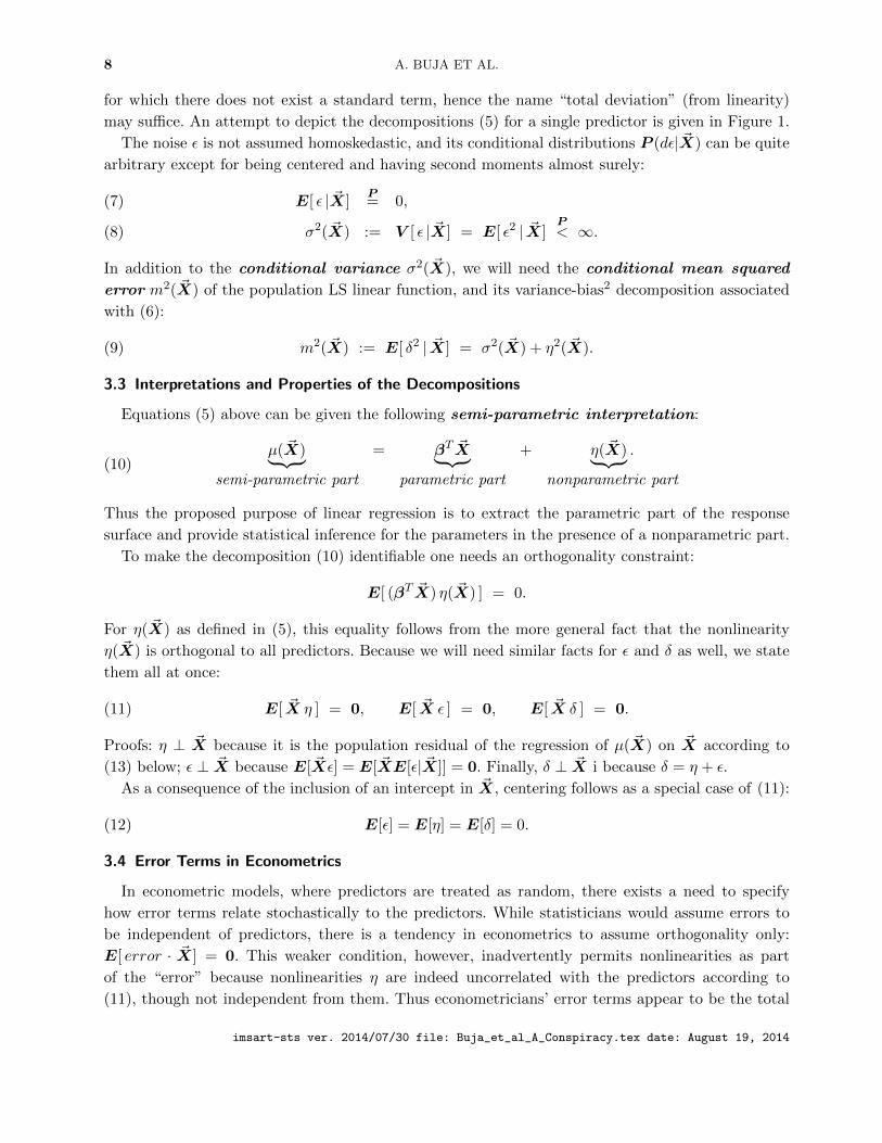
Fig 2. Illustration of the dependence of the population LS solution on the marginal distribution of the predictors: Theleft figure shows dependence in the presence of nonlinearity; the right figure shows independence in the presence oflinearity.
the best linear L2(P ) approximation to µ( ~X):
(13) β(P ) = argminβ∈IRp+1 E[(µ( ~X)− βT ~X)2] = E[ ~X ~XT
]−1E[ ~Xµ( ~X) ] .
This may be worth spelling out in detail:
Lemma: The LS functional β(P ) depends on P only through the conditional mean function and the
predictor distribution; it does not depend on the conditional noise distribution. That is, for two data
distributions P 1(dy,d~x) and P 2(dy,d~x) the following holds:
P 1(d~x) = P 2(d~x), µ1( ~X)P 1,2= µ2( ~X) =⇒ β(P 1) = β(P 2).
The next and most critical question is whether β(P ) depends on the predictor distribution at all.
If the ancillarity argument for predictors is to be believed, the distribution of the predictors should
be unrelated to β(P ). The facts, however, are as follows:
Proposition: The LS functional β(P ) does not depend on the predictor distribution if and only
if µ( ~X) is linear. More precisely, for a fixed measurable function µ0(~x) consider the class of data
distributions P for which µ0(.) is a version of their conditional mean function: E[Y | ~X] = µ( ~X)P=
µo( ~X). In this class the following holds:
µ0(.) is nonlinear =⇒ ∃P 1,P 2 : β(P 1) 6= β(P 2),
µ0(.) is linear =⇒ ∀P 1,P 2 : β(P 1) = β(P 2).
imsart-sts ver. 2014/07/30 file: Buja_et_al_A_Conspiracy.tex date: August 19, 2014
MODELS AS APPROXIMATIONS 11
X
Y Y = µ(X)
P2(dx)
P1(dx)
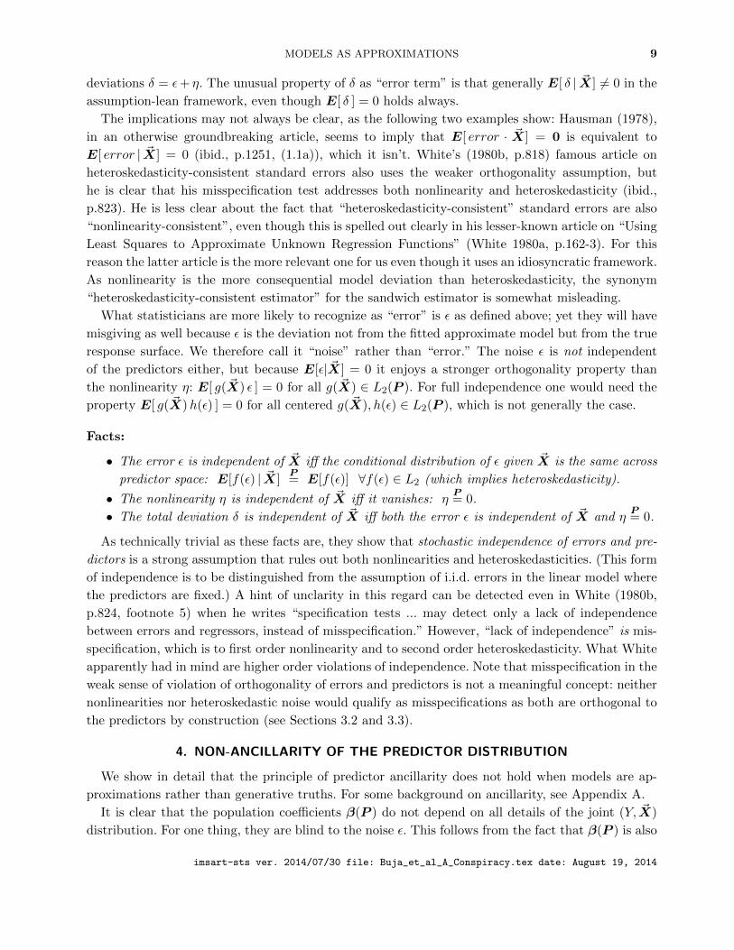
Fig 3. Illustration of the interplay between predictors’ high-density range and nonlinearity: Over the small range of P 1
the nonlinearity will be undetectable and immaterial for realistic sample sizes, whereas over the extended range of P 2
the nonlinearity is more likely to be detectable and relevant.
(For the simple proof details, see Appendix B.2.) In the nonlinear case the clause ∃P 1,P 2 :
β(P 1) 6= β(P 2) is driven solely by differences in the predictor distributions P 1(d~x) and P 2(d~x)
because P 1 and P 2 share the mean function µ0(.) while their conditional noise distributions are
irrelevant by the above lemma.
The proposition is much more easily explained with a graphical illustration: Figure 2 shows single
predictor situations with a nonlinear and a linear mean function, respectively, and the same two
predictor distributions. The two population LS lines for the two predictor distributions differ in the
nonlinear case and they are identical in the linear case. (This observation appears first in White
(1980a, p.155-6); to see the correspondence, identify Y with his g(Z) + ε.)
The relevance of the proposition is that in the presence of nonlinearity the LS functional β(P )
depends on the predictor distribution, hence the predictors are not ancillary for β(P ). The concept
of ancillarity in generative models has things upside down in that it postulates independence of
the predictor distribution from the parameters of interest. In a semi-parametric framework where
the fitted function is an approximation and the parameters are statistical functionals, the matter
presents itself in reverse: It is not the parameters that affect the predictor distribution; rather, it is
the predictor distribution that affects the parameters.
imsart-sts ver. 2014/07/30 file: Buja_et_al_A_Conspiracy.tex date: August 19, 2014
12 A. BUJA ET AL.
The loss of predictor ancillarity has practical implications: Consider two empirical studies that use
the same predictor and response variables. If their statistical inferences about β(P ) seem superficially
contradictory, there may yet be no contradiction if the response surface is nonlinear and the predictor
distributions in the two studies differ: it is then possible that the two studies differ in their targets
of estimation, β(P 1) 6= β(P 2). A difference in predictor distributions in two studies implies in
general a difference in the best fitting linear approximation, as illustrated by Figure 2. Differences
in predictor distributions can become increasingly complex and harder to detect as the predictor
dimension increases.
If at this point one is tempted to recoil from the idea of models as approximations and revert
to the idea that models must be well-specified, one should expect little comfort: The very idea of
well-specification is a function of the high-density range of predictor distributions because over a
small range a model has a better chance of appearing “well-specified” for the simple reason that
approximations work better over small ranges . This is illustrated by Figure 3: the narrow range of
the predictor distribution P 1(d~x) is the reason why the linear approximation is excellent, that is,
the model is very nearly “well specified”, whereas the wide range of P 2(d~x) is the reason for the
gross “misspecification” of the linear approximation. This is a general issue that cannot be resolved
by calls for more “substantive theory” in modeling: Even the best of theories have limited ranges of
validity as has been shown by the most successful theories known to science, those of physics.
5. OBSERVATIONAL DATASETS, ESTIMATION, AND CLTS
Turning to estimation from i.i.d. data, it will be shown how the variability in the LS estimate can
be asymptotically decomposed into two sources: nonlinearity and noise.
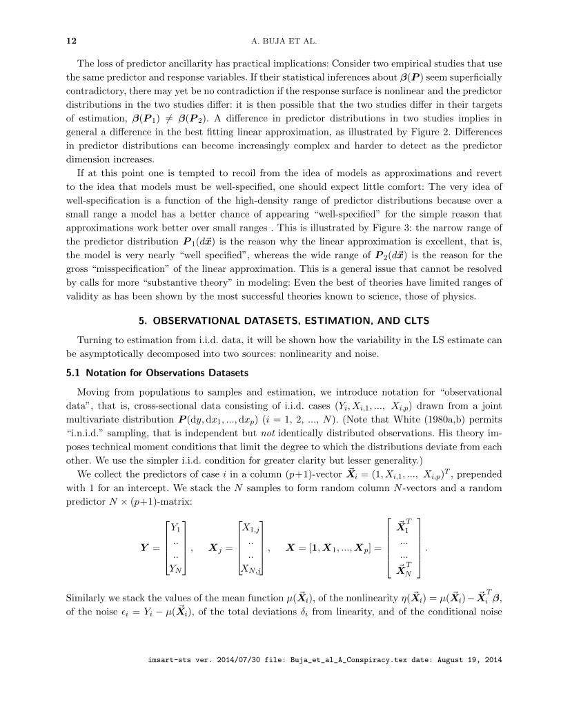
5.1 Notation for Observations Datasets
Moving from populations to samples and estimation, we introduce notation for “observational
data”, that is, cross-sectional data consisting of i.i.d. cases (Yi, Xi,1, ..., Xi,p) drawn from a joint
multivariate distribution P (dy,dx1, ...,dxp) (i = 1, 2, ..., N). (Note that White (1980a,b) permits
“i.n.i.d.” sampling, that is independent but not identically distributed observations. His theory im-
poses technical moment conditions that limit the degree to which the distributions deviate from each
other. We use the simpler i.i.d. condition for greater clarity but lesser generality.)
We collect the predictors of case i in a column (p+1)-vector ~Xi = (1, Xi,1, ..., Xi,p)T , prepended
with 1 for an intercept. We stack the N samples to form random column N -vectors and a random
predictor N × (p+1)-matrix:
Y =
Y1..
..
YN
, Xj =
X1,j
..
..
XN,j
, X = [1,X1, ...,Xp] =
~XT
1
...
...
~XT
N
.
Similarly we stack the values of the mean function µ( ~Xi), of the nonlinearity η( ~Xi) = µ( ~Xi)− ~XT
i β,
of the noise εi = Yi − µ( ~Xi), of the total deviations δi from linearity, and of the conditional noise
imsart-sts ver. 2014/07/30 file: Buja_et_al_A_Conspiracy.tex date: August 19, 2014
MODELS AS APPROXIMATIONS 13
standard deviations σ( ~Xi) to form random column N -vectors:
(14) µ =
µ( ~X1)
..
..
µ( ~XN )
, η =
η( ~X1)
..
..
η( ~XN )
, ε =
ε1..
..
εN
, δ =
δ1..
..
δN
, σ =
σ( ~X1)
..
..
σ( ~XN )
.The definitions of η( ~X), ε and δ in (5) translate to vectorized forms:
η = µ−Xβ, ε = Y − µ, δ = Y −Xβ.(15)
It is important to keep in mind the distinction between population and sample properties. In partic-
ular, the N -vectors δ, ε and η are not orthogonal to the predictor columns Xj in the sample. Writing
〈·, ·〉 for the usual Euclidean inner product on IRN , we have in general 〈δ,Xj〉 6= 0, 〈ε,Xj〉 6= 0,
〈η,Xj〉 6= 0, even though the associated random variables are orthogonal to Xj in the population:
E[ δXj ] = E[ εXj ] = E[ η( ~X)Xj ] = 0.
The sample linear LS estimate of β is the random column (p+1)-vector
(16) β = (β0, β1, ..., βp)T = argminβ ‖Y −Xβ‖
2 = (XTX)−1XTY .
Randomness of β stems from both the random response Y and the random predictors in X. Asso-
ciated with β are the following:
the hat or projection matrix: H = XT (XTX)−1XT ,
the vector of LS fits: Y = Xβ = HY ,
the vector of residuals: r = Y −Xβ = (I −H)Y .
The vector r of residuals, which arises from β, is distinct from the vector of total deviations δ =
Y −Xβ, which arises from β = β(P ).
5.2 Decomposition of the LS Estimate According to Noise and Nonlinearity
When the predictors are random the sampling variation of the LS estimate β can be additively
decomposed into two components: one due to noise ε and another due to nonlinearity η interacting
with randomness of the predictors. This decomposition is a direct reflection of δ = ε+ η.
In the classical linear models theory, which conditions on X, the target of estimation is E[β|X].
When X is treated as random, the target of estimation is the population LS solution β = β(P ).
The term E[β|X] is then a random vector that is naturally placed between β and β:
(17) β − β = (β −E[β|X]) + (E[β|X]− β)
This decomposition corresponds to the decomposition δ = ε+ η as the following lemma shows.
Definition and Lemma: We define “Estimation Offsets” or “EOs” for short as follows:
(18)
Total EO : β − β = (XTX)−1XTδ,
Error EO : β −E[ β|X] = (XTX)−1XT ε,
Nonlinearity EO : E[ β|X]− β = (XTX)−1XTη.
imsart-sts ver. 2014/07/30 file: Buja_et_al_A_Conspiracy.tex date: August 19, 2014
14 A. BUJA ET AL.
x
y
●●
●●
●
● ●●
●●
xy
●
●
●●
●
●
●●
●●
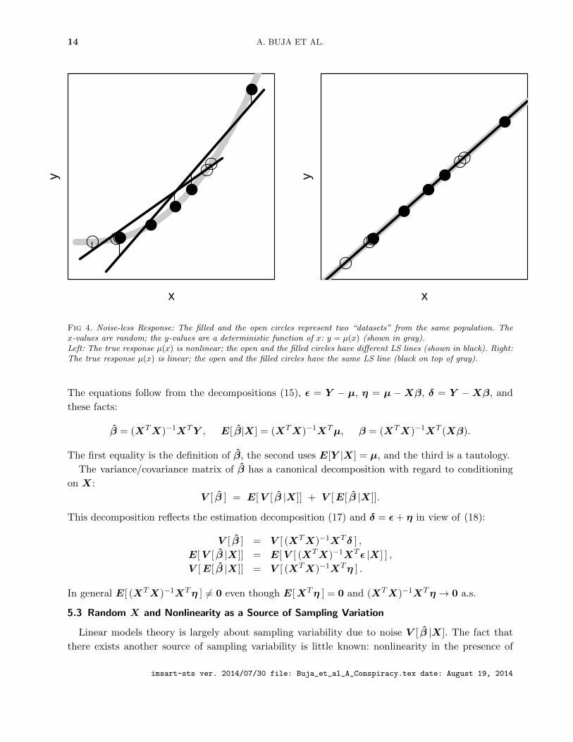
Fig 4. Noise-less Response: The filled and the open circles represent two “datasets” from the same population. Thex-values are random; the y-values are a deterministic function of x: y = µ(x) (shown in gray).Left: The true response µ(x) is nonlinear; the open and the filled circles have different LS lines (shown in black). Right:The true response µ(x) is linear; the open and the filled circles have the same LS line (black on top of gray).
The equations follow from the decompositions (15), ε = Y − µ, η = µ −Xβ, δ = Y −Xβ, and
these facts:
β = (XTX)−1XTY , E[ β|X] = (XTX)−1XTµ, β = (XTX)−1XT (Xβ).
The first equality is the definition of β, the second uses E[Y |X] = µ, and the third is a tautology.
The variance/covariance matrix of β has a canonical decomposition with regard to conditioning
on X:
V [ β ] = E[V [ β |X]] + V [E[ β |X]].
This decomposition reflects the estimation decomposition (17) and δ = ε+ η in view of (18):
V [ β ] = V [ (XTX)−1XTδ ] ,
E[V [ β |X]] = E[V [ (XTX)−1XT ε |X] ] ,
V [E[ β |X]] = V [ (XTX)−1XTη ] .
In general E[ (XTX)−1XTη ] 6= 0 even though E[XTη ] = 0 and (XTX)−1XTη → 0 a.s.
5.3 Random X and Nonlinearity as a Source of Sampling Variation
Linear models theory is largely about sampling variability due to noise V [ β |X]. The fact that
there exists another source of sampling variability is little known: nonlinearity in the presence of
imsart-sts ver. 2014/07/30 file: Buja_et_al_A_Conspiracy.tex date: August 19, 2014
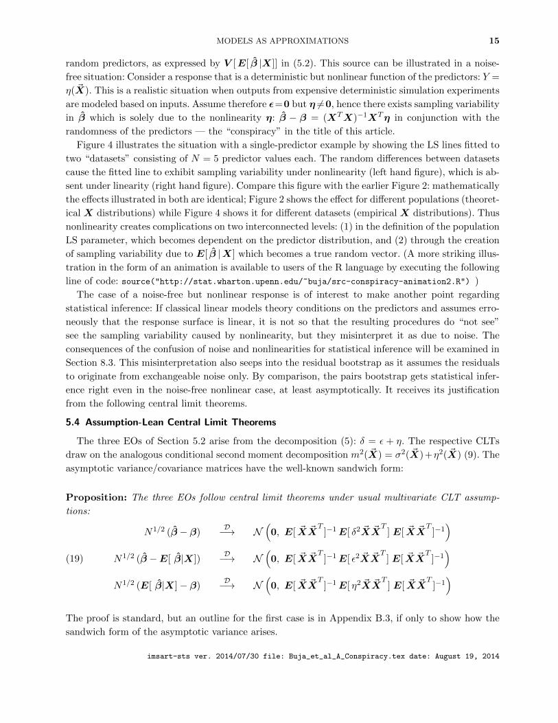
MODELS AS APPROXIMATIONS 15
random predictors, as expressed by V [E[ β |X]] in (5.2). This source can be illustrated in a noise-
free situation: Consider a response that is a deterministic but nonlinear function of the predictors: Y =
η( ~X). This is a realistic situation when outputs from expensive deterministic simulation experiments
are modeled based on inputs. Assume therefore ε=0 but η 6=0, hence there exists sampling variability
in β which is solely due to the nonlinearity η: β − β = (XTX)−1XTη in conjunction with the
randomness of the predictors — the “conspiracy” in the title of this article.
Figure 4 illustrates the situation with a single-predictor example by showing the LS lines fitted to
two “datasets” consisting of N = 5 predictor values each. The random differences between datasets
cause the fitted line to exhibit sampling variability under nonlinearity (left hand figure), which is ab-
sent under linearity (right hand figure). Compare this figure with the earlier Figure 2: mathematically
the effects illustrated in both are identical; Figure 2 shows the effect for different populations (theoret-
ical X distributions) while Figure 4 shows it for different datasets (empirical X distributions). Thus
nonlinearity creates complications on two interconnected levels: (1) in the definition of the population
LS parameter, which becomes dependent on the predictor distribution, and (2) through the creation
of sampling variability due to E[ β |X] which becomes a true random vector. (A more striking illus-
tration in the form of an animation is available to users of the R language by executing the following
line of code: source("http://stat.wharton.upenn.edu/~buja/src-conspiracy-animation2.R") )
The case of a noise-free but nonlinear response is of interest to make another point regarding
statistical inference: If classical linear models theory conditions on the predictors and assumes erro-
neously that the response surface is linear, it is not so that the resulting procedures do “not see”
see the sampling variability caused by nonlinearity, but they misinterpret it as due to noise. The
consequences of the confusion of noise and nonlinearities for statistical inference will be examined in
Section 8.3. This misinterpretation also seeps into the residual bootstrap as it assumes the residuals
to originate from exchangeable noise only. By comparison, the pairs bootstrap gets statistical infer-
ence right even in the noise-free nonlinear case, at least asymptotically. It receives its justification
from the following central limit theorems.
5.4 Assumption-Lean Central Limit Theorems
The three EOs of Section 5.2 arise from the decomposition (5): δ = ε + η. The respective CLTs
draw on the analogous conditional second moment decomposition m2( ~X) = σ2( ~X)+η2( ~X) (9). The
asymptotic variance/covariance matrices have the well-known sandwich form:
Proposition: The three EOs follow central limit theorems under usual multivariate CLT assump-
tions:
(19)
N1/2 (β − β)D−→ N
(0, E[ ~X ~X
T]−1E[ δ2 ~X ~X
T] E[ ~X ~X
T]−1)
N1/2 (β −E[ β|X])D−→ N
(0, E[ ~X ~X
T]−1E[ ε2 ~X ~X
T] E[ ~X ~X
T]−1)
N1/2 (E[ β|X]− β)D−→ N
(0, E[ ~X ~X
T]−1E[ η2 ~X ~X
T] E[ ~X ~X
T]−1)
The proof is standard, but an outline for the first case is in Appendix B.3, if only to show how the
sandwich form of the asymptotic variance arises.
imsart-sts ver. 2014/07/30 file: Buja_et_al_A_Conspiracy.tex date: August 19, 2014
16 A. BUJA ET AL.
The center parts of the first two asymptotic sandwich covariances can equivalently be written as
(20) E[m2( ~X) ~X ~XT
] = E[ δ2 ~X ~XT
], E[σ2( ~X) ~X ~XT
] = E[ ε2 ~X ~XT
],
which follows from m2( ~X) = E[ δ2| ~X] and σ2( ~X) = E[ ε2| ~X] according to (8) and (9).
The proposition can be specialized in a few ways to cases of partial or complete well-specification:
• First order well-specification: When there is no nonlinearity, η( ~X)P= 0, then
N1/2 (β − β)D−→ N
(0, E[ ~X ~X
T]−1E[ ε2 ~X ~X
T] E[ ~X ~X
T]−1)
The sandwich form of the asymptotic variance/covariance matrix is solely due to heteroskedas-
ticity.
• First and second order well-specification: When additionally homoskedasticity holds,
σ2( ~X)P= σ2, then
N1/2 (β − β)D−→ N
(0, σ2E[ ~X ~X
T]−1)
The familiar simplified form is asymptotically valid under first and second order well-specification
but without the assumption of Gaussian noise.
• Deterministic nonlinear response: When σ2( ~X)P= 0, then
N1/2 (β − β)D−→ N
(0, E[ ~X ~X
T]−1E[ η2 ~X ~X
T] E[ ~X ~X
T]−1)
The sandwich form of the asymptotic variance/covariance matrix is solely due to nonlinearity
and random predictors.
6. THE SANDWICH ESTIMATOR AND THE M -OF-N PAIRS BOOTSTRAP
Empirically one observes that standard error estimates obtained from the pairs bootstrap and
from the sandwich estimator are generally close to each other. This is intuitively unsurprising as
they both estimate the same asymptotic variance, that of the first CLT in (30). A closer connection
between them will be established below.
6.1 The Plug-In Sandwich Estimator of Asymptotic Variance
According to (19) the asymptotic variance of the LS estimator β is
(21) AV [β] = E[ ~X ~XT
]−1E[ δ2 ~X ~XT
] E[ ~X ~XT
]−1.
The sandwich estimator is then the plug-in version of (21) where δ2 is replaced by residuals and
population expectations E[...] by sample means E[...]:
E[ ~X ~XT
] = 1N
∑i=1...N
~Xi~XT
i = 1N (XTX)
E[ r2 ~X ~XT
] = 1N
∑i=1...N r
2i~Xi~XT
i = 1N (XTD2
rX),
where D2r is the diagonal matrix with squared residuals r2i = (Yi− ~Xiβ)2 in the diagonal. With this
notation the simplest and original form of the sandwich estimator of asymptotic variance can be
imsart-sts ver. 2014/07/30 file: Buja_et_al_A_Conspiracy.tex date: August 19, 2014
MODELS AS APPROXIMATIONS 17
written as follows (White 1980a):
(22)AVsand := E[ ~X ~X
T]−1 E[ r2 ~X ~X
T] E[ ~X ~X
T]−1
= N (XTX)−1 (XTD2rX) (XTX)−1
The sandwich standard error estimate for the j’th regression coefficient is therefore obtained as
(23) SEsand[βj ] := 1N1/2 (AVsand)
1/2jj .
For this simplest version (“HC” in MacKinnon and White (1985)) obvious modifications exist. For one
thing, it does not account for the fact that residuals have on average smaller variance than noise. An
overall correction factor (N/(N −p−1))1/2 in (23) would seem to be sensible in analogy to the linear
models estimator ( “HC1” ibid.). More detailed modifications have been proposed whereby individual
residuals are corrected for their reduced conditional variance according to V [ri|X] = σ2(1 − Hii)
under homoskedasticity and ignoring nonlinearity (“HC2” ibid.). Further modifications include a
version based on the jackknife (“HC3” ibid.) using leave-one-out residuals. An obvious alternative is
estimating asymptotic variance with the pairs bootstrap, to which we now turn.
6.2 The M -of-N Pairs Bootstrap Estimator of Asymptotic Variance
To connect the sandwich estimator to its bootstrap counterpart we need the M -of-N bootstrap
whereby the resample size M is allowed to differ from the sample size N . It is at this point important
not to confuse
• M -of-N resampling with replacement, and
• M -out-of-N subsampling without replacement.
In resampling the resample size M can be any M <∞, whereas for subsampling it is necessary that
the subsample size M satisfy M < N . We are here concerned with bootstrap resampling, and we
will focus on the extreme case M � N , namely, the limit M →∞.
Because resampling is i.i.d. sampling from some distribution, there holds a CLT as the resample
size grows, M → ∞. It is immaterial that in this case the sampled distribution is the empirical
distribution PN of a given dataset {( ~Xi, Yi)}i=1...N , which is frozen of size N as M →∞.
Proposition: For any fixed dataset of size N , there holds a CLT for the M -of-N bootstrap as
M →∞. Denoting by β∗M the LS estimate obtained from a bootstrap resample of size M , we have
(24) M1/2 (β∗M − β)D−→ N
(0, E[ ~X ~X
T]−1 E[ (Y − ~XT
β)2 ~X ~XT
] E[ ~X ~XT
]−1)
(M →∞).
This is a straight application of the CLT of the previous section to the empirical distribution rather
than the actual distribution of the data, where the middle part (the “meat”) of the asymptotic
formula is based on the empirical counterpart r2i = (Yi− ~XT
i β)2 of δ2 = (Y − ~XTβ)2. A comparison
of (22) and (24) results in the following:
Corollary: The sandwich estimator (22) is the asymptotic variance estimated by the limit of the
M -of-N pairs bootstrap as M →∞ for a fixed sample of size N .
imsart-sts ver. 2014/07/30 file: Buja_et_al_A_Conspiracy.tex date: August 19, 2014
18 A. BUJA ET AL.
As an inferential method the pairs bootstrap is obviously more flexible and richer in possibilities
than the sandwich estimator. The latter is limited to providing a standard error estimate assuming
approximate normality of the parameter estimate’s sampling distribution. The bootstrap distribution,
on the other hand, can be used to generate confidence intervals that are often second order correct
(the literature on this topic is too rich to list, so we point only to the standard bootstrap reference
by Efron and Tibshirani (1994)).
Further connections are mentioned by MacKinnon and White (1985): Some forms of the sandwich
estimator were independently derived by Efron (1982, p.18-19) using the infinitesimal jackknife,
and by Hinkley (1977) using what he calls a “weighted jackknife”. See Weber (1986) for a concise
comparison in the fixed-X linear models framework limited to the problem of heteroskedasticity. A
richer context for the relation between the jackknife and bootstrap is given by Wu (1986)
7. ADJUSTED PREDICTORS
The adjustment formulas of this section serve to express the slopes of multiple regressions as
slopes in simple regressions using adjusted single predictors. The goal is to analyze the discrepancies
between asymptotically proper and improper standard errors of regression estimates, and to provide
tests that indicate for each predictor whether the linear models standard error is invalidated by
“misspecification” (Section 8).
7.1 Adjustment in populations
To express the population LS regression coefficient βj = βj(P ) as a simple regression coefficient,
let the adjusted predictor Xj• be defined as the “residual” of the population regression of Xj , used
as the response, on all other predictors. In detail, collect all other predictors in the random p-vector~X−j = (1, X1, ..., Xj−1, Xj+1, ..., Xp)
T , and let β−j• be the coefficient vector from the regression of Xj
onto ~X−j :
β−j• = argminβ∈IRp E[ (Xj − βT ~X−j)
2] = E[ ~X−j ~XT
−j ]−1E[ ~X−jXj ] .
The adjusted predictor Xj• is the residual from this regression:
(25) Xj• = Xj − ~XT
−jβ−j• .
The representation of βj as a simple regression coefficient is as follows:
(26) βj =E[Y Xj•]
E[Xj•2]
=E[µ( ~X)Xj•]
E[Xj•2]
.
7.2 Adjustment in samples
To express estimates of regression coefficients as simple regressions, we collect all predictor columns
other than Xj in a N × p random predictor matrix X−j = (1, ...,Xj−1,Xj+1, ...) and define
β−j• = argminβ∈IRp ‖Xj −X−jβ‖2 = (XT−jX−j)
−1XT−jXj .
Using the hat notation “•” to denote sample-based adjustment to distinguish it from population-
based adjustment “•”, we write the sample-adjusted predictor as
(27) Xj• = Xj −X−j β−j• = (I −H−j)Xj .
imsart-sts ver. 2014/07/30 file: Buja_et_al_A_Conspiracy.tex date: August 19, 2014
MODELS AS APPROXIMATIONS 19
where H−j = X−j(XT−jX−j)
−1XT−j is the associated projection or hat matrix. The j’th slope estimate
of the multiple linear regression of Y on X1, ...,Xp can then be expressed in the well-known manner
as the slope estimate of the simple linear regression without intercept of Y on Xj•:
(28) βj =〈Y ,Xj•〉‖Xj•‖2
.
In the proofs (see the Appendix) we also need notation for each observation’s population-adjusted
predictors: Xj• = (X1,j•, ..., XN,j•)T = Xj −X−jβ−j•. The following distinction is elementary but
important: The component variables of Xj• = (Xi,j•)i=1...N are i.i.d. as they are population-adjusted,
whereas the component variables of Xj• = (Xi,j•)i=1...N are dependent as they are sample-adjusted.
As N → ∞ for fixed p, this dependency disappears asymptotically, and we have for the empirical
distribution of the values {Xi,j•}i=1...N the obvious convergence in distribution:
{Xi,j•}i=1...ND−→ Xj•
D= Xi,j• (N →∞).
7.3 Adjustment for Estimation Offsets and Their CLTs
The vectorized formulas for estimation offsets (17) can be written componentwise using adjustment
as follows:
(29)
Total EO : βj − βj =〈Xj•, δ〉‖Xj•‖2
,
Error EO : βj −E[ βj |X] =〈Xj•, ε〉‖Xj•‖2
,
Nonlinearity EO : E[ βj |X]− βj =〈Xj•,η〉‖Xj•‖2
.
To see these identities directly, note the following, in addition to (28): E[βj |X] = E[〈µ,Xj•〉]/‖Xj•‖2
and βj = 〈Xβ,Xj•〉/‖Xj•‖2, the latter due to 〈Xj•,Xk〉 = δjk‖Xj•‖2. Finally use δ = Y −Xβ,
η = µ−Xβ and ε = Y −µ.
Asymptotic normality can also be expressed for each βj separately using population adjustment:
Corollary:
(30)
N1/2(βj − βj)D−→ N
(0,E[m2( ~X)Xj•
2]
E[Xj•2]2
)= N
(0,E[ δ2Xj•
2]
E[Xj•2]2
)
N1/2(βj −E[ βj |X])D−→ N
(0,E[σ2( ~X)Xj•
2]
E[Xj•2]2
)= N
(0,E[ ε2Xj•
2]
E[Xj•2]2
)
N1/2(E[ βj |X]− βj)D−→ N
(0,E[ η2( ~X)Xj•
2]
E[Xj•2]2
)These are not new results but reformulations for the components of the vector CLTs (19). The
equalities in the first and second case are based on (20). The asymptotic variances of (30) are the
subject of next section.
imsart-sts ver. 2014/07/30 file: Buja_et_al_A_Conspiracy.tex date: August 19, 2014
20 A. BUJA ET AL.
8. ASYMPTOTIC VARIANCES — PROPER AND IMPROPER
The following prepares the ground for an asymptotic comparison of linear models standard errors
with correct assumption-lean standard errors. We know the former to be potentially incorrect in the
presence of nonlinearity and/or heteroskedasticity, hence a natural question is: by how much can
linear models standard errors deviate from valid assumption-lean standard errors? We look for an
answer in the asymptotic limit, which frees us from issues related to how the standard errors are
estimated.
8.1 Proper Asymptotic Variances in Terms of Adjusted Predictors
The CLTs (30) contain three asymptotic variances, one for the estimate βj and two for the contri-
butions due to noise and due to nonlinearity according to m2( ~X) = σ2( ~X)+η( ~X). These asymptotic
variances are of the same functional form, which suggests using generic notation for all three. We
therefore define:
Definition:
(31) AV(j)lean[f2( ~X)] :=
E[ f2( ~X)Xj•2]
E[Xj•2]2
Using m2( ~X) = σ2( ~X)+η2( ~X) from (9), we obtain a decomposition of asymptotic variance suggested
by (30):
(32)
AV(j)lean[m2( ~X)] = AV
(j)lean[σ2( ~X) + AV
(j)lean[η2( ~X)]
E[m2( ~X)Xj•2]
E[Xj•2]2
=E[σ2( ~X)Xj•
2]
E[Xj•2]2
+E[ η2( ~X)Xj•
2]
E[Xj•2]2
8.2 Improper Asymptotic Variances in Terms of Adjusted Predictors
Next we write down an asymptotic form for the conventional standard error estimate from linear
models theory in the assumption-lean framework. This asymptotic form will have the appearance of
an asymptotic variance but it will generally be improper as its intended domain of validity is the
assumption-loaded framework of linear models theory. This “improper” asymptotic variance derives
from an estimate σ2 of the noise variance, usually σ2 = ‖Y −Xβ‖2/(N−p−1). In the assumption-lean
framework with both heteroskedastic error variance and nonlinearity, σ2 has the following limit for
fixed p:
σ2P−→ E[m2( ~X) ] = E[σ2( ~X) ] +E[ η2( ~X) ], N →∞.
Squared standard error estimates for coefficients are, in matrix form and adjustment form, as follows:
(33) V lin[ β ] = σ2 (XTX)−1, SE2lin[ βj ] =
σ2
‖Xj•‖2.
Their scaled limits under lean assumptions are as follows:
(34) N V lin[ β ]P−→ E[m2( ~X) ] E[ ~X ~X
T]−1, N SE
2lin[ βj ]
P−→ E[m2( ~X) ]
E[X2j• ]
.
imsart-sts ver. 2014/07/30 file: Buja_et_al_A_Conspiracy.tex date: August 19, 2014
MODELS AS APPROXIMATIONS 21
We call these limits “improper asymptotic variances”. Again we can use (9) m2( ~X) = σ2( ~X) +
η2( ~X) for a decomposition and therefore introduce generic notation where f2( ~X) is a placeholder
for any one among m2( ~X), σ2( ~X) and η2( ~X):
Definition:
(35) AV(j)lin [f2( ~X)] :=
E[ f2( ~X)]
E[Xj•2]
Hence this the improper asymptotic variance of βj and its decomposition:
(36)
AV(j)lin [m2( ~X)] = AV
(j)lin [σ2( ~X)] + AV
(j)lin [η2( ~X)]
E[m2( ~X)]
E[Xj•2]
=E[σ2( ~X)]
E[Xj•2]
+E[ η2( ~X)]
E[Xj•2]
8.3 Comparison of Proper and Improper Asymptotic Variances: RAV
We examine next the discrepancies between proper and improper asymptotic variances by forming
their ratio. It will be shown that this ratio can be arbitrarily close to 0 and to ∞. It can be formed
separately for each of the versions corresponding to m2( ~X), σ2( ~X) and η2( ~X). For this reason we
introduce a generic form of the ratio:
Definition: Ratio of Asymptotic Variances, Proper/Improper.
(37) RAVj [f2( ~X)] :=
AV(j)lean[f2( ~X)]
AV(j)lin [f2( ~X)]
=E[f2( ~X)Xj•
2]
E[f2( ~X)]E[Xj•2]
Again, f2( ~X) is a placeholder for each of m2( ~X), σ2( ~X) and η2( ~X). The overall RAVj [m2( ~X)] can
be decomposed into a weighted average of RAVj [σ2( ~X)] and RAVj [η
2( ~X)]:
Lemma: RAV Decomposition.
(38)
RAVj [m2( ~X)] = wσRAVj [σ
2( ~X)] + wηRAVj [η2( ~X)]
wσ :=E[σ2( ~X)]
E[m2( ~X)], wη :=
E[η2( ~X)]
E[m2( ~X)], wσ + wη = 1.
Implications of this decomposition will be discussed below. Structurally, the three ratios RAVj can
be interpreted as inner products between the normalized squared random variables
m2( ~X)
E[m2( ~X)],
σ2( ~X)
E[σ2( ~X)],
η2( ~X)
E[η2( ~X)]
imsart-sts ver. 2014/07/30 file: Buja_et_al_A_Conspiracy.tex date: August 19, 2014
22 A. BUJA ET AL.
on the one hand, and the normalized squared adjusted predictor
Xj•2
E[Xj•2]
on the other hand. These inner products, however, are not correlations, and they are not bounded
by +1; their natural bounds are rather 0 and ∞, both of which can generally be approached to any
degree as will be shown in Subsection 8.5.
8.4 The Meaning of RAV
The ratio RAVj [m2( ~X)] shows by what multiple the proper asymptotic variance deviates from the
improper one:
• If RAVj [m2( ~X)] = 1, then SElin[βj ] is asymptotically correct;
• if RAVj [m2( ~X)] > 1, then SElin[βj ] is asymptotically too small/optimistic;
• if RAVj [m2( ~X)] < 1, then SElin[βj ] is asymptotically too large/pessimistic.
If, for example, RAVj [m2( ~X)] = 4, then, for large sample sizes, the proper standard error of
βj is about twice as large as the improper standard error of linear models theory. If, however,
RAVj [m2( ~X)] = 1, it does not imply that the model is well-specified because heteroskedasticity and
nonlinearity can conspire to makeRAVj [m2( ~X)] = 1 even though neither σ2(X) = const nor η( ~X) =
0; see the decomposition lemma in Subsection 8.3. If, for example, m2( ~X) = σ2( ~X) + η2( ~X) = m20
constant while neither σ2( ~X) is constant nor η2( ~X) vanishes, then RAVj [m20] = 1 and the linear
models standard error is asymptotically correct, yet the model is “misspecified.” Well-specification
to first and second order, η( ~X) = 0 and σ2( ~X) = σ20 constant, is a sufficient but not necessary
condition for asymptotic validity of the conventional standard error.
8.5 The Range of RAV
As mentioned RAV ratios can generally vary between 0 and ∞. The following proposition states
the technical conditions under which these bounds are sharp. The formulation is generic in terms of
f2( ~X) as placeholder for m2( ~X), σ2( ~X) and η2( ~X). The proof is in Appendix B.4.
Proposition:
(a) If Xj• has unbounded support on at least one side, that is, if P [Xj•2 > t] > 0 ∀t > 0, then
(39) supfRAVj [f
2( ~X)] =∞ .
(b) If the closure of the support of the distribution of Xj• contains zero (its mean) but there is no
pointmass at zero, that is, if P [Xj•2 < t] > 0 ∀t > 0 but P [Xj•
2 = 0] = 0, then
(40) inffRAVj [f
2( ~X)] = 0 .
As a consequence, it is in general the case that RAVj [m2( ~X)], RAVj [σ
2( ~X)] and RAVj [η2( ~X)] can
each range between 0 and ∞. (A slight subtlety arises from the constraint imposed on η( ~X) by
orthogonality (11) to the predictors, but it does not invalidate the general fact.)
imsart-sts ver. 2014/07/30 file: Buja_et_al_A_Conspiracy.tex date: August 19, 2014
MODELS AS APPROXIMATIONS 23
The proposition involves only some plausible conditions on the distribution of Xj•, not all of ~X.
This follows from the fact that the dependence of RAVj [f2( ~X)] on the distribution of ~X can be
reduced to dependence on the distribution of Xj•2 through conditioning:
(41) RAVj [f2( ~X)] =
E[f2j (Xj•)Xj•2]
E[f2j (Xj•]E[Xj•2]
where f2j (Xj•) := E[f2( ~X) |Xj•2].
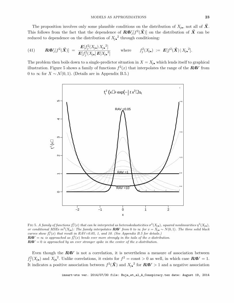
The problem then boils down to a single-predictor situation in X = Xj• which lends itself to graphical
illustration. Figure 5 shows a family of functions f2(x) that interpolates the range of the RAV from
0 to ∞ for X ∼ N (0, 1). (Details are in Appendix B.5.)
−2 −1 0 1 2
01
23
45
x
f t 2 (x
)
t
−0.90
−0.50
−0.25
0.00
0.50
1 2 4 8 19RAV =10
RAV =0.05
RAV =1
ft 2 (x) = exp(− 1
2 t x2) st
Fig 5. A family of functions f2t (x) that can be interpreted as heteroskedasticities σ2(Xj•), squared nonlinearities η2(Xj•),
or conditional MSEs m2(Xj•): The family interpolates RAV from 0 to ∞ for x = Xj• ∼ N(0, 1). The three solid blackcurves show f2
t (x) that result in RAV=0.05, 1, and 10. (See Appendix B.5 for details.)RAV =∞ is approached as f2
t (x) bends ever more strongly in the tails of the x-distribution.RAV = 0 is approached by an ever stronger spike in the center of the x-distribution.
Even though the RAV is not a correlation, it is nevertheless a measure of association between
f2j (Xj•) and Xj•2. Unlike correlations, it exists for f2 = const > 0 as well, in which case RAV = 1.
It indicates a positive association between f2( ~X) and Xj•2 for RAV > 1 and a negative association
imsart-sts ver. 2014/07/30 file: Buja_et_al_A_Conspiracy.tex date: August 19, 2014
24 A. BUJA ET AL.
●
●
●●●
●
●
●
●
●
●
●●
●●
●
●
●
●
●
●●
●
●
●
●●
●
●
● ●
●●
●
●
●
●
●
●●
●
●
●
●
●
●
●
●
●
●
●
●
●
● ●●
●
●
●
●●
●
●
●
●●
●
●●
●
●●
●
●●
●
●
●
●
●
●
●●●
●
●
●
●
●
●
●●
●
●
●
●
●
●
●
●
●●●
●
●
●
●
●
●
● ● ●●
●
●●
●
●
●●
●●
●
●
●
●
●
●
●●
●
●
●
●
●●●
●
●
●●
●
●
●
●●
●
●●
●
●
●
●
●
●
●
●●●
●
●
●
●
●
●
●
●
●
●
●
● ●
●
●
●
●
●●
●
●
●● ●●
●
●
●
●
●
●
●
●
●
●
●
●
●●
●
●
●
●
●
●
●
●
●●
●●
●
●
●
●
●
●●
●
●
●
●
●
●
●●
● ●●
●
●
●
●
●
●
●
●
●
●
●
●● ●
●●
●
●
●
●
●
●
●
●
●
●
●
●
●
●
●
●
●●
●●
●
●
●
●
●
●
●
●
●
●
●
●
●
●
●
●
●
●
●●
●
●
●
●
●
●●
●
●
●
●
●
●
●
●●
●
●
●
●
●
●
●
●
●
●
●
●
●
●
●
●
● ●
●
●
●
●
●
●
●
●
●
●
●
●
●
●
●
●
●
●
●
●
●
●
●
●
●●
●
●
●
●●
●
●
●
●●
● ●
●●
●
●
●
●● ●
●
●●
●
●
●
●●
●
●
●
● ●
●
●
●
●
●
●●
●
●
●●
●●
●
●
●
●
●●● ●
●
● ●
●
●
●
●
●
● ●
●
●●● ●●
●
●●
●
●
●
●
●
●
●
●
●
●
●
●
● ●
●
●
●
●
●
●
●
●
●●
●● ●
●
●
●
●
●
● ●
●
●
●
●
●
●
●●
●
●
●●
●
●●
●
●●
●
●
● ●
●●
●
● ●
●
●
●
●
●
●
●● ●
●
●
●
● ●
●
●
●
●
● ●
●●
−1.0 −0.5 0.0 0.5 1.0
−4
−2
02
4
x
yRAV ~ 2
●
●
●
●
●
●● ●●
●
●
●
●
●
●●
●
●
●
●
●
●
●
●
●
●●
●●
● ●
●
●
●
●
●
●
●
●
●
●
●
●
●● ●
●
●
●
●
●
●
●
●
●●
●
●
●
●●
●
●
●●●
●
●
●
●
● ●
●●
●●
●
●
●
●
●
●
●
●
●
●
●
● ●
●
● ●
●
●
●
●
●
●●
●
●
●
●
●
●●●●●●
●
●
●●
●
●
●
●
●
●●
●●
●
●
●
●
●
●
●
●
●●
●
●● ●
●● ●●
●●
●
●●
●●●
●
●
●
●●
●
●
●
●
●
●
●
●
●
●
●
●
●
●
●
●
●
●
●
●
●
●●
●
● ●●
●●
●●
●
●●
●
●●
●
●
●
●
●●
●
●
●
●
●●
●
●●
●
●
●
●
●●
●
●●●
●
●
●
●●
●
●
●
●
●
●●
●
●
●
●
●●
●
●
●
●●
●
●
●
●
●
●
●●
●●
●
●●
●
●●
●
●
●●
●●
●
●
●
●●
●
●
● ●
●
●●
●
●
●
●
●
●
●
●
●
●
●
● ●
●
●
●
●●
●
●
●
●
●●
●
●
●
●●
●
●●
●
●●●
●●
●
●
●
●
●
●
●
●
●●
●
●
●
●
●●
● ●
●
●●
●
●
●●
●
●
●
●
●
●
●
●
●
●
●
●
●
●
●●
●
●
●
●●
●
●
●
●●
●
●
●
●
●
●
●●
●●●
● ●●
●
●
●●
●
●
●
●
●
●
●
●
●
●
●
●
●
●
●
●
●
●
●
●
●
●●
● ●
●
●
●
●
●
●
●
●
●
●●
●●
● ●●
●●
●●
●
●
●
●
●●
●●
●
●
●
●● ●●
●
●●
●
●
●
●
●
●
● ●●
●
●
●
●●
●
●
●
●
●
●
●●
●●
●
●
●
●
●
●
● ●
●
●
●
●
●
●
●
●
●
●
●
●
●
●●● ●●
●
●●
●
●
●
●
−1.0 −0.5 0.0 0.5 1.0
−4
−2
02
4
x
y
RAV ~ 0.08
●
●
●
●
●
●
●
●
●
●
●
●
●
●
●
●
●
●
●
●●
●
●
●
●
●
●
●
●
●
●
●
●
●
●
●
●
●
●●●
●
●
●●
●
●
●
●
●
●
●●
●
●●
●
●
●
●
●
●
●
●
●
● ●
●
●
●
●
●
●
●
●
●
●
●
●
●
●
●
●
●
●
●
●
●
●
●
●
●
●
●
●
●
●
●
●
●
●
●
●
●●
●
●
●●
●
● ●
●
●
●
●
●
●
●
●●
●
●
●
●●
●
●
●
●
●
●●
●
●
●
●
●
●● ●
●
●
●
●
●
●
●
●
●
●
●
●
●
●
●●
●
●●
●●
●
●
●
●
●
●● ●●
●
●
●
●
●
●
●
●
●
●●
●
●●
●
●
●●
●
●
●
●
●
●
●
●
●
●
●
●
●
●
●●
●
●
●
●
● ●
●
●
●●
●
●
●
●
●
●
● ●
●
●
●
●
●
●
●
●
●●
●
●
●
● ●
●
●
●
●
●
●
●
●●
●
●
●
●●
●
●●
●●
●
●
●●
●
●
●
●
●
●
●
●
●
●
●
●
●
●
●
●● ●
●
●
●
●●
●
●
●
●
●
●
●
●
●
●
●●
●
●
●
●
●
●
●
●●
●
●
●
●
●●
●●
●
●
●● ●
●
●
●
●●●
●
●
●
●
●
●
●
●●
●
●
●
●
●●
●●
●
●
●
● ●
●
●
●
●
●
●
●
●
●
●
●
●●
●
●
●
●
●
●
●
●
●
●
●●
●
●
●
●
●
●
●
●
●
●
●
●
●
●
●
●
●
●
●
●
● ●
●
●
●
●
●●
●
●
●●
●
●
●
●
●
●
●
●
●
●
●
●
●
●
●
●
●●
●
●
●
●
●
●
●
●
●
●
●●
●●
●
●
●●
●
●
●
● ●
●
●
●
●
●
●
●
● ●
● ●
●
●
●
●
●
● ●
●●●
●
●
●
●●
●
●
●
●
●
●●
●
●
●
●
●
●
●
●
●
●●
●
●●
●●●
●
●
●
●
●
●
−1.0 −0.5 0.0 0.5 1.0
−4
−2
02
4
x
y
RAV ~ 1
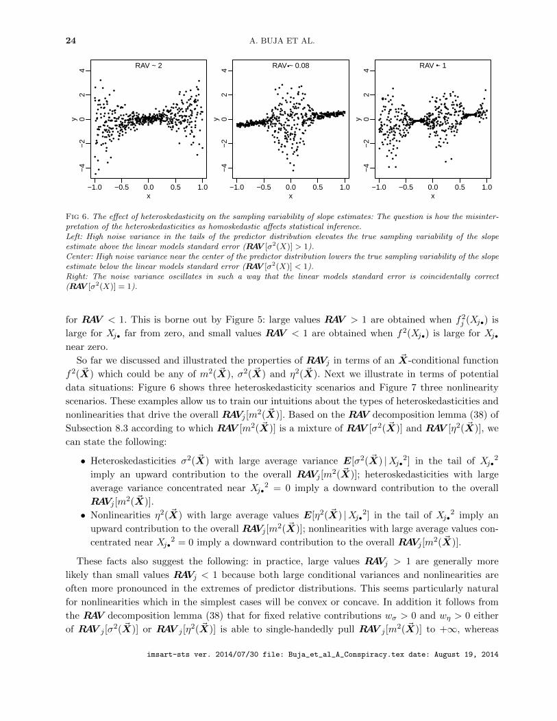
Fig 6. The effect of heteroskedasticity on the sampling variability of slope estimates: The question is how the misinter-pretation of the heteroskedasticities as homoskedastic affects statistical inference.Left: High noise variance in the tails of the predictor distribution elevates the true sampling variability of the slopeestimate above the linear models standard error (RAV [σ2(X)] > 1).Center: High noise variance near the center of the predictor distribution lowers the true sampling variability of the slopeestimate below the linear models standard error (RAV [σ2(X)] < 1).Right: The noise variance oscillates in such a way that the linear models standard error is coincidentally correct(RAV [σ2(X)] = 1).
for RAV < 1. This is borne out by Figure 5: large values RAV > 1 are obtained when f2j (Xj•) is
large for Xj• far from zero, and small values RAV < 1 are obtained when f2(Xj•) is large for Xj•near zero.
So far we discussed and illustrated the properties of RAVj in terms of an ~X-conditional function
f2( ~X) which could be any of m2( ~X), σ2( ~X) and η2( ~X). Next we illustrate in terms of potential
data situations: Figure 6 shows three heteroskedasticity scenarios and Figure 7 three nonlinearity
scenarios. These examples allow us to train our intuitions about the types of heteroskedasticities and
nonlinearities that drive the overall RAVj [m2( ~X)]. Based on the RAV decomposition lemma (38) of
Subsection 8.3 according to which RAV [m2( ~X)] is a mixture of RAV [σ2( ~X)] and RAV [η2( ~X)], we
can state the following:
• Heteroskedasticities σ2( ~X) with large average variance E[σ2( ~X) |Xj•2] in the tail of Xj•2
imply an upward contribution to the overall RAVj [m2( ~X)]; heteroskedasticities with large
average variance concentrated near Xj•2 = 0 imply a downward contribution to the overall
RAVj [m2( ~X)].
• Nonlinearities η2( ~X) with large average values E[η2( ~X) |Xj•2] in the tail of Xj•2 imply an
upward contribution to the overall RAVj [m2( ~X)]; nonlinearities with large average values con-
centrated near Xj•2 = 0 imply a downward contribution to the overall RAVj [m
2( ~X)].
These facts also suggest the following: in practice, large values RAVj > 1 are generally more
likely than small values RAVj < 1 because both large conditional variances and nonlinearities are
often more pronounced in the extremes of predictor distributions. This seems particularly natural
for nonlinearities which in the simplest cases will be convex or concave. In addition it follows from
the RAV decomposition lemma (38) that for fixed relative contributions wσ > 0 and wη > 0 either
of RAV j [σ2( ~X)] or RAV j [η
2( ~X)] is able to single-handedly pull RAV j [m2( ~X)] to +∞, whereas
imsart-sts ver. 2014/07/30 file: Buja_et_al_A_Conspiracy.tex date: August 19, 2014
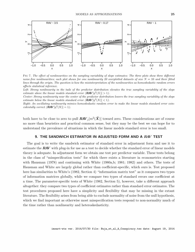
MODELS AS APPROXIMATIONS 25
−1.0 −0.5 0.0 0.5 1.0
−2
02
4
x
y
●
●
●
●
● ●
●
●
●●●● ●
●
●
●
●
●
●
●
● ●
●
●
●
●
●
●●
●
●
●
●
●
●
●
●
●
●
●
●
●
●●
●
●
●
●
●
●
● ●●
●
●
●
●●●
●
RAV ~ 3.5
−1.0 −0.5 0.0 0.5 1.0
−2
02
4
x
y
●
●
●
●
●●
●●
●
●●
●
●
●●
●
●
●
●
●
●●
●
●
●
●
●
●●
●
●
●
●
●
●
●
●
●●
●
●
●
●
●
●
●
●
●
●
●
●
●
●
●
●
●
●
●
●
●
RAV ~ 0.17
−1.0 −0.5 0.0 0.5 1.0
−2
02
4
x
y
●●
●
●
●
●
●
●
●
●●
●
●
●
●
●
●
●
●
●
●
●
●
●
●
●
●
●
●
●
●
●
●
●
●
●
●
●
●
●
●
●
●
●
●
●
●
●
●
●
●
●
●
●
●
●
●
●
●
●
RAV ~ 1
Fig 7. The effect of nonlinearities on the sampling variability of slope estimates: The three plots show three differentnoise-free nonlinearities; each plot shows for one nonlinearity 20 overplotted datasets of size N = 10 and their fittedlines through the origin. The question is how the misinterpretation of the nonlinearities as homoskedastic random errorsaffects statistical inference.Left: Strong nonlinearity in the tails of the predictor distribution elevates the true sampling variability of the slopeestimate above the linear models standard error (RAV [η2(X)] > 1).Center: Strong nonlinearity near the center of the predictor distribution lowers the true sampling variability of the slopeestimate below the linear models standard error (RAV [η2(X)] < 1).Right: An oscillating nonlinearity mimics homoskedastic random error to make the linear models standard error coin-cidentally correct (RAV [η2(X)] = 1).
both have to be close to zero to pull RAV j [m2( ~X)] toward zero. These considerations are of course
no more than heuristics and practical common sense, but they may be the best we can hope for to
understand the prevalence of situations in which the linear models standard error is too small.
9. THE SANDWICH ESTIMATOR IN ADJUSTED FORM AND A RAV TEST
The goal is to write the sandwich estimator of standard error in adjustment form and use it to
estimate the RAV with plug-in for use as a test to decide whether the standard error of linear models
theory is adequate. In adjustment form we obtain one test per predictor variable. These tests belong
in the class of “misspecification tests” for which there exists a literature in econometrics starting
with Hausman (1978) and continuing with White (1980a,b; 1981; 1982) and others. The tests of
Hausman and White are largely global rather than coefficient-specific, which ours is. Test proposed
here has similarities to White’s (1982, Section 4) “information matrix test” as it compares two types
of information matrices globally, while we compare two types of standard errors one coefficient at
a time. The parameter-specific tests of White (1982, Section 5), however, take a different approach
altogether: they compare two types of coefficient estimates rather than standard error estimates. The
test procedures proposed here have a simplicity and flexibility that may be missing in the extant
literature. The flexibility arises from being able to exclude normality of noise from the null hypothesis,
which we find important as otherwise most misspecification tests respond to non-normality much of
the time rather than nonlinearity and heteroskedasticity.
imsart-sts ver. 2014/07/30 file: Buja_et_al_A_Conspiracy.tex date: August 19, 2014
26 A. BUJA ET AL.
9.1 The Adjustment Form of the Sandwich Estimator and the ˆRAVj Statistic
To begin with, the adjustment versions of the asymptotic variances in the CLTs (30) can be used
to rewrite the sandwich estimator by replacing expectations E[...] with means E[...], the population
parameter β with its estimate β, and population adjustment Xj• with sample adjustment Xj•:
(42) AV(j)sand =
E[ (Y − ~XTβ)2Xj•
2]
E[Xj•2]2
= N〈(Y −Xβ)2,Xj•
2〉‖Xj•‖4
The squaring of N -vectors is meant to be coordinate-wise. Formula (42) is not a new estimator of
asymptotic variance; rather, it is an algebraically equivalent re-expression of the diagonal elements of
AVsand in (22) above: AV(j)sand = (AVsand)j,j . The sandwich standard error estimate (23) can therefore
be written as follows:
(43) SEsand(βj) =〈(Y −Xβ)2,Xj•
2〉1/2
‖Xj•‖2.
The usual standard error estimate from linear models theory is (33):
(44) SElin(βj) =σ
‖Xj•‖=
‖Y −Xβ‖(N−p−1)1/2 ‖Xj•‖
.
In order to translate RAVj [m2( ~X)] into a practically useful diagnostic, an obvious first attempt
would be forming the ratio SEsand(βj)/SElin(βj), squared. However, SElin(βj) has been corrected
for fitted degrees of freedom, whereas SEsand(βj) has not. For greater comparability one would either
correct the sandwich estimator with a factor (N/(N−p−1))1/2 (MacKinnon and White 1985) or else
“uncorrect” SElin(βj) by replacing N−p−1 with N in the variance estimate σ2. Either way one obtains
the natural plug-in estimate of RAVj :
(45) ˆRAVj := N〈(Y −Xβ)2,Xj•
2〉‖Y −Xβ‖2 ‖Xj•‖2
=E[ (Y − ~X
Tβ)2Xj•
2 ]
E[ (Y − ~XTβ)2 ] E[Xj•
2 ].
This diagnostic quantity can be used as a test statistic, as will be shown next. The functional form
of RAVj(m2( ~X)) and its estimate ˆRAVj illuminates a remark by White (1982) on his “Information
Matrix Test for Misspecification” for general ML estimation: “In the linear regression framework, the
test is sensitive to forms of heteroskedasticity or model misspecification which result in correlations
between the squared regression errors and the second order cross-products of the regressors” (ibid.,
p.12). We know now what function of the predictors actually matters for judging the effects of
misspecification on inference for a particular regression coefficient: it is the squared adjusted predictor
and its association with the squared total deviations as estimated by residuals.
9.2 A ˆRAVj Test
There exist several ways to generate inference based on the ˆRAVj , two of which we discuss in this
section, but only one of which can be recommended in practice. We start with an asymptotic result
that would be expected to yield approximately valid retention intervals under a null hypothesis of
well-specification.
imsart-sts ver. 2014/07/30 file: Buja_et_al_A_Conspiracy.tex date: August 19, 2014
MODELS AS APPROXIMATIONS 27
Proposition: If the total deviations δi are independent of ~Xi (not assuming normality of δi) we
have:
(46) N1/2 ( ˆRAVj − 1)D−→ N
(0,E[ δ4]
E[ δ2]2E[Xj•
4]
E[Xj•2]2− 1)
)If one assumes δi ∼ N (0, σ2), then the asymptotic variance simplifies using E[ δ4]/E[ δ2]2 = 3.
As always we ignore moment conditions among the assumptions. A proof outline is in Appendix B.6.
According to (46) it is the kurtoses (= the standardized fourth moments - 3) of total deviation
δ and of the adjusted predictor Xj• that drive the asymptotic variance of ˆRAVj under the null
hypothesis. We note the following facts:
1. Because standardized fourth moments are always ≥ 1 by Jensen’s inequality, the asymptotic
variance is ≥ 0, as it should be. The minimal standardized fourth moment of +1 is attained
by a two-point distribution symmetric about 0. Thus a zero asymptotic variance of ˆRAVj is
achieved when both the total deviations δi and the adjusted predictor Xi,j• have two-point
distributions.
2. The larger the kurtosis of δ or Xj•, the less likely it is that first and second order model mis-
specification can be detected because the larger the asymptotic standard errors will be. It is an
important fact that elevated kurtosis of δ and Xj• obscures nonlinearity and heteroskedasticity.
Yet, if such misspecification can be detected in spite of elevated kurtoses, it is news worth
knowing.
3. A test of the stronger hypothesis that includes normality of δ is obtained by settingE[δ4]/E[δ2]2
= 3 rather than estimating it. However, the resulting test turns into a non-normality test much
of the time. As non-normality can be diagnosed separately with normality tests or normal
quantile plots of the residuals, we recommend keeping normality out of the null hypothesis and
test independence of δ and Xj• alone.
The asymptotic result of the proposition provides insights, but unfortunately it is in our experience
not suitable for practical application. The standard procedure would be to estimate the asymptotic
null variance of ˆRAVj , rescale to sample size N , and use it to form a retention interval around the
null value RAVj = 1. The problem is that the null distribution of ˆRAVj in finite datasets can be non-
normal in such a way that is not easily overcome by obvious tools such as logarithmic transformations.
Not all is lost, however, because non-asymptotic simulation-based approaches to inference exist
for the type of null hypothesis in question. Because the null hypothesis is independence between the
total deviation δ and the adjusted predictor Xj•, a permutation test offers itself. To this end it is
necessary that N � p, and the test will not be exact. The reason is that one needs to estimate the
total deviations δi with residuals ri and the population adjusted predictor values Xi,j• with sample
adjusted predictor values Xi,j•. This test is for the weak hypothesis that does not include normality
of δi and therefore permits general (centered) noise distributions. A retention interval should be
formed directly from the α/2 and 1−α/2 quantiles of the permutation distribution. Quantile-based
intervals can be asymmetric according to the skewness and other idiosyncrasies of the permutation
distribution. Computations inside the permutation simulation are cheap: Once standardized squared
vectors r2/‖r‖2 and Xj•/‖Xj•‖2 are formed, a draw from the conditional null distribution of ˆRAVj
imsart-sts ver. 2014/07/30 file: Buja_et_al_A_Conspiracy.tex date: August 19, 2014
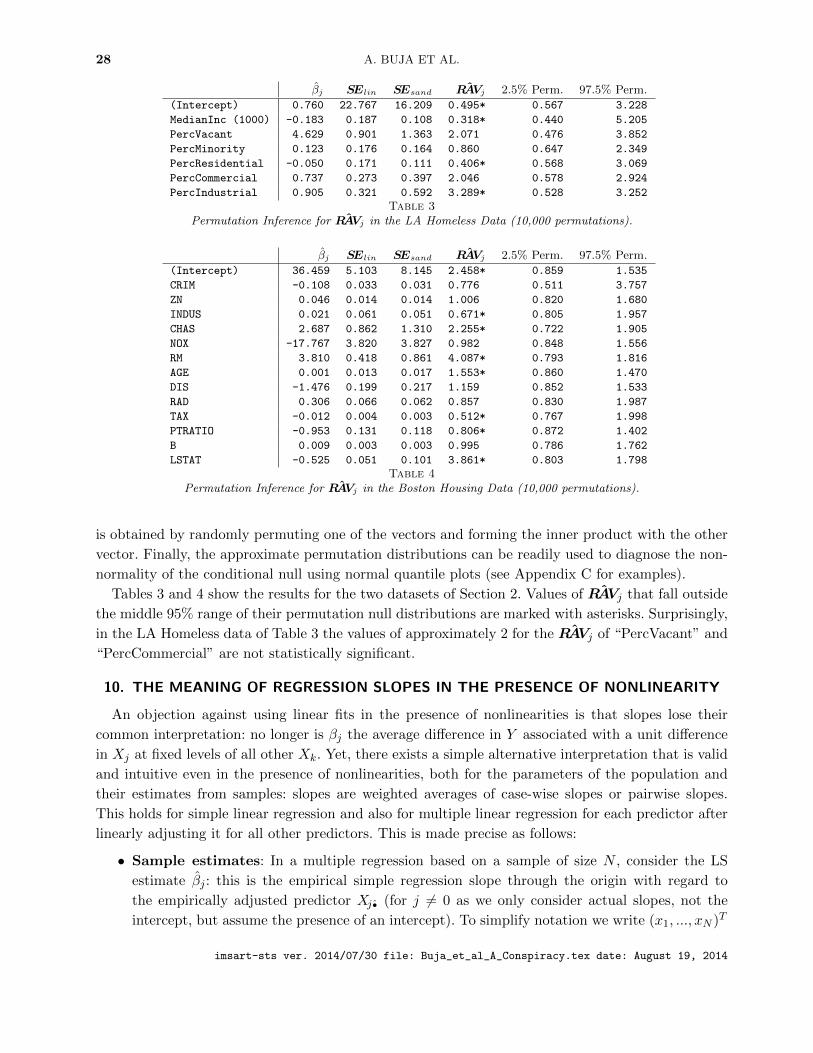
28 A. BUJA ET AL.
βj SElin SEsandˆRAVj 2.5% Perm. 97.5% Perm.
(Intercept) 0.760 22.767 16.209 0.495* 0.567 3.228
MedianInc (1000) -0.183 0.187 0.108 0.318* 0.440 5.205
PercVacant 4.629 0.901 1.363 2.071 0.476 3.852
PercMinority 0.123 0.176 0.164 0.860 0.647 2.349
PercResidential -0.050 0.171 0.111 0.406* 0.568 3.069
PercCommercial 0.737 0.273 0.397 2.046 0.578 2.924
PercIndustrial 0.905 0.321 0.592 3.289* 0.528 3.252Table 3
Permutation Inference for ˆRAVj in the LA Homeless Data (10,000 permutations).
βj SElin SEsandˆRAVj 2.5% Perm. 97.5% Perm.
(Intercept) 36.459 5.103 8.145 2.458* 0.859 1.535
CRIM -0.108 0.033 0.031 0.776 0.511 3.757
ZN 0.046 0.014 0.014 1.006 0.820 1.680
INDUS 0.021 0.061 0.051 0.671* 0.805 1.957
CHAS 2.687 0.862 1.310 2.255* 0.722 1.905
NOX -17.767 3.820 3.827 0.982 0.848 1.556
RM 3.810 0.418 0.861 4.087* 0.793 1.816
AGE 0.001 0.013 0.017 1.553* 0.860 1.470
DIS -1.476 0.199 0.217 1.159 0.852 1.533
RAD 0.306 0.066 0.062 0.857 0.830 1.987
TAX -0.012 0.004 0.003 0.512* 0.767 1.998
PTRATIO -0.953 0.131 0.118 0.806* 0.872 1.402
B 0.009 0.003 0.003 0.995 0.786 1.762
LSTAT -0.525 0.051 0.101 3.861* 0.803 1.798Table 4
Permutation Inference for ˆRAVj in the Boston Housing Data (10,000 permutations).
is obtained by randomly permuting one of the vectors and forming the inner product with the other
vector. Finally, the approximate permutation distributions can be readily used to diagnose the non-
normality of the conditional null using normal quantile plots (see Appendix C for examples).
Tables 3 and 4 show the results for the two datasets of Section 2. Values of ˆRAVj that fall outside
the middle 95% range of their permutation null distributions are marked with asterisks. Surprisingly,
in the LA Homeless data of Table 3 the values of approximately 2 for the ˆRAVj of “PercVacant” and
“PercCommercial” are not statistically significant.
10. THE MEANING OF REGRESSION SLOPES IN THE PRESENCE OF NONLINEARITY
An objection against using linear fits in the presence of nonlinearities is that slopes lose their
common interpretation: no longer is βj the average difference in Y associated with a unit difference
in Xj at fixed levels of all other Xk. Yet, there exists a simple alternative interpretation that is valid
and intuitive even in the presence of nonlinearities, both for the parameters of the population and
their estimates from samples: slopes are weighted averages of case-wise slopes or pairwise slopes.
This holds for simple linear regression and also for multiple linear regression for each predictor after
linearly adjusting it for all other predictors. This is made precise as follows:
• Sample estimates: In a multiple regression based on a sample of size N , consider the LS
estimate βj : this is the empirical simple regression slope through the origin with regard to
the empirically adjusted predictor Xj• (for j 6= 0 as we only consider actual slopes, not the
intercept, but assume the presence of an intercept). To simplify notation we write (x1, ..., xN )T
imsart-sts ver. 2014/07/30 file: Buja_et_al_A_Conspiracy.tex date: August 19, 2014
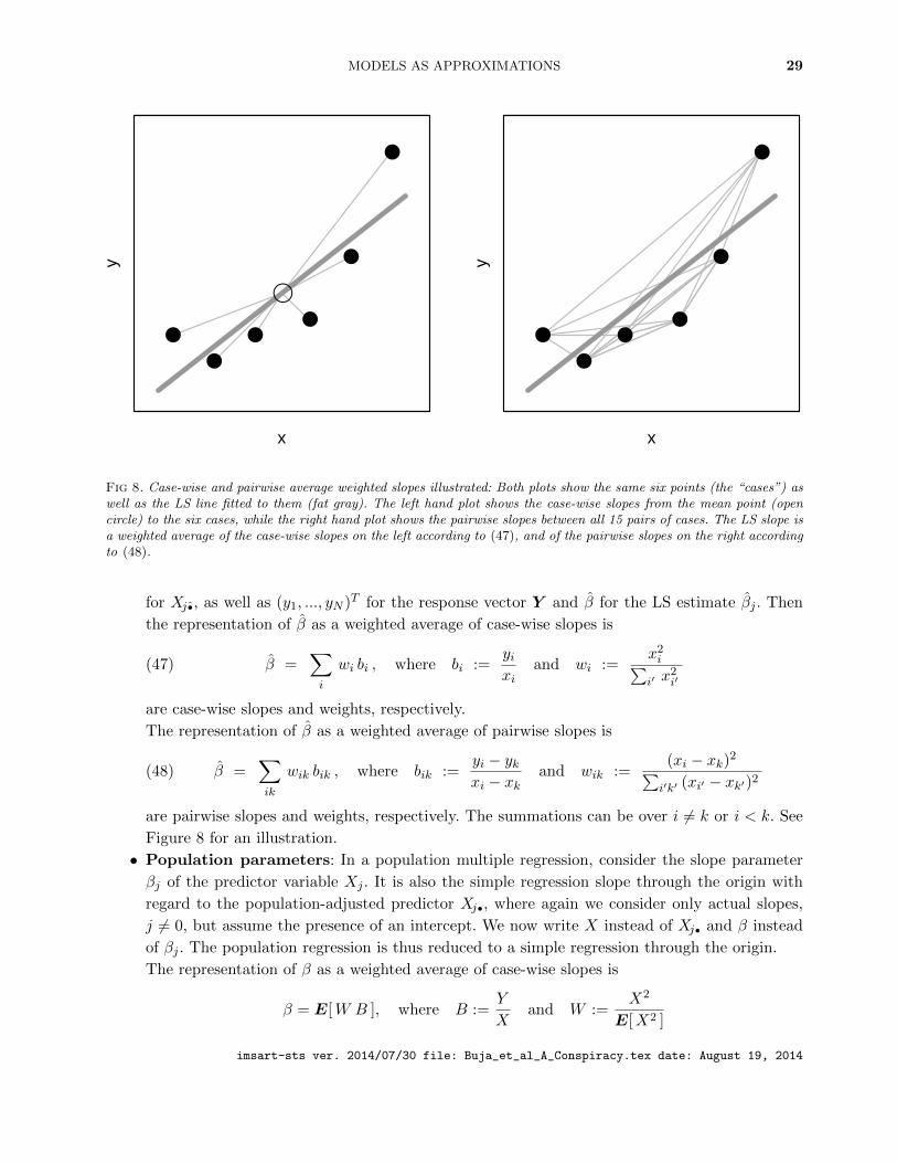
MODELS AS APPROXIMATIONS 29
●
●
●
●
●
●
x
y
●
●
●●
●
●
●
●
●
●
●
●
●
x
y
●
●
●●
●
●
Fig 8. Case-wise and pairwise average weighted slopes illustrated: Both plots show the same six points (the “cases”) aswell as the LS line fitted to them (fat gray). The left hand plot shows the case-wise slopes from the mean point (opencircle) to the six cases, while the right hand plot shows the pairwise slopes between all 15 pairs of cases. The LS slope isa weighted average of the case-wise slopes on the left according to (47), and of the pairwise slopes on the right accordingto (48).
for Xj•, as well as (y1, ..., yN )T for the response vector Y and β for the LS estimate βj . Then
the representation of β as a weighted average of case-wise slopes is
(47) β =∑i
wi bi , where bi :=yixi
and wi :=x2i∑i′ x
2i′
are case-wise slopes and weights, respectively.
The representation of β as a weighted average of pairwise slopes is
(48) β =∑ik
wik bik , where bik :=yi − ykxi − xk
and wik :=(xi − xk)2∑i′k′ (xi′ − xk′)2
are pairwise slopes and weights, respectively. The summations can be over i 6= k or i < k. See
Figure 8 for an illustration.
• Population parameters: In a population multiple regression, consider the slope parameter
βj of the predictor variable Xj . It is also the simple regression slope through the origin with
regard to the population-adjusted predictor Xj•, where again we consider only actual slopes,
j 6= 0, but assume the presence of an intercept. We now write X instead of Xj• and β instead
of βj . The population regression is thus reduced to a simple regression through the origin.
The representation of β as a weighted average of case-wise slopes is
β = E[W B ], where B :=Y
Xand W :=
X2
E[X2 ]
imsart-sts ver. 2014/07/30 file: Buja_et_al_A_Conspiracy.tex date: August 19, 2014
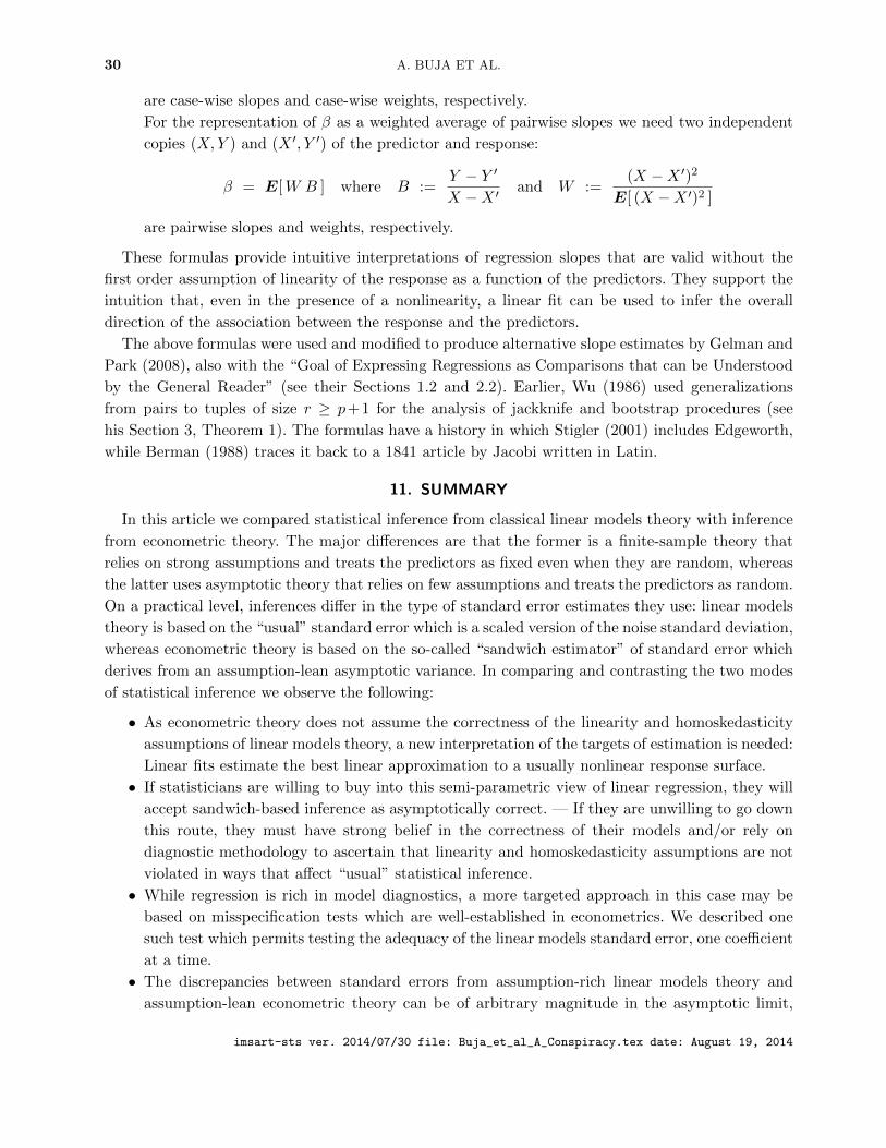
30 A. BUJA ET AL.
are case-wise slopes and case-wise weights, respectively.
For the representation of β as a weighted average of pairwise slopes we need two independent
copies (X,Y ) and (X ′, Y ′) of the predictor and response:
β = E[W B ] where B :=Y − Y ′
X −X ′and W :=
(X −X ′)2
E[ (X −X ′)2 ]
are pairwise slopes and weights, respectively.
These formulas provide intuitive interpretations of regression slopes that are valid without the
first order assumption of linearity of the response as a function of the predictors. They support the
intuition that, even in the presence of a nonlinearity, a linear fit can be used to infer the overall
direction of the association between the response and the predictors.
The above formulas were used and modified to produce alternative slope estimates by Gelman and
Park (2008), also with the “Goal of Expressing Regressions as Comparisons that can be Understood
by the General Reader” (see their Sections 1.2 and 2.2). Earlier, Wu (1986) used generalizations
from pairs to tuples of size r ≥ p+1 for the analysis of jackknife and bootstrap procedures (see
his Section 3, Theorem 1). The formulas have a history in which Stigler (2001) includes Edgeworth,
while Berman (1988) traces it back to a 1841 article by Jacobi written in Latin.
11. SUMMARY
In this article we compared statistical inference from classical linear models theory with inference
from econometric theory. The major differences are that the former is a finite-sample theory that
relies on strong assumptions and treats the predictors as fixed even when they are random, whereas
the latter uses asymptotic theory that relies on few assumptions and treats the predictors as random.
On a practical level, inferences differ in the type of standard error estimates they use: linear models
theory is based on the “usual” standard error which is a scaled version of the noise standard deviation,
whereas econometric theory is based on the so-called “sandwich estimator” of standard error which
derives from an assumption-lean asymptotic variance. In comparing and contrasting the two modes
of statistical inference we observe the following:
• As econometric theory does not assume the correctness of the linearity and homoskedasticity
assumptions of linear models theory, a new interpretation of the targets of estimation is needed:
Linear fits estimate the best linear approximation to a usually nonlinear response surface.
• If statisticians are willing to buy into this semi-parametric view of linear regression, they will
accept sandwich-based inference as asymptotically correct. — If they are unwilling to go down
this route, they must have strong belief in the correctness of their models and/or rely on
diagnostic methodology to ascertain that linearity and homoskedasticity assumptions are not
violated in ways that affect “usual” statistical inference.
• While regression is rich in model diagnostics, a more targeted approach in this case may be
based on misspecification tests which are well-established in econometrics. We described one
such test which permits testing the adequacy of the linear models standard error, one coefficient
at a time.
• The discrepancies between standard errors from assumption-rich linear models theory and
assumption-lean econometric theory can be of arbitrary magnitude in the asymptotic limit,
imsart-sts ver. 2014/07/30 file: Buja_et_al_A_Conspiracy.tex date: August 19, 2014
MODELS AS APPROXIMATIONS 31
but real data examples indicate discrepancies by a factors of 2 to be common. This is obviously
relevant because such factors can change a t-statistic from significant to insignificant and vice
versa.
• The pairs bootstrap is seen to be an alternative to the sandwich estimate of standard error.
The latter is the asymptotic limit in the M -of-N bootstrap as M →∞.
Assumption lean inference is not without its problems. A major issue is its non-robustness: compared
to the standard error from linear models theory the sandwich standard error relies on higher order
moments. The non-robustness is fundamentally a consequence of the LS method, which may suggest
that solutions should be obtained through a revival of robustness theory.
REFERENCES
[1] Aldrich (2005). Fisher and Regression. Statistical Science 20 (4), 4001–417.
[2] Angrist, J. D. and Pischke, J.-S. (2009). Mostly Harmless Econometrics, Princeton: Princeton University Press.
[3] Belsley, D. A.., Kuh, E. and Welsch, R. E. (1980). Regression diagnostics: identifying influential data and
sources of collinearity. Wiley series in probability and mathematical statistics. Hoboken, NJ: John Wiley & Sons,
Inc.
[4] Berk, R. A., Kriegler, B. and Yilvisaker, D. (2008). Counting the Homeless in Los Angeles County. in Prob-
ability and Statistics: Essays in Honor of David A. Freedman, Monograph Series for the Institute of Mathematical
Statistics, D. Nolan and S. Speed (eds.)
[5] Berman, M. (1988). A Theorem of Jacobi and its Generalization. Biometrika 75 (4), 779–783.
[6] Box, G. E. P. (1979). Robustness in the Strategy of Scientific Model Building. in Robustness in Statistics: Proceed-
ings of a Workshop (Launer, R. L., and Wilkinson, G. N., eds.) Amsterdam: Academic Press (Elsevier), 201–236.
[7] Buja, A., Hastie, T. and Tibshirani, R. (1989). Linear Smoothers and Additive Models (with discussions and
rejoinder). The Annals of Statistics, 17 (2), 453–555.
[8] Cox, D. R. and Hinkley, D. V. (1974). Theoretical Statistics, London: Chapman & Hall.
[9] Cox, D.R. (1995). Discussion of Chatfield (1995). Journal of the Royal Statistical Society, Series A 158 (3),
455-456.
[10] Freedman, D. A. (1981). Bootstrapping Regression Models. The Annals of Statistics 9 (6), 1218–1228.
[11] Freedman, D. A. (2006). On the So-Called “Huber Sandwich Estimator” and “Robust Standard Errors.” The
American Statistician 60 (4), 299–302.
[12] Gelman, A. and Park, D.. K. (2008). Splitting a Predictor at the Upper Quarter or Third and the Lower Quarter
or Third, The American Statistician 62 (4), 1–8.
[13] Harrison, X. and Rubinfeld, X. (1978). Hedonic prices and the demand for clean air. Journal of Environmental
Economics and Management 5, 81–102.
[14] Efron, B. (1982). The jackknife, the bootstrap and other resampling plans. Philadelphia, PA: Society for Industrial
and Applied Mathematics (SIAM).
[15] Efron, B. and Tibshirani, R. J. (1994). An Introduction to the Bootstrap, Boca Raton, FL: CRC Press.
[16] Hastie, T. J. and Tibshirani, R. J. (1990). Generalized Additive Models, London: Chapman & Hall/CRC
Monographs on Statistics & Applied Probability.
[17] Hausman, J. A. (1978). Specification Tests in Econometrics. Econometrica 46 (6), 1251-1271.
[18] Hinkley, D. V. (1977). Jackknifing in Unbalanced Situations. Technometrics 19, 285–292.
[19] Huber, P. J. (1967). The behavior of maximum likelihood estimation under nonstandard conditions. Proceed-
ings of the Fifth Berkeley Symposium on Mathematical Statistics and Probability, Vol. 1, Berkeley:
University of California Press, 221–233.
[20] Kauermann, G. and Carroll, R. J. (2001). A note on the efficiency of sandwich covariance matrix estimation,
Journal of the American Statistical Association 96(456), 1387-1396.
imsart-sts ver. 2014/07/30 file: Buja_et_al_A_Conspiracy.tex date: August 19, 2014

32 A. BUJA ET AL.
[21] Mammen, E. (1993). Bootstrap and Wild Bootstrap for High Dimensional Linear Models. The Annals of Statistics
21 (1), 255–285.
[22] MacKinnon, J. and White, H. (1985). Some heteroskedasticity-consistent covariance matrix estimators with
improved finite sample properties. Journal of Econometrics 29, 305–325.
[23] Stigler, S. M. (2001). Ancillary History. In State of the Art in Probability and Statistics: Festschrift for Willem
R. van Zwet (M. DeGunst, C. Klaassen and A. van der Vaart, eds.), 555–567.
[24] Weber, N.C. (1986). The Jackknife and Heteroskedasticity (Consistent Variance Estimation for Regression Mod-
els). Economics Letters 20, 161-163.
[25] White, H. (1980). Using Least Squares to Approximate Unknown Regression Functions. International Economic
Review 21 (1), 149-170.
[26] White, H. (1980). A Heteroskedasticity-Consistent Covariance Matrix Estimator and a Direct Test for Het-
eroskedasticity. Econometrica 48, 817-838.
[27] White, H. (1981). Consequences and Detection of Misspecified Nonlinear Regression Models. Journal of the
American Statistical Association 76 (374), 419-433.
[28] White, H. (1982). Maximum Likelihood Estimation of Misspecified Models. Econometrica 50, 1–25.
[29] Wu, C. F. J. (1986). Jackknife, Bootstrap and Other Resampling Methods in Regression Analysis. The Annals
of Statistics 14 (4), 1261–1295.
imsart-sts ver. 2014/07/30 file: Buja_et_al_A_Conspiracy.tex date: August 19, 2014
MODELS AS APPROXIMATIONS 33
APPENDIX A: ANCILLARITY
The facts as layed out in Section 4 amount to an argument against conditioning on predictors in
regression. The justification for conditioning derives from an ancillarity argument according to which
the predictors, if random, form an ancillary statistic for the linear model parameters β and σ2, hence
conditioning on X produces valid frequentist inference for these parameters (Cox and Hinkley 1974,
Example 2.27). Indeed, with a suitably general definition of ancillarity, it can be shown that in any
regression model the predictors form an ancillary. To see this we need an extended definition of
ancillarity that includes nuisance parameters. The ingredients and conditions are as follows:
(1) θ = (ψ,λ) : the parameters, where ψ is of interest and λ is nuisance;
(2) S = (T ,A) : a sufficient statistic with values (t,a);
(3) p(t,a; ψ,λ) = p(t |a; ψ) p(a; λ) : the condition that makes A an ancillary.
We say that the statistic A is ancillary for the parameter of interest, ψ, in the presence of the
nuisance parameter, λ. Condition (3) can be interpreted as saying that the distribution of T is a
mixture with mixing distribution p(a|λ). More importantly, for a fixed but unknown value λ and
two values ψ1, ψ0, the likelihood ratio
p(t,a; ψ1,λ)
p(t,a; ψ0,λ)=
p(t |a; ψ1)
p(t |a; ψ0)
has the nuisance parameter λ eliminated, justifying the conditionality principle according to which
valid inference for ψ can be obtained by conditioning on A.
When applied to regression, the principle implies that in any regression model the predictors, when
random, are ancillary and hence can be conditioned on:
p(y,X; θ) = p(y |X; θ) pX(X),
where X acts as the ancillary A and pX as the mixing distribution p(a |λ) with a “nonparametric”
nuisance parameter that allows largely arbitrary distributions for the predictors. (The predictor
distribution should grant identifiability of θ in general, and non-collinearity in linear models in
particular.) The literature does not seem to be rich in crisp definitions of ancillarity, but see, for
example, Cox and Hinkley (1974, p.32-33). For the interesting history of ancillarity see the articles
by Stigler (2001) and Aldrich (2005).
As explained in Section 4, the problem with the ancillarity argument is that it holds only when
the regression model is correct. In practice, whether models are correct is never known.
APPENDIX B: PROOFS
B.1 Proof of the Lemma in Section 3.4
• Noise ε: Assuming constancy of the conditional distribution we obtain independence of the
noise as follows:
E[f(ε)g( ~X)] = E[E[f(ε)| ~X]g( ~X)] = E[E[f(ε)]g( ~X)] = E[f(ε)]E[g( ~X)]
Conversely, if the conditional distribution of the noise is not constant, there exists f(ε) such
that E[f(ε)| ~X] > E[f(ε)] for ~X ∈ A for some A with P [A] > 0. Let g( ~X) = 1A( ~X), and it
follows E[f(ε)g( ~X)] > E[f(ε)]E[g( ~X)].
imsart-sts ver. 2014/07/30 file: Buja_et_al_A_Conspiracy.tex date: August 19, 2014
34 A. BUJA ET AL.
• Nonlinearity η: The conditional distribution of η given ~X is a point mass. The same argument
as for noise applies, but restricted to point masses. Because E[η] = 0 (due to the presence of
an intercept) the point masses must be at zero.
• Total deviation δ = ε+η: Again, the conditional distribution must be identical across predictor
space, which results in both of the previous cases.
B.2 Proofs of the Proposition in Section 4
The linear case is trivial: if µ0( ~X) is linear, that is, µ0(~x) = βT ~x for some β, then β(P ) = β
irrespective of P (d~x) according to (13). The nonlinear case is proved as follows: For any set of points
~x1, ...~xp+1 ∈ IRp+1 in general position and with 1 in the first coordinate, there exists a unique linear
function βT ~x through the values of µ0(~xi). Define P (d~x) by putting mass 1/(p+1) on each point;
define the conditional distribution P (dy | ~xi) as a point mass at y = µo(~xi); this defines P such that
β(P ) = β. Now, if µ0() is nonlinear, there exist two such sets of points with differing linear functions
βT1 ~x and βT2 ~x to match the values of µ0() on these two sets; by following the preceding construction
we obtain P 1 and P 2 such that β(P 1) = β1 6= β2 = β(P 2).
B.3 Proof Outline of Asymptotic Normality, Proposition of Section 5.4
Using E[ δ ~X ] = 0 from (12) we have:
N1/2 (β − β) =(
1NXTX
)−1 (1
N1/2XTδ
)=
(1N
∑ ~Xi~XT
i
)−1 (1
N1/2
∑ ~Xi δi
)D−→ E[ ~X ~X
T]−1N
(0,E[ δ2 ~X ~X
T])
= N(0,E[ ~X ~X
T]−1E[ δ2 ~X ~X
T]E[ ~X ~X
T]−1),
B.4 Proof of the Proposition of Section 8.5
An important difference between η2( ~X) and σ2( ~X) is that nonlinearities are constrained by or-
thogonalities to the predictors, whereas conditional noise variances are not.
Consider first nonlinearities η( ~X): We construct a one-parameter family of nonlinearities ηt( ~X) for
which suptRAVj [η2t ] =∞ and inftRAVj [η
2t ] = 0. Generally in the construction of examples, it must
be kept in mind that nonlinearities are orthogonal to (adjusted for) all other predictors: E[η( ~X) ~X] =
0. To avoid uninsightful complications arising from adjustment due to complex dependencies among
the predictors, we construct an example for simple linear regression with a single predictor X1 = X
and an intercept X0 = 1. W.l.o.g. we will further assume that X1 is centered (population adjusted
for X0, so that X1• = X1) and standardized. In what follows we write X instead of X1, and the
assumptions are E[X] = 0 and E[X2] = 1.
Proposition: Define a one-parameter family of nonlinearities as follows:
(49) ηt(X) =1[|X|>t] − p(t)√p(t)(1− p(t))
, where p(t) := P [|X| > t] .
We assume that p(t) > 0 ∀t > 0. (We have 1− p(t) > 0 for sufficiently large t.) Assume further that
the distribution of X is symmetric about 0, so that E[ηt(X)X] = 0. Then we have:
imsart-sts ver. 2014/07/30 file: Buja_et_al_A_Conspiracy.tex date: August 19, 2014
MODELS AS APPROXIMATIONS 35
lim t↑∞RAV [η2t ] =∞;
lim t↓0RAV [η2t ] = 0 if the distribution of X has no atom at the origin: P [X = 0] = 0.
By construction these nonlinearities are centered and standardized, E[ηt(X)] = 0 and E[ηt(X)2] =
1. They are also orthogonal to X, E[ηt(X)X] = 0, due to the assumed symmetry of the distribution
of X, P [X > t] = P [X < −t], and the symmetry of the nonlinearities, ηt(−X) = ηt(X).
Consider next heteroskedastic noise variances σ2( ~X): The above construction for nonlinearities
can be re-used. As with nonlinearities, for RAV [σ2t (X)] to rise with no bound, the conditional noise
variance σ2t (X) needs to place its large values in the unbounded tail of the distribution of X. For
RAV [σ2t (X)] to reach down to zero, σ2t (X) needs to place its large values in the center of the
distribution of X.
Proposition: Define a one-parameter family of heteroskedastic noise variances as follows:
(50) σ2t (X) =(1[|X|>t] − p(t))2
p(t)(1− p(t)), where p(t) = P [|X| > t] ,
and we assume that p(t) > 0 and 1− p(t) > 0 ∀t>0. Then we have:
lim t↑∞RAV [σ2t ] =∞;
lim t↓0RAV [σ2t ] = 0 if the distribution of X has no atom at the origin: P [X = 0] = 0.
We abbreviate p(t) = 1− p(t) in what follows.
RAV [ηt] = E[ηt(X)2X2
]=
1
p(t)p(t)E[(
1[|X|>t] − p(t))2X2]
=1
p(t)p(t)E[(
1[|X|>t] − 2 · 1[|X|>t] p(t) + p(t)2)X2]
=1
p(t)p(t)E[(
1[|X|>t](1− 2 p(t)) + p(t)2)X2]
=1
p(t)p(t)
(E[1[|X|>t]X
2]
(1− 2 p(t)) + p(t)2)
≥ 1
p(t)p(t)
(p(t) t2 (1− 2 p(t)) + p(t)2
)for p(t) ≤ 1
2
=1
p(t)
(t2 (1− 2 p(t)) + p(t)
)≥ t2 (1− 2 p(t)) + p(t)
∼ t2 as t ↑ ∞.
imsart-sts ver. 2014/07/30 file: Buja_et_al_A_Conspiracy.tex date: August 19, 2014
36 A. BUJA ET AL.
For the following we note 1[|X|>t] − p(t) = −1[|X|≤t] + p(t):
RAV [ηt] = E[ηt(X)2X2
]=
1
p(t)p(t)E[(
1[|X|≤t] − p(t))2X2]
=1
p(t)p(t)E[(
1[|X|≤t] − 2 · 1[|X|≤t] p(t) + p(t)2)X2]
=1
p(t)p(t)E[(
1[|X|≤t](1− 2 p(t)) + p(t)2)X2]
=1
p(t)p(t)
(E[1[|X|≤t]X
2(1− 2 p(t))]
+ p(t)2)
≤ 1
p(t)p(t)
(p(t) t2 (1− 2 p(t)) + p(t)2
)for p(t) ≤ 1
2
=1
p(t)
(t2 (1− 2 p(t)) + p(t)
)∼ t2 + p(t) as t ↓ 0,
assuming p(0) = P [X = 0] = 0.
B.5 Details for Figure 5
We write X instead of Xj• and assume it has a standard normal distribution, X ∼ N(0, 1), whose
density will be denoted by φ(x). In Figure 5 the base function is, up to scale, as follows:
f(x) = exp
(− t
2
x2
2
), t > −1.
These functions are normal densities up to normalization for t > 0, constant 1 for t = 0, and convex
for t < 0. Conveniently, f(x)φ(x) and f2(x)φ(x) are both normal densities (up to normalization) for
t > −1:f(x)φ(x) = s1 φs1(x), s1 = (1 + t/2)−1/2,
f2(x)φ(x) = s2 φs2(x), s2 = (1 + t)−1/2,
where we write φs(x) = φ(x/s)/s for scaled normal densities. Accordingly we obtain the following
moments:E[f(X)] = s1E[ 1 |N(0, s1
2)] = s1 = (1 + t/2)−1/2,
E[f(X)X2] = s1E[X2|N(0, s12)] = s1
3 = (1 + t/2)−3/2,
E[f2(X)] = s2E[ 1 |N(0, s22)] = s2 = (1 + t)−1/2,
E[f2(X)X2] = s2E[X2|N(0, s22)] = s2
3 = (1 + t)−3/2,
and hence
RAV [f2(X)] =E[f2(X)X2]
E[f2(X)]E[X2]= s2
2 = (1 + t)−1
Figure 5 shows the functions as follows: f(x)2/E[f2(X)] = f(x)2/s2.
imsart-sts ver. 2014/07/30 file: Buja_et_al_A_Conspiracy.tex date: August 19, 2014
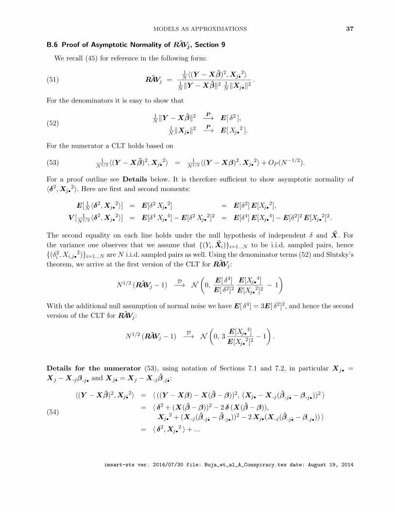
MODELS AS APPROXIMATIONS 37
B.6 Proof of Asymptotic Normality of ˆRAVj, Section 9
We recall (45) for reference in the following form:
(51) ˆRAVj =1N 〈(Y −Xβ)2,Xj•
2〉1N ‖Y −Xβ‖2
1N ‖Xj•‖2
.
For the denominators it is easy to show that
(52)1N ‖Y −Xβ‖
2 P−→ E[ δ2 ],
1N ‖Xj•‖2
P−→ E[Xj•2 ].
For the numerator a CLT holds based on
1N1/2 〈(Y −Xβ)2,Xj•
2〉 = 1N1/2 〈(Y −Xβ)2,Xj•
2〉+OP (N−1/2).(53)
For a proof outline see Details below. It is therefore sufficient to show asymptotic normality of
〈δ2,Xj•2〉. Here are first and second moments:
E[ 1N 〈δ
2,Xj•2〉] = E[δ2Xj•
2] = E[δ2]E[Xj•2],
V [ 1N1/2 〈δ2,Xj•
2〉] = E[δ4Xj•4]−E[δ2Xj•
2]2 = E[δ4]E[Xj•4]−E[δ2]2E[Xj•
2]2.
The second equality on each line holds under the null hypothesis of independent δ and ~X. For
the variance one observes that we assume that {(Yi, ~Xi)}i=1...N to be i.i.d. sampled pairs, hence
{(δ2i , Xi,j•2)}i=1...N are N i.i.d. sampled pairs as well. Using the denominator terms (52) and Slutsky’s
theorem, we arrive at the first version of the CLT for ˆRAVj :
N1/2 ( ˆRAVj − 1)D−→ N
(0,E[ δ4]
E[ δ2]2E[Xj•
4]
E[Xj•2]2− 1
)With the additional null assumption of normal noise we have E[ δ4] = 3E[ δ2]2, and hence the second
version of the CLT for ˆRAVj :
N1/2 ( ˆRAVj − 1)D−→ N
(0, 3
E[Xj•4]
E[Xj•2]2− 1
).
Details for the numerator (53), using notation of Sections 7.1 and 7.2, in particular Xj• =
Xj −X−jβ−j• and Xj• = Xj −X−jβ−j•:
(54)
〈(Y −Xβ)2,Xj•2〉 = 〈 ((Y −Xβ)−X(β − β))2, (Xj• −X−j(β−j• − β−j•))2 〉
= 〈 δ2 + (X(β − β))2 − 2 δ (X(β − β)),
Xj•2 + (X−j(β−j• − β−j•))2 − 2Xj•(X−j(β−j• − β−j•)) 〉
= 〈 δ2,Xj•2 〉+ ...
imsart-sts ver. 2014/07/30 file: Buja_et_al_A_Conspiracy.tex date: August 19, 2014
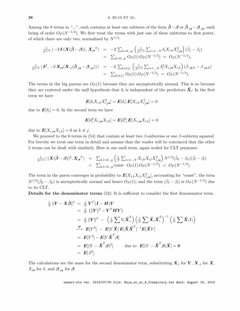
38 A. BUJA ET AL.
Among the 8 terms in “...”, each contains at least one subterm of the form β−β or β−j•−β−j•, each
being of order OP (N−1/2). We first treat the terms with just one of these subterms to first power,
of which there are only two, normalized by N1/2:
1N1/2 〈−2 δ (X(β − β)), Xj•
2 〉 = −2∑
k=0...p
(1
N1/2
∑i=1...N δiXi,kX
2i,j•
)(βj − βj)
=∑
k=0...p OP (1)OP (N−1/2) = OP (N−1/2),
1N1/2 〈 δ2, −2Xj•(X−j(β−j• − β−j•)) 〉 = −2
∑k(6=j)
(1
N1/2
∑i=1...N δ
2iXi,j•Xi,k
)(β−j•,k − β−j•,k)
=∑
k(6=j) OP (1)OP (N−1/2) = OP (N−1/2).
The terms in the big parens are OP (1) because they are asymptotically normal. This is so because
they are centered under the null hypothesis that δi is independent of the predictors ~Xi: In the first
term we have
E[δiXi,kX2i,j•] = E[δi]E[Xi,kX
2i,j•] = 0
due to E[δi] = 0. In the second term we have
E[δ2iXi,j•Xi,k] = E[δ2i ]E[Xi,j•Xi,k] = 0
due to E[Xi,j•Xi,k] = 0 as k 6= j.
We proceed to the 6 terms in (54) that contain at least two β-subterms or one β-subterm squared.
For brevity we treat one term in detail and assume that the reader will be convinced that the other
5 terms can be dealt with similarly. Here is one such term, again scaled for CLT purposes:
1N1/2 〈 (X(β − β))2,Xj•
2 〉 =∑
k,l=0...p
(1N
∑i=1...N Xi,kXi,lX
2i,j•
)N1/2(βk − βk)(βl − βl)
=∑
k,l=0...p const ·OP (1)OP (N−1/2) = OP (N−1/2).
The term in the paren converges in probability to E[Xi,kXi,lX2i,j•], accounting for “const”; the term
N1/2(βk − βk) is asymptotically normal and hence OP (1); and the term (βl − βl) is OP (N−1/2) due
to its CLT.
Details for the denominator terms (52): It is sufficient to consider the first denominator term.
1N ‖Y −Xβ‖
2 = 1N Y
T (I −H)Y
= 1N
(‖Y ‖2 − Y THY
)= 1
N ‖Y ‖2 −
(1N
∑Yi ~X
T
i
)(1N
∑~Xi
~XT
i
)−1 (1N
∑~XiYi
)P−→ E[Y 2] − E[Y ~X]E[ ~X ~X
T]−1E[ ~XY ]
= E[Y 2]−E[Y ~XTβ]
= E[(Y − ~XTβ)2] due to E[(Y − ~X
Tβ) ~X] = 0
= E[ δ2].
The calculations are the same for the second denominator term, substituting Xj for Y , X−j for X,
Xj• for δ, and β−j• for β.
imsart-sts ver. 2014/07/30 file: Buja_et_al_A_Conspiracy.tex date: August 19, 2014
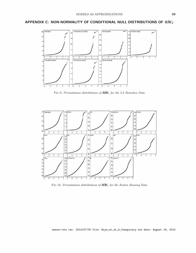
MODELS AS APPROXIMATIONS 39
APPENDIX C: NON-NORMALITY OF CONDITIONAL NULL DISTRIBUTIONS OF ˆRAVJ
Fig 9. Permutations distributions of ˆRAVj for the LA Homeless Data
Fig 10. Permutations distributions of ˆRAVj for the Boston Housing Data
imsart-sts ver. 2014/07/30 file: Buja_et_al_A_Conspiracy.tex date: August 19, 2014