Subodh Kumar Dept of Computer Sc. & Engg. IIT Delhi

Computer Graphics

Subodh Kumar

Dept of Computer Sc. & Engg. IIT Delhi

Shapes! Triangles

! Hard to model, Easy to render (rasterize)! Verbose: too many triangles may be required

! Triangles can be “smoothed”! e.g., subdivision surfaces

! Not a ‘flat’ surface! Curves (hair, grass, fur)! Volumetric elements or particles (cloud, smoke, fire)! More

! Distance-field, Points/Surfels/Splats, Blobs, Sprites, Light-field

Triangles are convenient but generally inefficient ways to represent shape. While the graphics hardware focusses mainly on the common denominator — points, lines, and triangles — models and shapes do not have to be designed that way. Higher level representations are more compact and have more accuracy. They look fine even up close, when the camera zooms in.

Curve/Surface Modeling! Locally flat

! Tangent line/plane at each point! Sometimes higher degree of continuity may be enforced

! Multiple pieces may be stitched together to form the complete shape

! as with triangle meshes! Tangents need not be defined at joints

! Implicit representation! Parametric representation! Subdivision surfaces ! Constructive solid geometry! Distance field

We focus on higher order curve and surface modeling in this lesson. (We will also see that that many mechanisms are common to curves and surfaces — curves proceed in one ‘direction,’ surfaces proceed in two. Looked another way, a surface is many curves.) The following slides introduce some common techniques, and go in some depth on parametric representation.






and other representations ..







Often tiled with triangles for rendering







Often tiled with triangles for renderingBut also recall tessellation shader

Implicit Representation

Point [x,y,z] is on the curve/surface if f(x,y,z) = 0.

f(x, y, z) = 0

x2 + y2 + z2 − 1 = 0e.g.,

x2 + y2 − 1 = 0

If f(x,y,z) ≠ 0, [x,y,z] is not on the curve/surface.

Testing is easy. But enumerating all points is hard. Can be rasterized by finding intersection with scan line.

Implicit representation is based on a general function of the coordinates.

Parametric Representation! Some known range of parameters is taken

! Called the domain! Usually two parameters for a surface

! Call them u and v with, say, 0≤u≤1, and 0≤v≤1! usually one parameter is employed for a curve

! A vector function of the parameters defines the shape

! Easy to enumerate points on the shape by enumerating points in the domain and computing S (or C)! Easy to tile with triangles

S(u, v) ≡ x(u, v), y(u, v), z(u, v)C(t) ≡ x(t), y(t), z(t)Or,

Parametric representation sees the coordinates themselves as functions of some abstract parameter.

Parametric Representation

Can these parameters be useful for texturing?

uv

0,0

t0 1

The parameter domain is shown in white (on a number line for t, or a cross-product of number-lines for (u,v). Each point on the domain is mapped by the parametric function to an x,y,z (which gives a point lying on the curve or the surface, respectively). In this scheme, it is easy to find nearby points on the surface (by taking nearby points on the domain). Also recall texture coordinates. Texture coordinates can be related to these parameters (t, u, or v).

Subdivision SurfaceTriangle Mesh

Subdivision surfaces start with a triangle mesh. (Subdivision curves start with a poly-line.) Local operators on vertices and edges, then produce more detailed mesh. They can represent smooth surfaces (and curves).

There are many subdivision schemes, which converge to different surface for the same starting mesh (also called base mesh, or control mesh). Different schemes have different guarantees of smoothness and relationship to the base mesh. Common schemes include Catmull-clark, Doo-sabin, Loop, Butterfly, etc.


Introduce new vertices Positions are weighted average of old vertices The old vertices may also be shifted similarly ‘Smoothes’ edges and vertices (but sharp edges can also be retained)

Subdivide



Subdivide Subdivide



Subdivide Subdivide

! Can repeat ‘indefinitely’! Converges to a smooth surface

! Smoothness depend on the weights



Subdivide Subdivide

! Can repeat ‘indefinitely’! Converges to a smooth surface

! Smoothness depend on the weights

Constructive Solid Geometry

S1 (Sphere)

S2 (Cylinder)

S1 ⋂ S2 would be just the hole part in this case

CSG starts with some base shapes (which may be simple primitives like cubes, spheres, and cylinders, or more complex shapes designed using one of the other mechanisms).

Set operations on these primitives — rather an expression comprising set operation — then provide the final shape. CSG are a bit harder to control than other methods for free-form design, but are quite useful for engineering objects, and readily provide sharp edges and smooth areas. They also can encode the engineering/manufacturing schema.

The example in the figure shows a cylinder being subtracted from a sphere. The basic operation in CSG is to find curves of intersection between two surfaces. Set Union, Difference, and Intersection can all be described in terms of these intersection curves (and parts of the primitive surfaces).


S1 (Sphere)

S2 (Cylinder)

S1 - S2 (Transformed to bring together)



S1 (Sphere)

S2 (Cylinder)


=

Cylinder removed from sphere



S1 (Sphere)

S2 (Cylinder)


=

Cylinder removed from sphere

Down the barrel view

=


Distance Field

2D Field Dark color indicates small distance Light color indicates large distance

The analytical form of the field function d is not always known. At times, it can only be evaluated at given locations [x, y, z]. Even if the values are known only at certain locations, the curve or surface can be located.

x

y

Distance fields are based on some implicit function (these implicit functions are continuous and directly provide distances from the surface or curve). Sometimes, the distance functions are known on a 3D grid of locations. Such ‘sampled’ distance fields are also called volumes (with each value being referred to as voxel). The rest of the field can be interpolated/reconstructed from these samples.

Distance Field

2D Field Dark color indicates small distance Light color indicates large distance

The 2D field represents this curve

The analytical form of the field function d is not always known. At times, it can only be evaluated at given locations [x, y, z]. Even if the values are known only at certain locations, the curve or surface can be located.

x

y

! Analytic Function! Parametric form: C(t)! Implicit form: F(t) = 0

! Design based on known or desired points! Curve should pass near or through these

Curves to Fit Data

We will now focus on parametric representation and design of parametric curves, with the help of a given sequence of data-points. This curve does not pass through (all) data-points, but it is near them. Hence, it’s called an approximating curve.

! Analytic Function! Parametric form: C(t)! Implicit form: F(t) = 0

! Design based on known or desired points! Curve should pass near or through these

Curves to Fit Data

known points

Approximating curve

curve interpolates this data point

(aka data-points)

Representation Desirables! Stable

! Small changes to data points should induce small change to the curve

! Smooth! Tangent should be continuous! Or, second derivative should be continuous! Second derivative is related to curvature

! Curvature indicates how fast curve turns! Easy to evaluate

! including derivatives, curvature, etc.! Can interpolate or just approximate the data

Parametric FormSuppose curve C is a polynomial in t

P(t) =n

∑k=0

(cktk)i.e., Point P(t) on curve C is computed as follows:

ck are vector coefficients (with x, y, z coordinates)

All data points satisfy the above equation. If the number of data points is (n+1), ⇒ (n+1) unknown ck can be computed using (n+1) linear equations.

(For each coordinate)

Interpolating curve

Remember the parametric form allows computation of each coordinate — each is an independent function of the parameter. We interpret the coefficients as vectors. It may be easier to think of one of the coordinates, say y (for both P and c).

Parametric FormSuppose curve C is a polynomial in t

P(t) =n

∑k=0

(cktk)i.e., Point P(t) on curve C is computed as follows:

ck are vector coefficients (with x, y, z coordinates)

All data points satisfy the above equation. If the number of data points is (n+1), ⇒ (n+1) unknown ck can be computed using (n+1) linear equations.

(For each coordinate)

Interpolating curve

We do not have to use this form. Other forms are possible, we will see.

Interpolating Curve

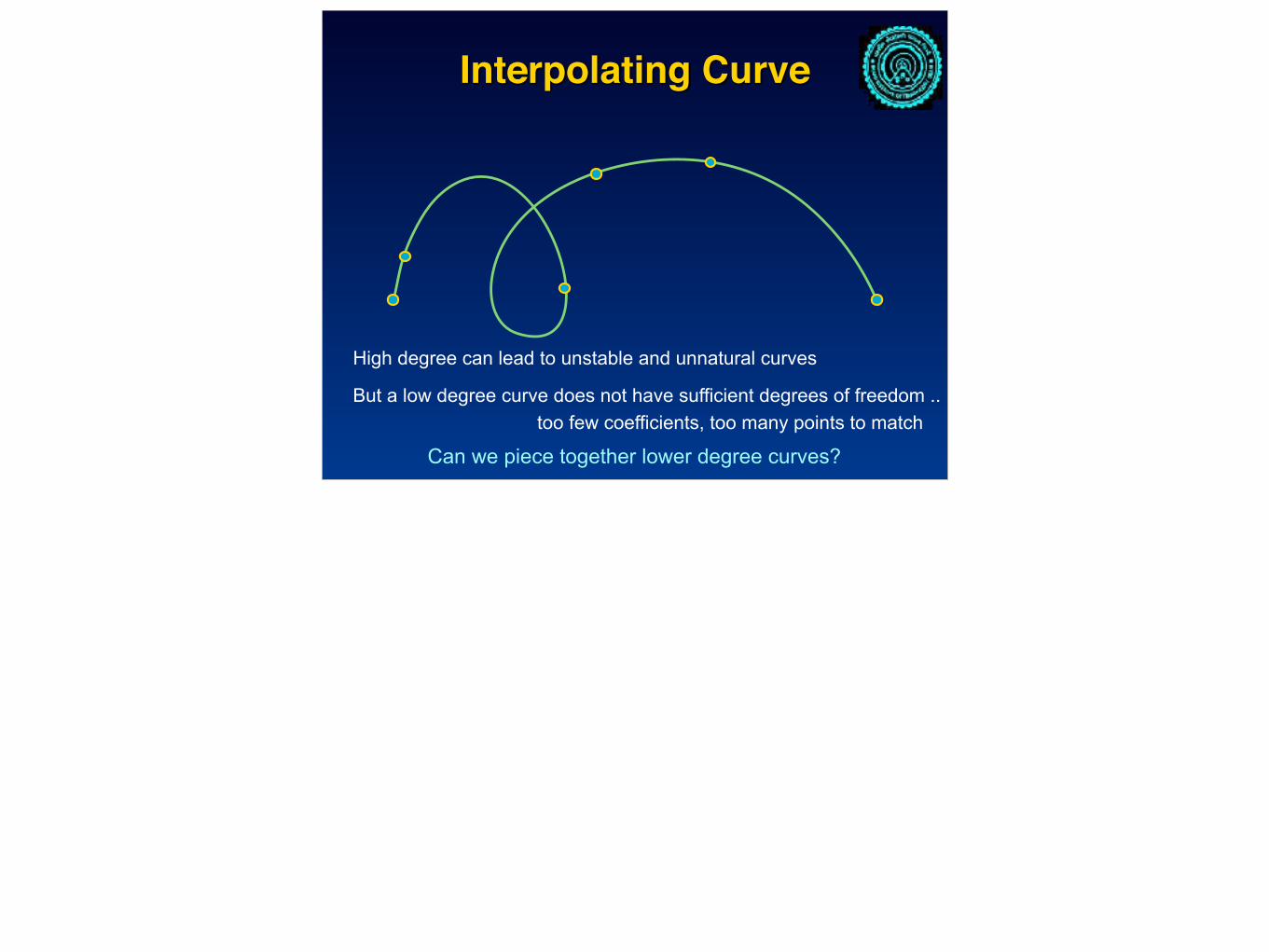
High degree can lead to unstable and unnatural curves

We want to have many lower degree curves combine to form the overall curve.

Interpolating Curve


But a low degree curve does not have sufficient degrees of freedom .. too few coefficients, too many points to match

Interpolating Curve


But a low degree curve does not have sufficient degrees of freedom .. too few coefficients, too many points to match

Can we piece together lower degree curves?

Matrix Form for Cubics

[c] =

c0c1c2c3

[t] =

1tt2

t3

P(t) =3

∑k=0

(cktk)

P(t) = [t]⊤[c] = [c]⊤[t]

Consider cubic curve, n = 3:

Let,

⇒

Sometimes it is convenient to express the equations in terms of matrices. We will assume the coefficients and powers of the parameter are written as column vectors. Each parametric scheme then can be specified by its matrix.

Documents

Subodh Kumar Dept of Computer Sc. & Engg. IIT Delhi