Embed Size (px)
Citation preview
Subproblem Sampling-based Stochastic Programming Method
for Power Systems Planning and Operations Problems
Nahal Sakhavand1 and Harsha Gangammanavar2
1Department of Industrial Manufacturing and Systems Engineering, University of Texas
at Arlington, Arlington, TX-76010, USA2Department of Engineering Management, Information, and Systems, Southern
Methodist University, Dallas, TX-75275 USA
October 22, 2020
Abstract
In this paper, we present a two-stage stochastic programming and simulation-based framework
for tackling large-scale planning and operational problems that arise in power systems with signifi-
cant renewable generation. Traditional algorithms (the L-shaped method, for example) used to solve
the sample average approximation of the true problem suffer from computational difficulties when
the number of scenarios or the size of the subproblem increases. To address this, we develop a cut-
ting plane method that uses sampling internally within optimization to select only a random subset
of subproblems to solve in any iteration. We analyze the convergence property of the subproblem
sampling-based method and demonstrate its computational advantages on two alternative formu-
lations of the stochastic unit commitment-economic dispatch problem. We conduct the numerical
experiments on modified IEEE-30 and IEEE-118 test systems. We also present detailed steps for
assessing the quality of solutions obtained from sampling-based stochastic programming methods
and determining a solution to prescribe to the system operators.
1 Introduction
Over the past couple of decades, there has been a significant increase in the share of energy generated
from renewable resources in energy portfolios around the world. New capacity addition in renewable
resources outpaced capacity addition in conventional energy resources by a factor of five [14]. These new
capacity additions have largely been in solar and wind resources which are often classified together as
intermittent energy resources. Their growth can be attributed not only to the environmentally friendly
characteristics but also to the fact that they have now become economically viable when compared to
conventional resources like coal and nuclear [27].
1
Sakhavand and Gangammanavar Subproblem Sampling-based SP Method
However, a large-scale installation of renewable resources, particularly wind and solar, has brought
forth the new challenges associated with operating the power grid. This is related to the two inherent
characteristics of these resources uncertainty and intermittency. The stochasticity in renewable gener-
ation concerns with its dependence on environmental conditions such as temperature, humidity, cloud
cover, etc. This makes predicting the amount of generation from these resources notoriously difficult.
The intermittency on renewable resources, on the other hand, pertains to the inability to maintain con-
tinuous generation from these resources. It is also closely related to the large fluctuation in generation
over short periods.
One of the principal power systems planning components is the Unit Commitment (UC) problem
where the operating schedule for generators is determined. Several formulations and solution method-
ologies have been proposed for the UC problem that include dynamic programming and Mixed Integer
Linear Programming (MILP). Another critical planning component is the Economic Dispatch (ED)
problem where generation quantities of the scheduled generators are determined to ensure the balance
between supply and demand. The ED problem is also formulated as an optimization problem (often as
a linear program) that considers the topology of the power network. To the best of our knowledge, the
current practice at system operators is to use a single point forecast of demand and renewable generation
in the UC and ED problems. This results in deterministic instances of these optimization problems that
can be solved using off-the-shelf deterministic solvers.
In order to accommodate the challenges introduced by integration of the renewable resources, new
features such as increasing generation flexibility using fast-ramping operating reserves, demand-side
management, and storage devices have been incorporated. In addition to these features, there has been
a growing interest in migrating from deterministic optimization to more robust stochastic optimization
tools to solve the UC and ED problems. While there are clear advantages of using stochastic optimization,
their acceptance by power system operators is incumbent upon the availability of reliable algorithms that
scale graciously to large-scale applications.
Decomposition-based stochastic programming (SP) models, particularly two-stage stochastic linear
programs (2-SLP) with expectation-valued objective function, have proven to be very effective to model
UC and ED problems. In these models, the first-stage corresponds to the decisions made before an
observation of uncertainty and the second-stage allows for recourse actions that can be taken after the
observation. Such a modeling approach provides a convenient tool to capture the complicated operational
relationships such as minimum uptime/downtime requirements, nonlinear startup cost, etc. The first
stochastic UC (S-UC) model is proposed in [31] which considers uncertainty in demand. In recent years,
there have been a significant number of works that study S-UC with uncertainty in renewable generation
such as wind and solar generation. We refer the interested reader to [34] for a comprehensive review of
these works. Stochastic ED (S-ED) has been addressed using a deterministic equivalent form in [16], a
probabilistic approach in [22], and a two-stage decomposition-based method in [7]. In several works (e.g.,
[2] and [30]), the UC problem is formulated as a first-stage program and the ED problem is included in the
second-stage to capture dispatch in response to observations of demand and renewable uncertainty. In SP
models for UC and ED, it is critical to use an appropriate representation of the underlying uncertainty
2
Sakhavand and Gangammanavar Subproblem Sampling-based SP Method
corresponding to renewable generation and demand. Such a representation is achieved by modeling them
as continuous random variables. In this case, the computation of expectation-valued objective function
involves multiple integrals, and therefore, approximate uncertainty representations must be employed. A
popular approach is to consider a finite set of scenarios that are generated using Monte Carlo simulation
approaches. The resulting optimization problem is referred to as the sample average approximation
(SAA) problem [26]. This approach has been used for S-UC problems. For example, in [29] a sample
of 10 scenarios and in [17] samples of sizes {50, 100, 200} scenarios are used to set up the SAA. It is
worthwhile to note that, once the sample is generated, the SAA problem is a deterministic optimization
problem. In [29] and [17], the deterministic Benders decomposition is used as a solution procedure, albeit
with a small number of scenarios.
The use of SAA is supported by strong theoretical backing. SAA is a consistent estimator of the
original SP problem and exhibits an exponential rate of convergence (see Chapter 5 in [26] for detailed
results). For problems involving discrete decision variables, which is the case in UC and ED problems,
the asymptotic analysis of SAA is first conducted in [13]. While SAA provides asymptotic guarantees,
the behavior of solutions obtained using a finite sample must be carefully assessed. Since a random
sample is used to set up the SAA, the optimal value and the solution obtained by solving the SAA are
stochastic. Therefore, a multiple replication-based approach is proposed in [18] which has been applied to
assess the empirical behavior of SAA on several SP instances in [15]. Both the theoretical and empirical
results indicate that increasing the number of samples used to generate the SAA will (i) reduce bias (the
expected difference between the SAA and the true SP models’ optimal values) and (ii) reduce variance
across the replications. The two features can be viewed as certificates of quality and reliability of SP
solutions, respectively. Unfortunately, using large sample sizes and multiple replication procedures can
be computationally prohibitive for large-scale S-UC and S-ED problems.
A popular approach to address this computational difficulty is to employ scenario reduction techniques
that reduce the original sample to a smaller subset of manageable size. These techniques are based on
stability analysis of SP models and use probability metrics to identify “similar” scenarios and remove
them from the original sample. In power systems applications, the use of the scenario reduction technique
proposed by [4], particularly the faster variant developed by [9], is very common. This technique is based
on the Kantorovich metric of probability distributions that takes into account the difference in the
random vectors. For example, in [32] scenario reduction from 100 to 10 scenarios is used to compute
commitment decisions and in [19] a sample of size 3018 is reduced to 20 to evaluate the economic value
of the reserves. A scenario reduction technique that matches certain statistics (for e.g., moments) of the
original and reduced scenario was proposed in [12] and adopted in a reserve requirement problem in [24].
The techniques discussed so far operate only in regards to the observations of the random vector and the
associated probabilities are impervious to the decision problem. In other words, these scenario reduction
techniques do not account for the impact of observations on the optimization outcome (optimal solution
and value).
In [20], the authors use a similar approach to [4], but instead of using the difference in observations,
they use the objective function value of the second-stage problem associated with the observations. A
3
Sakhavand and Gangammanavar Subproblem Sampling-based SP Method
similar approach is used in [5] where observations are clustered based on the optimal objective func-
tion values, and then use the scenario reduction algorithm of [9] within each cluster. An important
sampling-based approach is used in [23] for selecting scenarios for the S-UC problem. In these ap-
proaches, computations necessary for scenario reduction/selection is performed at a particular first-stage
decision variable (often the optimal solution of the mean-value problem). The decomposition-based SP
methods generate a sequence of first-stage solutions which converge to the optimal solution. The efficacy
of the reduced set is not necessarily the same across all solutions in the sequence, and hence, the scenario
reduction techniques are mere heuristics without any solution quality guarantees on bias or variance.
In light of these observations, the main contribution of this paper are as follows:
1. We present a two-stage SP modeling and simulation framework for stochastic unit commitment-
economic dispatch (S-UCED) that includes the UC problem in the first-stage and the ED problem
in the second-stage. We consider two alternative formulations for the UC problem proposed in
[21] and [1]. Our S-UCED model captures uncertainty in renewable generation whose scenarios
are simulated using statistical time series models. An additional simulation feature is incorporated
to enable efficient subproblem sampling (see (2) below). This framework inherits the merit of SP
models to outperform conventional models by providing more realistic solutions.
2. We present a cutting-plane SP algorithm with subproblem sampling designed specifically to solve
S-UCED problems. There are two main advantages of the subproblem sampling-based approach.
(i) It solves the original SAA problem to optimality in finite number of iterations. Thereby, retains
the statistical properties of SAA such as a reduction in bias and variance with an increase in
sample size. (ii) It significantly improves the computational performance over the SAA approach.
In fact, its computational effort is comparable to what is required to solve the optimization problem
obtained after scenario reduction.
3. We conduct comprehensive computational experiments to study the performance of our cutting-
plane SP algorithm. We contrast the solutions obtained using our algorithms to those obtained by
solving full sample SAA problems to assess the solution quality. We demonstrate the computational
performance of our approach to the well-accepted scenario reduction technique using the fast-
forward algorithm of [9]. The experiments are conducted on standard power systems instances
from the literature.
The remainder of the paper is organized as follows. In section 2, we present the S-UCED problem
formulations used in this paper. Next, we proceed with the detailed subproblem sampling-based cutting-
plane method in section 3. We discuss the results of our computational experiments in section 4, and
finalize the paper with the conclusion in section 5.
2 Problem Formulation
The principal idea of subproblem sampling-based cutting-plane method is suitable for general two-stage
stochastic programs (2-SPs) which are applicable for a wide range of problems arising in power systems
4
Sakhavand and Gangammanavar Subproblem Sampling-based SP Method
planning and operations. Due to the relative importance of the S-UCED problem, and the availability of
standard test instances, we use this problem to illustrate the potential of our approach. When we have
linear programs in both the stages, which is the case in the S-UCED problems, we can state the 2-SP in
the following general form:
min f(x, z) := c(x, z) + E{Q(x, z, ξ)} (1a)
s.t (x, z) ∈ X := {(x, z) | A[x; z] = b} ⊆ Rn1+ × Bm1 .
Here, the recourse function is the optimal value of the following program:
Q(x, z, ξ) = min d(y, ξ) (1b)
s.t Wy = r(ξ)− T [x; z], y ∈ Rn2+ .
The first-stage decision z includes the binary commitment decisions and x captures the continuous
decision variables in the UC problem. The second-stage program is solved for a given set of first-stage
decisions (x, z) and a realization ξ of the random vector ξ. We assume that the random vector is
defined over the probability space (Ξ,F , P ), and is used to model uncertainty in demand and renewable
generation over the horizon of the problem. The second-stage dispatch decisions are captured by the
vector y.
2.1 Unit Commitment
We consider two alternative formulations of the UC problem that were originally proposed in [21] and [1].
We refer to these formulations as MLR and ALS, respectively, after the initials of their corresponding
authors. Our ED model is based on [7]. We study a two-stage multi-period S-UCED framework where
uncertainty is due to the inclusion of renewable generation. In the following we only discuss the main
differences between the two formulations and defer the detailed presentation to the appendix B.
Both the UC formulations use three binary variables to capture the status of a generator at any time
period t. These decisions appear as vector z in (1a). In MLR, at any time period t, these binary variables
take a value of 1 if (1) the generator is on, (2) the generator is turned on, and (3) the generator is turned
off in time period t, respectively. On the other hand, in ALS, the first binary variable is defined as a
state-transition variable and is considered to be 1 if the unit remains operational and 0 otherwise. The
use of state-transition variables, as opposed to the commitment decision variables in MLR, enables a
network sub-structure in the UC problem formulation that provides certain computational advantages
(see [1] and references therein for detailed discussions in the deterministic setting).
Both the formulations capture the critical operational requirements of the UC problem. These include
• Minimum uptime and downtime requirement;
• Ramp-up/down and minimum start up/shut down generation requirements;
• Generation capacity restrictions; and
• Start-up costs that depend on the generators’ idle time.
5
Sakhavand and Gangammanavar Subproblem Sampling-based SP Method
In the 2-SP setting of S-UCED, the UC decision is made before the realization of uncertainty. At
this stage, requirements pertaining to transmission, power flows, etc. are often excluded. In turn, a
system-wide requirement is included that mandates that the system-wide expected net-demand (expected
demand minus expected renewable generation) is met by committed generation. In order to accommodate
the possibility of deviating from the committed generation, once the actual demand and renewable
generation is realized, supplementary generation or reserve capability needs to be committed. The
MLR and ALS formulations capture these requirements differently. The MLR formulation addresses
this requirement by including additional spinning reserve decision variables. The committed generation
and the spinning reserve together constitute the continuous decision vector x in (1a). On the other
hand, in the ALS the vector x comprises of the generation amount above the minimum capacity and
maximum generation after adjusting for uncertainty (first introduced in [3]). The subtle differences in
these alternative approaches to formulate the UC problem result in model instances that differ both in the
computational performance as well as solution quality. We discuss these differences in our experimental
study (§4).
2.2 Economic Dispatch
Once our commitment and reserve decisions are established in the first-stage, we determine the dispatch
decisions that include actual generation, power flows, and phase angle for all time periods considered
in the ED problem horizon. The formulation for the ED problem is adopted from [7]. These variables
constitute the second-stage decision vector y in (1b). The hour-ahead generation cost represented in
function d(·) is a piece-wise linear convex function of the dispatch amounts. The load shedding and
generation curtailment penalties are also embedded in d(·). The constraints included in the ED problem
include the following.
• The flow balance constraints which guarantees the conservation of energy at every bus in the
network.
• Generation capacity restrictions and ramp-up/down requirements.
• Power flow equations. We use the DC linear approximation of the power flow that ignores reactive
power and assumes second-order terms to be negligible.
• Bounds on bus phase angles, availability of renewable generation, and demand.
The stochastic elements in the ED problem correspond to demand and renewable generation. These
terms appear on the right-hand side (r(ξ)) of the equality constraints in (1b). We refer the reader to the
B for the full model description.
6
Sakhavand and Gangammanavar Subproblem Sampling-based SP Method
3 Solution Method
Let us consider the SAA of (1) constructed using a sample Ξn ⊆ Ξ of n demand and renewable generation
scenarios. The first-stage objective can then be stated as
min(x,z)∈X
fn(x, z) := c(x, z) +1
N
n∑j=1
Q(x, z, ξj). (2)
For problems with finite support, such as (2), the L-shaped method [28] has been very effective as a
solution approach. In this method, a lower bounding approximation is constructed using a collection
of affine functions (cuts). The computation of these affine functions involves solving the second-stage
subproblem corresponding to all observations in Ξn to optimality, herein lies the computational bottleneck
of the method. To alleviate this, we present the notion of subproblem sampling and introduce it within
a cutting-plane method.
We begin by stating the assumptions on the SAA in (1).
(A1) For any UC feasible decision (x, z) and observation ξ ∈ Ξn, there exists a feasible ED decision.
(A2) The dual feasible set of (1b) is non-empty.
(A3) The uncertainty only affects the right-hand side parameters in (1b).
Assumption (A1) is often referred to as the relatively complete recourse, which is satisfied by S-UCED if
we allow for load-shedding and generation curtailment. Since the ED costs have a trivial lower bound of
zero, assumption (A2) is satisfied. Finally, the demand and renewable generation affect only the right-
hand side of the flow balance equations corresponding to the connected buses. Therefore, assumption
(A3) is satisfied for S-UCED problems. This implies that the 2-SP model of S-UCED has a fixed recourse
(i.e., matrix W is deterministic). Assumptions (A1) and (A2) together imply that the dual feasible set
in bounded and the recourse value −∞ < Q(x, z, ξ) <∞, for all (x, z) ∈ X almost surely.
The dual of the ED problem in (1b) under assumptions (A1)–(A3) is given by
max π>(r(ξ)− T [x; z]) (3)
s.t. π ∈ Π := {π | W>π ≤ d′(y)}.
Notice that the dual feasible set is a polytope that is not affected by the randomness or the first-stage
decision (x, z). We denote the set of dual basic feasible solutions by Π. Linear programming duality
ensures that any π ∈ Π satisfies Q(x, z, ξ) ≥ π>(r(ξ) − T [x; z]) for all (x, z) ∈ X and ξ ∈ Ξ. This
observation motivates our subproblem sampling approach.
3.1 Subproblem Sampling-based Cutting-plane Method
We describe the steps of the algorithm in iteration k. At the beginning of the iteration, we have an
approximation of the first-stage objective function fkn(x, z) defined using the set of affine functions
J k−1, and a set of dual vertices discovered by the algorithm Πk−1. The iteration begins by solving the
7
Sakhavand and Gangammanavar Subproblem Sampling-based SP Method
master problem to identify a candidate solution:
(xk, zk) ∈ argmin {c(x, z) + fkn(x, z) | (x, z) ∈ X}. (4)
Let Ek denote a subset of observations obtained using Bernoulli sampling from the finite set Ξn.
That is, every observation ξ ∈ Ξn is subjected to an independent Bernoulli trial with a given probability
p ∈ [0, 1]. For every ξ ∈ Ek, we set up and solve the subproblem Q(xk, zk, ξ). The πk(ξ) denote
the optimal dual solution obtained is added to the collection of previously discovered dual vertices:
Πk = Πk−1 ∪ {πk(ξ)}ξ∈Ek . For observation ξ ∈ Ξn \ Ek, the best dual vertex is identified from the
collection Πk using the “argmax” procedure
πk(ξ) = argmax{π>(r(ξ)− T (ξ)xk|π ∈ Πk}. (5)
The use of the argmax procedure above is inspired by its use in the stochastic decomposition algorithm
[10]. In essence, for observations in the subset Ek an optimal dual solution is obtained by solving
the subproblem to optimality and for those not included in the subset, the argmax procedure in (5) is
employed to identify a suboptimal dual solution.
Using the set of dual solutions, we can then compute the affine function coefficients as follows:
αk = πk(ξi)>r(ξi); βk = (−T (ξi))>πk(ξi). (6)
This affine function is added to the collection J k−1 to obtain J k. Using the latest affine function, the
first-stage objective function is updated as follows:
fkn(x, z) = maxj∈J k
{αj + (βj)>[x; z]}. (7)
This completes one iteration of the algorithm. The complete algorithm is presented in Algorithm 1.
In the L-shaped method, subproblems associated with all the observations are solved in every iter-
ation which can be achieved in Algorithm 1 by setting p = 1. In this sense, the subproblem sampling
algorithm generalizes the standard L-shaped method. Further, since the subset Ek is a random sample,
the coefficients in (6) are stochastic in nature. This marks a significant deviation from the deterministic
coefficients generated in the L-shaped method which are deterministic.
The subproblem sampling-based cutting-plane method presented in Algorithm 1 is designed with an
eye to improve the computational time while retaining optimality guarantees. The following proposition
identifies the convergence of the algorithm.
Proposition 3.1. Under assumptions (A1)–(A3), the subproblem sampling-based cutting-plane Algo-
rithm 1 solves the problem in (2) in finite number of iterations.
Proof. Notice that the dual vertex encountered in an iteration of the algorithm is used to update the set
of dual vertices (Step 9. Therefore, the sequence of sets of dual vertices satisfies: Πk−1 ⊆ Πk ⊆ Πk+1,
for all k ≥ 1. Therefore, the first-stage objective function approximation in (7) satisfies:
fk−1n (x, z) ≤ fkn(x, z) ≤ fk+1n (x, z)
8
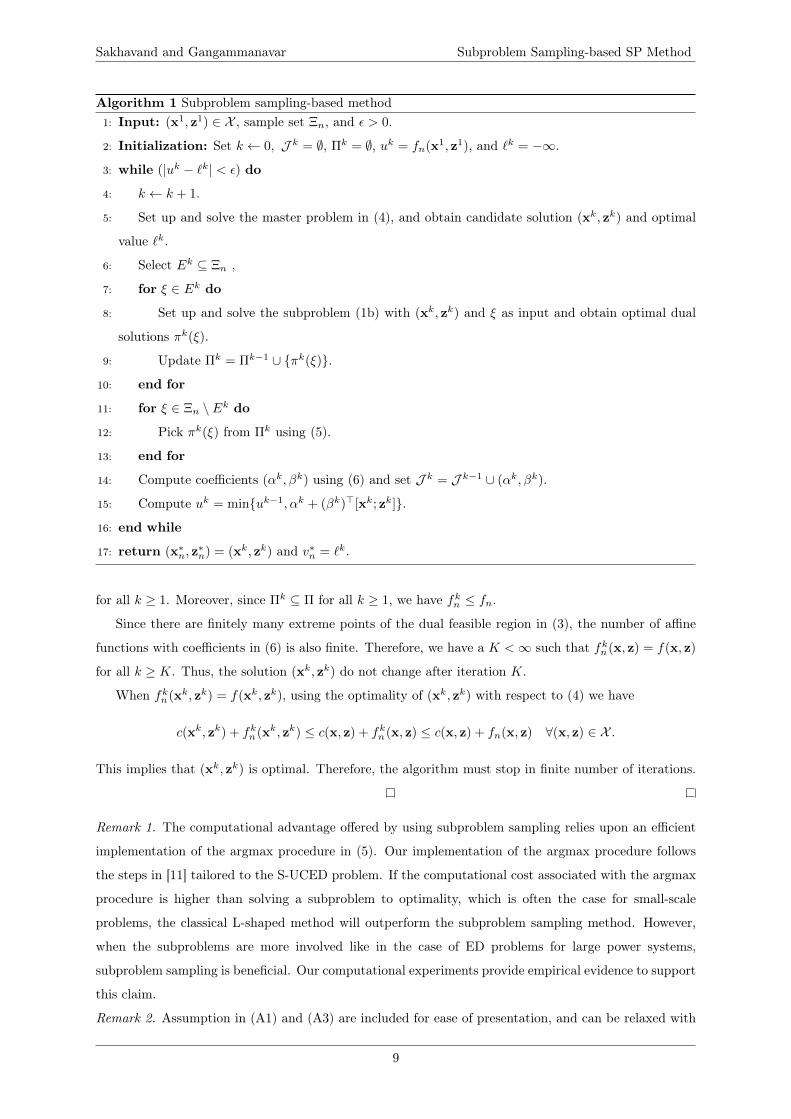
Sakhavand and Gangammanavar Subproblem Sampling-based SP Method
Algorithm 1 Subproblem sampling-based method1: Input: (x1, z1) ∈ X , sample set Ξn, and ε > 0.
2: Initialization: Set k ← 0, J k = ∅, Πk = ∅, uk = fn(x1, z1), and `k = −∞.
3: while (|uk − `k| < ε) do
4: k ← k + 1.
5: Set up and solve the master problem in (4), and obtain candidate solution (xk, zk) and optimal
value `k.
6: Select Ek ⊆ Ξn ,
7: for ξ ∈ Ek do
8: Set up and solve the subproblem (1b) with (xk, zk) and ξ as input and obtain optimal dual
solutions πk(ξ).
9: Update Πk = Πk−1 ∪ {πk(ξ)}.
10: end for
11: for ξ ∈ Ξn \ Ek do
12: Pick πk(ξ) from Πk using (5).
13: end for
14: Compute coefficients (αk, βk) using (6) and set J k = J k−1 ∪ (αk, βk).
15: Compute uk = min{uk−1, αk + (βk)>[xk; zk]}.
16: end while
17: return (x∗n, z∗n) = (xk, zk) and v∗n = `k.
for all k ≥ 1. Moreover, since Πk ⊆ Π for all k ≥ 1, we have fkn ≤ fn.
Since there are finitely many extreme points of the dual feasible region in (3), the number of affine
functions with coefficients in (6) is also finite. Therefore, we have a K <∞ such that fkn(x, z) = f(x, z)
for all k ≥ K. Thus, the solution (xk, zk) do not change after iteration K.
When fkn(xk, zk) = f(xk, zk), using the optimality of (xk, zk) with respect to (4) we have
c(xk, zk) + fkn(xk, zk) ≤ c(x, z) + fkn(x, z) ≤ c(x, z) + fn(x, z) ∀(x, z) ∈ X .
This implies that (xk, zk) is optimal. Therefore, the algorithm must stop in finite number of iterations.
Remark 1. The computational advantage offered by using subproblem sampling relies upon an efficient
implementation of the argmax procedure in (5). Our implementation of the argmax procedure follows
the steps in [11] tailored to the S-UCED problem. If the computational cost associated with the argmax
procedure is higher than solving a subproblem to optimality, which is often the case for small-scale
problems, the classical L-shaped method will outperform the subproblem sampling method. However,
when the subproblems are more involved like in the case of ED problems for large power systems,
subproblem sampling is beneficial. Our computational experiments provide empirical evidence to support
this claim.
Remark 2. Assumption in (A1) and (A3) are included for ease of presentation, and can be relaxed with
9
Sakhavand and Gangammanavar Subproblem Sampling-based SP Method
minimal additional effort. In the absence of complete recourse, we may encounter candidate solutions
(xk, zk) which may be infeasible for some observations in ξ ∈ Ek. This can be handled by generating
feasibility cuts, similar to the L-shaped method. When the dispatch costs are random (see [32] and [33],
for example), the dual feasible set is affected by randomness. Therefore, the argmax procedure must be
carefully redesigned to account for randomness. This can be done based on the steps presented in [6].
Both these features have been included in our implementation of the algorithm.
3.2 Solution Quality Assessment
The solutions obtained by the procedure in Algorithm 1 are stochastic in nature due to the use of the
random sample Ξn. Therefore, the solutions should not is accepted without posterior analyses.
From the SAA theory, we have E[v∗n] ≤ v∗, where v∗N and v∗ are the optimal objective function
values for the SAA problem and the true problem (1), respectively. In order to obtain an estimate of
E[v∗n], we adopt the multiple replication procedure presented in [18] to assess the quality of the solutions.
Let M denote the number of replications. Let (x∗,mn , z∗,mn ) and v∗,mn denote the optimal solution and
value, respectively, obtained by solving the SAA with random sample Ξmn . Using these the lower bound
estimate and its variance can be calculated as
Ln =1
M
M∑m=1
v∗,mn ; σ2Ln
=1
(M − 1)
M∑m=1
(v∗,mn − Ln). (8)
To obtain an estimate of the upper bound, we note that f(x, z) ≥ v∗ for any (x, z) ∈ X . Using these
we obtain an unbiased estimator of f(·) as
Umn′ = c(x∗,mn , z∗,mn ) +1
n′
n′∑j=1
Q(x∗,mn , z∗,mn , ξj). (9)
Notice that the above estimator uses n′ � n realizations of the random vector that are simulated
independently of the sample used for optimization. Using these estimates computed at solutions obtained
from individual replication, an upper bound estimate can be computed as
Un′ =1
M
M∑m=1
Umn′ (10)
Let σ2Un′ denote the variance of the above estimator. We can also compute the confidence intervals (CI)
at level (1− a) for the estimates in (8) and (10) as
CIL =[Ln ±
ζa/2σL√M
]; CIU =
[Un′ ±
ζa/2σU√M
], (11)
where ζa/2 is the (1− a/2) quantile of the standard normal distribution. Using the CIs computed above,
we define a pessimistic gap as the difference between the upper limit of the CIU and the lower limit of
CIL. If the pessimistic gap is lower than a desired threshold, then we have a statistical guarantee on the
optimal objective function value.
10
Sakhavand and Gangammanavar Subproblem Sampling-based SP Method
4 Numerical Results
In this section, we present the numerical results from our experiments conducted on standard power
systems test instances. To facilitate the discussion, we have identified the following questions of interest.
Q1. Does subproblem sampling alleviate the scale complexity of the algorithm and improve the comput-
ing time when compared to solving instances with the traditional L-shaped method (full sampling)?
Q2. How does subproblem sampling compare with the scenario reduction techniques that are prevalent
in the application of sampling-based SP for power system problems?
Q3. What criteria do we need to follow in order to choose a solution for implementation among the set
of optimal solutions obtained using the replicated process?
In addition to the above questions, we present a comparison between solutions recommended by the two
different S-UCED formulations (MLR and ALS).
We conducted the experiments on modified IEEE-30 and IEEE-118 bus systems. The modified
IEEE30 system has 30 buses along with 6 generators of which 2 of them are solar generators. The
modified IEEE118 bus system has 54 generators of which 36 are conventional and the remaining 18 are
renewable generators. SAA instances were built for both MLR and ALS S-UCED formulations. These
instances were used based on samples of independent and identically distributed scenarios of wind and
solar generation of size n = {50, 100, 200, 500, 1000}. These scenarios were simulated in R using a time
series model. The SAA instances were solved using the L-shaped method implemented on a C/C++
platform using CPLEX 12.9 on a Linux-based server with a processor of 64 GB RAM. The internal
stopping criteria for the L-shaped method was set to ε = 0.01 for the IEEE-30 bus system and ε = 0.05
for the IEEE-118 bus system.
We conduct replicated experiments with M = 30. Across these 30 replications, we compute the lower
bound estimate Ln and the out-of-sample upper bound estimate Un using (8) and (10), respectively.
We also compute the confidence intervals for Ln and Un at a = 5% using (11). While presenting our
results, we will present the lower bound and upper bound estimates along with the half-width of their
confidence intervals. We also report the pessimistic gap and the average computational time with its
standard deviation.
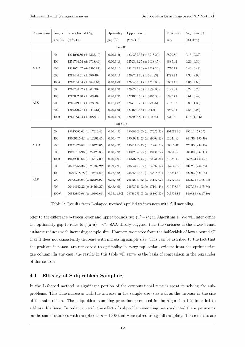
We report the results of the experiments conducted on the SAA instances in Table 1. These results
were obtained using the L-shaped method with a two-hour upper limit on the computational time per
replication. Recall that, in any iteration of the L-shaped method, one subproblem is solved for every
scenario. Therefore, we refer to the results in Table 1 as “full sampling”. Notice that the computational
time increases with the number of scenarios that can directly be attributed to the increased number of
subproblem solves. Due to the large-scale nature of the IEEE-118 problem instances, the best solution
achieved within the time limit is reported. For instance, the experiment with ALS for 1000 scenarios
led to the termination of 4 replications due to the imposed time limit. The table also presents the range
of optimization gaps at the termination of the optimization step. We use the term optimization gap to
11
Sakhavand and Gangammanavar Subproblem Sampling-based SP Method
Formulation Sample Lower bound (Ln) Optimality Upper bound Pessimistic Avg. time (s)
size (n) (95% CI) gap (%) (95% CI) gap (std.dev.)
ieee30
MLR
50 1234056.86 (± 3336.10) [0.00,0.26] 1234332.36 (± 3218.20) 6829.80 0.16 (0.32)
100 1251794.74 (± 1718.46) [0.00,0.18] 1252343.25 (± 1618.45) 3885.42 0.29 (0.30)
200 1234071.27 (± 3290.83) [0.00,0.13] 1234332.36 (± 3218.20) 6770.13 0.46 (0.43)
500 1262444.31 (± 780.46) [0.00,0.10] 1262741.76 (± 694.83) 1772.74 7.30 (2.98)
1000 1253194.94 (± 1546.53) [0.00,0.06] 1253493.31 (± 1516.30) 3361.19 3.05 (4.50)
ALS
50 1266734.22 (± 861.30) [0.00,0.99] 1269225.93 (± 1839.00) 5192.01 0.29 (0.20)
100 1267082.10 (± 869.46) [0.26,0.99] 1271369.52 (± 3765.83) 8922.71 0.54 (0.42)
200 1266419.11 (± 478.18) [0.01,0.89] 1267150.70 (± 979.26) 2189.03 0.89 (1.35)
500 1269229.27 (± 1410.64) [0.00,0.96] 1271640.43 (± 0.00) 3969.94 2.55 (4.93)
1000 1265783.04 (± 308.91) [0.00,0.70] 1268908.80 (± 100.54) 831.75 4.18 (11.36)
ieee118
MLR
50 19045682.61 (± 17616.42) [0.00,4.92] 19098268.00 (± 37376.28) 107578.10 190.11 (55.67)
100 19009715.42 (± 12107.45) [0.00,4.77] 19009243.53 (± 29409.36) 41044.93 244.36 (106.39)
200 19021973.52 (± 16370.05) [0.00,4.99] 19041180.70 (± 31289.23) 66866.47 573.30 (262.03)
500 19021316.96 (± 24325.88) [0.00,4.99] 19042827.98 (± 43434.77) 89271.67 981.09 (567.91)
1000 19032001.64 (± 16217.00) [0.00,4.97] 19070788.43 (± 32931.34) 87935.13 2512.34 (414.78)
ALS
50 20417256.35 (± 21082.2)2 [0.79,4.91] 20684425.88 (± 64392.12) 352643.88 332.21 (244.78)
100 20394778.78 (± 19741.89) [0.02,4.98] 20565529.61 (± 53848.69) 244341.40 722.93 (621.75)
200 20406734.94 (± 22998.97) [0.78,4.98] 20662373.52 (± 74182.92) 352820.47 1373.10 (1388.33)
500 20414142.32 (± 24564.27) [0.48,4.98] 20653011.92 (± 47164.43) 310598.30 2477.38 (1665.36)
1000∗ 20542882.96 (± 19803.66) [0.08,11.50] 20718775.93 (± 48102.20) 243798.83 3449.83 (2147.10)
Table 1: Results from L-shaped method applied to instances with full sampling.
refer to the difference between lower and upper bounds, see (uk−`k) in Algorithm 1. We will later define
the optimality gap to refer to f(x, z) − v∗. SAA theory suggests that the variance of the lower bound
estimate reduces with increasing sample size. However, we notice from the half-width of lower bound CI
that it does not consistently decrease with increasing sample size. This can be ascribed to the fact that
the problem instances are not solved to optimality in every replication, evident from the optimization
gap column. In any case, the results in this table will serve as the basis of comparison in the remainder
of this section.
4.1 Efficacy of Subproblem Sampling
In the L-shaped method, a significant portion of the computational time is spent in solving the sub-
problems. This time increases with the increase in the sample size n as well as the increase in the size
of the subproblem. The subproblem sampling procedure presented in the Algorithm 1 is intended to
address this issue. In order to verify the effect of subproblem sampling, we conducted the experiments
on the same instances with sample size n = 1000 that were solved using full sampling. These results are
12
Sakhavand and Gangammanavar Subproblem Sampling-based SP Method
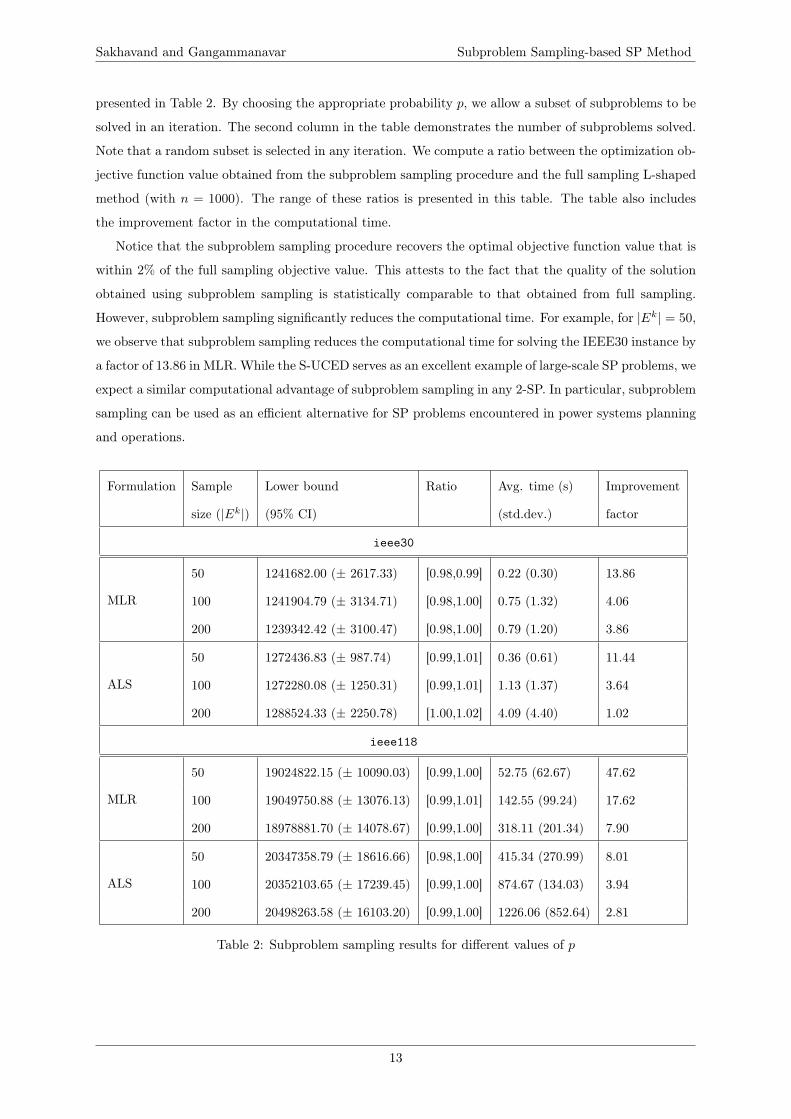
presented in Table 2. By choosing the appropriate probability p, we allow a subset of subproblems to be
solved in an iteration. The second column in the table demonstrates the number of subproblems solved.
Note that a random subset is selected in any iteration. We compute a ratio between the optimization ob-
jective function value obtained from the subproblem sampling procedure and the full sampling L-shaped
method (with n = 1000). The range of these ratios is presented in this table. The table also includes
the improvement factor in the computational time.
Notice that the subproblem sampling procedure recovers the optimal objective function value that is
within 2% of the full sampling objective value. This attests to the fact that the quality of the solution
obtained using subproblem sampling is statistically comparable to that obtained from full sampling.
However, subproblem sampling significantly reduces the computational time. For example, for |Ek| = 50,
we observe that subproblem sampling reduces the computational time for solving the IEEE30 instance by
a factor of 13.86 in MLR. While the S-UCED serves as an excellent example of large-scale SP problems, we
expect a similar computational advantage of subproblem sampling in any 2-SP. In particular, subproblem
sampling can be used as an efficient alternative for SP problems encountered in power systems planning
and operations.
Formulation Sample Lower bound Ratio Avg. time (s) Improvement
size (|Ek|) (95% CI) (std.dev.) factor
ieee30
MLR
50 1241682.00 (± 2617.33) [0.98,0.99] 0.22 (0.30) 13.86
100 1241904.79 (± 3134.71) [0.98,1.00] 0.75 (1.32) 4.06
200 1239342.42 (± 3100.47) [0.98,1.00] 0.79 (1.20) 3.86
ALS
50 1272436.83 (± 987.74) [0.99,1.01] 0.36 (0.61) 11.44
100 1272280.08 (± 1250.31) [0.99,1.01] 1.13 (1.37) 3.64
200 1288524.33 (± 2250.78) [1.00,1.02] 4.09 (4.40) 1.02
ieee118
MLR
50 19024822.15 (± 10090.03) [0.99,1.00] 52.75 (62.67) 47.62
100 19049750.88 (± 13076.13) [0.99,1.01] 142.55 (99.24) 17.62
200 18978881.70 (± 14078.67) [0.99,1.00] 318.11 (201.34) 7.90
ALS
50 20347358.79 (± 18616.66) [0.98,1.00] 415.34 (270.99) 8.01
100 20352103.65 (± 17239.45) [0.99,1.00] 874.67 (134.03) 3.94
200 20498263.58 (± 16103.20) [0.99,1.00] 1226.06 (852.64) 2.81
Table 2: Subproblem sampling results for different values of p
13
Sakhavand and Gangammanavar Subproblem Sampling-based SP Method
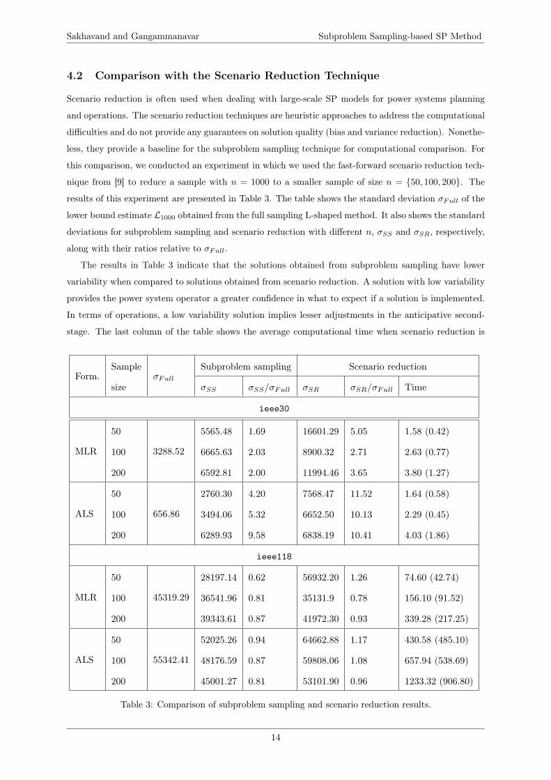
4.2 Comparison with the Scenario Reduction Technique
Scenario reduction is often used when dealing with large-scale SP models for power systems planning
and operations. The scenario reduction techniques are heuristic approaches to address the computational
difficulties and do not provide any guarantees on solution quality (bias and variance reduction). Nonethe-
less, they provide a baseline for the subproblem sampling technique for computational comparison. For
this comparison, we conducted an experiment in which we used the fast-forward scenario reduction tech-
nique from [9] to reduce a sample with n = 1000 to a smaller sample of size n = {50, 100, 200}. The
results of this experiment are presented in Table 3. The table shows the standard deviation σFull of the
lower bound estimate L1000 obtained from the full sampling L-shaped method. It also shows the standard
deviations for subproblem sampling and scenario reduction with different n, σSS and σSR, respectively,
along with their ratios relative to σFull.
The results in Table 3 indicate that the solutions obtained from subproblem sampling have lower
variability when compared to solutions obtained from scenario reduction. A solution with low variability
provides the power system operator a greater confidence in what to expect if a solution is implemented.
In terms of operations, a low variability solution implies lesser adjustments in the anticipative second-
stage. The last column of the table shows the average computational time when scenario reduction is
Form.Sample
σFullSubproblem sampling Scenario reduction
size σSS σSS/σFull σSR σSR/σFull Time
ieee30
MLR
50
3288.52
5565.48 1.69 16601.29 5.05 1.58 (0.42)
100 6665.63 2.03 8900.32 2.71 2.63 (0.77)
200 6592.81 2.00 11994.46 3.65 3.80 (1.27)
ALS
50
656.86
2760.30 4.20 7568.47 11.52 1.64 (0.58)
100 3494.06 5.32 6652.50 10.13 2.29 (0.45)
200 6289.93 9.58 6838.19 10.41 4.03 (1.86)
ieee118
MLR
50
45319.29
28197.14 0.62 56932.20 1.26 74.60 (42.74)
100 36541.96 0.81 35131.9 0.78 156.10 (91.52)
200 39343.61 0.87 41972.30 0.93 339.28 (217.25)
ALS
50
55342.41
52025.26 0.94 64662.88 1.17 430.58 (485.10)
100 48176.59 0.87 59808.06 1.08 657.94 (538.69)
200 45001.27 0.81 53101.90 0.96 1233.32 (906.80)
Table 3: Comparison of subproblem sampling and scenario reduction results.
14
Sakhavand and Gangammanavar Subproblem Sampling-based SP Method
employed. This time includes the time of executing the fast-forward technique as well as optimization
using the L-shaped method. Notice that the average time taking by subproblem sampling (see Table 2)
is lower in all but one instance. Therefore, subproblem sampling not only provides a solution with low
variability but also does so in computationally less time.
4.3 Identifying a Solution for Prescription
Since the SAA is constructed using a sample Ξn that is generated at random, the optimal objective
function value v∗n as well as the optimal solution (x∗n, z∗n), are random functions of Ξn. Performing a
single replication results in a single realization of these random functions. Moreover, the SAA theory
suggests that the SAA optimal value is biased downwards, i.e., E[v∗n] ≤ v∗ (see [26]). Therefore, the
SAA optimal value underestimates (in expectation) the true optimal value. In order to assess the extent
of the bias and the quality of the solution, performing the replicated experiments as presented in §3.2 is
an essential step. Note that the replications can be carried out in parallel as they involve independent
optimization and out-of-sample assessment steps.
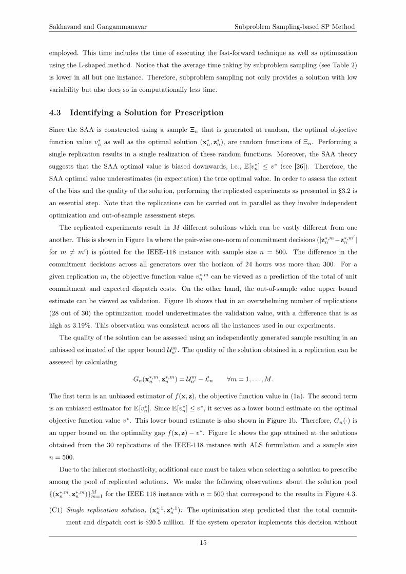
The replicated experiments result in M different solutions which can be vastly different from one
another. This is shown in Figure 1a where the pair-wise one-norm of commitment decisions (|z∗,mn −z∗,m′
n |
for m 6= m′) is plotted for the IEEE-118 instance with sample size n = 500. The difference in the
commitment decisions across all generators over the horizon of 24 hours was more than 300. For a
given replication m, the objective function value v∗,mn can be viewed as a prediction of the total of unit
commitment and expected dispatch costs. On the other hand, the out-of-sample value upper bound
estimate can be viewed as validation. Figure 1b shows that in an overwhelming number of replications
(28 out of 30) the optimization model underestimates the validation value, with a difference that is as
high as 3.19%. This observation was consistent across all the instances used in our experiments.
The quality of the solution can be assessed using an independently generated sample resulting in an
unbiased estimated of the upper bound Umn′ . The quality of the solution obtained in a replication can be
assessed by calculating
Gn(x∗,mn , z∗,mn ) = Umn′ − Ln ∀m = 1, . . . ,M.
The first term is an unbiased estimator of f(x, z), the objective function value in (1a). The second term
is an unbiased estimator for E[v∗n]. Since E[v∗n] ≤ v∗, it serves as a lower bound estimate on the optimal
objective function value v∗. This lower bound estimate is also shown in Figure 1b. Therefore, Gn(·) is
an upper bound on the optimality gap f(x, z) − v∗. Figure 1c shows the gap attained at the solutions
obtained from the 30 replications of the IEEE-118 instance with ALS formulation and a sample size
n = 500.
Due to the inherent stochasticity, additional care must be taken when selecting a solution to prescribe
among the pool of replicated solutions. We make the following observations about the solution pool
{(x∗,mn , z∗,mn )}Mm=1 for the IEEE 118 instance with n = 500 that correspond to the results in Figure 4.3.
(C1) Single replication solution, (x∗,1n , z∗,1n ): The optimization step predicted that the total commit-
ment and dispatch cost is $20.5 million. If the system operator implements this decision without
15
Sakhavand and Gangammanavar Subproblem Sampling-based SP Method
(a) One-norm difference between solutions
0 5 10 15 20 25 30
Replications
2.02
2.04
2.06
2.08
2.1
2.1210
7
Prediction
Validation
LB Estimate
(b) Lower and upper bound estimates
0 5 10 15 20 25 30
Replications
-1
0
1
2
3
4
Op
tim
alit
y g
ap
(%
)
(c) Out-of-sample gap
Figure 1: Results for IEEE-118 ALS instance with n = 500.
validation, then the system operator will incur a cost that is higher by as much as 1.6%.
(C2) Solution with the smallest lower bound estimate: After completing M replications, select µ such
that v∗n,µ ≤ v∗n,m for all m = 1, . . . ,M . The solution (x∗,µn , z∗,µn ) corresponds to the one with
the smallest lower bound. For the instance under consideration µ = 13. If the system operator
implements this solution, the total commitment and expected dispatch cost will be $20.32 million.
However, the validation results show that the total costs can be higher by at most 1.35% at $20.59
16
Sakhavand and Gangammanavar Subproblem Sampling-based SP Method
million.
(C3) Solution with the smallest upper bound estimate: After completing the optimization and evaluation
steps, identify the replication that yields a solution with the smallest upper bound. That is, select
µ such that Uµn′ ≤ Umn′ for all m = 1, . . . ,M . For the instance under study, the replication identified
using the smallest upper bound criterion is µ = 28 with a validation value of $20.37 million.
(C4) Solution with the smallest optimality gap: Identify the replication index as
µ ∈ argminm=1,...,M
{Gn(x∗,mn , z∗,mn )
}.
For the instance under consideration, µ = 28. The solution identified using this criterion results in
a validation value ($20.37 million) that is lower than the prediction value ($20.40 million).
For selecting an appropriate solution for prescription, the above criteria must be used in the reverse
order. That is, the solution with the smallest out-of-sample gap estimate receives, that is criterion
(C4), the highest preference for prescription. However, for large-scale S-UCED problems that cannot
be solved to optimality, the solution with the smallest out-of-sample is not guaranteed to provide the
smallest optimality gap. This is the case with the IEEE-118 instances as indicated by the large instance
optimization gap column in Table 1. The criterion (C4) is applicable for IEEE-30 instances. For the
IEEE-118 instance, a solution identified using (C3) is appropriate for prescription.
4.4 Comparison of Results from MLR and ALS Formulations.
We conclude our discussion on numerical results by comparing the solutions and the value associated with
the MLR and ALS formulations of the S-UCED. Recall that in the MLR formulation, a separate variable
is used to capture the capability of the generator to provide the spinning reserve. On the other hand,
the ALS formulation models the maximum generation after adjusting for uncertainty. This maximum
generation implicitly captures the reserve capability of the generator. This difference between the two
formulations has a significant impact on the overall operating cost.
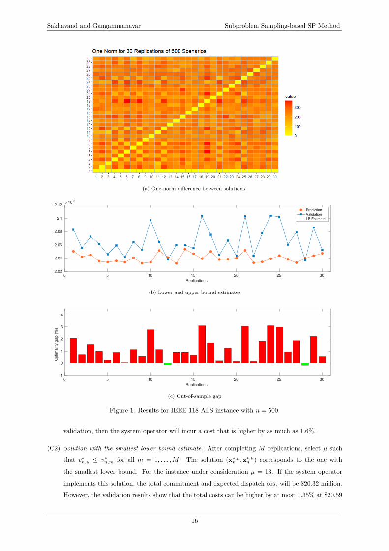
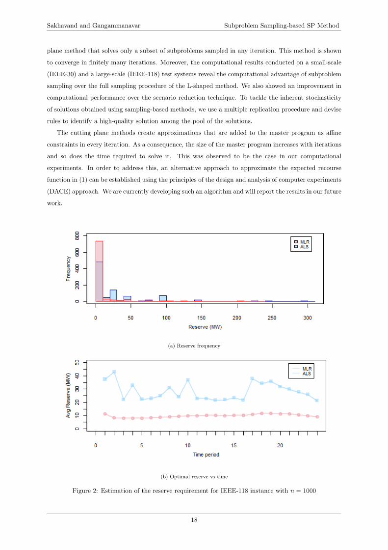
The results in Tables 1, 2 and 3 show that the overall cost corresponding to the ALS formulation
is higher when compared to the cost associated with MLR formulation. This can be attributed to a
higher amount of reserve requirement estimated by the ALS formulation. This can be seen in Figure
2. The histogram in Figure 2a shows the number of the generators providing a certain level of reserve
capability and Figure 2b illustrates the average per generator over 24-hour horizon. In this sense, the
ALS formulation is more conservative when compared to the MLR formulation. The ALS formulation
is also computationally more expensive in comparison.
5 Conclusion
In this paper, we presented a stochastic optimization and simulation framework which utilizes two for-
mulations of S-UCED with uncertainties in renewable generation. The resulting formulations are 2-SLPs
with mixed-binary first-stage decisions and continuous recourse. We presented a sampling-based cutting
17
Sakhavand and Gangammanavar Subproblem Sampling-based SP Method
plane method that solves only a subset of subproblems sampled in any iteration. This method is shown
to converge in finitely many iterations. Moreover, the computational results conducted on a small-scale
(IEEE-30) and a large-scale (IEEE-118) test systems reveal the computational advantage of subproblem
sampling over the full sampling procedure of the L-shaped method. We also showed an improvement in
computational performance over the scenario reduction technique. To tackle the inherent stochasticity
of solutions obtained using sampling-based methods, we use a multiple replication procedure and devise
rules to identify a high-quality solution among the pool of the solutions.
The cutting plane methods create approximations that are added to the master program as affine
constraints in every iteration. As a consequence, the size of the master program increases with iterations
and so does the time required to solve it. This was observed to be the case in our computational
experiments. In order to address this, an alternative approach to approximate the expected recourse
function in (1) can be established using the principles of the design and analysis of computer experiments
(DACE) approach. We are currently developing such an algorithm and will report the results in our future
work.
(a) Reserve frequency
(b) Optimal reserve vs time
Figure 2: Estimation of the reserve requirement for IEEE-118 instance with n = 1000
18
Sakhavand and Gangammanavar Subproblem Sampling-based SP Method
The subproblem sampling procedure works with a SAA of the the (1) that uses a finite number of
observations. In our numerical study, each time the number of observations is increased, the optimization
algorithm is restarted from scratch. Completing such an approach in a time-sensitive settings of power
systems operations may prove to be challenging without high-performance computing resources. The
sequential sampling algorithms, particularly the stochastic decomposition (SD) method [10], have proven
to be effective in addressing this computational challenge. The current SD method does not support
binary variables in the first-stage. We will undertake the development of the SD method customized to
the S-UCED in our future research endeavor.
A Nomenclature
Sets
T Time scale decision epochs
B Buses
L Transmission lines
D Demand
G Conventional generators
R Renewable generators
Generator Parameters
Cg/Cg Minimum/maximum required generatio when g is operational
Rg/Rg Ramp-up/ ramp-down limit at generator g
Sg/Sg Start-up/ shut down limit at generator g
UTg/DTg Minimum uptime/ downtime limit at generator g
fSUg,t /fSDg,t Incurred startup/shutdown cost for generator g at time t
c0g No-load cost at generator g
cκg Variable cost of the κth piece for generator g
dgsg Shedding penalty at generator g
γκg Production amount of the κth piece at generator g, κ = {1, .., κmax}
V (γκg ) Aggregated cost of generating γκg units of output
19
Sakhavand and Gangammanavar Subproblem Sampling-based SP Method
Bus and Line Parameters
V Bus voltage
θmin, θmax Angle limits of the connected buses
pmin, pmax Line capacity limits
X Line reactance
Other Parameters
Di,t Demand at demand node i at time t
ρt The required reserve amount at time t
dlsi Value of lost load at demand node i
Gg,t Total amount of available renewable energy at
the renewable generator g at time t
UC MLR Decision Variables
xg,t 1 if g is online at period t, 0 otherwise
sg,t/zg,t 1 if g is turned on/off, 0 otherwise
G′g,t Day-ahead production amount beyond Cg provided by generator g at time t
rg,t Spinning reserve provided by unit g at time t
UC ALS Decision Variables
xg,t 1 if g remains operational at period t, 0 otherwise
sg,t/zg,t 1 if g is turned on/off, 0 otherwise
G′g,t Day-ahead production amount beyond Cg provided by generator g at time t
Gg,t Maximum day-ahead generation amount that g can supply at time t
20
Sakhavand and Gangammanavar Subproblem Sampling-based SP Method
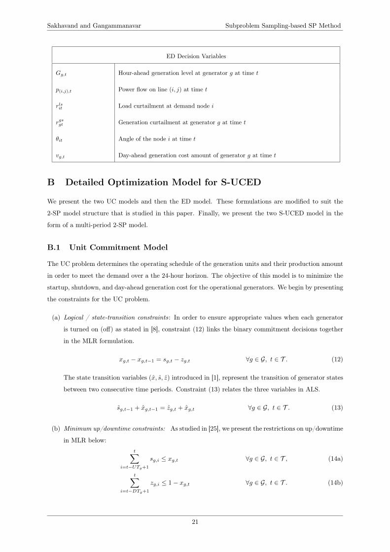
ED Decision Variables
Gg,t Hour-ahead generation level at generator g at time t
p(i,j),t Power flow on line (i, j) at time t
rlsit Load curtailment at demand node i
rgsgt Generation curtailment at generator g at time t
θit Angle of the node i at time t
vg,t Day-ahead generation cost amount of generator g at time t
B Detailed Optimization Model for S-UCED
We present the two UC models and then the ED model. These formulations are modified to suit the
2-SP model structure that is studied in this paper. Finally, we present the two S-UCED model in the
form of a multi-period 2-SP model.
B.1 Unit Commitment Model
The UC problem determines the operating schedule of the generation units and their production amount
in order to meet the demand over a the 24-hour horizon. The objective of this model is to minimize the
startup, shutdown, and day-ahead generation cost for the operational generators. We begin by presenting
the constraints for the UC problem.
(a) Logical / state-transition constraints: In order to ensure appropriate values when each generator
is turned on (off) as stated in [8], constraint (12) links the binary commitment decisions together
in the MLR formulation.
xg,t − xg,t−1 = sg,t − zg,t ∀g ∈ G, t ∈ T . (12)
The state transition variables (x, s, z) introduced in [1], represent the transition of generator states
between two consecutive time periods. Constraint (13) relates the three variables in ALS.
sg,t−1 + xg,t−1 = zg,t + xg,t ∀g ∈ G, t ∈ T . (13)
(b) Minimum up/downtime constraints: As studied in [25], we present the restrictions on up/downtime
in MLR below:t∑
i=t−UTg+1
sg,i ≤ xg,t ∀g ∈ G, t ∈ T , (14a)
t∑i=t−DTg+1
zg,i ≤ 1− xg,t ∀g ∈ G, t ∈ T . (14b)
21
Sakhavand and Gangammanavar Subproblem Sampling-based SP Method
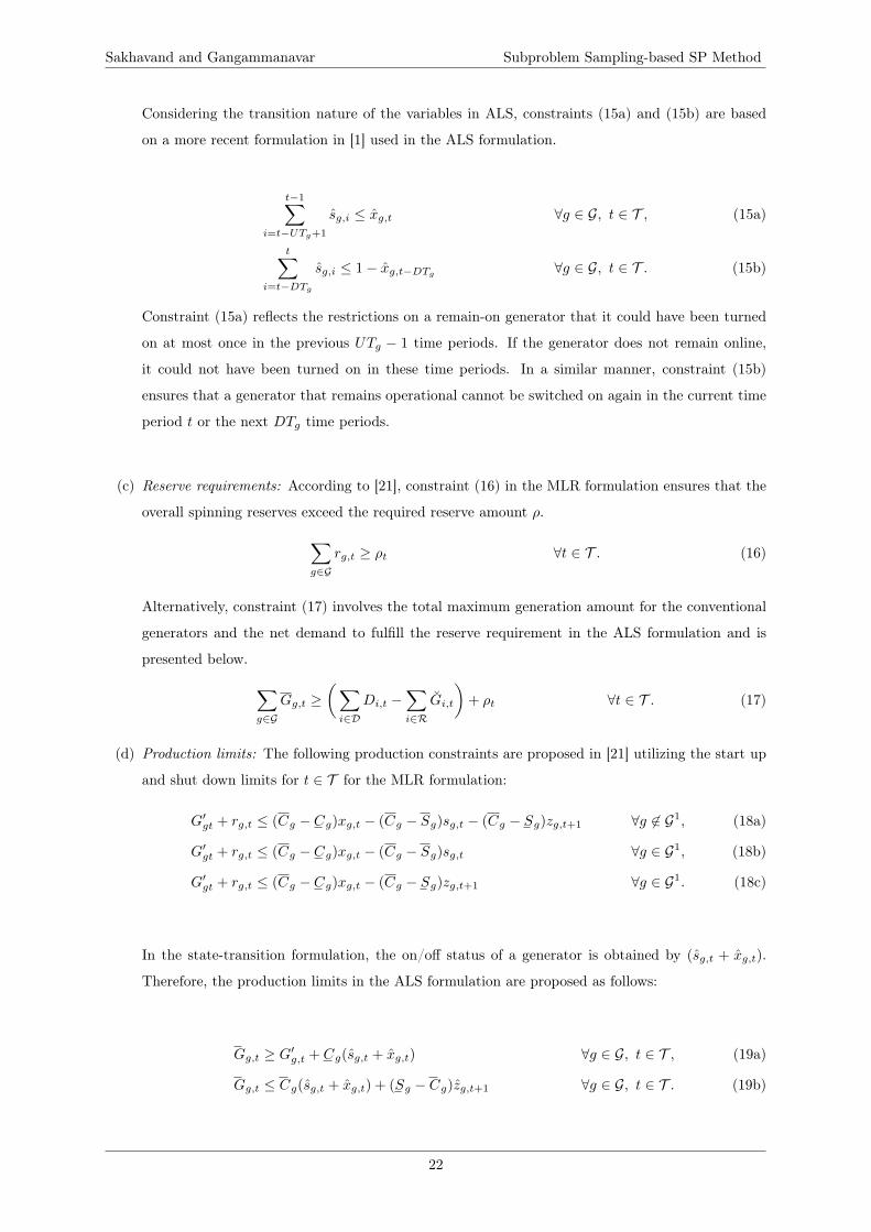
Considering the transition nature of the variables in ALS, constraints (15a) and (15b) are based
on a more recent formulation in [1] used in the ALS formulation.
t−1∑i=t−UTg+1
sg,i ≤ xg,t ∀g ∈ G, t ∈ T , (15a)
t∑i=t−DTg
sg,i ≤ 1− xg,t−DTg∀g ∈ G, t ∈ T . (15b)
Constraint (15a) reflects the restrictions on a remain-on generator that it could have been turned
on at most once in the previous UTg − 1 time periods. If the generator does not remain online,
it could not have been turned on in these time periods. In a similar manner, constraint (15b)
ensures that a generator that remains operational cannot be switched on again in the current time
period t or the next DTg time periods.
(c) Reserve requirements: According to [21], constraint (16) in the MLR formulation ensures that the
overall spinning reserves exceed the required reserve amount ρ.∑g∈G
rg,t ≥ ρt ∀t ∈ T . (16)
Alternatively, constraint (17) involves the total maximum generation amount for the conventional
generators and the net demand to fulfill the reserve requirement in the ALS formulation and is
presented below. ∑g∈G
Gg,t ≥(∑i∈D
Di,t −∑i∈R
Gi,t
)+ ρt ∀t ∈ T . (17)
(d) Production limits: The following production constraints are proposed in [21] utilizing the start up
and shut down limits for t ∈ T for the MLR formulation:
G′gt + rg,t ≤ (Cg − Cg)xg,t − (Cg − Sg)sg,t − (Cg − Sg)zg,t+1 ∀g 6∈ G1, (18a)
G′gt + rg,t ≤ (Cg − Cg)xg,t − (Cg − Sg)sg,t ∀g ∈ G1, (18b)
G′gt + rg,t ≤ (Cg − Cg)xg,t − (Cg − Sg)zg,t+1 ∀g ∈ G1. (18c)
In the state-transition formulation, the on/off status of a generator is obtained by (sg,t + xg,t).
Therefore, the production limits in the ALS formulation are proposed as follows:
Gg,t ≥ G′g,t + Cg(sg,t + xg,t) ∀g ∈ G, t ∈ T , (19a)
Gg,t ≤ Cg(sg,t + xg,t) + (Sg − Cg)zg,t+1 ∀g ∈ G, t ∈ T . (19b)
22
Sakhavand and Gangammanavar Subproblem Sampling-based SP Method
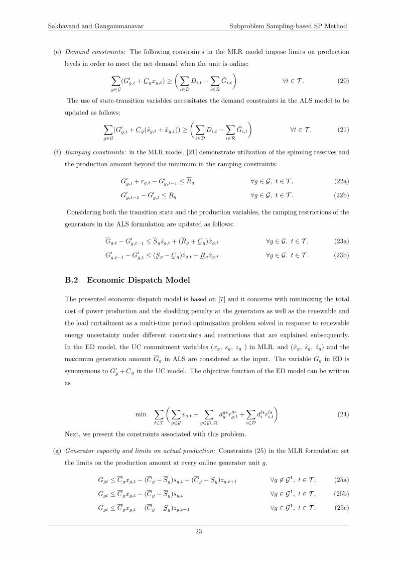
(e) Demand constraints: The following constraints in the MLR model impose limits on production
levels in order to meet the net demand when the unit is online:∑g∈G
(G′g,t + Cgxg,t) ≥(∑i∈D
Di,t −∑i∈R
Gi,t
)∀t ∈ T . (20)
The use of state-transition variables necessitates the demand constraints in the ALS model to be
updated as follows:∑g∈G
(G′g,t + Cg(sg,t + xg,t)) ≥(∑i∈D
Di,t −∑i∈R
Gi,t
)∀t ∈ T . (21)
(f) Ramping constraints: in the MLR model, [21] demonstrate utilization of the spinning reserves and
the production amount beyond the minimum in the ramping constraints:
G′g,t + rg,t −G′g,t−1 ≤ Rg ∀g ∈ G, t ∈ T , (22a)
G′g,t−1 −G′g,t ≤ Rg ∀g ∈ G, t ∈ T . (22b)
Considering both the transition state and the production variables, the ramping restrictions of the
generators in the ALS formulation are updated as follows:
Gg,t −G′g,t−1 ≤ Sg sg,t + (Rg + Cg)xg,t ∀g ∈ G, t ∈ T , (23a)
G′g,t−1 −G′g,t ≤ (Sg − Cg)zg,t +Rgxg,t ∀g ∈ G, t ∈ T . (23b)
B.2 Economic Dispatch Model
The presented economic dispatch model is based on [7] and it concerns with minimizing the total
cost of power production and the shedding penalty at the generators as well as the renewable and
the load curtailment as a multi-time period optimization problem solved in response to renewable
energy uncertainty under different constraints and restrictions that are explained subsequently.
In the ED model, the UC commitment variables (xg, sg, zg ) in MLR, and (xg, sg, zg) and the
maximum generation amount Gg in ALS are considered as the input. The variable Gg in ED is
synonymous to G′g +Cg in the UC model. The objective function of the ED model can be written
as
min∑t∈T
(∑g∈G
vg,t +∑
g∈G∪Rdgsg r
gsg,t +
∑i∈D
dlsi rlsi,t
)(24)
Next, we present the constraints associated with this problem.
(g) Generator capacity and limits on actual production: Constraints (25) in the MLR formulation set
the limits on the production amount at every online generator unit g.
Ggt ≤ Cgxg,t − (Cg − Sg)sg,t − (Cg − Sg)zg,t+1 ∀g 6∈ G1, t ∈ T , (25a)
Ggt ≤ Cgxg,t − (Cg − Sg)sg,t ∀g ∈ G1, t ∈ T , (25b)
Ggt ≤ Cgxg,t − (Cg − Sg)zg,t+1 ∀g ∈ G1, t ∈ T . (25c)
23
Sakhavand and Gangammanavar Subproblem Sampling-based SP Method
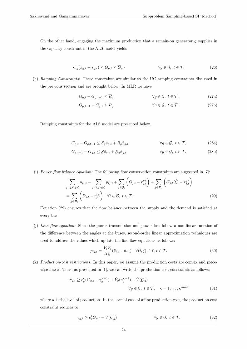
On the other hand, engaging the maximum production that a remain-on generator g supplies in
the capacity constraint in the ALS model yields
Cg(xg,t + sg,t) ≤ Gg,t ≤ Gg,t ∀g ∈ G, t ∈ T . (26)
(h) Ramping Constraints: These constraints are similar to the UC ramping constraints discussed in
the previous section and are brought below. In MLR we have
Gg,t −Gg,t−1 ≤ Rg ∀g ∈ G, t ∈ T , (27a)
Gg,t−1 −Gg,t ≤ Rg ∀g ∈ G, t ∈ T . (27b)
Ramping constraints for the ALS model are presented below.
Gg,t −Gg,t−1 ≤ Sg sg,t +Rgxg,t ∀g ∈ G, t ∈ T , (28a)
Gg,t−1 −Gg,t ≤ Szg,t +Rgxg,t ∀g ∈ G, t ∈ T . (28b)
(i) Power flow balance equation: The following flow conservation constraints are suggested in [7]:∑j:(j,i)∈L
pji,t −∑
j:(i,j)∈L
pij,t +∑j∈Gi
(Gj,t − rgsj,t
)+∑j∈Ri
(Gj,t(ξ)− rgsj,t
)
=∑j∈Di
(Dj,t − rlsj,t
)∀i ∈ B, t ∈ T . (29)
Equation (29) ensures that the flow balance between the supply and the demand is satisfied at
every bus.
(j) Line flow equation: Since the power transmission and power loss follow a non-linear function of
the difference between the angles at the buses, second-order linear approximation techniques are
used to address the values which update the line flow equations as follows:
pij,t =ViVjXij
(θi,t − θj,t) ∀(i, j) ∈ L, t ∈ T . (30)
(k) Production-cost restrictions: In this paper, we assume the production costs are convex and piece-
wise linear. Thus, as presented in [1], we can write the production cost constraints as follows:
vg,t ≥ cκg (Gg,t − γκ−1g ) + Vg(γκ−1g )− V (Cg)
∀g ∈ G, t ∈ T , κ = 1, . . . , κmax (31)
where κ is the level of production. In the special case of affine production cost, the production cost
constraint reduces to
vg,t ≥ c1gGg,t − V (Cg) ∀g ∈ G, t ∈ T . (32)
24
Sakhavand and Gangammanavar Subproblem Sampling-based SP Method
(l) Bounds: Constraints (33a) and (33b) are the limit on the line capacities and the bus angles
respectively. Additionally, restrictions on the generation and load curtailment variables are given
in (33c) and (33d).
pminij ≤ pij,t ≤ pmaxij ∀(i, j) ∈ L, t ∈ T , (33a)
θmini ≤ θi,t ≤ θmaxi ∀i ∈ B, t ∈ T , (33b)
0 ≤ rlsi,t ≤ Di,t ∀i ∈ D, t ∈ T , (33c)
0 ≤ rgsi,t ≤ Gi,t ∀i ∈ G ∪R, t ∈ T . (33d)
B.3 Decomposed multi period two-stage S-UCED model
The complete formulation of the decomposed multi period two-stage S-UCED models are presented
below. The MLR formulation for the model can be written as
min∑t∈T
(∑g∈G
(fSUg,t sg,t + fSDg,t zg,t + V (Cg)xg,t
))+ E{Q(x, s, z, ξ)} (UC MLR)
s.t (12), (14), (16), (18), (20), (22)
(x, s, z, ) ∈ {0, 1}3|G||T |, (G′, r) ≥ 0
where,
Q(x, s, z, ξ) = min∑t∈T
(∑g∈G
vg,t +∑
g∈G∪Rdgsg r
gsg,t +
∑i∈D
dlsi rlsi,t
)(ED MLR)
s.t (25), (27), (29), (30), (32), (33), (G, v) ≥ 0.
Second, the ALS formulation is presented.
min∑t∈T
(∑g∈G
(fSUg,t sg,t + fSDg,t zg,t + V (Cg)(sg,t + xg,t)
))+ E{Q(x, s, z, G, ξ)} (UC ALS)
s.t (13), (15), (17), (19), (21), (23)
(x, s, z) ∈ {0, 1}3|G||T |, (G′, G) ≥ 0
where,
Q(x, s, z, G, ξ) = min∑t∈T
(∑g∈G
vg,t +∑
g∈G∪Rdgsg r
gsg,t +
∑i∈D
dlsi rlsi,t
)(ED ALS)
s.t (26), (28)− (30), (32), (33), (G, v) ≥ 0.
References
[1] Semih Atakan, Guglielmo Lulli, and Suvrajeet Sen. A state transition mip formulation for the unit
commitment problem. IEEE Transactions on Power Systems, 33(1):736–748, 2017.
25
Sakhavand and Gangammanavar Subproblem Sampling-based SP Method
[2] Francois Bouffard and Francisco D Galiana. Stochastic security for operations planning with signifi-
cant wind power generation. In 2008 IEEE Power and Energy Society General Meeting-Conversion
and Delivery of Electrical Energy in the 21st Century, pages 1–11. IEEE, 2008.
[3] Miguel Carrión and José M Arroyo. A computationally efficient mixed-integer linear formulation
for the thermal unit commitment problem. IEEE Transactions on power systems, 21(3):1371–1378,
2006.
[4] J. Dupačová, N. Gröwe-Kuska, and W. Römisch. Scenario reduction in stochastic programming.
Mathematical Programming, 95(3):493–511, 2003.
[5] Yonghan Feng and Sarah M. Ryan. Solution sensitivity-based scenario reduction for stochastic unit
commitment. Computational Management Science, 13:29–62, 2016.
[6] Harsha Gangammanavar, Yifan Liu, and Suvrajeet Sen. Stochastic decomposition for two-stage
stochastic linear programs with random cost coefficients. INFORMS Journal on Computing, 2020.
[7] Harsha Gangammanavar, Suvrajeet Sen, and Victor M Zavala. Stochastic optimization of sub-
hourly economic dispatch with wind energy. IEEE Transactions on Power Systems, 31(2):949–959,
2015.
[8] Len L Garver. Power generation scheduling by integer programming-development of theory. Trans-
actions of the American Institute of Electrical Engineers. Part III: Power Apparatus and Systems,
81(3):730–734, 1962.
[9] H. Heitsch and W. Romisch. Scenario reduction algorithms in stochastic programming. Computa-
tional Optimization and Applications, 24(2-3):187–206, 2003.
[10] J. L. Higle and S Sen. Stochastic decomposition: An algorithm for two-stage linear programs with
recourse. Mathematics of Operations Research, 16(3):650–669, 1991.
[11] J. L. Higle and S Sen. Stochastic Decomposition: A Statistical Method for Large Scale Stochastic
Linear Programming. Kluwer Academic Publishers, Boston, MA., 1996.
[12] Kjetil Høyland, Michal Kaut, and Stein W Wallace. A heuristic for moment-matching scenario
generation. Computational optimization and applications, 24(2-3):169–185, 2003.
[13] Anton J Kleywegt, Alexander Shapiro, and Tito Homem-de Mello. The sample average approxima-
tion method for stochastic discrete optimization. SIAM Journal on Optimization, 12(2):479–502,
2002.
[14] Sam Koebrich, Thomas Bowen, and Austen Sharpe. 2018 Renewable Energy Data Book, 2018.
[15] J. Linderoth, A. Shapiro, and S. Wright. The empirical behavior of sampling methods for stochastic
programming. Annals of Operations Research, 142(1):215–241, 2006.
26
Sakhavand and Gangammanavar Subproblem Sampling-based SP Method
[16] K Liu and J Zhong. Generation dispatch considering wind energy and system reliability. In IEEE
PES General Meeting, pages 1–7, 2010.
[17] Yang Liu and Nirmal-Kumar C Nair. A two-stage stochastic dynamic economic dispatch model
considering wind uncertainty. IEEE Transactions on Sustainable Energy, 7(2):819–829, 2015.
[18] Wai-Kei Mak, David P Morton, and R Kevin Wood. Monte carlo bounding techniques for deter-
mining solution quality in stochastic programs. Operations research letters, 24(1-2):47–56, 1999.
[19] J. M. Morales, A. J. Conejo, and J. Perez-Ruiz. Economic valuation of reserves in power systems
with high penetration of wind power. IEEE Transactions on Power Systems, 24(2):900–910, 2009.
[20] J. M. Morales, S. Pineda, A. J. Conejo, and M. Carrion. Scenario reduction for futures market
trading in electricity markets. IEEE Transactions on Power Systems, 24(2):878–888, 2009.
[21] Germán Morales-España, Jesus M Latorre, and Andres Ramos. Tight and compact milp formulation
for the thermal unit commitment problem. IEEE Transactions on Power Systems, 28(4):4897–4908,
2013.
[22] GJ Osório, JM Lujano-Rojas, JCO Matias, and JPS Catalão. A probabilistic approach to solve the
economic dispatch problem with intermittent renewable energy sources. Energy, 82:949–959, 2015.
[23] A Papavasiliou and S.S. Oren. Multiarea stochastic unit commitment for high wind penetration in
a transmission constrained network. Operations Research, 61(3):578–592, 2013.
[24] A Papavasiliou, S.S. Oren, and R.P. O’Neill. Reserve requirements for wind power integration:
A scenario-based stochastic programming framework. IEEE Transactions on Power Systems,
26(4):2197–2206, Nov 2011.
[25] Deepak Rajan, Samer Takriti, et al. Minimum up/down polytopes of the unit commitment problem
with start-up costs. IBM Res. Rep, 23628:1–14, 2005.
[26] A. Shapiro, D. Dentcheva, and A. Ruszczynski. Lectures on Stochastic Programming: Modeling and
Theory, Second Edition. Society for Industrial and Applied Mathematics, Philadelphia, PA, USA,
2014.
[27] U.S. Energy Information Administration. Annual Energy Outlook 2020 with projections to 2050,
2020.
[28] Richard M Van Slyke and Roger Wets. L-shaped linear programs with applications to optimal
control and stochastic programming. SIAM Journal on Applied Mathematics, 17(4):638–663, 1969.
[29] Jiadong Wang, Jianhui Wang, Cong Liu, and Juan P Ruiz. Stochastic unit commitment with
sub-hourly dispatch constraints. Applied energy, 105:418–422, 2013.
[30] Jianhui Wang, Audun Botterud, Vladimiro Miranda, Cláudio Monteiro, and Gerald Sheble. Impact
of wind power forecasting on unit commitment and dispatch. In Proc. 8th Int. Workshop Large-Scale
Integration of Wind Power into Power Systems, pages 1–8, 2009.
27

Sakhavand and Gangammanavar Subproblem Sampling-based SP Method
[31] Rolf Wiebking. Stochastische modelle zur optimalen lastverteilung in einem kraftwerksverbund.
Zeitschrift für Operations Research, 21(6):B197–B217, 1977.
[32] Lei Wu, Mohammad Shahidehpour, and Tao Li. Stochastic security-constrained unit commitment.
IEEE Transactions on power systems, 22(2):800–811, 2007.
[33] Bining Zhao, Antonio J Conejo, and Ramteen Sioshansi. Unit commitment under gas-supply un-
certainty and gas-price variability. IEEE Transactions on Power Systems, 32(3):2394–2405, 2016.
[34] Qipeng P Zheng, Jianhui Wang, and Andrew L Liu. Stochastic optimization for unit commitment—a
review. IEEE Transactions on Power Systems, 30(4):1913–1924, 2014.
28