Embed Size (px)
Citation preview
Subseasonal variations of tropical convection and week two
prediction of wintertime western North American rainfall
Jeffrey S. Whitaker and Klaus M. Weickmann
NOAA-CIRES Climate Diagnostics Center, Boulder, Colorado
Manuscript to appear in J. Climate
Submitted to Journal of Climate

1
Corresponding author address: Jeffrey S. Whitaker, NOAA-CIRES Climate
Diagnostics Center, 325 Broadway, Boulde-3328. [email protected]

2
Abstract
A statistical prediction model for weekly rainfall during winter over western North
America is developed which uses tropical outgoing longwave radiation (OLR) anomalies
as a predictor. The effects of El Nino-Southern Oscillation (ENSO) are linearly removed
from the OLR to isolate the predictive utility of subseasonal variations in tropical
convection. A single canonical correlation (CCA) mode accounts for most of the
predictable signal. The rank correlation between this mode and observed rainfall
anomalies over Southern California is 0.2 for a two-week lag, which is comparable to
correlation between a weekly ENSO index and weekly rainfall in this region. This
corresponds to a doubling of the risk of extreme rainfall in Southern California when the
projection of tropical OLR on the leading CCA mode two weeks prior is extremely large,
compared to times when it is extremely small. ‘Extreme’ is defined as being in the upper
or lower quintile of the probability distribution.
The leading CCA mode represents suppressed convection in the equatorial Indian
Ocean and enhanced convection just south of the equator east of the dateline. OLR
regressed on the time series of this mode show an eastward progression of the suppressed
region to just south of the Philippines at the time of maximum California rainfall
enhancement. The region of enhanced convection east of the dateline remains quasi-
stationary. Associated with this tropical OLR evolution is the development of upper
tropospheric westerly wind anomalies near 30oN in the eastern Pacific. Synoptic-scale
weather systems are steered farther east toward California by these enhanced westerlies.

3
Since most operational weather prediction models do not accurately simulate
subseasonal variations in tropical convection, statistical prediction models such as the one
presented here may prove useful in augmenting numerical predictions. An analysis of four
years of operational week two ensemble predictions indicates that the level of skill
provided by the statistical model is comparable to that of the operational ensemble mean.
Since by week two the operational forecast model has lost its ability to represent
convectively coupled circulation associated with the subseasonal tropical convective
variability, the statistical model provides essentially independent information for the
forecaster.
4
1. Introduction.
Variations of tropical convection on subseasonal time-scales are known to affect
the distribution of precipitation over western North America in wintertime (Mo and
Higgins 1998a,b, Jones 2000). However, many, if not all, current operational weather
prediction models are unable to predict subseasonal variations of tropical convection,
particularly those associated with the Madden-Julian oscillation (MJO), at ranges beyond a
few days (Hendon at al, 2000). In fact, current data assimilation systems do not even
capture aspects of the MJO very well, most likely because it occurs in a region of sparse
observations where the analysis is heavily influenced by the assimilating model (Newman
et al 2000). This suggests that precipitation forecasts over North America could be
improved, particularly in the medium and extended range, by improving predictions of
subseasonal variations in tropical convection.
Waliser et al (1999) developed a statistical model to predict tropical rainfall
variability at lead times of 5-20 days and found that the statistical model performed
considerably better than global numerical forecasts from the National Centers for
Environmental Prediction (NCEP). However, since their model used bandpass filtered
OLR as a predictor, it cannot easily be used to make real-time predictions. In this study,
we will present a statistical prediction model utilizing the latest 7-day average tropical
OLR field to predict rainfall over western North America directly two weeks later. The
model has been designed to be used as a real-time forecast model, and to isolate the
predictability of western North American rainfall associated with subseasonal tropical
convective variability. Since the value of El Nino/Southern Oscillation (ENSO) in

5
predicting seasonal mean rainfall in this region has already been well established (Schonher
and Nicholson 1989, Barnston et al 1999), we chose to focus on the predictability
associated with subseasonal OLR variability by linearly removing the ENSO signal from
the weekly OLR data. The predictive skill obtained by using subseasonal OLR as a
predictor is compared with week two rainfall predictions produced by the NCEP
operational ensemble prediction system (Toth and Kalnay 1993) and the predictability of
weekly rainfall associated with ENSO. Since our model is linear, and only takes into
account the initial distribution of tropical OLR, it can be considered a lower bound on the
potential for increasing forecast skill by improving the representation of subseasonal
tropical convective variability in operational prediction systems.
2. Data and Analysis Procedure.
The 2.5o gridded daily OLR dataset described by Liebmann and Smith (1996) is
used as a proxy for tropical convection. Data for 25 winter seasons is used, from
December – February (DJF) 1974/1975 to 1999/2000. DJF 1978/1979 is excluded, since
much of the data is missing due to instrument problems. The data is smoothed to
emphasize large-scale features using a Gaussian spectral filter (Sardeshmukh and Hoskins
1984) of the form exp(-(n/20)2), where n is the total wavenumber in spherical harmonic
space. This is roughly equivalent to averaging the OLR over a circular region with a
radius of about 800 km. After the spatial smoothing, the OLR data is interpolated to a 5o
grid and then temporally smoothed by applying a seven-day running average. The linear
ENSO signal in OLR is defined by linearly regressing the spatially smoothed, weekly OLR

6
data on to the first two principal components (PCs) of 7-day averaged sea surface
temperature from the NCEP/NCAR reanalysis (Kalnay et al, 1996)1. This linear signal is
removed from the data in order to isolate the predictability associated with subseasonal
tropical convective variations. This is typically done by band-pass filtering the data (as in
Waliser et al 1999), but for real-time predictions band-pass filtering is problematic. Figure
1 shows the standard deviation of the smoothed weekly OLR field (with ENSO removed)
from 30oN – 30oS, along with the analysis domain used (15oN – 25oS, 45oE – 80oW).
Precipitation from the reanalysis dataset is used as a predictand. Reanalysis
precipitation is an average of the first six hours of a forecast and thus is subject to
limitations and biases of the assimilating model (Kalnay et al, 1996). However, for
wintertime conditions in which most of the precipitation is due to condensation in large-
scale, dynamically forced ascent, the reanalysis precipitation field is less likely to reflect
model errors then it is in summertime, when the precipitation is convective and driven
more by local conditions. We chose to use reanalysis precipitation because it is available
globally, and we had no a priori knowledge that the predictable signal associated with
subseasonal variations in tropical convection would be located in regions where
precipitation is directly measured. Since it turned out that the largest predictable signal
occurs in California, we have redone a portion of the analysis with gauge data in that
region (see section 5). A weak Gaussian spectral filter is applied to precipitation, of the
same form as described above, but with an e-folding distance of 60 in wavenumber space.
This is done to remove spurious precipitation in the analysis associated with the spectral
1 The four times daily SST in the reanalysis is interpolated from a daily analysis after 1981, prior to 1981 it is interpolated from a monthlyanalysis. However, the first two EOFs are strongly related to ENSO and thus have very long decorrelation time scales (much longer thana month), so this difference is not likely to be important.

7
truncation of specific humidity, particularly in the vicinity of steep topography. Figure 2
shows the standard deviation of DJF weekly reanalysis precipitation and the analysis
domain (100oW – 160oW, 25oN – 65oN)
Canonical correlation analysis (CCA) is a technique that isolates the linear
combination of data from a predictor field and the linear combination of data from a
predictand field that have the maximum correlation coefficient. If all of the CCA vectors
are used to make a forecast, the result is identical to a multiple linear regression forecast.
The decomposition of the regression matrix into modes that maximize the correlation
between the predictor and predictand distinguishes CCA from multiple linear regression.
To avoid problems that arise because the number of observation times is less than the
number of grid points in the spatial fields, the analysis is performed in the truncated
principal component (PC) space of the two fields (Barnett and Preisendorfer, 1987).
Computation of the canonical vectors then amounts to performing a singular value
decomposition (SVD) of the covariance matrix between the normalized PCs of the
predictor and predictand fields (Bretherton et al, 1992). The singular values are the
canonical correlations. For most of the results presented here, the first 20 PCs were
retained for both the predictor and predictand fields.
CCA is designed to work for fields whose probability distribution function (PDF)
is Gaussian. Weekly precipitation can be significantly non-Gaussian, particularly in dry
regions. Weekly tropical OLR also can be significantly non-Gaussian in descending
regions, but in the subspace spanned by the leading EOFs OLR is fairly Gaussian (Winkler
et al, 2000). To ensure that the skewness of the weekly precipitation PDF is not affecting
the analysis, we have used the probability-integral transform described by Sardeshmukh et

8
al (2000) to convert weekly precipitation into a Gaussian variable with zero mean and the
same standard deviation shown in Fig. 2.
To summarize, prior to computing the EOFs, tropical OLR is smoothed using a
Gaussian spectral filter, 7-day averages are taken, the linear ENSO signal is removed, and
the daily climatology of the resulting quantity is removed. Precipitation is spectrally
smoothed, 7-day averages are computed, and the resulting data is transformed into a
Gaussian quantity having the same variance. The daily climatology of this quantity is then
removed. An EOF analysis is then performed, and a CCA is done in the PC space spanned
by the first 20 modes of each variable. Truncations of 5, 10 15 and 25 were also tried.
Keeping more modes improves forecasts up to 20, but beyond that sampling error begins
to degrade forecasts. Cross-validation or “jackknifing” (Barnett and Preisendorfer 1987)
is used to assess the skill of the statistical model, so that for each of the 25 winter seasons
only data from the other 24 winter seasons is used to construct the model. Statistical
significance is assessed using a Monte-Carlo technique (Wilks, 1995) which assumes that
data is not serially correlated from one year to the next.
3. Forecast skill.
Figure 3 shows the Spearman rank-order correlation (Press et al 1989) between
the leading canonical predictor variable (a time series obtained by projecting the initial
OLR data on the leading canonical predictor vector) and analyzed precipitation two weeks
later, at each grid point for 25 winters of forecasts. Since this map shows the correlation
of an index of tropical convective activity and analyzed precipitation, as opposed to the

9
correlation between forecast and analyzed precipitation, both positive and negative values
indicate skill. A map of the correlation between precipitation forecast using the leading
canonical vector and analyzed precipitation two weeks later looks like the absolute value
of the quantity plotted in Fig. 3. The predictable signal associated with this vector
consists of a dipolar pattern with opposite signed precipitation anomalies in California and
British Columbia. The strongest predictable signal occurs off the coast of California,
where correlations exceed 0.2. Forecast skill does not improve significantly by including
more vectors, indicating that most of the predictable signal is captured by the leading
vector.
In order to illustrate the potential utility of these forecasts, we have calculated the
conditional probability of above normal precipitation associated with extreme values in the
leading canonical variable. As discussed by Madden (1989), even a low correlation
between predictor and predictand time series can allow for skillful prediction of shifts in
the probability of extremes in the predictand. Here we define “above normal” to be in the
upper tercile of the distribution, and “extreme” to be in the upper quintile of the
distribution. This enables us to quantify how the occurrence of extreme values of the
leading canonical predictor variable alters the risk of anomalously wet conditions over
Western North America two weeks later. The results of these calculations are
summarized by the ratio of the probability of above normal precipitation to the
climatological probability (33%) when the leading canonical variable two weeks prior is in
the upper or lower quintile of its distribution (Figure 4). Similar calculations were
performed for seasonal temperature extremes associated with ENSO by Wolter et al
(1999). Figure 4 shows that although the rank correlation between the leading canonical

10
variable and precipitation two weeks later is modest (0.2), the risk of above normal rainfall
off the coast of California is increased by up to 50% two weeks after extremely large
values of the leading canonical predictor variable are observed. Conversely, the risk of
below normal rainfall is reduced by 50-60%. Risk ratios of about the same magnitude,
but in the opposite sense, are found along the coast of British Columbia and in the Gulf of
Alaska.
Another way to gauge the potential utility of subseasonal tropical OLR variability
as a forecast tool is to compare it to other well-known predictors of precipitation over
Western North America. ENSO is known to have a large impact on the probability
distribution of seasonal mean precipitation in this region. Figure 5 quantifies its effect on
the weekly precipitation distribution. The rank correlation between a weekly ENSO index
(the first PC of tropical SST) and precipitation two weeks later is similar to that shown in
Figure 3 in the California region. This indicates that subseasonal variations of tropical
convection have at least as large an impact on the probability distribution of weekly
precipitation in this region as does ENSO. Barsugli et al (1999) showed that ENSO had a
very large positive impact on extended range operational ensemble forecasts of 500 hPa
height in the Pacific-North American region during the winter of 1997/98. It is reasonable
to expect that the impact of subseasonal tropical OLR variations on operational forecasts
could just as large, at least in those cases where the projection of tropical OLR on the
leading canonical vector is very high.
We have also directly compared gridded ensemble mean week two precipitation
forecasts from the operational NCEP ensemble prediction system (Toth and Kalnay, 1993)
to our CCA forecasts, for four winters (1996/1997 – 1999/2000). The rank correlation
11
between forecast and analyzed precipitation for the operational NCEP ensemble is shown
in Figure 6a. The rank correlation between the leading canonical variable and analyzed
precipitation for the same four-winter period is shown in Fig. 6b. This map differs from
Fig. 3 only because of the shorter time period used to calculate the correlation. Because
Fig. 6a shows the correlation between forecast and analyzed precipitation, while Fig. 6b
shows the correlation of an index with analyzed precipitation, only positive values indicate
skill in Fig. 6a, while both positive and negative values may indicate skill in Fig. 6b. The
ensemble mean forecast has significant skill all along the West Coast, with correlations
exceeding 0.4 in California for the four-winter period. The CCA forecast, using only the
first canonical variable, has roughly the same level of skill along the West Coast for this
four-winter period (Figure 6b). These forecasts contain essentially independent
information, since the current operational models have little skill in predicting subseasonal
variations in tropical convection at this forecast range (Hendon et al 2000, Waliser et al
2000). This is supported by the fact that the correlation between the CCA and ensemble
mean forecasts along the West Coast is not significantly different than zero at the 95%
level (not shown). Therefore, there is a significant potential for improving extended range
precipitation forecasts along the West Coast by either; 1) improving the representation of
subseasonal tropical convective variability in forecast models, or 2) blending the essentially
independent information contained in statistical and numerical forecasts.
4. Diagnosis of the leading canonical vector.

12
Most of the predictable signal in West Coast precipitation comes from the leading
pair of canonical vectors. In this section, we investigate the large-scale circulation and
OLR fields associated with this pattern.
The structure of the leading canonical predictor vector is shown in Fig. 7.
Enhanced convection just south of the equator and east of the dateline, with suppressed
convection in the equatorial Indian Ocean is associated with an increased (decreased)
probability of above (below) normal rainfall in California (British Columbia) two weeks
later (Figure 3).
The evolution of the 7-day running mean OLR field associated with the leading
canonical predictor variable (CPV), as defined by lag-regression, is shown in Fig. 8. A
flare-up of convection east of the dateline, in the vicinity of the South Pacific Convergence
Zone (SPCZ) is the primary feature associated with positive values of the CPV, along with
a suppression of convection in the eastern equatorial Indian Ocean. The region of
suppressed convection propagates eastward over the next two weeks, while the region of
enhanced convection remains quasi-stationary and decays. The negative OLR anomaly
over California at the verification time (Fig. 8c) is consistent with increased probability of
rainfall in that region at two-week lag (Fig. 3).
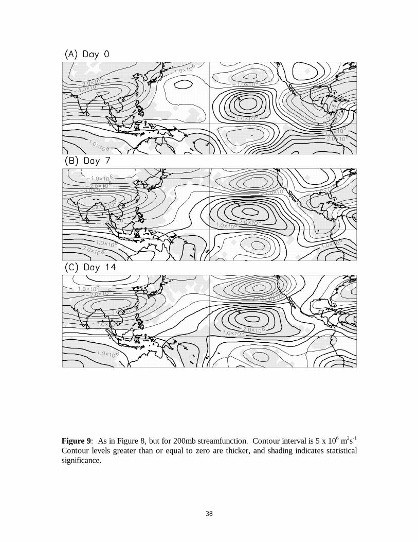
Lag-regression of the CPV on 7-day running mean 200 hPa streamfunction is used
to illustrate the evolution of the large-scale low frequency circulation field (Fig. 9). An
upper tropospheric cyclone, with associated tropical westerly wind anomalies propagates
eastward out of the Indian Ocean along with the suppressed convection. An upper
tropospheric cyclone in the Eastern Pacific develops after the flare-up of convection east

13
of the dateline. This trough strengthens and moves slightly eastward between days 0 and
14.
The growth of anomalous upper-tropospheric westerlies in the Eastern Pacific
occurs simultaneously with the onset of precipitation in California. We hypothesize that
the mechanism for California rainfall enhancement is related to the steering effect of these
westerlies on synoptic-scale weather systems in the Eastern Pacific. To illustrate this, we
have used 7-day running mean high-pass filtered 850 hPa meridional wind variance as a
proxy for synoptic-eddy activity. The high-pass filter used is simply the deviation of daily
averages from five-day running means. Lag-regression maps (Fig. 10) show that there is a
significant enhancement of synoptic-eddy activity off the coast of California in the two
weeks after a positive projection of tropical OLR on the leading canonical predictor
vector. We hypothesize that the development of the OLR anomalies associated with the
CPV (Figure 8a) force upper-tropospheric westerly wind anomalies in the far eastern
Pacific. These westerly wind anomalies act to steer weather systems farther east than
usual, allowing them to reach the California coast rather than occluding and decaying in
the Gulf of Alaska. The fact that both the tropical OLR anomalies and the associated
upper tropospheric westerlies are fairly persistent once established leads to the
predictability of California rainfall in the two week range shown in Fig. 3.
The OLR field associated with the CPV (Fig. 8) is fairly complicated. From a
monitoring perspective, it would be useful to know which features are primarily
responsible for the upper tropospheric wind signal in the Eastern Pacific. Fig. 8a shows
that during times when there is a positive projection on the leading canonical predictor
vector there are typically two opposite signed OLR anomalies, one located in the

14
equatorial Indian Ocean and one near 5oS east of the dateline. Here we use two indices
that measure the strength of tropical convection in these two regions to identify the
extratropical circulation features associated with each separately. The goal is to
understand the relative roles of convection in these two regions in producing the
California rain signal two weeks later. The indices we use are based on a rotated EOF
analysis of the OLR data. As a measure of the Indian Ocean convection we use the
expansion coefficient for rotated EOF 2, and for the eastern Pacific convection we use a
linear combination of the expansion coefficients of rotated EOFs 5 and 9 (not shown).
The OLR field regressed on these two indices (Fig. 11) shows that they indeed do capture
the essential aspects of the OLR field typically associated with the CPV. The 200 hPa
streamfunction field regressed on these two indices at two week lag (Fig. 12) show that,
although both the Indian Ocean and eastern Pacific convective anomalies are associated
with enhanced upper level westerlies off the coast of California two weeks later, enhanced
convection in eastern Pacific is contributing much more to the total westerly wind signal
associated with the CPV (Fig. 9c) than suppressed convection in the Indian Ocean.
Therefore, we conclude that it is enhanced convection east of the dateline near 5oS that is
the primary feature associated with the CPV that is responsible for the precipitation signal
in California two weeks later. These results are in qualitative agreement with previous
studies of the linear, steady state response to idealized tropical heating distributions (such
as Ting and Yu, 1998), although there are significant differences in detail. For example,
the upper tropospheric westerly wind signal off the coast of California is considerably
farther east than linear, steady state dynamics would predict. This is likely due to

15
processes typically not represented in linear models, such as transient-eddy feedback, and
to the restrictions imposed by the steady-state assumption.
5. Results with California rain-gauge data.
All of the results presented so far have used reanalysis precipitation as the
predictand. As discussed in section 2, reanalysis precipitation is not directly constrained
by observations, and therefore is subject to the limitations and biases of the assimilating
model. In this section we present results with daily California precipitation gauge data as
a predictand. We choose California because the results with reanalysis precipitation
suggest that it is the region with the strongest predictable signal where gauge data is
available.
Weekly California precipitation station data for the 24 winters between 1974/75
and 1998/99 (excluding 1978/79) is used. The data is derived from the daily precipitation
dataset described by Eischeid et al (2000). 442 stations are available in California for this
time period. As a predictand we use an average of all the stations in the Central and
Southern Coast drainage climate divisions. The results are not significantly different if
either of the two climate divisions is used alone, or if a multivariate analysis is performed
using all California climate divisions. As before, a probability-integral transform is applied,
and the daily climatology is removed. This yields an index of coastal California
precipitation which is Gaussian distributed. Since the predictand is now a scalar, the CCA
reduces to finding a vector representing the covariance between the leading 20 normalized
PCs of tropical OLR and the normalized coastal California precipitation index two weeks

16
later. The predictor index is then simply the projection of the observed OLR PCs on to
this vector. Cross-validation is used so that for a given winter season, only data from the
other 23 winters is used to compute the covariance vector.
The rank-order correlation between the OLR predictor index and the coastal
California precipitation index two weeks later is 0.2, which is comparable to that obtained
with reanalysis precipitation (Fig. 3). Lag-regression of the 7-day running mean tropical
OLR on to the OLR predictor index (not shown) yields an evolution very similar to that
associated with the leading canonical predictor variable for reanalysis precipitation (Fig.
8). This indicates that reanalysis, at least in winter, does provide a reasonable estimate of
precipitation variability in this region on weekly timescales. Fig. 13a shows the changes
in the probability of above, below and near normal coastal California precipitation
associated with extreme values of the predictor index. The risk of above normal weekly
rainfall in coastal California is increased by 33%, relative to the climatological probability,
when the OLR predictor index is in the upper quintile. Conversely, the risk of below
normal precipitation is reduced by 66%. Similar results are obtained for below normal
rainfall when the predictor is in the lower quintile. These results are very similar to that
obtained for reanalysis precipitation in the California region (Fig. 4). Therefore, we
conclude that the results presented here with reanalysis estimated precipitation provide a
realistic estimate of the week two predictability of actual rainfall along the West Coast of
North America associated with subseasonal tropical OLR variations.
6. Summary and conclusions.

17
Subseasonal variations of tropical convection can be used to improve the skill of
two-week precipitation forecasts over western North America, and particularly in
California. The level of skill obtained from a simple linear statistical model is comparable
to that provided by current numerical forecasts (which do not accurately simulate
subseasonal tropical convective variability). Using a weekly ENSO index as a predictor of
California precipitation two weeks later also yields a similar level of skill. However, since
the effect of ENSO on tropical convection is fairly well represented in numerical weather
prediction models (Barsugli et al 1999), a weekly ENSO index does not yield additional
predictive information. Most of the results presented here utilize reanalysis precipitation
as a predictand, although similar levels of skill were shown using California rain-gauge
data.
The dynamical mechanism associated with this predictability is primarily related to
the remote forcing of upper tropospheric westerly wind anomalies just off the coast of
California by enhanced tropical convection just south of the equator and east of the
dateline. Synoptic-scale weather systems which would otherwise occlude and decay in the
Gulf of Alaska are steered farther east toward the California coast by these enhanced
westerlies. Anomalous tropical convection in the eastern equatorial Indian Ocean also
plays a similar role in the prediction of California rainfall, although its impact on upper
tropospheric westerlies in the Eastern Pacific is much weaker.
Higgins et al. (2000) have examined the relationship between extreme three-day
precipitation totals along the West Coast of the United States and concurrent intraseasonal
tropical OLR patterns. They found that extreme precipitation events in Southern
California tend to be associated with enhanced tropical convection between 150oE and the

18
dateline, and suppressed convection just east of the dateline. This is quite different that
the pattern of tropical OLR which we find is associated with the highest predictability of
California rainfall two weeks later. We attribute this difference to the fact that our
analysis is designed to pick out patterns of OLR and West Coast precipitation that have
the highest correlation at two week lag, while the compositing used by Higgins et al
(2000) will reveal the pattern of OLR that tends to occur simultaneously with heavy
precipitation along the West Coast. These patterns need not be the same, and the fact
that they are not implies that the precipitation events in the Higgins et al (2000) composite
are not predictable two weeks in advance using tropical OLR information alone.
Jones (2000) has examined the relationship between the Madden-Julian (MJO)
oscillation (as defined by the leading two EOFS of 20-90 day bandpass filtered OLR) and
the frequency of extreme rainfall events in California. He found an increased frequency of
extreme events when the MJO was active. Our analysis uses the first 20 PCs of tropical
OLR, and therefore includes more than just the MJO. In fact, the leading canonical
predictor vector does not project very strongly on the first two EOFs of OLR, more than
10 EOFs are needed to represent its structure. In order to assess the relative importance
of the MJO, as opposed to other modes of subseasonal tropical convective variability, we
have redone the CCA using only the first two PCs of OLR. Fig. 14 shows the rank-order
correlation between the resulting leading canonical variable (which is primarily the leading
OLR PC) and the reanalysis precipitation two weeks later. Comparing with Fig. 3, it is
evident that the region of maximum predictability associated with the MJO is located over
the southwest U.S., instead of off the coast of California. When viewed as a domain
average, the predictability associated with the MJO is a relatively small portion of the total

19
predictability associated with subseasonal tropical convective variability. However, locally
in southern California and the southwest U.S., the MJO appears to be producing most of
the predictable precipitation signal. Therefore, we conclude that although the MJO may
be a useful predictor of rainfall in southern California and the desert Southwest, there are
other important aspects of subseasonal tropical convective variability that should be taken
into account when making predictions over a larger area.
In this study we have shown that subseasonal tropical convective activity is linearly
related to rainfall near the West Coast of North America two weeks later, and that this
linear relationship can be used to improve precipitation predictions. However, we have
not proven that the predictability is ultimately rooted in tropical processes, since the
possibility remains that the OLR anomalies shown in Fig. 8a are being forced by
circulation features of mid-latitude origin. To examine this question, we have produced
CCA forecasts using streamfunction at 250 and 850 hPa, in the region 15-70oN and 60oE
to 120oW, as a predictor. The computational procedure is the same as outlined in section
2, but instead of using 20 EOFs of tropical OLR as predictors, we use the first 20 EOFs of
the combined vector of 250 and 850 hPa streamfunction (with ENSO linearly removed).
Fig 15 shows the rank correlation between week two forecast (using all 20 canonical
predictor vectors) and analyzed reanalysis precipitation, using tropical OLR as a predictor
(Fig 15a), Northern Hemisphere extratropical streamfunction as a predictor (Fig. 15b),
and extratropical streamfunction with the tropical OLR signal (as defined by the first 20
EOFs) linearly removed (Fig. 15c). Comparing Fig. 15a with Fig 15b, it is clear that a
large part of the predictable precipitation signal along the West Coast cannot be captured
using the extratropical circulation alone. Furthermore, Fig. 15c shows there is virtually no

20
predictive utility in that part of the circulation that is independent of tropical OLR, at least
along the West Coast. Although we have not addressed the ultimate origin of the tropical
OLR patterns shown in Fig. 8, if they were primarily forced by mid-latitude circulation
anomalies, we would have expected forecasts of West Coast precipitation using mid-
latitude circulation as a predictor to be at least as skillful as those using tropical OLR.
These results suggest that most of the predictable signal in West Coast precipitation is
related to tropical processes at two week lag. Although the mid-latitude circulation alone
can be used to make skillful forecasts, most of the skill comes from that part of the
circulation that is linearly related to (and most likely forced by) tropical convective
processes.
The statistical model used here is linear, and does not use any mid-latitude
circulation information. Presumably, the remote impacts of tropical convection may be
affected by mid-latitude flow conditions, particularly in the vicinity of the Pacific Jet.
Numerical weather prediction models, if they were able to accurately simulate subseasonal
tropical convective variability, could conceivably exploit such nonlinear tropical-
extratropical interactions. Therefore, the skill of statistical predictions presented here
may be considered a lower bound on the potential for improved predictability of West
Coast rainfall in the week two range. Until numerical models can better simulate tropical
variability on subseasonal timescales, they should be augmented with statistical models,
which provide essentially independent information associated with the state of tropical
convection at the initial time. Exactly how to combine the output of statistical and
numerical models to exploit the predictive information inherent in satellite measurements
of tropical convection is an active area of research.

21
Acknowledgements: Support for this research was provided by the U.S. CLIVAR
PanAmerican Climate Studies program (PACS). We thank Dr. Matthew Newman for
helpful discussions on the finer points of linear regression and SVD, and two anonymous
reviewers for insightful comments.

22
Figure Captions:
Figure 1: Standard deviation of 7-day averaged, spectrally smoothed OLR with ENSO
linearly removed. Contour interval is 2 Wm-2. Values greater than 14 Wm-2 are shaded.
The boxed region is the domain used for the CCA.
Figure 2: Standard deviation of weekly, spectrally smoothed precipitation from
reanalysis. Contour interval is 2 mm. Values greater than 21 mm are shaded. The boxed
region is the domain used for the CCA.
Figure 3: The rank-order correlation between the leading canonical predictor variable
(computed using the leading 20 PCs of tropical OLR) and the analyzed precipitation two
weeks later. Positive contours are thicker, the zero line is omitted and shading indicates
statistical significance.
Figure 4: Risk (relative to climatological risk of 33%) of precipitation being in the upper
tercile given that the leading canonical predictor variable two weeks prior is in the upper
(A) or lower (B) quintile. Shaded areas are significantly different than 1.0 at the 95%
level, thicker contours are greater than 1.0. Contour interval is 0.1, and only contours less
than 0.9 and greater than 1.1 are plotted.

23
Figure 5: The rank-order correlation between a weekly ENSO index (the leading PC of
tropical SST) and analyzed precipitation two weeks later. Positive contours are thicker,
the zero line is omitted, and shading indicates statistical significance.
Figure 6: (A) rank-order correlation between analyzed and operational ensemble mean
week two forecast precipitation for four winters (1996/1997 - 1999/2000). (B) rank-order
correlation between analyzed precipitation and leading canonical predictor variable two
weeks prior for same time period (which is different than the time period used to compute
Fig. 3). Positive contours are thicker, the zero line is omitted, and shading indicates
statistical significance.
Figure 7: Map of leading canonical predictor vector, representing tropical OLR. Positive
contours are thicker, and the zero line is omitted.
Figure 8: OLR regressed on leading canonical predictor variable at lag 0 (A), 7 (B) and
14 (C) days. Maps are scaled for one standard deviation of the canonical predictor
variable. Contour interval is 1.5 Wm-2. Positive contours are thicker, the zero line is
omitted and shading indicates statistical significance. Day 0 is the initial time for CCA
forecasts, and day 14 is the forecast verification time.
Figure 9: As in Figure 8, but for 200 hPa streamfunction. Contour interval is 5 x 10⁶
m2s-1 Contour levels greater than or equal to zero are thicker, and shading indicates
statistical significance.

24
Figure 10: As in Figure 8, but for 850mb high-pass meridional wind variance. Contour
interval is 1 m2s-2. Positive contours are thicker, the zero line is omitted, and shading
indicates statistical significance.
Figure 11: OLR regressed on indices of Indian Ocean (A) and eastern Pacific (B)
convection. Contour interval 1.5 Wm-2. Positive contours are thicker, the zero line is
omitted, and shading indicates statistical significance.
Figure 12: 200 hPa streamfunction regressed on indices of Indian Ocean (top panel) and
eastern Pacific (bottom panel) convection at two-week lag. Contour interval 5 x 10⁶ m2s-
1. Contour levels greater than or equal to zero are thicker, and shading indicates statistical
significance.
Figure 13: (A) Conditional tercile probabilities for observed coastal California weekly
precipitation when the OLR predictor index two weeks prior is in the upper and lower
quintiles of its distribution. The OLR predictor is constructed as described in section 5,
using the first 20 EOFs of tropical weekly OLR (with ENSO linear removed). (B)
Conditional tercile probabilities for a persistence forecast (where the predictor is the
observed weekly California rainfall two weeks prior).
Figure 14: As in Fig. 3, but for a canonical predictor variable computed using only the
leading two PCs of tropical OLR.
25
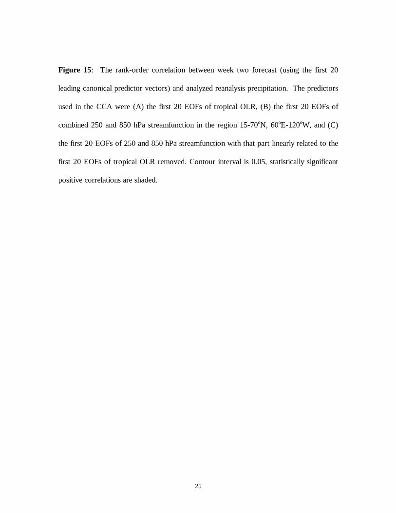
Figure 15: The rank-order correlation between week two forecast (using the first 20
leading canonical predictor vectors) and analyzed reanalysis precipitation. The predictors
used in the CCA were (A) the first 20 EOFs of tropical OLR, (B) the first 20 EOFs of
combined 250 and 850 hPa streamfunction in the region 15-70oN, 60oE-120oW, and (C)
the first 20 EOFs of 250 and 850 hPa streamfunction with that part linearly related to the
first 20 EOFs of tropical OLR removed. Contour interval is 0.05, statistically significant
positive correlations are shaded.

26
References:
Barnett, T. P., and R. W. Preisendorfer, 1987: Origins and levels of monthly and seasonal
forecast skill for United States surface air temperatures determined by canonical
correlation analysis. Mon. Wea. Rev., 115, 1825-1850.
Barnston, A. G., A. Leetma, V. E. Kousky, R. E. O’Lenic, H. van den Dool, A. J.
Wagner, and D. A. Unger, 1999: NCEP forecasts of the El Nino of 1997/98 and its U.S.
Impacts. Bull. Amer. Meteor. Soc., 80, 1829-1852.
Barsugli, J. J., J. S. Whitaker, A. F. Loughe, and P. D. Sardeshmukh, 1999: Effect of the
1997/98 El Nino on individual large-scale weather events. Bull. Amer. Meteor. Soc., 80,
1399-1411.
Bretherton, C. S., Smith, C., and J. M. Wallace, 1992: An intercomparison of methods
for finding coupled patterns in climate data. J. Climate, 5, 541-560.
Eischeid, J.K, P. Pasteris, H.F. Diaz, M. Plantico, and N. Lott, 2000: Creating a serially
complete, national daily time series of temperature and precipitation for the United States.
J.Appl. Met., 39, 1580-1591.

27
Hendon, H., B. Liebmann, M. Newman, and J. D. Glick, 2000: Medium-range forecast
errors associated with active episodes of the Madden-Julian oscillation. Mon. Wea. Rev.,
128, 69-86.
Higgins, R. W., J.-K. E. Schemm, W. Shi, and A. Leetma, 2000: Extreme precipitation
events in the Western United States related to tropical forcing. J. Climate, 13, 793-820.
Jones, C., 2000: Occurrence of extreme precipitation events in California and
relationships with the Madden-Julian oscillation. J. Climate, to appear.
Kalnay, E. and Coauthors, 1996: The NCEP/NCAR 40 year reanalysis project. Bull.
Amer. Meteor. Soc., 77, 437-471.
Liebmann, B., and C. A. Smith, 1996: Description of a complete (interpolated) outgoing
longwave radiation dataset. Bull. Amer. Meteor. Soc., 77, 1275-1277.
Madden, R. A., 1989: On predicting probability distributions of time-averaged
meteorological data. J. Climate, 2, 922-935.
Mo, K. C., and R. W. Higgins, 1998a: Tropical influences on California precipitation. J.
Climate, 11, 412-430.

28
Mo, K. C., and R. W. Higgins, 1998b: Tropical convection and precipitation regimes in
the Western United States. J. Climate, 11, 2404-2423.
Newman, M., P. D. Sardeshmukh, and J. D. Bergman, 2000: An assessment of the
NCEP, NASA, and ECMWF reanalyses over the tropical West Pacific warm pool. Bull.
Amer. Meteor. Soc., 81, 41-48.
Press, W. H., B. P Flannery, S. A. Teukolsky, and W. T. Vettering, 1989: Numerical
Recipes: The Art of Scientific Computing. Cambridge University Press. 702pp.
Sardeshmukh, P. D., G. P. Compo, and C. Penland, 2000: Changes in probability
associated with El Nino. J. Climate, to appear.
Sardeshmukh, P. D., and B. J. Hoskins, 1984: Spatial smoothing on the sphere. Mon.
Wea. Rev., 112, 2524-2529.
Schohner, T., and S. E. Nicholson, 1989: The relationship between California rainfall and
ENSO events. J. Climate, 2, 1258-1269.
Ting, M., and L. Yu, 1998: Steady response to tropical heating in wavy linear and
nonlinear baroclinic models. J. Atmos. Sci., 55, 3565-3582.

29
Toth, Z., and E. Kalnay, 1993: Ensemble forecasting at NMC: The generation of
perturbations. Bull. Amer. Meteor. Soc., 74, 2317-2330.
Waliser, D. E., C. Jones, J.-K. Schemm, and N. E. Graham, 1999: A statistical extended-
range tropical forecast model based on the slow evolution of the Madden-Julian
oscillation. J. Climate, 12, 1918-1939.
Wilks, D. S., 1995: Statistical Methods in Atmospheric Sciences. Academic Press,
467pp.
Winkler, C. R., M. Newman, and P. D. Sardeshmukh: 2000: A linear model of
wintertime low-frequency variability. Part I: Formulation and forecast skill. J. Climate,
submitted.
Wolter, K., R. M. Dole, and C. A. Smith, 1999: Short-term climate extremes over the
continental United States and ENSO. Part I: Seasonal temperatures. J. Climate, 12,
3255-3272.

30
Figure 1: Standard deviation of 7-day averaged, spectrally smoothed OLR with ENSOlinearly removed. Contour interval is 2 Wm-2. Values greater than 14 Wm-2 are shaded.The boxed region is the domain used for the CCA.

31
Figure 2: Standard deviation of weekly, spectrally smoothed precipitation fromreanalysis. Contour interval is 2 mm. Values greater than 21 mm are shaded. The boxedregion is the domain used for the CCA.

32
Figure 3: The rank-order correlation between the leading canonical predictor variable(computed using the leading 20 PCs of tropical OLR) and the analyzed precipitation twoweeks later. Positive contours are thicker, the zero line is omitted and shading indicatesstatistical significance.

33
Figure 4: Risk (relative to climatological risk of 33%) of precipitation being in the uppertercile given that the leading canonical predictor variable two weeks prior is in the upper(A) or lower (B) quintile. Shaded areas are significantly different than 1.0 at the 95%level, thicker contours are greater than 1.0. Contour interval is 0.1, and only contours lessthan 0.9 and greater than 1.1 are plotted.

34
Figure 5: The rank-order correlation between a weekly ENSO index (the leading PC oftropical SST) and analyzed precipitation two weeks later. Positive contours are thicker,the zero line is omitted, and shading indicates statistical significance.

35
Figure 6: (A) rank-order correlation between analyzed and operational ensemble meanweek two forecast precipitation for four winters (1996/1997 - 1999/2000). (B) rank-ordercorrelation between analyzed precipitation and leading canonical predictor variable twoweeks prior for the same time period. Positive contours are thicker, the zero line isomitted, and shading indicates statistical significance.

36
Figure 7: Map of leading canonical predictor vector, representing tropical OLR. Positivecontours are thicker, and the zero line is omitted.

37
Figure 8: OLR regressed on leading canonical predictor variable at lag 0 (A), 7 (B) and14 (C) days. Maps are scaled for one standard deviation of the canonical predictorvariable. Contour interval is 1.5 Wm-2. Positive contours are thicker, the zero line isomitted and shading indicates statistical significance. Day 0 is the initial time for CCAforecasts, and day 14 is the forecast verification time.
38
Figure 9: As in Figure 8, but for 200mb streamfunction. Contour interval is 5 x 10⁶ m2s-1
Contour levels greater than or equal to zero are thicker, and shading indicates statisticalsignificance.

39
Figure 10: As in Figure 8, but for 850mb high-pass meridional wind variance. Contourinterval is 1 m2s-2. Positive contours are thicker, the zero line is omitted, and shadingindicates statistical significance.

40
Figure 11: OLR regressed on indices of Indian Ocean (A) and eastern Pacific (B)convection. Contour interval 1.5 Wm-2. Positive contours are thicker, the zero line isomitted, and shading indicates statistical significance.

41
Figure 12: 200 hPa streamfunction regressed on indices of Indian Ocean (top panel) andeastern Pacific (bottom panel) convection at two-week lag. Contour interval 5 x 10⁶ m2s-
1. Contour levels greater than or equal to zero are thicker, and shading indicates statisticalsignificance.

42
0
10
20
30
40
50
predictor in lower quintilepredictor in upper quintile
prob
abili
ty
precip categorybelow normal near normal above normal
(A) CCA Forecast
0
10
20
30
40
50
predictor in lower quintilepredictor in upper quintile
precip category
below normal near normal above normal
(B) Persistence Forecast
prob
abili
ty
Figure 13: (A) Conditional tercile probabilities for observed coastal California weeklyprecipitation when the OLR predictor index two weeks prior is in the upper and lowerquintiles of its distribution. The OLR predictor is constructed as described in section 5,using the first 20 EOFs of tropical weekly OLR (with ENSO linear removed). (B)Conditional tercile probabilities for a persistence forecast (where the predictor is theobserved weekly California rainfall two weeks prior).

43
Figure 14: As in Fig. 3, but for a canonical predictor variable computed using only theleading two PCs of tropical OLR.

44
Figure 15: The rank-order correlation between week two forecast (using the first 20leading canonical predictor vectors) and analyzed reanalysis precipitation. The predictorsused in the CCA were (A) the first 20 EOFs of tropical OLR, (B) the first 20 EOFs ofcombined 250 and 850 hPa streamfunction in the region 15-70oN, 60oE-120oW, and (C)the first 20 EOFs of 250 and 850 hPa streamfunction with that part linearly related to thefirst 20 EOFs of tropical OLR removed. Contour interval is 0.05, statistically significantpositive correlations are shaded.