Successful adaptation to 3D inversion methodologies for ... · Successful adaptation to 3D inversion methodologies for archaeological-scale, ... English Heritage, ... The rst term

submitted to Geophys. J. Int.

Successful adaptation to 3D inversion methodologies

for archaeological-scale, total field magnetic datasets

S. Cheyney1 ?, S. Fishwick1, I. Hill1, N. Linford2

1 Department of Geology, University of Leicester, University Road, Leicester, LE1 7RH, UK

2 Geophysics Team, English Heritage, Fort Cumberland, Eastney, Portsmouth, PO4 9LD, UK

SUMMARY

Despite the development of advanced processing and interpretation tools for magnetic

datasets in the fields of mineral and hydrocarbon industries, these methods have not

achieved similar levels of adoption for archaeological or very near surface surveys.

Using a synthetic dataset we demonstrate that certain methodologies and assumptions

used to successfully invert more regional-scale data can lead to large discrepancies

between the true and recovered depths when applied to archaeological-type anomalies.

We propose variations to the current approach, analysing the choice of the depth-

weighting function, mesh design and parameter constraints, to develop an appropriate

technique for the 3D inversion of archaeological scale datasets. The results show a

successful recovery of a synthetic scenario, as well as a case study of a Romano-Celtic

temple in the UK. For the case study, the final susceptibility model is compared with

two coincident ground penetrating radar surveys, showing a high correlation with the

comparative depth slices. The new approach takes interpretation of archaeological

datasets beyond a simple 2D visual interpretation based on pattern recognition.

Key words: magnetic anomalies: modelling and interpretation, inverse theory, near-

surface, archaeology.

2 S. Cheyney et al.

1 Introduction

Archaeological excavation can be expensive and slow, and damages the material excavated in an

unrecoverable way, therefore while it is essential for understanding buried historical structures,

excavation must be applied very selectively. Geophysical surveys have become increasingly com-

mon in archaeological prospection, and are typically used to guide the targeted positioning of

excavations. Due to the ability to survey large areas rapidly whilst being able to detect subtle

variations in the properties of the subsurface, magnetic surveying has now become one of the

most commonly used geophysical techniques over archaeological sites. For the majority of any

site, these results will be the only evidence of the full spatial extent of the buried structures.

Typically, interpretation is done visually using optimised images of the raw data. More ad-

vanced processing and interpretation steps can be implemented to improve the clarity of the

dataset, or produce a transformation that will aid interpretation. The use of derivative-based

methods such as the horizontal gradient magnitude (Cordell & Grauch 1985), analytic signal

(Nabighian 1972), theta map (Wijns et al. 2005) and tilt angle (Miller & Singh 1994) are all

shown to derive information regarding the horizontal location of anomalies, while Source Pa-

rameter Imaging (Thurston & Smith 1997) and Euler deconvolution (Reid et al. 1990) have

been demonstrated to produce depth estimates to certain types of subsurface structures. The

use of gradient based methods to exploit magnetic data has gained significant popularity in

aero-magnetic regional and mineral exploration surveys. Their direct implementation in archae-

ological survey interpretation remains rare, due to the particular challenges posed due to the

low amplitude and high-wavenumber content of archaeological magnetic surveys (Cheyney et al.

2011).

The ideal solution is a full 3D inversion of the magnetic total field, to estimate the distribution

of subsurface magnetic susceptibility. Alongside the low signal to noise level, there are two other

significant challenges associated with inversion of archaeological-scale datasets. These are, the

effects of regional trends and their incorporation into the mesh design, and secondly, the reality

that archaeological anomalies will often consist of positive and negative susceptibility contrasts

with the host material, that requires the interpretation to incorporate both positive and negative

apparent susceptibilities.

Here, we demonstrate a successful implementation of the MAG3D inversion code (UBC-GIF

2005) for the inversion of high resolution total field data, consisting of anomalies of just a few nT.

While an unconstrained inversion with default parameters can easily produce an interpretation

that fits the data, it is unlikely to be an appropriate representation of an archaeological site. By

? [email protected]

3D inversion of archaeological-scale magnetic data 3

applying a methodology that places appropriate constraints on the inversion, a robust solution

can be produced even where no a priori information is available. The method is tested using a

case study of a Romano-Celtic temple near Silchester, UK, and compared to an earlier ground

penetrating radar survey (Linford et al. 2010).

1.1 Archaeological anomalies

Magnetic anomalies measured at the surface are indicative of a susceptibility contrast between

the archaeological feature and the surrounding material (eg. soil). The magnitude of these anoma-

lies will therefore depend on the absolute susceptibility of both the host material as well as the

feature of interest. Anthropogenic land-use has been shown to often lead to an enhanced and

variable magnetic susceptibility in the upper soil level (Le Borgne 1955; Linford 2004; Fassbinder

et al. 1990; Maher & Taylor 1988). For the same type of feature, the anomaly and subsequent

susceptibility contrast may be more dependant on the host material than the anomalous feature

itself.

Data from archaeological magnetic surveys typically reveal both positive and negative anoma-

lies, as both positive and negative contrasts to the surrounding soil susceptibility can be present.

Positive contrasts are typical in areas where ditches or other intrusions have been cut into top

soil that has undergone enhancement of susceptibility (Linford 2006). Negative anomalies can

be formed in a similar way with foundations and walls consisting of a low-susceptibility rock

such as limestone, or where the ditches have been cut into high susceptibility soils and infilled

with low-susceptibility alluvium (Aspinall et al. 2008). This scenario of incorporating both posi-

tive and negative susceptibility into the interpretation is uncommon for mineral and exploration

surveys, and invalidates an assumption of a single polarity that is often invoked to simplify the

interpretation.

1.2 Estimating subsurface susceptibility: previous work

Interpreting the magnetic field by way of a varying susceptibility model of the subsurface has

been limited in the past by the computer power required, and the problems associated with

identifying the ‘most-likely’ model from the many solutions that will produce a good fit to the

observations. Several methods have been developed that optimise a pre-defined structure to fit

the data, such as a dyke or fault model for geology (Powell 1967), or modelling of pit houses

in an archaeological context (Herwanger et al. 2000). These methods significantly reduce the

complexity of the inversion algorithm, however the input structure and susceptibility contrasts

chosen have a significant effect on the final model, and therefore limits the applicability of the

approach to when a lot of a priori information is available.

4 S. Cheyney et al.

Where the target shape is unknown, it is required to represent the subsurface by a less

prejudiced, more generalised structure. Eder-Hinterleitner et al. (1995) achieved this by forming

a subsurface consisting of a 3-dimensional grid of dipoles, whereas Dittmer & Szymanski (1995)

used a mesh of voxels, or cells. Both techniques allowed only a finite number of susceptibilities

to be used. These methodologies proved successful, but heavily influenced by the suitability of

the chosen parameters.

Generalised inversion schemes involving dividing the subsurface into a 3-dimensional mesh

were developed initially for mineral exploration purposes (Li & Oldenburg 1996; Pilkington

1997). These approaches have the advantage that they can still be implemented in situations

where no a priori information regarding the source shape or susceptibility is available. Instead,

the final susceptibility distribution is controlled by choices regarding how smoothly varying the

final interpretation should be, the polarity of the recovered features, and the likely continuity of

features in certain directions. Variations of this method have been developed for high susceptibil-

ity cases (Lelievre & Oldenburg 2006), and alternative approaches based of spectral and wavelet

analyses have also been proposed for inversion of the subsurface properties (Li & Oldenburg

2003; Ravat et al. 2007; Saracco et al. 2007).

The principles in the Li & Oldenburg (1996) paper, were later adapted at the University of

British Columbia Geophysical Inversion Facility (UBC-GIF) to produce a commercially available

program called MAG3D (UBC-GIF 2005). Li & Oldenburg (1996) employ the method to model

copper-gold porphyry deposits in central British Columbia, and Williams (2008) shows how the

addition of geological constraints can be used to refine the resultant model from the Agnew-

Wiluna greenstone belt and Perseverance nickel deposit in Australia. MAG3D has also been

implemented in archaeological situations by Piro et al. (2007), where chamber tombs at the

Sabine Necropolis of Colle del Forno in Rome, Italy, were inverted using the vertical gradient of

the magnetic field. Piro et al. (2007) noted that modelling both positive and negative apparent

susceptibility contrasts would be a limit to further archaeological uptake to the method. Another

example of an archaeological implementation can be seen in Sheriff et al. (2010), for investigation

of late 19th century, early 20th century building foundations in Yellowstone, USA. The nature of

these anomalies result in amplitudes of hundreds of nT, and related large susceptibility contrasts

to the surrounding area, whilst again dealing with just a single, positive susceptibility contrast

with the host material.

1.3 Methodology

We use the MAG3D software (UBC-GIF 2005) to produce models of the subsurface. In the

following section we discuss some of the key aspects of the inversion routine given the particular


challenges of inverting archaeological-scale magnetic data. For a more complete discussion of the

inversion approach see Li & Oldenburg (1996).

The MAG3D inversion routine seeks to produce a final model by minimising the following

objective function:

φ(m) = φd + βφm (1)

where φd is the data-misfit, φm is the model norm and β is the trade-off, or regularisation

parameter. Choosing a low value of β will produce a model that preferentially fits the data, while

a high value of β will place a higher emphasis on meeting the requirements of the model-norm

rather than a good fit to the observed data.

The data-misfit is defined as:

φd =

N∑j=1

(dobsj − F [m]

εj

)2

(2)

F [m] is the calculated forward modelled data, dobsj are the observed field measurements,

and εj is the standard deviation of the j′th datum. The noise is assumed to be Gaussian and

independent of the datum amplitude. If the level of noise in the data is over-estimated or under-

estimated, it is possible to compensate for this in the choice of β.

Should knowledge of the subsurface be available, it may be desirable to manipulate the

model norm to calculate a model as close as possible to this. MAG3D does this by including a

reference model in the model norm. The model norm is declared by Li & Oldenburg (1996) as:

φm(m) = αs

∫vws{w(z)[m−mref ]}2dv + αx

∫vwx

{∂w(z)[m−mref ]

∂x

}2

dv

+αy

∫vwy

{∂w(z)[m−mref ]

∂y

}2

dv + αz

∫vwz

{∂w(z)[m−mref ]

∂z

}2

dv

(3)

The first term of Equation 3 controls the smallness of the model, which is how closely the

model matches the reference model, mref , or a zero-halfspace if no reference model is provided.

The constants αs, αx, αy, and αz control the relative importance of each term. Should there be

a preference for constraining smallness or smoothness between individual cells in the mesh, this

can be controlled by ws, wx, wy, and wz. These are spatially dependent sensitivity weighting

functions, and unlike the α-parameters which are single values, w-parameters are declared for

each cell boundary within the mesh. The function w(z) is a depth weighting function that will

be discussed in more detail in the following section.

6 S. Cheyney et al.

A simple and commonly used approach to constraining the model output from the inversion

routine is to attempt to recover a smooth variation in the susceptibility throughout the model.

This is often used where no other a priori information exists, where the simplest explanation

of the observations is the most reasonable. This approach may not be suitable for archaeologi-

cal purposes. Anomalies present in archaeological magnetic data are usually caused by abrupt

changes in the subsurface properties caused by human activity, such as the case with foundation

materials, or infill where ditches have been filled over time with soil of contrasting magnetisation.

Either scenario is unlikely to result in a gradual change in magnetisation, and the smooth-model

constraint may not be appropriate (Piro et al. 2007). It was important to this research to identify

the effects that the smoothing parameters αx, αy, and αz have on the resulting models. Employ-

ing smoothing parameters reduces the likelihood of recovering irregular structures in the model,

and may be useful in the presence of excessive noise. Smoothing in the vertical direction by way

of varying αz has been observed to be less beneficial. Archaeological remains are often buried

relatively shallow in the subsurface and running the inversion with vertical smoothing often

yields results where anomalies are continuous to the surface, and no discrete depths can be ob-

served. Where anomalies are present at multiple depths for the same lateral position smoothing

often prevents the vertical separation and therefore the interpretation of archaeological layering.

Our findings support the observation made by Piro et al. (2007) that the smallest model should

be sought for archaeological scenarios. Design of an appropriate reference model is found to be

critical for the successful implementation of an inversion of archaeological data.

A common assumption made for magnetic inversion is that all the magnetisation is induced.

Magnetisation can be locked into materials such as kilns, ovens, baked floors and fired bricks.

Heating these materials results in a high thermal remanent magnetisation that may be in a

different direction to the inducing field. In these scenarios the distribution of the recovered mag-

netic susceptibility is likely to be significantly affected by the incorrect magnetisation vector

and the result will not be reliable. Anthropogenic land-use often leads to an enhanced concen-

tration of magnetic minerals close to the superparamagnetic/single domain boundary in the

upper soil level due to the presence of high concentrations of iron oxides. Enhancement of the

subsurface develops through a range of mechanisms, including the reduction of haematite to the

more magnetic form magnetite, and thus raising the magnetic susceptibility of the soil (Maher

& Taylor 1988; Linford 2004). Due to the fine magnetic grain size of the neo-formed minerals a

viscous magnetic remanence can often occur following the direction of the inducing field. Labo-

ratory measurements using dual frequency magnetic susceptibility meters show that for typical

archaeological soils an increase of 45% in magnetisation can occur in a time period of 100-1000s

(Graham & Scollar 1976). Inverting the data in these scenarios is likely to successfully recover


the spatial distribution of anomalies, but will result in an anomalously higher magnetisation

than would otherwise be the case.

2 Synthetic modelling

Here, a synthetic scenario has been designed to optimise the use of MAG3D for archaeological

purposes. This has focussed on three key areas; the depth-weighting w(z) of the inversion, the

mesh design, and the modelling of both positive and negative apparent susceptibility contrasts.

2.1 Depth weighting

Performing the inversion without a depth weighting function present in the objective function

would result in anomalous susceptibility values being modelled towards the top of the mesh.

In the absence of an a priori reference model, placing the anomalies at the shallowest depths

requires the smallest values over the smallest volume, and therefore the model will be the closest

to matching the zero-halfspace. The depth weighting function is therefore essential for successful

modelling.

The depth weighting function (see Equation 3) devised by Li & Oldenburg (1996) matches

the decay of the sensitivity kernel of the mesh being used. A column of cells is taken from the

centre of the mesh, and the decay in the response of an anomalous body placed at every cell in

this column is measured. By devising a depth weighting function that is the inverse of this, it

becomes equally likely that the inversion will place an anomalous susceptibility at any position

throughout this column.

The geometry of archaeological situations differ from exploration surveys due to the proxim-

ity of archaeological data collection above the ground surface. Li & Oldenburg (1996)’s function

was of the form (z+z0)3, with the exponent set to 3 as the small size of each cell meant that the

decay of the magnetic field could be assumed to be a function of distance cubed. In archaeolog-

ical surveys the distance above ground is often smaller than the sample spacing and therefore it

is necessary to test whether a cell with a relatively large lateral extent could still be assumed to

be a dipole source close the top of the mesh. The decay kernel for a typical archeo-type mesh of

cells, 0.5×0.5×0.1 m, to a depth of 4 m was calculated at a height of 0.2 m, and three functions

of form (z + z0)γ were optimised with γ set at 3, 2 and 1 respectively. The value of z0 was

optimised using a Nelder-Mead simplex direct search in MATLAB. The results shown in Fig. 1

demonstrate that the function of (z+ z0)3 remains the best fit to the kernel, and that there was

not a significant discrepancy at shallow depths. Therefore, the scaling down to archaeological

8 S. Cheyney et al.

scenarios in this case, does not require an altered depth weighting function to that proposed by

Li & Oldenburg (1996).

Cella & Fedi (2012) demonstrated that the depth weighting function can also be used to ma-

nipulate the inversion to preferentially bias the vertical position of anomalies depending upon

their source shape. Rather than choosing the exponent depending on the decay of the sensitivity

kernel, it can be chosen based on the expected geometry of the source body. They show how the

exponent can be used in a similar way to how the structural index is used in semi-automated

depth estimation methods such as Euler deconvolution (Reid et al. 1990) or Source Parameter

Imaging (Smith et al. 1998). While this approach can be used to prejudice the depth of the recov-

ered structure, where a priori information is not available matching the exponent to the decay

of the sensitivity matrix should allow all geometrical shapes to be recovered. The field generated

by each cell may decay as a function of distance cubed, but the attenuation of the combined

anomaly field will depend according to the spatial distribution of anomalous susceptibilities.

2.2 Mesh design - Expanded mesh for regional trends

The second area of focus for this study concerned the effects of the mesh design on the final

result. A standard approach for magnetic inversions is to extend the mesh horizontally, outside

the area covered by the data (Li & Oldenburg 1996). The modelled values in these peripheral

cells are unlikely to be well constrained as they are distant from the nearest data.

The purpose of having the mesh extend outside the area of the observations is that there may

be large scale magnetic features outside of the survey area that produce anomalies detectable

within the data area. Should the mesh only cover the area immediately beneath the data area,

then these anomalies would have to be modelled by placing incorrect susceptibilities in parts of

the model volume.

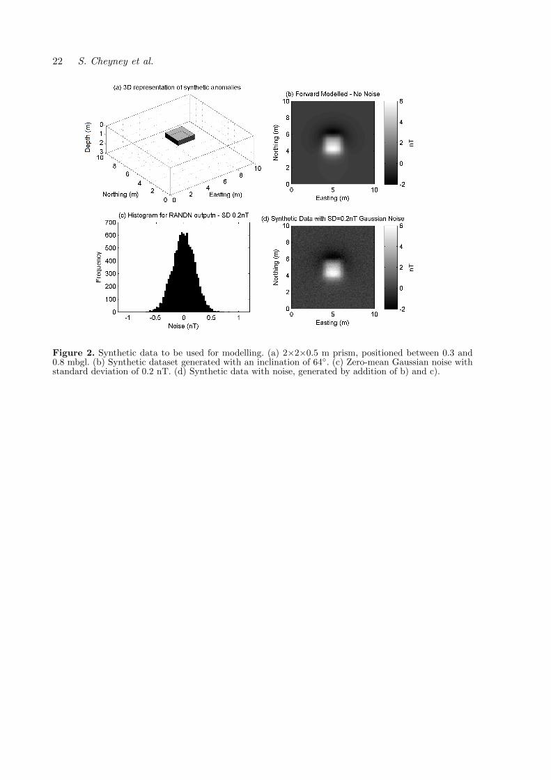
A synthetic prism 2×2×0.5 m, positioned between 0.3 and 0.8 meters below ground level

(mbgl) has been forward modelled with a susceptibility of 0.001 (SI) in an inducing field of

37.5 Am−1 with inclination of 64◦, at a survey height of 0.2 m (Fig. 2). The spatial sampling

of this dataset is 0.1×0.1 m. Zero-mean Gaussian noise with a standard deviation of 0.2 nT

has been added to produce the synthetic dataset. Although simplistic, these dimensions and

magnitude could be similar to what would be expected from an Anglo-Saxon Grubenhauser,

commonly classed as a Sunken Feature Building.

To demonstrate the effects of these peripheral cells the synthetic data has been modelled

twice. The first inversion is run using a mesh consisting of a central core of 0.5×0.5×0.1 m

cells to the lateral extents of the survey area, and with one additional 1 m and one 2 m wide

cell beyond the survey area, to account for any regional trend. The second inversion has been


performed on a mesh of only the central core cells which are limited to the lateral extents of the

survey area.

In each inversion the smallest model is found by applying αs = 1, and αx, αy, αz = 0 to the

objective function. As only a positive body is desired from the modelling in this case, positivity

has been constrained. Models of comparable data misfit have been derived, and the calculated

data can be seen in Fig. 3, for both the extended mesh, and the central core-only mesh inversion.

Comparison to Fig. 2d shows a good correlation between the observed and calculated data for

both scenarios.

The inverse model is shown for the extended mesh (Fig. 4a), and for the central-core mesh

(Fig. 4b). In both scenarios the lateral positions of the anomalous body has been reproduced

successfully, however the vertical extents differ. In Fig. 4a, the synthetic body has been recov-

ered as a significant anomaly from the very near surface to depths of around 2.5 mbgl, reaching

a maximum susceptibility of 0.0008 (SI) at depths around 1 to 1.5 mbgl. In Fig. 4b, the ver-

tical position of the synthetic body has been recovered more accurately, with an increase in

susceptibility towards 0.001 (SI), positioned between ∼0.3 and 0.8 mbgl as expected.

A key difference between the two models is the presence of anomalously high susceptibility

values in the 3 m wide outer cells that surround the central core cells in Fig. 4a. High values

are particularly noticeable towards the southern side of the mesh, and have peak amplitudes of

0.0004 (SI) increasing towards the base of the mesh. To illustrate the effect of these features,

the susceptibilities in the outer cells were isolated and forward modelled to see the impact on

the calculated dataset (Fig. 5).

It is shown that the outer cells have been used to create a regional trend across the area.

In this case, a negative magnetic field has been calculated for the southern-most observation

points. A gradient has been placed across the survey area from -0.45 nT in the south, to ∼0 nT

in the north. In this synthetic scenario there is no regional trend across the area, and therefore

all anomalies should be accounted for by susceptibilities within the main part of the mesh. The

effect of this negative trend across the survey area has resulted in higher susceptibility being

required from the main bodies, and hence could explain the deeper than expected extent of the

simulated archaeological bodies. The type of trend introduced by anomalous susceptibilities in

the outer cells varies depending on the magnetic inclination, but can still be observed, even in

a vertical inclination.

The approach of using an expanded mesh to account for regional trends has therefore nega-

tively impacted on the final result. Designing a mesh limited by the data extents has proven to

be a preferred method of recovering the synthetic bodies accurately. Where regional trends are

present in the dataset, it has proven to be advantageous to high-pass filter the data to remove

10 S. Cheyney et al.

the unwanted trends, prior to modelling with a mesh limited to the data extents. This approach

is contrary to methods typically employed in larger-scale mineral/exploration interpretations,

however has been demonstrated to be essential for accurate recovery of archaeological-scale

features. It is likely that the high-wavenumber content of archaeological anomalies makes the

separation of regional signal from the archaeological signal a simpler operation.

2.3 Apparent negative anomalies

The third point of focus of this study regards the occurrence of negative apparent susceptibility

contrasts. Once the processing of the data has reduced the total field measurement to a total

field anomaly dataset, these features are likely to show themselves as negative anomalies, and

when modelled, should produce negative apparent susceptibilities.

In order to produce a model that contains both positive and negative anomalies, the bound

constraints applied to the inversion can be adapted to allow the recovery of both positive and

negative apparent susceptibilities. The inverse problem is thus solved by minimising the objective

function (Equation 1) subject to:

m− <m < m+ (4)

where m is the susceptibility, and m− and m+ are a minimum and maximum susceptibility

assigned by the user. In all the above examples, positivity has been constrained as all the

recovered bodies were desired to consist of positive susceptibilities. This is achieved by setting

m− to zero, and m+ to a large value. Should negative apparent susceptibilities be desired in the

model, m− must be chosen as a negative value.

To test MAG3D’s ability to interpret negative susceptibilities, Fig. 2 has been duplicated to

consist of two identical prisms between 0.3 and 0.8 mbgl. The western prism has a susceptibility

of 0.001 (SI), and the eastern prism -0.001 (SI). As in Fig. 2, the positive prism has resulted in

a maximum total field response of ∼6 nT and the negative body has produced a response of the

same amplitude, but of opposite polarity. This negative anomaly could be representative of a

Roman building, constructed from a low magnetisation construction material such as rammed

chalk or flint, and typical of the type of anomalies seen later in the case study.

Modelling has been performed keeping the parameters the same as those used above, but this

time specifying maximum and minimum susceptibility limits of -0.05 and 0.05 (SI) respectively.

The mesh of 0.5×0.5×0.1 m cells, was limited to the data area of 16×10 m and extending down

to a depth of 4 mbgl. An optimum value for β has been identified by L-curve analysis (Lawson &

Hanson 1974; Hansen 1992). The L-curve is created to visualise the trade-off between the data


misfit and the model norm. The final result is chosen in the ‘knee’ of the curve, as this aids the

selection of a model where the coherent signal in the data has been modelled, yet leaving the

noise largely misfit. This ensures that the result includes all the structure required to fit the data,

without placing excessive, unrealistic structure into the model to fit noise in the observed data.

An east-west profile though the final inverse model at 4.25 mN is shown in Fig. 6. Both prisms

have been modelled by anomalous susceptibilities which slowly increase in amplitude from the

surface to a peak of ∼0.0006 (SI) for the positive body, and -0.0006 (SI) for the negative body,

at around 2 mbgl. Below this depth the susceptibility decreases, yet remains anomalous to the

base of the mesh at 4 mbgl. This has obviously resulted in modelled bodies with larger depth

extent than the 0.5 m thick prisms used to generate the observations.

Focussing on the positive prism, it can be seen that the modelled large positive body is

adjacent to lower amplitude negative bodies on either side. These negative apparent susceptibil-

ities are about -0.0001 to -0.0002 (SI). To illustrate the effect these negative features are having

on the data fit, all negative susceptibilities have been removed from the model. The remaining

positive susceptibilities have been forward modelled and the E-W profile is presented again in

Fig. 7. Without the negative susceptibilities on either side of the positive body, the calculated

data shows a much broader signal and does not produce a good fit to the data either side of the

prism location. The negative susceptibilities thus are placed into the model to create a shorter

wavelength feature in the calculated dataset, rather than placing the anomaly shallower, which

in this case would result in a better fit to the actual prism location. This shows the importance of

constraining polarity to force modelling of positive anomalies by purely positive susceptibilities,

and vice-versa.

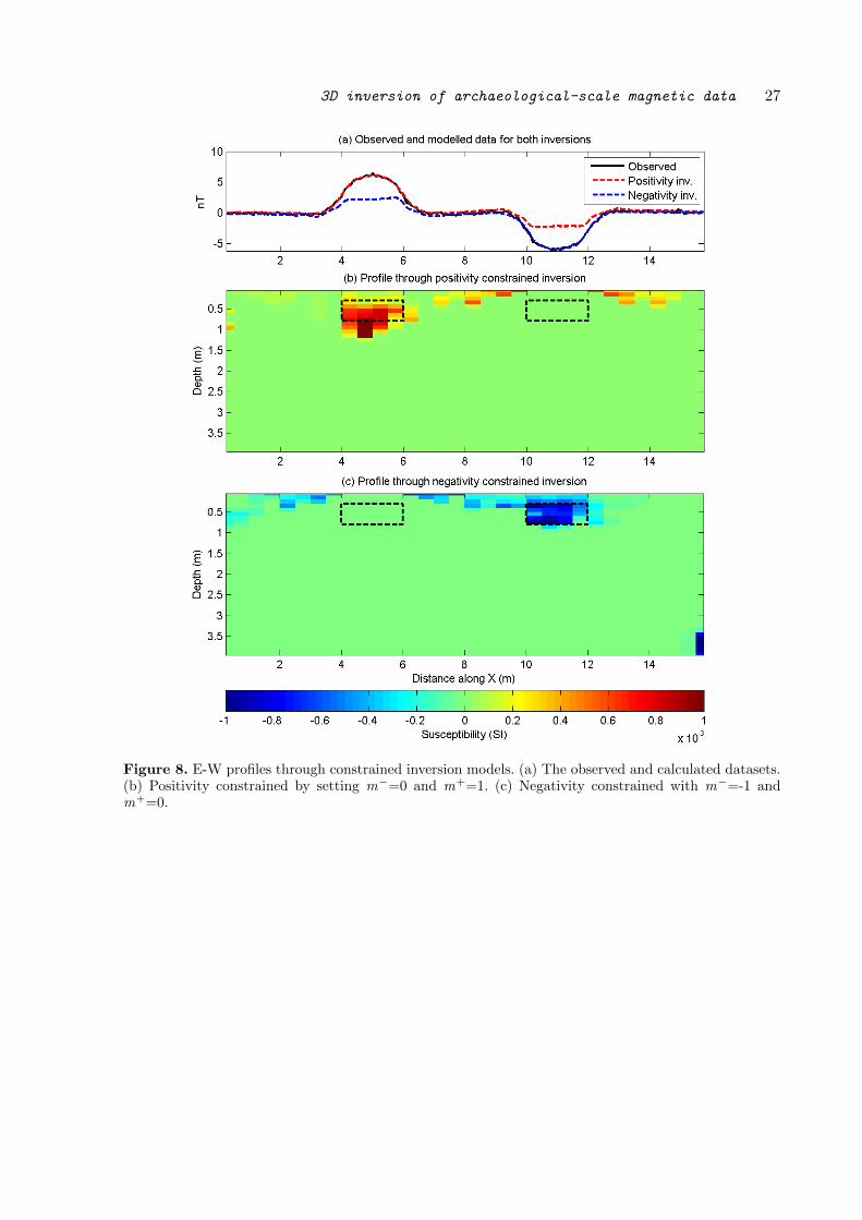
Placing a positivity constraint on the inversion will force the inversion to fit the anomalies

identified in the observations with positive susceptibility features in the model (Fig. 8b). A much

improved fit to the actual prism location can be seen for the positive prism as the inversion has

been forced to move the body shallower in order to create a good fit. Without allowing regional

trends or negative susceptibilities only a poor fit to the negative prism can be made. The same

procedure can be conducted for a negativity constrained inversion (Fig. 8c), and shows an

excellent fit to the negative prism, with a large data misfit in the area of the positive prism.

2.4 Constructing a reference model

As expected, the positivity model has provided a good fit to the positive prism, and failed to

fit the negative prism, where the model largely consists of zero susceptibilities. The negativity

constrained inversion has produced a good fit to the negative prism, and has zero susceptibilities

in the vicinity of the positive prism. Therefore for each cell within the mesh, a simple way to


create a reference model is to add the susceptibility recovered in the positivity model to the

value in the corresponding cell of the negativity model to produce a reference model. The model

norm, shown in Equation 3 penalises structure in the model dependant upon how far it deviates

from the reference model. Until now, all inverse models presented have been modelled using a

zero halfspace model, in order to recover models with the lowest susceptibilities required to fit

the data, and therefore recovering the ‘smallest’ model. It is possible to use prior knowledge to

generate a reference model and thus bias the inversion result, however in the absence of such

information the positivity and negativity constrained inversion results can be used. Using the

model generated by adding the positivity and negativity model as the reference model should

ensure that the structure of the final model produces a similar model to the reference and does

not revert towards the model seen in Fig. 6.

This method for creating a reference model is easily achieved and can be accomplished rapidly

once the initial constrained modelling has been run. It can however, be improved. Edge detection

allows the horizontal extents of anomalies to be accurately identified, and methods such as the

horizontal gradient magnitude, theta map and tilt angle can be adapted for use with archeo-

magnetic datasets (Cheyney et al. 2011). These techniques can be used to make informed choices

about where to pick and choose from the corresponding positivity and negativity constrained

models when creating a reference model.

Fig. 9 shows the edge detection process. Firstly the data are reduced to the pole (Fig. 9a), and

the pseudo-gravity transformation is applied (Fig. 9b). Then the horizontal gradient magnitude

of the pseudo-gravity dataset is calculated (Fig. 9c) and edges are defined as being located at

the peak amplitudes of the horizontal gradient magnitude. This allows the two bodies to be

defined by their lateral locations, and an indication is then made as to whether they relate to

positive or negative anomalies. This interpretation is shown in Fig. 9d.

Next, for the surface area that relates to an indicated positive anomaly in Fig. 9d, the

corresponding mesh cells directly below this point are taken from the positivity model, and

vice-versa from the negativity model. This results in a model that is populated immediately

below the anomaly areas, and is empty in all other cells (Fig. 10). This model can then be

used as a reference model for a subsequent inversion. A key advantage of using this approach

to constructing the reference model is that any spurious structure introduced as the initial con-

strained inversions attempt to fit anomalies of the opposite polarity, can be removed. This is

likely to degrade the data fit produced by the model (Fig. 10c), and hence the reference model

alone cannot be considered a solution, but a subsequent final inversion can be run with the

polarity constraints relaxed, therefore modifications required to fit the data are unconstrained

by polarity.


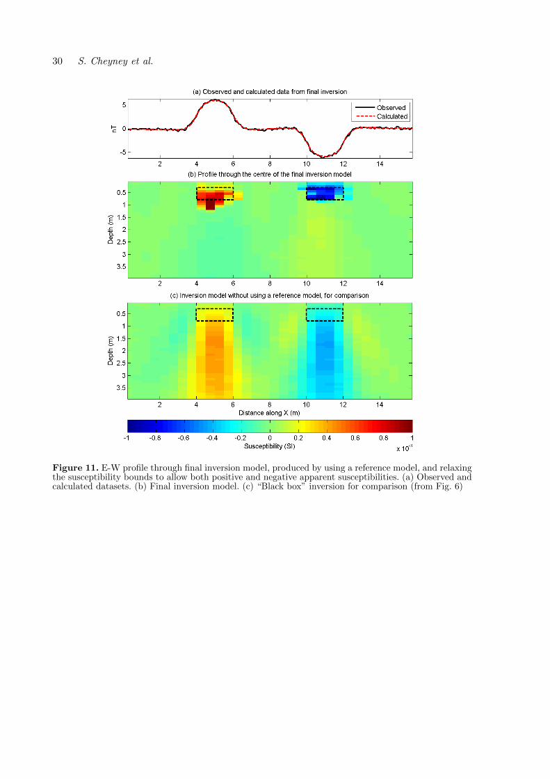
The dataset has been re-inverted with the addition of the reference model in place of a

zero-halfspace model in the objective function. The data fit, and an E-W profile through the

final model along 4.25 mN are presented in Figs 11a-b. The positive and negative prisms have

both been modelled well, with the negative prism almost entirely contained within the actual

prism volume, whereas the positive prism has been modelled ∼0.1-0.2 m too deep, as was the

case with the original inversion where the positivity constraint was applied. Thus, the addition

of the reference model, generated from initially constrained inversions has significantly improved

the fit to the synthetic bodies when compared to the original inversion, which is shown again in

Fig. 11c for comparison.

3 Case study

The methodology developed on synthetic data is demonstrated on a case study from Silchester,

Hampshire, UK. The site is known to have been an Iron Age settlement, and contains the remains

of the Roman town of Calleva Atrebatum (Fulford 2002). A survey within the town walls was

conducted in June 2009 by English Heritage. The data were collected with a 0.125×0.5 m

resolution, measuring the total field using caesium vapour magnetometers. The data are shown

in Fig. 12a, where an abundance of responses indicative of Roman activity at the site can be

seen. The most notable features are the linear grid pattern of roads, the Forum Basilica towards

the north-east of the survey area, and the circular looking feature towards the south-east of the

survey area, which has been used here as the focus of the case study. The subset is approximately

40×40 m, and is believed to be a Romano-Celtic temple positioned within Insula VII (Fig. 12b).

The temple has previously been excavated in 1870 and 1892 (Thomson 1924).

The results of the latter excavation are described by Fox & Hope (1894). The total diameter

of the temple was found to be around 19.81 m, consisting of two concentric rings. The foundations

of the outer ring are described as consisting of a slaty stone, which shows the 16-sided polygonal

shape. The foundations are 0.91 m thick, on top of which is found evidence for a wall of flint

rubble masonry. This wall is 0.74 m wide, and also shows the polygonal shape, which each section

measuring 3.86 m. The angles are strengthened inside and out by blocks of ironstone, which has

also been used as bonds to the flint rubble masonry that make up the walls.

The foundations of the inner ring abandons the polygonal shape, and is circular, 1.22 m

wide, once again made of slaty stone. Above this stood a wall, 0.76 m thick, which has the

16-sided polygonal shape on the outer side, yet is circular on the inner side. The length of each

outer face is 2.44 m. At no point during the excavation was either wall found to be greater than

0.48 m above the footings.

The first step in interpreting the data, is to identify the lateral edge positions of the anoma-


lies. The pseudogravity transformation has been applied, and then the horizontal gradient mag-

nitude derived and shown in Fig. 12c. The location of the peaks have been interpreted manually

to produce an outline of suspected buried bodies (Fig. 12d). In total 22 anomalous zones have

been identified.

3.1 Initial inversions

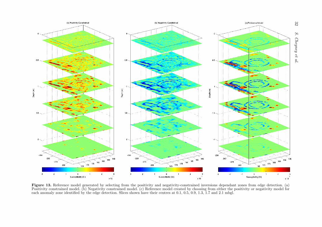
During the first run of the inversion, a positivity constraint is placed on the recovered suscep-

tibilities to ensure that the positive anomalies in the model are modelled by a single positive

susceptibility contrast (Fig. 13a). For the second run a negativity constraint is imposed, so that

any negative features are modelled by a negative apparent susceptibility contrast rather than a

combination of positive and negative (Fig. 13b). For each zone identified in the edge detection

a decision is made as to whether it represents positive or negative apparent susceptibility con-

trasts, bearing in mind the dipolar nature of magnetic fields. A reference model is formed by

placing the susceptibilities from the relevant model into the reference model for the cells beneath

each zone (Fig. 13c). All other parts of the reference model are set to a zero susceptibility.

3.2 Inverse model

In order to obtain the final model for the dataset, a third run of the inverse procedure is required,

this time relaxing the constraints on the recovered susceptibilities to −0.5 ≤ m ≤ 0.5. The

reference model shown in Fig. 13c is used in the objective function in place of a zero-halfspace

model.

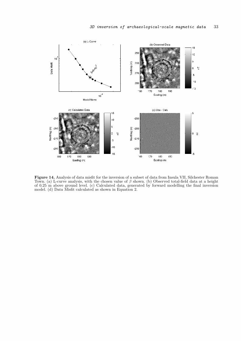
An optimum value of β was chosen by analysis of the L-curve (Fig. 14a), with the β repre-

senting the solution in the ‘knee’ of the curve chosen. A good fit between the observed (Fig. 14b)

and calculated data (Fig. 14c) has been achieved, with only isolated peaks present in the data

misfit, representing point sources that cannot be accurately modelled with the resolution of the

mesh chosen (Fig. 14d).

To demonstrate the difference in the final interpretation, slices from an unconstrained inver-

sion, using default parameters (Fig. 15a) are compared to slices from the final inversion, using

the adapted methodology discussed above (Fig. 15b). The temple is the most striking feature

in the dataset represented by the double circular pattern towards the centre of the area. It is

particularly noticeable that the default inversion has recovered significantly lower susceptibili-

ties, with a much greater depth extent. In the lower slices of Fig. 15a, it can be observed that

the temple is represented by both a negative susceptibility (as would be expected), and also a

positive susceptibility either side of the temple walls. This is the same effect that was observed

during the synthetic testing.


Fig. 16a, shows more of the upper slices of the model, with centres at 0.1, 0.3, 0.5, 0.7, 1.1,

1.3, 1.7 and 1.9 mbgl. The temple is visible in the slices immediately below the ground surface,

however a notable increase in the susceptibility contrast is present at 0.5 mbgl, and is visible in

depth slices to 2 mbgl. The susceptibility contrast between the surrounding soil and the temple

is around -0.002 (SI).

3.3 Comparison to Ground Penetrating Radar

As the excavations over the Romano-Celtic temple at Silchester were conducted in the late 19th

century, only limited information is available. The surviving records show a plan view of the

buried walls with no sections to obtain more useful depth information. The site at Silchester has

however, been surveyed several times with different geophysical methods. It is particularly useful

to compare the results of the 3D magnetic modelling to datasets from a ground penetrating radar

(GPR) survey, where the presentation of the final model with depth slices is a commonplace for

the interpretation of the data.

Here, two GPR datasets are shown, both collected by English Heritage. The June 2009

dataset (Linford et al. 2010), shown in Fig. 16b was collected at the same time as the magnetic

survey interpreted above. Data collection was with a 3D-Radar GeoScope stepped-frequency

continuous wave GPR. The system works by transmitting a continuous-wave signal over a series

of discrete frequency steps ranging between 100 MHz and 1.2 GHz at each recording station.

A horizontal resolution of 0.075×0.075 m was achieved by towing the GPR behind a vehicle. A

more traditional GPR survey was conducted in March 2000 using a Pulse Ekko 1000 impulse

GPR system with a 450 MHz antenna (Linford 2001). The sample interval derived with this

system was 0.05×0.5 m and selected slices are shown in Fig. 16c. The GPR data are presented

following minimal data processing including background subtraction and the application of a

suitable gain function to enhance later reflections in the profiles. The summary time slices shown

here have been integrated vertically over a 4 ns two-way travel time representing a physical depth

slice of ∼0.15 m.

The higher resolution of the GeoScope dataset is particularly notable, yet the position and

extents of the temple are shown in all three datasets. The temple foundations are also visible

in the shallowest slices from the GeoScope dataset (0.1 and 0.3 mbgl), suggesting that the

foundations are either very shallow, or that there has been significant disturbances to the ground

immediately above the foundations due to the excavation work. The weaker response in the

upper slices may also be indicative of a response to the remains of the walls, built on top of the

foundations, and thinner than the foundations they sit on, as described by Fox & Hope (1894).

Below this, all three methods show a strong response to the temple foundations to a depth


of around 1.7 mbgl, where the amplitude of the magnetic and GeoScope GPR anomaly suddenly

decreases, and the signal to noise ratio of the PulseEkko GPR causes any response to be obscured

by noise.

4 Conclusions

3D inversion has been conducted on synthetic and real archaeological datasets using MAG3D de-

veloped by the University of British Columbia, Geophysical Inversion Facility (UBC-GIF). This

code has been primarily applied to aero-magnetic surveys of a regional-scale, and some adapta-

tions to the procedures have been required to obtain confidence in the results from archaeological

magnetic data.

Here it has been demonstrated that the standard mesh design of MAG3D featuring a cen-

tral core consisting of small cells in the volume of interest, with larger cells surrounding this

outside the limits of the observation points, needs to be modified to achieve satisfactory models

of archaeological datasets. The standard approach has not been very successful at recovering

archaeological-type anomalies, as the outer cells, poorly constrained by nearby data, have been

shown to account for significant trends across the survey area, even for datasets where no regional

trend is present. This has a dramatic effect on the ability to accurately recover the archaeological

features. It is therefore essential that any regional trends that exist in the dataset are removed

prior to inversion, and that only the core central cells of the mesh are used in the inversion

to ensure that all features in the dataset are accounted for in the mesh immediately below the

observation points.

Archaeological bodies buried within susceptible soils are often represented by both positive

and negative anomalies with respect to the background level of the magnetic field. Where both

positive and negative apparent susceptibility contrasts are suspected it has been demonstrated

here that to accurately recover the subsurface anomalies a multi-stage procedure is required.

Initially, two inversions must be performed, one with a positivity constraint and one with a

negativity constraint. Using the output from edge-detection techniques, a reference model is then

created using the appropriate part of the positivity and negativity-constrained models based on

the polarity of the observations (keeping in mind the dipolar nature of magnetic fields). The

inversion can then be re-run for a final time, with the susceptibility constraints relaxed to allow

both positive and negative values, and with the reference model built into the objective function

to ensure the model retains the structure as close as possible to the preliminary inversion results.

The inversion of magnetic data does not produce a unique solution, and it is common prac-

tice to attempt to produce a single solution on the basis that the model should be as simple or

smooth as possible whilst fitting the data to a suitable degree. This procedure is employed as


it will reduce the temptation to over-interpret the data. Synthetic testing illustrates that when

this approach is taken (without a reference model, and constraints on the modelled anomalies),

the inversion procedure is unable to reproduce the shallow causative anomalies typical of ar-

chaeological studies. In contrast, following the multi-stage procedure gives a good recovery of

the synthetic features (Fig. 11). As this is moving away from the simplest model approach it

could therefore, potentially lead to an over-interpretation of the results. It may be possible that

any spurious structure introduced to fit bodies of opposite polarities in the initial inversion runs,

cannot be identified and removed prior to the construction of the reference model. This could

be the case when anomalies of opposite polarity are closely adjacent or overlapping, or features

are dipping at shallow angles that cannot be accounted for by the edge detection routines. For

archaeological purposes these effects are likely to be somewhat mitigated by the limited range

of influence that shallowly buried, weakly magnetised bodies have.

The case study of Silchester has allowed the approach to be tested with real data. Further-

more, the magnetic model produced is comparable with results from ground penetrating radar,

and variations in the magnetic susceptibility show broad agreement with the structure recovered

from the dielectric properties. Keeping in mind the potential of over-interpretation, the results

obtained by the multi-stage procedure are eminently more useful than the unconstrained, yet

‘simple’ models.

This added level of interpretation of very near-surface magnetic data therefore allows the

physical properties of the causative bodies to be analysed as opposed to the resultant anoma-

lies produced by them. It can be used to further aid interpretation regarding the 3-dimensional

position and material make-up of the subsurface, and move beyond simple visual pattern recog-

nition from a plan of anomalies. Subsequent decisions as to whether to build on top of the buried

features, perform more detailed surveys or commence excavation can be made with added con-

fidence.

ACKNOWLEDGMENTS

This work was funded by NERC doctoral training grant NE/G523798/1, and CASE sponsored by

Geomatrix Earth Science Ltd. We would like to thank English Heritage (now Historic England)

for all their assistance and allowing the use of the data, and the University of British Columbia’s

Geophysical Inversion Facility for the MAG3D software.


REFERENCES

Aspinall, A., Gaffney, C., & Schmidt, A., 2008. Magnetometry for Archaeologists, AltaMira Press,

U.S.A., 1st edn.

Cella, F. & Fedi, M., 2012. Inversion of potential field data using the structural index as weighting

function rate decay, Geophysical Prospecting , 60, 313–336.

Cheyney, S., Hill, I., & Linford, N., 2011. Advantages to using the pseudogravity transformation to aid

edge detection of total field archaeomagnetic datasets, Archaeological Prospection, 18, 81–93.

Cordell, L. & Grauch, V. J. S., 1985. Mapping basement magnetization zones from aeromagnetic data

in the San Juan Basin, New Mexico., pp. 181–197, The utility of regional gravity and magnetic maps,

Society of Exploration Geophysicists, Tulsa, USA, 1st edn.

Dittmer, J. K. & Szymanski, J. E., 1995. The stochastic inversion of magnetics and resistivity data

using the simulated annealing algorithm, Geophysical Prospecting , 43(3), 397–416.

Eder-Hinterleitner, A., Neubauer, W., & Melichar, P., 1995. Reconstruction of archaeological structures

using magnetic prospection, pp. 131–137, Interfacing the past: Computer Applications and Quantitative

Methods in Archaeology, Analecta Praehistorica Leidensia 28, University of Leiden.

Fassbinder, J., Stanjek, H., & Vali, H., 1990. Occurrence of magnetic bacteria in soil, Nature, 343(6254),

161–163.

Fox, G. E. & Hope, W. H. S., 1894. Excavations on the site of the roman city at silchester, hants, in

1893, Archaeologia (Second Series), 54, 199–238.

Fulford, M., 2002. A Guide to Silchester: The Roman Town of Calleva Atrebatum, Calleva Trust, Stroud,

U.K., 2nd edn.

Graham, I. & Scollar, I., 1976. Limitations on magnetic prospection in archaeology imposed by soil

properties, Archaeo-Physika, 6, 1–125.

Hansen, P. C., 1992. Analysis of discrete ill-posed problems by means of the l-curve, SIAM Review ,

34(4), 561–580.

Herwanger, J., Maurer, H., Green, A. G., & Leckebusch, J., 2000. 3-d inversions of magnetic gradiometer

data in archaeological prospecting; possibilities and limitations, Geophysics, 65(3), 849–860.

Lawson, C. L. & Hanson, R. J., 1974. Solving Least Squares Problems, Prentice-Hall Inc, New Jersey,

USA, 1st edn.

Le Borgne, E., 1955. Susceptibilit magntique anormale du sol superficiel, Annales de Geophysique, 11,

399–419.

Lelievre, P. G. & Oldenburg, D. W., 2006. Magnetic forward modelling and inversion for high suscep-

tibility, Geophysical Journal International , 166(1), 76–90.

Li, Y. & Oldenburg, D. W., 1996. 3-d inversion of magnetic data, Geophysics, 61(2), 394–408.

Li, Y. G. & Oldenburg, D. W., 2003. Fast inversion of large-scale magnetic data using wavelet transforms

and a logarithmic barrier method, Geophysical Journal International , 152(2), 251–265.

Linford, N., 2001. Silchester roman town, hampshire; report on ground penetrating radar survey, march

2000, Tech. Rep. Centre for Archaeology Report Number 9/2001, English Heritage.


Linford, N., 2004. Magnetic ghosts: Mineral magnetic measurements on roman and anglo-saxon graves,

Archaeological Prospection, 11, 167–180.

Linford, N., 2006. The application of geophysical methods to archaeological prospection, Reports On

Progress In Physics, 69(7), 2205–2257.

Linford, N., Linford, P., Martin, L., & Payne, A., 2010. Stepped frequency ground-penetrating radar

survey with a mulit-element array antenna: Results from field application on archaeological sites.,

Archaeological Prospection, 17, 187–193.

Maher, B. A. & Taylor, R. M., 1988. Formation of ultrafine-grained magnetite in soils, Nature, 336,

368–371.

Miller, H. G. & Singh, V., 1994. Potential field tilt; a new concept for location of potential field sources,

Journal of Applied Geophysics, 32(2-3), 213–217.

Nabighian, M. N., 1972. The analytic signal of two-dimensional magnetic bodies with polygonal cross-

section; its properties and use for automated anomaly interpretation, Geophysics, 37(3), 507–517.

Pilkington, M., 1997. 3-d magnetic imaging using conjugate gradients, Geophysics, 62(4), 1132–1142.

Piro, S., Sambuelli, L., Godio, A., & Taormina, R., 2007. Beyond image analysis in processing archaeo-

magnetic geophysical data: case studies of chamber tombs with dromos, Near Surface Geophysics, 5(6),

405–414.

Powell, D. W., 1967. Fitting observed profiles to a magnetized dyke or fault-step model, Geophysical

Prospecting , 15, 208–220.

Ravat, D., Pignatelli, A., Nicolosi, I., & Chiappini, M., 2007. A study of spectral methods of estimating

the depth to the bottom of magnetic sources from near-surface magnetic anomaly data, Geophysical

Journal International , 169(2), 421–434.

Reid, A. B., Allsop, J. M., Granser, H., Millett, A. J., & Somerton, I. W., 1990. Magnetic interpretation

in 3 dimensions using euler deconvolution, Geophysics, 55(1), 80–91.

Saracco, G., Moreau, F., Math, P.-E., Hermitte, D., & Michel, J.-M., 2007. Multiscale tomography of

buried magnetic structures: its use in the localization and characterization of archaeological structures,

Geophysical Journal International , 171(1), 87–103.

Sheriff, S. D., MacDonald, D., & Dick, D., 2010. Decorrugation, edge detection, and modelling of total

field magnetic observations from a historic town site, yellowstone national park, usa, Archaeological

Prospection, 17(1), 49–60.

Smith, R. S., Thurston, J. B., Dai, T.-F., & MacLeod, I. N., 1998. ispi (super tm) ; the improved

source parameter imaging method, Geophysical Prospecting , 46(2), 141–151, Format: illus. incl. 1

table; References: 17.

Thomson, J. C., 1924. A Great Free City: The Book of Silchester , Simpkin, Marshall, Hamilton, Kent

& Co. Ltd, London, volume 1 edn.

Thurston, J. B. & Smith, R. S., 1997. Automatic conversion of magnetic data to depth, dip, and

susceptibility contrast using the spi (tm) method, Geophysics, 62(3), 807–813.

UBC-GIF, 2005. Mag3d: A program library for forward modelling and inversion of magnetic data over

3d structures. version 4.0.


Wijns, C., Perez, C., & Kowalczyk, P., 2005. Theta map; edge detection in magnetic data, Geophysics,

70(4), L39–L43.

Williams, N. C., 2008. Geologically-constrained UBC-GIF gravity and magnetic inversions with exam-

ples from the Agnew-Wiluna greenstone belt, Western Australia, Ph.D. thesis, University of British

Columbia.


Figure 1. Optimum depth weighting parameters to the kernel response. Depth weighting parameters forvarious values of γ, for a 4m deep mesh of cells 0.5×0.5×0.1 m. The optimum parameters for values ofγ = 1, 2 and 3 are shown as well as an optimum where γ and z0 were allowed to vary. Solutions derivedby Nelder-Mead simplex direct search.


Figure 2. Synthetic data to be used for modelling. (a) 2×2×0.5 m prism, positioned between 0.3 and0.8 mbgl. (b) Synthetic dataset generated with an inclination of 64◦. (c) Zero-mean Gaussian noise withstandard deviation of 0.2 nT. (d) Synthetic data with noise, generated by addition of b) and c).


Figure 3. Calculated data from the inversion of the synthetic body in Fig. 2. (a) Using a mesh withpadding cells around the horizontal extents. (b) Without padding cells, using just the central ‘core’ ofthe mesh. The data misfits obtained for the two inversions are approximately the same.


Figure 4. Final inversion model for the synthetic body presented in Fig. 2. (a) Inversion with mesh thatincludes padding cells surrounding the centre mesh. (b) Inversion using mesh of just the central cells.Slices shown have their centres at 0.05, 0.35, 0.65, 0.95, 1.25, 1.55, 1.85 and 2.15 mbgl. The syntheticprism is shown to have much larger vertical extents in a), and there is a higher susceptibility placed intothe poorly constrained padding cells.


Figure 5. Forward modelling of the anomalous susceptibilities placed within the peripheral cells of theinversion shown in Fig. 4a. The outer cells have been used to produce a gradient across the survey areafrom -0.45 nT in the south to 0 nT in the north.

Figure 6. East-west profile along 4.25 mN, through an inversion model with both positive and negativesynthetic anomalies. The modelling has produced a good fit to the observations by creating a negative-positive-negative pattern for the positive anomaly, and vice-versa for the negative anomaly.


Figure 7. Forward modelling just using the positive susceptibilities from Fig. 6. It is demonstrated thatthe positive susceptibilities are not sufficient to fit the observed dataset (around 3.5 m and 6.5 m alongline), and the negative susceptibilities that make up the negative-positive-negative pattern observed inFig. 6 are essential for providing a good fit.


Figure 8. E-W profiles through constrained inversion models. (a) The observed and calculated datasets.(b) Positivity constrained by setting m−=0 and m+=1. (c) Negativity constrained with m−=-1 andm+=0.


Figure 9. Edge detection of dataset consisting of a positive and negative synthetic anomaly (a) Firstlythe dataset it reduced to the pole. (b) Pseudo-gravity dataset (c) Horizontal gradient magnitude ofpseudo-gravity. (d) Interpretation of c) with indication of polarity of amplitude made from a).


Figure 10. (a) The observed and forward modelled datasets along an E-W profile through the referencemodel along 4.25 mN. (b) The reference model along the same E-W profile. (c) The difference betweenthe observed and forward modelled data. Note that the reference model does not produce a satisfactoryfit to the data.


Figure 11. E-W profile through final inversion model, produced by using a reference model, and relaxingthe susceptibility bounds to allow both positive and negative apparent susceptibilities. (a) Observed andcalculated datasets. (b) Final inversion model. (c) “Black box” inversion for comparison (from Fig. 6)


Figure 12. Insula VII, Silchester Roman Town. (a) Full extent of collected total field dataset. (b)Subset of data over the Romano-Celtic temple in Insula VII (c) Horizontal gradient magnitude of thepseudogravity of b) (d) Interpretation of the edge locations based c).

32

S.Cheyn

eyet

al.

Figure 13. Reference model generated by selecting from the positivity and negativity-constrained inversions dependant zones from edge detection. (a)Positivity constrained model. (b) Negativity constrained model. (c) Reference model created by choosing from either the positivity or negativity model foreach anomaly zone identified by the edge detection. Slices shown have their centres at 0.1, 0.5, 0.9, 1.3, 1.7 and 2.1 mbgl.


Figure 14. Analysis of data misfit for the inversion of a subset of data from Insula VII, Silchester RomanTown. (a) L-curve analysis, with the chosen value of β shown. (b) Observed total-field data at a heightof 0.25 m above ground level. (c) Calculated data, generated by forward modelling the final inversionmodel. (d) Data Misfit calculated as shown in Equation 2.


Figure 15. Comparison between (a) An unconstrained inversion with default parameters, and (b) Thefinal inversion model.

3Dinversionofarchaeological-scalemagneticdata

35

Figure 16. Comparison between magnetic inversion model and GPR depth slices. (a) Magnetic inversion with slices shown at 0.1, 0.3, 0.5, 0.7, 1.1, 1.3,1.7 and 1.9 mbgl (b) GeoScope 100-1200 MHz stepped frequency (from Linford et al. (2010)). (c) PulseEkko 1000, 450 MHz antenna (from Linford (2001)).As expected the low magnetic susceptibility walls equate to positive high amplitude GPR anomalies.

Documents

Successful adaptation to 3D inversion methodologies for ... · Successful adaptation to 3D inversion methodologies for archaeological-scale, ... English Heritage, ... The rst term