Suction Caissons: Seafloor Characterization for Deepwater

Suction Caissons: Seafloor Characterization for Deepwater Fo undation Systems

By

Shadi S. Najjar, Graduate Research Assistant Robert B. Gilbert, P.E., Ph.D.

Geotechnical Engineering Center

Civil Engineering Department The University of Texas at Austin

Final Report on the Suction Caissons: Seafloor Characterization for Deepwater Foundation Systems Study

for the Project Suction Caissons and Vertically Loaded Anchors

Prepared for the Minerals Management Service

Under the MMS/OTRC Cooperative Research Agreement 1435-01-99-CA-31003

Task Order 16169 1435-01-04-CA-35515

Task Order 35980 MMS Project Number 362

and

OTRC Industry Consortium

June 2006

OTRC Library Number:6/06B171

“The views and conclusions contained in this document are those of the authors and

should not be interpreted as representing the opinions or policies of the U.S. Government. Mention of trade names or commercial products does not constitute

their endorsement by the U. S. Government”.

For more information contact:

Offshore Technology Research Center Texas A&M University

1200 Mariner Drive College Station, Texas 77845-3400

(979) 845-6000

or

Offshore Technology Research Center The University of Texas at Austin

1 University Station C3700 Austin, Texas 78712-0318

(512) 471-6989

A National Science Foundation Graduated Engineering Research Center

PREFACE The project Suction Caissons and Vertically Loaded Anchors was conducted as series of inter-related studies. The individual studies are as follows:

• Suction Caissons & Vertically Loaded Anchors: Design Analysis Methods by Charles Aubeny and Don Murff, Principal Investigators

• Suction Caissons: Model Tests by Roy Olson, Alan Rauch and Robert Gilbert, Principal Investigators

• Suction Caissons: Seafloor Characterization for Deepwater Foundation Systems by Robert Gilbert Principal Investigator

• Suction Caissons: Finite Element Modeling by John Tassoulas Principal Investigator

This report summarizes the results of the Suction Caissons: Seafloor Characterization for Deepwater Foundation Systems, study.

i

TABLE OF CONTENTS PREFACE........................................................................................................................... ii TABLE OF CONTENTS.................................................................................................... ii LIST OF TABLES............................................................................................................. iii LIST OF FIGURES ........................................................................................................... iii Introduction......................................................................................................................... 1 Spatial Variability in Suction Caisson Design Parameters ................................................. 2 Calibration of Suction Caisson Design Method.................................................................. 8

Capacity for Lateral and Inclined Loading ................................................................... 17 Lower-Bound Capacity................................................................................................. 17

Reliability-Based Design of Suction Caissons ................................................................. 20 Bias and C.o.v. Values for Deepwater Mooring Systems............................................. 22

Foundation Load ....................................................................................................... 22 Foundation Capacity ................................................................................................. 23 Median Factor of Safety, Total c.o.v. and Reliability............................................... 23

Lower-Bound Foundation Capacity.............................................................................. 25 Target Reliability .......................................................................................................... 28 Reliability-Based Design Considerations ..................................................................... 30

Adjusted Resistance Factor for Lower-Bound Capacity .......................................... 30 Added Design Checking Equation for Lower-Bound Capacity ............................... 32

Value of Site Characterization and Installation Data.................................................... 33 Summary ........................................................................................................................... 34 References......................................................................................................................... 36 Appendix A....................................................................................................................... 38 Description of Geotechnical Database Design ................................................................. 38

Database Features ......................................................................................................... 38 Tables—Data Storage and Entry .............................................................................. 38 Queries—Data Manipulation .................................................................................... 39 Forms—Automation ................................................................................................. 40 Modules—Programming Forms ............................................................................... 41

Database Structure ........................................................................................................ 42 Data Tables ............................................................................................................... 42 Boring Information ................................................................................................... 44 Index Properties ........................................................................................................ 44 Laboratory Engineering Properties ........................................................................... 44 Field Engineering Properties..................................................................................... 46 Design Information ................................................................................................... 47 Supplemental Information ........................................................................................ 47 Queries ...................................................................................................................... 48 Forms ........................................................................................................................ 48

Abbreviations................................................................................................................ 49 Modules..................................................................................................................... 49

ii

LIST OF TABLES Table 1. Summary statistics for spatial variability in total axial uplift capacity................ 3 Table 2. Statistics relating to maximum lateral capacity. .................................................. 4 Table 3. Comparison of total side friction for 25 simulated soil profiles. .......................... 7 Table 4. Comparison of net end bearing for 25 simulated soil profile.s............................. 7 Table 5. Variability in total capacity for 25 simulated soil profiles. .................................. 7 Table 6. Database of pullout tests on suction caissons (general description). .................. 10 Table 7. Database of pullout tests on suction caissons (soil properties and measured loads)................................................................................................................................. 11 Table 8. Biases and uncertainties in model for suction caissons (α=1, N=9). ................. 15 Table 9. Calibration of α and N (corrected undrained shear strength and excluding tests with setup = 0). ................................................................................................................. 16 Table 10. Bias and c.o.v. values for foundation in study spar. ......................................... 22 Figure 15. Reliability for study spar foundations versus design factor of safety (20-year design life). ....................................................................................................................... 29 Table A.1. Summary of Database Tables ........................................................................ 43 Table A.2. Summary of Database Queries....................................................................... 48 Table A.3. Tables and their Associated Forms ................................................................ 49

LIST OF FIGURES Figure 1. Example of spatial variability in suction caisson capacity across Gulf of Mexico deepwater boring sites......................................................................................................... 3 Figure 2. Schematic of generic suction caisson and driven pile. ........................................ 5 Figure 3. Generic soil profile. ............................................................................................. 6 Figure 4. Example of simulated strength profile. ............................................................... 6 Figure 5. Comparison between measured and predicted capacities for 25 suction caissons (uncorrected shear strength, α = 1, N = 9)........................................................................ 12 Figure 6. Comparison between measured and predicted capacities for 25 suction caissons (corrected undrained shear strength for direct simple shear, α = 1, N = 9). ..................... 14 Figure 7. Comparison between measured and predicted components of suction caisson capacity under inclined loading (El-Sherbiny 2005). ....................................................... 17 Figure 8. Evidence of Lower-Bound Capacity for 25 Suction Caissons .......................... 19 Figure 9. Results from a conventional reliability analysis on a pile in a typical jacket platform............................................................................................................................. 21 Figure 10. Results from a conventional reliability analysis on study spar foundations. .. 24 Figure 11. Mixed probability distribution for modeling suction caisson capacity. .......... 25 Figure 12. Effect of lower-bound capacity on reliability index........................................ 26 (c.o.v.Load = 0.15, c.o.v.Capacity = 0.3)................................................................................. 26 Figure 13. Variation of the required median factor of safety with the lower-bound capacity (c.o.v.Load = 0.15, c.o.v.Capacity = 0.3). ................................................................. 27 Figure 14. Effect of lower-bound capacity on probability of failure (study spar in 2,000-m water depth). ..................................................................................................................... 28

iii

Figure 16. Variation of the increase in the nominal resistance factor with the lower-bound capacity (c.o.v.Load = �Q = 0.15)....................................................................................... 31 Figure 17. Variation of the lower-bound resistance factor to account for a lower-bound capacity (c.o.v.Load = �Q = 0.15)....................................................................................... 33 Fig. A.1. A table in the database...................................................................................... 38 Fig. A.2. A query in Design View. A query viewed in Datasheet View looks like a table............................................................................................................................................ 39 Fig. A.3. Data from the Query is pasted into Excel to be plotted and analyzed.............. 40 Fig. A.4. An image form and a record in Form View...................................................... 41

iv

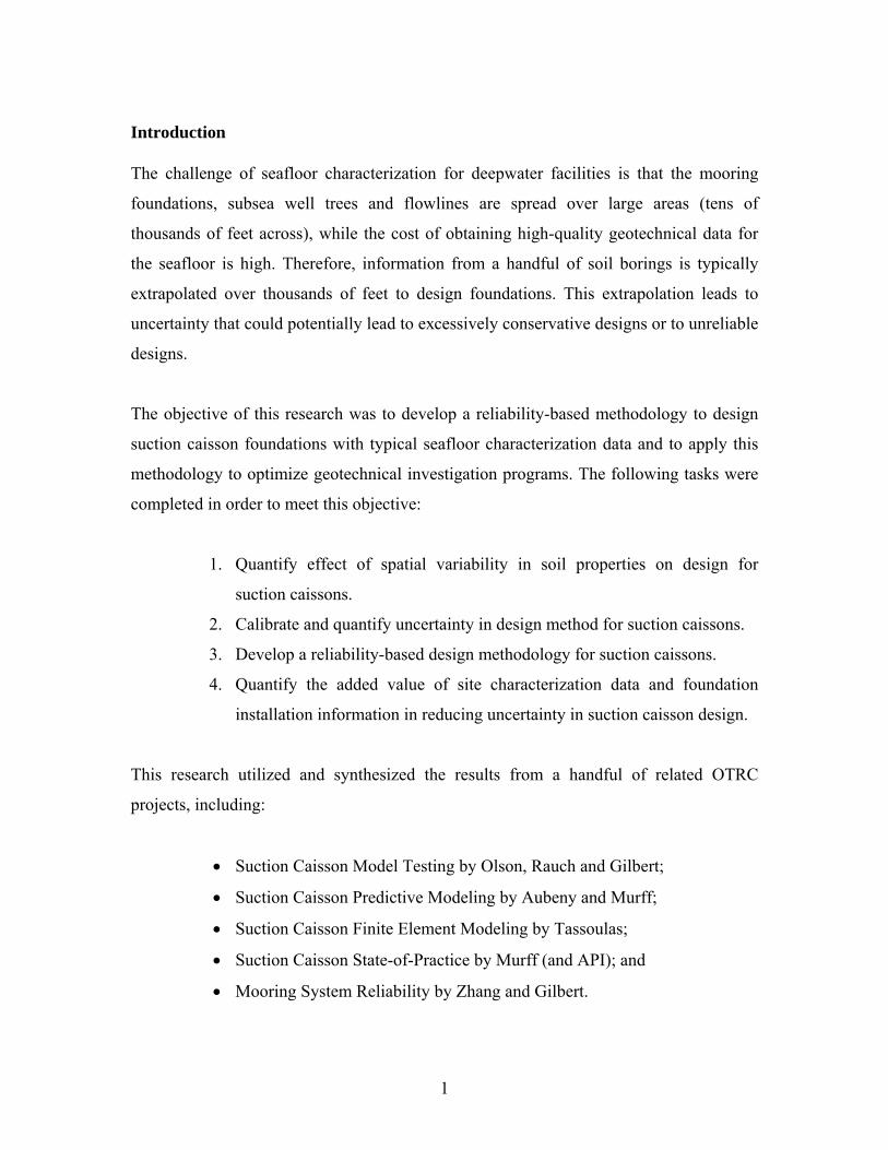
Introduction The challenge of seafloor characterization for deepwater facilities is that the mooring

foundations, subsea well trees and flowlines are spread over large areas (tens of

thousands of feet across), while the cost of obtaining high-quality geotechnical data for

the seafloor is high. Therefore, information from a handful of soil borings is typically

extrapolated over thousands of feet to design foundations. This extrapolation leads to

uncertainty that could potentially lead to excessively conservative designs or to unreliable

designs.

The objective of this research was to develop a reliability-based methodology to design

suction caisson foundations with typical seafloor characterization data and to apply this

methodology to optimize geotechnical investigation programs. The following tasks were

completed in order to meet this objective:

1. Quantify effect of spatial variability in soil properties on design for

suction caissons.

2. Calibrate and quantify uncertainty in design method for suction caissons.

3. Develop a reliability-based design methodology for suction caissons.

4. Quantify the added value of site characterization data and foundation

installation information in reducing uncertainty in suction caisson design.

This research utilized and synthesized the results from a handful of related OTRC

projects, including:

• Suction Caisson Model Testing by Olson, Rauch and Gilbert;

• Suction Caisson Predictive Modeling by Aubeny and Murff;

• Suction Caisson Finite Element Modeling by Tassoulas;

• Suction Caisson State-of-Practice by Murff (and API); and

• Mooring System Reliability by Zhang and Gilbert.

1

Spatial Variability in Suction Caisson Design Parameters

An important issue in site characterization for suction caissons is the spatial

variability in geotechnical properties. This variability leads to uncertainty in extrapolating

information from boring locations to the actual location of the foundation elements.

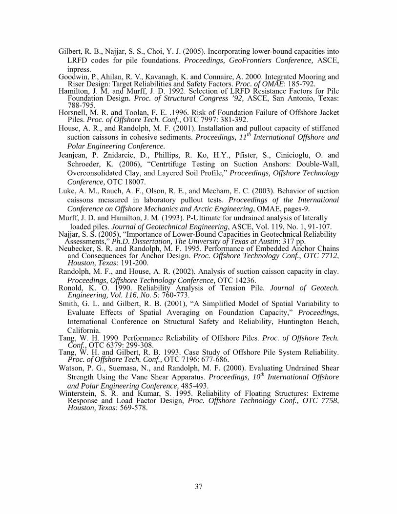
Proprietary site investigation and design information was compiled and analyzed for a

set of deepwater sites. These data were supplied by three different operators. A database

was developed to store and manipulate the data. The design of this database is presented

in Appendix A. A database like this, populated with the geotechnical data that is publicly

available and submitted to MMS, would be a valuable tool for MMS in evaluating new

developments and requalifications.

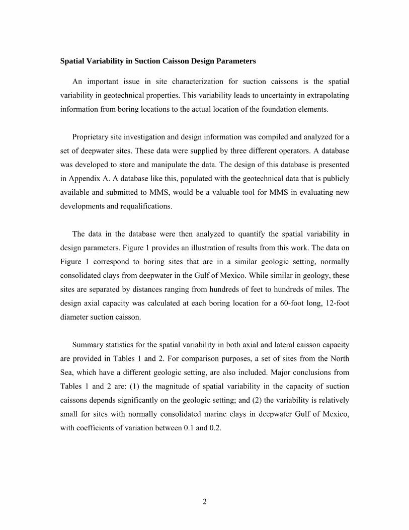
The data in the database were then analyzed to quantify the spatial variability in

design parameters. Figure 1 provides an illustration of results from this work. The data on

Figure 1 correspond to boring sites that are in a similar geologic setting, normally

consolidated clays from deepwater in the Gulf of Mexico. While similar in geology, these

sites are separated by distances ranging from hundreds of feet to hundreds of miles. The

design axial capacity was calculated at each boring location for a 60-foot long, 12-foot

diameter suction caisson.

Summary statistics for the spatial variability in both axial and lateral caisson capacity

are provided in Tables 1 and 2. For comparison purposes, a set of sites from the North

Sea, which have a different geologic setting, are also included. Major conclusions from

Tables 1 and 2 are: (1) the magnitude of spatial variability in the capacity of suction

caissons depends significantly on the geologic setting; and (2) the variability is relatively

small for sites with normally consolidated marine clays in deepwater Gulf of Mexico,

with coefficients of variation between 0.1 and 0.2.

2

Axial Suction Caisson CapacitiesLength = 60 ft, Diam. = 12 ft

0

200

400

600

800

1000

1200

1400

GO

M S

ite 1

GO

M S

ite 2

GO

M S

ite 3

GO

M S

ite 4

GO

M S

ite 5

GO

M S

ite 6

GO

M S

ite 7

GO

M S

ite 8

GO

M S

ite 9

Weight and Skin FrictionReverse End Bearing

Cap

acity

(kip

s)

Figure 1. Example of spatial variability in suction caisson capacity across Gulf of

Mexico deepwater boring sites.

Table 1. Summary statistics for spatial variability in total axial uplift capacity.

Length = 60 ft, Diameter = 12 ft

Sample Mean (kips)Sample Standard Deviation (kips) c. o. v.

GoM Sites 1076 100 0.09 North Sea Sites 1852 637 0.34 All Sites 1464 596 0.41




3

Table 2. Statistics relating to maximum lateral capacity. Length = 60 ft, Diameter = 12 ft






In order to better understand the spatial variability in suction caisson capacity, a

detailed simulation analysis was conducted (Gilbert and Murff 2001). For comparison

purposes, a typical driven steel pipe pile was also included in the analysis since this is the

conventional offshore foundation type for shallow water structures (Fig. 2). A generic

soil profile for a normally consolidated clay with an undrained shear strength increasing

at 10 psf/ft was used to simulate the variability in soil profiles that might exist across a

field (Fig. 3). A model presented in Smith and Gilbert (2001), which was calibrated with

data from one offshore field, was used to simulate this variability. Twenty-five soil

profiles were simulated; an example profile is shown on Fig. 4. The capacities for the

generic foundations were then calculated for each simulated profile using conventional

design practice (e.g., API 1993).

The results from this analysis are presented in Tables 3, 4 and 5. For axial side shear

(Table 3), the effect of variability in shear strength along the length of the pile is more

significant for a suction caisson than for a driven pile due to the effect of averaging.

Variations in strength tend to average along the length of the pile; intervals with lower

than average strength tend to be compensated by intervals with higher than average

strength. The longer the pile, the greater the effect of this averaging and the less

variability there is in the total skin friction. For axial end bearing, there is significantly

greater variability in end bearing than skin friction for both suction caissons and driven

piles (Table 4). The variability is greater for end bearing than skin friction because the

4

vertical extent of soil involved in the failure mechanism is smaller and there is less

averaging. Since end bearing contributes more to the total axial capacity for a suction

caisson than for a driven pile, variations in soil properties will have a greater effect on the

estimated end bearing for a suction caisson than for a driven pile. The total added effects

of side shear and end bearing are presented in Table 5. Note that there is substantially

more variability for a suction caisson that is loaded to failure in a pure lateral versus a

pure axial mode. This result occurs because a smaller region of shear effectively

contributes to the lateral capacity and there is less averaging than for the axial capacity.

In summary, uncertainties in soil properties will have a relatively greater effect on the

estimated axial capacity for a suction caisson compared to a driven pile, and they will

have a relatively greater effect on the lateral capacity than on the estimated axial capacity

for a suction caisson.

Fixed Jacket

Suction Caisson: Diameter = 12 feet Wall Thickness = 1.5 inches Length = 60 feet Pad Eye Location = 40 feet below Mudline

Floating Production

System

Driven Pile: Diameter = 42 inches Wall Thickness = 1.0 inches Length = 280 feet

Mudline

Figure 2. Schematic of generic suction caisson and driven pile.

5

Average Undrained Shear Strength: Intercept = 80 psf Slope = 10 psf/ft

Normally Consolidated Clay: PL = 25 LL = 70

Mudline

Figure 3. Generic soil profile.

0

50

100

150

200

250

300

0 1000 2000 3000 4000Design Strength (psf)

Dep

th (f

t)

Average Profile

Figure 4. Example of simulated strength profile.

6

Table 3. Comparison of total side friction for 25 simulated soil profiles.

Suction Caisson Driven Pile Average Total Side Friction (kips) 650 3,000 Standard Deviation in Total Side Friction (kips)

88 250

Coefficient of Variation in Total Side Friction 14 % 8 %

Table 4. Comparison of net end bearing for 25 simulated soil profile.s Suction Caisson Driven Pile Average Net End Bearing (kips) 580 250 Standard Deviation in Net End Bearing (kips) 230 58 Coefficient of Variation in Net End Bearing 39 % 23 % Average Contribution to Total Capacity 42 % 7 %

Table 5. Variability in total capacity for 25 simulated soil profiles. Suction Caisson Driven Pile Coefficient of Variation in Axial Capacity 21 % 8 % Coefficient of Variation in Lateral Capacity 33 % Not Relevant

7

Calibration of Suction Caisson Design Method

In order to understand the effect of uncertainty from site characterization programs on

design, the first step is to assess the magnitude of uncertainty in the design method itself

(i.e., even if a soil boring exists at the location of a suction caisson, the actual capacity is

still uncertain due to uncertainty in the design method). In this way, the relative

contribution of uncertainty that can be controlled through site characterization is

considered in the proper perspective of the overall uncertainty in the design capacity.

Design methods and criteria for the capacity of suction caissons have generally been

adapted from those for driven pipe piles (Andersen et al. 1999). However, the accuracy of

these design methods has never been thoroughly tested due to the lack of published

databases of pullout tests on suction caissons. A database that is comprised of published

laboratory model tests, centrifuge tests, and full scale field tests conducted on suction

caissons in normally consolidated clays was assembled and used to evaluate biases and

uncertainties that are inherent in available models for predicting the uplift capacity of

suction caissons in normally consolidated clays.

Capacity for Axial (Uplift) Loading

The axial capacity of a suction caisson, which generally governs design in practical

applications even for inclined loading conditions, is comprised of side shear and reverse

end bearing. Under rapid uplift loading, the side resistance is typically calculated using a

variation of the alpha method as a function of the undrained shearing strength of the soil.

For normally consolidated clays, an alpha value of near 1.0 is typically used in the design

of offshore piles. For suction caissons, concerns about the effect of suction installation,

soil setup, and the presence of the padeye have led to a tendency for designers to reduce

alpha to values that are less than 1.0 (α = 0.6 to 0.8). Randolph and House (2002) indicate

that after installation, the external side resistance is expected to increase from the soil’s

remolded strength to a fully equalized strength that corresponds to alpha values of about

0.5 to 0.7. The fact that alpha does not reach a value of 1.0 is attributed by the authors to

8

the high ratio of diameter to wall thickness of suction caissons. Andersen and Jostad

(1999) and Clukey (2001) state that an expected reduction in the external skin friction for

the full set-up condition can be attributed to a reduction in soil stresses on the portion of

the caisson that is installed with suction. The rationale behind such a concern is the

observation that the soil typically moves into the caisson (rather than outside the caisson)

as a result of installation by suction.

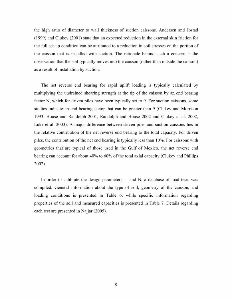
The net reverse end bearing for rapid uplift loading is typically calculated by

multiplying the undrained shearing strength at the tip of the caisson by an end bearing

factor N, which for driven piles have been typically set to 9. For suction caissons, some

studies indicate an end bearing factor that can be greater than 9 (Clukey and Morrison

1993, House and Randolph 2001, Randolph and House 2002 and Clukey et al. 2002,

Luke et al. 2003). A major difference between driven piles and suction caissons lies in

the relative contribution of the net reverse end bearing to the total capacity. For driven

piles, the contribution of the net end bearing is typically less than 10%. For caissons with

geometries that are typical of those used in the Gulf of Mexico, the net reverse end

bearing can account for about 40% to 60% of the total axial capacity (Clukey and Phillips

2002).

In order to calibrate the design parameters � and N, a database of load tests was

compiled. General information about the type of soil, geometry of the caisson, and

loading conditions is presented in Table 6, while specific information regarding

properties of the soil and measured capacities is presented in Table 7. Details regarding

each test are presented in Najjar (2005).

9

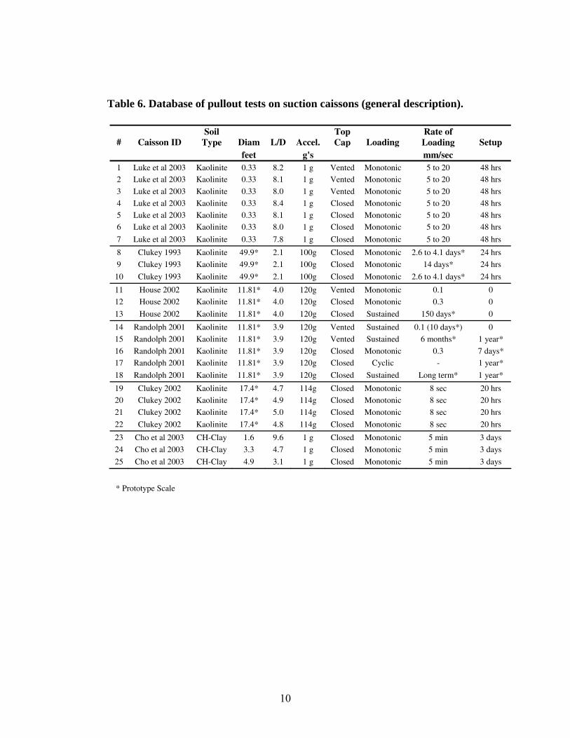
Table 6. Database of pullout tests on suction caissons (general description).

# Caisson ID Soil

Type Diam L/D Accel. Top Cap Loading

Rate of Loading Setup

feet g's mm/sec 1 Luke et al 2003 Kaolinite 0.33 8.2 1 g Vented Monotonic 5 to 20 48 hrs

2 Luke et al 2003 Kaolinite 0.33 8.1 1 g Vented Monotonic 5 to 20 48 hrs

3 Luke et al 2003 Kaolinite 0.33 8.0 1 g Vented Monotonic 5 to 20 48 hrs

4 Luke et al 2003 Kaolinite 0.33 8.4 1 g Closed Monotonic 5 to 20 48 hrs




8 Clukey 1993 Kaolinite 49.9* 2.1 100g Closed Monotonic 2.6 to 4.1 days* 24 hrs

9 Clukey 1993 Kaolinite 49.9* 2.1 100g Closed Monotonic 14 days* 24 hrs

10 Clukey 1993 Kaolinite 49.9* 2.1 100g Closed Monotonic 2.6 to 4.1 days* 24 hrs

11 House 2002 Kaolinite 11.81* 4.0 120g Vented Monotonic 0.1 0

12 House 2002 Kaolinite 11.81* 4.0 120g Closed Monotonic 0.3 0

13 House 2002 Kaolinite 11.81* 4.0 120g Closed Sustained 150 days* 0

14 Randolph 2001 Kaolinite 11.81* 3.9 120g Vented Sustained 0.1 (10 days*) 0

15 Randolph 2001 Kaolinite 11.81* 3.9 120g Vented Sustained 6 months* 1 year*

16 Randolph 2001 Kaolinite 11.81* 3.9 120g Closed Monotonic 0.3 7 days*

17 Randolph 2001 Kaolinite 11.81* 3.9 120g Closed Cyclic - 1 year*

18 Randolph 2001 Kaolinite 11.81* 3.9 120g Closed Sustained Long term* 1 year*

19 Clukey 2002 Kaolinite 17.4* 4.7 114g Closed Monotonic 8 sec 20 hrs




23 Cho et al 2003 CH-Clay 1.6 9.6 1 g Closed Monotonic 5 min 3 days



* Prototype Scale

10

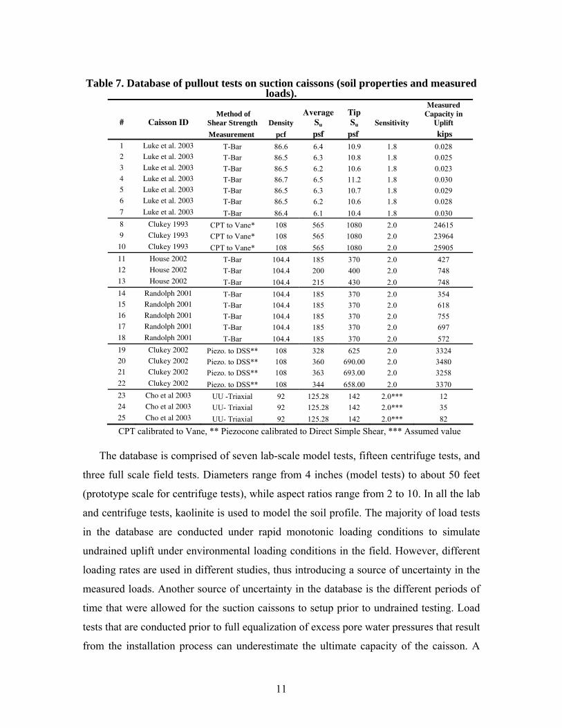
Table 7. Database of pullout tests on suction caissons (soil properties and measured

loads).

# Caisson ID Method of

Shear Strength Density Average

Su Tip Su Sensitivity

Measured Capacity in

Uplift Measurement pcf psf psf kips 1 Luke et al. 2003 T-Bar 86.6 6.4 10.9 1.8 0.028 2 Luke et al. 2003 T-Bar 86.5 6.3 10.8 1.8 0.025 3 Luke et al. 2003 T-Bar 86.5 6.2 10.6 1.8 0.023 4 Luke et al. 2003 T-Bar 86.7 6.5 11.2 1.8 0.030 5 Luke et al. 2003 T-Bar 86.5 6.3 10.7 1.8 0.029 6 Luke et al. 2003 T-Bar 86.5 6.2 10.6 1.8 0.028 7 Luke et al. 2003 T-Bar 86.4 6.1 10.4 1.8 0.030 8 Clukey 1993 CPT to Vane* 108 565 1080 2.0 24615 9 Clukey 1993 CPT to Vane* 108 565 1080 2.0 23964 10 Clukey 1993 CPT to Vane* 108 565 1080 2.0 25905 11 House 2002 T-Bar 104.4 185 370 2.0 427 12 House 2002 T-Bar 104.4 200 400 2.0 748 13 House 2002 T-Bar 104.4 215 430 2.0 748 14 Randolph 2001 T-Bar 104.4 185 370 2.0 354 15 Randolph 2001 T-Bar 104.4 185 370 2.0 618 16 Randolph 2001 T-Bar 104.4 185 370 2.0 755 17 Randolph 2001 T-Bar 104.4 185 370 2.0 697 18 Randolph 2001 T-Bar 104.4 185 370 2.0 572 19 Clukey 2002 Piezo. to DSS** 108 328 625 2.0 3324 20 Clukey 2002 Piezo. to DSS** 108 360 690.00 2.0 3480 21 Clukey 2002 Piezo. to DSS** 108 363 693.00 2.0 3258 22 Clukey 2002 Piezo. to DSS** 108 344 658.00 2.0 3370 23 Cho et al 2003 UU -Triaxial 92 125.28 142 2.0*** 12 24 Cho et al 2003 UU- Triaxial 92 125.28 142 2.0*** 35 25 Cho et al 2003 UU- Triaxial 92 125.28 142 2.0*** 82 CPT calibrated to Vane, ** Piezocone calibrated to Direct Simple Shear, *** Assumed value

The database is comprised of seven lab-scale model tests, fifteen centrifuge tests, and

three full scale field tests. Diameters range from 4 inches (model tests) to about 50 feet

(prototype scale for centrifuge tests), while aspect ratios range from 2 to 10. In all the lab

and centrifuge tests, kaolinite is used to model the soil profile. The majority of load tests

in the database are conducted under rapid monotonic loading conditions to simulate

undrained uplift under environmental loading conditions in the field. However, different

loading rates are used in different studies, thus introducing a source of uncertainty in the

measured loads. Another source of uncertainty in the database is the different periods of

time that were allowed for the suction caissons to setup prior to undrained testing. Load

tests that are conducted prior to full equalization of excess pore water pressures that result

from the installation process can underestimate the ultimate capacity of the caisson. A

11

last major source of uncertainty in the database lies in the use of different methods to

measure the undrained shearing strength of the soil. A variety of direct simple shear,

unconsolidated-undrained triaxial, cone penetration, vane shear, and T-bar tests are used

to measure the undrained shearing strength in the different case studies analyzed.

In an initial analysis of the database, predicted capacities for the 25 tests were

calculated using � = 1 and N = 9. Values of undrained strength that were reported in the

original references were used in this initial analysis with no attempts to correct for the

method of shear strength measurement. For pullout tests that were conducted

immediately after installation (Tests 11 to 14), the undrained shearing strength of the

remolded clay was used in calculating the predicted side shear capacity. Ratios of

measured to predicted capacities for the 25 tests in the database are plotted on Figure 1.

Results on Figure 5 indicate an average ratio of measured to predicted capacity of 0.99

(unbiased model) and a coefficient of variation in the ratio of measured to predicted

capacity of 0.28.

0.0

0.5

1.0

1.5

2.0

0.0 0.1 1.0 10.0 100.0 1000.0 10000.0 100000.0

Measured Capacity (kips)

Mea

sure

d C

apac

ity /

Pred

icte

d C

apac

ity

Luke et al 2003Clukey and Morrison 1993Clukey et al 2003Randolph and House 2002Cho et al 2003House and Randolph 2001

Figure 5. Comparison between measured and predicted capacities for 25 suction caissons (uncorrected shear strength, α = 1, N = 9).

12

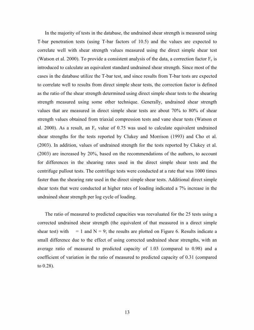
In the majority of tests in the database, the undrained shear strength is measured using

T-bar penetration tests (using T-bar factors of 10.5) and the values are expected to

correlate well with shear strength values measured using the direct simple shear test

(Watson et al. 2000). To provide a consistent analysis of the data, a correction factor Fc is

introduced to calculate an equivalent standard undrained shear strength. Since most of the

cases in the database utilize the T-bar test, and since results from T-bar tests are expected

to correlate well to results from direct simple shear tests, the correction factor is defined

as the ratio of the shear strength determined using direct simple shear tests to the shearing

strength measured using some other technique. Generally, undrained shear strength

values that are measured in direct simple shear tests are about 70% to 80% of shear

strength values obtained from triaxial compression tests and vane shear tests (Watson et

al. 2000). As a result, an Fc value of 0.75 was used to calculate equivalent undrained

shear strengths for the tests reported by Clukey and Morrison (1993) and Cho et al.

(2003). In addition, values of undrained strength for the tests reported by Clukey et al.

(2003) are increased by 20%, based on the recommendations of the authors, to account

for differences in the shearing rates used in the direct simple shear tests and the

centrifuge pullout tests. The centrifuge tests were conducted at a rate that was 1000 times

faster than the shearing rate used in the direct simple shear tests. Additional direct simple

shear tests that were conducted at higher rates of loading indicated a 7% increase in the

undrained shear strength per log cycle of loading.

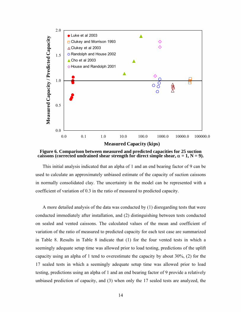
The ratio of measured to predicted capacities was reevaluated for the 25 tests using a

corrected undrained shear strength (the equivalent of that measured in a direct simple

shear test) with � = 1 and N = 9; the results are plotted on Figure 6. Results indicate a

small difference due to the effect of using corrected undrained shear strengths, with an

average ratio of measured to predicted capacity of 1.03 (compared to 0.98) and a

coefficient of variation in the ratio of measured to predicted capacity of 0.31 (compared

to 0.28).

13

0.0

0.5

1.0

1.5

2.0

0.0 0.1 1.0 10.0 100.0 1000.0 10000.0 100000.0

Measured Capacity (kips)

Mea

sure

d C

apac

ity /

Pred

icte

d C

apac

ity

Luke et al 2003Clukey and Morrison 1993Clukey et al 2003Randolph and House 2002Cho et al 2003House and Randolph 2001

Figure 6. Comparison between measured and predicted capacities for 25 suction

caissons (corrected undrained shear strength for direct simple shear, α = 1, N = 9). This initial analysis indicated that an alpha of 1 and an end bearing factor of 9 can be

used to calculate an approximately unbiased estimate of the capacity of suction caissons

in normally consolidated clay. The uncertainty in the model can be represented with a

coefficient of variation of 0.3 in the ratio of measured to predicted capacity.

A more detailed analysis of the data was conducted by (1) disregarding tests that were

conducted immediately after installation, and (2) distinguishing between tests conducted

on sealed and vented caissons. The calculated values of the mean and coefficient of

variation of the ratio of measured to predicted capacity for each test case are summarized

in Table 8. Results in Table 8 indicate that (1) for the four vented tests in which a

seemingly adequate setup time was allowed prior to load testing, predictions of the uplift

capacity using an alpha of 1 tend to overestimate the capacity by about 30%, (2) for the

17 sealed tests in which a seemingly adequate setup time was allowed prior to load

testing, predictions using an alpha of 1 and an end bearing factor of 9 provide a relatively

unbiased prediction of capacity, and (3) when only the 17 sealed tests are analyzed, the

14

uncertainty in the prediction model decreases noticeably; the coefficient of variation in

the ratio of the measured to predicted capacity decreases to 0.17 or 0.25, depending on

whether the uncorrected or corrected undrained shear strength values are used in

predicting capacity.

Table 8. Biases and uncertainties in model for suction caissons (α=1, N=9).

Number of Tests

Average for Ratio of

Measured to Predicted

Coefficient of Variation for Ratio of

Measured to Predicted

All Tests 25 0.99 0.28

All Tests with Setup 21 0.92 0.20

Sealed Tests with Setup 17 0.97 0.17

Unc

orre

cted

Und

rain

ed

Shea

r Stre

ngth

Vented Tests with Setup 4 0.71 0.16

All Tests 25 1.03 0.31

All Tests with Setup 21 0.97 0.28

Sealed Tests with Setup 17 1.03 0.25

Cor

rect

ed D

irect

Sim

ple

Shea

r Stre

ngth

Vented Tests with Setup 4 0.71 0.16

While values of α = 1 and N = 9 provide reasonably unbiased results, there is actually

a range of combinations of α = 1 and N = 9 that can produce unbiased results since a

single value, the total axial capacity, is measured in the load tests. Combinations of α and

N that resulted in an unbiased model were calculated and presented in Table 9.

Coefficients of variation in the ratio of measured to predicted capacity corresponding to

these combinations of α and N were also calculated (Table 9). Tests where the caissons

were pulled out immediately after installation (no set up) were excluded from the

analysis. Results indicate that different combinations of α and N can be used to predict

15

the measured capacities in an unbiased manner. For values of α ranging from 0.7 to 1, the

corresponding N factors range from 13 to 8.5, respectively, while corresponding c.o.v’s

range from 0.26 to 0.28. It should be noted that the combination of α = 0.7 and N = 13

provides an unbiased estimate for both the vented tests and the sealed tests even when

analyzed separately.

Table 9. Calibration of α and N (corrected undrained shear strength and excluding

tests with setup = 0).

Measured Capacity / Predicted Capacity α N Average Coefficient of Variation

1.0 8.5 1.0 0.28 0.9 9.7 1.0 0.27 0.8 11.2 1.0 0.26 0.7 13 1.0 0.26

As a final piece of information on the calibrated design method, El-Sherbiny (2005)

conducted 1-g model tests with a double-walled caisson where the contribution of side

shear and end bearing could be separated. El-Sherbiny found from four tests that an

average alpha of 0.78 and an average N of 15 were mobilized at the failure load.

Conversely, Jeanjean et al. (2006) conducted centrifuge model tests with a double-walled

caisson and measured an alpha of 0.85 and N of 9. Jeanjean et al. (2006) actually

measured a value greater than 12 for N at a displacement of about 10% of the caisson

diameter; however, the maximum side shear was mobilized at about one-tenth of that

displacement. Chen and Randolph (2005) reported an alpha factor of 0.76 and an N value

of 12 to match their test results.

Therefore, the appropriate combination of alpha and N is on the order of � = 0.8 and

N = 12 based on all of the available information. This combination will produce a

reasonably unbiased estimate of the uplift capacity for a suction caisson, with a

coefficient of variation of about 0.3 between the actual and estimated capacity. For

comparison purposes, similar analyses for driven piles produce a coefficient of variation

for the design method that is between 0.2 and 0.3 (Najjar 2005).

16

Capacity for Lateral and Inclined Loading

The capacity for suction caissons on lateral and inclined loading is calculated using a

combination of the method described and calibrated above for axial capacity and a

method developed by Aubeny and Murff on an OTRC project at TAMU (referred to here

s the SAIL method). In order to provide information for calibrating the SAIL method, El-

Sherbiny (2005) ran a series of seven 1-g model tests with undrained loading and a loa

attachment at the lower third point of the caisson (typical for practice). The tests covered

the entire range of angles from horizontal to vertical, which provides a complete set of

data for verification of the design method. The experimental results, shown on Fig. 7,

compare very well with analyses performed using the SAIL method with � = 0.78 and N

= 15.

0

10

20

30

40

50

60

0 20 40 60 80Horizontal component of capacity (lb)

Vert

ical

com

pone

nt o

f cap

acity

(lb)

100

Measured ValuesSAIL: α=0.78, Nc=15

30o

10o

20o

45o

Figure 7. Comparison between measured and predicted components of suction

caisson capacity under inclined loading (El-Sherbiny 2005).

Lower-Bound Capacity

One general concern arising from the work on spatial variability and model

calibration is the magnitude of uncertainty for suction caisson design is generally larger

than that for driven piles in normally consolidated clays. One possible mitigating factor is

the effect of a lower-bound capacity in limiting the uncertainty (e.g., Gilbert 2003, Najjar

2005 and Gilbert et al. 2005).

17

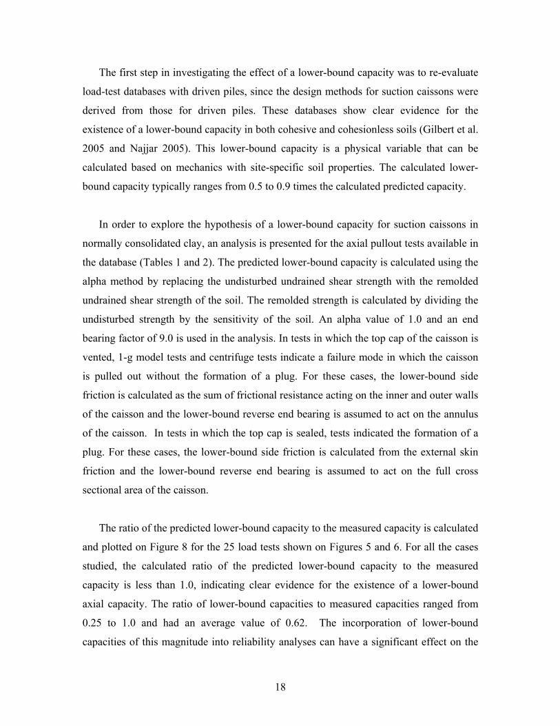
The first step in investigating the effect of a lower-bound capacity was to re-evaluate

load-test databases with driven piles, since the design methods for suction caissons were

derived from those for driven piles. These databases show clear evidence for the

existence of a lower-bound capacity in both cohesive and cohesionless soils (Gilbert et al.

2005 and Najjar 2005). This lower-bound capacity is a physical variable that can be

calculated based on mechanics with site-specific soil properties. The calculated lower-

bound capacity typically ranges from 0.5 to 0.9 times the calculated predicted capacity.

In order to explore the hypothesis of a lower-bound capacity for suction caissons in

normally consolidated clay, an analysis is presented for the axial pullout tests available in

the database (Tables 1 and 2). The predicted lower-bound capacity is calculated using the

alpha method by replacing the undisturbed undrained shear strength with the remolded

undrained shear strength of the soil. The remolded strength is calculated by dividing the

undisturbed strength by the sensitivity of the soil. An alpha value of 1.0 and an end

bearing factor of 9.0 is used in the analysis. In tests in which the top cap of the caisson is

vented, 1-g model tests and centrifuge tests indicate a failure mode in which the caisson

is pulled out without the formation of a plug. For these cases, the lower-bound side

friction is calculated as the sum of frictional resistance acting on the inner and outer walls

of the caisson and the lower-bound reverse end bearing is assumed to act on the annulus

of the caisson. In tests in which the top cap is sealed, tests indicated the formation of a

plug. For these cases, the lower-bound side friction is calculated from the external skin

friction and the lower-bound reverse end bearing is assumed to act on the full cross

sectional area of the caisson.

The ratio of the predicted lower-bound capacity to the measured capacity is calculated

and plotted on Figure 8 for the 25 load tests shown on Figures 5 and 6. For all the cases

studied, the calculated ratio of the predicted lower-bound capacity to the measured

capacity is less than 1.0, indicating clear evidence for the existence of a lower-bound

axial capacity. The ratio of lower-bound capacities to measured capacities ranged from

0.25 to 1.0 and had an average value of 0.62. The incorporation of lower-bound

capacities of this magnitude into reliability analyses can have a significant effect on the

18

calculated reliability of suction caissons in normally consolidated clays. This effect is

considered in the next section of this report.

0.0

0.5

1.0

1.5

2.0

0.0 0.1 1.0 10.0 100.0 1000.0 10000.0 100000.0Measured Capacity (kips)

Low

er B

ound

/ M

easu

red

Cap

acity

Luke et al 2003Clukey and Morrison 1993

Clukey et al 2002

Randolph and House 2002

Cho et al 2003

House and Randolph 2001

Figure 8. Evidence of Lower-Bound Capacity for 25 Suction Caissons

19

Reliability-Based Design of Suction Caissons A conventional reliability analysis for an offshore foundation provides a useful

framework as a starting point to consider the reliability of the suction caissons for the

study spar. A conventional reliability analysis can be generalized in a convenient

mathematical form as follows:

( ) ( )median2 2load capacity

ln FSLoad CapacityP

⎛ ⎞⎜> −⎜⎜ ⎟δ +δ⎝ ⎠

≅ Φ ⎟⎟ (1)

where P(Load > Capacity) is the probability that the load exceeds the capacity in the

design life, which is also referred to as the lifetime probability of failure; FSmedian is the

median factor of safety, which is defined as the ratio of the median capacity to the

median load; and � is the coefficient of variation (c.o.v.), which is defined as the

standard deviation divided by the mean value for that variable. Equation 1 assumes that

the load and capacity each follow lognormal distributions, a common assumption in

typical reliability analyses for offshore foundations (e.g., Tang and Gilbert 1993).

The median factor of safety in Equation 1 can be related to the factor of safety used in

design:

median

designmedian design

median

design

capacitycapacity

FS FSloadload

⎛ ⎞⎜ ⎟⎜ ⎟⎝= ×⎛ ⎞⎜ ⎟⎜ ⎟⎝ ⎠

⎠ (2)

where the subscript “design” indicates the value used to design the foundation. The ratios

of the median to design values represent biases between the median or most likely value

in the design life and the value that is used in the design check with the factor of safety.

For context, the median factor of safety is between three and five for a pile in a typical

jacket platform.

The coefficients of variation in Equation 1 represent uncertainty in the load and the

capacity. For an offshore foundation, the uncertainty in the load is generally due to

variations in the occurrence and strength of hurricanes at the platform site over the design

20

life. The uncertainty in the capacity is due primarily to variations between the actual

capacity in a storm load compared to the capacity predicted using the design method. The

denominator in Equation 1 is referred to as the total coefficient of variation:

2 2total load capacity=δ δ + δ (3)

As an example, typical c.o.v. values for a jacket platform range from 0.3 to 0.5 for the

load, 0.3 to 0.5 for the capacity, and 0.5 to 0.7 for the total.

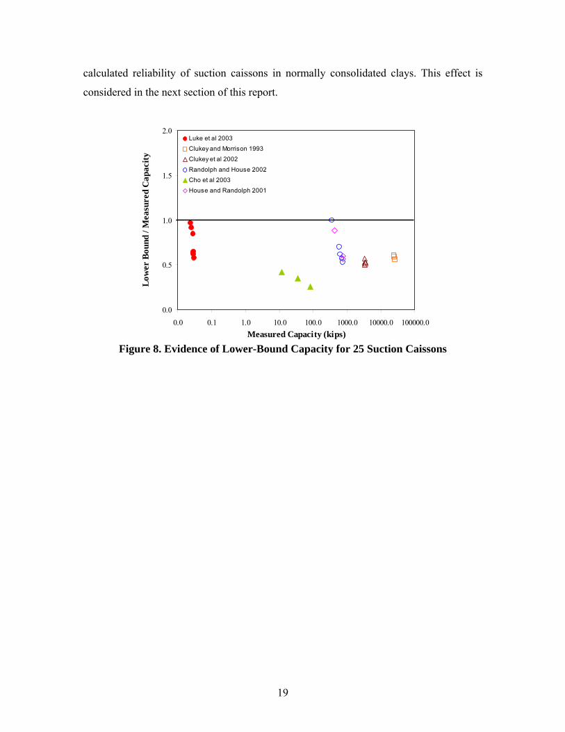
The relationship between the probability of failure and the median factor of safety

and the total c.o.v. is shown on Figure 9. An increase in the median factor of safety and a

decrease in the total c.o.v. both reduce the probability of failure. For context, the lifetime

failure probabilities for a pile in a typical jacket foundation range from 0.005 to 0.05 (Fig.

9). Note that the event of foundation failure, i.e. axial overload of a single pile in the

foundation, does not necessarily lead to collapse of a jacket. Failure probabilities for the

foundation system are ten to 100 times smaller than those for a single pile (Tang and

Gilbert 1993).

0.00001

0.0001

0.001

0.01

0.1

11 2 3 4 5 6 7 8 9 10

FSmedian

Pro

babi

lity

of F

ound

atio

n Fa

ilure

in L

ifetim

e

Total c.o.v. = 0.7

0.60.5

Typical for

Jackets

0.40.3

Figure 9. Results from a conventional reliability analysis on a pile in a typical jacket

platform.

21

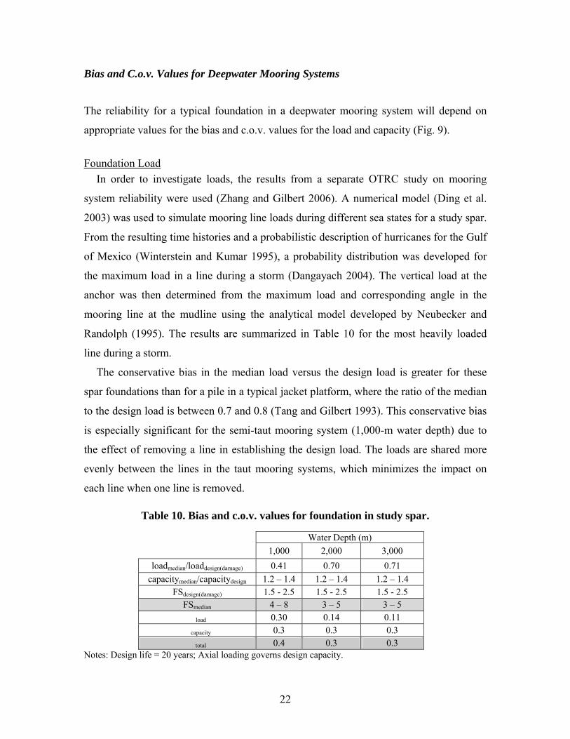
Bias and C.o.v. Values for Deepwater Mooring Systems

The reliability for a typical foundation in a deepwater mooring system will depend on

appropriate values for the bias and c.o.v. values for the load and capacity (Fig. 9).

Foundation Load In order to investigate loads, the results from a separate OTRC study on mooring

system reliability were used (Zhang and Gilbert 2006). A numerical model (Ding et al.

2003) was used to simulate mooring line loads during different sea states for a study spar.

From the resulting time histories and a probabilistic description of hurricanes for the Gulf

of Mexico (Winterstein and Kumar 1995), a probability distribution was developed for

the maximum load in a line during a storm (Dangayach 2004). The vertical load at the

anchor was then determined from the maximum load and corresponding angle in the

mooring line at the mudline using the analytical model developed by Neubecker and

Randolph (1995). The results are summarized in Table 10 for the most heavily loaded

line during a storm.

The conservative bias in the median load versus the design load is greater for these

spar foundations than for a pile in a typical jacket platform, where the ratio of the median

to the design load is between 0.7 and 0.8 (Tang and Gilbert 1993). This conservative bias

is especially significant for the semi-taut mooring system (1,000-m water depth) due to

the effect of removing a line in establishing the design load. The loads are shared more

evenly between the lines in the taut mooring systems, which minimizes the impact on

each line when one line is removed.

Table 10. Bias and c.o.v. values for foundation in study spar.

Water Depth (m) 1,000 2,000 3,000

loadmedian/loaddesign(damage) 0.41 0.70 0.71 capacitymedian/capacitydesign 1.2 – 1.4 1.2 – 1.4 1.2 – 1.4

FSdesign(damage) 1.5 - 2.5 1.5 - 2.5 1.5 - 2.5 FSmedian 4 – 8 3 – 5 3 – 5

�load 0.30 0.14 0.11 �capacity 0.3 0.3 0.3

�total 0.4 0.3 0.3 Notes: Design life = 20 years; Axial loading governs design capacity.

22

Also, the coefficients of variation in the spar foundation load are smaller than for a

pile in a typical jacket platform, where the c.o.v. values are generally between 0.3 and 0.5

(Tang and Gilbert 1993). There are several reasons for smaller uncertainty in the

foundation loads on the spar. First, the line loads are less sensitive to wave height for a

spar mooring system in deep water compared to a fixed jacket in shallow water (e.g.,

Banon and Harding 1989). Therefore, variations in the sea states over the design life are

less significant for the spar mooring system. Second, the mooring system is simpler to

model than a jacket, meaning that there is less uncertainty in the loads predicted by the

model. Finally, the spar line loads are dominated by pre-tension versus environmental

loads; variations in the load due to variations in the sea states therefore have a smaller

effect on the total line load. This effect of pre-tension is particularly significant for the

taut mooring systems (2,000-m and 3,000-m water depths), which consequently have the

smallest c.o.v. values (Table 1).

Foundation Capacity The work described above on spatial variability and calibrating the design method

provide a basis for establishing the coefficient of variation in the capacity. For c.o.v.

values of 0.25 to 0.3 in the design method and 0.1 to 0.2 for spatial variability due to soil

borings not located at each foundation site, the total c.o.v. in capacity is 0.3 to 0.35. This

value is very similar to the value of 0.3 that is typically used for pile foundations on

jacket platforms (Tang and Gilbert 1993).

Median Factor of Safety, Total c.o.v. and Reliability The biases in the load and the capacity are combined together with the design factor

of safety through Equation 2 to determine the median factor of safety, and the results are

summarized in Table 10. Typical factors of safety being used in practice for the damage

case, which governs design for the study spar, range between 1.5 and 2.5. In addition, the

total c.o.v. values are obtained from Equation 3 (Table 10).

The relationship between the reliability and FSmedian and �total is re-plotted on Figure

10. For the spar foundation, the probability that the axial load will exceed the capacity of

the suction caisson during a 20-year design life is on the order of 0.0001 or smaller. For

23

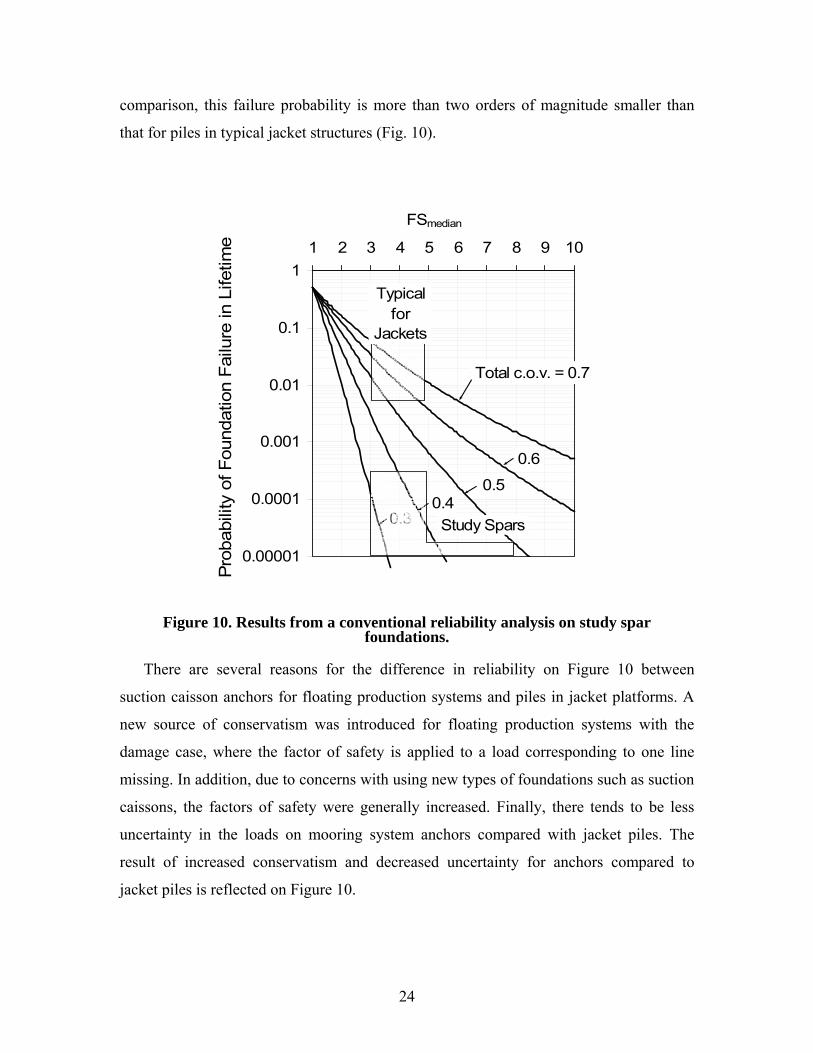
comparison, this failure probability is more than two orders of magnitude smaller than

that for piles in typical jacket structures (Fig. 10).

0.00001

0.0001

0.001

0.01

0.1

11 2 3 4 5 6 7 8 9 10

FSmedianPr

obab

ility

of F

ound

atio

n Fa

ilure

in L

ifetim

e

Total c.o.v. = 0.7

0.6

0.5

Typical for

Jackets

0.40.3 Study Spars

Figure 10. Results from a conventional reliability analysis on study spar foundations.

There are several reasons for the difference in reliability on Figure 10 between

suction caisson anchors for floating production systems and piles in jacket platforms. A

new source of conservatism was introduced for floating production systems with the

damage case, where the factor of safety is applied to a load corresponding to one line

missing. In addition, due to concerns with using new types of foundations such as suction

caissons, the factors of safety were generally increased. Finally, there tends to be less

uncertainty in the loads on mooring system anchors compared with jacket piles. The

result of increased conservatism and decreased uncertainty for anchors compared to

jacket piles is reflected on Figure 10.

24

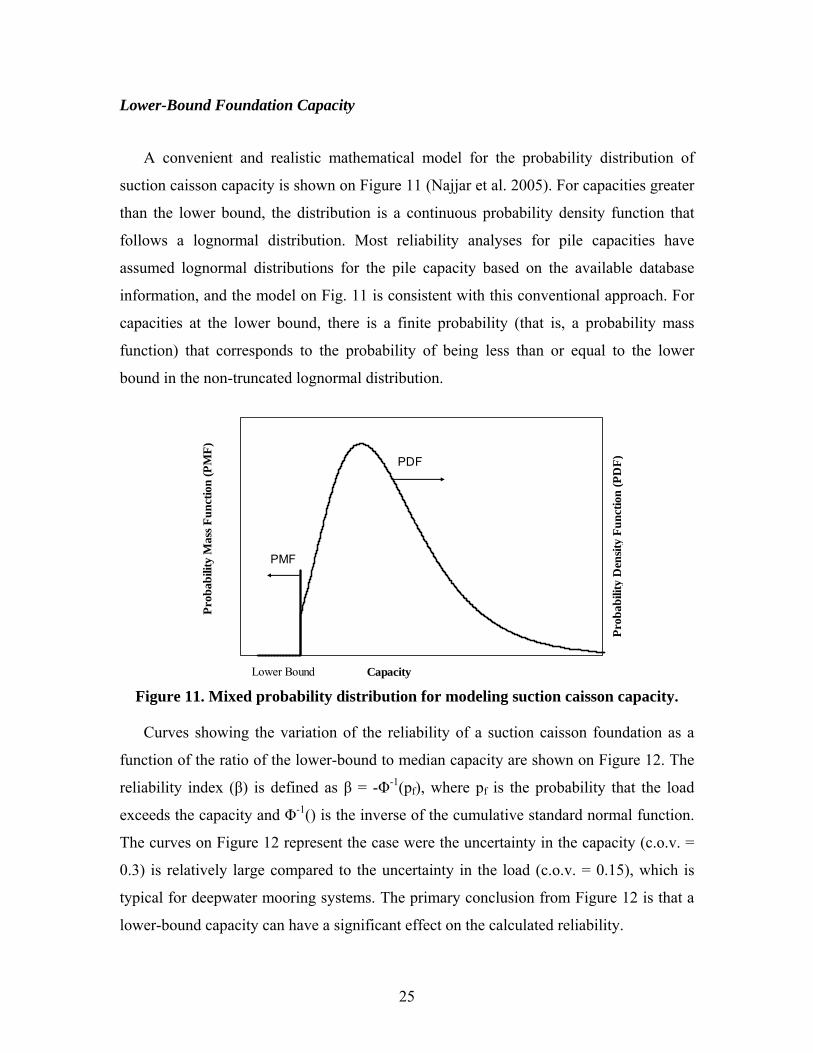
Lower-Bound Foundation Capacity

A convenient and realistic mathematical model for the probability distribution of

suction caisson capacity is shown on Figure 11 (Najjar et al. 2005). For capacities greater

than the lower bound, the distribution is a continuous probability density function that

follows a lognormal distribution. Most reliability analyses for pile capacities have

assumed lognormal distributions for the pile capacity based on the available database

information, and the model on Fig. 11 is consistent with this conventional approach. For

capacities at the lower bound, there is a finite probability (that is, a probability mass

function) that corresponds to the probability of being less than or equal to the lower

bound in the non-truncated lognormal distribution.

Prob

abili

ty D

ensit

y Fu

nctio

n (P

DF)

Prob

abili

ty M

ass F

unct

ion

(PM

F)

Lower Bound Capacity

PDF

PMF

Figure 11. Mixed probability distribution for modeling suction caisson capacity.

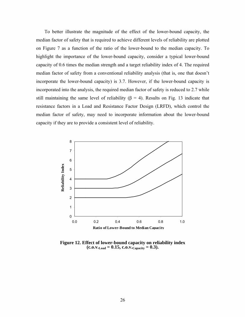
Curves showing the variation of the reliability of a suction caisson foundation as a

function of the ratio of the lower-bound to median capacity are shown on Figure 12. The

reliability index (β) is defined as β = -Φ-1(pf), where pf is the probability that the load

exceeds the capacity and Φ-1() is the inverse of the cumulative standard normal function.

The curves on Figure 12 represent the case were the uncertainty in the capacity (c.o.v. =

0.3) is relatively large compared to the uncertainty in the load (c.o.v. = 0.15), which is

typical for deepwater mooring systems. The primary conclusion from Figure 12 is that a

lower-bound capacity can have a significant effect on the calculated reliability.

25

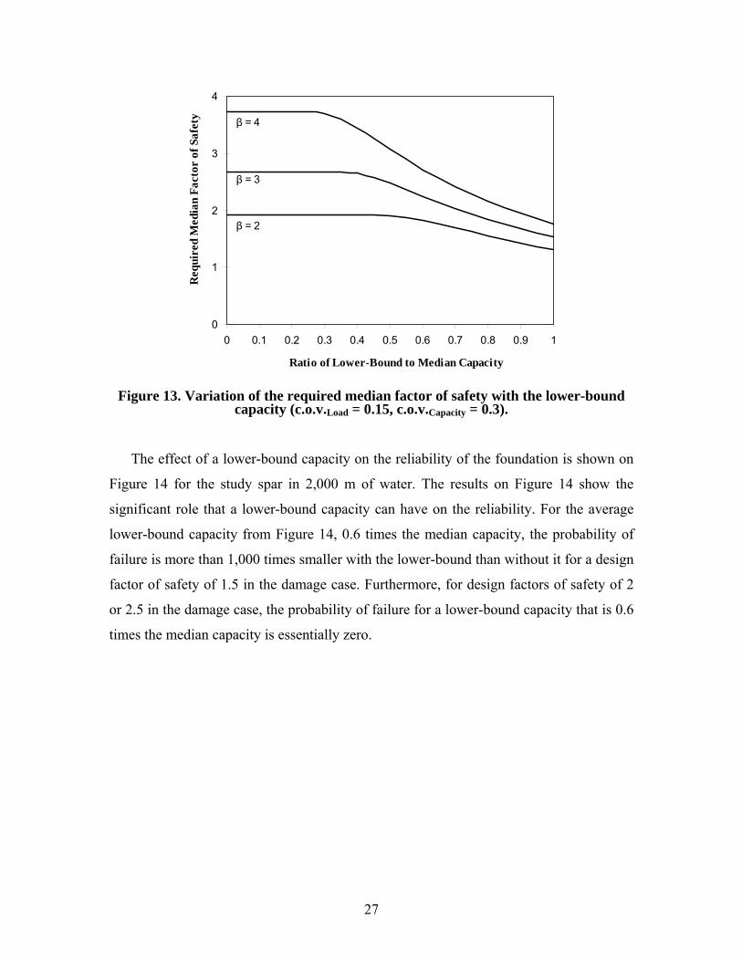
To better illustrate the magnitude of the effect of the lower-bound capacity, the

median factor of safety that is required to achieve different levels of reliability are plotted

on Figure 7 as a function of the ratio of the lower-bound to the median capacity. To

highlight the importance of the lower-bound capacity, consider a typical lower-bound

capacity of 0.6 times the median strength and a target reliability index of 4. The required

median factor of safety from a conventional reliability analysis (that is, one that doesn’t

incorporate the lower-bound capacity) is 3.7. However, if the lower-bound capacity is

incorporated into the analysis, the required median factor of safety is reduced to 2.7 while

still maintaining the same level of reliability (β = 4). Results on Fig. 13 indicate that

resistance factors in a Load and Resistance Factor Design (LRFD), which control the

median factor of safety, may need to incorporate information about the lower-bound

capacity if they are to provide a consistent level of reliability.

0

1

2

3

4

5

6

7

8

0.0 0.2 0.4 0.6 0.8 1.0

Ratio of Lower-Bound to Median Capacity

Rel

iabi

lity

Inde

x

Figure 12. Effect of lower-bound capacity on reliability index

(c.o.v.Load = 0.15, c.o.v.Capacity = 0.3).

26

0

1

2

3

4

0 0.1 0.2 0.3 0.4 0.5 0.6 0.7 0.8 0.9 1


Req

uire

d M

edia

n Fa

ctor

of S

afet

y β = 4

β = 2

β = 3

Figure 13. Variation of the required median factor of safety with the lower-bound capacity (c.o.v.Load = 0.15, c.o.v.Capacity = 0.3).

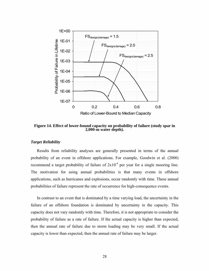
The effect of a lower-bound capacity on the reliability of the foundation is shown on

Figure 14 for the study spar in 2,000 m of water. The results on Figure 14 show the

significant role that a lower-bound capacity can have on the reliability. For the average

lower-bound capacity from Figure 14, 0.6 times the median capacity, the probability of

failure is more than 1,000 times smaller with the lower-bound than without it for a design

factor of safety of 1.5 in the damage case. Furthermore, for design factors of safety of 2

or 2.5 in the damage case, the probability of failure for a lower-bound capacity that is 0.6

times the median capacity is essentially zero.

27

1E-07

1E-06

1E-05

1E-04

1E-03

1E-02

1E-01

1E+00

0 0.2 0.4 0.6 0.8Ratio of Lower-Bound to Median Capacity

Pro

babi

lity

of F

ailu

re in

Life

time

FSdesign(damage) = 1.5



Figure 14. Effect of lower-bound capacity on probability of failure (study spar in 2,000-m water depth).

Target Reliability

Results from reliability analyses are generally presented in terms of the annual

probability of an event in offshore applications. For example, Goodwin et al. (2000)

recommend a target probability of failure of 2x10-4 per year for a single mooring line.

The motivation for using annual probabilities is that many events in offshore

applications, such as hurricanes and explosions, occur randomly with time. These annual

probabilities of failure represent the rate of occurrence for high-consequence events.

In contrast to an event that is dominated by a time varying load, the uncertainty in the

failure of an offshore foundation is dominated by uncertainty in the capacity. This

capacity does not vary randomly with time. Therefore, it is not appropriate to consider the

probability of failure as a rate of failure. If the actual capacity is higher than expected,

then the annual rate of failure due to storm loading may be very small. If the actual

capacity is lower than expected, then the annual rate of failure may be larger.

28

A more appropriate measure of the reliability for a foundation is the probability of

failure during the lifetime of the structure. This probability was calculated in Figures 9,

10 and 14 by considering the time-varying component of the load to determine the

distribution of the maximum load applied to the foundation over its lifetime.

In order to compare failure probabilities in a design life with target probabilities of

failure that are expressed as annual rates, the target probabilities should be converted to a

probability of failure in a lifetime. Since it is implicit in published failure rates that event

occurrences are statistically independent with time, the probability of failure in a lifetime,

T, can be obtained from the following:

(4) ( ) ( Tannual

annual

P Load Capacity in T years 1 1 pTp

> = − −

≅

)

where pannual is the annual failure rate. Therefore, the target failure rate of 2x10-4 per year

for a single mooring line recommended by Goodwin et al. (2000) corresponds to a target

probability of failure of 0.004 in a 20-year design life.

1E-07

1E-06

1E-05

1E-04

1E-03

1E-02

1E-01

1E+00

1 1.5 2Design FS (Damage Case)

Pro

babi

lity

of F

ailu

re in

Life

time

2.5

2,000-m Water Depth

3,000-m Water Depth

1,000-m Water Depth

Target

Figure 15. Reliability for study spar foundations versus design factor of safety (20-year design life).

29

The probability of failure in a lifetime is shown on Figure 15 for the study spar

foundation in the three water depths. For these foundations, the lower-bound capacity

was calculated to be about 0.43 times the median capacity. The target probability of

failure is also shown on Figure 15. A factor of safety of 1.3 for the damage case would

achieve the target reliability for all three water depths. In comparison, current practice

has this factor of safety between 1.5 and 2.5.

Reliability-Based Design Considerations

Since a lower-bound capacity can have a significant effect on the reliability of a

design, a reliability-based (or Load and Resistance Factor Design or LRFD) design code

should include information on the lower-bound capacity. Two alternative formats are

proposed here for including information about a lower-bound capacity in a LRFD design

code: (1) a conventional design checking equation where the resistance factor (or design

factor of safety) is adjusted according to the lower-bound capacity and (2) a second

design checking equation to include information about the lower-bound capacity.

Adjusted Resistance Factor for Lower-Bound Capacity The conventional LRFD design checking equation has the following general form: (5) R no min al Q no min alr qφ ≥ γ where rnominal is the nominal capacity calculated using a design method, φR is the

resistance factor, qnominal is the nominal load for design, and γQ is the load factor. In order

to incorporate the effect of a lower-bound capacity, this design checking equation is

modified as follows:

(6) ( )LB no min al Q no min alR r r qφ ≥ γ

where the resistance factor, , is a function of the lower-bound capacity. The ratio

of the resistance factor incorporating a lower-bound capacity with the conventional

( )LBR rφ

30

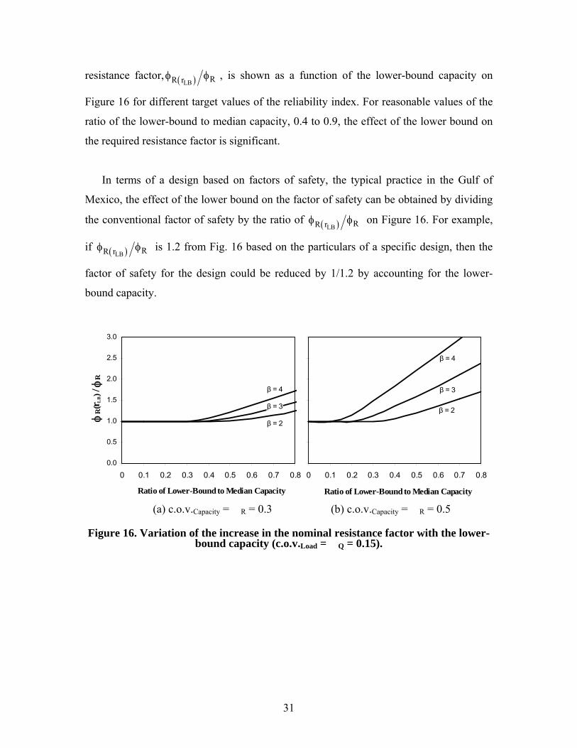
resistance factor, ( )LB RR rφ φ , is shown as a function of the lower-bound capacity on

Figure 16 for different target values of the reliability index. For reasonable values of the

ratio of the lower-bound to median capacity, 0.4 to 0.9, the effect of the lower bound on

the required resistance factor is significant.

In terms of a design based on factors of safety, the typical practice in the Gulf of

Mexico, the effect of the lower bound on the factor of safety can be obtained by dividing

the conventional factor of safety by the ratio of ( )LB RR rφ φ on Figure 16. For example,

if ( )LB RR rφ φ is 1.2 from Fig. 16 based on the particulars of a specific design, then the

factor of safety for the design could be reduced by 1/1.2 by accounting for the lower-

bound capacity.

0.0

0.5

1.0

1.5

2.0

2.5

3.0

0 0.1 0.2 0.3 0.4 0.5 0.6 0.7 0.8


Req

uire

d M

edia

n F

acto

r of

Saf

ety

β = 4

β = 3

β = 2

0.0

0.5

1.0

1.5

2.0

2.5

3.0

0 0.1 0.2 0.3 0.4 0.5 0.6 0.7 0.8


β = 4

β = 2

β = 3

φR

(r LB) /

φR

(a) c.o.v.Capacity = �R = 0.3 (b) c.o.v.Capacity = �R = 0.5

Figure 16. Variation of the increase in the nominal resistance factor with the lower-bound capacity (c.o.v.Load = �Q = 0.15).

31

Added Design Checking Equation for Lower-Bound Capacity An alternative code format would be to have two design checking equations:

(7)

LB

R nomin al Q nomin al

R LB Q nomin al

r q

ORr q

φ ≥ γ

φ ≥ γ

where the first design checking equation is the conventional equation and the second

equation includes a resistance factor, LBRφ , that is applied directly to the lower-bound

capacity. Providing that one or the other of the two equations is satisfied, a design will

provide the specified level of reliability. The motivation for this form of the design

checking equation is that the conventional approach is incorporated and does not need to

be modified, whether or not there is a lower-bound capacity; the effect of a lower-bound

capacity is reflected entirely in the second equation.

A plot of versus the lower-bound capacity is shown on Figure 17 for different

target reliability indices. The curves begin at values of the lower-bound capacity,

specifically

LBRφ

LB medianr r , where the second design checking equation in Equation (7)

governs. One advantage of this approach with two design checking equations (Equation 7

versus Equation 6) is that is not very sensitive to either the magnitude of the lower-

bound capacity or the target reliability index (Fig. 17). In fact, a conservative value of

around 0.75 for could be used to cover a wide range of possibilities.

LBRφ

LBRφ

32

0.0

0.2

0.4

0.6

0.8

1.0

1.2

1.4

0 0.1 0.2 0.3 0.4 0.5 0.6 0.7 0.8 0.9 1


Req

uire

d M

edia

n F

acto

r o

f Sa

fety

ß = 4

ß = 3

ß = 2

0.0

0.2

0.4

0.6

0.8

1.0

1.2

1.4

0 0.1 0.2 0.3 0.4 0.5 0.6 0.7 0.8 0.9 1


ß = 2

ß = 3

ß = 4

Low

er B

ound

Res

ista

nce

Fact

or, φ

RL

B

(a) c.o.v.Capacity = �R = 0.3 (b) c.o.v.Capacity = �R = 0.5

Figure 17. Variation of the lower-bound resistance factor to account for a lower-bound capacity (c.o.v.Load = �Q = 0.15).

Value of Site Characterization and Installation Data

By considering all of the factors together in the design of a suction caisson, the

relative importance of site characterization information can be assessed. In terms of

capacity, the consequence of not having site-specific borings at every caisson location is

relatively small. At most, the total c.o.v. in capacity would be reduced by about 80

percent (if the c.o.v. in the design method is 0.25 and the c.o.v. due to spatial variability

is 0.2). However, when the load uncertainty, the effect of a lower-bound value on the

caisson capacity, and the factors of safety are included, this reduction in uncertainty

would be negligible for conventional design practice. Another way to say this is that the

reliability that is being achieved in design practice is so high (Figs. 10 and 15) that there

is plenty of room for relatively small variations in soil properties without impacting the

reliability. However, site characterization data can play a much more significant role in

foundation installation, which has not been addressed in this research.

On the other hand, the presence of a lower-bound value on the capacity can have a

significant effect on the reliability (Fig. 14). Data on the lower-bound capacity can be

obtained from caisson installation. Therefore, there is a significant potential to make

designs more efficient and effective by making use of installation data to verify and

33

update estimates of capacity. While outside the scope of this research, this approach

would be particularly useful for Mobile Offshore Drilling Units.

Summary Major conclusions from this work as follows:

1. The magnitude of spatial variability in the capacity of suction caissons depends

substantially on the geologic setting. In normally consolidated marine clays in

deepwater in the Gulf of Mexico, the absolute variability is small with

coefficients of variation between 0.1 and 0.2. While small in an absolute sense,

the magnitude of spatial variability in the capacity of suction caissons is greater

than that for driven piles due to the effects of spatial averaging over the long

length of a driven pile.

2. The uncertainty in design models for suction caissons is comparable to but

slightly higher than that for driven piles in normally consolidated clays.

3. There is a physical lower-bound to the range of possible capacities, and this

lower-bound can have a significant affect on the reliability of the foundation. One

practical implication of this effect is to include a design check using the lower-

bound capacity in addition to the nominal or design capacity. A second practical

implication is that installation data can be used to update the reliability even when

significant set-up is expected

4. Foundation designs for permanent floating production systems may be

excessively conservative. The probability of failure values being achieved are

several orders of magnitude smaller than industry-recommended targets for

components (single line or foundation) in a mooring system. The practical

concern with such excessive conservatism is that installation can become

unnecessarily costly and problematic. In fact, if one suction caisson in the

mooring spread cannot be installed, then the risk actually increases because the

system is in a damaged state from the start.

34

5. The practice of not having geotechnical borings or probes at the location of every

suction caisson in a facility layout does not adversely impact the reliability of the

foundation because the effects of this uncertainty are negligible in light of the

uncertainties in the loads, the presence of a lower-bound on the capacity, and the

design factors of safety that are used today in practice.

35

References Aubeny, C. P., Han, S., and Murff, J. D. (2003). Refined model for inclined load capacity

of suction caissons. Proceedings of the International Conference on Offshore Mechanics and Arctic Engineering, OMAE, pages-5.

American Petroleum Institute: Recommended Practice for Planning Designing, and constructing Fixed Platforms-Load and Resistance Factor Design, RP 2A-LRDF, Washington D.C., 1993.

Banon, H. and Hardin, S. J. 1989. Methodology for Assessing Reliability of Tension Leg Platform Tethers. Journal of Structural Engineering, Vol. 115, No. 9: 2243 – 2259.

Bea, R. G., Jin, Z., Valle, C. and Ramos, R. 1999. Evaluation of Reliability of Platform Pile Foundations. J. Geotech. and Geoenvir. Engrg., ASCE, 125(8): 696-704.

Chen, W. and Randolph, M. F. (2005), “Centrifuge Tests on Axial Capacity of Suction Caissons in Clay,” Proceedings of International Symposium on Frontiers in Offshore Geotechnics: ISFOG 2005, Perth, Australia.

Cho, Y., Lee, T. H., Chung, E. S., and Bang, S. (2003). Field tests on pullout loading capacity of suction piles in clay. Proceedings of the International Conference on Offshore Mechanics and Arctic Engineering, OMAE, pages-7.

Clukey, E. C. (2001). Suction caisson design issues. Proceedings of the OTRC International Conference, 163-181.

Clukey, E. C., Aubeny, C. P., and Murff, J. D. (2003). Comparison of analytical and centrifuge model tests for suction caissons subjected to combined loads. Proceedings of the International Conference on Offshore Mechanics and Arctic Engineering, OMAE, pages-6.

Clukey, E. C., Banon, H. and Kulhawy, F. H. 2000. Reliability Assessment of Deepwater Suction Caissons. Proc. Offshore Technology Conf., Houston, OTC 12192: 777-785.

Clukey, E. C. and Morrison, M. J. (1993). A centrifuge and analytical study to evaluate suction caissons for TLP applications in the Gulf of Mexico. Geotechnical Special Publication No. 38, ASCE, 141-156.

Clukey, E. C. and Phillips, R. (2002). Centrifuge model tests to verify suction caisson capacities for taut and semi-taut legged mooring systems. Proceedings, International Conference on Deepwater Offshore Technology.

Dangayach, S. 2004. Reliability Analysis of Mooring System for Spar. M. S. Thesis, University of Texas at Austin: 84 pp.

Ding, Y., Kim, M., Chen, X. and Zhang, J. 2003. Coupled Analysis of Floating Production System. Proc. Intern. Symp. on Deepwater Mooring Systems, Concepts, Design, Analysis, and Materials, Houston, Texas: 152-167.

El-Sherbiny, Rami M. (2005), “Performance of Suction Caisson Anchors in Normally Consolidated Clay”, Ph.D. dissertation, University of Texas, Austin, August.

Gilbert, R. B. and Murff, J. D. (2001), “Identifying Uncertainties in the Design of Suction Caisson Foundations,” Proceedings, International Conference on Geotechnical, Geological and Geophysical Properties of Deepwater Sediments Honoring Wayne A. Dunlap, OTRC, Houston, Texas, 231-242.

Gilbert, R. B. (2003), “Reliability-Based Design as a Decision-Making Tool,” Proceedings, International Workshop on Limit State Design in Geotechnical Engineering Practice, Phoon, Honjo and Gilbert (eds.), Cambridge, Massachusetts.

36

Gilbert, R. B., Najjar, S. S., Choi, Y. J. (2005). Incorporating lower-bound capacities into LRFD codes for pile foundations. Proceedings, GeoFrontiers Conference, ASCE, inpress.

Goodwin, P., Ahilan, R. V., Kavanagh, K. and Connaire, A. 2000. Integrated Mooring and Riser Design: Target Reliabilities and Safety Factors. Proc. of OMAE: 185-792.

Hamilton, J. M. and Murff, J. D. 1992. Selection of LRFD Resistance Factors for Pile Foundation Design. Proc. of Structural Congress ’92, ASCE, San Antonio, Texas: 788-795.

Horsnell, M. R. and Toolan, F. E. .1996. Risk of Foundation Failure of Offshore Jacket Piles. Proc. of Offshore Tech. Conf., OTC 7997: 381-392.

House, A. R., and Randolph, M. F. (2001). Installation and pullout capacity of stiffened suction caissons in cohesive sediments. Proceedings, 11th International Offshore and Polar Engineering Conference.

Jeanjean, P. Znidarcic, D., Phillips, R. Ko, H.Y., Pfister, S., Cinicioglu, O. and Schroeder, K. (2006), “Centrtifuge Testing on Suction Anshors: Double-Wall, Overconsolidated Clay, and Layered Soil Profile,” Proceedings, Offshore Technology Conference, OTC 18007.

Luke, A. M., Rauch, A. F., Olson, R. E., and Mecham, E. C. (2003). Behavior of suction caissons measured in laboratory pullout tests. Proceedings of the International Conference on Offshore Mechanics and Arctic Engineering, OMAE, pages-9.

Murff, J. D. and Hamilton, J. M. (1993). P-Ultimate for undrained analysis of laterally loaded piles. Journal of Geotechnical Engineering, ASCE, Vol. 119, No. 1, 91-107.

Najjar, S. S. (2005), “Importance of Lower-Bound Capacities in Geotechnical Reliability Assessments,” Ph.D. Dissertation, The University of Texas at Austin: 317 pp.

Neubecker, S. R. and Randolph, M. F. 1995. Performance of Embedded Anchor Chains and Consequences for Anchor Design. Proc. Offshore Technology Conf., OTC 7712, Houston, Texas: 191-200.

Randolph, M. F., and House, A. R. (2002). Analysis of suction caisson capacity in clay. Proceedings, Offshore Technology Conference, OTC 14236.

Ronold, K. O. 1990. Reliability Analysis of Tension Pile. Journal of Geotech. Engineering, Vol. 116, No. 5: 760-773.

Smith, G. L. and Gilbert, R. B. (2001), “A Simplified Model of Spatial Variability to Evaluate Effects of Spatial Averaging on Foundation Capacity,” Proceedings, International Conference on Structural Safety and Reliability, Huntington Beach, California.

Tang, W. H. 1990. Performance Reliability of Offshore Piles. Proc. of Offshore Tech. Conf., OTC 6379: 299-308.

Tang, W. H. and Gilbert, R. B. 1993. Case Study of Offshore Pile System Reliability. Proc. of Offshore Tech. Conf., OTC 7196: 677-686.

Watson, P. G., Suemasa, N., and Randolph, M. F. (2000). Evaluating Undrained Shear Strength Using the Vane Shear Apparatus. Proceedings, 10th International Offshore and Polar Engineering Conference, 485-493.

Winterstein, S. R. and Kumar, S. 1995. Reliability of Floating Structures: Extreme Response and Load Factor Design, Proc. Offshore Technology Conf., OTC 7758, Houston, Texas: 569-578.

37

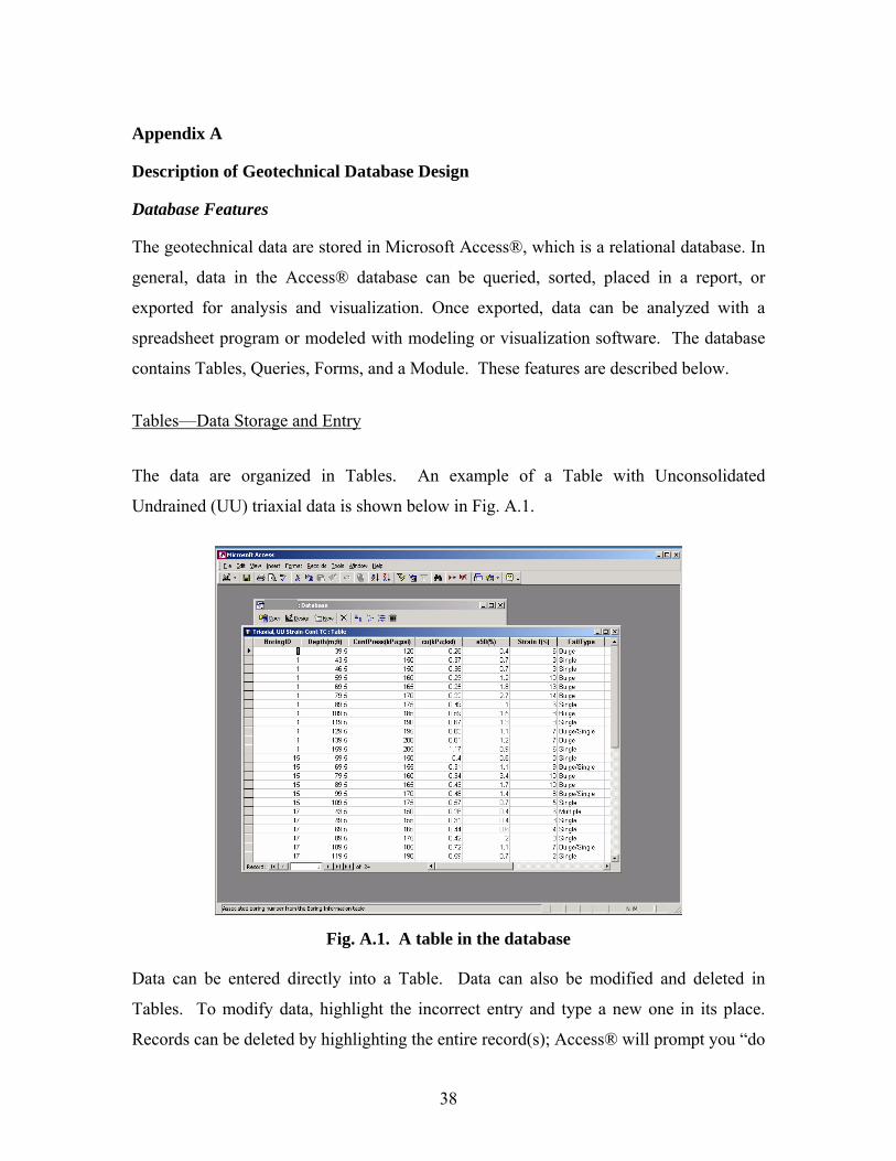
Appendix A

Description of Geotechnical Database Design

Database Features

The geotechnical data are stored in Microsoft Access®, which is a relational database. In

general, data in the Access® database can be queried, sorted, placed in a report, or

exported for analysis and visualization. Once exported, data can be analyzed with a

spreadsheet program or modeled with modeling or visualization software. The database

contains Tables, Queries, Forms, and a Module. These features are described below.

Tables—Data Storage and Entry

The data are organized in Tables. An example of a Table with Unconsolidated

Undrained (UU) triaxial data is shown below in Fig. A.1.

Fig. A.1. A table in the database Data can be entered directly into a Table. Data can also be modified and deleted in

Tables. To modify data, highlight the incorrect entry and type a new one in its place.

Records can be deleted by highlighting the entire record(s); Access® will prompt you “do

38

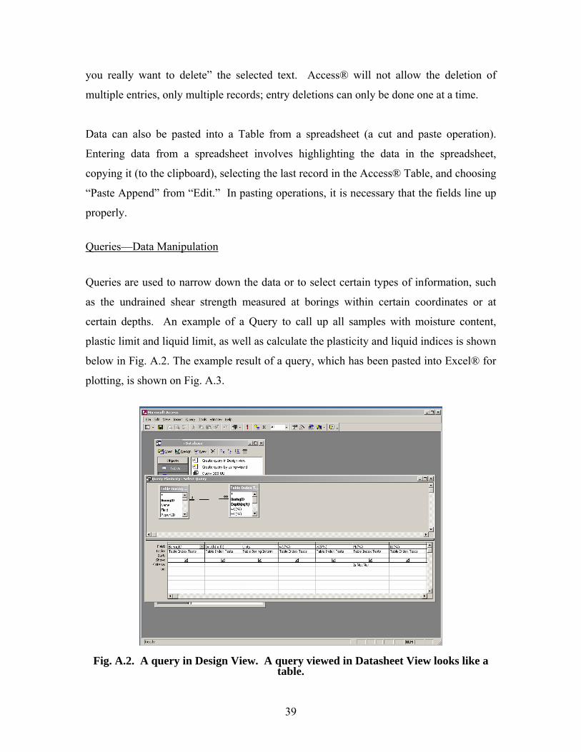
you really want to delete” the selected text. Access® will not allow the deletion of

multiple entries, only multiple records; entry deletions can only be done one at a time.

Data can also be pasted into a Table from a spreadsheet (a cut and paste operation).

Entering data from a spreadsheet involves highlighting the data in the spreadsheet,

copying it (to the clipboard), selecting the last record in the Access® Table, and choosing

“Paste Append” from “Edit.” In pasting operations, it is necessary that the fields line up

properly.

Queries—Data Manipulation

Queries are used to narrow down the data or to select certain types of information, such

as the undrained shear strength measured at borings within certain coordinates or at

certain depths. An example of a Query to call up all samples with moisture content,

plastic limit and liquid limit, as well as calculate the plasticity and liquid indices is shown

below in Fig. A.2. The example result of a query, which has been pasted into Excel® for

plotting, is shown on Fig. A.3.

Fig. A.2. A query in Design View. A query viewed in Datasheet View looks like a table.

39

Fig. A.3. Data from the Query is pasted into Excel to be plotted and analyzed.

Queries can get information from Tables or other Queries. For example, the data can be

further defined by querying a Query. The data can also be modified through Queries.

For example, if an error is detected during a Query it can be corrected in the Query and

will be reflected in the Table and other Queries that contain that data.

Query design is generally a point and click operation with logical operators used to

narrow down a selection. Access® provides an “expression builder” when the user right

clicks in the “criteria” field of the Query design screen. For non-routine Queries, the on-

line help is useful.

Forms—Automation

Forms are used to make using the database more convenient. For example, they may be

used to automate common processes, or display data from a Table in a way more pleasing

to the eye. A Form is based upon one or more Tables or Queries. The data in a Form

may be displayed in datasheet mode (looks like a Table) or in standard form mode.

Standard form mode shows only one record at a time. You can toggle between the two

40

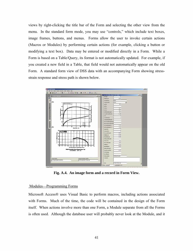
views by right-clicking the title bar of the Form and selecting the other view from the

menu. In the standard form mode, you may use “controls,” which include text boxes,

image frames, buttons, and menus. Forms allow the user to invoke certain actions

(Macros or Modules) by performing certain actions (for example, clicking a button or

modifying a text box). Data may be entered or modified directly in a Form. While a

Form is based on a Table/Query, its format is not automatically updated. For example, if

you created a new field in a Table, that field would not automatically appear on the old

Form. A standard form view of DSS data with an accompanying Form showing stress-

strain response and stress path is shown below.

Fig. A.4. An image form and a record in Form View.

Modules—Programming Forms

Microsoft Access® uses Visual Basic to perform macros, including actions associated

with Forms. Much of the time, the code will be contained in the design of the Form

itself. When actions involve more than one Form, a Module separate from all the Forms

is often used. Although the database user will probably never look at the Module, and it

41

contains no data from the database, it is important that it exists and functions so features

associated with Forms will function properly.

Database Structure

The database allows data entry and manipulation in three ways: Tables, Queries, and

Forms. Tables contain raw data. Queries may filter, calculate, or join data from Tables

or other Queries. Forms may display the data from a Table or Query in a more

meaningful way and may employ Modules to do it. In this section, the Tables, Queries,

Forms, and Modules included with this database are summarized.

Data Tables The data are organized into 26 Tables. A list of these Tables and a description of their

organization is presented below in Table A.1. The data contained in each Table is

generally intuitive. Most Tables contain data from a certain test. Shear strength tests

with several parameters each have a unique Table. Tests with many inputs or outputs

have a unique Table. Shear strength tests with only 1 or 2 parameters appear together in

the Simple Strength Tests Table. Generally, other tests with only a boring number, a

sample/test depth, and one output are grouped in the Index Tests Table. Images that

apply to a group of tests or the entire boring are recorded in the Images Advanced Tests,

Images Summary, and Images Xray Tables: Note that Tables only contain the image file

names and cannot be used to view the images; to view the images, the associated Form

must be used.

42

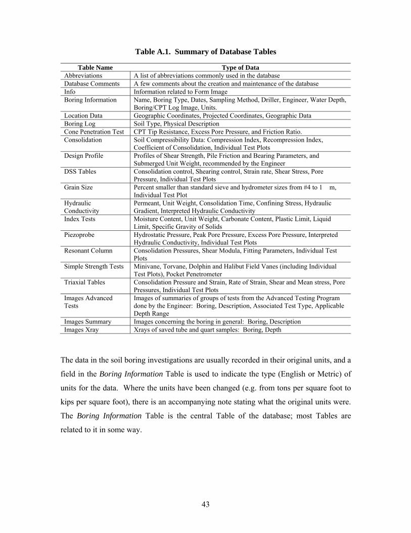
Table A.1. Summary of Database Tables

Table Name Type of Data Abbreviations A list of abbreviations commonly used in the database Database Comments A few comments about the creation and maintenance of the database Info Information related to Form Image Boring Information Name, Boring Type, Dates, Sampling Method, Driller, Engineer, Water Depth,

Boring/CPT Log Image, Units. Location Data Geographic Coordinates, Projected Coordinates, Geographic Data Boring Log Soil Type, Physical Description Cone Penetration Test CPT Tip Resistance, Excess Pore Pressure, and Friction Ratio. Consolidation Soil Compressibility Data: Compression Index, Recompression Index,

Coefficient of Consolidation, Individual Test Plots Design Profile Profiles of Shear Strength, Pile Friction and Bearing Parameters, and

Submerged Unit Weight, recommended by the Engineer DSS Tables Consolidation control, Shearing control, Strain rate, Shear Stress, Pore

Pressure, Individual Test Plots Grain Size Percent smaller than standard sieve and hydrometer sizes from #4 to 1 �m,

Individual Test Plot Hydraulic Conductivity

Permeant, Unit Weight, Consolidation Time, Confining Stress, Hydraulic Gradient, Interpreted Hydraulic Conductivity

Index Tests Moisture Content, Unit Weight, Carbonate Content, Plastic Limit, Liquid Limit, Specific Gravity of Solids

Piezoprobe Hydrostatic Pressure, Peak Pore Pressure, Excess Pore Pressure, Interpreted Hydraulic Conductivity, Individual Test Plots

Resonant Column Consolidation Pressures, Shear Modula, Fitting Parameters, Individual Test Plots

Simple Strength Tests Minivane, Torvane, Dolphin and Halibut Field Vanes (including Individual Test Plots), Pocket Penetrometer

Triaxial Tables Consolidation Pressure and Strain, Rate of Strain, Shear and Mean stress, Pore Pressures, Individual Test Plots

Images Advanced Tests

Images of summaries of groups of tests from the Advanced Testing Program done by the Engineer: Boring, Description, Associated Test Type, Applicable Depth Range

Images Summary Images concerning the boring in general: Boring, Description Images Xray Xrays of saved tube and quart samples: Boring, Depth

The data in the soil boring investigations are usually recorded in their original units, and a

field in the Boring Information Table is used to indicate the type (English or Metric) of

units for the data. Where the units have been changed (e.g. from tons per square foot to

kips per square foot), there is an accompanying note stating what the original units were.

The Boring Information Table is the central Table of the database; most Tables are

related to it in some way.

43

Boring Information

Primary information for each boring is stored in the Boring Information Table. This is

unique information for each boring and requires one record per boring. This information

includes a boring identification number, the area or field where it was drilled, report

numbers, dates, engineer, driller, water depth, boring method, sampling method, final

depth, images of the boring/CPT logs, and type of units used (English or Metric). The

numerical location data—geographic coordinates and projected coordinates (e.g. UTM

coordinates) and their respective geographic data—are contained in the Location Data

Table. Other applicable images (such as design profiles, plasticity profiles, and location

map) may be found in the Images Summary Table.

Index Properties

Two Tables are used to store records based on index property tests. These data include

Atterberg limits, weight-volume information, and grain size. Plastic and liquid limit test

results at a given depth for each boring are listed in the Index Tests Table. This Table

also includes weight-volume information, such as water content, unit weight, carbonate

content, and specific gravity of solids. The Grain Size Table stores the measured percent

passing the United States Standard (USS) sieve numbers 4 and 200 and the ASTM

standard hydrometer sizes 5 �m and 1 �m. The values reported as fines, or silts and

clays are defined as the percent passing the number USS 200 sieve or grain sizes less than

75 �m. Both Tables include Boring ID and Depth to uniquely identify each test and to

link it to the proper boring in the Boring Information Table. Summary plots of these tests

may be found in the Images Summary Table.

Laboratory Engineering Properties

Lab-measured engineering properties are stored in Tables according to the test type. The

data include consolidation, direct simple shear (DSS), hydraulic conductivity, minivane,

torvane, pocket penetrometer, resonant column, and triaxial measurements. Each test is

identified by depth and boring number from the Boring Information Table.

44

Many tests include an image file in the Table. Summary images for tests that were part

of the Advanced Testing Program (Cyclic DSS and Triaxial tests, Stress and Strain

Controlled Triaxial tests--not including UU Tests, Stress Controlled DSS Tests, Resonant

Column Tests, and some Strain Controlled DSS Tests) may be found in the Images

Advanced Tests Table. These may include plots such as strain vs. shear stress and log of

time, or cyclic stress ratio vs. number of cycles. Saved sample X-rays are found on the

Images Xray Table. Other summary images not applying exclusively to the Advanced

Testing Program may be found in the Images Summary Table.

So far, the database contains data from undrained strength tests only. Minivane, Torvane,

and Pocket Penetrometer results are given in the Simple Strength Tests Table. Complex

test results are given in the DSS, Triaxial, and Resonant Column Tables. Each of them

contains index properties measured during or after the test (the initial index properties are

recorded in the Index Properties Table). They also contain consolidation and rate of

strain data.

There are three Tables for different direct simple shear tests. All of them include image

files. The DSS Static, Strain-Cont Table contains strains, stresses, and pore pressures at

peak horizontal shear stress and at high strain. The DSS Static, Stress-Cont Table

contains data pertinent to a creep test, such as loading stress and time increments, applied

stress, and a few time-strain pairs. The DSS Cyclic, Stress-Cont Table contains data for

cyclic shear stress controlled tests. The data include ambient shear strain, average cyclic

shear stress, cyclic shear stress amplitude, and some pairs of number of cycles vs.

average shear strain and vs. cyclic shear strain.

There are five Tables for different triaxial shear tests. All of them include image files.

The Triaxial, UU Strain-Cont TC Table contains data from unconsolidated, undrained,

strain-controlled triaxial compression tests, including confining pressure, undrained shear

strength, failure strain, rate of strain, and mode of failure. The Triaxial, Strain-Cont TC

and Triaxial, Strain-Cont TE Tables contain data for consolidated, undrained, strain-

45

controlled compression and extension tests, respectively. The Tables record K0 where

applicable, as well as strain rate, mean and shear stress, principal stress ratio, pore

pressures, and mode of failure. Consolidated undrained triaxial compression creep test

results are recorded in the Triaxial, Stress-Cont TC Table, and loading stress and time

increments are given, as well as shear strain vs. time pairs and a reference undrained

shear strength. The Triaxial, Stress-Cont Cyclic Table contains data from consolidated

undrained stress-controlled cyclic triaxial tests. Frequency and amplitude of the load are

recorded, along with vertical and horizontal consolidation pressures, and some pairs of

number of cycles vs. average shear strain and vs. cyclic shear strain.

The Resonant Column Table contains consolidation pressure and maximum shear

modulus for each stage, as well as empirical parameters for fitting maximum shear

modulus vs. consolidation pressure, as well as image files.

The Consolidation Table stores the maximum previous consolidation pressure,

constrained modulus for each increment, coefficient of consolidation, and the

overconsolidation ratio, as well as image files.

The Hydraulic Conductivity Table contains test parameters before, during, and after the

test. These data include void ratio, consolidation pressure, hydraulic gradient, permeant,

specimen orientation (horizontal vs. vertical permeability), water content, and hydraulic

conductivity. There are no individual test plots.

Field Engineering Properties

Field measured soil properties are recorded in three Tables, which uniquely identify each

data point by its Boring identification number and depth. These Tables are Cone

Penetration Test, Piezoprobe, and Simple Strength Tests.

The Cone Penetration Test Table stores point data entered for continuous CPT data. The

data consist of cone resistance, pore water pressure, and friction ratio as a function of

46

depth. Entered point data vary from 0.5 to 2 feet (0.2 to 0.5 meters) of depth, depending

on the resolution required to reflect the variability of the cone measurements. The image

of the CPT log may be found on the Boring Information Table.

The Piezoprobe Table contains pore pressure data measured in the field, including

hydrostatic pressure, peak pore pressure, estimated pore pressure, excess pore pressure,

and hydraulic conductivity. Plots are included.

Dolphin and Halibut field vane test results are found in the Simple Strength Tests Table.

The information includes the blade size and the measured in-situ and remolded shear

strengths. Images are included.

Design Information

Design information is recorded in two Tables. The Boring Log Table stores the soil

descriptions as interpreted from the boring logs by the engineers. This Table, which is

linked to the Boring Information Table, includes the depth intervals and description of

each soil stratum. The description generally gives information about density, gradation,

strength, and color; for example “Gray medium dense fine sand’ or “Stiff gray clay”. An

image of the boring log may be found on the Boring Information Table.

The Design Profile Table includes the design parameters for axial and lateral pile

capacity as interpreted by the engineers based on measured values. These data include

design undrained shear strength, design friction angle, and submerged unit weight, the

strain at 50 percent deviator stress in a triaxial undrained test, and subgrade modulus.

Design profile plots may be found in the Images Summary Table.

Supplemental Information

Some supplemental information is recorded in two Tables. The Abbreviations Table

gives a list of abbreviations used elsewhere in the database. The Database Comments

47

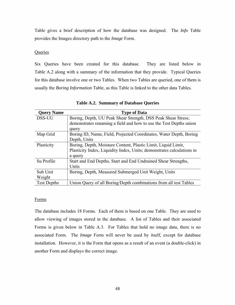
Table gives a brief description of how the database was designed. The Info Table

provides the Images directory path to the Image Form.

Queries Six Queries have been created for this database. They are listed below in

Table A.2 along with a summary of the information that they provide. Typical Queries

for this database involve one or two Tables. When two Tables are queried, one of them is

usually the Boring Information Table, as this Table is linked to the other data Tables.

Table A.2. Summary of Database Queries

Query Name Type of Data

DSS-UU Boring, Depth, UU Peak Shear Strength, DSS Peak Shear Stress; demonstrates renaming a field and how to use the Test Depths union query

Map Grid Boring ID, Name, Field, Projected Coordinates, Water Depth, Boring Depth, Units

Plasticity Boring, Depth, Moisture Content, Plastic Limit, Liquid Limit, Plasticity Index, Liquidity Index, Units; demonstrates calculations in a query

Su Profile Start and End Depths, Start and End Undrained Shear Strengths, Units

Sub Unit Weight

Boring, Depth, Measured Submerged Unit Weight, Units

Test Depths Union Query of all Boring/Depth combinations from all test Tables

Forms The database includes 18 Forms. Each of them is based on one Table. They are used to

allow viewing of images stored in the database. A list of Tables and their associated

Forms is given below in Table A.3. For Tables that hold no image data, there is no

associated Form. The Image Form will never be used by itself, except for database

installation. However, it is the Form that opens as a result of an event (a double-click) in

another Form and displays the correct image.

48

To view an image is simple: Just double-click on the name of the file. A new Image

Form will open and the image will be displayed. The path to the Images directory is

shown below and to the left of the image, while the path and filename relative to that

directory is shown below and to the right of the image. The file name appears in the title

bar. Multiple Image Forms may be open at once. Each one can be closed separately.

Table A.3. Tables and their Associated Forms

Table Name Associated Form Name

Abbreviations --

Boring Information Boring Information Boring Log -- Cone Penetration Test -- Consolidation Consolidation Database Comments -- Design Profile -- DSS Cyclic, Stress-Cont DSS Cyclic, Stress-Cont DSS Static, Strain-Cont DSS Static, Strain-Cont DSS Static, Stress-Cont DSS Static, Stress-Cont Grain Size Grain Size Hydraulic Conductivity -- Images Advanced Tests Images Advanced Tests Images Summary Images Summary Images Xray Images Xray Index Tests -- Info Image Location Data -- Piezoprobe Piezoprobe Resonant Column Resonant Column Simple Strength Tests Simple Strength Tests Triaxial, Strain-Cont TC Triaxial, Strain-Cont TC Triaxial, Strain-Cont TE Triaxial, Strain-Cont TE Triaxial, Stress-Cont Cyclic Triaxial, Stress-Cont Cyclic Triaxial, Stress-Cont TC Triaxial, Stress-Cont TC Triaxial, UU Strain-Cont TC Triaxial, UU Strain-Cont TC

Modules The database includes one Module called basPublic. It is used by all of the Forms to

open a new Image Form and to maintain the Image Forms while they are open.

49

Documents

Suction Caissons: Seafloor Characterization for Deepwater