Sugar Policy Reform, Tax Policy and Price

Transmission in the Soft Drink Industry.

C. Bonnet and V. Réquillart

 

 

Working Paper No. 4 

Transparency of Food Pricing 

TRANSFOP 

 

Seventh Framework Programme Grant Agreement No. KBBE­265601­4­TRANSFOP 

                                                                            

                                        

 

Sugar Policy Reform, Tax Policy and Price Transmission in theSoft Drink Industry.

Céline Bonnet� and Vincent Requillarty

January 2012z

Abstract

There is growing interest in evaluating the impact of price variations in agricultural commoditieson food prices and consumption. Food industries typically consist of large �rms that bene�t frommarket power and price transmission along the chain is a¤ected by this imperfectly competitiveenvironment. In this paper, we propose an empirical analysis of the impact of a reform of the EUsugar policy on the soft drink industry. The reform produces a signi�cant decrease in the price ofsugar. We consider how the manufacturers and the retailers both strategically react to this changein the production cost of soft drinks. Using a structural econometric model, we �rst estimate theconsumer substitution patterns and the models for the vertical relationships between the soft drinkindustry and the retail industry. After selecting the �best�model for vertical relationships, we simulatethe impact of the sugar policy reform. We show that the retail prices decrease more than the marginalproduction costs. Our results thus suggest that the assumption of passive pricing by the industryleads to a poor estimate of the impact of an upstream cost shock. We also simulate the impact of arecently enacted excise tax on soft drinks. Because of strategic pricing, this tax is likely to lead toan increase of approximately 10% in prices thereby decreasing the soft drink consumption by morethan 3 liters per person per year.

JEL codes:H32, L13, Q18, I18

Key words: vertical contracts, two-part tari¤s, competition, manufacturers, private labels, re-tailers, di¤erentiated products, soft drinks, non-nested tests, sugar policy, pass-through.

�Toulouse School of Economics (INRA, GREMAQ), 21 Allée de Brienne, F-31000 Toulouse France, Tel: +33 (0)5 61 1285 91, cbonnet@toulouse.inra.fr

yToulouse School of Economics (INRA, GREMAQ; IDEI), 21 Allée de Brienne, F-31000 Toulouse France, Tel: +33 (0)561 12 86 07, vincent.requillart@toulouse.inra.fr

zThis paper is part of the �Transparency of Food Pricing� (TRANSFOP) project funded by the European Commis-sion, Directorate General Research - Unit E Biotechnologies, Agriculture, Food. Grant Agreement No. KBBE-265601-4-TRANSFOP. We thank Marine Spiteri for her help to collect some information of sugar content in the Soft Drink Industry.We also thank participants at the ALISS-INRA seminar, the internal IFS seminar at London, the Nineteenth EuropeanWorkshop on Econometrics and Health Economics in Lausanne, the �rst joined EAAE/AAEA seminar in Freising and theINRA-SFER-CIRAD conference in Dijon. Any remaining errors are ours.

1

1 Introduction

Even in developed countries a signi�cant portion of the population is extremely concerned about food

price in�ation. On average, in the EU27, food expenditure accounts for 22.2% of the total expenditures

of the consumers in the �rst quintile of income. There is an even larger proportion of 30% seen in eight

EU27 countries. Consumers in the third quintile of income devotes 14%, 19.1% and 25.2% of their total

expenditures to food in France, Spain and Hungary, respectively (Eurostat data).

Following the peak of agricultural commodity prices in 2007-2008, the food price in�ation in the EU has

shown considerable discrepancy across countries (Bukeviciute et al., 2009). For example, from July 2007

to August 2008, the consumer food price index increased by less than 4% in France while simultaneously

rising by over 6% in Austria, Denmark, Ireland and the UK and over in Hungary. According to these

authors, the elasticity of consumer food prices to producer food prices was approximately 25% in the

UK, which was larger than the 30% observed in Sweden, and lower than the 15% observed in Romania

or the 15 - 20% observed in the Eurozone on average. The speed of adjustment in the consumer price

to a change in the producer price is also quite variable. Although the price transmission of food prices

along the food chain is relatively well documented through time-series analysis (e.g. Vavra and Goodwin,

2005), the main determinants of food price transmission remain unclear. Few structural analyses have

addressed the functioning of the food chain and its implications in term of price transmission. OECD

(2011) expects that over the coming decade the real prices for many agricultural products could increase

by 20% to 30% higher compared with the prices in 2001-2010. Furthermore, increased volatility in the

prices is forecasted. Therefore, the explanations of the transmission of price variations is of increasing

interest.

Food chains typically consist of large �rms with market power. Many food categories are highly

concentrated: the concentration ratio for the top four industries is above 50%. For instance, the con-

centration ratio for the top four ice cream producers was over 58%, that in the soft drinks category was

64% and that in the savory biscuits category was 68% in Europe in 2001 (Bukeviciute et al., 2009). At

2

the retail level, because of the concentration process of recent decades, the top �ve supermarket retailers

now account for over 50% of the groceries market in many EU countries. This consolidation process

could impact the balance of power between food producers and retailers. We are then faced with an

imperfectly competitive environment in food chains. The theoretical literature that explores price trans-

mission in this context is limited. Carbonnier (2006) shows that under a Cournot competition, the cost

pass-through might be less than or greater than 100% and particularly depends on the curvature of the

demand curve.1 Anderson et al. (2001) investigated price transmission in a Bertrand competition with

di¤erentiated products. The empirical literature has more examples. Note that in this literature, the

pass-through rates are frequently reported in the elasticity form rather than as a level. As soon as there

is a wedge between the price and the marginal cost in the market the pass-through in the elasticity form

becomes lower than the pass-through as a level. For example, Nakamura and Zerom (2010) studied the

US co¤ee industry and reported a long-run pass-through of co¤ee commodity prices to retail prices of

0.252 in elasticity form and 0.916 in level form. Interestingly, they showed that the markup adjustment

explained a signi�cant part of the incomplete pass-through in this market. Bettendorf and Verboven

(2000) reached a similar conclusion in their analysis of the co¤ee market in Europe. Hellerstein (2008)

showed that the markup adjustment at the manufacturer and the retailer levels plays an important role

in explaining the incomplete pass-through of cost changes (arising from changes in the exchange rate)

in the beer industry. In this case, the markup adjustment accounts for approximately half of the ex-

planation for the incomplete pass-through. Overall, these papers suggest that �rms should strategically

adjust their markups when facing a change in their input costs. Kim and Cotterill (2008) suggested that

the pass-through rate is lower under collusive behavior than under more competitive behavior in the US

processed cheese industry. Bonnet et al. (2009) showed that the pass-through rate for upstream cost

shocks in the ground co¤ee category to the downstream retail prices depends on the form of the contracts

between the manufacturers and the retailers. For example, the pass-through rate is 10 percentage points

higher with resale price maintenance than with standard non-linear pricing.

1Following Kim and Cotterill (2008), we assume that the �cost pass-through rate is de�ned as the proportion of a changein input cost that is passed through to the �nal price of the product�.

3

In this paper, we investigate the potential impact on consumer prices of a recent reform of the EU

sugar policy taking into account the markup adjustment of the manufacturers and the retailers. Over

the last 20 years, the sugar price in the European Union (EU) was well above the world market price. A

combination of a price �oor, import duties, export subsidies and quotas was used to sustain the domestic

price (European Commission, 2004). Moreover because of a restrictive quota, high fructose corn syrup

(HFCS) did not substitute for sugar in the EU as it did in the US.2 Thus, in the EU, the price of caloric

sweeteners was higher than that in other countries. In February 2006, a reform of the EU sugar policy

was agreed upon (Union Européenne, 2006). The reference price, which roughly acts as a �oor price, was

reduced by 36% over a 4-year period starting in 2006.

Sugar is used as an input in many food industries. In particular, it is an important input for the soft

drink (SD) industry because the sugar content of SDs ranges from 6% to 11%. Moreover, the sugar costs

range from 7 to 24% of the �nal price of SDs. The anticipated 36% decrease in the price of sugar could

have a signi�cant impact on consumer prices. Our approach is original because it addresses with a vertical

chain that is composed of oligopolies. The SD industry is highly concentrated, as is the retail industry. It

is thus necessary to explicitly address imperfect competition in the chain to analyze how any changes in

input costs are transmitted to the �nal consumers. This paper uses structural econometric models that

accounts for the structure of the industry: in particular the horizontal and vertical interactions between

the manufacturers and the retailers, unlike the pass-through analysis of Kim and Cotterill (2008), which

assumes that manufacturers and retailers are vertically integrated. Using estimates for the consumers�

demand in the French SD market, we recover price cost margins from several supply models as in Berto

Villas-Boas (2007) and Bonnet and Dubois (2010). We then select the model that best �ts the data.

Using this selected model, we quantify the impact of the alternative scenarios on prices, on the market�s

share of the di¤erent SDs and on consumption. We �rst analyze the e¤ects of the EU sugar policy

reform and then address the impact of an excise tax on SDs that was recently voted for by the French

representatives. Our results suggest that the manufacturers and the retailers use two-part tari¤ contracts

2For an analysis of competition between sugar and HFCS in the EU, see Cooper et al. (1995). For an analysis of theUS market, see Beghin et al. (2003).

4

and transmit an amount greater than the cost change to their consumers. The pass-through rate of a cost

change is approximately 1.1. Ignoring the strategic e¤ect then leads to biased estimates of the impact

of the sugar policy reform. As a consequence, the decrease in sugar prices will lead to a decrease in the

consumer price of over 4% for regular SDs, thereby generating a consumption increase greater than 9%

for the regular products, to the detriment of the diet products. The 0.0716 e/liter tax on SDs has a

large impact on both consumer prices and on consumption. In particular, because of strategic pricing,

the tax is over-transmitted to consumers with a pass-through rate of 1.14. When the tax is applied to all

products, the aggregate consumption of soft drinks decreases by approximately 3.4 liters per person per

year which represents roughly 15% of the initial consumption.

This paper is organized as follows. Section 2 presents the main characteristics of the SD industry.

Section 3 presents the data and the descriptive statistics regarding soft drink consumption. Section 4

describes the model and the methods that are used to analyze the demand and to infer the more likely

vertical relationships between manufacturers and retailers. In Section 5, we discuss demand and supply

results and cost estimates. In Section 6, we present the results of the policy simulations and we conclude

this paper in Section 7.

2 The soft drink market

In 2004, the turnover of the French soft drink industry reached 2.2 billion euros, which is 1.6% of the total

turnover of the French food industry. SDs represent approximately 11% of the consumption of beverages

in France which includes mineral water, alcohol, co¤ee, tea, drinking-milk and fruit juices.3 On average,

SD consumption increased by 32% from 1994 to 2004.4 Nevertheless, the per capita consumption in

France (42.5 liters per year) remains lower than that in the EU (71.2 liters on average). Market analysts

frequently distinguish between carbonated soft drinks, or sodas (e.g. colas, tonics, carbonated fruit drinks,

lemonade) and non-carbonated soft drinks (e.g. iced tea, fruits drinks). In France in 2004, carbonated

3Canadean 2004, website http://www.canadean.com/.4Note that the consumption of diet drinks increased by 224% from 1994 to 2004. Nevertheless, the market share is still

below 20%.

5

and non-carbonated SDs represented 78.5% and 21.5% of the market, respectively. The three main

categories of SD are colas (54% of all SDs), fruit drinks (25% for both carbonated and non-carbonated

products) and iced tea (8%). Soft drinks do not include fruit juices and nectars, which represent a

signi�cant portion of beverage consumption. These products do not contain a signi�cant proportion of

added sugar and they are thus not directly a¤ected by the change in sugar price.5 In our analysis, they

are included in the �outside�option for consumers because they are substitutes for SDs.

In general, there are two versions of each SD: a regular version which is sweetened using caloric

sweeteners, mainly sugar in France, and a diet version which is sweetened using non-caloric sweeteners

such as aspartame or acesulfame. The two primary ingredients of regular SDs are water (approximately

90%) and sweetener (approximately 10%). The primary ingredient of a diet soft drink is water (99.7%).

Obviously, soft drinks also contain food additives such as food coloring, arti�cial �avoring, emulsi�ers

and preservatives.

The industry is highly concentrated with the top two manufacturers (the alliance of Coca Cola En-

terprises and Cadbury Schweppes and, the alliance of Unilever and Pepsico) sharing 88.6% of the total

production in 2004. Each of the manufacturers owns a brand portfolio even if Coca Cola and Pepsico are

mainly involved in colas products and Unilever in iced tea. This situation is the result of two mergers:

Coca-Cola Enterprises and Cadbury Schweppes merged their European drink industries in 1999, and

Unilever and Pepsico together created Pepsi Lipton International in 2003.

3 Data

We use consumer panel data collected by TNS WordPanel which is a French representative survey of

19,000 households over a three-year period (2003-2005). This survey provides information on the pur-

chases of food products (quantity, price, brand, characteristics of goods, store). According to our sample,

the average consumption of regular soft drinks is 34 liters per person per year, whereas the average

consumption of diet products is 8 liters per person per year.

5Fruit juices do not contain added sugar whereas nectar contains less than 6% of added sugar.

6

From the panel data, we selected the eleven primary national brands (NB) from the soft drink industry

as well as three private labels (PL), one for each of the three categories of products (colas, iced tea, fruit

drinks). We selected the nine largest retailers in France, which are grocery store chains and di¤er by

the size of their outlets as well as by the services that they provide to consumers. Three of the selected

retailers primarily have large outlets (larger than 2,500 m2) located in suburbs and two primarily have

intermediate-sized outlets (from 400 to 2,500 m2) that are generally located near small cities. Two

retailers have both large and intermediate size outlets. Finally, the last two retailers are discounters with

outlets of small to intermediate size. Taking into account the set of products carried by each retailer we

obtain 105 (or 104, depending on the period) di¤erentiated products that compete on the market.6

Market shares are de�ned as follows. We �rst consider the total market for non-alcoholic beverages

including soft drinks, fruit juice and nectar. This market is considered to be the relevant market. The

market shares of a given brand at a given retailer is de�ned as the ratio of the sum of the quantities of

the brand purchased at the selected retailer during a period of four weeks and the sum of quantities of

all brands purchased at all of the retailers in the relevant market during the same period. The outside

option (which represents 66% of the entire market) is composed of two elements: purchases of fruit juice

and nectar (40% of the market) and purchases of other SDs (77 brands with a very low market share for

a total of 11% of the market) or purchases of the considered SDs at non-considered retailers (66 other

retailers as well as other distribution channels for a total of 16% of the market).

As shown in Table 1, the products selected for our analysis represent 33.8% of the entire market. The

average price over all products and all periods is 0.76 euros per liter. Regular products dominate, as they

represent approximately 80% of the SD purchases; their prices is 15% lower than the price for the diet

products. PLs hold approximately 27% of the SD market and are sold at approximately half of the price

of NBs.

We provide additional information on the SD market (excluding the �outside goods�) in the Annexes

(Tables 6 and 7). Brands 1 to 11 are NBs whereas brands 12 to 14 are PLs. The main NB has a market

6From the consumer perspective, a product is the combination of a brand and a retailer.

7

Table 1: General Descriptive Statistics for Prices and Market Shares.

Prices (in euros per liter) Market SharesMean (std) Mean in %

Outside Good 66.2Soft Drinks 0.76 (0.02) 33.8

Regular products 0.73 (0.02) 80.8Diet products 0.88 (0.03) 19.2National brands 0.89 (0.02) 73.1Private labels 0.40 (0.01) 26.9

share of over 30% (of the soft drink market), whereas the least popular one has less than 1% of the

market. The market share for the private label products varies between 6 and 12%. The average NB

prices vary from 0.74 to 1.12 e/l, whereas PL prices range from 0.38 to 0.54 e/l. The market shares

of the retailers are also heterogenous and vary from 2% to 20%. On average, the prices at the di¤erent

retailers are similar except at retailers 8 and 9, which sell at signi�cantly lower prices because a large

share of their sales is derived from private labels.

4 Models and methods

To analyze strategic pricing in the food chain, we follow a general methodology that was recently developed

to analyze vertical relationships between manufacturers and retailers (e.g. Berto Villas-Boas, 2007; Bonnet

and Dubois, 2010). We consider a demand model to obtain the price elasticities of demand for every

product. The model needs to be as �exible as possible, and we therefore opt for a random coe¢ cients logit

model (Berry et al., 1995; McFadden and Train, 2000). Strategic pricing in the channel can be modi�ed

by the nature of the contracts between the �rms in the sector or by the vertical restraints considered.

We design, as suggested by Bonnet et al. (2009), alternative models for the vertical relationships between

the processors and the retailers. From the �rst-order conditions and estimates of demand, we are able to

calculate the price cost margins for manufacturers and retailers, from which we deduce the cost estimates.

To choose the vertical relationship model that best �ts the data, we �rst estimate a cost model where

8

the calculated cost for each vertical relationship model is the endogenous variable, and we then use a

non-nested Rivers and Vuong (2002) test to select the best model. Finally, using the selected model, we

simulate the impact of the alternative price policies (the reform of the sugar policy and the excise tax on

SDs) on consumers�prices and consumption. In the following, we provide a brief summary regarding the

main assumptions and methods. The reader will �nd more extensive explanations regarding the details

of the method in Bonnet and Dubois (2010).

4.1 The Demand Model: a random coe¢ cients logit model

We use a random coe¢ cients logit model to estimate the demand and the related elasticities. The indirect

utility funtion Vijt for consumer i buying product j in period t is given by

Vijt = �j + t � �ipjt + �ilj +2X

k=1

� ikck(j) + �jt + "ijt

where �j are product �xed e¤ects that capture the (time invariant) unobserved product characteristics,

t are the time �xed e¤ects that capture time demand shocks, pjt is the price of product j in period t,

�i is the marginal disutility of the price for consumer i, lj is a dummy related to an observed product

characteristic (which takes the value of 1 if product j is a diet product and 0 otherwise), �i captures

consumer i�s taste for the diet characteristic, ck(j) is a dummy that takes the value of 1 if product j

belongs to product category k, � ik represents the consumer i�s taste for category k, �jt captures the

unobserved variation in the product characteristics and "ijt is an unobserved individual-speci�c error

term. We assume that �i, �i and � ik vary across consumers. Indeed, consumers can have a di¤erent

price disutility or di¤erent tastes for the diet characteristic or for categories of products considered. We

assume that distributions of �i, �i and � ik are independent and that the parameters have the following

speci�cation: 0BB@�i�i� i1� i2

1CCA =

0BB@���1�2

1CCA+�viwhere vi = (v�i ; v

�i ; v

�1i ; v

�2i )

0 a 4x1 vector that captures the unobserved consumers characteristics. � is

a 4 � 4 diagonal matrix of parameters (��; ��; ��1 ; ��2) that measures the unobserved heterogeneity of

9

the consumers. We suppose that Pv(:) is a parametric distribution of vi. We can then break down the

indirect utility into a mean utility �jt = �j + t + �pjt + �lj +2X

k=1

�kck(j) + �jt and a deviation from

this mean utility �ijt =�pjt; lj ; c1(j); c2(j)

�(��v

�i ; ��v

�i ; ��1v

�1i ; ��2v

�2i )

0: The indirect utility is given by

Vijt = �jt + �ijt + "ijt: The consumer can decide not to choose one of the considered products. Thus,

we introduce an outside option that allows for substitutions between the considered products and a

substitute. The utility of the outside good is normalized to zero. The indirect utility of choosing the

outside good is Vi0t = "i0t.

Assuming that "ijt is independently and identically distributed like an extreme value type I distri-

bution, we are able to write the market share of product j at period t in the following way (Nevo,

2001):

sjt =

ZAjt

exp(�jt + �ijt)

1 +PJt

k=1 exp(�kt + �ikt)

!dP�(�) (1)

where Ajt is the set of consumers who have the highest utility for product j in period t, a consumer is

de�ned by the vector (�i; "i0t; :::; "iJt). We assume that P� is independently and normally distributed

with means of �; �; �1; �2, and standard deviations of ��; ��; ��1 ; ��2 .

The random coe¢ cients logit model generates a �exible pattern of substitutions between products

that is driven by the di¤erent consumer price disutilities �i. Thus, the own and cross-price elasticities of

the market share sjt can be written as:

@sjt@pkt

pktsjt

=

(�pjtsjt

R�isijt(1� sijt) �(vi)dvi if j = k

pktsjt

R�isijtsikt �(vi)dvi otherwise:

(2)

4.2 Supply models: vertical relationships between processors and retailers

The economics literature has extensively explored the vertical relationships between manufacturers and

retailers (e.g. Rey and Vergé, 2004). In food retailing, the upstream and downstream industries are highly

concentrated and it is well known that linear contracts are not e¢ cient in a chain of oligopolies because

the pro�t of the chain is not maximized. Indeed, this situation provides incentives to agents to design

more sophisticated contracts such as non-linear contracts and particularly two-part tari¤ contracts. In

10

the empirical literature, two-part tari¤ contracts were only recently integrated into the analysis (Berto

Villas-Boas, 2007; Bonnet and Dubois, 2010). In this paper, we consider linear pricing, characterized by

Bertrand-Nash competition at the downstream and upstream levels, and a set of two part-tari¤ contracts

where the processors have all of the bargaining power.7 The general framework of the vertical relationships

is described by the following game:

� Stage 1: Manufacturers simultaneously propose take-it or leave-it contracts to retailers. Depending

on the supply model, we de�ne only the wholesale price if we assume a linear contract, or we de�ne

both a �xed fee and a wholesale price if we assume a two part tari¤ contract. Finally, we specify

consumer price in addition to the �xed fee and the wholesale price for the contracts that include

resale price maintenance;

� Stage 2: Retailers simultaneously accept or reject the o¤ers that are public information. If a retailer

rejects one o¤er, he obtains his outside option which has a positive �xed value if the private labels

are not acknowledged or otherwise is the pro�t coming from private labels;

� Stage 3: Retailers set consumer prices.

In the following, we brie�y present the general methodology. The pro�t of retailer r is given by:

�r =Xj2Sr

[M(pj � wj � cj)sj(p)� Fj ]

where M is the size of the market, Sr is the set of products that retailer r sells, wj and pj are the

wholesale and retail prices of product j, sj(p) is the market share of product j and cj is the constant

marginal cost to distribute product j. In the speci�c case of private labels, we assume that they are sold

to retailers at the marginal cost by the producing �rms.8

7This primarily a¤ects how pro�ts are shared (through the �xed fees) rather than the choices of prices that we arestudying here. According to Rey and Vergé (2004), equilibrium prices would be the same if retailers have all of thebargaining power. We will also justify this assumption when analyzing the results of the demand analysis.

8A retailer de�nes the characteristics of its own private label. It then delegates the production of this product to amanufacturer. In this process the retailer organizes competition among producers for a given product. This competition isinterpreted to be a price competition with a homogenous product that leads to a selling price that is equal to the marginalcosts. For additional information on private labels, refer to Bergès-Sennou et al. (2004).

11

Assuming price competition among retailers and assuming the existence of the equilibrium, the �rst-

order conditions are given by:

sj +Xk2Sr

[(pk � wk � ck)]@sk@pj

= 0 8j 2 Sr; for r = 1; :::; R (3)

These are standard conditions that de�ne the Bertrand-Nash equilibrium at the third stage of the

game. These conditions are valid regardless of whether manufacturers propose linear prices or two-part

tari¤s. These conditions do not hold with resale price maintenance because in that case, the retailers do

not have any strategic role in determining the prices of the national brands; rather the manufacturers

determine the consumer prices of the national brands.

In the following we focus more on two-part tari¤ contracts, as the linear case (double marginalization)

is now well known (refer to Sudhir, 2001; Berto Villas-Boas, 2007; Bonnet and Dubois, 2010). Let us

de�ne �j as the constant marginal cost to produce product j and Gf as the set of products that are sold

by manufacturer f . The manufacturer maximizes its pro�t

�f =Xj2Gf

[M(wj � �j)sj(p) + Fj ]

subject to the participation constraints of each retailer, i.e. for all r = 1; ::; R; �r �Pj2eSrM(eprj �wj �

cj)sj(epr) where eSr is the set of private labels belonging to retailer r and epr = (epr1; :::; eprJ) is the vector ofprices when retailer r sells only its private labels. By convention, we have eprj = +1 for all brands sold by

retailer r except for private labels. The vector of the market shares s(epr) thus corresponds to the marketshares when retailer r sells only its private labels.

Manufacturers can adjust franchise fees such that all constraints are binding. The use of the par-

ticipation constraint of retailer r allows us to re-write the pro�t of manufacturer f as (see details in

Appendix):

�f =Xj2Gf

M(wj � �j)sj(p) +JXj=1

M(pj � wj � cj)sj(p)�RPr=1

Pj2eSrM(eprj � wj � cj)sj(epr)�

Xj =2Gf

Fj

Thus, the pro�t of a manufacturer is no longer a function of the �xed fees attached to its products.

Rather the pro�t depends on the �xed fees set by the other manufacturers. Thus, the maximization

12

problem becomes simple to solve and everything occurs as if the manufacturer chooses wholesale prices,

i.e. when there is no resale price maintenance, or consumer prices, i.e. when there is resale price

maintenance.

We �rst consider the case where the manufacturers can use resale price maintenance in their contracts

with the retailers. In this case, the manufacturers propose the franchise fees F as well as the retail prices

p to the retailers. Note that the wholesale prices have no direct e¤ect on the pro�ts9 . Therefore, the

program of manufacturer f is given by

maxfpkgk2Gf

Pj2Gf

M(wj � �j)sj(p) +JPj=1

M(pj � wj � cj)sj(p)�RPr=1

Pj2eSrM(eprj � wj � cj)sj(epr):

We deduce the �rst order conditions for this manufacturer�s program as

Xj2Gf

(wj��j)@sj(p)

@pk+sk(p)+

JXj=1

(pj�wj�cj)@sj(p)

@pk�

RPr=1

Pj2eSr(eprj�wj�cj)

@sj(epr)@pk

= 0 8j 2 Gf ; for f = 1; :::; Nf

(4)

The above conditions only apply for NBs. For PLs, the retailers maximize their pro�t with respect

to the retail prices of PLs:

maxfpkgk2 eSr

Xj2eSr

(pj � �j � cj)sj(p) +X

j2SrneSr(p�j � wj � cj)sj(p�)

where p�j represents the equilibrium price of NBs chosen by the manufacturers. Thus, for PLs, additional

equations are obtained from the �rst-order conditions of the pro�t maximization of retailers which both

produce and retail these products:

Xj2eSr

(pj � �j � cj)@sj(p)

@pk+ sk(p) +

Xj2SrneSr

(p�j � wj � cj)@sj(p

�)

@pk= 0 8j 2 eSr; for r = 1; :::; R (5)

Basically, the system of the equations 4 and 5 characterizes the equilibrium, which depends on the

structure of the industry at the manufacturer and retailer levels and also on the shape of the demand

curve. It should be noted that, because wholesale and retail margins cannot be identi�ed in this system,

it is necessary to include additional assumptions about the margins. As in Bonnet and Dubois (2010),

9The wholesale prices of the manufacturer f have no direct e¤ect on pro�ts but they have a strategic role in the retailprice choices because they a¤ect the pro�ts of the other manufacturers.

13

we assume zero wholesale margins for national brands (wj ��j = 0) or, alternatively, zero retail margins

for national brands (pj � wj � cj = 0).

When resale price maintenance is not allowed, manufacturer f maximizes its pro�t with respect to

wholesale prices:

maxfwkgk2Gf

Xj2Gf

M(wj � �j)sj(p) +JXj=1

M(pj � wj � cj)sj(p)�RPr=1

Pj2eSrM(eprj � wj � cj)sj(epr):

from which we deduce the �rst order conditions 8j 2 Gf ; for f = 1; :::; Nf :

Xj2Gf

(wj��j)@sj(p)

@wk+

JXj=1

@pj@wk

sj(p)+JXj=1

(pj�wj�cj)@sj(p)

@wk�

RPr=1

Pj2eSrM(eprj�wj�cj)

@sk(epr)@wk

= 0 (6)

The equilibrium is then characterized by the system of equations 6 where the retail price response

matrix to the wholesale prices that contains the �rst derivative of the retail prices with respect to the

wholesale prices is obtained by totally di¤erentiating 3, and the retail margins are deduced from 3.

In summary, we consider seven di¤erent models: double marginalization, two part tari¤s with or

without resale price maintenance and without the role of PLs; and two-part tari¤s with or without resale

price maintenance and with the role of PLs.10

4.3 Cost speci�cation and testing between the alternative models

Once the demand model is estimated and given the assumptions regarding the structure of the industry

and the vertical interactions between the manufacturers and the retailers, price-cost margins are esti-

mated. We thus obtain estimated costs Chjt = pjt��hjt� hjt for each product j in period t for any supply

model h, where �hjt = whjt � �hjt is the manufacturer�s margin for product j and hjt = phjt � whjt � chjt is

the retailer�s margin for product j.

We specify a �xed e¤ects model for the estimated marginal costs and assume that it takes the following

speci�cation:

Chjt =KXk=1

�hkWkjt + w

hj + w

hjy(t) + �

ht + �

hjt

10Note that we consider two versions of contracts with resale price maintenance: zero wholesale margins for nationalbrands (wj � �j = 0) or, alternatively, zero retail margins for national brands (pj � wj � cj = 0).

14

where Wjt is a vector of inputs, whj represents the product �xed e¤ects for model h, whjy(t) allows

us to di¤erentiate the product �xed e¤ect for product j across the years and �ht is the monthly �xed

e¤ect for model h. We suppose that E(�hjtjW 0jt; w

hj ; w

hjy(t); �

ht ) = 0 to consistently identify and estimate

�hk ; whj ; w

hjy(t) and �

ht . To be consistent with the economic theory Gasmi et al. (1992), we impose the

positivity of parameters �hk and use a non-linear least square method to estimate them. We use this

cost function speci�cation to test any pair of supply models Chjt and Ch0

jt and we infer which model is

statistically the best using a non nested Rivers and Vuong (2002) test.

4.4 Simulations

Using the estimated marginal costs from the preferred model for contracts in the vertical chain as well

as the other estimated structural parameters from the demand estimation, we can simulate the policy

experiments of interest (a decrease in sugar price and an excise tax). We denote Ct = (C1t; ::; Cjt; ::; CJt)

as the vector of marginal costs for all products present in period t, where Cjt is given by Cjt = pjt �

�jt� jt. For example, to model the impact of a change in the sugar price, we have to solve the following

program:

minfp�jtgj=1;::;J

p�t � �t (p�t )� t (p�t )� eCt where k:k is the Euclidean norm in RJ , t and �t correspond respectively to the retail and wholesale

margins for the best supply model and eCt is the vector of marginal cost estimated using the new sugarprice. The taxation of SDs is modeled by adding a constant to the marginal cost of production. Then,

modeling the impact of a tax in addition to a change in sugar price is obtained by adding the amount of

the tax to eCt.

15

5 Results for demand and vertical relationships

5.1 Demand results

We estimated the random coe¢ cients logit model using the well-known GMM method proposed by Berry

et al. (1995), Nevo (2000) and Nevo (2001). This method requires the use of a set of instruments to

solve an omitted variables problem. Indeed, prices can be correlated with the error term of the demand

equations because any unobserved characteristics that are included in the error term could be correlated

with prices (e.g., advertising, promotions). To obtain unbiased price e¤ects, we choose instruments that

a¤ect the marginal cost curve. Then, if the unobserved factors such as advertising or promotion change,

thereby a¤ecting the demand, the estimated price is not a¤ected. In practice, we use input price indices

for wages, plastic, aluminium, sugar and gasoline as it is unlikely that these input prices are correlated

with any unobserved demand determinants.11 These variables are interacted with the manufacturers�

dummies because we expect that manufacturers obtain di¤erent prices from suppliers for raw materials

and that the quality of plastic and aluminium can change depending on the manufacturers.

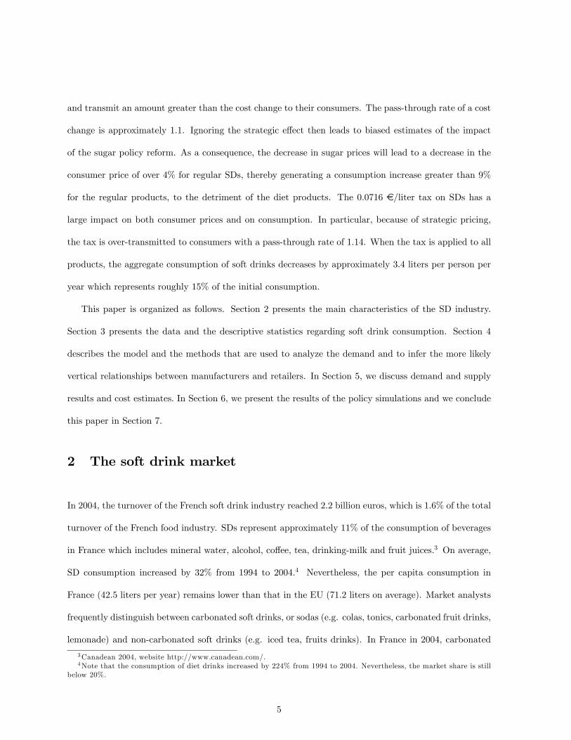
Table 2 shows the results of the demand model estimates by GMM that account for consumer hetero-

geneity regarding price sensitivity and the taste for observed product characteristics.12 First, note that

the over-identifying restriction test is not rejected which indicates that the instruments are valid. On

average, the price has a signi�cant and negative impact on utility. Given the value of the price standard

deviation, only 0.1% of the distribution of the price coe¢ cient is positive. The coe¢ cient of the dummy

that identi�es diet products is positive on average, which means that consumers like this characteristic.

The soda category is preferred to the fruit drink category, but consumers prefer fruit drinks to iced teas.

However, the standard deviations for both categories are large, which means that some consumers prefer

these categories and others do not.

Using the structural demand estimates, we are able to compute own and cross-price elasticities for each

11These indices are from the French National Institute for Statistics and Economic Studies.12This estimation was achieved using 500 draws for the parametric distribution that represents the unobserved consumer

characteristics and for the non-parametric distribution of the consumer demographics.

16

Table 2: Results of the random-coe¢ cients logit model.

Coe¢ cients (Std. error) Mean Standard Deviation

Price -7.04(0.41) 2.35 (0.43)Diet 0.52 (0.02) 0.26 (0.23)Soda category 1.90 (0.02) 2.96 (0.45)Ice tea category -0.71 (0.02) 2.89 (0.59)Coe¢ cients �j ; t not shownOveridentifying Restriction Test (df) 19.43 (15)

di¤erentiated products (Table 3).13 The own-price elasticities of demand for a brand vary between -2.37

and -4.90 with an average value of -4.06. The own price elatisticities of the NBs (average value of -4.6)

are larger, in absolute value, than the own price elasticities of the PLs (average value of approximately

-2.6). Other studies of the soft drink market report own price elasticities of a similar magnitude. For

example, Gasmi et al. (1992) estimate own price elasticities of -2 for Coca-Cola and Pepsi-Cola. For

the carbonated soft drink US market, Dhar et al. (2005) distinguished 4 brands and found own-price

elasticities between -2 and -4. Dube (2005) found elasticities ranging from -3 to -6 in the Denver area. It

is interesting to note that the substitutions primarily occur between products in the same categories.

To investigate whether consumers have a strong brand preference we compare the following alternatives

for a consumer. If the price of a brand increases, does a consumer switch to an other brand that is sold

by the same retailer, or does the customer prefer to switch between retailers in order to buy the same

brand? As shown by Steiner (1993), if the customer prefers to switch the brand, then the bargaining

power is in favor of the retailers; otherwise it is in favor of the manufacturers. We report in Table 3

the average of the cross-price elasticities of each brand computed within a retailer (switch of brand) and

within the same brand (switch of retailers). The results depend on the products. It is interesting to note

that for the leading products (product 3 is the leading regular product and product 4 is the leading diet

product) consumers prefer to switch their retailer to buy the prefered brand rather than switching to an

13The own price elasticity of a brand reported in the table 3 is the average of the own-price elasticity of this brand for thedi¤erent retailers. We also calculate two average cross-price elasticities for each brand. The �rst elasticity (within a retailer)is the average over all retailers of the average of cross-price elasticities of a brand with respect to any other brand sold at aretailer. The second elasticity (between the same brands) is the average of cross price elasticities of a brand with respect tothe same brand sold at any other retailer. All averages are weighted averages, and we use market shares as to weight them.

17

Table 3: Cross Price Elasticities between products

Brands Within a retailer Between same brands

B1 -4.20 (0.17) 0.003 (0.001) 0.001 (0.0004)B2 -4.36 ( 0.17) 0.004 (0.001) 0.002 (0.0006)B3 -4.60 (0.13) 0.039 (0.006) 0.182 (0.025)B4 -4.84 (0.12) 0.021 (0.005) 0.031 (0.009)B5 -4.78 (0.20) 0.005 (0.002) 0.012 (0.007)B6 -4.90 (0.20) 0.001 (0.001) 0.0005 (0.0004)B7 -4.31 (0.21) 0.004 (0.002) 0.003 (0.001)B8 -4.42 (0.19) 0.005 (0.002) 0.004 (0.002)B9 -4.35 (0.19) 0.003 (0.001) 0.001 (0.0007)B10 -4.08 (0.20) 0.003 (0.001) 0.002 (0.001)B11 -4.17 (0.14) 0.002 (0.001) 0.001 (0.0003)B12 -2.37 (0.13) 0.005 (0.001) 0.012 (0.003)B13 -2.76 (0.23) 0.002 (0.001) 0.012 (0.004)B14 -2.69 (0.10) 0.003 (0.001) 0.006 (0.001)

other brand sold by the same retailer. This preference is also the case for the PLs. PLs are signi�cantly

cheaper than NBs. If the price of a PL increases at a retailer, a consumer could prefer to buy another PL

(from another retailer) rather than buying a NB from the same retailer. This result suggests that some

manufacturers have market power in this market ,which is consistent with our assumption regarding the

game that gives all bargaining power to the manufacturers.

5.2 Preferred model, price-cost margins and cost estimates

Using the demand estimates, we are able to compute the price cost margins for each supply model.

On the basis of the Rivers and Vuong tests (see the results in Table 10 in the appendix) the best

supply model is the model where the manufacturers and the retailers use two-part tari¤ contracts with

resale price maintenance14 , the wholesale margin is equal to zero, and where the private labels have no

strategic role in the manufacturer-retailer relationships. This result is consistent with the idea that in

this industry, brands are strong and thus provide market power to the upstream producers. According

to these results, the price cost margins are 45.25% of the consumer price, on average. The margins are

14Resale price maintenance (RPM) is prohibited by the competition authorities. However, in France, speci�c laws for theretail industry have led to a situation where it is, in practice, possible to implement RPM (Biscourp et al., 2008).

18

relatively heterogeneous across brands (see Table 8 in the appendix). The average price-cost margins

for the PLs (38.65%) are signi�cantly lower than those for the NBs (47.43%). The price-cost margins

do not di¤er across retailers except for retailer 8 which has lower margins because it only sells PLs, and

retailer 9, which has a higher average margin because it sells brands 1 and 2 with high margins as well as

PLs. The estimated marginal cost calculated from the best supply model is 0.45e/liter on average. The

average marginal cost of the PLs (0.30e/liter) is lower than that of the NBs (0.50e/liter).

6 Simulations

We de�ne three policy scenarios. Scenario 1 simulates the impact of a signi�cant decrease in the EU

sugar price. As explained above, the reference price of sugar, which roughly acts as a �oor price, was

reduced by 36% over a 4-year period starting in 2006.15 The actual decrease from 2006 to 2010 was

approximately 25% from 636 e/t in 2006 to 477 e/t in April 2010.16 Scenarios 2 and 3 simulate the

excise tax of e0.0716 per liter for soft drinks voted on December 28, 2011 by the French representatives.

Because there was a debate about the scope of the tax, we simulate both the initial proposal, which taxes

only regular, or sweetened, products (scenario 2), and the selected proposal, which taxes both regular

and diet products (scenario 3).

6.1 The impact of the sugar policy reform

Consistent with the anticipated impact of EU sugar policy reform, we simulate a 36% decrease in the sugar

price.17 Using the estimated marginal cost speci�cation for the best supply model, we �nd a decrease of

2.61 e cents/liter (or 8.34%) in the total marginal cost of regular soft drinks, which is very close to the

estimate obtained with an accounting calculation (approximately 2 e cents/liter). Cost decreases vary

15The reference price for white sugar was 631.9e/t from July 1, 2006 to September 30, 2008. It was 541.5e/t fromOctober 1, 2008 to September 30, 2009 and 404.4e/t after October 1, 2009.16http://ec.europa.eu/agriculture/minco/manco/cmo/index.htm17The impacts on price and consumption are roughly linear in terms of the percentage change of sugar price. The impact

of a 25% decrease in sugar price (as observed from 2006 to 2010) will then be roughly equal to 25/36 of the reported results.

19

across brands (Table 4) because the sugar content and the marginal cost di¤er across brands. Thus, the

marginal cost of a PL is lower than the marginal cost of a NB, which partly explains the larger percent

decrease in the marginal cost of the PLs.

Table 4: Impact of a decrease in the sugar priceChange in cost Change in price Pass-through Change in MS

in % in % 4p=4c in %Mean (std) Mean (std) Mean (std) Mean (std)

Brand 1 NB R -12.84 (1.60) -4.87 (0.19) 1.09 (0.03) 11.79 (1.27)Brand 2 NB D � 0.85 (0.11) - -12.12 (0.90)Brand 3 NB R -7.14 (0.39) -3.57 (0.10) 1.09 (0.03) 9.18 (1.06)Brand 4 NB D � 0.75 (0.08) - -11.48 (0.81)Brand 5 NB R -3.35 (0.21) -2.05 (0.13) 1.07 (0.03) 3.63 (0.76)Brand 6 NB D � 0.57 (0.06) - -8.94 (0.73)Brand 7 NB R -4.13 (0.22) -2.82 (0.16) 1.16 (0.03) 7.74 (0.70)Brand 8 NB R -4.26 (0.15) -3.14 (0.11) 1.23 (0.04) 9.77 (0.55)Brand 9 NB D � 0.66 (0.06) - -7.47 (0.86)Brand 10 NB R -5.09 (0.37) -3.28 (0.19) 1.13 (0.03) 9.19 (0.63)Brand 11 NB R -5.31 (0.28) -3.57 (0.13) 1.17 (0.03) 10.82 (0.59)Brand 12 PL R -18.22 (1.79) -8.96 (0.42) 1.03 (0.01) 12.16 (0.89)Brand 13 PL R -9.58 (1.34) -5.25 (0.26) 1.06 (0.02) 7.60 (0.72)Brand 14 PL R -9.65 (0.49) -6.13 (0.20) 1.11 (0.01) 12.86 (0.43)

On average, in response to the price cut, consumer prices decrease by 4.48% for the regular products.

Note that the percent price decrease for the PLs is larger than that for the NBs because the PLs are

cheaper than the NBs. For regular products, the pass-through, which is measured by the ratio of the

di¤erence in retail prices to the di¤erence in marginal costs, has an average value of 1.10. Therefore, if

the marginal cost decreases by 1 e cent/liter the retail price decreases by an average of 1.10 e cents/liter.

The industry thus overshifts the cost decrease. This result is consistent with the supply model. Indeed,

the contract that best �ts the data (two part-tari¤ contracts with resale price maintenance and zero

manufacturer gross margins; in the following, we denote this contract as the �selected�contract) allows

the industry to behave non-competitively. This contract maximizes the total pro�t of the entire chain

in the absence of private labels (Bonnet and Dubois, 2010). Moreover, Rey and Tirole (2007) showed

that a monopoly producer facing several retailers can use this type of contract to implement a monopoly

situation. Carbonnier (2006) showed that under imperfect competition the cost pass-through could be

less than or greater than 100% depending on the curvature of the demand. This result is also consistent

20

with the reduced form analysis of Campa and Goldberg (2006) who found that the pass-through rates

in the food industry in France are larger than one (1.41). Besley and Rosen (1999) also found, in the

case of the US, that the SD industry overshifts tax changes. According to them, this overshifting is a

consequence of the imperfect competition in this industry.

The pass-through varies by brand from 1.03 to 1.23; therefore it is important to consider the strategic

behavior of the producers of di¤erentiated products. It should be acknowledged that the model integrates

the brand portfolio of the manufacturers. Thus manufacturers choose a pricing policy for the entire set

of products, thereby internalizing the substitution among their own set of products. The price of diet

products does not change signi�cantly; it increases by less than 1%. As a result of these strategic reactions,

the aggregate market share of the regular products increases by 9.56% by replacing diet products, whose

market share decreases by 10.85%, and the outside option, whose market share decreases by 5.6%.18

6.2 The impact of a tax on soft drinks

As mentioned above, the appropriate scope of SDs taxation was debated by the French parliament. For

some representatives the proposed tax (7.16 e cents/liter) should apply only to the sweetened (regular)

SDs. In this case, the tax would increase public revenues (the main objective) but it could also reduce the

consumption of sweetened SDs. The tax was presented as an �obesity tax�because a high consumption

of sweetened SDs is frequently associated with obesity; this idea is opposed by the representatives of the

French Food Industry (ANIA) who are strongly against the idea of a health policy based on taxation.

In the end, the scope of the tax was enlarged to include all SDs, regardless of whether they incorporate

added sugar, and is no longer presented as an obesity tax. We simulate both options and evaluate the

changes created by the tax (Table 5).

The proposed tax is approximately 10% of the price of the SDs. When the tax only applies to regular

products, the price of the regular products increases by over 13%, on average. Strategic pricing increases

18Note that the price of the outside option is assumed to be unchanged, which is a limit in the analysis. However, asigni�cant part of the goods in the outside option will not be a¤ected by the decrease in the sugar price as those goods donot contain any added sugar.

21

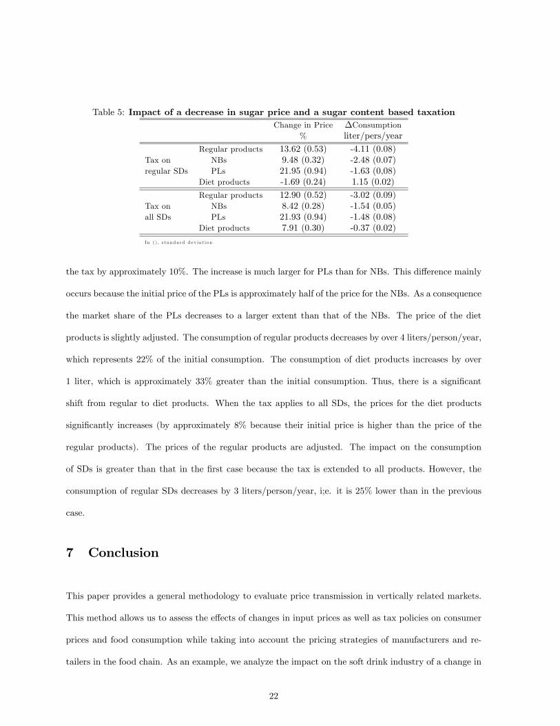
Table 5: Impact of a decrease in sugar price and a sugar content based taxationChange in Price �Consumption

% liter/pers/year

Regular products 13.62 (0.53) -4.11 (0.08)Tax on NBs 9.48 (0.32) -2.48 (0.07)regular SDs PLs 21.95 (0.94) -1.63 (0,08)

Diet products -1.69 (0.24) 1.15 (0.02)

Regular products 12.90 (0.52) -3.02 (0.09)Tax on NBs 8.42 (0.28) -1.54 (0.05)all SDs PLs 21.93 (0.94) -1.48 (0.08)

Diet products 7.91 (0.30) -0.37 (0.02)

In ( ) , s t a n d a rd d e v ia t io n

the tax by approximately 10%. The increase is much larger for PLs than for NBs. This di¤erence mainly

occurs because the initial price of the PLs is approximately half of the price for the NBs. As a consequence

the market share of the PLs decreases to a larger extent than that of the NBs. The price of the diet

products is slightly adjusted. The consumption of regular products decreases by over 4 liters/person/year,

which represents 22% of the initial consumption. The consumption of diet products increases by over

1 liter, which is approximately 33% greater than the initial consumption. Thus, there is a signi�cant

shift from regular to diet products. When the tax applies to all SDs, the prices for the diet products

signi�cantly increases (by approximately 8% because their initial price is higher than the price of the

regular products). The prices of the regular products are adjusted. The impact on the consumption

of SDs is greater than that in the �rst case because the tax is extended to all products. However, the

consumption of regular SDs decreases by 3 liters/person/year, i;e. it is 25% lower than in the previous

case.

7 Conclusion

This paper provides a general methodology to evaluate price transmission in vertically related markets.

This method allows us to assess the e¤ects of changes in input prices as well as tax policies on consumer

prices and food consumption while taking into account the pricing strategies of manufacturers and re-

tailers in the food chain. As an example, we analyze the impact on the soft drink industry of a change in

22

the sugar price or the introduction of an excise tax. Using the recent development of empirical industrial

organization, we have estimated a very �exible demand model, a random coe¢ cients logit model, and

several models for the vertical relationships within the industry. We have shown that the most likely sup-

ply model is the model where the manufacturers and the retailers use two-part tari¤ contracts with resale

price maintenance and where the private labels play no role in the manufacturer/retailer relationships.

In this case, the manufacturers have a signi�cant market power which is a consequence of the strength

of their brands. This result is consistent with anecdotal evidence regarding this speci�c industry, such as

the advertising investments of �rms to build a strong reputation. Using this model, we have simulated

the impact on prices for alternative policy scenarios that take into account the strategic choices of agents.

We have shown that, on average, the pass-through is greater than 1; the industry would then transmit

more than the change in cost (when analyzing a change in input cost) or more than the excise tax to the

consumers. Our results then suggest that the assumption of passive pricing by the industry would result

in an under-estimation of the change in retail prices and thus in consumption.

According to these results, any analysis of the impact of food price policies requires that the strategic

pricing of the �rms be addressed. One di¢ culty is that we cannot easily extrapolate our results to other

industries. Neither the type of contracts used by a speci�c industry nor the qualitative results (e.g., the

overshift of cost changes) can be generalized. First, the structure of the upstream industry plays a role

in the choice of contracts between the processors and the retailers. In the speci�c case of food markets,

the structure of the upstream industry varies signi�cantly from a low level of concentration (e.g., the

meat industry or the wine industry) to a high level of concentration (e.g., the processed cheese industry

or the water industry). Second, the strategic response depends on the curvature of the demand, which is

also market-speci�c. As a consequence, the empirical analysis of price transmission in a given industry

requires that the vertical relationships of this speci�c industry be evaluated �rst.

Our analysis of the impact of the tax is related to the market conditions in 2003-2005. To extrapolate

the results to the present situation, at least two elements must be integrated. First, the size of the market

has certainly changed between 2005 and 2011. Second, SD prices have changed, and thus the shock created

23

by the tax as a percentage is di¤erent.

One limitation of our analysis is the implicit assumption that the price of the outside option does

not changed, regardless of the policy. With this assumption the products included in the outside option

are supposed not to be directly a¤ected by the policy scenarios. In our case, many goods in the outside

option will not be a¤ected by a decrease in the sugar price because these goods do not contain any added

sugar and they will also not be a¤ected by the proposed excise tax. However, this assumption also means

that the producers and the retailers of the outside good do not strategically react to any changes in the

prices of the market under scrutinity. This option is acceptable if the market of the outside option is

su¢ ciently competitive.

References

Anderson, S. P., de Palma, A., Kreider, B., 2001. Tax incidence in di¤erentiated product oligopoly.

Journal of Public Economics 81 (2), 173 �192.

URL http://www.sciencedirect.com/science/article/pii/S0047272700000797

Bergès-Sennou, F., Bontems, P., Réquillart, V., 2004. Economics of private labels: A survey of literature.

Journal of Agricultural and Food Industrial Organization 2(3).

Berry, S., Levinsohn, J., Pakes, A., 1995. Automobile prices in market equilibrium. Econometrica 63,

841�890.

Berto Villas-Boas, S., 2007. Vertical relationships between manufacturers and retailers: Inference with

limited data. Review of Economic Studies 74, 625�652.

Bettendorf, L., Verboven, F., 2000. Incomplete transmission of co¤ee bean prices: evidence from the

netherlands. European Review of Agricultural Economics 27(1), 1�16.

Biscourp, P., Boutin, X., Vergé, T., 2008. 2008. the e¤ects of retail regulation on prices : evidence from

french data. INSEE-DESE Working Paper G2008/02, Paris France.

24

Bonnet, C., Dubois, P., 2010. Inference on vertical contracts between manufacturers and retailers allowing

for non linear pricing and resale price maintenance. Rand Journal of Economics 41(1), 139�164.

Bonnet, C., Dubois, P., Villas-Boas, S., 2009. Empirical evidence on the role of nonlinear wholesale pricing

and vertical restraints on cost pass-through. UC Berkeley, Department of Agricultural and Resource

Economics, UCB.

Bukeviciute, L., Dierx, A., Ilzkovit, F., 2009. The functioning of the food supply chain and its e¤ect on

food prices in the european union. Tech. rep., European Economy, Occasional papers 47.

Campa, J. M., Goldberg, L. S., 2006. Pass through of exchange rates to consumption prices: What has

changed and why? In International Financial Issues in the Paci�c Rim: Global Imbalances, Financial

Liberalization and Exchange Rate Policy. NBER and University of Chicago Press.

Carbonnier, C., 2006. Fiscalité optimale et incidences �scales. analyses théoriques et estimations sur

réformes françaises de la taxe sur la valeur ajoutée et de la taxe professionnelle, 1987-2004. Ph.D.

thesis, Ecole des Hautes Etudes en Sciences Sociales, Paris-jourdan Sciences Economiques.

Dhar, T., Chavas, J., Cotterill, R., Gould, B., 2005. An economeric analysis of brand-level strategic

pricing between cocal-cola company and pepsico. Journal of Economics and Management Strategy

14(4), 905�931.

Dube, J.-P., 2005. Product di¤erentiation and mergers in the carbonated soft drink industry. Journal of

Economics and Management Strategy 14(4), 879�904.

Gasmi, F., La¤ont, J., Vuong, Q., 1992. Econometric analysis of collusive behavior in a soft-drink market.

Journal of Economics & Management Strategy 12(1), 277�311.

Hellerstein, R., 2008. Who bears the cost of a change in the exchange rate? pass-through accounting for

the case of beer. Journal of International Economics 76 (1), 14 �32.

URL http://www.sciencedirect.com/science/article/pii/S0022199608000299

25

Kim, D., Cotterill, R. W., 2008. Cost pass-through in di¤erentiated product market: the case of u.s.

processed cheese. The Journal of Industrial Economics LV (1), 32�48.

McFadden, D., Train, K., 2000. Mixed mnl models for discrete response. Journal of applied Econometrics

15(5), 447�470.

Nakamura, E., Zerom, D., 2010. Accounting for incomplete pass-through. Review of Economic Studies,

forthcoming.

Nevo, A., 2000. Mergers with di¤erentiated products: the case of the ready-to-eat cereal industry. RAND

Journal of Economics 31, 395�421.

Nevo, A., 2001. Measuring market power in the ready-to-eat cereal industry. Econometrica 69, 307�342.

OECD, 2011. OECD-FAO Agricultural Outlook 2011-2020. OECD.

Rey, P., Tirole, J., 2007. A primer on foreclosure. Handbook of Industrial Organization Elsevier.

Rey, P., Vergé, T., 2004. Resale price maintenance and horizontal cartel". CMPO Working Papers series

No. 02/047, University of Southampton.

Rivers, D., Vuong, Q., 2002. Model selection tests for nonlinear dynamic models. The Econometrics

Journal 5(1), 1�39.

Steiner, R., 1993. The inverse association between the margins of manufacturers and retailers. Review of

Industrial Organization 8, 717�740.

Sudhir, K., 2001. Structural analysis of manufacturer pricing in the presence of a strategic retailer.

Marketing Science 20(3), 244�264.

Vavra, P., Goodwin, B. K., 2005. Analysis of price transmission along the food chain. OECD Food,

Agriculture and Fisheries Working Papers, No. 3, OECD Publishing.

26

8 Appendices

8.1 Descriptive statistics on data

Table 6: Descriptive Statistics for Prices and Market Shares by Brands.

Prices (in euros per liter) Market SharesMean (std) Mean in % (std)

Brand 1 0.67 (0.03) 2.52 (0.43)Brand 2 0.70 (0.03) 3.13 (0.64)Brand 3 0.87 (0.02) 33.06 (2.72)Brand 4 0.90 (0.02) 13.08 (0.96)Brand 5 1.03 (0.04) 3.85 (1.21)Brand 6 1.03 (0.05) 0.71 (0.22)Brand 7 1.00 (0.04) 3.80 (0.52)Brand 8 1.11 (0.03) 3.74 (0.81)Brand 9 1.00 (0.05) 2.41 (0.60)Brand 10 0.86 (0.05) 4.40 (0.69)Brand 11 0.90 (0.02) 2.50 (0.36)Brand 12 0.33 (0.01) 9.04 (0.66)Brand 13 0.43 (0.03) 5.80 (1.14)Brand 14 0.44 (0.01) 11.90 (1.13)

27

Table 7: Descriptive Statistics for Prices and Market Shares by Retailers.

Prices (in euros per liter) Market SharesMean (std) Mean in % (std)

Retailer 1 0.86 (0.03) 13.32 (0.95)Retailer 2 0.85 (0.03) 16.54 (1.12)Retailer 3 0.87 (0.03) 8.14 (0.58)Retailer 4 0.84 (0.03) 12.42 (0.97)Retailer 5 0.77 (0.02) 20.49 (1.13)Retailer 6 0.80 (0.04) 8.85 (0.80)Retailer 7 0.89 (0.03) 5.21 (0.37)Retailer 8 0.48 (0.02) 1.96 (0.30)Retailer 9 0.35 (0.1) 13.02 (1.30)

8.2 Detailed proof of the manufacturers pro�t expression

Manufacturers can adjust franchise fees such that all constraints are binding. So the participation con-

straint for the retailer r becomes:

Xj2Sr

[M(pj � wj � cj)sj(p)� Fj ] =Pj2eSrM(eprj � wj � cj)sj(epr)X

j2Sr

Fj =Xj2Sr

M(pj � wj � cj)sj(p)�Pj2eSrM(eprj � wj � cj)sj(epr)X

j2Gf

Fj +Xj =2Gf

Fj =RPr=1

Xj2Sr

Fj =JXj=1

M(pj � wj � cj)sj(p)�RPr=1

Pj2eSrM(eprj � wj � cj)sj(epr)

Xj2Gf

Fj =JXj=1

M(pj � wj � cj)sj(p)�RPr=1

Pj2eSrM(eprj � wj � cj)sj(epr)�

Xj =2Gf

Fj

Therefore, we can re-write the pro�t of the manufacturer as:

�f =Xj2Gf

M(wj � �j)sj(p) +JXj=1

M(pj � wj � cj)sj(p)�RPr=1

Pj2eSrM(eprj � wj � cj)sj(epr)�

Xj =2Gf

Fj (7)

28

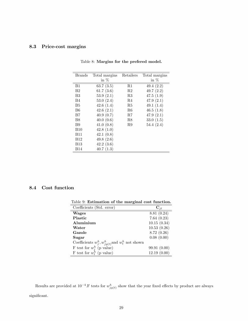
8.3 Price-cost margins

Table 8: Margins for the prefered model.

Brands Total margins Retailers Total marginsin % in %

B1 63.7 (3.5) R1 49.4 (2.2)B2 61.7 (3.6) R2 49.7 (2.2)B3 53.9 (2.1) R3 47.5 (1.9)B4 53.0 (2.4) R4 47.9 (2.1)B5 42.6 (1.4) R5 49.1 (1.4)B6 42.6 (2.1) R6 46.5 (1.8)B7 40.9 (0.7) R7 47.9 (2.1)B8 40.0 (0.6) R8 33.0 (1.5)B9 41.0 (0.8) R9 54.4 (2.4)B10 42.8 (1.0)B11 42.1 (0.8)B12 49.8 (2.6)B13 42.2 (3.6)B14 40.7 (1.3)

8.4 Cost function

Table 9: Estimation of the marginal cost function.Coe¢ cients (Std. error) Cjt

Wages 8.81 (0.24)Plastic 7.64 (0.23)Aluminium 10.15 (0.34)Water 10.53 (0.26)Gazole 8.72 (0.26)Sugar 0.08 (0.00)Coe¢ cients whj ; w

hjy(t)and w

ht not shown

F test for whj (p value) 99.91 (0.00)F test for wht (p value) 12.19 (0.00)

Results are provided at 10�4:F tests for whjy(t) show that the year �xed e¤ects by product are always

signi�cant.

29

8.5 Non-nested tests

Table 10: Non-nested Rivers and Vuong tests.Rivers and Vuong Test Statistic Tn� H2H1 2 3 4 5 6 71 -4.64 -3.92 2.23 -4.15 -2.62 2.462 11.90 2.27 4.75 7.07 2.513 2.26 -2.20 4.18 2.504 -2.27 -2.25 0.685 8.19 2.506 2.49

Model 1 is double marginalisation, Model 2 is two part tari¤s with resale price maintenance and

w = �, Model 3 is two part tari¤s with resale price maintenance and p � w � c = 0, Model 4 is two

part tari¤s without resale price maintenance, Model 5 is two part tari¤s with resale price maintenance

and w = � and private labels buyer power, Model 6 is two part tari¤s with resale price maintenance,

p�w�c = 0 and private labels buyer power, Model 7 is two part tari¤s without resale price maintenance

and private labels buyer power

30