SUITABLE CONTROL LAWS TO PATH TRACKING IN OMNIDIRECTIONAL

WHEELED MOBILE ROBOTS SUPPORTED BY THE MEASURING OF THE

ROLLING PERFORMANCE

C. A. Pena Fernandez∗ J. J. F. Cerqueira∗ A. M. N. Lima†

∗Laboratorio de Robotica - Programa de Pos-graduacao em Engenharia Eletrica

da Escola Politecnica da Universidade Federal da Bahia

Rua Aristides Novis, 02, Federacao, 40210-630, Salvador, Bahia, Brasil

Telefone:+55-71-3203-9760.

†Departamento de Engenharia Eletrica do Centro de Engenharia Eletrica e Informatica da

Universidade Federal de Campina Grande

Rua Aprigio Veloso, 882, Universitario, 58429-970, Campina Grande, Paraıba, Brasil

Telefone:+55-83-2101-1000.

Email: cesar.pena@ufba.br,jes@ufba.br,amnlima@dee.ufcg.edu.br

Abstract— This work proposes a method in order to choose suitable control laws supported in the measuringof the rolling performance in omnidirectional wheeled mobile robots when the holonomic kinematic constraintsare not fully satisfied. One important reason that causes such dissatisfaction is the slip presents at wheels and,consequently, the inappropriate conditions for the rolling. The appropriate rolling conditions for omnidirectionalwheeled mobile robots are defined by zero slip rate (i.e., s = 0) and nonzero slip (i.e., s 6= 0) (Fernandezet al., 2012). By using the singular perturbation theory the slip can be included into overall dynamic of themobile robot and it is possible to project control actions that mitigate the slip. Here, an expression to measuringthe slip rate is derived in order to accessing the rolling performance in the mobile robot. Supporting us in suchexpression is possible to choose the suitable control law that ensures fully the appropriate rolling conditions. Thismethodology was applied in an experimental platform called AxeBot that is being constructed in the RoboticsLaboratory at University Federal of Bahia and that uses odometry for the self-localization.

Keywords— Omnidirectional mobile base, slip, corrective control actions, rolling performance, singular per-turbation theory.

Resumo— Este trabalho propoe um metodo para escolher leis controle apropriadas apoiado na medida dodesempenho do rolamento em robos moveis omnidirecionais quando as restricoes cinematicas holonomicas naosao completamente satisfeitas. Uma das razoes mais importantes que causa tal insatisfacao e o escorregamentopresente nas rodas e, consequentemente, as condicoes inapropriadas de rolamento. As condicoes apropriadas derolamento para robos moveis omnidirecionais sao definidas por uma variacao de escorregamento nula e por umvalor de escorregamento diferente de zero (Fernandez et al., 2012). Pelo uso da teoria de perturbacoes singulareso escorregamento pode ser incluıdo na dinamica geral do robo e e possıvel projetar leis de controle que atenuamo escorregamento. Aqui, uma expressao para medir a variacao do escorregamento e derivada a fim de acessar odesempenho do rolamento no robo movel. Apoiando-nos em tal expressao e possıvel escolher a lei de controleadequada que garante a satisfacao das condicoes de rolamento apropriada. Esta metodologia foi aplicada em umaplataforma experimental chamada Axebot que esta sendo construıda no Laboratorio de Robotica da UniversidadeFederal da Bahia e que usa odometria para sua auto-localizacao.

Palavras-chave— Base movel omnidirecional, escorregamento, acoes de controle corretivas, desempenho dorolamento, teoria de pertubacoes singulares.

1 Introduction

In this paper we have formulated a methodology tochoose the suitable control laws such that the ap-propriate rolling conditions are satisfied (Fernandezet al., 2012). We apply our methodology to validatea control law with corrective actions for the trajec-tory tracking problems in the AxeBot, an omnidirec-tional wheeled mobile robot (OWMR) that is beingconstructed in the Robotics Laboratory at Univer-sity Federal of Bahia for research and developmentof the trajectory control (see Fig. 1(a)). To imple-ment this methodology is considered that omnidirec-tional motion of the Axebot do not satisfy its holo-nomic kinematic constraints as a consequence of theslippage. A condition usually considered for trajec-tory tracking problems in mobile robots is the idealrolling assumption, i.e., the wheels of a mobile robotare assumed to roll without slipping. But disregar-

ding the slip of wheels in the dynamic model leadsus to path tracking problems (Fernandez and Cer-queira, 2009a; Motte and Campion, 2000). When therobot is either accelerating, or decelerating, or cor-nering at a high speed the wheel slip becomes an is-sue and the ideal rolling assumption is not satisfied(Fernandez and Cerqueira, 2009b; Fernandez and Cer-queira, 2009a). If the slip is not taken into account,a designed task may not be completed and a stablesystem may even become unstable. One of the mostimportant reasons for this problem is when the trajec-tory tracking is made by using odometry to calculatingthe cartesian position. This methodology has been wi-dely used, largely because of its easy implementation,but its disadvantage is the unlimited accumulation oferrors in the control scheme due to slip in the wheels,among other intrinsic properties of the surface motion(Song and Wang, 2009; Ivankjo et al., 2004; Bahariet al., 2008; Trojnacki, 2013). In the AxeBot, the self-

(a)

L

x1

x2

θ

φ1

φ2

φ3

p

{G}

{R}

(b)

Figura 1: Photograph of (a) the experimental platform AxeBotand (b) Kinematic structure of the omnidirectional wheeledmobile robot with global frame {G} and local frame {R}.

localization is made with Odometry, thus this platformoffers a convenient problem situation which will allowto verify if the control law applied will guarantee agood rolling performance.

With the problem of the slipping we have consi-dered that the AxeBot can be modeled by a singularlyperturbed model. Assuming that there exists an inva-riant manifold for the slip, corrective control actionsare projected by using the singular perturbation the-ory such that slip in the wheels is mitigated (Motteand Campion, 2000; D’andrea-novel et al., 1995). Wepropose to use an expression to caracterize the sliprate related to trajectory tracking problems as tool tomeasuring the rolling performance. By using the expe-rimental platform AxeBot such tool is used as supportto choose the suitable control law.

This paper is organized as follows: In Section2, the key aspects regarding OWMRs and the inclu-sion of slip nonlinearity into the proposal of the sin-gularly perturbed model are discussed. In Section 3is shown the proposal to measuring the rolling per-formance. In Section 4 an invariant manifold for slipis defined and computed such that corrective controlactions can be projected to minimize the errors intothe control scheme due to the existence of slip. InSection 5 the proposed approach is used for accessingthe achievable closed-loop performance with the cor-rective control actions projected and it is discussedthe observations obtained. Finally, conclusions andclosing remarks are shown in Section 6.

2 Mathematical Dynamic Model

The configuration of AxeBot mobile robot can be fullydescribed by the vector q ∈ R

6 of generalized coordi-nates defined by

q = [x1 x2 θ φ1 φ2 φ3]T

where {x1, x2, θ} is the set of coordinates associatedwith the cartesian position of the local frame {R} intothe global frame {G} and guidance of mobile base,and {φ1, φ2, φ3} is the set associated with the angularposition of each wheel [which can not be controlledindependently] (see Fig. 1(b)).

The kinematic constraints can be expressed as thePfaffian constraint (Motte and Campion, 2000)

AT (q)q = 0 (1)

where A(q) is the matrix with the holonomic kinema-tic constraints defined by

A(q) =

− sinα sin θ sinβ− cosα − cos θ − cos β

b b br 0 00 r 00 0 r

,

[

A1(θ)

A2(θ)

]

,

where α = θ − 2π3, β = θ + 2π

3, b is the displacement

from each of driving wheels to the axis of symmetryof mobile base, r is the radius of each wheel.

Provided that the ideal kinematic constraints arenot satisfied [i.e., AT (q)q 6= 0], then the generalizedvelocity vector q may be written as

q = S(q)v + A(q)εs, (2)

such that

AT (θ)S(q) = 0, (3)

where

S(q) =

cos θ sin θ 0− sin θ cos θ 0

0 0 1−√

3/2r 1/2r b/r0 −1/r b/r

√3/2r 1/2r b/r

,

[

S1(θ)

S2(θ)

]

,

is the Jacobian, v = [v1 v2 v3]T is the vector that con-

tains the velocities at the wheels and s = [s1 s2 s3]T

contains the slip at each wheel. This last one canbe considered as instrumental vector in sense of acces-sing the violations of the ideal kinematic constraints inOWMRs. It is important to mention that when thereis slip, the vector q becomes an apparent quantity q.

As usual, the dynamic model for such mobile baseis given by

Mq = Λ +Buε + A(θ)λ (4)

where M = diag (M M Ic Iw Iw Iw), Λ = 06×1, B =[03×3

I3×3

]

are the inertia matrix, the centripetal and co-

riolis torques [equal to zero because is assumed thatthe geometrical center coincides with the mass center]and a full rank matrix, respectively. The parameterM is the mass of mobile base, Ic is the moment ofinertia of mobile base about a vertical axis throughthe intersection of the axis of symmetry with the dri-ving wheel axis and Iw is the moment of inertia ofeach driving wheel about the wheel axis. The vectoruε represents of the input forces or torques providedby the actuators and λ ∈ R

3 represents of Lagrangemultipliers (Balakrishna and Ghosal, 1995).

2.1 Singularly perturbed model

The singularly perturbed formulation to the dynamicof AxeBot is defined by the following state-space des-cription:

x = B0(q)v + [εB1(q) + B2(q)] s+ B3(q)uε (5)

εs = C0(q)v + [εC1(q) + C2(q)] s+ C3(q)uε (6)

y = P0(q) (7)

where x =[qT vT

]Tcan be used to denote the “slow”

variables and s beyond its instrumental meaning canbe used to denote the “fast” variables; ε is a smallpositive parameter, uε = [uε,1 uε,2 uε,3]

T are the ma-nipulated inputs associated with the torques at themotors and y = [y1 y2]

T are the cartesian coordinates

of a point p located at a distance L of the symmetryaxle of the robot, i.e.:

y = P0(q) ,[

x1−L sin θx2+L cos θ

]

= P0(θ). (8)

The above matrices Bi(q), Ci(q), for i = 0, 1, 2, 3,are successively:

B0(q) =

[S(θ)

a1 a2 a3a4 a5 a6a7 a8 a9

]

, B1(q) =

[A(θ)

a10 a11 a12a13 a14 a15a16 a17 a18

]

,

B2(q) =

[06×3

a28 a29 a30a31 a32 a33a34 a35 a36

]

, B3(q) =

[06×3

a19 a20 a21a22 a23 a24a25 a26 a27

]

,

C0(q) =[ a37 a38 a39a40 a41 a42a43 a44 a45

]

, C1(q) =[ a46 a47 a48a49 a50 a51a52 a53 a54

]

,

C2(q) =[ a64 a65 a66a67 a68 a69a70 a71 a72

]

, C3(q) =[ a55 a56 a57a58 a59 a60a61 a62 a63

]

,

being ai, for i = 1, . . . , 72, known values and definedby

ai , ai(vη, δ,Do, Go),

where the parameter vη is the velocity of the wheelcenter and δ is a “small” positive constant to avoid thenumerical problem for small values of vη [i.e., for smallvalues of vη , it is replaced by vη + δ]. The parametersDo and Go are normalized values defined by

Do = εD and Go = εG,

where D and G are the stiffness coefficients for thetransversal and longitudinal movements of each wheel,respectively.

Assumption 1 The longitudinal and transversalstiffness coefficients (G and D, respectively) are thesame for the three wheels and

ε = inf{1/G, 1/D}.

Assumption 2 The velocities of the three drivingwheels at their center are taken to be identical, andmore precisely, equal to their average:

vη =(

x21 + x2

2 + θ2)1/2

. (9)

2.2 Interaction forces at wheels

Since OWMRs have only constraints associated withrolling conditions, in this work, the contact forces arerepresented in terms of the relationship between thelongitudinal slip ratio of each wheel, si, and its res-pective friction coefficient µi.

Assumption 3 The friction coefficients µi (for i =1, 2, 3) are taken to be identical due to symmetric massdistribution, and more precisely, equal to

µi = Mr3

Mgvi , zovi

where Mr is the mass of each driving wheel and g isthe gravity.

Burckhardt’s model, for instance, can be used todescribe the nonlinear characteristics of the contactforces (Fernandez et al., 2012; Canudas de Wit et al.,2003). For our purpose, this map is defined by

µi = c1(1− e−c2si

)− c3si

∣∣∣c1=1; c2=2; c3=0.1

, (10)

for i = 1, 2, 3. Where the parameters c1, c2, c3 aresetting for humidity conditions, as shown in (Canudasde Wit et al., 2003). In this mapping si ∈ [−1,+1]and µi ∈ R.

3 Rolling dynamic analysis

The appropriate rolling conditions in the OWMR mo-tion can be defined by

{

s 6= 0

s = 0.(11)

The condition s 6= 0 means that the mechanicaltorques are not large enough to ensure that the wheel-surface contact point stay stationary. It is importantto point out that such condition is an inherent andproper feature of OWMRs motion (Fernandez et al.,2012; Balakrishna and Ghosal, 1995).

3.1 Proposal to measuring the rolling performance

The rolling dynamics are analyzed according to thesatisfaction of the appropriate rolling condition defi-ned in (11). In following will be presented an analysisassociated with the longitudinal rolling that will allowto define a criteria to choose a suitable control law.

The apparent linear velocities of wheels can beassociated with the apparent linear velocity of the mo-bile base by using (2) and via the pseudo-inverse ma-trix S+(q)

v = S+(q) (q −A(q)εs)

, S+(θ)[

x1 − A1(θ)εs . . . φ3 − A6(θ)εs]T

, S+(θ)[

˙x1˙x2

˙θ . . .

˙φ3

]T

︸ ︷︷ ︸˙q

where Ai(θ) represent the i-th row of A(θ).By using the Assumption 3 we have

µ = zov,

and by defining the components of S+(θ) as πij(θ),the i-th friction coefficient can be expressed by

µi = zovi,

µi = zod

dt

(

πi1˙x1 + . . .+ πi3

˙θ + . . .+ πi6

˙φ3

)

,

µi = zo

(∂πi1

∂θ

˙θ ˙x1 + πi1

¨x1

+∂πi2

∂θ

˙θ ˙x2 + πi2

¨x2 +∂πi3

∂θ

˙θ2 + πi3

¨θ

+∂πi4

∂θ

˙θ˙φ1 + πi4

¨φ1 +

∂πi5

∂θ

˙θ˙φ2 + πi5

¨φ2

+∂πi6

∂θ

˙θ˙φ3 + πi6

¨φ3

)

,

since S+(θ) depends only on θ. Taking the time deri-vative of µi yields

µi =zo

(d

dt

(∂πi1

∂θ

˙θ

)

˙x1 + 4∂πi1

∂θ

˙θ ¨x1

+d

dt

(∂πi2

∂θ

˙θ

)

˙x2 + 4∂πi2

∂θ

˙θ ¨x2

+d

dt

(∂πi3

∂θ

˙θ

)

˙θ + 5

∂πi3

∂θ

˙θ¨θ

+d

dt

(∂πi4

∂θ

˙θ

)

˙φ1 + 4

∂πi4

∂θ

˙θ¨φ1

+d

dt

(∂πi5

∂θ

˙θ

)

˙φ2 + 4

∂πi5

∂θ

˙θ¨φ2

+d

dt

(∂πi6

∂θ

˙θ

)

˙φ3 + 4

∂πi6

∂θ

˙θ¨φ3

+ πi1

...x 1 + . . .+ πi3

...θ + . . .+ πi6

...φ3

1)

. (12)

For uniformly accelerated motion, we have that...x 1 ≈

0, · · · ,...θ ≈ 0, · · · ,

...φ 3 ≈ 0. Thus, one may simplify

(12) to

µ = zo[

πi1 . . . πi3 . . . πi6

]˙q

+ zo[

4πi1 . . . 5πi3 . . . 4πi6]¨q

= zo[

πi1 . . . πi3 . . . πi6]˙q

+ zo[

πi1 . . . πi3 . . . πi6

]Γ¨q (13)

where Γ , diag (4 4 5 4 4 4).By using (10) and the chain rule for differentia-

tion,dsi

dt=

dsi

dµiµi =

(1

c2e−c2µi − c3

)

µi,

one may use (13) to obtain

si = zo

(1

c2e−c2µi − c3

)([πi1 . . . πi3 . . . πi6] ˙q

+ [πi1 . . . πi3 . . . πi6] Γ ¨q), (14)

as an alternative expression for si. However, sinces 6= 0 and the map in (10) is a C1-diffeomorphismthen

zo

(1

c2e−c2µi − c3

)

︸ ︷︷ ︸dsidµi

6= 0,∀t. (15)

Now, defining that

Rµ , diag(

zods1dµ1

zods2dµ2

zods3dµ3

)

, ∀ s,

one may express (14) in the following compact form

s = RµS+(θ) ˙q +RµS

+(θ)Γ¨q. (16)

3.2 Measuring the traction performance

The above expression gives an alternative differentialequation to represent the rolling dynamic at the whe-els and with it, we can analyze if the appropriate rol-ling conditions in (11) are satisfied. Thus, by using ofthe 2-norm ‖ · ‖2, our objetive can be defined by

‖s‖2 → 0, when t → ∞. (17)

4 Control on an invariant manifold

An invariant manifold for slip is introduced and defi-ned by

s = Hε(x, uε, ε) (18)

in order to make that the tracking error will convergeto zero and it guaranteing the appropriate rolling con-ditions for a smooth feedback control law uε.

4.1 Computing the invariant manifold

We prefer to construct the linearizing control law aswell as the corresponding Hε assuming these functionsto be analytic. Thus, these functions and their timederivatives can be developed under the form of Taylorseries expansion:

uε = u0 + εu1 + ε2u2 + . . .+ εNuN (19)

Hε = H0 + εH1 + ε2H2 + . . .+ εNHN (20)

Hε = H0 + εH1 + ε2H2 + . . .+ εN HN , (21)

where N can be considered a robust term.

By substituting (19)-(21) in (5)-(6) gives

x = B0(q)v +B2(q)H0 + B3(q)u0+

ε [B1(q)H0 +B2(q)H1 + B3(q)u1] +

ε2 [B1(q)H1 + B2(q)H2 +B3(q)u2] + . . .

εN [B1(q)HN−1 + B2(q)HN +B3(q)uN ] (22)

and

ε[

H0 + εH1 + ε2H2 + . . .+ εN HN

]

=

C0(q) v + C2(q)H0 + C3(q) u0+

ε [C1(q)H0 + C2(q)H1 + C3(q)u1] +

ε2 [C1(q)H1 + C2(q)H2 + C3(q)u2] + . . .

εN [C1(q)HN−1 + C2(q)HN + C3(q)uN ] , (23)

and equating like powers of ε in (23) gives the followingrecursive expression for the termsHk, for i = 1, . . . , N ,in (20):

Hk = C−12 (q)

[

Hk−1 − C1(q)Hk−1 − C3(q)uk

]

. (24)

For k = 0, (24) do not offer sufficient information tocalculate H0 in (20). So, from (6), for ε = 0, thecomponent H0 can be calculated as

H0 = −C−12 (q) [C0(q) v + C3(q) u0] , (25)

where u0 is the first component into the Taylor serieexpansion defined in (19). The eq. (25) is knowingas “slow” manifold. The terms Hk for k > 0 impliesthat the trajectories of system (5)-(7) move on a slightvariation of the “slow”manifold1. In the same way, uk

for k > 0 implies that the control law is composedby the main control law, in this work defined by u0,and the corrective control actions [i.e., the terms withpowers of ε greater than 0 in (19)].

4.2 Control design

The control law is projected on the inverse dynamicsof (4) and the output equation (8). This is defined by

u0 =[

ST (θ)B]−1 [

ST (θ)MS(θ)]

E−1(θ)[

ρ− E(θ) v]

(26)with

E(θ) =∂P0(θ)

∂(x1, x2, θ)S1(θ) =

[cos θ sin θ −L cos θ

− sin θ cos θ −L sin θ

]

ensures the dynamics of AxeBot to be v = ρ, where ρis an auxiliar control variable defined by

ρ =[

xr1 xr

2 θr]T

−K2 e−K1 e (27)

in order to insure tracking of the reference trajectorydefined by the vector [xr

1 xr2 θr]T . The tracking error,

e, and its derivative, e, are defined by

e = [x1 x2 θ]T − [xr1 xr

2 θr ]T

e = S1(θ)v + A1(θ)εHε −[

xr1 xr

2 θr]T

where Hε is the manifold defined in (18) and{K1 , K2} ⊆ R

3×3 are arbitrary positive definite ma-trices such that the desired dynamic represented by(27) is Hurwitz (Motte and Campion, 2000).

1That slight variation of the “slow” manifold is calledthe “fast” manifold.

4.3 Computing the corrective control actions

From (22), the set of corrective controls u1, u2, . . . , uN

are simply designed to annihilate the set of termsε, ε2, . . . , εN , respectively. That is,

u1 = −B+3 (q) [B1(q)H0 +B2(q)H1]

u2 = −B+3 (q) [B1(q)H1 +B2(q)H2]

...

uk = −B+3 (q) [B1(q)Hk−1 + B2(q)Hk ] (28)

for k = 1, 2, . . . , N , where B+3 (q) is the pseudo-inverse

of B3(q).

5 Experimental results

The manifold defined by (18) and the rolling dynamicdefined by (16) allow to evaluate of the control lawsused for the trajectory tracking in the omnidirectionalrobot AxeBot and to observe how the corrective con-trol actions attenuate the violation at the appropriaterolling conditions.

In this work we projected two corrective controls,i.e., the degree of robustness is N = 2 and the cor-rective control actions u1, u2 are associated to theannihilation of ε and ε2. Thus, by using (28) thesecorrective controls are:

u1 = (B2C−12 C3 − B3)

+(

B1H0 +B2C−12 H0

−B2C−12 C1H0

∥∥∥

)

and

u2 = (B3 −B2C−12 C3)

+[∥∥∥(B2C

−12 C−1

2 C3)u1

− (B2C−12 C1C

−12 C3 − B1C

−12 C3)u1

−B2C−12 C−1

2 H0 −(

B2C−12 C1C

−12 C1

− B1C−12 C1

)

H0 − (B1C−12

− B2C−12 C−1

2 C1 −B2C−12 C1C

−12

)

H0

]

.

The experimental platform AxeBot is composedof two main modules: a microprocessor system respon-sible for the implementation of the instrumentationand the time base generation module (sample time of50 ms) that creates a real time clock. The high-levelcontrollers are implemented on a personal computer.These modules communicate through a Zigbee plat-form composed by two Maxstream’s Xbee modules.The robot odometry data and the control signals (mo-tors voltages) are transmitted serially through 32-bytepackets at a rate of 57600 b/s. The DC motors are ofA-max 22 type (nominal voltage: 6 V, power rating:5 W) developed by Maxon Motors, and they are con-trolled by H-bridge circuits made by Acroname Robo-tics (part no. S17-3A-LV-BRIDGE). The control algo-rithms were implemented via Lazarus IDE software forLinux/Ubuntu operation systems on a Pentium Corei7 @ 2.8 GHz.

The parameters used in the experiments are: L =0.12m, r = 0.0349m, M = 1.83Kg, Ic = 0.0132 Kg-m2, Iw = 0.216 × 10−4 Kg-m2, δ = 0.1. To analyzingthe rolling performance the matrix Rµ is defined as:

Rµ = diag(zo

ds1dµ1

∣∣s∼0

zods2dµ2

∣∣s∼0

zods3dµ3

∣∣s∼0

)

= diag ( zoη zoη zoη )

with zo = 5.620 × 10−3 (with Mr = 0.0336 Kg) andby considering small values of longitudinal slip (less

−1 0 1 2 3−1

−0.5

0

0.5

1

1.5

2

u0 + ε u

1

u0 + ε u

1 + ε2 u

2

u0

0.75 0.8 0.85 0.9 0.95

0.4

0.5

0.6

0.7

y1(m)

y2(m

)

X-Y Pose

(y1,0 , y2,0)

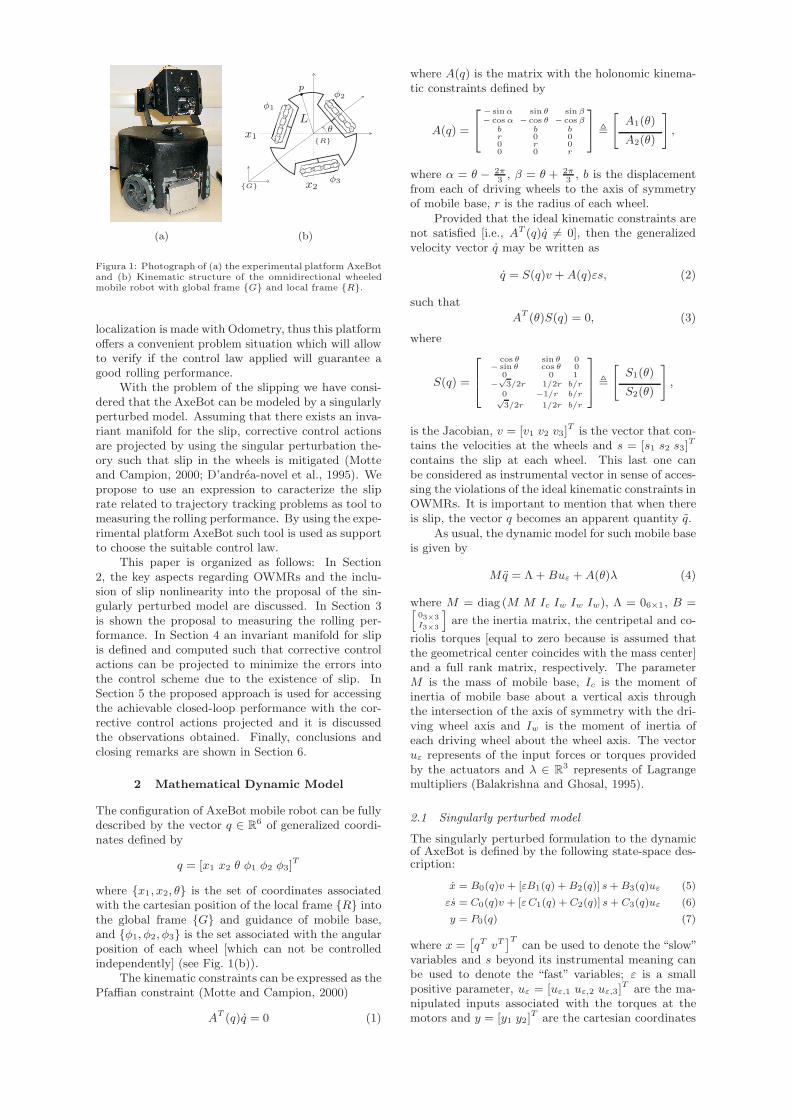
Figura 2: Trajectory tracking for a circle reference. Ini-tial pose: x1,0 = 0m,x2,0 = −0.12m,θ0 = 0 rad (y1,0 =0m, y2,0 = 0m).

−5

0

5

x 10−3

−0.02

−0.01

0

0.01

0.02−1

0

1

u0 + ε u

1

u0

u0 + ε u

1 + ε2 u

2

s1

s2

s3

Figura 3: Behavior of s around the rolling condition s =(0, 0, 0).

than 0.1) the derivatives dsidµi

are approximated by η =

10/19. From Assumption 1, ε = 10−10 for D = 4×109

and G = 1010. The reference dynamic was defined byK1 = 23 I3×3 and K2 = 70 I3×3 which is a criticallydamped second-order system with poles at -19.38 and-3.61. The reference trajectory is a circle with radius1 m.

In this paper was used (16) and (17) as a way toobserving the rolling performance of mobile base atdifferent reference trajectories at experimental resultsand finally to choose the suitable control law.

5.1 Circular trajectory and discussion of results

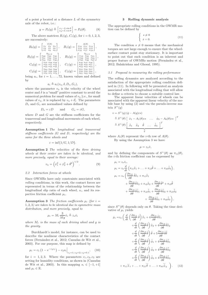
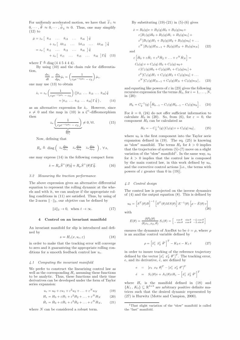
In Fig. 2 is shown the trajectory tracking of the circle.In Fig. 3 is shown the behavior of s around the con-dition s = (0, 0, 0). Clearly, the concentration of allpoints associated with this slip rate s are around theorigin (0,0,0). In the time domain the norm ‖s‖2 wasused as a way of understanding the total behavior ofslip into the overall dynamic of Axebot (see Fig. 4).The behavior observed at Fig. 4 show that the appro-priate rolling condition s = 0 defined by (11) has abehavior more near to zero when used the control lawwith two corrective control actions [i.e., u0+εu1+ε2u2](see the inset at Fig. 4). The other condition s 6= 0is a direct consequence of the behavior of norm ‖s‖when t → ∞. To explain this, one can proof thatthe kinematic constraints are not ever satisfied, i.e.AT (q)q 6= 0.

From observations in Fig. 4 we can affirm that‖s‖ → 0 for t → ∞. Consequently, limt→∞ s = 0

0 10 20 30 40 500

20

40

60

80

100

120

140

u0

u0 + ε u

1

u0 + ε u

1 +ε2 u

2

7 8 9 10 11 12

0

0.05

0.1

0.15

t(s)

‖s‖

Rolling Performance

Figura 4: Evolution of the norm ‖s‖ on time domain. Forsmall values of longitudinal slip (less than 0.1) the derivativesdsidµi

into the term Rµ were approximated by η = 10/19.

and limt→∞ s > 0, or limt→∞ s < 0, or limt→∞ s = 0.Multiplying both sides of (2) by AT (θ) yields

AT (θ)q = AT (θ)S(θ)v + AT (θ)A(θ)εs

= AT (θ)A(θ)εs (By using (3)) (29)

and since the model (5)-(7) assume that the kine-matic constraints are not satisfied [i.e., AT (q)q 6= 0and ε 6= 0], then can be verified that the optionlimt→∞ s = 0 contradize this assumption when suchoption is substituted in (29). Thus

limt→∞

s 6= 0

and we have proved the satisfaction of the appropriaterolling condition s 6= 0.

6 Final remarks

Here, we used an alternative expression for the rollingin an omnidirectional robot [the AxeBot] to observingthe slip behavior around the appropriate rolling con-ditions, s = 0 and s 6= 0. Considering the slip as afast variable within the overall dynamic of the mobilerobot is proposed a model based on theory of singularperturbations and consequently projected correctivecontrol actions that mitigate the influence of the slip.The AxeBot has a mechanism of self-localization in theworkspace based on odometry, thus the AxeBot giveus a convenient problem-situation to testing problemsarising from the presence of slip at the wheels. Withthe experimental information associated with the tra-jectory tracking is used the norm of the slip rate defi-ned by (16) as support to choosing what is the suitablecontrol law.

Currently, the methodology presented in this pa-per will be extended for wheeled mobile robots withnonholonomic and quasi-holonomic kinematic cons-traints that have controllers based in others theore-tical approaches different of the singular perturbationtheory.

Agradecimentos

The authors would like to thank Conselho Nacionalde Desenvolvimento Cientıfico e Tecnologico (CNPq),Coordenacao de Aperfeicoamento de Pessoal de Nıvel

Superior (CAPES), and Fundacao de Amparo a Pes-quisa do Estado da Bahia (FAPESB), all of them ofBrazil, for the research grant, financial support andstudy fellowship.

Referencias

Bahari, N., Becker, M. and Firouzi, H. (2008). Fea-ture based localization in an indoor environmentfor a mobile robot based on odometry, laser, andpanoramic vision data, ABCM Symposium Seriesin Mechatronics, Vol. 3, Rio de Janeiro, Brazil,pp. 266 – 275.

Balakrishna, R. and Ghosal, A. (1995). Modeling ofslip for wheeled mobile robots, IEEE Transacti-ons on Robotics and Automation 11(1): 126–132.

Canudas de Wit, C., Tsiotras, P., Velenis, E., Bas-set, M. and Gissinger, G. (2003). Dynamic fric-tion models for road/tire longitudinal interac-tion, Vehicle System Dynamics 39(3): 189–226.

D’andrea-novel, B., Campion, G. and Bastin, G.(1995). Control of wheeled mobile robots notsatisfying ideal velocity constraints: A singularperturbation approach, International Journal ofRobust and Nonlinear Control 5(4): 243–267.

Fernandez, C. A. P. and Cerqueira, J. J. F. (2009a).Control de velocidad con compensacion de desli-zamiento en las ruedas de una base holonomicausando un neurocontrolador basado en el modelonarma-l2, IX Congresso Brasileiro de Redes Neu-rais, Ouro Preto - Brasil.

Fernandez, C. A. P. and Cerqueira, J. J. F. (2009b).Identificacao de uma base holonomica para robosmoveis com escorregamento nas rodas usando ummodelo narmax polinomial, IX Simposio Brasi-leiro de Automacao Inteligente, Brasilia D.F -Brasil.

Fernandez, C. A. P., Cerqueira, J. J. F. and Lima, A.M. N. (2012). Dinamica nao-linear do escorre-gamento de um robo movel omnidirecional comrestricao de rolamento, XIX Congresso Brasileirode Automatica, Campina Grande - Brasil.

Ivankjo, E., Petrovic, I. and Vasak, M. (2004). Sonar-based pose tracking of indoor mobile robots,Journal for Control, Measurement, Electronics,Computing and Communications 45(3-4): 145–154.

Motte, I. and Campion, G. (2000). A slow manifoldapproach for the control of mobile robots not sa-tisfying the kinematic constraints, IEEE Tran-sactions on Robotics and Automation 16(6): 875–880.

Song, K.-T. and Wang, C.-W. (2009). Self-localizationand control of an omni-directional mobile robotbased on an omni-directional camera, Conf. Rec.IEEE/ASCC, Hong Kong, China, pp. 899 –904.

Trojnacki, M. (2013). Modeling and motion simulationof a three-wheeled mobile robot with front wheeldriven and steered taking into account wheelsslip, Archive of Applied Mechanics 83(1): 109–124.