Summarizing Data Due: Monday September 27, 2004

D:\web540w\docu\\extopic1

1

UNIVERSITY OF MASSACHUSETTS Department of Biostatistics and Epidemiology

BioEpi 540W - Introduction to Biostatistics Fall 2004

Exercises with Solutions– Topic 1

Summarizing Data

Due: Monday September 27, 2004 READINGS

1. Text (Rosner B. Fundamentals of Biostatistics, 5th Edition) Chapters 1 and 2. 2. Study Guide (Rosner B. Study Guide for Fundamentals of Biostatistics, 5th Edition)

Chapter 2.

EXERCISES: 1. For each of the following variables indicate whether it is quantitative or qualitative and

specify the measurement scale that is employed when taking measurements on each: (source: Daniel, page 12, problem #6.)

a) Class standing of members of this class relative to each other b) Admitting diagnosis of patients admitted to a mental health clinic c) Weights of babies born in a hospital during a year d) Gender of babies born in a hospital during a year e) Range of motion of elbow joint of students enrolled in a university health sciences

curriculum f) Under-arm temperature of day-old infants born in a hospital


2

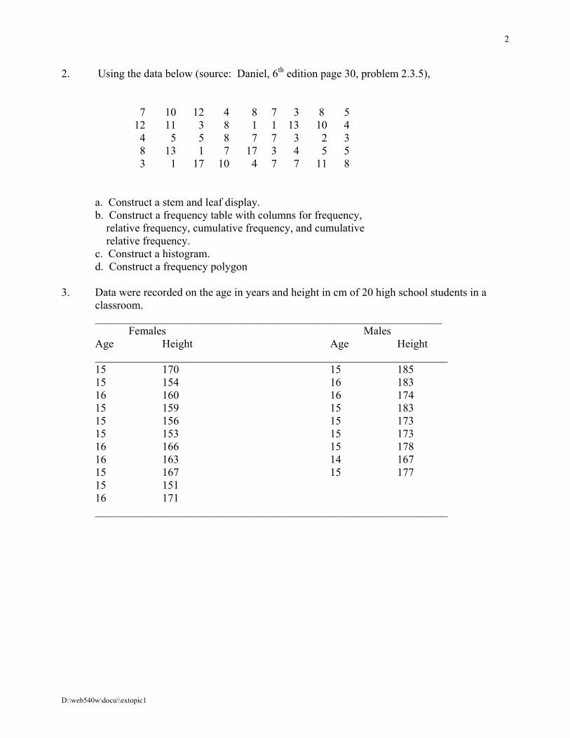
2. Using the data below (source: Daniel, 6th edition page 30, problem 2.3.5), 7 10 12 4 8 7 3 8 5 12 11 3 8 1 1 13 10 4 4 5 5 8 7 7 3 2 3 8 13 1 7 17 3 4 5 5 3 1 17 10 4 7 7 11 8 a. Construct a stem and leaf display. b. Construct a frequency table with columns for frequency, relative frequency, cumulative frequency, and cumulative relative frequency. c. Construct a histogram. d. Construct a frequency polygon 3. Data were recorded on the age in years and height in cm of 20 high school students in a

classroom. ______________________________________________________________ Females Males Age Height Age Height _______________________________________________________________ 15 170 15 185 15 154 16 183 16 160 16 174 15 159 15 183 15 156 15 173 15 153 15 173 16 166 15 178 16 163 14 167 15 167 15 177 15 151 16 171 _______________________________________________________________


3

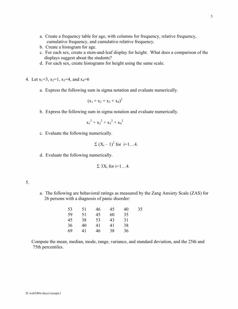
a. Create a frequency table for age, with columns for frequency, relative frequency, cumulative frequency, and cumulative relative frequency. b. Create a histogram for age. c. For each sex, create a stem-and-leaf display for height. What does a comparison of the displays suggest about the students? d. For each sex, create histograms for height using the same scale.

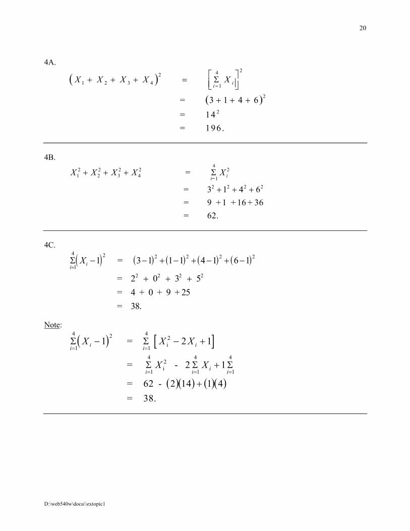
4. Let x1=3, x2=1, x3=4, and x4=6 a. Express the following sum in sigma notation and evaluate numerically. (x1 + x2 + x3 + x4)2

b. Express the following sum in sigma notation and evaluate numerically. x1

2 + x22 + x3

2 + x42

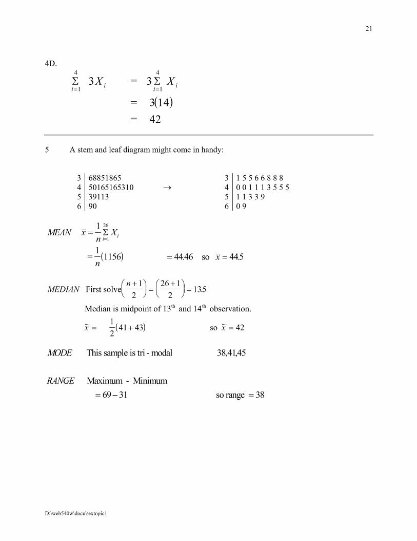
c. Evaluate the following numerically. Σ (Xi – 1)2 for i=1…4. d. Evaluate the following numerically. Σ 3Xi for i=1…4. 5. a. The following are behavioral ratings as measured by the Zang Anxiety Scale (ZAS) for 26 persons with a diagnosis of panic disorder: 53 51 46 45 40 35 59 51 45 60 35 45 38 53 43 31 36 40 41 41 38 69 41 46 38 36 Compute the mean, median, mode, range, variance, and standard deviation, and the 25th and 75th percentiles.


4

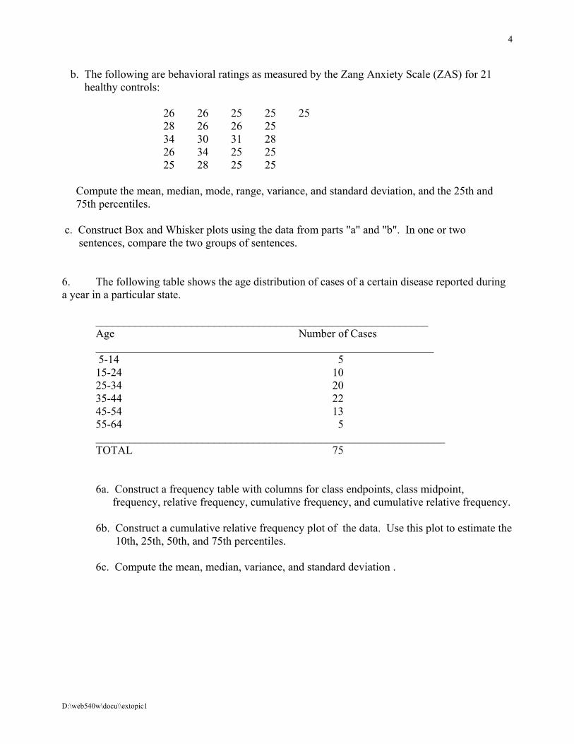
b. The following are behavioral ratings as measured by the Zang Anxiety Scale (ZAS) for 21 healthy controls: 26 26 25 25 25 28 26 26 25 34 30 31 28 26 34 25 25 25 28 25 25 Compute the mean, median, mode, range, variance, and standard deviation, and the 25th and 75th percentiles. c. Construct Box and Whisker plots using the data from parts "a" and "b". In one or two sentences, compare the two groups of sentences. 6. The following table shows the age distribution of cases of a certain disease reported during a year in a particular state. ___________________________________________________________ Age Number of Cases ____________________________________________________________ 5-14 5 15-24 10 25-34 20 35-44 22 45-54 13 55-64 5 ______________________________________________________________ TOTAL 75 6a. Construct a frequency table with columns for class endpoints, class midpoint, frequency, relative frequency, cumulative frequency, and cumulative relative frequency. 6b. Construct a cumulative relative frequency plot of the data. Use this plot to estimate the 10th, 25th, 50th, and 75th percentiles. 6c. Compute the mean, median, variance, and standard deviation .


5

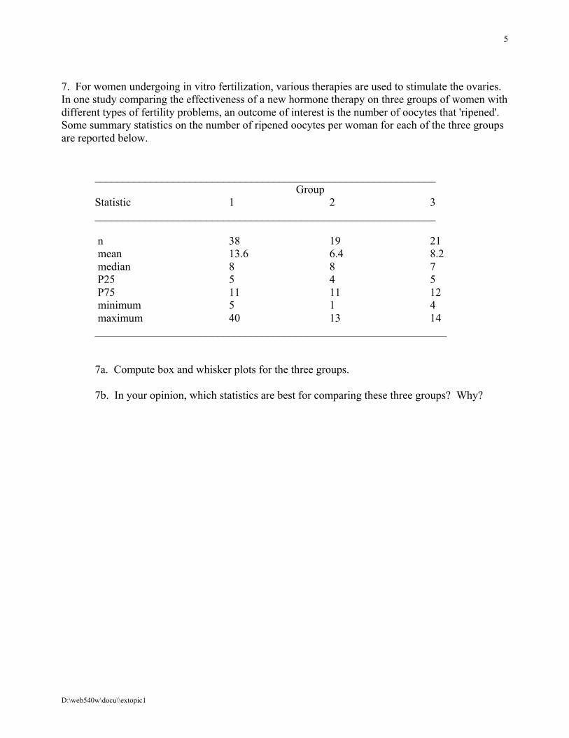
7. For women undergoing in vitro fertilization, various therapies are used to stimulate the ovaries. In one study comparing the effectiveness of a new hormone therapy on three groups of women with different types of fertility problems, an outcome of interest is the number of oocytes that 'ripened'. Some summary statistics on the number of ripened oocytes per woman for each of the three groups are reported below. _____________________________________________________________ Group Statistic 1 2 3 _____________________________________________________________ n 38 19 21 mean 13.6 6.4 8.2 median 8 8 7 P25 5 4 5 P75 11 11 12 minimum 5 1 4 maximum 40 13 14 _______________________________________________________________ 7a. Compute box and whisker plots for the three groups. 7b. In your opinion, which statistics are best for comparing these three groups? Why?


6

SOLUTIONS

#1.

a. Qualitative - ordinal b. Qualitative - nominal c. Quantitative - ratio d. Qualitative - nominal e. Quantitative - ratio f. Quantitative - interval

#2. How to Create a STATISTIX Data Set Containing This Information

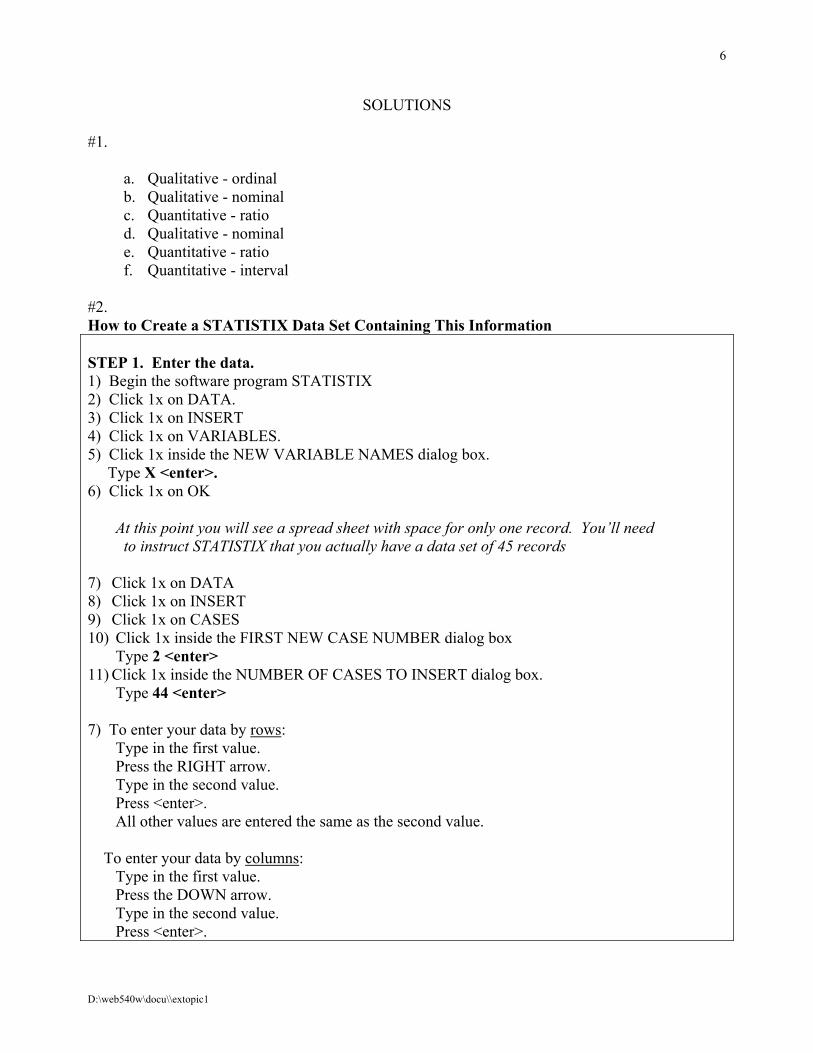
STEP 1. Enter the data. 1) Begin the software program STATISTIX 2) Click 1x on DATA. 3) Click 1x on INSERT 4) Click 1x on VARIABLES. 5) Click 1x inside the NEW VARIABLE NAMES dialog box. Type X <enter>. 6) Click 1x on OK At this point you will see a spread sheet with space for only one record. You’ll need to instruct STATISTIX that you actually have a data set of 45 records 7) Click 1x on DATA 8) Click 1x on INSERT 9) Click 1x on CASES 10) Click 1x inside the FIRST NEW CASE NUMBER dialog box

Type 2 <enter> 11) Click 1x inside the NUMBER OF CASES TO INSERT dialog box.

Type 44 <enter> 7) To enter your data by rows: Type in the first value. Press the RIGHT arrow. Type in the second value. Press <enter>. All other values are entered the same as the second value. To enter your data by columns: Type in the first value. Press the DOWN arrow. Type in the second value. Press <enter>.


7

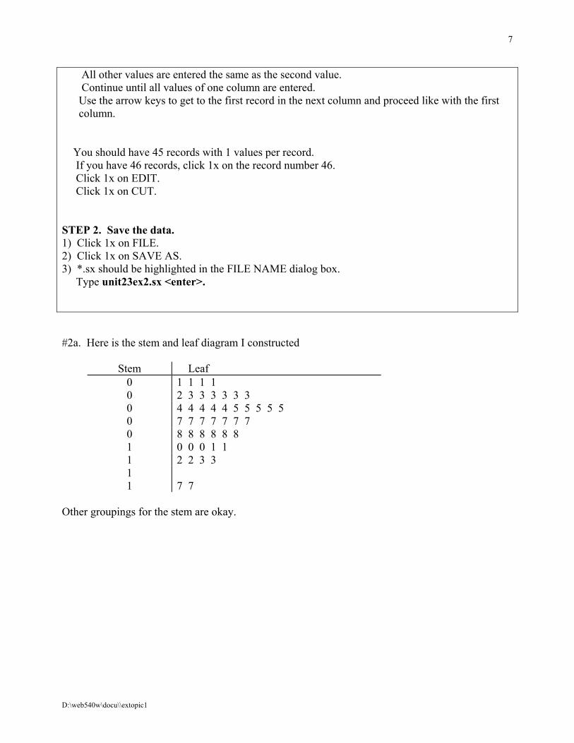
All other values are entered the same as the second value. Continue until all values of one column are entered. Use the arrow keys to get to the first record in the next column and proceed like with the first column.

You should have 45 records with 1 values per record. If you have 46 records, click 1x on the record number 46. Click 1x on EDIT. Click 1x on CUT. STEP 2. Save the data. 1) Click 1x on FILE. 2) Click 1x on SAVE AS. 3) *.sx should be highlighted in the FILE NAME dialog box. Type unit23ex2.sx <enter>. #2a. Here is the stem and leaf diagram I constructed

Stem Leaf 0 1 1 1 1 0 2 3 3 3 3 3 3 0 4 4 4 4 4 5 5 5 5 5 0 7 7 7 7 7 7 7 0 8 8 8 8 8 8 1 0 0 0 1 1 1 2 2 3 3 1 1 7 7

Other groupings for the stem are okay.


8

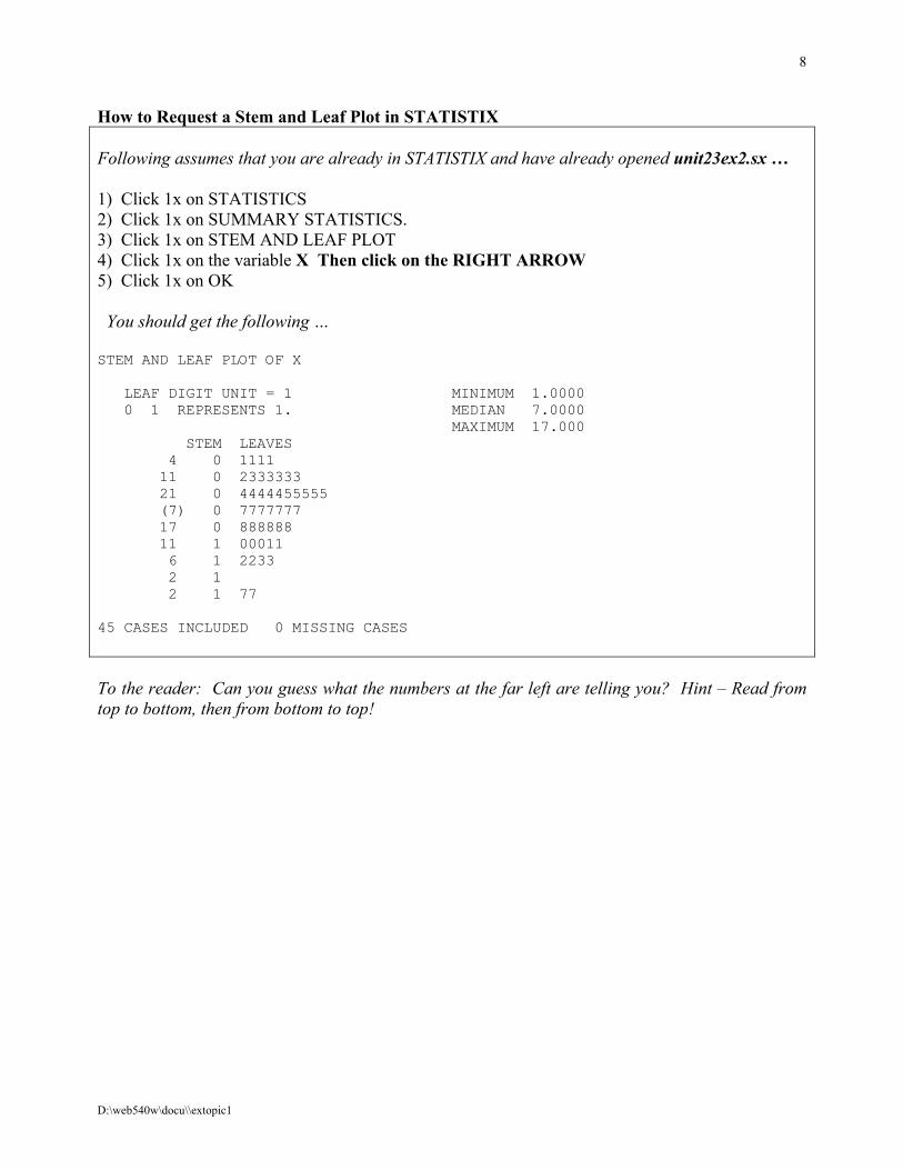
How to Request a Stem and Leaf Plot in STATISTIX Following assumes that you are already in STATISTIX and have already opened unit23ex2.sx … 1) Click 1x on STATISTICS 2) Click 1x on SUMMARY STATISTICS. 3) Click 1x on STEM AND LEAF PLOT 4) Click 1x on the variable X Then click on the RIGHT ARROW 5) Click 1x on OK You should get the following … STEM AND LEAF PLOT OF X LEAF DIGIT UNIT = 1 MINIMUM 1.0000 0 1 REPRESENTS 1. MEDIAN 7.0000 MAXIMUM 17.000 STEM LEAVES 4 0 1111 11 0 2333333 21 0 4444455555 (7) 0 7777777 17 0 888888 11 1 00011 6 1 2233 2 1 2 1 77 45 CASES INCLUDED 0 MISSING CASES To the reader: Can you guess what the numbers at the far left are telling you? Hint – Read from top to bottom, then from bottom to top!


9

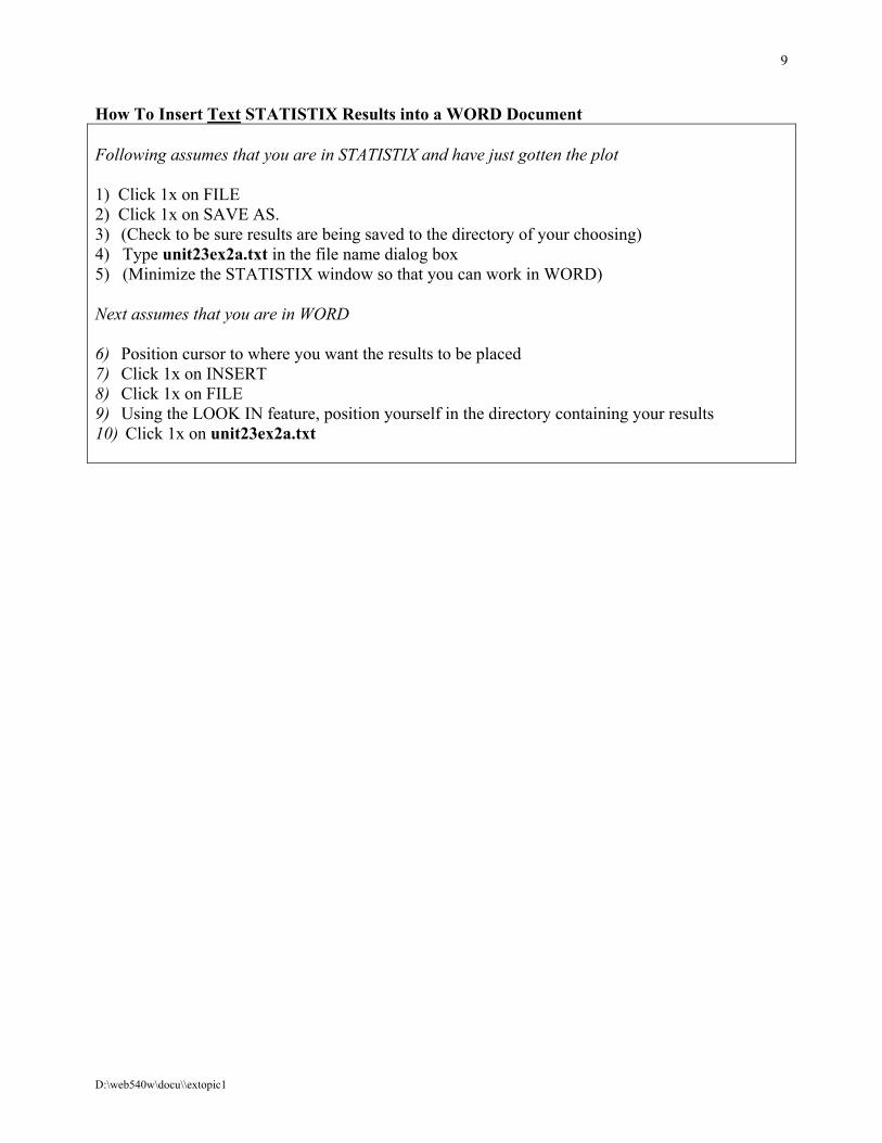
How To Insert Text STATISTIX Results into a WORD Document Following assumes that you are in STATISTIX and have just gotten the plot 1) Click 1x on FILE 2) Click 1x on SAVE AS. 3) (Check to be sure results are being saved to the directory of your choosing) 4) Type unit23ex2a.txt in the file name dialog box 5) (Minimize the STATISTIX window so that you can work in WORD) Next assumes that you are in WORD 6) Position cursor to where you want the results to be placed 7) Click 1x on INSERT 8) Click 1x on FILE 9) Using the LOOK IN feature, position yourself in the directory containing your results 10) Click 1x on unit23ex2a.txt


10

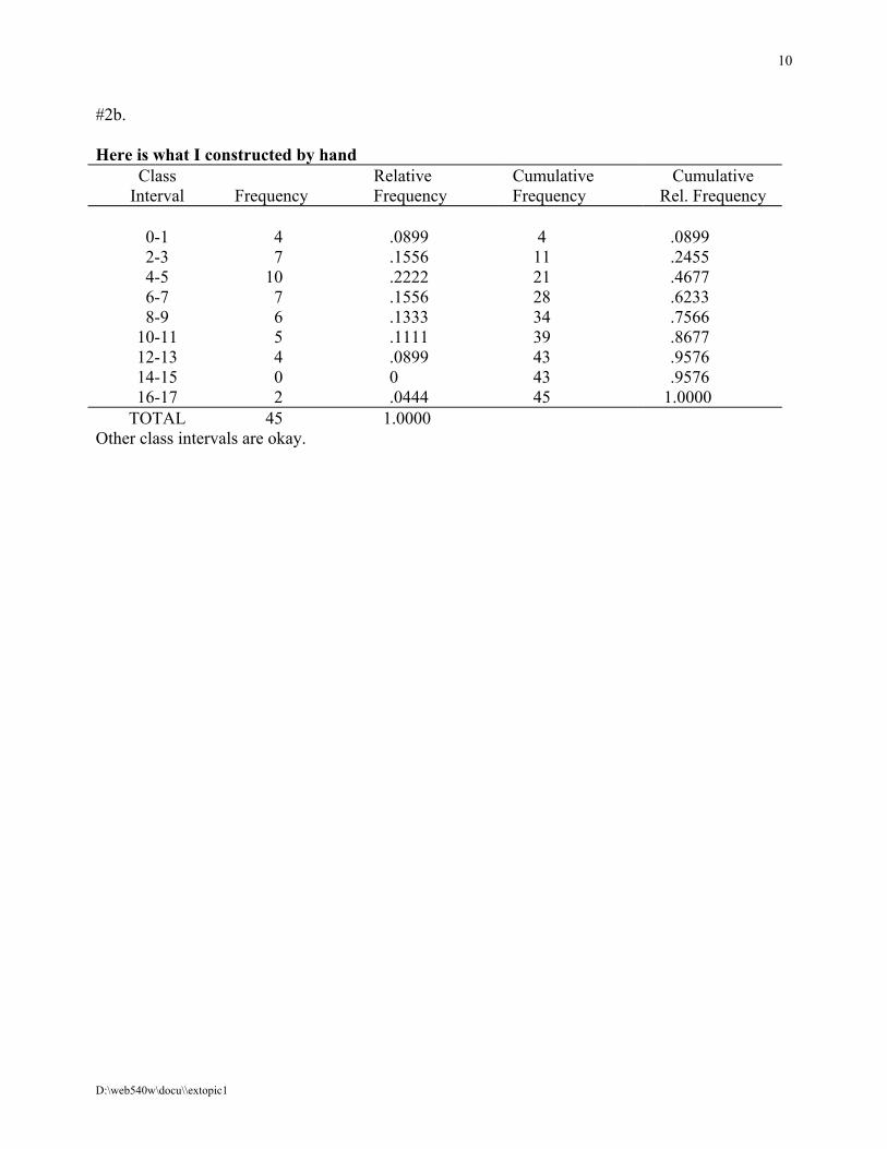
#2b. Here is what I constructed by hand

Class Relative Cumulative Cumulative Interval Frequency Frequency Frequency Rel. Frequency

0-1 4 .0899 4 .0899 2-3 7 .1556 11 .2455 4-5 10 .2222 21 .4677 6-7 7 .1556 28 .6233 8-9 6 .1333 34 .7566

10-11 5 .1111 39 .8677 12-13 4 .0899 43 .9576 14-15 0 0 43 .9576 16-17 2 .0444 45 1.0000

TOTAL 45 1.0000 Other class intervals are okay.


11

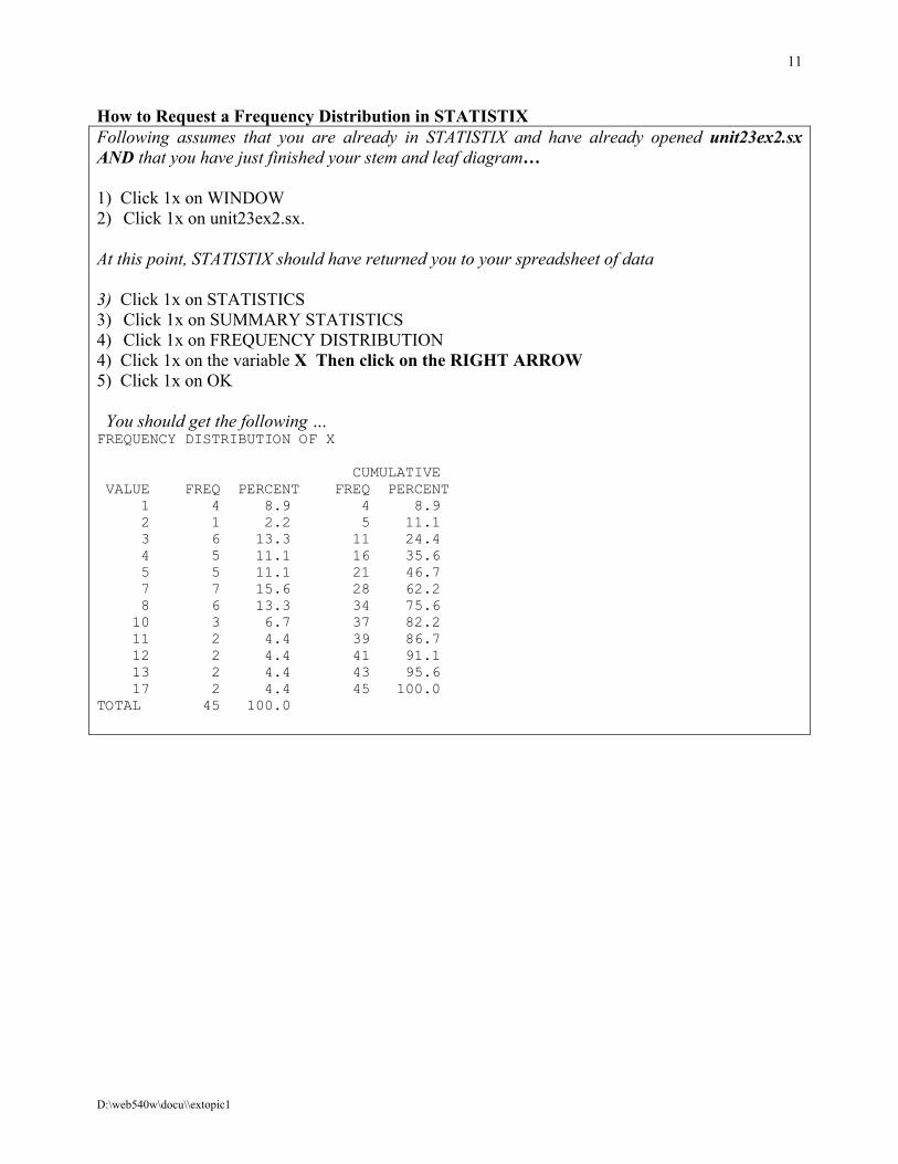
How to Request a Frequency Distribution in STATISTIX Following assumes that you are already in STATISTIX and have already opened unit23ex2.sx AND that you have just finished your stem and leaf diagram… 1) Click 1x on WINDOW 2) Click 1x on unit23ex2.sx. At this point, STATISTIX should have returned you to your spreadsheet of data 3) Click 1x on STATISTICS 3) Click 1x on SUMMARY STATISTICS 4) Click 1x on FREQUENCY DISTRIBUTION 4) Click 1x on the variable X Then click on the RIGHT ARROW 5) Click 1x on OK You should get the following … FREQUENCY DISTRIBUTION OF X CUMULATIVE VALUE FREQ PERCENT FREQ PERCENT 1 4 8.9 4 8.9 2 1 2.2 5 11.1 3 6 13.3 11 24.4 4 5 11.1 16 35.6 5 5 11.1 21 46.7 7 7 15.6 28 62.2 8 6 13.3 34 75.6 10 3 6.7 37 82.2 11 2 4.4 39 86.7 12 2 4.4 41 91.1 13 2 4.4 43 95.6 17 2 4.4 45 100.0 TOTAL 45 100.0


12

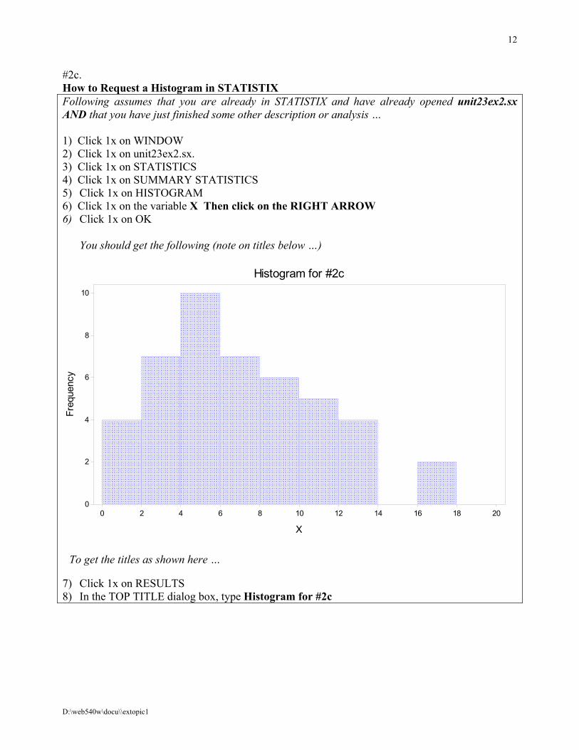
#2c. How to Request a Histogram in STATISTIX Following assumes that you are already in STATISTIX and have already opened unit23ex2.sx AND that you have just finished some other description or analysis … 1) Click 1x on WINDOW 2) Click 1x on unit23ex2.sx. 3) Click 1x on STATISTICS 4) Click 1x on SUMMARY STATISTICS 5) Click 1x on HISTOGRAM 6) Click 1x on the variable X Then click on the RIGHT ARROW 6) Click 1x on OK

You should get the following (note on titles below …)

0 2 4 6 8 10 12 14 16 18 200

2

4

6

8

10

Histogram for #2c

Freq

uenc

y

X

To get the titles as shown here … 7) Click 1x on RESULTS 8) In the TOP TITLE dialog box, type Histogram for #2c


13

How To Insert GRAPHICAL STATISTIX Results into a WORD Document Following assumes that you are in STATISTIX and have just gotten the plot 1) Click 1x on FILE 2) Click 1x on SAVE AS. 4) (Check to be sure results are being saved to the directory of your choosing) 4) Type unit23ex2c.emf in the file name dialog box 5) (Minimize the STATISTIX window so that you can work in WORD) Next assumes that you are in WORD 6) Position cursor to where you want the results to be placed 7) Click 1x on INSERT 8) Click 1x on PICTURE 9) Click 1x on FROM FILE 10) Using the LOOK IN feature, position yourself in the directory containing your results 11) Click 1x on unit23ex2c.emf


14

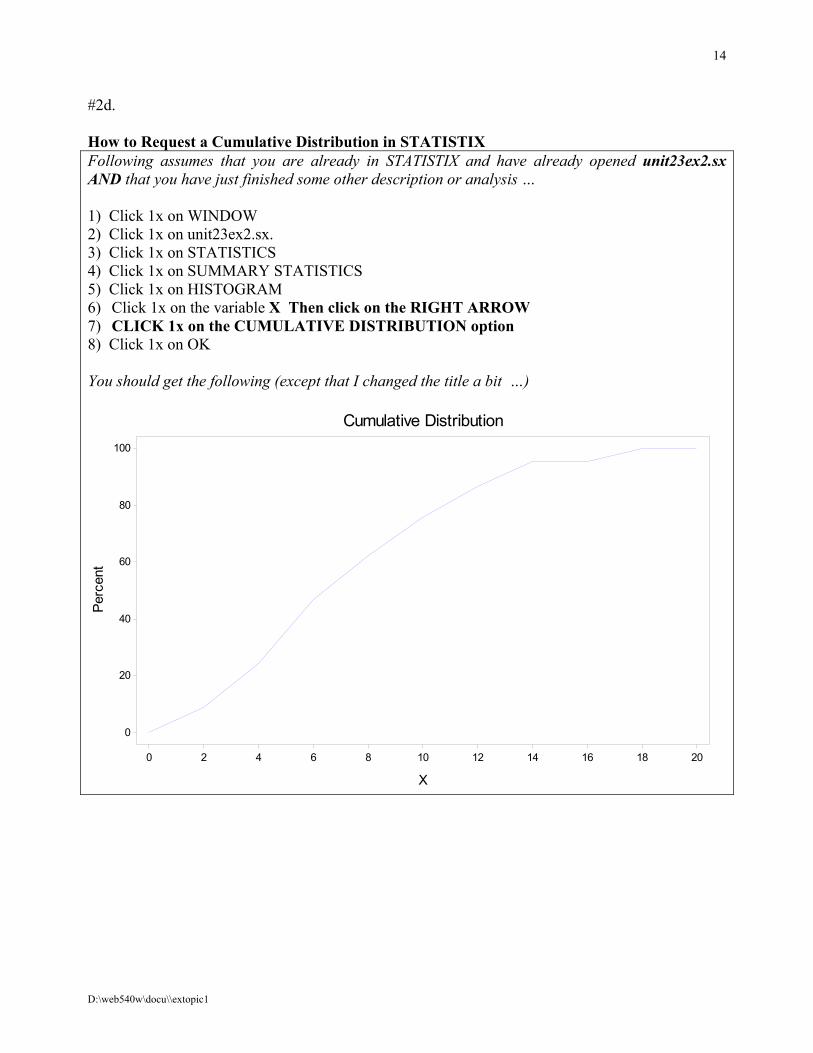
#2d. How to Request a Cumulative Distribution in STATISTIX Following assumes that you are already in STATISTIX and have already opened unit23ex2.sx AND that you have just finished some other description or analysis … 1) Click 1x on WINDOW 2) Click 1x on unit23ex2.sx. 3) Click 1x on STATISTICS 4) Click 1x on SUMMARY STATISTICS 5) Click 1x on HISTOGRAM 6) Click 1x on the variable X Then click on the RIGHT ARROW 7) CLICK 1x on the CUMULATIVE DISTRIBUTION option 8) Click 1x on OK You should get the following (except that I changed the title a bit …)

0 2 4 6 8 10 12 14 16 18 20

0

20

40

60

80

100

Cumulative Distribution

Perc

ent

X


15

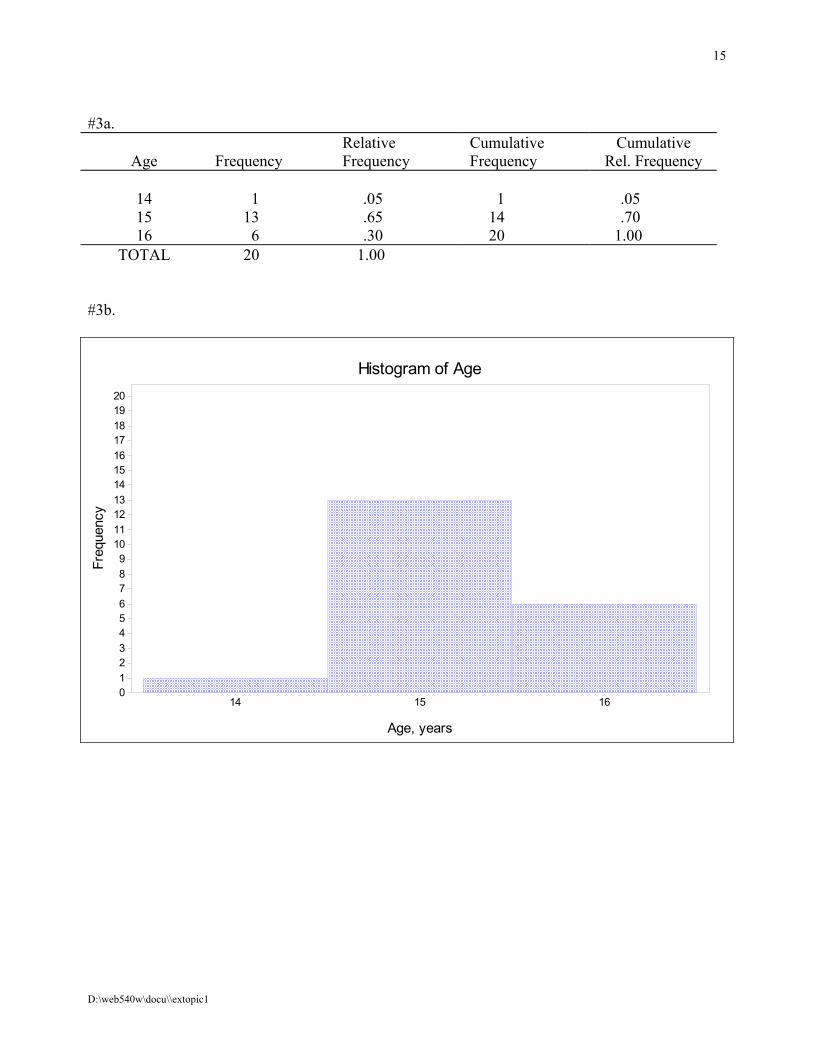
#3a.

Relative Cumulative Cumulative Age Frequency Frequency Frequency Rel. Frequency

14 1 .05 1 .05 15 13 .65 14 .70 16 6 .30 20 1.00

TOTAL 20 1.00 #3b.

14 15 160123456789

1011121314151617181920

Histogram of Age

Freq

uenc

y

Age, years


16

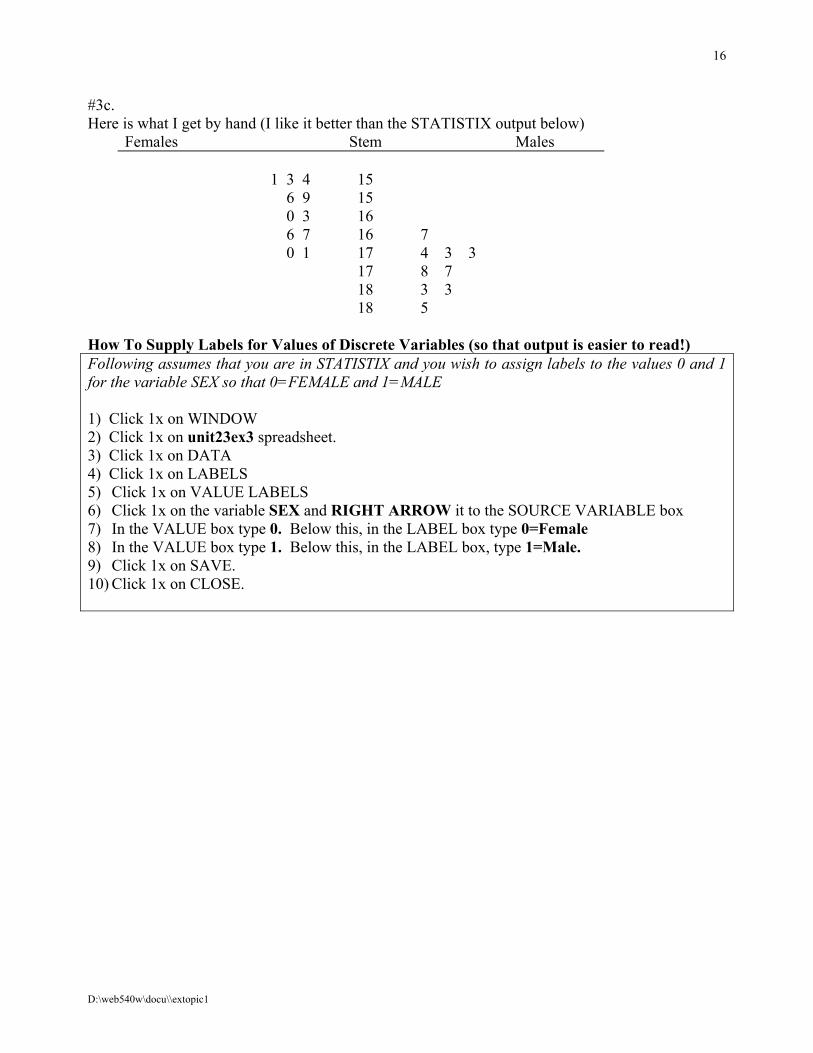
#3c. Here is what I get by hand (I like it better than the STATISTIX output below)

Females Stem Males

1 3 4 15 6 9 15 0 3 16 6 7 16 7 0 1 17 4 3 3

17 8 7 18 3 3 18 5

How To Supply Labels for Values of Discrete Variables (so that output is easier to read!) Following assumes that you are in STATISTIX and you wish to assign labels to the values 0 and 1 for the variable SEX so that 0=FEMALE and 1=MALE 1) Click 1x on WINDOW 2) Click 1x on unit23ex3 spreadsheet. 3) Click 1x on DATA 4) Click 1x on LABELS 5) Click 1x on VALUE LABELS 6) Click 1x on the variable SEX and RIGHT ARROW it to the SOURCE VARIABLE box 7) In the VALUE box type 0. Below this, in the LABEL box type 0=Female 8) In the VALUE box type 1. Below this, in the LABEL box, type 1=Male. 9) Click 1x on SAVE. 10) Click 1x on CLOSE.


17

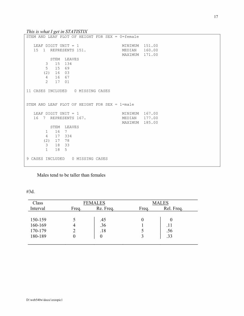
This is what I get in STATISTIX STEM AND LEAF PLOT OF HEIGHT FOR SEX = 0=female LEAF DIGIT UNIT = 1 MINIMUM 151.00 15 1 REPRESENTS 151. MEDIAN 160.00 MAXIMUM 171.00 STEM LEAVES 3 15 134 5 15 69 (2) 16 03 4 16 67 2 17 01 11 CASES INCLUDED 0 MISSING CASES STEM AND LEAF PLOT OF HEIGHT FOR SEX = 1=male LEAF DIGIT UNIT = 1 MINIMUM 167.00 16 7 REPRESENTS 167. MEDIAN 177.00 MAXIMUM 185.00 STEM LEAVES 1 16 7 4 17 334 (2) 17 78 3 18 33 1 18 5 9 CASES INCLUDED 0 MISSING CASES Males tend to be taller than females #3d.

Class FEMALES MALES Interval Freq. Re. Freq. Freq. Rel. Freq. 150-159 5 .45 0 0 160-169 4 .36 1 .11 170-179 2 .18 5 .56 180-189 0 0 3 .33


18

How To Select A Subset of the Data for Analysis We wish to construct separate histograms, first for females, then for males. STATISTIX is a bit awkward in this. To Select Females, STATISTIX requires that you omit Males 1) Click 1x on WINDOW 2) Click 1x on unit23ex3 spreadsheet. 3) Click 1x on DATA 4) Click 1x on OMIT/SELECT/RESTORE CASES 5) Type Omit sex=1 6) Click 1x on GO 7) Click 1x on CLOSE Construct your histogram using instructions per above. Take care to title it clearly. Before you can select males, you must restore the entire data set 1) Click 1x on WINDOW 2) Click 1x on unit23ex3 spreadsheet 3) Click 1x on OMIT/SELECT/RESTORE CASES 4) Type restore To Select Males, STATISTIX requires that you omit Females 1) Type Omit sex=0 2) Click 1x on GO 3) Click 1x on CLOSE


19

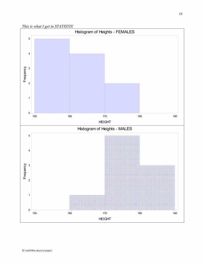
This is what I get in STATISTIX

150 160 170 180 1900

1

2

3

4

5

Histogram of Heights - FEMALES

Freq

uenc

y

HEIGHT

150 160 170 180 1900

1

2

3

4

5

Histogram of Heights - MALES

Freq

uenc

y

HEIGHT


20

4A.

( )( )

X X X X Xi i1 2 3 4

2

1

4 2

23 1 4 6

+ + + =

+ + +

=

= = 14 = 196 .

2

Σ

4B.

X X X X Xi= i1

222

32

42

1

42

2 2 21 4 6

+ + +

+ + +

=

= 3 = 9 + 1 + 16 + 36 = 62.

2

Σ

4C.

( ) ( ) ( ) ( ) ( )Σi iX=

− − + − + − + −

+ + +1

4 2 2 2 2 2

2 2 2

1 3 1 1 1 4 1 6 1

0 3 5

=

= 2 = 4 + 0 + 9 + 25 = 38.

2

Note:

( ) [ ]

( )( ) ( )( )

Σ Σ

Σ Σ Σ

i i i i

i i i i

X X X

X X

= =

= = =

− − +

+

+

1

4 2

1

4

1

4

1

4

1

4

1 2 1

1

14 1 4

=

= - 2

= 62 - 2 = 38.

i2

i2


21

4D.

( )

Σ Σi i i iX X= =1

4

1

43 = 3

= 3 14 = 42

5 A stem and leaf diagram might come in handy:

3 68851865 3 1 5 5 6 6 8 8 8 4 50165165310 → 4 0 0 1 1 1 3 5 5 5 5 39113 5 1 1 3 3 9 6 90 6 0 9

( )

MEAN xn

X

=n

x

i i

so

=

= =

=

1

11156 4446 445

1

26Σ

. .

( )

MEDIANn

x x

First solve

Median is midpoint of 13 and 14 observation.

so

th th

+

=

+

=

= + =

12

26 12

135

12

41 43 42

.

~ ~

MODE

RANGE

This sample is tri - modal

Maximum - Minimum so range

38 4145

69 31 38

, ,

= − =


22

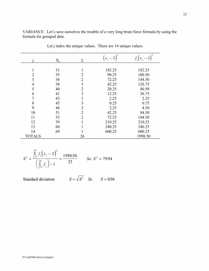
VARIANCE Let’s save ourselves the trouble of a very long brute force formula by using the formula for grouped data. Let j index the unique values. There are 14 unique values.

j

Xj

fj ( )x xj −

2 ( )f x xj j −

2

1 31 1 182.25 182.25 2 35 2 90.25 180.50 3 36 2 72.25 144.50 4 38 3 42.25 126.75 5 40 2 20.25 40.50 6 41 3 12.25 36.75 7 43 1 2.25 2.25 8 45 3 0.25 0.75 9 46 2 2.25 4.50 10 51 2 42.25 84.50 11 53 2 72.25 144.50 12 59 1 210.25 210.25 13 60 1 240.25 240.25 14 69 1 600.25 600.25

TOTALS 26 1998.50

( )S

f x x

fSo Sj j j

j j

2 1

14 2

1

142

1

1998 5025

79 94=−

−

= ==

=

Σ

Σ

..

Standard deviation S S So S= =2 894.


23

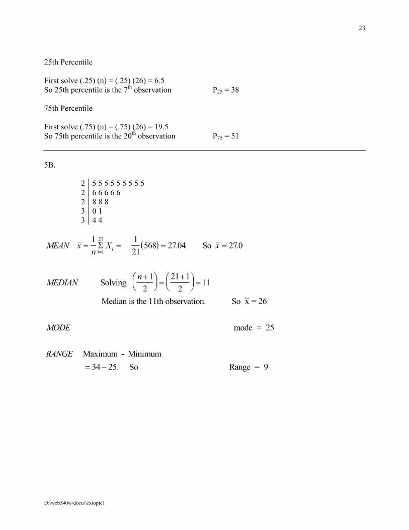
25th Percentile First solve (.25) (n) = (.25) (26) = 6.5 So 25th percentile is the 7th observation P25 = 38 75th Percentile First solve (.75) (n) = (.75) (26) = 19.5 So 75th percentile is the 20th observation P75 = 51 5B.

2 5 5 5 5 5 5 5 5 5 2 6 6 6 6 6 2 8 8 8 3 0 1 3 4 4

( )MEAN xn

X x

MEDIANn

MODE

RANGE

i i So

Solving

Median is the 11th observation. So x = 26

mode = 25

Maximum - Minimum So Range = 9

= = = =

+

=

+

=

= −

=

1 121

568 2704 270

12

21 12

11

34 25

1

21Σ . .

~

.


24

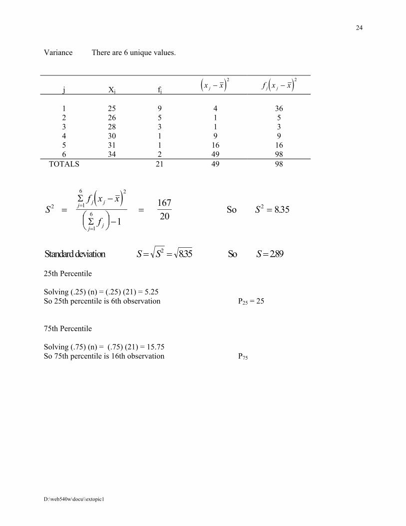
Variance There are 6 unique values.

j

Xj

fj ( )x xj −

2 ( )f x xj j −

2

1 25 9 4 36 2 26 5 1 5 3 28 3 1 3 4 30 1 9 9 5 31 1 16 16 6 34 2 49 98

TOTALS 21 49 98

( )S

f x x

fSj j j

j j

2 1

6 2

1

62

1

16720

835 So =−

−

= ==

=

Σ

Σ.

Standard deviation So S S S= = =2 835 289. . 25th Percentile Solving (.25) (n) = (.25) (21) = 5.25 So 25th percentile is 6th observation P25 = 25 75th Percentile Solving (.75) (n) = (.75) (21) = 15.75 So 75th percentile is 16th observation P75


25

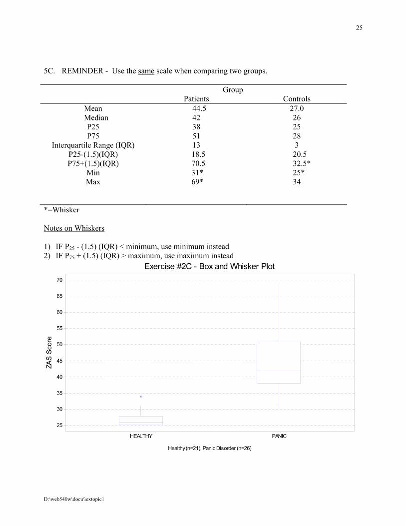
5C. REMINDER - Use the same scale when comparing two groups.

Group Patients Controls

Mean 44.5 27.0 Median 42 26

P25 38 25 P75 51 28

Interquartile Range (IQR) 13 3 P25-(1.5)(IQR) 18.5 20.5 P75+(1.5)(IQR) 70.5 32.5*

Min 31* 25* Max 69* 34

*=Whisker Notes on Whiskers 1) IF P25 - (1.5) (IQR) < minimum, use minimum instead 2) IF P75 + (1.5) (IQR) > maximum, use maximum instead Patients with panic disorder have ZAS scores that are higher than those of controls. As well, ZAS scores of patients with panic disorder have more variability.

HEALTHY PANIC

25

30

35

40

45

50

55

60

65

70

Exercise #2C - Box and Whisker Plot

ZAS

Scor

e

Healthy (n=21), Panic Disorder (n=26)


26

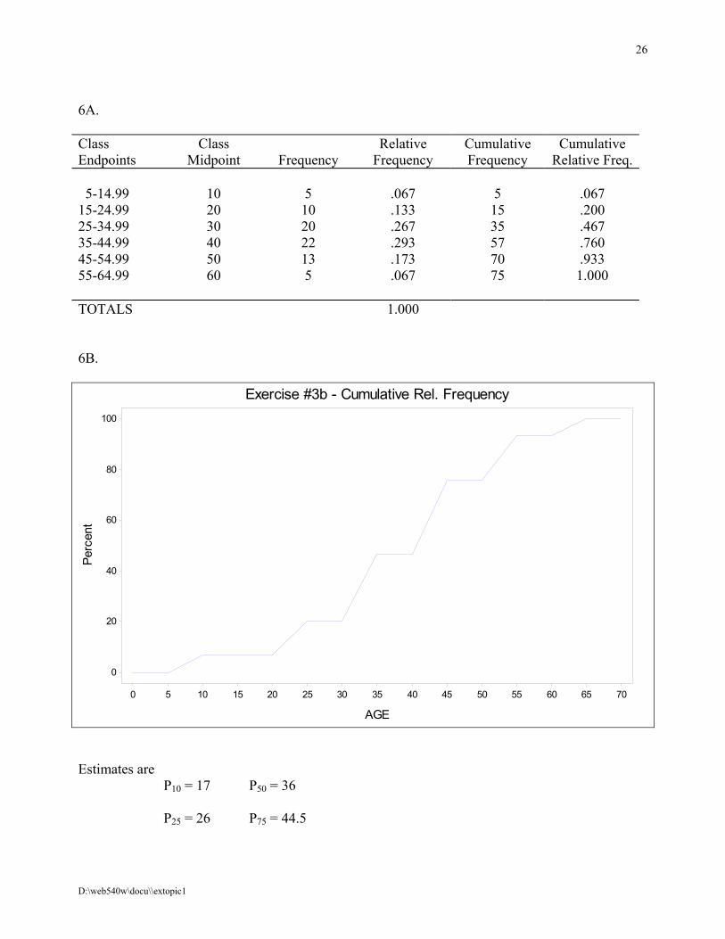
6A. Class Class Relative Cumulative Cumulative Endpoints Midpoint Frequency Frequency Frequency Relative Freq. 5-14.99 10 5 .067 5 .067 15-24.99 20 10 .133 15 .200 25-34.99 30 20 .267 35 .467 35-44.99 40 22 .293 57 .760 45-54.99 50 13 .173 70 .933 55-64.99 60 5 .067 75 1.000 TOTALS 1.000 6B.

0 5 10 15 20 25 30 35 40 45 50 55 60 65 70

0

20

40

60

80

100

Exercise #3b - Cumulative Rel. Frequency

Perc

ent

AGE

Estimates are P10 = 17 P50 = 36 P25 = 26 P75 = 44.5


27

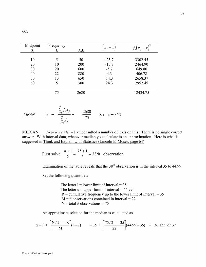
6C.

Midpoint Xj

Frequency fj

Xjfj

( )x xj − ( )f x xj j −2

10 5 50 -25.7 3302.45 20 10 200 -15.7 2464.90 30 20 600 -5.7 649.80 40 22 880 4.3 406.78 50 13 650 14.3 2658.37 60 5 300 24.3 2952.45 75 2680 12434.75

MEAN xf x

fxj j j

j j

So = = ==

=

Σ

Σ

1

6

1

6268075

357.

MEDIAN Note to reader – I’ve consulted a number of texts on this. There is no single correct answer. With interval data, whatever median you calculate is an approximation. Here is what is suggested in Think and Explain with Statistics (Lincoln E. Moses, page 64)

First solve observationn

th+

=+

=1

275 1

238

Examination of the table reveals that the 38th observation is in the interval 35 to 44.99 Set the following quantities: The letter l = lower limit of interval = 35 The letter u = upper limit of interval = 44.99 R = cumulative frequency up to the lower limit of interval = 35 M = # observations contained in interval = 22 N = total # observations = 75 An approximate solution for the median is calculated as

~ ( )x = + N / 2 - RM

l u lLNM

OQP − = 35 + 75 / 2 - 35

22LNM

OQP −( . )44 99 35 = 36.135 or 37


28

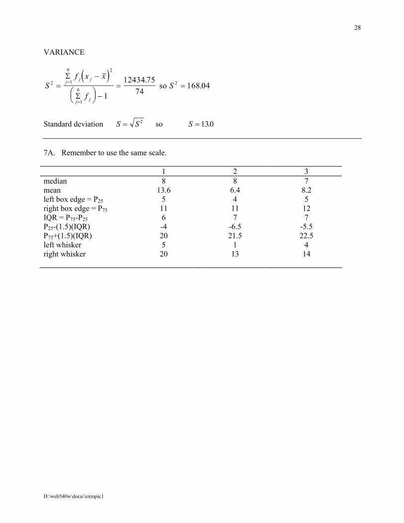
VARIANCE

( )S

f x x

fSj j j

j j

2 1

6 2

1

62

1

12434 7574

168 04=−

−

= ==

=

Σ

Σ

.. so

Standard deviation S S S= =2 130 so . 7A. Remember to use the same scale. 1 2 3 median 8 8 7 mean 13.6 6.4 8.2 left box edge = P25 5 4 5 right box edge = P75 11 11 12 IQR = P75-P25 6 7 7 P25-(1.5)(IQR) -4 -6.5 -5.5 P75+(1.5)(IQR) 20 21.5 22.5 left whisker 5 1 4 right whisker 20 13 14


29

7B. When data are skewed by extreme values, medians and quartiles give a better feel for the bulk of the data than do means and standard deviations. This example also illustrates that, as sample size increases, the range can only increase. Notice that the extreme value of 40 occurred in the sample with the largest sample size.

Documents

Summarizing Data Due: Monday September 27, 2004