UNIVERSITY OF KAISERSLAUTERN

Summarizing XML Documents:

Contributions, Empirical Studies,

and Challenges

by

Jose de Aguiar Moraes Filho

A thesis submitted in partial fulfillment for the

degree of Doktor der Ingenieurwissenschaften (Dr.-Ing.)

to the

Department of Computer Science

under the supervision ofProf. Dr.-Ing. Dr. h. c. Theo Harder

November 2009

Declaration of Authorship

I, Jose de Aguiar Moraes Filho, declare that this thesis titled ‘Summarizing XML

Documents: Contributions, Empirical Studies, and Challenges’ and the work pre-

sented in it are my own. I confirm that:

� This work was done wholly or mainly while in candidature for a research

degree at this University.

� Where any part of this thesis has previously been submitted for a degree or

any other qualification at this University or any other institution, this has

been clearly stated.

� Where I have consulted the published work of others, this is always clearly

attributed.

� Where I have quoted from the work of others, the source is always given.

With the exception of such quotations, this thesis is entirely my own work.

� I have acknowledged all main sources of help.

� Where the thesis is based on work done by myself jointly with others, I have

made clear exactly what was done by others and what I have contributed

myself.

Signed:

Date:

ii

Examination Board

1. Reviewer: Prof. Dr.-Ing. Dr. h. c. Theo Harder

2. Reviewer: Prof. Dr.-Ing. Angelo R. A. Brayner

Date of the defense:

Signature from the Head of PhD Committee:

iii

“Do you want to know how to shrink a tree? The answer is simple: Bonsai.”

UNIVERSITY OF KAISERSLAUTERN

Department of Computer Science

Databases and Information Systems Group (AG DBIS)

Summarizing XML Documents:

Contributions, Empirical Studies,

and Challengesby Jose de Aguiar Moraes Filho

Abstract

We tackle the problem of obtaining statistics on content and structure of XML

documents by using summaries which may provide cardinality estimations for

XML query expressions. Our focus is a data-centric processing scenario in which

we use a query engine to process such query expressions.

We provide three new summary structures called LESS (Leaf-Element-in-Subtree),

LWES (Level-Wide Element Summarization), and EXsum (Element-centered XML

Summarization) which are targeted to base an estimation process in an XML

query optimizer. Each of these collects structural statistical information of XML

documents, and the latter (EXsum) gathers, in addition, statistics on document

content. Estimation procedures and/or heuristics for specific types of query ex-

pressions of each proposed approach are developed.

We have incorporated and implemented our proposals in XTC, a native XML

database management system (XDBMS). With this common implementation base,

we present an empirical and comparative study in which our proposals are stressed

against others published in the literature, which are also incorporated into the

XTC. Furthermore, an analysis is made based on criteria pertinent to a query

optimizer process.

Subject: XML summarization

Keywords: XML summary, statistics, structural summary, content-and-structure

summary, XML query estimation

v

Acknowledgements

Acknowledgments are first due to my supervisor Prof. Dr.-Ing. Dr. h. c. Theo

Harder for the opportunity and support he gave me and whose firm, gentle, and

invaluable advisory has made it possible for me to fulfill this degree.

Thanks must be given to my (former) Master advisor, Prof. Dr.-Ingl. Angelo

Brayner for motivating me to go further and embark upon this enterprise called

PhD.

My company, SERPRO—Brazilian Federal Government Data Center—is similarly

acknowledged for the (partial) financial support throughout my pursuit of a doc-

toral degree. I would especially like to thank Carlos Augusto Neiva (Manager of

The Fortaleza Development Center), Aluysio Pinto (former SERPRO Superinten-

dent for SUNAF business area, until 2004), Myuki Abe (former SUNAF Superin-

tendent, succeeding Aluysio Pinto, from 2004 to 2006), Eunides Maria Chaves (for-

mer SERPRO Superintendent for Human Resources), Vera Lucia Moraes (SER-

PRO Corporative University), and Ana Sarah Holanda (Human Resources Chief

in Fortaleza). I would like to thank my colleagues on the SERPRO DBA team

in Fortaleza, for their best wishes for accomplishing this title. Marcos Camara de

Paula, member of the Fortaleza DBA team and actual chief of the DBAs is ac-

knowledged for his support for other personal matter issues during this time. To

the SERPRO administrative staff in Fortaleza (Laıs Colignac, Rosa Maria, Nilzete

Sampaio, and Angela Venancio) and to all my colleagues in SERPRO, whether

in Fortaleza or in Brasilia, I want to say: Thank you all, from the bottom of my

heart!

I also need to thank Caetano Sauer, Felipe Mobus, and Leonardo Dalpiaz for

helping me in the implementation phase of my work.

The scientific staff of AG DBIS is also acknowledged. I would like to cite the names

of Christian Mathis, Sebastian Bachle, Karsten Schmidt, and Andreas Weiner,

among others, who assisted me with issues related to the XTC project.

I offer my kind thanks to the administrative of AG DBIS, specifically, Lothar Gaus,

Manuela Burkart, and Steffen Reithermann for their day-by-day availability.

Last but not least, to all others who I may have failed to mention herein, who

have directly or indirectly contributed to this work being completed.

vi

To God, with Him everything is possible.

To my wife, Ana Lucia, for her patient love and care in dealing

with my absence while I worked on this project.

To my father, Jose de Aguiar Moraes, for being an example of

enduring adverse circumstances.

Contents

List of Figures xi

List of Tables xiii

List of Algorithms xiv

Abbreviations xv

1 Introduction 1

1.1 The Advent of XML and Semi-Structured Data . . . . . . . . . . . 1

1.1.1 XML—A Brief History . . . . . . . . . . . . . . . . . . . . . 3

1.1.2 XML-related Technologies . . . . . . . . . . . . . . . . . . . 3

1.1.3 The XML Document . . . . . . . . . . . . . . . . . . . . . . 4

1.1.4 Processing XML Documents . . . . . . . . . . . . . . . . . . 6

1.2 XML Data Management . . . . . . . . . . . . . . . . . . . . . . . . 7

1.2.1 Identifying Document Nodes . . . . . . . . . . . . . . . . . . 8

1.2.2 Querying XML Documents . . . . . . . . . . . . . . . . . . . 10

1.2.3 Motivation for this Work . . . . . . . . . . . . . . . . . . . . 11

1.3 Thesis Overview . . . . . . . . . . . . . . . . . . . . . . . . . . . . . 12

1.3.1 Our Contributions . . . . . . . . . . . . . . . . . . . . . . . 12

1.3.2 Structure . . . . . . . . . . . . . . . . . . . . . . . . . . . . 14

2 Preliminaries: Terminology, Basic Concepts, and Definitions 15

2.1 Overview . . . . . . . . . . . . . . . . . . . . . . . . . . . . . . . . . 15

2.2 Terminology . . . . . . . . . . . . . . . . . . . . . . . . . . . . . . . 15

2.2.1 Terms in XML Query Languages . . . . . . . . . . . . . . . 17

2.3 Basic Concepts . . . . . . . . . . . . . . . . . . . . . . . . . . . . . 19

2.4 HNS—Hierarchical Node Summarization . . . . . . . . . . . . . . . 21

2.5 Conclusion . . . . . . . . . . . . . . . . . . . . . . . . . . . . . . . . 23

3 Existing Summarization Methods 24

3.1 Overview . . . . . . . . . . . . . . . . . . . . . . . . . . . . . . . . . 24

3.2 MT—Markov Table . . . . . . . . . . . . . . . . . . . . . . . . . . . 24

3.2.1 Building and Compressing MT . . . . . . . . . . . . . . . . 25

viii

Contents ix

3.2.2 MT Estimation Procedure . . . . . . . . . . . . . . . . . . . 26

3.3 XSeed—XML Synopsis based on Edge Encoded Digraph . . . . . . 27

3.3.1 Building XSeed . . . . . . . . . . . . . . . . . . . . . . . . . 27

3.3.2 Estimating Path Expressions with XSeed . . . . . . . . . . . 28

3.4 BH—Bloom Histogram . . . . . . . . . . . . . . . . . . . . . . . . . 29

3.4.1 Constructing BH . . . . . . . . . . . . . . . . . . . . . . . . 31

3.4.2 BH Estimation Procedure . . . . . . . . . . . . . . . . . . . 31

3.5 Discussion and Qualitative Comparison . . . . . . . . . . . . . . . . 32

3.5.1 Classification . . . . . . . . . . . . . . . . . . . . . . . . . . 32

3.5.2 Comparison . . . . . . . . . . . . . . . . . . . . . . . . . . . 32

3.6 Conclusion . . . . . . . . . . . . . . . . . . . . . . . . . . . . . . . . 35

4 Following the Conventional—The LESS and LWES Summaries 36

4.1 Introduction . . . . . . . . . . . . . . . . . . . . . . . . . . . . . . . 36

4.2 Histograms . . . . . . . . . . . . . . . . . . . . . . . . . . . . . . . 36

4.2.1 Histogram Application for XML . . . . . . . . . . . . . . . . 38

4.3 LESS—Leaf-Elements-in-Subtree Summarization . . . . . . . . . . . 40

4.3.1 The Main Idea . . . . . . . . . . . . . . . . . . . . . . . . . 40

4.3.2 Building LESS . . . . . . . . . . . . . . . . . . . . . . . . . 41

4.3.3 LESS Estimation . . . . . . . . . . . . . . . . . . . . . . . . 43

4.4 LWES—Level-Wide Element Summarization . . . . . . . . . . . . . 44

4.4.1 The Idea Behind LWES . . . . . . . . . . . . . . . . . . . . 44

4.4.2 LWES Building Algorithm . . . . . . . . . . . . . . . . . . . 46

4.4.3 Estimating Path Expression with LWES . . . . . . . . . . . 48

4.5 Discussion . . . . . . . . . . . . . . . . . . . . . . . . . . . . . . . . 49

5 EXsum—The Element-centered XML Summarization 51

5.1 Introduction . . . . . . . . . . . . . . . . . . . . . . . . . . . . . . . 51

5.2 Motivation for EXsum . . . . . . . . . . . . . . . . . . . . . . . . . 52

5.3 The Gist of EXsum . . . . . . . . . . . . . . . . . . . . . . . . . . . 53

5.4 Constructing EXsum . . . . . . . . . . . . . . . . . . . . . . . . . . 55

5.4.1 Counters on Axis Spokes . . . . . . . . . . . . . . . . . . . . 55

5.4.2 EXsum Building Algorithm . . . . . . . . . . . . . . . . . . 56

5.4.3 Correctly Counting Element Occurrences . . . . . . . . . . . 58

5.4.4 The Non-Recursive Case . . . . . . . . . . . . . . . . . . . . 59

5.4.5 Dealing with Structural Recursion . . . . . . . . . . . . . . . 63

5.4.5.1 Calculating RL . . . . . . . . . . . . . . . . . . . . 63

5.4.6 Extending EXsum—The Distinct Path Count . . . . . . . . 67

5.5 Capturing Value Distributions . . . . . . . . . . . . . . . . . . . . . 70

5.5.1 Following the DOM Specification . . . . . . . . . . . . . . . 71

5.5.1.1 Incorporating Text Nodes into EXsum . . . . . . . 72

5.5.2 EXsum’s Text Content Summarization Framework . . . . . 73

5.5.2.1 The Issue of Data Type . . . . . . . . . . . . . . . 75

5.5.2.2 The Three-step Summarization . . . . . . . . . . . 75

Contents x

Step 1: Create Frequency Vectors. . . . . . . . . . . . 76

Step 2: Break into Tokens. . . . . . . . . . . . . . . . 77

Step 3: Apply Compression Methods. . . . . . . . . . 77

5.6 Estimation Procedures . . . . . . . . . . . . . . . . . . . . . . . . . 78

5.6.1 Underlying Mechanism of EXsum’s Estimation . . . . . . . . 79

5.6.2 Cases with Guaranteed Accuracy and Special Cases . . . . . 80

5.6.2.1 The Special Case of the First Step . . . . . . . . . 81

5.6.2.2 Unique Element Names . . . . . . . . . . . . . . . 81

5.6.3 Methods to Improve Accuracy . . . . . . . . . . . . . . . . . 81

5.6.3.1 Interpolation . . . . . . . . . . . . . . . . . . . . . 83

5.6.3.2 DPC-based Estimation . . . . . . . . . . . . . . . . 83

5.6.3.3 Total Frequency Division . . . . . . . . . . . . . . 84

5.6.3.4 Previous Step Division . . . . . . . . . . . . . . . . 84

5.6.4 A Look on Recursion . . . . . . . . . . . . . . . . . . . . . . 85

5.6.5 Estimating Remaining Axes . . . . . . . . . . . . . . . . . . 86

6 Experimental Study 88

6.1 Introduction . . . . . . . . . . . . . . . . . . . . . . . . . . . . . . . 88

6.2 Setting up . . . . . . . . . . . . . . . . . . . . . . . . . . . . . . . . 88

6.2.1 Documents Considered . . . . . . . . . . . . . . . . . . . . . 89

6.2.2 Test Framework . . . . . . . . . . . . . . . . . . . . . . . . . 89

6.2.3 Query Workload . . . . . . . . . . . . . . . . . . . . . . . . 92

6.2.4 Configuring Parameters . . . . . . . . . . . . . . . . . . . . 93

6.2.5 Hardware and Software Environment for Testing . . . . . . . 93

6.3 Empirical Evaluation . . . . . . . . . . . . . . . . . . . . . . . . . . 94

6.3.1 Sizing Analysis . . . . . . . . . . . . . . . . . . . . . . . . . 94

6.3.2 Timing Analysis . . . . . . . . . . . . . . . . . . . . . . . . . 96

6.3.3 Estimation Quality . . . . . . . . . . . . . . . . . . . . . . . 97

6.4 Discussion and Best-Effort Implementation of Competing Approaches104

7 Conclusions and Outlook 107

7.1 Main Results . . . . . . . . . . . . . . . . . . . . . . . . . . . . . . 107

7.2 Future Research . . . . . . . . . . . . . . . . . . . . . . . . . . . . . 108

A Homonyms in XML documents 110

Bibliography 119

List of Figures

1.1 An XML document in both representations . . . . . . . . . . . . . . 6

(a) Human intelligible. . . . . . . . . . . . . . . . . . . . . . . . . 6

(b) Document tree. . . . . . . . . . . . . . . . . . . . . . . . . . . 6

1.2 Range-based labeling method for an XML Document . . . . . . . . 9

1.3 Prefix-based labeling method for an XML Document . . . . . . . . 9

2.1 Recursion-free XML documents and their respective Path Synopses 16

(a) A very Regular Document. . . . . . . . . . . . . . . . . . . . . 16

(b) The corresponding PS. . . . . . . . . . . . . . . . . . . . . . . 16

(c) A Document with some structural variability. . . . . . . . . . 16

(d) The corresponding PS. . . . . . . . . . . . . . . . . . . . . . . 16

2.2 Recursive XML document and path synopsis . . . . . . . . . . . . . 16

(a) Recursive document. . . . . . . . . . . . . . . . . . . . . . . . 16

(b) The corresponding PS. . . . . . . . . . . . . . . . . . . . . . . 16

2.3 HNS structures . . . . . . . . . . . . . . . . . . . . . . . . . . . . . 21

(a) For the regular document. . . . . . . . . . . . . . . . . . . . . 21

(b) For the recursion-free document. . . . . . . . . . . . . . . . . 21

(c) For the recursive document. . . . . . . . . . . . . . . . . . . . 21

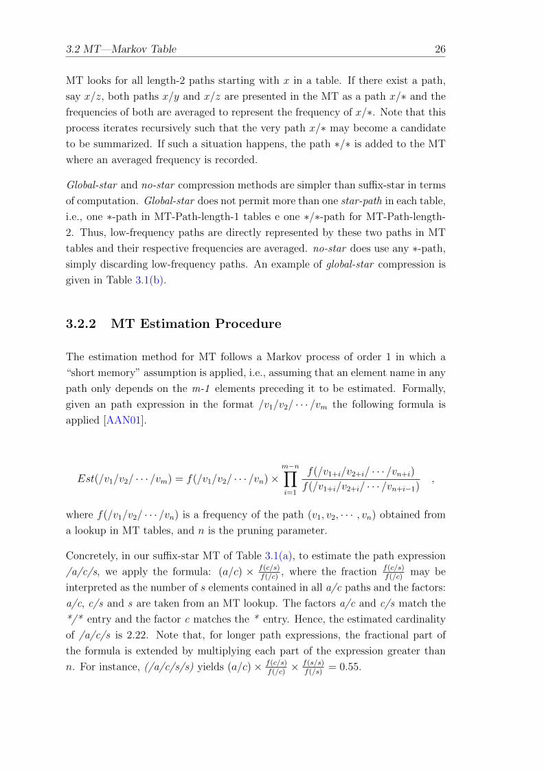
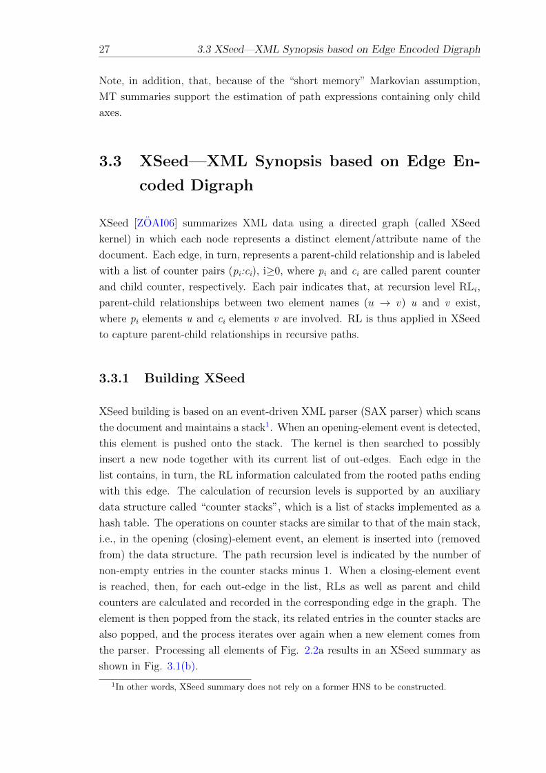
3.1 XSeed summary . . . . . . . . . . . . . . . . . . . . . . . . . . . . . 28

(a) XSeed for our recursion-free document. . . . . . . . . . . . . . 28

(b) XSeed for our recursive document. . . . . . . . . . . . . . . . 28

3.2 Situation in which XSeed breaks . . . . . . . . . . . . . . . . . . . . 29

4.1 Deriving the LESS structure. . . . . . . . . . . . . . . . . . . . . . 42

(a) HNS tree. . . . . . . . . . . . . . . . . . . . . . . . . . . . . . 42

(b) LESS structure. . . . . . . . . . . . . . . . . . . . . . . . . . . 42

4.2 LWES structure for our recursive document. . . . . . . . . . . . . . 45

(a) HNS tree. . . . . . . . . . . . . . . . . . . . . . . . . . . . . . 45

(b) LWES structure. . . . . . . . . . . . . . . . . . . . . . . . . . 45

5.1 Sketch of an ASPE node structure . . . . . . . . . . . . . . . . . . . 54

5.2 ASPE node format and EXsum summary (cut-out) . . . . . . . . . 55

(a) Format of an ASPE node for non-recursive documents. . . . . 55

(b) Partial EXsum structure. . . . . . . . . . . . . . . . . . . . . 55

5.3 Subtrees producing the same stack S configuration . . . . . . . . . 58

5.4 Configurations of EXsum and stack S (partial scan) . . . . . . . . . 59

xi

List of Figures xii

5.5 EXsum structure for our recursion-free document in Figure 2.1(c) . 62

5.6 Format of an ASPE node for recursive documents . . . . . . . . . . 63

5.7 Calculating RL for recursive paths . . . . . . . . . . . . . . . . . . . 65

5.8 EXsum state before processing the 12th element in our recursivedocument . . . . . . . . . . . . . . . . . . . . . . . . . . . . . . . . 65

5.9 EXsum state after processing the 12th element in our recursive doc-ument . . . . . . . . . . . . . . . . . . . . . . . . . . . . . . . . . . 66

5.10 EXsum for recursive paths . . . . . . . . . . . . . . . . . . . . . . . 67

5.11 Distinct path computing for a sample path stack . . . . . . . . . . . 69

5.12 EXsum extended with DPC (recursion-free document) . . . . . . . 70

5.13 EXsum extended with DPC (recursive document) . . . . . . . . . . 70

5.14 Example of an XML document with text nodes and DOM tree . . . 73

5.15 Text spoke of the p element in the example XHTML document . . . 74

5.16 Text spoke of the p element after applying some summarizationtechniques . . . . . . . . . . . . . . . . . . . . . . . . . . . . . . . . 78

6.1 Illustration of a workload processor execution. . . . . . . . . . . . . 91

6.2 Comparative accuracy: child . . . . . . . . . . . . . . . . . . . . . . 99

6.3 Comparative accuracy: descendant . . . . . . . . . . . . . . . . . . 100

6.4 Comparative accuracy: combined child+descendant steps . . . . . . 101

6.5 Comparative accuracy: parent/ancestor . . . . . . . . . . . . . . . . 102

6.6 Comparative accuracy: predicates . . . . . . . . . . . . . . . . . . . 103

6.7 Accuracy of value predicates . . . . . . . . . . . . . . . . . . . . . . 103

6.8 Accuracy of path expressions with value predicates . . . . . . . . . 104

List of Tables

3.1 MT tables (n=2, budget=4 entries) for the sample document inFigure 2.2(a). . . . . . . . . . . . . . . . . . . . . . . . . . . . . . . 25

(a) Suffix-* compression . . . . . . . . . . . . . . . . . . . . . . . 25

(b) Global-* compression . . . . . . . . . . . . . . . . . . . . . . . 25

3.2 Path-count table and Bloom histogram for our recursive document. 30

3.3 Classes to compare summary approaches . . . . . . . . . . . . . . . 33

3.4 Qualitative comparison among summary approaches . . . . . . . . . 33

4.1 Different types of histograms for a sample set of elements . . . . . . 37

(a) Set of elements . . . . . . . . . . . . . . . . . . . . . . . . . . 37

(b) Equi-width histogram . . . . . . . . . . . . . . . . . . . . . . 37

(c) Equi-height histogram . . . . . . . . . . . . . . . . . . . . . . 37

(d) End-biased histogram . . . . . . . . . . . . . . . . . . . . . . 37

(e) Biased histogram . . . . . . . . . . . . . . . . . . . . . . . . . 37

5.1 Application of estimation procedures in axis relationships. . . . . . 82

6.1 Characteristics of documents considered. . . . . . . . . . . . . . . . 90

(a) General characteristics . . . . . . . . . . . . . . . . . . . . . . 90

(b) Structural characteristics . . . . . . . . . . . . . . . . . . . . . 90

6.2 Storage size (in KBytes) . . . . . . . . . . . . . . . . . . . . . . . . 94

6.3 Memory footprint (in KBytes) . . . . . . . . . . . . . . . . . . . . . 95

6.4 Building times (in sec) . . . . . . . . . . . . . . . . . . . . . . . . . 97

6.5 Estimation times (in msec) . . . . . . . . . . . . . . . . . . . . . . . 98

6.6 NRMSE error for queries with child axes . . . . . . . . . . . . . . . 99

6.7 NRMSE error for queries with descendant axes . . . . . . . . . . . . 100

6.8 Combined NRMSE error for queries with child and descendantsteps (in %) . . . . . . . . . . . . . . . . . . . . . . . . . . . . . . . 101

6.9 NRMSE error for queries with parent and ancestor steps . . . . . . 101

6.10 NRMSE error for queries with predicates . . . . . . . . . . . . . . . 102

xiii

List of Algorithms

4.1 Building a LESS structure . . . . . . . . . . . . . . . . . . . . . . . . 41

4.2 Building a LWES structure . . . . . . . . . . . . . . . . . . . . . . . 46

5.1 Handles the occurrence of a element name when parsing the document 57

5.2 Processes a new path to be added to EXsum structure . . . . . . . . 60

5.3 ComputeDPC. Computes the distinct paths for child and descen-

dant spokes . . . . . . . . . . . . . . . . . . . . . . . . . . . . . . . . 68

xiv

Abbreviations

ASPE Axes Summary Per Element

BH Bloom Histogram

DPC Distinct Path Count

EB End-Biased histogram

EB-MVBD End-Biased histogram with Min.Var. Bucket Descriptor

EH Equi-Height histogram

EW Equi-Width histogram

EXsum Element-centered XML Summarization

HNS Hierarchical Node Summarization

LESS Leaf-Element-in-Subtree Summarization

LWES Level-Wide Element Summarization

MOSEL Multiple Occurrences of the Same Element name in a Level

MT Markov Table

PS Path Synopsis

PT Path Tree

RL Recursion Level

XSeed XML Synopsis based on Edge Encoded Digraph

xv

Chapter 1

Introduction

There is nothing more difficult to take in hand, more perilous to conduct, or more uncertain in

its success, than to take the lead in the introduction of a new order of things.

Niccolo Machiavelli, Italian writer and statesman, 1469 – 1527. In: The Prince.

1.1 The Advent of XML and Semi-Structured

Data

Since the early ages of computer science, particularly in the information systems

area, scientists and practitioners struggle with data models. A data model is a

representation of real-world entities based on a particular view. Hence, an abstrac-

tion of the real world is provided by a data model and as abstraction only the most

relevant aspects of the real-world entities are considered. The other non-relevant

aspects of the world (under the data model’s point of view) are not considered.

For instance, the Entity-Relationship Model sees the world as a set of entities,

with their attributes and the relationships among entities.

Data models allow the user to (easily) manage of the complexity of a knowledge

domain, enable the comprehension of the domain and further provide a base for

applications to be developed. In addition, and most importantly, they provide a

description of the data which is called, generically, metadata or schema.

The degree of detail in a data model can be used to classify it into a conceptual

data model, which represents the world with no concern as to how this represen-

tation should be materialized. Logical data models are more directed to the data

1

1.1 The Advent of XML and Semi-Structured Data 2

materialization. For example, the Entity-Relationship Model can be considered

conceptual. Physical data models play a key role in databases and, in general,

in data management systems. We can cite three well-known logical data models

which have been used for years in databases.

The Hierarchical Model (HM) [LHH00, JKM+02] only recognizes record type, as

a representation of a world entity, and 1-to-n record type relationships. The

CODASYL-DBTG (or networked) Model [TF76, Oll78], in turn, is more flexible

to permit n-to-m relationships among record types.

The Relational Model (RM) [Cod83, Cod90] sees the world entities as relations

— a tabular structure, table, for short, compound of columns representing the

attributes of entities. Several relationships among tables can be represented in

RM, e.g., 1-to-1, 1-to-n, and n-to-m.

A common characteristic of these data models is that they require a database

designer to store the schema first, and all (raw) data instances coming after must

strictly adopt the metadata provided. It means that, when an evolution (modifi-

cation) in the data structure is necessary, the schema must be modified and data

instances unloaded and then reloaded with the new schema. Therefore, these data

models are considered structured. In the structured data models, it is not possible

to have, in the database, a data instance which does not completely satisfy the

schema (metadata).

Structured data models present true advantages. The schema information may be

used for typical database tasks such as transaction processing and query process-

ing. For example, the data type information in the schema may be used for query

parse and optimization tasks. The relationships among entities represented may

be useful as synchronization information in concurrency control providing a kind

of meta-synchronization.

The actual high demand for information in several application areas such as enter-

prise systems integration, the World Wide Web, data streams and mobile environ-

ments, has led to a need for a more flexible data model in which it is permissible

for some data instances residing in a database to not strictly obey the schema. In

other words, the schema should not be a barrier but a driver for data storage and

manipulation. This is the so-called semi-structured data model that has the XML

(eXtensible Markup Language) as its representative exponent.

3 1.1 The Advent of XML and Semi-Structured Data

1.1.1 XML—A Brief History

In the 1970’s, a group of researchers (Charles Goldfarb — considered the “father”

of XML, Ed Mosher, and Ray Lorie) working at IBM invented the GML, a way

to mark up technical documents with structural tags. GML stands for Goldfarb-

Mosher-Lorie, and this acronym was given specifically to highlight the markup

capability. Later on, GML became SGML (Standard Generalized Markup Lan-

guage) and, in the late 1980’s, it had presented benefits for dynamic information

display as realized by digital media publishers. SGML was added to W3C (The

World Wide Web Consortium) in 1995 by Dan Connolly.

The first sub-product of the SGML — as a simplification of it and, in fact, a

SGML application, has been HTML (Hyper-Text Markup Language) that has been

applied to render content pages — whether to the World Wide Web (WWW) or to

digital documents. However, HTML has suffered a lack of a discipline as software

companies (e.g., Microsoft and Netscape) have created their own dialects of the

original HTML proposal.

SGML being too complex, and HML not suitable for structured data, in the late

1990’s, a group of people including Jon Bosak, Tim Bray, James Clark, and others

came up with XML, or eXtensible Markup Language, which is also a sub-set of

SGML, meant to be readable by people via semantic constraints; application lan-

guages can be implemented in XML. The W3C immediately set about reshaping

HTML as an XML application, with the result being XHTML. The first XML

working draft was released by the W3C in November, 1997 and a W3C recom-

mendation for XML — called XML 1.0, in February, 1998.

The key point is that using XML the industry can specify how to store almost

any kind of data, in a form that applications running on any platform can easily

import and process1.

1.1.2 XML-related Technologies

The XML technology has produced several related products and specifications, all

of them managed by the W3C. Here, we indicate some of them.

1We cannot state, though, that XML is “self-describing” in the sense that it is understandablefor any hardware/software platform. Under the database point of view, however, XML bringstogether, in a mixed way, value and structure interleaving them in a unit called XML document.

1.1 The Advent of XML and Semi-Structured Data 4

• XML Namespaces enable the same document to contain XML elements

and attributes taken from different vocabularies, without any naming colli-

sions occurring.

• XInclude defines the ability for XML files to include all or part of an ex-

ternal file.

• XML Signature defines the syntax and processing rules for creating digital

signatures on XML content.

• XML Encryption defines the syntax and processing rules for encrypting

XML content.

• XPointer is a system for addressing components of XML-based Internet

media.

• XSLT is a declarative, XML-based document transformation language.

Under the database technology point of view, two XML-related products have had

a profound impact in the database industry, whether for researchers or practition-

ers: XPath and XQuery.

• XPath makes it possible to refer to individual parts of an XML document.

XPath expressions can refer to all or part of the text, data, and values in

XML documents.

• XQuery is to XML and XML databases what SQL is to relational databases:

ways to access, manipulate, and return XML. In fact, XQuery uses XPath

as its sub-language.

1.1.3 The XML Document

The unit in which the XML specification is materialized is called XML document

(or document, for short). In the structure of an XML document, we find two

kinds of construct: element and attribute. Elements are disposed in a hierarchical

(nested) way and have names. Hence, the order of the elements2 matters in a

document. They are represented by start-tags (<>) and end-tags (</>). For

instance, an element called Kaiserslautern is represented by <Kaiserslautern>...

</Kaiserslautern>. Attributes are a set of name-value pairs annotated in an

2Also called document order. Accordingly, the internal structure of an XML document iscommonly referred to as document tree.

5 1.1 The Advent of XML and Semi-Structured Data

element start-tag. For instance, if Kaiserslautern has two attributes called zip

and abbrev, it is represented as <Kaiserslautern zip=67655, abbrev=KL>... </

Kaiserslautern>. Attributes in an attribute list are separated by comma and the

order is irrelevant among attributes.

An XML document has two levels of correctness, in ascending order of correctness:

Well-formed and Valid.

1. Well-formed. A well-formed document conforms to the XML syntax rules;

i.e., each start-tag must appear with a corresponding end-tag. This is

the minimum correctness criteria provided for XML. A document not well-

formed is not an XML document. This means that it is not accepted to be

processed.

2. Valid. A valid document conforms additionally to semantic rules, defined

by the user through an XML Schema or DTD (Document Type Definition).

XML Schema and DTD may be considered as metadata of XML, because they

describe an XML document. The difference is that XML Schema yields more

expressiveness than DTD, allowing data type definition in addition to the struc-

ture. However, XML Schema and DTD cannot be taken in the same meaning as

a database metadata. Being semi-structured data, an XML document can vary in

its level of correctness, permitting tags in the document to be different than the

specification. For example, one can start to make a valid document regarding to

a specific schema and later on, insert some tag into it which was not defined origi-

nally in the schema, thus downgrading the correctness level of the document. It is

worthwhile to note that, different from relational databases, this is not considered

a schema violation, rather a common characteristic of XML and of semi-structured

data in general.

If only a well-formed document is required, XML is a generic framework for storing

any amount of text or any data whose structure can be represented as a tree. The

only indispensable syntactical requirement is that the document has exactly one

root element (also known as the document element or document root), i.e. the

entire document must be enclosed between a root start-tag and a corresponding

root end-tag.

Under each tag, as leaf nodes of a document tree, it may contain data values.

Theoretically, any data type can be nested under a tag. For example, if a university

is called TU Kaiserslautern, we can represent it as <university>TU Kaiserslautern

1.1 The Advent of XML and Semi-Structured Data 6

</university>. Here, the (text) value “TU Kaiserslautern” is the value part under

university.

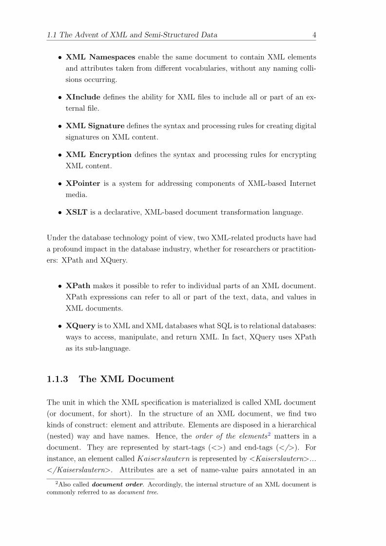
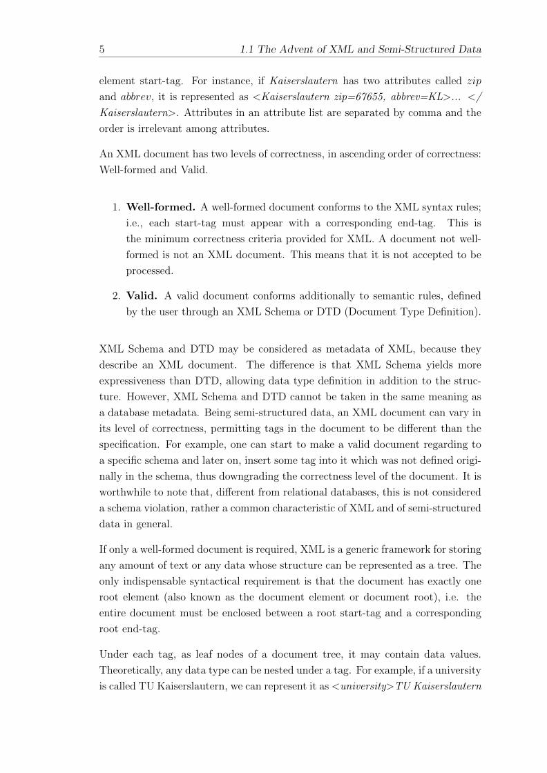
In summary, an XML document tree is compounded by document nodes which can

represent a tag, attribute (structural part) or a value. A sample XML document

together with its graphical tree representation is given in figures 1.1(a) and 1.1(b),

respectively.

<regions> % The document root <Rheinland-Pfalz> % an element <Kaiserslautern zip=67655, abbrev=KL> % an element with attributes <university> TU Kaiserslautern % a value </university> </Kaiserslautern> <Mainz zip=55116> % another element <fh> FH Mainz </fh> </Mainz> <Trier abbrev=TR> </Trier> </Rheinland-Pfalz></regions>

(a) Human intelligible.

regions

Rheinland-Pfalz

Kaiserslautern Mainz Trier

zip abbrev zip abbrevuniversity

67655 KL 55116 TRTU Kaiserslautern

fh

FH Maiz

elementvalue

attribute

Document Node Types

(b) Document tree.

Figure 1.1: An XML document in both representations

1.1.4 Processing XML Documents

An XML document may be stored as a plain file in a file system of any operating

system as well as in a database management system (DBMS) in native mode, i.e.,

keeping the native tree structure; or in shredded mode, i.e., mapping the document

to another underlying structure (e.g., relational tables and columns).

In addition to typical database processing techniques, there are three ways to

process an XML document using a programming language.

• SAX (Simple API for XML), an API in which the processing is made on

a tag-at-a-time basis without the need to load the entire document into

memory.

• DOM (Document Object Model), an API in which the document is first

entirely loaded into memory and then processed.

• A transformation language such as XSLT.

7 1.2 XML Data Management

While the transformation way can be built on top of SAX or DOM, these two ways

have advantages and disadvantages. SAX normally requires less memory space

than DOM to process a document. However, SAX processing is limited to only

one-way direction. In SAX, when an element/attribute is processed, there is no

way to return to it. In contrast, DOM can navigate throughout the document, in

both forward (root-to-leave) direction and reverse (leave-to-root) direction. DOM

will require, however, a memory space proportional to the document size which

may not be suitable in many practical situations. SAX processing, in turn, gets

the same memory space regardless of the document size.

1.2 XML Data Management

Both shredded and native database processing of XML documents also have ad-

vantages and disadvantages. For shredding processing, a relational database en-

gine is normally used. In this case, a document is mapped to (a set of) tables and

columns, thus breaking its native structure. For instance, a row may contain a doc-

ument node and each column can store information regarding the document node

(e.g., element/attribute name and/or value). Using a relational engine, one can

benefit from proven features of the relational database management systems such

as transaction management and query processing and reuse them. An additional

software layer should be provided to enable document mapping and unmapping.

This layer should provoke a non-negligible burden because, as the XML document

is broken (shredded) to enable its use in a relational storage, it must be recon-

structed as a result of a query. Nevertheless, a shredded document is processed as

relational data, not taking into account the specific needs and idiosyncrasies of a

native XML data management. Instead the processing unit being a document, it

is a table. A document query in a shredded scenario is made with SQL language

or SQL/XML, an extension of SQL enabling specific document operations and (a

limited form of) XPath/XQuery expressions.

Pure XML data management systems (XDBMS), in turn, store an XML docu-

ment, keeping its entire tree structure. Normally, B-trees are used as supporting

structure to hold the document order 3. In XDBMS, the document is the process-

ing unit and tailored techniques for transaction and query processing are designed.

An XDBMS uses XPath and/or XQuery for querying stored documents. Query

results are also XML documents which are sent back to the user with no need

for remapping. XDBMS tailors transaction techniques to support a multi-user

3The document node ordering generated by a depth-first traversal of the document tree

1.2 XML Data Management 8

processing of a document and also query processing techniques to support the

particularities of XQuery and XPath languages.

Over the last few years, hybrid data engines with the capability of storing natively

both relational tables and XML documents have appeared in the database market.

The most recent versions of the IBM DB2, Oracle’s Oracle and Microsoft SQL

Server bring this capability.

Nevertheless, in any case, all database engines have a common requirement, which

is the method of uniquely identifying a document node. Note that, different from

relational databases in which a tuple ID identifies a tuple in the database, for XML

document nodes a node ID has to be devised and this node ID is independent from

the element/attribute name. This means that two elements with the same name

have mandatorily different node IDs.

1.2.1 Identifying Document Nodes

Identifying document nodes for shredded and native storage is accomplished by a

Labeling Method. Whatever the labeling method is, the basic idea is to assign a

unique numbering system to each document node assuring the document order.

There are several labeling methods published in literature that we can classify into

two categories: range-based and prefix-based labeling.

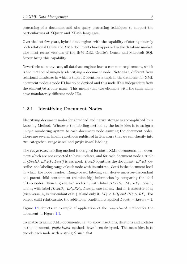
The range-based labeling method is designed for static XML documents, i.e., docu-

ment which are not expected to have updates, and for each document node a triple

of (DocID, LP:RP, Level) is assigned. DocID identifies the document; LP:RP de-

scribes the labeling range of each node with its subtree. Level is the document level

in which the node resides. Range-based labeling can derive ancestor-descendant

and parent-child containment (relationship) information by comparing the label

of two nodes. Hence, given two nodes n1 with label (DocID1, LP1:RP1, Level1)

and n2 with label (DocID2, LP2:RP2, Level2), one can say that n1 is ancestor of n2

(vice-versa, n2 is descendant of n1), if and only if, LP1 < LP2 and RP1 > RP2. For

parent-child relationship, the additional condition is applied Level1 = Level2 − 1.

Figure 1.2 depicts an example of application of the range-based method for the

document in Figure 1.1.

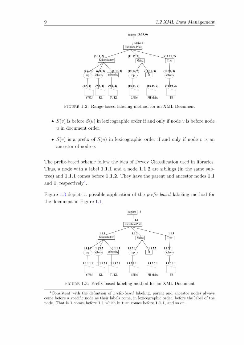
To enable dynamic XML documents, i.e., to allow insertions, deletions and updates

in the document, prefix-based methods have been designed. The main idea is to

encode each node with a string S such that,

9 1.2 XML Data Management

regions

Rheinland-Pfalz

Kaiserslautern Mainz Trier

zip abbrev zip abbrevuniversity

67655 KL 55116 TRTU KL

fh

FH Mainz

(1:23, 0)

(2:22, 1)

(3:11, 2) (11:17, 2) (17:21, 2)

(4:6, 3)

(5:5, 4)

(6:8, 3)

(7:7, 4) (9:9, 4)

(8:10, 3) (12:14, 3) (14:16, 3)

(13:13, 4) (15:15, 4)

(18:20, 3)

(19:19, 4)

Figure 1.2: Range-based labeling method for an XML Document

• S(v) is before S(u) in lexicographic order if and only if node v is before node

u in document order.

• S(v) is a prefix of S(u) in lexicographic order if and only if node v is an

ancestor of node u.

The prefix-based scheme follow the idea of Dewey Classification used in libraries.

Thus, a node with a label 1.1.1 and a node 1.1.2 are siblings (in the same sub-

tree) and 1.1.1 comes before 1.1.2. They have the parent and ancestor nodes 1.1

and 1, respectively4.

Figure 1.3 depicts a possible application of the prefix-based labeling method for

the document in Figure 1.1.

regions

Rheinland-Pfalz

Kaiserslautern Mainz Trier

zip abbrev zip abbrevuniversity

67655 KL 55116 TRTU KL

fh

FH Mainz

1

1.1

1.1.1 1.1.2 1.1.3

1.1.1.1

1.1.1.1.1

1.1.1.2

1.1.1.2.1 1.1.1.3.1

1.1.1.3 1.1.2.1 1.1.2.2

1.1.2.1.1 1.1.2.2.1

1.1.3.1

1.1.3.1.1

Figure 1.3: Prefix-based labeling method for an XML Document

4Consistent with the definition of prefix-based labeling, parent and ancestor nodes alwayscome before a specific node as their labels come, in lexicographic order, before the label of thenode. That is 1 comes before 1.1 which in turn comes before 1.1.1, and so on.

1.2 XML Data Management 10

Both methods, range-based and prefix-based labeling, maintain the document or-

der and easily derive the computation of parent/ancestor nodes. Range-based

methods, however, do not yield immutable labels when updates come, provoking a

relabeling in such cases. Prefix-based labeling, on the other hand, guarantees that

a label is immutable for the lifetime of the nodes. Nevertheless, both methods

support declarative query processing with XQuery/XPath languages.

1.2.2 Querying XML Documents

Since declarative query languages (XQuery/XPath) for XML documents have been

proposed and recommended by the W3C, the database community has now to

face the challenge of how to derive appropriate query engines to effectively process

XPath/XQuery queries.

Some best practices learned from relational databases have to be applied and

adapted for querying XML documents. For example, the derivation of an algebraic

representation of the query expression, the optimization (algebraic and/or cost-

based) of the query execution plans (QEP), and the physical operators.

XML algebras have been proposed, such as XAT (XML Algebra Tree) [ZPR02],

TAX (Tree Algebra for XML) [JLST02], NAL [MHM03] and NAL-STJ [Mat07],

and others [SA02, NZ06]. None, though, have qualified to become a standard XML

algebra, leaving an open issue of how to find a suitable algebraic representation

for XML queries5.

Several physical operators (also called Path Processing Operators, or PPO) have

appeared. Structural Join (STJ) [AKJP+02, WPJ03, MHH06] was the first pro-

posal and processes a query by a set of joins. Each join corresponds to a part of

the query expression. The Twig Join family [LCL04, BLS07] evaluates a query

by building a query pattern (twig) and finds matches in the document to this

twig. Holistic Twig Join (HTJ) [BKS02] was an improvement on the idea of tree-

pattern matching in which the twig is evaluated as a whole, without any partial

pattern match. Some variations of HTJ exist, for example, Index Twig Join (ITJ)

[JWLY03], Optimal Twig(O-HTJ) [FJSY05], and HTJ for OR-predicates [JLW04].

In any case, there is already room for new operators to be proposed6.

5XQuery has been verified to be a Turing-complete language [Kep04]. Such finding compli-cates the design of an appropriated algebraic representation of XQuery even more.

6HTJ has produced a plethora of HTJ-based algorithms, normally focusing on a specific issueof HTJ. We have omitted these here and refer only the main algorithms of the HTJ family.

11 1.2 XML Data Management

While STJ has a simple execution model — inherited from relational the nested-

loop join operator, and lends itself to be modeled as a (simple) cost formula;

Twig join algorithms, specially HTJ, are hard to model. This means that a cost

model for enabling cost-based XML query processing is still a long way off, there

is a plethora of opportunities to develop a proposal. However, one empirical cost

model has already been proposed in [WH09].

Whatever the cost model adopted, statistics on documents are fundamental in

order to derive, as accurately as possible, node cardinality/selectivity factors to

enable appropriated cost-based decisions on which QEP should be considered the

best plan. XML document statistics are normally gathered in a (generic) struc-

ture called summary. An XML summary congregates, in a condensed form, all

document node cardinalities along with their relationships to provide estimations

of query expressions or even parts of the expressions. The representation of an

XML summary is based on element/attribute (node) names rather than node IDs.

1.2.3 Motivation for this Work

Over the past ten years, several proposals of XML summaries [GW97, AAN01,

FHR+02, LWP+02, PG02, PG06, WJLY04, ZOAI06] have appeared in the liter-

ature. Regarding the degree of a summary’s document coverage, approaches can

be classified into two categories: Structural summaries and Content-and-Structure

(CAS) summaries.

Structural summaries [GW97, AAN01, FHR+02, LWP+02, WJLY04, ZOAI06]

summarize only the structural part of a document, not considering the (text) value

distributions. CAS summaries [PG02, PG06] try to condense both structural and

value distributions modeling dependencies between value and structure. The ma-

jority of publications focus on a statistical coverage of structural relationships

among document nodes. In addition, some works [AAN01, FHR+02, WJLY04]

apply compression techniques (e.g., histograms [Ioa03]) to the summary structure.

Collecting document statistics implies maintenance tasks for them. Summary

updates have to take place when the document is changed by a user application to

preserve the close correspondence of document and related statistics. This aspect,

however, is hardly addressed in XML summary proposals. Only [LWP+02] and

[WJLY04] claim to provide some solution. Most proposals assume (explicitly or

tacitly) off-line summary update by re-scanning the entire document periodically.

1.3 Thesis Overview 12

A methodical weakness of many publications is the insufficient basis of experimen-

tal data. Frequently, they only rely on a few documents, often very small and/or

with synthetic data. Furthermore, they do not provide any clues on their use with

a query optimizer. Except for quality estimation results, important items such as:

• the space needed to store the summary,

• the necessary memory footprint to be used in the estimation process, and

• how fast the access to the summary is — so as to not impact query opti-

mization time

are normally not presented in the publications.

1.3 Thesis Overview

This thesis tackles the hard problem of summarizing an XML document. This

problem is so difficult due mainly to the mixed nature of an XML document

which encompass varying distributions in its structural part and in its value part.

Furthermore, the structural recursion allowed (and sometimes frequently) in a

document complicates the summarization process.

1.3.1 Our Contributions

Trying to overcome the drawbacks of published XML summary works, and as the

main contribution of this thesis, we have proposed three new XML summary struc-

tures called: LESS (Leaf-Element-in-Subtree Summary), LWES (Level-Wide El-

ement Summarization) [AMFH08a, AMFH08c], and EXsum (Element-centered

XML summarization) [AMFH08b]. The former two are basically structural sum-

maries, whereas the latter is a CAS summary.

LESS and LWES follow the “conventional” method of summarizing documents

in the sense that they mirror somewhat the document structure. EXsum, in

turn, puts aside the strict document order structure and inaugurates a new way

to summarize XML documents.

Furthermore, we have made the following contributions.

13 1.3 Thesis Overview

• We have created an extension to the End-Biased histogram [IP95] called EB-

MVBD which makes suitable the use of histograms in the XML estimation

process, and applied EB-MVBD to compress LESS and any other structure

that needs such a feature.

• We have made the application of histograms in XML summaries flexible,

so that the application is tailored according to a specific query workload

[AMFH08c].

• For the cases, in which histogram application is not profitable, we have

proposed a (simple) bit-list compression method.

• We have designed estimation procedures and/or heuristics for all proposed

summaries.

A (hopefully extensive) set of experiments is also included with a set of documents

of varying characteristics and sizes to stress and cross-compare our approaches with

the competing ones. For that,

• we have constructed a Query Workload Generator tool which generates sev-

eral types of XPath queries. This tool can be extended to generate XQuery

queries.

• Additionally, a Query Workload Processor has been implemented which ex-

ecutes the query workload against the XTC XDBMS.

The analysis of the empirical results has been directed by the effective summary use

for the query optimizer. Therefore, we have elicited three criteria which impact the

optimization process and have evaluated all summaries (proposed and competing

ones) under these criteria.

• Sizing. Further divided into the following sub-criteria.

– Storage Space needed to persist the summary structure in the XDBMS7.

– Memory footprint required by the summary to estimate queries.

• Timing. Further divided into the following sub-criteria.

7Note that, because all summaries have been implemented into our XDBMS (see Chapter 6),we have used its Metadata Component. The Storage Space criterion, however, takes only netsize of the structure into account, thus disregarding the specific information overhead of theMetadata’s underlying structure.

1.3 Thesis Overview 14

– Building Time is the time needed to construct the summary which

includes the time for the document scan — done normally through a

SAX parser, and running the respective building algorithm.

– Estimation Time is the time necessary to estimate queries.

• Estimation Quality translated quantitatively into an error metric in which

the lower error is, the higher the estimation quality provided.

1.3.2 Structure

This thesis is structured as follows. In Chapter 2, we present all necessary termi-

nology, basic concepts and definitions which will be used throughout the thesis.

Chapter 3 studies the existing XML summary approaches and, at the end, makes

a qualitative discussion and comparison. Chapters 4 and 5 introduce our XML

summary proposals. For each proposed summary, we detail its general idea, the

building algorithms, and the estimation procedures. The empirical study comes in

the Chapter 6. The set of document considered are presented, the query workload

is detailed, and the analysis based on the aforementioned criteria is performed.

This thesis is concluded in Chapter 7 in which, additionally, some future research

directions are pointed out.

Chapter 2

Preliminaries: Terminology, Basic

Concepts, and Definitions

The words printed here are concepts. You must go through the experiences.

Saint Augustine, African Bishop of Hippo Regius, Doctor of the Church, 354 – 430

2.1 Overview

This chapter introduces the definitions and concepts that will be used through-

out the thesis. Section 2.2 defines terms used throughout the remainder of this

document. Some references to well-known XML documents – e.g., dblp, nasa, and

treebank, are made in this chapter and in Section 6.2.1 we show in detail their

physical characteristics (in tables 6.1(a) and 6.1(b)). Section 2.3 exhibits the ba-

sic definitions of XML summarization. We give, in Section 2.4, the details on what

should be considered as the most trivial XML summary, called HNS. Section 2.5

concludes this chapter. Figures 2.1(a), 2.1(c) and 2.2(a) depict sample documents

which will be used as running examples throughout this thesis.

2.2 Terminology

When speaking of XML summaries, we should define terms clearly in order to

keep from provoke a misunderstanding. We call a summary node simply a node.

When referring to nodes in an XML document, we use the expression “document

15

2.2 Terminology 16

a

c tc u

sr

ts ps p s p t u

r r s s s

p p s u

tt t

(a) A very Regular Document.

a

c t u

s p t u

r s

p u s

t

p

(b) The corresponding PS.

t p

ss

spt t

p p p u u

p

u

a

cc

t

p p p p

p s s

p p

s sp

pp p

(c) A Document with some structural variability.

a

tc p

t s sp

u

pp s

t

p(d) The corresponding PS.

Figure 2.1: Recursion-free XML documents and their respective Path Syn-opses

t p

ss

spt t

p p p u u

p

u

a

cc

t

p p p p

p s s

p p

s sp

pp p

st s

pp p

s

p

s

t(a) Recursive document.

a

tc p

t s

s

s

p

t

p

u

p

s

s

p

p

t

p

s

t

p

(b) The corresponding PS.

Figure 2.2: Recursive XML document and path synopsis

17 2.2 Terminology

node”. General references to a document node name, i.e., a set of document nodes

with the same name, are termed element names. Accordingly, attribute name

is used generically to refer to document attribute names.

2.2.1 Terms in XML Query Languages

Path expressions are the base for declarative XML languages. In fact, XPath and

XQuery use them as a sub-language. Therefore, it is necessary to define terms

used when referring to path expressions.

Definition 2.1. Path expression: A path expression is a set of location steps (also

called path steps or steps, for short) and, optionally, predicates.

Definition 2.2. Location Step (Step): A location step is a compound of the

following three items, in this order:

1. Context Node: the context under which the node test should be verified. In

most cases, it is implicitly determined.

2. Axis : One of the possible axes in the XML document. For example, child

(/), parent (parent ::), ancestor (ancestor::), descendant (descendant::), self

(.), descendant-or-self (//), following sibling (following-sibling::), preceding

sibling (preceding-sibling::) and so on. We can further classify axes as:

• Forward axis: it follows the document nodes in a top-down fashion,

i.e., root-to-node way. Child (/), descendant (descendant::), self (.),

descendant-or-self (//) and following sibling (following-sibling::) are

examples of forward axes.

• Reverse axis: it follows the document nodes in a bottom-up fashion,

i.e., node-to-root way. Parent (parent::), ancestor (ancestor::) and pre-

ceding sibling (preceding-sibling::) are examples of reverse axes.

3. Node test : A reference to a document node name to be verified under a pair

context/axis.

More intuitively, a path expression has a format: /v1/v2/ . . . /vn, where vi are

node tests, /’s represent axes and context nodes are as follows: document root

for the step /v1, v1 for the step /v2, · · · , and /vn−1 for the last step /vn. As a

concrete example drawn from our sample document (see Figure 2.1(c)), we may

have /a/c/t representing the retrieval of all document nodes whose name is t that

are children (/) of c nodes which are in turn children of a.

2.2 Terminology 18

It is worthwhile to note the declarative characteristic of path expressions. A path

expression says what should be retrieved, but not how it is to be retrieved. They

state, in addition, restrictions (or order), represented by the axes, to retrieve nodes.

A more complex example is //p/parent :: s/ancestor :: c getting all nodes c which

are ancestors of s as parents of all sub-trees rooted by a document node p1.

Definition 2.3. Predicates : A predicate is an expression enclosed into brackets ([

]) occurring in any place in a path expression. Predicates can be further classify

into

• Existential Predicates, which allow only path expressions inside the brackets.

For example, //c/t[./s].

• Value Predicates which check for value contents. For example //c/t[text() =′

XML′].

Predicates can use AND/OR logical connectors. For example, //c/t[./text() =′

XML′ or contains(.,′ document′)]. Note also that functions as defined in [W3C07]

may take place. Predicates place a filter on the result. In this example, we want

to retrieve t nodes being children of every subtree rooted by c that additionally

have either the vale “XML” or contain a string called “document” under them.

The variability of path expressions and predicates involved may be so rich that

a single auxiliary structure (as complex as conceivable) for an XML summary

would not solve all query estimation/optimization problems. Moreover, the more

sophisticated a summary is, the more maintenance overhead would be needed.

Hence, a practical XML summary is necessarily confined in its scope, but should

be expressive enough to capture the most important structural properties of XML

data and flexible enough to deliver, as accurate as possible, the most frequently

requested cardinality estimates for cost-based XQuery/XPath query optimization.

We are aware that some path expressions—including their predicates, if they

exist—can be rewritten linguistically or algebraically2. Nevertheless, on purpose

of gathering statistics and the estimation process, we should provide support, as

widely as possible, to estimate them. However, we do not claim that our propos-

als cover all possible path expressions. To the contrary, we are focused on the

most important kinds of path expressions. Therefore, we make an observation

that child and descendant axes are considered first-class citizens, and parent and

1In other words, retrieving all nodes c having a descendant s as a parent of every sub-treerooted by p.

2For example, rewriting path expressions to favor forward axes and then to try to “standard-ize” the expression in the first tasks of query processing.

19 2.3 Basic Concepts

ancestor axes deserve a second-class citizenship. The other axes are considered

less important for all practical situations.

In any case, we need to define some basic concepts before we dive into details of

the approaches.

2.3 Basic Concepts

In XML documents, as illustrated by our sample documents, many path instances

only differ from each other in the leaf values, and in the order they occur in the

documents. Therefore, their structural part can be represented by a single unique

path, called path class. Taking advantage of this observation, DataGuides [GW97]

was the first approach to XML summarization aimed at providing a structural

overview for the user and a data structure for storing statistical document in-

formation, thus enabling the query optimization. Later proposals, called path

synopses (PS), are similar to DataGuides, but are used as a query (document)

guide and a compact structure view in the first place (see figures 2.1(b), 2.1(d)

and 2.2(b)). Other applications are possible for a PS. For example, document

structure virtualization, concurrency control, and support of indexing and query

processing [HMS07, SH07, BHH09]. This synopsis has to be complemented with a

summarization structure for statistical information concerning elements and axis

relationships [AMFH08b, AMFH08a].

A cyclic-free XML schema captures all information needed for the path synopsis;

otherwise, this data structure can be constructed while the document (sent by

a client) is stored in the database. Typical path synopses have only a limited

number of element names and path classes and can, therefore, be represented

in a small memory-resident data structure. As shown in the following, such a

concise description of the document structure is a prerequisite for effective query

optimization.

Definition 2.4. Path Class : A representation of all path instances of the docu-

ment having the same sequence of element names.

Definition 2.5. Path Synopsis : A tree structure capturing all path classes existing

in a document.

Definition 2.6. Unique Element Name: An element name that occurs only once

in the path synopsis.

2.3 Basic Concepts 20

Definition 2.7. Homonyms : Element names occurring more than once in the

path synopsis, but not in the same path class.

Definition 2.8. Recursive Path: Occurs when element names appear more than

once in a single path class.

An unique element name such as a, c, or u in our sample path synopses results in an

unambiguous summarization, which makes path expression estimation very simple

in some cases. In turn, a homonym-free document has only unique element names

in its path synopsis, and it is non-recursive by definition, but may be an exception.

In the typical case, a document containing a varying degree of homonyms may have

most (or even all) of its paths without any level of recursion, i.e., homonyms do

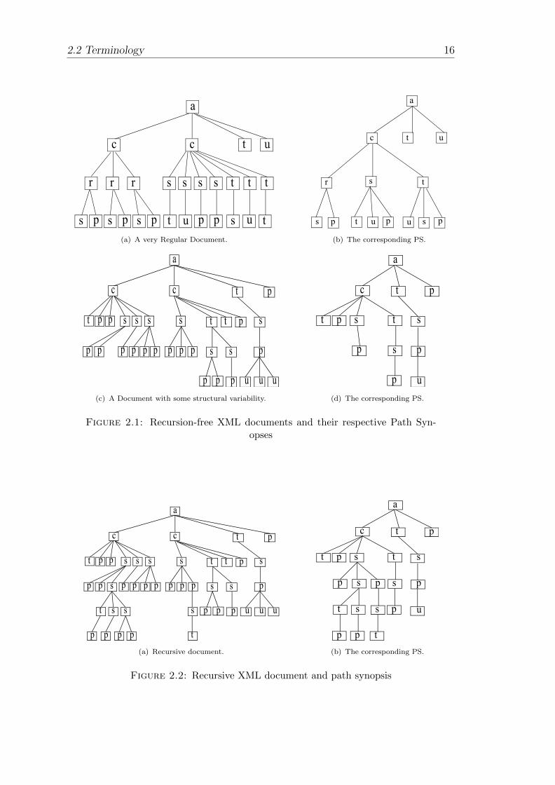
not occur in the same path class3 (see Figure 2.1).

In contrast, we have to deal with recursion in a document as soon as an element

name occurs more than once in a single path class, e.g., in paths (a,c,s,s,s,p) or

(a,c,s,p,s,t) (see Figure 2.2). Highly recursive XML documents such as treebank

(see Table 6.1(a)) are exotic outliers and not frequent in practice; therefore, they

do not deserve first-class citizenship. However, some degree of recursion may be

anticipated in a small class of documents. Thus, we analyze recursiveness for rea-

sons of generality and evaluate summarization structures that support documents

exhibiting a (limited) kind of structural recursion, too.

The concept of recursion level (RL) was introduced in [ZOAI06] as a way to better

represent structural recursion in XML documents and explained the case where

only a single element name could recur in a path. Recursion levels were defined

as follows.

Definition 2.9. Recursion Level (RL): Given a rooted path in the XML tree, the

maximum number of occurrences of any label (element name) minus 1 is the path

recursion level (PRL). The recursion level of a node in the XML tree is defined to

be the PRL of the path from root to this node.

Thus, given path (a,c,s,s,t), the second s node has RL=1 and all other nodes have

RL=0, whereas the PRL of this path is 1.

3dblp has 41 element names where 32 are homonyms resulting in 146 nodes for the pathsynopsis. Hence, the avg. repetition of a homonym is more than 4. The numbers for elementnames, homonyms, and path synopsis nodes are (100, 6, 264) and (70, 12, 111) for swissprot andnasa, respectively. Because nasa has only a share of 6% homonyms, the estimation procedureshould be particularly simple and accurate. In all cases, the data structure for the path synopsisremains very small.

21 2.4 HNS—Hierarchical Node Summarization

Recursion can also occur in query expressions, making the estimation even more

difficult (and, often, more imprecise). For recursive path expressions, we follow

the definition in [ZOAI06].

Definition 2.10. Recursive Path Expression: A path expression is recursive with

respect to an XML document if an element in the document could be matched by

more than one node test in the expression.

Thus, it is easy to see that path expressions only consisting of /-axes (or parent

axes) are not recursive. However, //s//s is a recursive path expression on the

XML tree in Figure2.2a, because a recursively occurring s node could be matched

by both node tests. Hence, recursive path expressions always involve at least one

//-axis (or ancestor axis) and are usually applied to recursive documents.

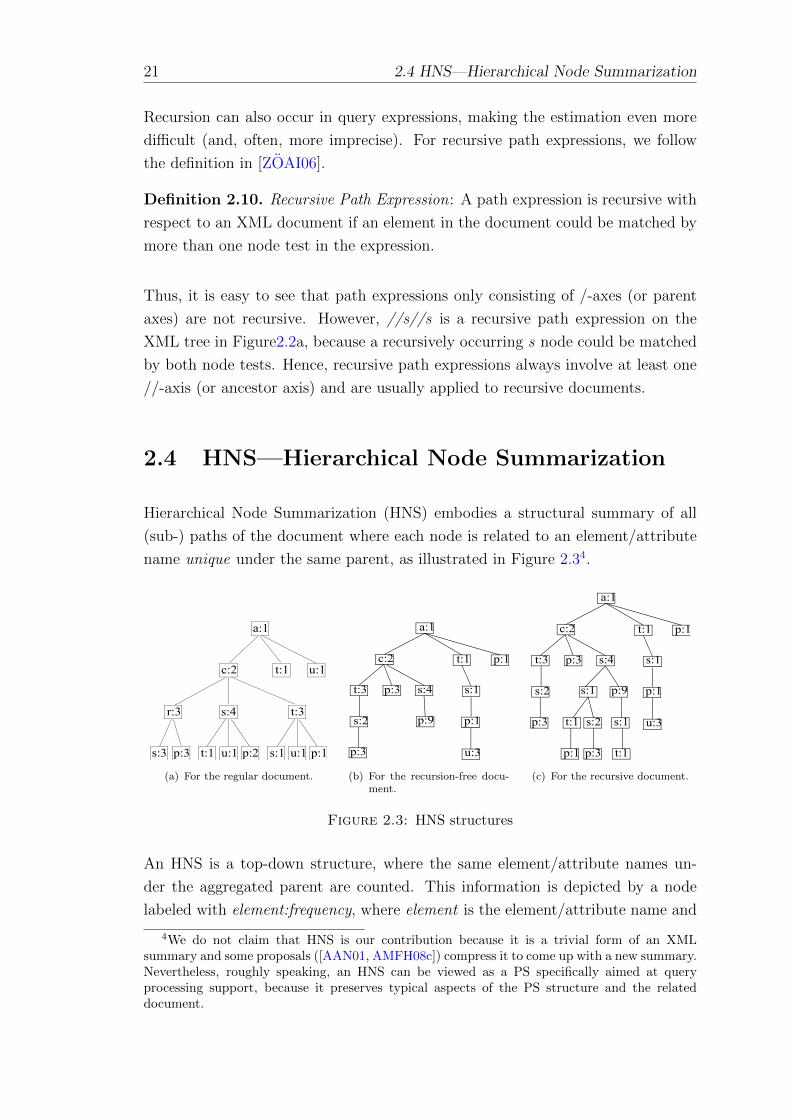
2.4 HNS—Hierarchical Node Summarization

Hierarchical Node Summarization (HNS) embodies a structural summary of all

(sub-) paths of the document where each node is related to an element/attribute

name unique under the same parent, as illustrated in Figure 2.34.

a:1

c:2 t:1 u:1

s:3 p:3 t:1 u:1

r:3 s:4

p:2 s:1 u:1

t:3

p:1

(a) For the regular document.

a:1

t:1c:2 p:1

p:9

t:3 s:4

s:2

s:1

p:3

p:3

u:3

p:1

(b) For the recursion-free docu-ment.

a:1

t:1c:2 p:1

p:9

t:3 s:4

s:2

s:1

p:3

p:3

u:3

p:1s:1

s:1s:2t:1

p:1 p:3 t:1

(c) For the recursive document.

Figure 2.3: HNS structures

An HNS is a top-down structure, where the same element/attribute names un-

der the aggregated parent are counted. This information is depicted by a node

labeled with element:frequency, where element is the element/attribute name and

4We do not claim that HNS is our contribution because it is a trivial form of an XMLsummary and some proposals ([AAN01, AMFH08c]) compress it to come up with a new summary.Nevertheless, roughly speaking, an HNS can be viewed as a PS specifically aimed at queryprocessing support, because it preserves typical aspects of the PS structure and the relateddocument.

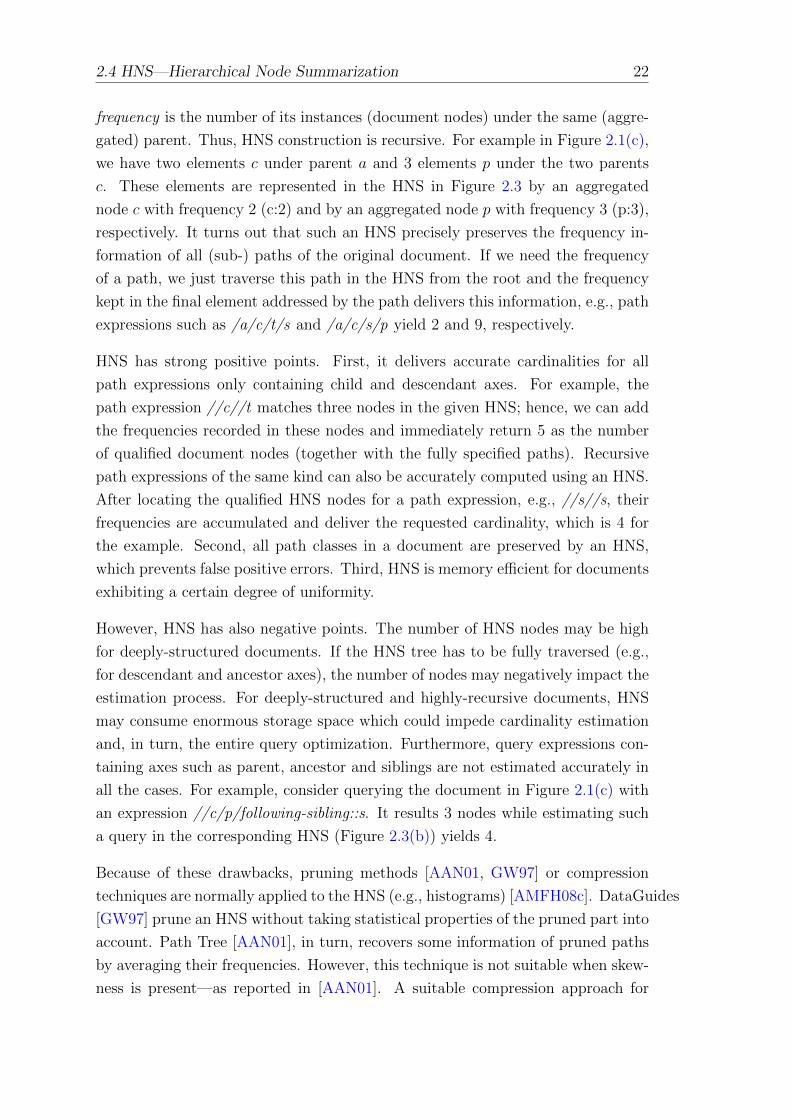
2.4 HNS—Hierarchical Node Summarization 22

frequency is the number of its instances (document nodes) under the same (aggre-

gated) parent. Thus, HNS construction is recursive. For example in Figure 2.1(c),

we have two elements c under parent a and 3 elements p under the two parents

c. These elements are represented in the HNS in Figure 2.3 by an aggregated

node c with frequency 2 (c:2) and by an aggregated node p with frequency 3 (p:3),

respectively. It turns out that such an HNS precisely preserves the frequency in-

formation of all (sub-) paths of the original document. If we need the frequency

of a path, we just traverse this path in the HNS from the root and the frequency

kept in the final element addressed by the path delivers this information, e.g., path

expressions such as /a/c/t/s and /a/c/s/p yield 2 and 9, respectively.

HNS has strong positive points. First, it delivers accurate cardinalities for all

path expressions only containing child and descendant axes. For example, the

path expression //c//t matches three nodes in the given HNS; hence, we can add

the frequencies recorded in these nodes and immediately return 5 as the number

of qualified document nodes (together with the fully specified paths). Recursive

path expressions of the same kind can also be accurately computed using an HNS.

After locating the qualified HNS nodes for a path expression, e.g., //s//s, their

frequencies are accumulated and deliver the requested cardinality, which is 4 for

the example. Second, all path classes in a document are preserved by an HNS,

which prevents false positive errors. Third, HNS is memory efficient for documents

exhibiting a certain degree of uniformity.

However, HNS has also negative points. The number of HNS nodes may be high

for deeply-structured documents. If the HNS tree has to be fully traversed (e.g.,

for descendant and ancestor axes), the number of nodes may negatively impact the

estimation process. For deeply-structured and highly-recursive documents, HNS

may consume enormous storage space which could impede cardinality estimation

and, in turn, the entire query optimization. Furthermore, query expressions con-

taining axes such as parent, ancestor and siblings are not estimated accurately in

all the cases. For example, consider querying the document in Figure 2.1(c) with

an expression //c/p/following-sibling::s. It results 3 nodes while estimating such

a query in the corresponding HNS (Figure 2.3(b)) yields 4.

Because of these drawbacks, pruning methods [AAN01, GW97] or compression

techniques are normally applied to the HNS (e.g., histograms) [AMFH08c]. DataGuides

[GW97] prune an HNS without taking statistical properties of the pruned part into

account. Path Tree [AAN01], in turn, recovers some information of pruned paths

by averaging their frequencies. However, this technique is not suitable when skew-

ness is present—as reported in [AAN01]. A suitable compression approach for

23 2.5 Conclusion

an HNS tree is called Level-Wide Element Summarization (LWES) [AMFH08c],

which captures the element distributions per tree level by applying histograms.

2.5 Conclusion

The concepts introduced in this chapter form a necessary background for the

discussions in the following chapters. Furthermore, we have introduced a trivial

kind of summary structure called HNS. HNS has served as a base structure to

come up with several other summaries published in the literature — including two

of our proposals.

However, before we introduce our proposals in Chapter 4 and Chapter 5, we review

the existing summaries in the literature and then make a qualitative discussion of

each of them in the next chapter.

Chapter 3

Existing Summarization Methods

Study the past if you would define the future.

K’ung fu-tsu (Confucius), Chinese philosopher, 551 BC – 479 BC. In: Anaclets.

3.1 Overview

In this chapter, we present a non-exhaustive list of summarization approaches

published in literature. We detail each work in its respective section describing the

main idea, building process, and estimation procedures (Section 3.2 to Section 3.4).

For each class of our qualitative comparison (and discussion), in Section 3.5, we

have chosen one representative summary and study each one.

3.2 MT—Markov Table

Markov Table [AAN01] is a structural summary which is built by mapping docu-

ment paths together with their frequencies into two-column tables. One column

represents the document paths of a specified length, whereas the second column

provides the frequencies of the corresponding paths. Note that document paths

may be retrieved from an HNS (see Section 2.4).

Markov Tables (MT) compress the HNS by pruning paths up to length n, where n

is a parameter set by the user. The pruned part is approximated by the application

of both: a Markov model and some statistical information on a generic path called

star-path—indicated in [AAN01] by ∗ or ∗/∗. In other words, if n = 2, MT

24

25 3.2 MT—Markov Table

prunes (deletes) low-frequency paths of lengths 1 and 2 and discards also paths

with lengths >2. Based on pruning and star-path, MT provides three compression

techniques: suffix-star, global-star and no-star. The latter technique does not

apply a star-path, but just relies on pruning.

3.2.1 Building and Compressing MT

Building MT is driven by two parameters: the pruning parameter n and a memory

budget. The latter can be translated into a maximum size in bytes of the entire

MT structure or in a maximum number of entries in MT. The former specifies the

number of tables to be created. For example, for n = 2, there will be two tables,

one with paths of length=1 and another with paths of length=2.

MT building proceeds in such way that, for n = 2, all paths of length 1 will

be in the MT-Path-Length-1 table and all paths of length 2 will be in the MT-

Path-Length-2 table. For example, in MT-Path-Length-1 table, we have entries:

(/a:1 ), (/c:2 ), (/t:4 ), (/s:7 ) and so on. For MT-Path-Length-2 table, we have:

(/a/c:2 ), (/a/t:1 ), and so on. Note that MT-Path-Length-1 table corresponds to

the number of occurrences of each distinct element name in the document. At this

point, because the memory budget is normally exceeded, compression techniques

take place. In general, these compression methods recursively delete entries in MT

tables substituting them with star-paths, until the memory budget is reached.

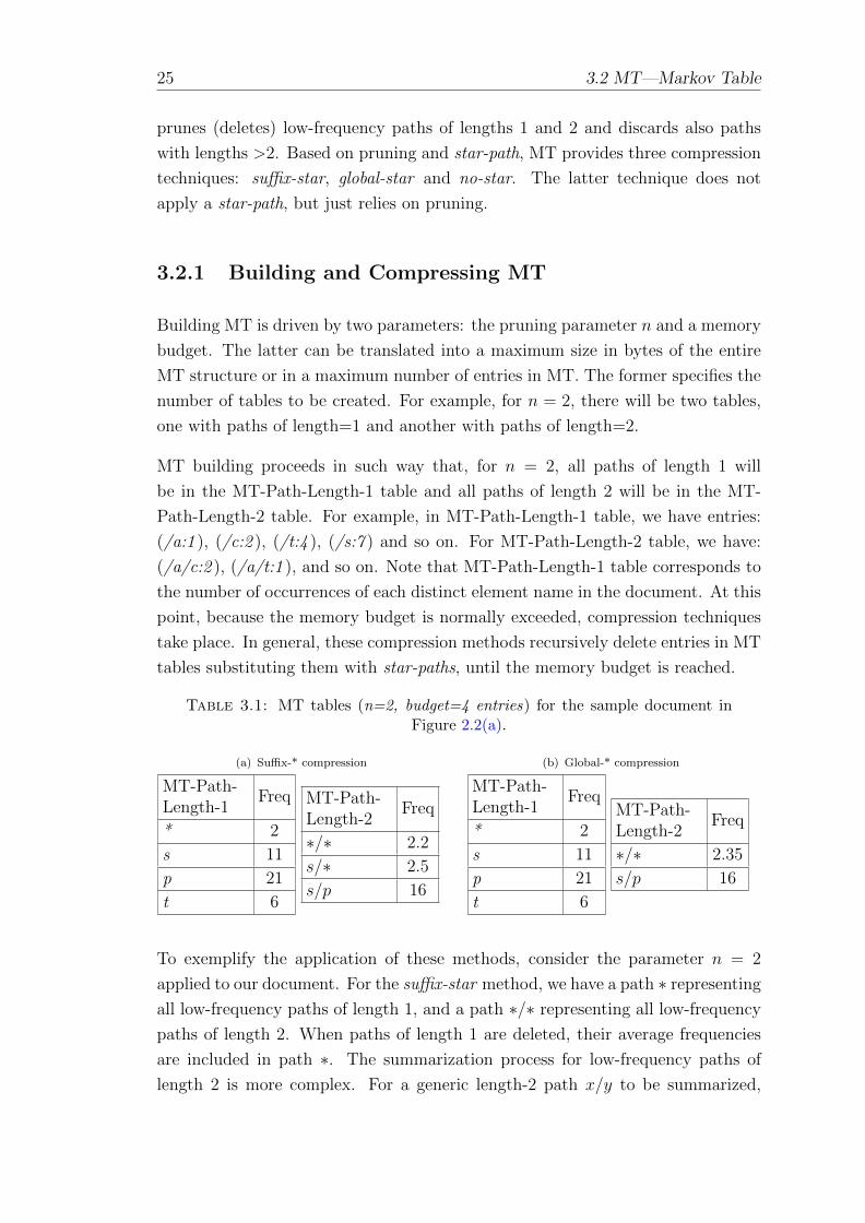
Table 3.1: MT tables (n=2, budget=4 entries) for the sample document inFigure 2.2(a).

(a) Suffix-* compression

MT-Path-Length-1

Freq

* 2

s 11

p 21

t 6

MT-Path-Length-2

Freq

∗/∗ 2.2

s/∗ 2.5

s/p 16

(b) Global-* compression

MT-Path-Length-1

Freq

* 2

s 11

p 21

t 6

MT-Path-Length-2

Freq

∗/∗ 2.35

s/p 16

To exemplify the application of these methods, consider the parameter n = 2

applied to our document. For the suffix-star method, we have a path ∗ representing

all low-frequency paths of length 1, and a path ∗/∗ representing all low-frequency

paths of length 2. When paths of length 1 are deleted, their average frequencies

are included in path ∗. The summarization process for low-frequency paths of

length 2 is more complex. For a generic length-2 path x/y to be summarized,

3.2 MT—Markov Table 26

MT looks for all length-2 paths starting with x in a table. If there exist a path,

say x/z, both paths x/y and x/z are presented in the MT as a path x/∗ and the

frequencies of both are averaged to represent the frequency of x/∗. Note that this

process iterates recursively such that the very path x/∗ may become a candidate

to be summarized. If such a situation happens, the path ∗/∗ is added to the MT

where an averaged frequency is recorded.

Global-star and no-star compression methods are simpler than suffix-star in terms

of computation. Global-star does not permit more than one star-path in each table,

i.e., one ∗-path in MT-Path-length-1 tables e one ∗/∗-path for MT-Path-length-

2. Thus, low-frequency paths are directly represented by these two paths in MT

tables and their respective frequencies are averaged. no-star does use any ∗-path,

simply discarding low-frequency paths. An example of global-star compression is

given in Table 3.1(b).

3.2.2 MT Estimation Procedure

The estimation method for MT follows a Markov process of order 1 in which a

“short memory” assumption is applied, i.e., assuming that an element name in any

path only depends on the m-1 elements preceding it to be estimated. Formally,

given an path expression in the format /v1/v2/ · · · /vm the following formula is

applied [AAN01].

Est(/v1/v2/ · · · /vm) = f(/v1/v2/ · · · /vn)×m−n∏i=1

f(/v1+i/v2+i/ · · · /vn+i)

f(/v1+i/v2+i/ · · · /vn+i−1),

where f(/v1/v2/ · · · /vn) is a frequency of the path (v1, v2, · · · , vn) obtained from

a lookup in MT tables, and n is the pruning parameter.

Concretely, in our suffix-star MT of Table 3.1(a), to estimate the path expression

/a/c/s, we apply the formula: (a/c) × f(c/s)f(/c)

, where the fraction f(c/s)f(/c)

may be

interpreted as the number of s elements contained in all a/c paths and the factors:

a/c, c/s and s are taken from an MT lookup. The factors a/c and c/s match the

*/* entry and the factor c matches the * entry. Hence, the estimated cardinality

of /a/c/s is 2.22. Note that, for longer path expressions, the fractional part of

the formula is extended by multiplying each part of the expression greater than

n. For instance, (/a/c/s/s) yields (a/c)× f(c/s)f(/c)

× f(s/s)f(/s)

= 0.55.

27 3.3 XSeed—XML Synopsis based on Edge Encoded Digraph

Note, in addition, that, because of the “short memory” Markovian assumption,

MT summaries support the estimation of path expressions containing only child

axes.

3.3 XSeed—XML Synopsis based on Edge En-

coded Digraph

XSeed [ZOAI06] summarizes XML data using a directed graph (called XSeed

kernel) in which each node represents a distinct element/attribute name of the

document. Each edge, in turn, represents a parent-child relationship and is labeled

with a list of counter pairs (pi:ci), i≥0, where pi and ci are called parent counter

and child counter, respectively. Each pair indicates that, at recursion level RLi ,

parent-child relationships between two element names (u → v) u and v exist,

where pi elements u and ci elements v are involved. RL is thus applied in XSeed

to capture parent-child relationships in recursive paths.

3.3.1 Building XSeed

XSeed building is based on an event-driven XML parser (SAX parser) which scans

the document and maintains a stack1. When an opening-element event is detected,

this element is pushed onto the stack. The kernel is then searched to possibly

insert a new node together with its current list of out-edges. Each edge in the

list contains, in turn, the RL information calculated from the rooted paths ending

with this edge. The calculation of recursion levels is supported by an auxiliary

data structure called “counter stacks”, which is a list of stacks implemented as a

hash table. The operations on counter stacks are similar to that of the main stack,

i.e., in the opening (closing)-element event, an element is inserted into (removed

from) the data structure. The path recursion level is indicated by the number of

non-empty entries in the counter stacks minus 1. When a closing-element event

is reached, then, for each out-edge in the list, RLs as well as parent and child

counters are calculated and recorded in the corresponding edge in the graph. The

element is then popped from the stack, its related entries in the counter stacks are

also popped, and the process iterates over again when a new element comes from

the parser. Processing all elements of Fig. 2.2a results in an XSeed summary as

shown in Fig. 3.1(b).

1In other words, XSeed summary does not rely on a former HNS to be constructed.

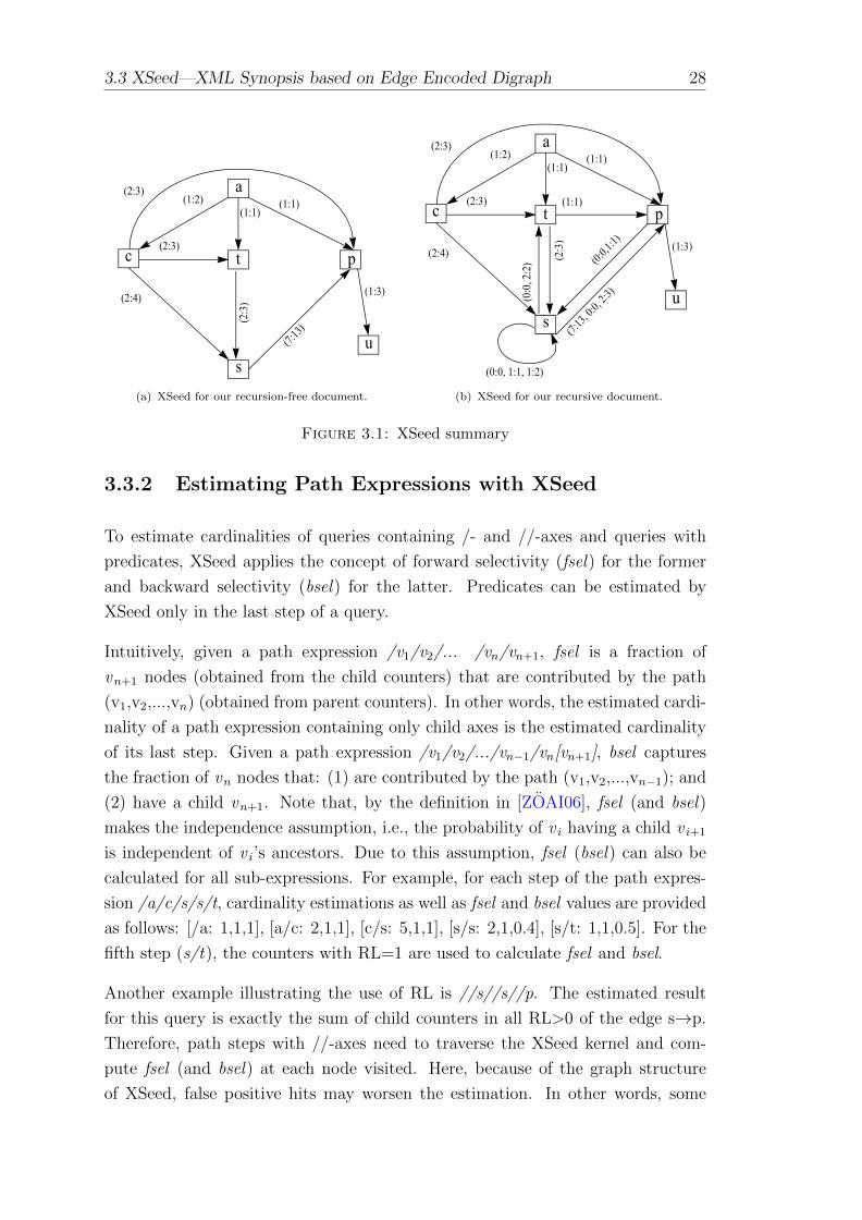
3.3 XSeed—XML Synopsis based on Edge Encoded Digraph 28

a

tc p

su

(1:2)(1:1)

(1:3)(2:4)

(7:13)

(2:3)

(2:3)(2:3)

(1:1)

(a) XSeed for our recursion-free document.

a

tc p

su

(1:2)(1:1)

(1:3)(2:4)

(0:0, 1:1, 1:2)

(0:0

, 2:2

)

(7:13,

0:0, 2:

3)

(2:3)

(2:3)

(2:3

)

(1:1)

(1:1)

(0:0,1

:1)

(b) XSeed for our recursive document.

Figure 3.1: XSeed summary

3.3.2 Estimating Path Expressions with XSeed

To estimate cardinalities of queries containing /- and //-axes and queries with

predicates, XSeed applies the concept of forward selectivity (fsel) for the former

and backward selectivity (bsel) for the latter. Predicates can be estimated by

XSeed only in the last step of a query.

Intuitively, given a path expression /v1/v2/... /vn/vn+1, fsel is a fraction of

vn+1 nodes (obtained from the child counters) that are contributed by the path

(v1,v2,...,vn) (obtained from parent counters). In other words, the estimated cardi-

nality of a path expression containing only child axes is the estimated cardinality

of its last step. Given a path expression /v1/v2/.../vn−1/vn[vn+1], bsel captures

the fraction of vn nodes that: (1) are contributed by the path (v1,v2,...,vn−1); and

(2) have a child vn+1. Note that, by the definition in [ZOAI06], fsel (and bsel)

makes the independence assumption, i.e., the probability of v i having a child v i+1

is independent of v i’s ancestors. Due to this assumption, fsel (bsel) can also be

calculated for all sub-expressions. For example, for each step of the path expres-

sion /a/c/s/s/t, cardinality estimations as well as fsel and bsel values are provided

as follows: [/a: 1,1,1], [a/c: 2,1,1], [c/s: 5,1,1], [s/s: 2,1,0.4], [s/t: 1,1,0.5]. For the

fifth step (s/t), the counters with RL=1 are used to calculate fsel and bsel.

Another example illustrating the use of RL is //s//s//p. The estimated result

for this query is exactly the sum of child counters in all RL>0 of the edge s→p.

Therefore, path steps with //-axes need to traverse the XSeed kernel and com-

pute fsel (and bsel) at each node visited. Here, because of the graph structure

of XSeed, false positive hits may worsen the estimation. In other words, some

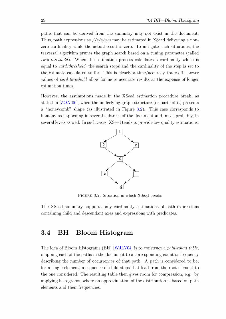
29 3.4 BH—Bloom Histogram

paths that can be derived from the summary may not exist in the document.

Thus, path expressions as //s/s/s/s may be estimated in XSeed delivering a non-

zero cardinality while the actual result is zero. To mitigate such situations, the

traversal algorithm prunes the graph search based on a tuning parameter (called

card threshold). When the estimation process calculates a cardinality which is

equal to card threshold, the search stops and the cardinality of the step is set to

the estimate calculated so far. This is clearly a time/accuracy trade-off. Lower

values of card threshold allow for more accurate results at the expense of longer

estimation times.

However, the assumptions made in the XSeed estimation procedure break, as

stated in [ZOAI06], when the underlying graph structure (or parts of it) presents

a “honeycomb” shape (as illustrated in Figure 3.2). This case corresponds to

homonyms happening in several subtrees of the document and, most probably, in

several levels as well. In such cases, XSeed tends to provide low quality estimations.

a

e

b c

d

f

g

Figure 3.2: Situation in which XSeed breaks

The XSeed summary supports only cardinality estimations of path expressions

containing child and descendant axes and expressions with predicates.

3.4 BH—Bloom Histogram

The idea of Bloom Histograms (BH) [WJLY04] is to construct a path-count table,

mapping each of the paths in the document to a corresponding count or frequency

describing the number of occurrences of that path. A path is considered to be,

for a single element, a sequence of child steps that lead from the root element to

the one considered. The resulting table then gives room for compression, e.g., by

applying histograms, where an approximation of the distribution is based on path

elements and their frequencies.

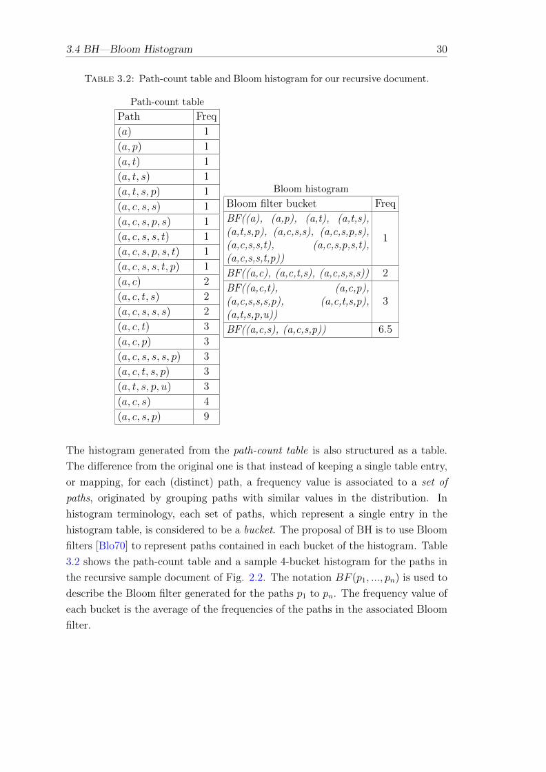
3.4 BH—Bloom Histogram 30

Table 3.2: Path-count table and Bloom histogram for our recursive document.

Path-count table

Path Freq

(a) 1

(a, p) 1

(a, t) 1

(a, t, s) 1

(a, t, s, p) 1

(a, c, s, s) 1

(a, c, s, p, s) 1

(a, c, s, s, t) 1

(a, c, s, p, s, t) 1

(a, c, s, s, t, p) 1

(a, c) 2

(a, c, t, s) 2

(a, c, s, s, s) 2

(a, c, t) 3

(a, c, p) 3

(a, c, s, s, s, p) 3

(a, c, t, s, p) 3

(a, t, s, p, u) 3

(a, c, s) 4

(a, c, s, p) 9

Bloom histogram

Bloom filter bucket Freq

BF((a), (a,p), (a,t), (a,t,s),(a,t,s,p), (a,c,s,s), (a,c,s,p,s),(a,c,s,s,t), (a,c,s,p,s,t),(a,c,s,s,t,p))

1

BF((a,c), (a,c,t,s), (a,c,s,s,s)) 2

BF((a,c,t), (a,c,p),(a,c,s,s,s,p), (a,c,t,s,p),(a,t,s,p,u))

3

BF((a,c,s), (a,c,s,p)) 6.5

The histogram generated from the path-count table is also structured as a table.

The difference from the original one is that instead of keeping a single table entry,

or mapping, for each (distinct) path, a frequency value is associated to a set of

paths, originated by grouping paths with similar values in the distribution. In

histogram terminology, each set of paths, which represent a single entry in the

histogram table, is considered to be a bucket. The proposal of BH is to use Bloom

filters [Blo70] to represent paths contained in each bucket of the histogram. Table

3.2 shows the path-count table and a sample 4-bucket histogram for the paths in

the recursive sample document of Fig. 2.2. The notation BF (p1, ..., pn) is used to

describe the Bloom filter generated for the paths p1 to pn. The frequency value of

each bucket is the average of the frequencies of the paths in the associated Bloom

filter.

31 3.4 BH—Bloom Histogram

3.4.1 Constructing BH

BH building is a two-phase process. In the first phase, the path-count table is to

be constructed. It can be done by traversing an HNS structure, if it exists, or

scanning the entire document. Whatever the method used, the path-count table

needs to be sorted on its frequency column (see column “Freq” in Table 3.2). This

process has a time complexity of O(nlogn), where n is the number of table entries2.

The second phase is to compress the path-count table by using a histogram. The

histogram construction technique proposed by BH uses a dynamic programming

algorithm which has a time complexity of O(n2b), where n is the number of path-

count table entries and b is the number of buckets chosen3. The histogram ap-

plication obtains the correct number of histogram buckets boundaries (with the

least error in each bucket) to be used according to a desired error metric. After

constructing the histogram, Bloom filters are applied in the set of paths in each

bucket and the building process of BH is finished.

3.4.2 BH Estimation Procedure

BH inherits the probabilistic nature of the Bloom filter. Consequently, some ratio

of false positives are allowed and this ratio is directly related to the parameters

used for the Bloom filter4.

In other words, some buckets can report True for a path containment test/

verification even if the path is not present in the bucket. To overcome such sit-

uations, the BH estimation procedure always returns the average of bucket fre-

quencies, if more than one bucket signalize True in a histogram table lookup.

Therefore, to estimate a path expression, BH needs always to scan the entire BH

table and test the bloom filter at each bucket. Additionally, the augment of the

number of buckets in BH does not provoke an increase in estimation quality, rather,

it is possible to lead to a lower quality.

In summary, the user has to control and make trade-offs between the number of

buckets and the sizes of Bloom filters in order to adjust BH to produce quality

2The number of path-count table entries is exactly the number of distinct paths in a document,i.e., the number of path classes in PS (or HNS). As an example, dblp, nasa, swissprot and treebankdocuments have 136, 161, 264, and 338,749 path classes, respectively.

3Because of this quadratic mechanism and, in addition, the sort needed for the first phase,the BH building time may become, in some cases, prohibitive.

4Basically, the number of bits, the error ratio allowed, and the number of hash functions used.

3.5 Discussion and Qualitative Comparison 32

estimations. Another restriction to the BH structure is related to the support of

path expressions, which is limited to path expressions with only child axes.

3.5 Discussion and Qualitative Comparison

After having studied the most important summaries published, it is necessary to

have a discussion, comparing them qualitatively. To accomplish this, we must first

find some classification criterion as well as some comparison criteria.

3.5.1 Classification

For this propose, we separate the existing approaches into two different classes:

probabilistic methods and non-probabilistic approaches which we further refine

based on their structural characteristics, i.e., their shapes: tree-based, graph-

based and table-based. Hence, MT and BH are classified as non-probabilistic/

table-based and probabilistic/table-based, respectively. XSeed is classified into

non-probabilistic/graph-based and Path Tree (PT) [AAN01] is a non-probabilistic/

tree-based approach (see Table 3.3)5. A probabilistic classification is considered if

a summary structure, by its own virtue, allows false-positive and/or false-negative

hits. The opposite case is the non-probabilistic methods.

As an example, we have classified MT as non-probabilistic, although MT uses a

Markovian model to estimate expressions. However, the MT structure does not

allow false positive/negative hits. XSeed, on the other hand, allows inexistent

paths to be derived from its structure, i.e., the structure can evaluate path expres-

sions that have an empty result as a non-empty expression result. This is clearly

a false-positive hit. Therefore, we have classified XSeed as a probabilistic method.

3.5.2 Comparison

Table 3.4 summarizes and compares the characteristics of the summary approaches

discussed so far in a qualitative way. The criteria compared are scalability, esti-

mation, loading, pruning, and support for path axes.

5Aboulnaga et al. [AAN01] have proposed both PT and MT. The only difference betweenthem is: the format – PT is tree-structured and MT is table-structured – and the estimationprocedure – PT estimates based on a tree traversal and MT estimates based on a Markovianassumption. However, PT and MT rely on similar compression techniques. We have referred toPT here for sake of completeness of our qualitative comparison.

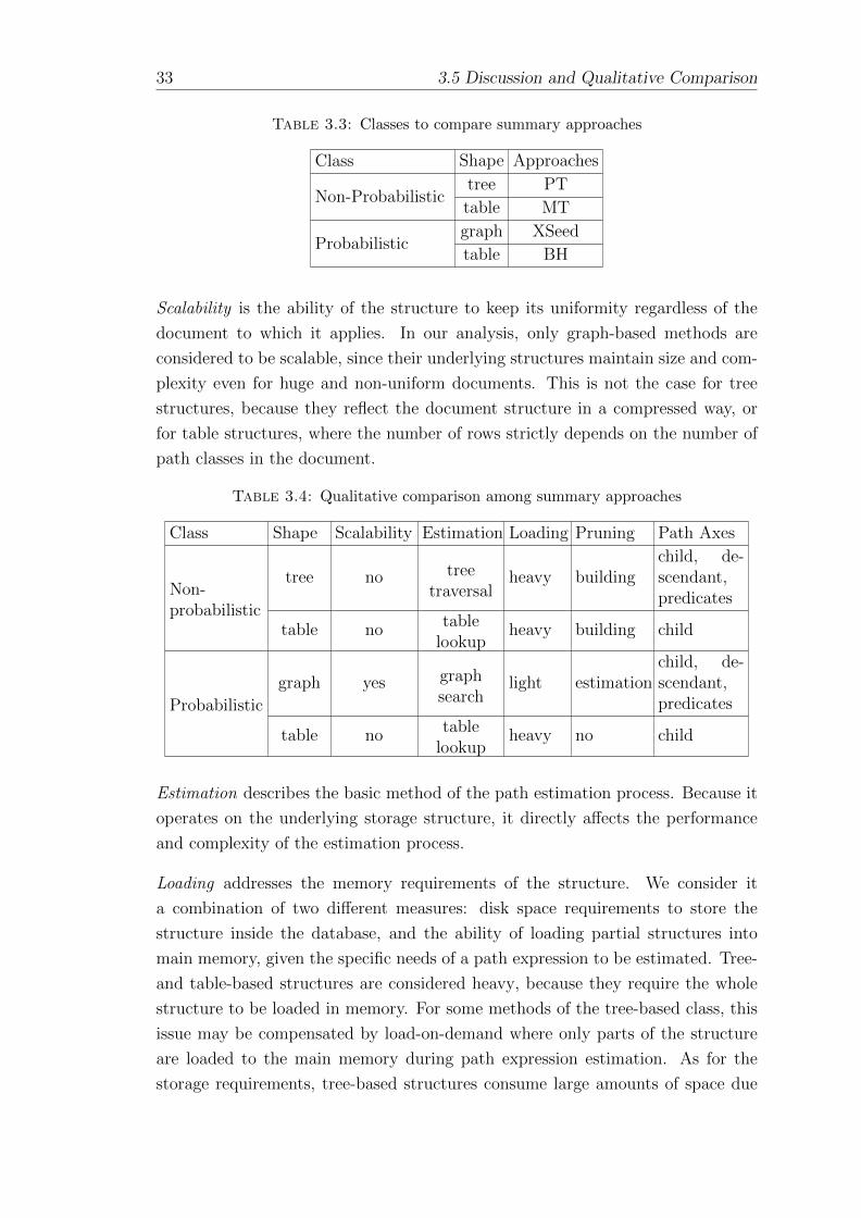
33 3.5 Discussion and Qualitative Comparison

Table 3.3: Classes to compare summary approaches

Class Shape Approaches

Non-Probabilistictree PT

table MT

Probabilisticgraph XSeed

table BH

Scalability is the ability of the structure to keep its uniformity regardless of the

document to which it applies. In our analysis, only graph-based methods are

considered to be scalable, since their underlying structures maintain size and com-

plexity even for huge and non-uniform documents. This is not the case for tree

structures, because they reflect the document structure in a compressed way, or

for table structures, where the number of rows strictly depends on the number of

path classes in the document.

Table 3.4: Qualitative comparison among summary approaches

Class Shape Scalability Estimation Loading Pruning Path Axes

Non-probabilistic

tree no treetraversal

heavy buildingchild, de-scendant,predicates

table notable

lookupheavy building child

Probabilistic

graph yes graphsearch

light estimationchild, de-scendant,predicates

table notable

lookupheavy no child

Estimation describes the basic method of the path estimation process. Because it

operates on the underlying storage structure, it directly affects the performance

and complexity of the estimation process.

Loading addresses the memory requirements of the structure. We consider it

a combination of two different measures: disk space requirements to store the

structure inside the database, and the ability of loading partial structures into

main memory, given the specific needs of a path expression to be estimated. Tree-

and table-based structures are considered heavy, because they require the whole

structure to be loaded in memory. For some methods of the tree-based class, this

issue may be compensated by load-on-demand where only parts of the structure

are loaded to the main memory during path expression estimation. As for the

storage requirements, tree-based structures consume large amounts of space due

3.5 Discussion and Qualitative Comparison 34

to the fact that they preserve the tree structure of the document. This is not the

case for tables, but, because of their bad scalability, we cannot generally assume

low space requirement. Graph structures, on the other hand, have a light load, as

they are scalable and have a high degree of compression. However, the graph-based

class does not allow load on demand.

Pruning a summary structure can be performed during structure building and

cardinality estimation. Pruning in the building phase consists of setting bound-

aries for the document navigation and is usually done by specifying a maximal

number of (upper) levels up to which the structure keeps the accurate numbers of

occurrences, while for lower levels only guesses can be derived for them from the

summary (normally, based on a statistical model). For tree-based structures, this

corresponds to a standard tree pruning, where the summary has the same limita-

tions concerning the number of levels as those used for the document navigation.

Pruning can also be applied to table building, where the sizes of the paths stored

are restricted by the given level boundary. The second type of pruning applies to

the estimation process and, in our analysis, only to graph-based structures. The

technique aims to set a limit to graph navigation, thereby avoiding unacceptable

estimation times, however, at the expense of estimation accuracy. In the XSeed

study made in Section 3.3, this is done by the “card threshold” parameter which

controls the trade-off between estimation time and accuracy.

For the flexibility, expressiveness, and usefulness of a summary class for cardinality

estimation and, in turn, query optimization, support of path axes is decisive. Our

rating in Table 3.4 records the path axes supported for cardinality estimation of

path steps and whether a summary enables selectivity estimation for predicates6.

Note, however, that some approaches are so restrictive in the use of path axes

(e.g., table-based) and even if their underlying structures would allow estimation

of specific axes, they do not provide such a support. As a matter of fact, most

of the evaluated methods only deliver cardinality estimations for (/) and (//)

axes. Estimation techniques for parent and ancestor axes have been missing in

the proposals.

6We have stated that tree-based approaches allow descendant axes and predicates in pathexpressions by virtue of the underlying structure. In the original publication, however, no supportto such expressions is given.

35 3.6 Conclusion

3.6 Conclusion

We have presented published XML summary workings, highlighting their ideas,

strengths, and weaknesses in a comparative way.

Trying, humbly, to keep the positive points and overcome the negative points

of published works studied so far, we introduce, in the two next chapters, our

proposals for XML summarization. Chapter 4 presents two of them, LESS and

LWES, which basically apply techniques to compress a HNS in a tailored fashion,

thus following a “conventional” way. Chapter 5 details the EXsum approach which,

in turn, follows a completely different way to summarize XML document.

Chapter 4

Following the Conventional—The

LESS and LWES Summaries

Either you repeat the same conventional doctrines everybody is saying, or else you say

something true, and it will sound like it’s from Neptune.

Avram Noam Chomsky,American Linguist and Activist, b.1928

4.1 Introduction

In this chapter, we detail Leaf-Element-in-Subtree (LESS—Section 4.3), and Level-

Wide XML Summarization (LWES—Section 4.4) structures (their ideas, building

algorithms, applying compression methods and estimation procedures). As both

structures rely on histogram compression techniques, we introduce first the fun-

damental concepts of histograms in Section 4.2.

4.2 Histograms

The element names occurring in an HNS tree are not continuous and have no

natural ordering1. Instead, we have to deal with non-ordered discrete data spaces.

Therefore, parametric distributions [MCS88] can not be applied. However non-

parametric estimation techniques, e.g., histograms, may be suitable for the com-

pression of element:frequency lists.

1To favor statistic information, the document order is somewhat broken in the HNS as com-pared to the respective PS.

36

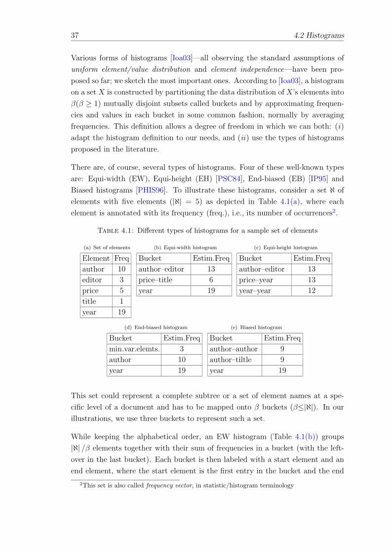
37 4.2 Histograms

Various forms of histograms [Ioa03]—all observing the standard assumptions of

uniform element/value distribution and element independence—have been pro-

posed so far; we sketch the most important ones. According to [Ioa03], a histogram

on a set X is constructed by partitioning the data distribution of X ’s elements into

β(β ≥ 1) mutually disjoint subsets called buckets and by approximating frequen-

cies and values in each bucket in some common fashion, normally by averaging

frequencies. This definition allows a degree of freedom in which we can both: (i)

adapt the histogram definition to our needs, and (ii) use the types of histograms

proposed in the literature.

There are, of course, several types of histograms. Four of these well-known types

are: Equi-width (EW), Equi-height (EH) [PSC84], End-biased (EB) [IP95] and

Biased histograms [PHIS96]. To illustrate these histograms, consider a set ℵ of

elements with five elements (|ℵ| = 5) as depicted in Table 4.1(a), where each

element is annotated with its frequency (freq.), i.e., its number of occurrences2.

Table 4.1: Different types of histograms for a sample set of elements

(a) Set of elements

Element Freq

author 10

editor 3

price 5

title 1

year 19

(b) Equi-width histogram

Bucket Estim.Freq

author–editor 13

price–title 6

year 19

(c) Equi-height histogram

Bucket Estim.Freq

author–editor 13

price–year 13

year–year 12

(d) End-biased histogram

Bucket Estim.Freq

min.var.elemts. 3

author 10

year 19

(e) Biased histogram

Bucket Estim.Freq

author–author 9

author–tiltle 9

year 19

This set could represent a complete subtree or a set of element names at a spe-

cific level of a document and has to be mapped onto β buckets (β≤|ℵ|). In our

illustrations, we use three buckets to represent such a set.

While keeping the alphabetical order, an EW histogram (Table 4.1(b)) groups

|ℵ| /β elements together with their sum of frequencies in a bucket (with the left-

over in the last bucket). Each bucket is then labeled with a start element and an

end element, where the start element is the first entry in the bucket and the end

2This set is also called frequency vector, in statistic/histogram terminology

4.2 Histograms 38

element is the last entry in the bucket. If a bucket holds only one entry, it will

have equal start and end elements.

In contrast, EH computes the sum S of the individual element frequencies and sets

S/ |ℵ| as an equal height. With this criterion, the entries of the original set are

partitioned in an order-preserving way into buckets (Table 4.1(c)). If the frequency

contribution of the end element is not fully contained in the bucket frequency (est.

freq.), this element will appear as the start element in the subsequent bucket

thereby spanning two (or more) buckets (see price–year and year–year buckets in

Table 4.1(c)).

The biased histogram types try to emphasize particular elements while they ap-

proximate the remaining elements. Some degrees of freedom are conceivable,

e.g., emphasizing elements with highest or highest/lowest frequencies or averag-

ing elements with minimum variance. In our example in Table 4.1(d), EB selects

|ℵ| − (β − 1) elements which exhibit the minimum variance and represents them

by a single bucket with their average frequency. The remaining β−1 elements are

represented by individual (singleton) buckets. Here, the EB histogram isolates the

elements author and year and averages the remaining elements (min. var. elemts)

in a bucket.

A Biased histogram (Table 4.1(e)) isolates the element with the highest frequency

(year) and approximates the remaining elements in an EH way.

The direct and straightforward application of histograms may not be appropriate

in all cases for XML data. In fact, some special situations exist in which histograms

cannot contribute to further compression. These cases are described and dealt with

as follows.

4.2.1 Histogram Application for XML

The first observation we have is that histograms have been originally designed

to numeric data and element names in an XML document are character strings.

Hence, we need a way to map element/attribute names to a numeric representa-

tion. Let us call it vocabulary. A vocabulary is a list of pairs “element-name:number”

which maps each distinct element/attribute name to a number. Because the num-

ber of distinct element/attribute names in an XML document is normally small,

39 4.2 Histograms

we only need one byte for the representation3. The number representing an el-

ement/attribute name is called VocabularyID (VocID). A vocabulary is thus a

prerequisite to apply histograms in XML documents. With a vocabulary, buckets

can now be represented by numbers.

The second observation is that for certain types of histograms (e.g., EB) some

buckets are not appropriately described. Almost every bucket is described by its

boundaries (e.g., author–editor and price–year). However, the “min.var.elemt.”

bucket in an EB histogram represents a set of elements with no explicit description.

In the other words, it is assumed that elements that are not in the singleton buckets

are in the “min.var.elemt.” bucket. However, for estimating path expressions, this

may be a problem for certain axes (e.g. descendant axis) and provoke a low quality

estimation.

For example, consider a path expression //a/b. To estimate such an expression,

we need to scan a summary looking for all sub-trees rooted by a and probe a b as a

child. If the children of these sub-trees are presented by an EB histogram, it may

happen that for one (or more) sub-tree with no b, the corresponding histogram will

report a non-zero estimation due to the semantic of “min.var.elemt.” bucket. This

is clearly a case of false-positive probe during the estimation process4. Therefore,

so as not to derive bad estimates we need, in this case, an explicit descriptor. Let

us call it MVBD – Min.Var. Bucket Descriptor.

The computation of MVBD is quite simple. Having a vocabulary and the list of

singleton buckets, we can build a (compressed) bit list of all elements inside of

the “min.var.elemt.” bucket. Additionally, we need the first and the last element

(in fact, their VocIDs) for MVBD. For example, consider that we have 3 elements

to be represented in the MVBD: j(VocID=10), o(15), and t(20). The MVBD is,

in this case, formed by (10:20,10000100001). Each bit position between 10 and

20 is represented by “1” if the element is in the MVBD, or “0”, otherwise5. The

resulting EB histograms with the MVBD is called EB-MVBD.

The last observation is related to very irregular HNS structures. In such HNS,

it is a common case to have one or two element names per sub-tree or level.

The effective application of histograms in such cases depends completely on the

element frequencies. If there exist varying frequencies (e.g., one element with a

3In our experiments, only treebank reaches 251 distinct element names, while other documentsnormally have a vocabulary varying from 40 to 170 entries. Therefore, one byte suffices torepresent element/attribute names of an XML document.

4This should be avoided because the estimation error will tend to be high.5For any practical implementation issue, we need only the last VocID and the bit list. In any

case, bit compression techniques can be applied.

4.3 LESS—Leaf-Elements-in-Subtree Summarization 40

frequency of 20, and another one with 2,000), histograms cannot help so much

under compression and accuracy point of views. Applying an EB histogram with

one bucket is equivalent to averaging the frequencies—giving 1,010—which might

yield a very low estimation quality. Applying a two-buckets EB histogram would

correspond to, strictly speaking, no histogram at all, but rather a “bar graph”.

In this case, we would have accurate estimations with no savings in storage. If

we use an EH histogram with a number of buckets greater than two, the waste of

storage space would be even higher, and accuracy might also suffer as well.

To remedy such a situation, a re-scan in the HNS or in the entire document—

depending on the approach implemented—is necessary to decide, based on the

number of subtrees with one or two element names and on their frequencies, which

histogram configuration to use. This is obviously the ideal method but it incurs an

excessive extra time to be computed turning out a parametric method. Therefore,

to cope with these cases in a pragmatic way, we do not apply histograms on

subtrees/levels with only one or two element names. We apply instead the same

bit list compression method used for MVBD and record the respective frequencies,

i.e., without averaging them.

4.3 LESS—Leaf-Elements-in-Subtree Summariza-

tion

LESS [AMFH08a] is a structural summary in which histograms are applied in

subtrees, specifically in their leaf elements. Histograms are annotated in every

root element of subtrees.

4.3.1 The Main Idea

The observation that child sets having the same element name as their parent fre-

quently exhibit a similar element distribution led to the development of the LESS

method. It assumes a certain stable repetition (reasonably uniform distribution)

of such patterns of parent-child sets. Hence, this property serves to save storage

space.

The resulting LESS can be considered as a tree consisting of the inner HNS nodes

and specific compacting structures. LESS can derive histograms which approx-

imate the distribution information of child sets. In this sense, a child set is a

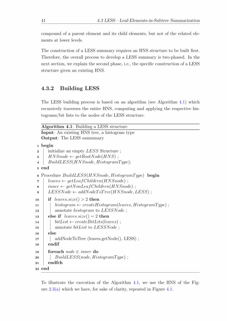
41 4.3 LESS—Leaf-Elements-in-Subtree Summarization

compound of a parent element and its child elements, but not of the related ele-

ments at lower levels.

The construction of a LESS summary requires an HNS structure to be built first.

Therefore, the overall process to develop a LESS summary is two-phased. In the

next section, we explain the second phase, i.e., the specific construction of a LESS

structure given an existing HNS.

4.3.2 Building LESS

The LESS building process is based on an algorithm (see Algorithm 4.1) which

recursively traverses the entire HNS, computing and applying the respective his-

tograms/bit lists to the nodes of the LESS structure.

Algorithm 4.1: Building a LESS structure

Input: An existing HNS tree, a histogram typeOutput: The LESS summmary

begin1

initialize an empty LESS Structure ;2

HNSnode← getRootNode(HNS) ;3

BuildLESS(HNSnode,HistogramType);4

end5

Procedure BuildLESS(HNSnode,HistogramType) begin6

leaves← getLeafChildren(HNSnode) ;7

inner ← getNonLeafChildren(HNSnode) ;8

LESSNode← addNodeToTree(HNSnode, LESS) ;9

if leaves.size() > 2 then10

histogram← createHistogram(leaves,HistogramType) ;11

annotate histogram to LESSNode ;12

else if leaves.size() = 2 then13

bitList← createBitLits(leaves) ;14

annotate bitList to LESSNode ;15

else16

addNodeToTree (leaves.getNode(), LESS) ;17

endif18

foreach node ∈ inner do19

BuildLESS(node,HistogramType) ;20

endfch21

end22

To illustrate the execution of the Algorithm 4.1, we use the HNS of the Fig-

ure 2.3(a) which we have, for sake of clarity, repeated in Figure 4.1.

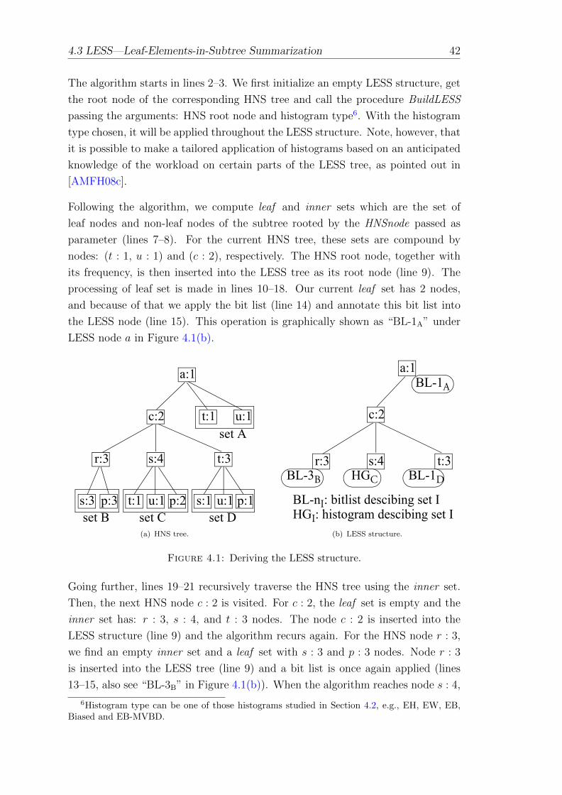
4.3 LESS—Leaf-Elements-in-Subtree Summarization 42

The algorithm starts in lines 2–3. We first initialize an empty LESS structure, get

the root node of the corresponding HNS tree and call the procedure BuildLESS

passing the arguments: HNS root node and histogram type6. With the histogram

type chosen, it will be applied throughout the LESS structure. Note, however, that

it is possible to make a tailored application of histograms based on an anticipated

knowledge of the workload on certain parts of the LESS tree, as pointed out in

[AMFH08c].

Following the algorithm, we compute leaf and inner sets which are the set of

leaf nodes and non-leaf nodes of the subtree rooted by the HNSnode passed as

parameter (lines 7–8). For the current HNS tree, these sets are compound by

nodes: (t : 1, u : 1) and (c : 2), respectively. The HNS root node, together with

its frequency, is then inserted into the LESS tree as its root node (line 9). The

processing of leaf set is made in lines 10–18. Our current leaf set has 2 nodes,

and because of that we apply the bit list (line 14) and annotate this bit list into

the LESS node (line 15). This operation is graphically shown as “BL-1A” under

LESS node a in Figure 4.1(b).

set Dset C

a:1

c:2 t:1 u:1

s:3 p:3 t:1 u:1

r:3 s:4

p:2 s:1 u:1

t:3

p:1

set A

set B(a) HNS tree.

a:1

c:2

r:3 s:4 t:3

BL-1A

BL-1DBL-3B HGC

BL-nI: bitlist descibing set IHGI: histogram descibing set I

(b) LESS structure.

Figure 4.1: Deriving the LESS structure.

Going further, lines 19–21 recursively traverse the HNS tree using the inner set.

Then, the next HNS node c : 2 is visited. For c : 2, the leaf set is empty and the

inner set has: r : 3, s : 4, and t : 3 nodes. The node c : 2 is inserted into the

LESS structure (line 9) and the algorithm recurs again. For the HNS node r : 3,

we find an empty inner set and a leaf set with s : 3 and p : 3 nodes. Node r : 3

is inserted into the LESS tree (line 9) and a bit list is once again applied (lines

13–15, also see “BL-3B” in Figure 4.1(b)). When the algorithm reaches node s : 4,

6Histogram type can be one of those histograms studied in Section 4.2, e.g., EH, EW, EB,Biased and EB-MVBD.

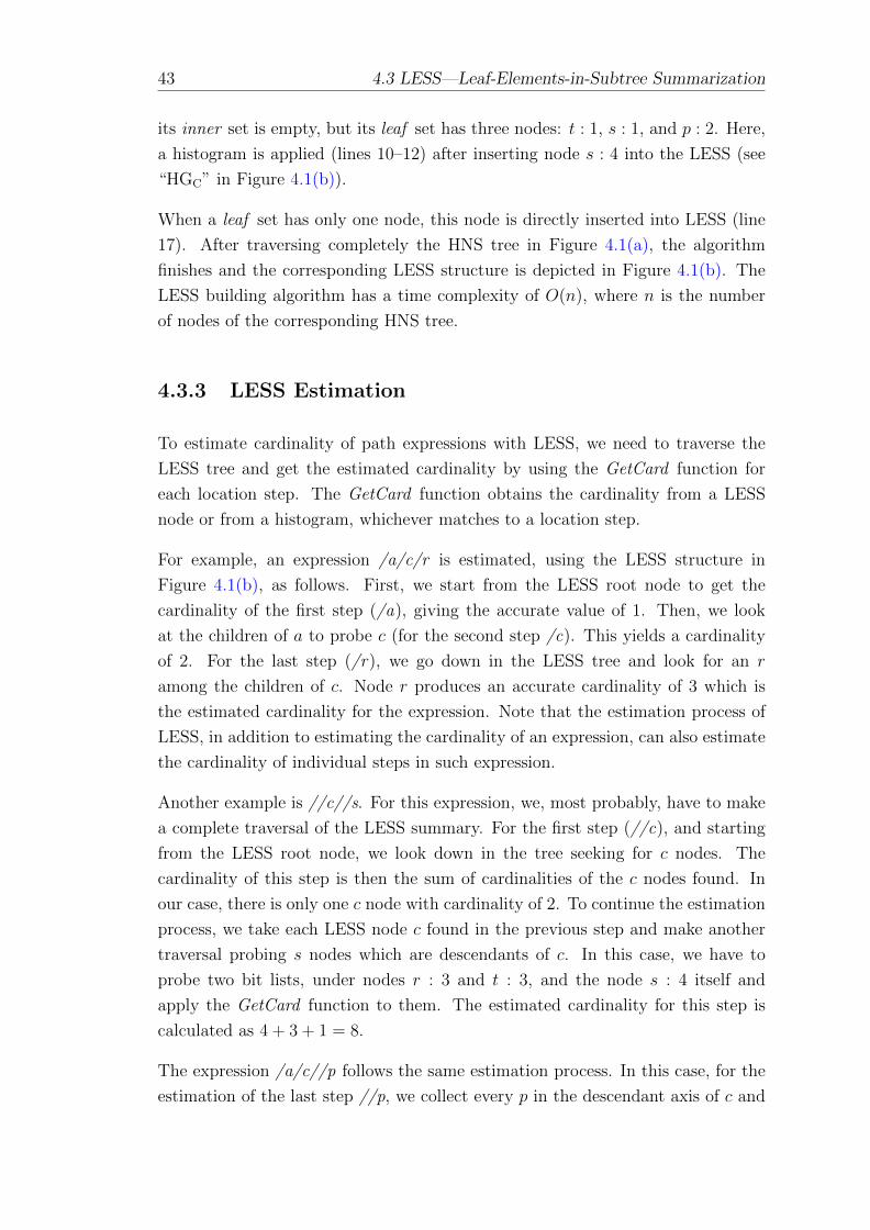
43 4.3 LESS—Leaf-Elements-in-Subtree Summarization

its inner set is empty, but its leaf set has three nodes: t : 1, s : 1, and p : 2. Here,

a histogram is applied (lines 10–12) after inserting node s : 4 into the LESS (see

“HGC” in Figure 4.1(b)).

When a leaf set has only one node, this node is directly inserted into LESS (line

17). After traversing completely the HNS tree in Figure 4.1(a), the algorithm

finishes and the corresponding LESS structure is depicted in Figure 4.1(b). The

LESS building algorithm has a time complexity of O(n), where n is the number

of nodes of the corresponding HNS tree.

4.3.3 LESS Estimation

To estimate cardinality of path expressions with LESS, we need to traverse the

LESS tree and get the estimated cardinality by using the GetCard function for

each location step. The GetCard function obtains the cardinality from a LESS

node or from a histogram, whichever matches to a location step.

For example, an expression /a/c/r is estimated, using the LESS structure in

Figure 4.1(b), as follows. First, we start from the LESS root node to get the

cardinality of the first step (/a), giving the accurate value of 1. Then, we look

at the children of a to probe c (for the second step /c). This yields a cardinality

of 2. For the last step (/r), we go down in the LESS tree and look for an r

among the children of c. Node r produces an accurate cardinality of 3 which is

the estimated cardinality for the expression. Note that the estimation process of

LESS, in addition to estimating the cardinality of an expression, can also estimate

the cardinality of individual steps in such expression.

Another example is //c//s. For this expression, we, most probably, have to make

a complete traversal of the LESS summary. For the first step (//c), and starting

from the LESS root node, we look down in the tree seeking for c nodes. The

cardinality of this step is then the sum of cardinalities of the c nodes found. In

our case, there is only one c node with cardinality of 2. To continue the estimation

process, we take each LESS node c found in the previous step and make another

traversal probing s nodes which are descendants of c. In this case, we have to

probe two bit lists, under nodes r : 3 and t : 3, and the node s : 4 itself and

apply the GetCard function to them. The estimated cardinality for this step is

calculated as 4 + 3 + 1 = 8.

The expression /a/c//p follows the same estimation process. In this case, for the

estimation of the last step //p, we collect every p in the descendant axis of c and

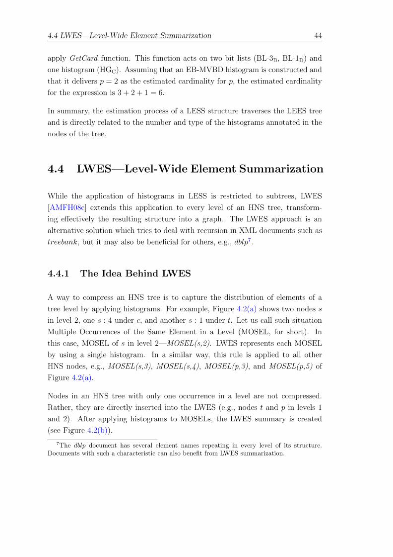
4.4 LWES—Level-Wide Element Summarization 44

apply GetCard function. This function acts on two bit lists (BL-3B, BL-1D) and

one histogram (HGC). Assuming that an EB-MVBD histogram is constructed and

that it delivers p = 2 as the estimated cardinality for p, the estimated cardinality

for the expression is 3 + 2 + 1 = 6.

In summary, the estimation process of a LESS structure traverses the LEES tree

and is directly related to the number and type of the histograms annotated in the

nodes of the tree.

4.4 LWES—Level-Wide Element Summarization

While the application of histograms in LESS is restricted to subtrees, LWES

[AMFH08c] extends this application to every level of an HNS tree, transform-

ing effectively the resulting structure into a graph. The LWES approach is an

alternative solution which tries to deal with recursion in XML documents such as

treebank, but it may also be beneficial for others, e.g., dblp7.

4.4.1 The Idea Behind LWES

A way to compress an HNS tree is to capture the distribution of elements of a

tree level by applying histograms. For example, Figure 4.2(a) shows two nodes s

in level 2, one s : 4 under c, and another s : 1 under t. Let us call such situation

Multiple Occurrences of the Same Element in a Level (MOSEL, for short). In

this case, MOSEL of s in level 2—MOSEL(s,2). LWES represents each MOSEL

by using a single histogram. In a similar way, this rule is applied to all other

HNS nodes, e.g., MOSEL(s,3), MOSEL(s,4), MOSEL(p,3), and MOSEL(p,5) of

Figure 4.2(a).

Nodes in an HNS tree with only one occurrence in a level are not compressed.

Rather, they are directly inserted into the LWES (e.g., nodes t and p in levels 1

and 2). After applying histograms to MOSELs, the LWES summary is created

(see Figure 4.2(b)).

7The dblp document has several element names repeating in every level of its structure.Documents with such a characteristic can also benefit from LWES summarization.

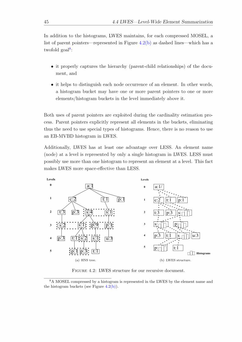
45 4.4 LWES—Level-Wide Element Summarization

In addition to the histograms, LWES maintains, for each compressed MOSEL, a

list of parent pointers—represented in Figure 4.2(b) as dashed lines—which has a

twofold goal8:

• it properly captures the hierarchy (parent-child relationships) of the docu-

ment, and

• it helps to distinguish each node occurrence of an element. In other words,

a histogram bucket may have one or more parent pointers to one or more

elements/histogram buckets in the level immediately above it.

Both uses of parent pointers are exploited during the cardinality estimation pro-

cess. Parent pointers explicitly represent all elements in the buckets, eliminating

thus the need to use special types of histograms. Hence, there is no reason to use

an EB-MVBD histogram in LWES.

Additionally, LWES has at least one advantage over LESS. An element name

(node) at a level is represented by only a single histogram in LWES. LESS must

possibly use more than one histogram to represent an element at a level. This fact

makes LWES more space-effective than LESS.

a:1

t:1c:2 p:1

p:9

t:3 s:4

s:2

s:1

p:3

p:3

u:3

p:1s:1

s:1s:2t:1

p:1 p:3 t:1

Levels

0

1

2

3

4

5

(a) HNS tree.

c:2 t:1 p:1

t:3 p:3 s:

s: p:

a:1/

p:3 u:3

p: t:1

t:1 s

Levels

0

1

2

3

4

5

Histograms

(b) LWES structure.

Figure 4.2: LWES structure for our recursive document.

8A MOSEL compressed by a histogram is represented in the LWES by the element name andthe histogram buckets (see Figure 4.2(b)).

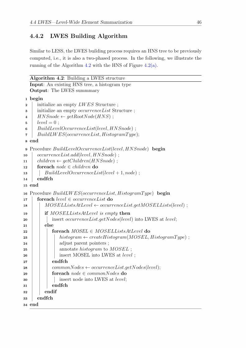
4.4 LWES—Level-Wide Element Summarization 46

4.4.2 LWES Building Algorithm

Similar to LESS, the LWES building process requires an HNS tree to be previously

computed, i.e., it is also a two-phased process. In the following, we illustrate the

running of the Algorithm 4.2 with the HNS of Figure 4.2(a).

Algorithm 4.2: Building a LWES structure

Input: An existing HNS tree, a histogram typeOutput: The LWES summmary

begin1

initialize an empty LWES Structure ;2

initialize an empty occurrenceList Structure ;3

HNSnode← getRootNode(HNS) ;4

level = 0 ;5

BuildLevelOccurrenceList(level,HNSnode) ;6

BuildLWES(occurrenceList,HistogramType);7

end8

Procedure BuildLevelOccurrenceList(level,HNSnode) begin9

occurrenceList.add(level,HNSnode) ;10

children← getChildren(HNSnode) ;11

foreach node ∈ children do12

BuildLevelOccurrenceList(level + 1, node) ;13

endfch14

end15

Procedure BuildLWES(occurrenceList,HistogramType) begin16

foreach level ∈ occurrenceList do17

MOSELListsAtLevel ← occurrenceList.getMOSELLists(level) ;18

if MOSELListsAtLevel is empty then19

insert occurrenceList.getNodes(level) into LWES at level;20

else21

foreach MOSEL ∈ MOSELListsAtLevel do22

histogram← createHistogram(MOSEL,HistogramType) ;23

adjust parent pointers ;24

annotate histogram to MOSEL ;25

insert MOSEL into LWES at level ;26

endfch27

commonNodes← occurrenceList.getNodes(level);28

foreach node ∈ commonNodes do29

insert node into LWES at level;30

endfch31

endif32

endfch33

end34

47 4.4 LWES—Level-Wide Element Summarization

To build an LWES summary, we need to first collect all nodes at each level of

the HNS tree. This is performed by procedure BuildLevelOccurrenceList (lines

9–15). Starting with the HNS root node, this procedure recursively creates an

occurrenceList for each level. Each occurrenceList contains all HNS nodes (line

10) at the respective level and is able to detect existing MOSELs in the level.

After creating occurrenceLists by traversing the HNS tree, we then have all the

data to summarize and construct an LWES structure (procedure BuildLWES in

lines 16–33). First of all, for each level in the occurrenceList, we must detect an

existing MOSEL in order to apply histograms and insert the MOSEL compressed

by a histogram into the LWES. The variable MOSELListsAtLevel stores all

MOSEL at a level retrieved by method getMOSELLists of occurrenceList. This

variable is, in fact, a list of MOSELs (line 18). If MOSELListsAtLevel is empty,

we can directly insert all nodes of occurrenceList into LWES, because there is no

possibility to apply a histogram (lines 19–20).

Therefore, at level 0 of the HNS tree (4.2(a)) there is only the root node which is

inserted into LWES level 0. The occurrenceList of level 1 has no MOSEL, just

common nodes which are also directly inserted in level 1 of LWES (see levels 0

and 1 of 4.2(b)).

However, we must apply histograms in existing MOSELs (lines 22–26). For

that, we create a histogram of a HistogramType for each MOSEL found in

MOSELListsAtLevel, In addition, parent pointers must be adjusted (line 24)

to reflect the correct relationship between the histogram buckets and their respec-

tive parents in the level above. Then, we insert the MOSEL together with parent

pointers into LWES (line 25–26).

The remaining nodes, i.e., nodes not belonging to a MOSEL, must also be inserted

into LWES (lines 28–30). MOSEL happens firstly at level 2 of the HNS tree.

In this case, there is a MOSEL(s, 2) and two common nodes t : 3 and p : 3.

Consequently, in level 2 of LWES there are three nodes: t, p and MOSEL(s, 2).

The latter is represented by the element name (s), the respective histogram and

parent pointers. In level 3 of the HNS tree, for example, there are two MOSELs.

Therefore, the corresponding level in LWES has also two nodes. This process

continues to be illustrated in levels 4 and 5 of the HNS tree.

After iterating throughout the levels, the algorithm finishes and the LWES sum-

mary is built as depicted in Figure 4.2(b). The LWES building algorithm has a

time complexity of O(2n) and a space complexity of O(n), where n is the number

of nodes of the corresponding HNS tree.

4.4 LWES—Level-Wide Element Summarization 48

4.4.3 Estimating Path Expression with LWES

The estimation process of LWES is based on a search in the LWES structure.

Similar to LESS, the GetCard function is also used to get the estimated cardinal-

ity of a path expression and the individual location steps of such an expression,

whether directly from common nodes or from histogram buckets annotated to the

compressed MOSELs. Therefore, for certain axes in a location step (e.g., //-axis),

the LWES structure should be, in the worst case, entirely traversed.

As an example, consider the expression /a/c/s/s posed on our recursive document

of Figure 2.2(a). This expression consists of location steps with only child axes.

The first step /a has a context node which is the document root. Then, we probe

the level 0 of the LWES for an a and obtain directly the step cardinality of 1. For

the second step /c, the level 1 is checked for a node c whose parent pointer points to

a. It is found with a cardinality of 2. The third step /s looks for a node s in level 2

with a parent pointer to c. This node s is a compressed MOSEL with a histogram.

The parent pointers link each histogram bucket to the respective parent node in

the level above. Hence, assuming that 2-bucket EB histograms were applied to the

LWES of Figure 4.2(b), we can find that the estimated cardinality for this step is

4. For the last step, another /s, the level 3 must be probed and the cardinality is

also obtained from a histogram. In this case, the cardinality of the step is 1 which

is the estimated cardinality of the expression9.

Therefore, for path expressions consisting of only child axis, the cardinality of the

expression is the cardinality of the last step. More formally, we have

Estim(/v1/v2/ · · · /vn) = GetCard(/vn) (4.4.1)

Now assume that a user wants to get all nodes p in a document. The corresponding

path expression is //p. This expression has a descendant axis and, in this case, the

estimation process triggers probes in every level of the LWES. In the other words,

the entire LWES structure is searched. At each level, a node p is probed and

the estimated cardinality is gathered (GetCard function applied). The estimated

cardinality for this expression is the sum of all GetCard application results. For

our example, the result is 20, if we use 2-bucket EB histograms10.

9If a 1-bucket EB histogram is applied to the LWES of the Figure 4.2(b), the estimatedcardinalities for the third and the last steps are 2.5 and 1.5, respectively. In this case, theestimated cardinality of the expression is 1.5.

10The result would be 15, if we had used 1-bucket EB histograms.

49 4.5 Discussion

Putting it in a more general way, we may say that every time a location step with

a descendant axis has to be estimated, the estimation result is the sum of the

partial results of every application of the GetCard function to the probed nodes.

More formally,

Estim(//v) =n∑

i=1

GetCard(vi) (4.4.2)

where vi is each probed node of v11.

To demonstrate the application possibilities of the Equation 4.4.1 and the Equa-

tion 4.4.2, we use the following expression /a/c//p/s. For the first two location

steps /a/c, Equation 4.4.1 applies directly, i.e., the estimated cardinality is the

cardinality of the second step which is 2. The application of Equation 4.4.2comes

with the third step (//p). Here, we must probe p nodes in LWES levels below the

level of node c, i.e., from level 2 down. For each node p that qualifies for the loca-

tion step, we sum its cardinalities to come up with the step cardinality which is 18.

Note that, for histograms—MOSEL(p)—buckets qualify if their parent pointers

track to c. In the last step /s, Equation 4.4.1 cannot be applied directly, because

the previous step contains a //-axis. In fact, we must look for an s in the level

immediately below and whose parent pointer points to one of the nodes gathered

in the previous step. Thus, /s has an estimated cardinality of 1.

4.5 Discussion

After having detailed our first two proposals on structural summarization of XML

documents, and in light of the points raised in Section 1.2.3, we must discuss

important issues related to them.

As positive points, we can highlight that LESS and LWES do not prune any

document path and the application of histograms better capture node distributions

in a document. This is in direct contrast to MT, which applies pruning, and PT

which prunes and averages frequencies of document nodes.

On the other hand, LESS and LWES may not scale for deeply structured docu-

ments in both storage size and estimation time. The possible reason is that LESS

and LWES summaries mirror somewhat the document tree structure thus making

11Note that, Equation 4.4.1 and Equation 4.4.2 apply also to the LESS estimation and, ingeneral, to all tree and graph structures to estimate these kinds of path expression. Here, wepresent a simple formalization of an intuitive knowledge.

4.5 Discussion 50

a correlation between the document structure and the summary structure. To

estimate //-axes, the estimation procedure must search most of the nodes of the

summary. The interplay of /and //-axes in a path expression makes the LWES

and LESS to memorize (save) some nodes for the next step estimation, thus aug-

menting the space (also most probably the time) complexity of the estimation

process.

Another negative point is that LESS and LWES can hardly estimate reverse axes

(parent and ancestor) or at most the estimation of such axes tend to yield a very

low estimation quality. The reasons for that is the coalescing of HNS nodes to

reflect their frequencies in parts of the document. Additionally, for ancestor axes

the memorization of nodes in the estimation process also applies.

Last point to be evaluated is the two-phased construction process, i.e., build the

HNS structure first and then the respective summary. Because of that, building

times may tend to be high for huge document sizes (see, for example, psd7003 and

uniprot documents in Table 6.1(a)).

On the other hand, for most practical cases12, LESS and LWES present themselves

(hopefully) as solutions for structural summarization of XML documents.

12Documents not deeply structured (e.g., up to 5 levels) and with a low degree of both struc-tural recursion and homonyms.

Chapter 5

EXsum—The Element-centered

XML Summarization

It is not only old and early impressions that deceive us;

the charms of novelty have the same power.

Blaise Pascal, French Mathematician, Philosopher and Physicist, 1623 – 1662. In: Thoughts

5.1 Introduction

This chapter presents EXsum, an Element-centered XML Summarization tech-

nique. In contrast to all approaches studied so far, EXsum does not follow the

strict tree hierarchy of an XML document. Rather, it concentrates on relation-

ships among element names (called spokes in EXsum) which capture the concept of

axes in a document and enable a direct (and simple) application in the estimation

process of path expressions.

This chapter is structured as follows. In Section 5.2, we introduce the motivation

which has driven the EXsum’s design. Section 5.3 presents the core idea and the

definition of EXsum structure. The EXsum construction algorithm is detailed in

Section 5.4 and the estimation procedures are studied in Section 5.6.

51

5.2 Motivation for EXsum 52

5.2 Motivation for EXsum

The design of EXsum has been motivated by three factors, in addition to accuracy:

fast access to the EXsum structure—avoiding a complete traversal to estimate lo-

cation steps, load on demand of parts of the structure—lowering the memory

footprint needed for the estimation process, and extensibility—which can be un-

derstood as the facility to easily aggregate more summarized data (e.g., parent

and ancestor axes summarization), and devise new estimation procedures.

These factors have been thought to be an answer to drawbacks found in the pub-

lished approaches and apply the lessons learned from the summarization structures

(basically, histograms) used in relational databases.

Relational databases allow summarization structures which are very concise and

have fast access. For example, consider a table with 20 columns having histograms

on 15 of them. To estimate a query referring to only 2 out of 15 columns, the

estimation process just needs to load 2 histograms into memory, lowering thus

the memory footprint necessary to estimation. Histograms, in turn, have fast

access—at most a binary search takes place—to deliver the estimated cardinality

of an expression. Therefore, we want to bring these important characteristics to

the XML summarization.

In all approaches published, one must traverse the corresponding structure to

gather the estimated cardinality of a location step (e.g., with descendant and/or

ancestor axes). This means that possibly the structure is searched many times

to get the final estimation result, hence, impacting the time for estimation and,

most likely, the overall optimization time. We want to avoid this behavior and

substitute it for a direct access to the summary whatever the axis estimated. In

other words, we want to limit the summary accesses to the number of location

steps in a path expression.

Last but not least, the majority of published summary structures are concerned

with the estimation of path expressions with /and //-axes, giving no room to

extend them to capture other axes or value distributions in XML documents.

We want a summary to be able to easily extend its structure in face of new

summarization needs.

After all, the structure with all these desirable characteristics must be as accurate

as possible to yield quality estimations. With these motivations in mind, we define

the EXsum structure in the next section.

53 5.3 The Gist of EXsum

5.3 The Gist of EXsum

To dive into the main idea behind EXsum, we need a little introspection and to

recall the basic definition of a tree. An XML document is a nodes’ hierarchy

which is represented by a tree in an XDBMS. Therefore, we assume the following

(recursive) definition of the tree [Har96]1.

Definition 5.1. Rooted Tree: An oriented rooted tree, or simply a rooted tree,

is a collection T of nodes which may be empty, otherwise it has the following

characteristics:

1. In T , a distinguished node exists r called root.

2. The T−r nodes form a set S = S1, S2, · · · , Sn where each Si is also a (rooted)

tree and is connected to r by an edge.

Each Si is called a subtree rooted in i. Each edge connecting two nodes a and

b correspond to a parent-child relationship between them, i.e., node a is called

parent (super-ordinate) of b—vice-versa, b is child (subordinate) of a. A tree with

n nodes has n− 1 edges. A leaf node is a node with no children.

We can derive from Definition 5.1 the following possible relationships (called axes

in XML terminology) among tree nodes, in addition to the parent-child relation-

ship.

• Ancestor : A node a is an ancestor of node b if a can be reached from b by

following the parent relationship.

• Descendant : A node a is an descendant of node b if a can be reached from

b by following the child relationship.

• Sibling : Two nodes a and b are considered siblings if they are children of a

common parent node.

The definition of the structure of an XML document described in [W3C98, W3C06]

and the path expressions syntax studied in Section 2.2.1 are compliant with the

Definition 5.1, which additionally defined two other axes: following:: and preced-

ing::. Therefore, we can reach the following observation.

1Translated into English and rephrased by the author.

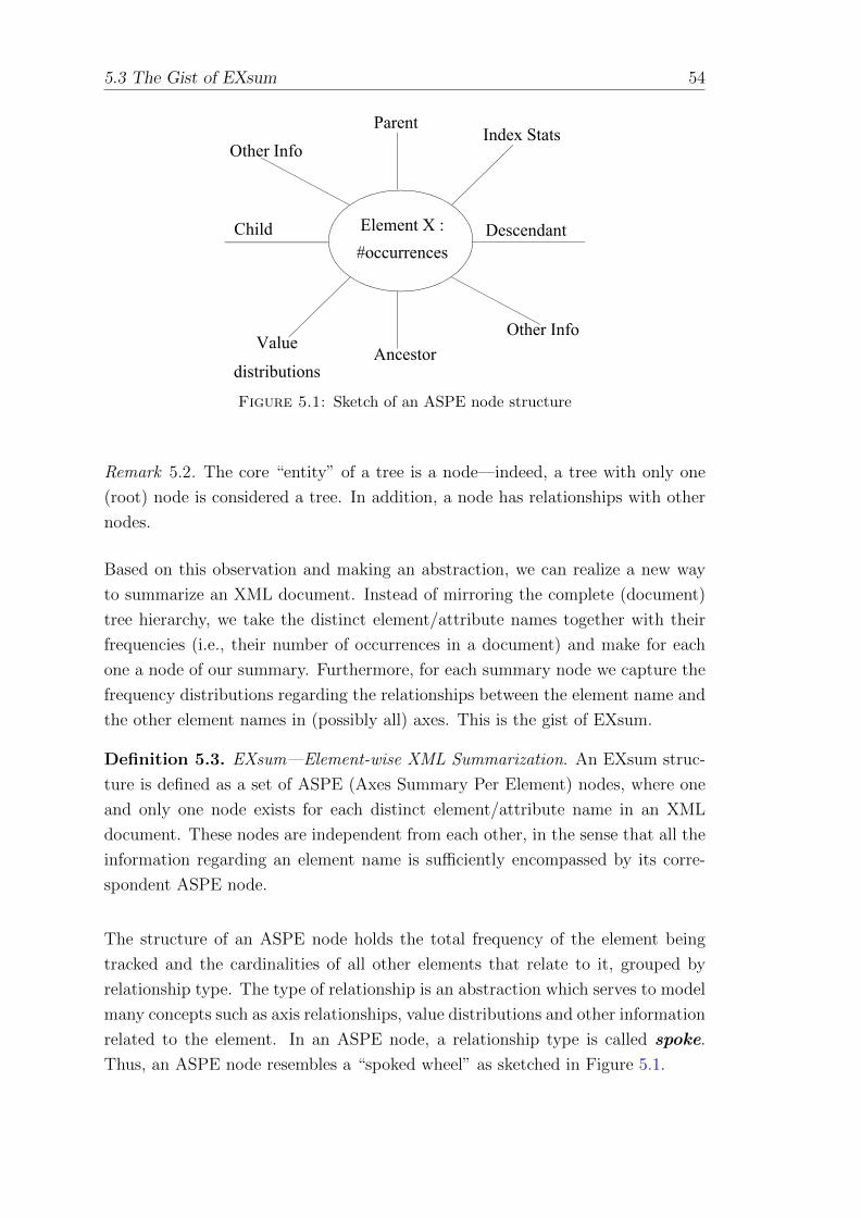
5.3 The Gist of EXsum 54

Element X : #occurrences

Parent

Ancestor

DescendantChild

Index Stats

Value

distributions

Other Info

Other Info

Figure 5.1: Sketch of an ASPE node structure

Remark 5.2. The core “entity” of a tree is a node—indeed, a tree with only one

(root) node is considered a tree. In addition, a node has relationships with other

nodes.

Based on this observation and making an abstraction, we can realize a new way

to summarize an XML document. Instead of mirroring the complete (document)

tree hierarchy, we take the distinct element/attribute names together with their

frequencies (i.e., their number of occurrences in a document) and make for each

one a node of our summary. Furthermore, for each summary node we capture the

frequency distributions regarding the relationships between the element name and

the other element names in (possibly all) axes. This is the gist of EXsum.

Definition 5.3. EXsum—Element-wise XML Summarization. An EXsum struc-

ture is defined as a set of ASPE (Axes Summary Per Element) nodes, where one

and only one node exists for each distinct element/attribute name in an XML

document. These nodes are independent from each other, in the sense that all the

information regarding an element name is sufficiently encompassed by its corre-

spondent ASPE node.

The structure of an ASPE node holds the total frequency of the element being

tracked and the cardinalities of all other elements that relate to it, grouped by

relationship type. The type of relationship is an abstraction which serves to model

many concepts such as axis relationships, value distributions and other information

related to the element. In an ASPE node, a relationship type is called spoke.

Thus, an ASPE node resembles a “spoked wheel” as sketched in Figure 5.1.

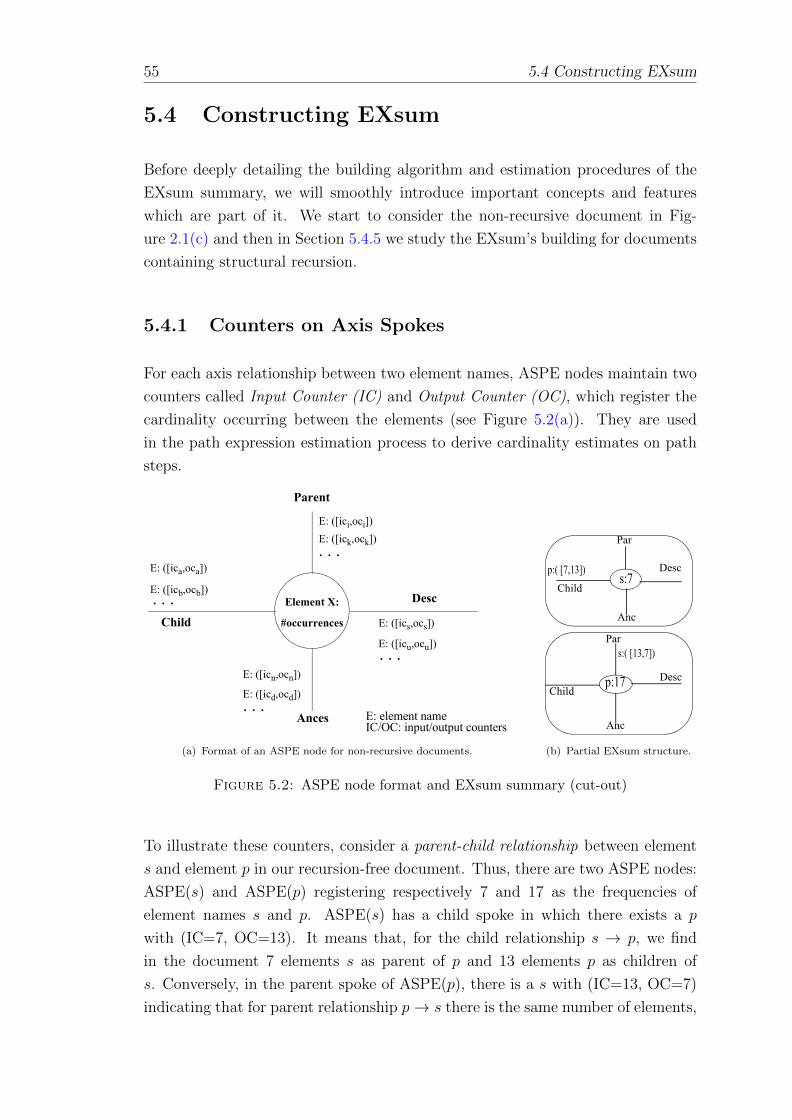
55 5.4 Constructing EXsum

5.4 Constructing EXsum

Before deeply detailing the building algorithm and estimation procedures of the

EXsum summary, we will smoothly introduce important concepts and features

which are part of it. We start to consider the non-recursive document in Fig-

ure 2.1(c) and then in Section 5.4.5 we study the EXsum’s building for documents

containing structural recursion.

5.4.1 Counters on Axis Spokes

For each axis relationship between two element names, ASPE nodes maintain two

counters called Input Counter (IC) and Output Counter (OC), which register the

cardinality occurring between the elements (see Figure 5.2(a)). They are used

in the path expression estimation process to derive cardinality estimates on path

steps.

Element X:

#occurrences

Parent

Ances

Desc

Child

E: ([ici,oci])E: ([ick,ock])

E: element name

. . .

E: ([icn,ocn])

E: ([icd,ocd]). . .

E: ([ica,oca])

E: ([icb,ocb]). . . E: ([ics,ocs])

E: ([icu,ocu]). . .

IC/OC: input/output counters

(a) Format of an ASPE node for non-recursive documents.

s:7

Anc

Par

Child

Descp:( [7,13])

p:17

Anc

Par

ChildDesc

s:( [13,7])

(b) Partial EXsum structure.

Figure 5.2: ASPE node format and EXsum summary (cut-out)

To illustrate these counters, consider a parent-child relationship between element

s and element p in our recursion-free document. Thus, there are two ASPE nodes:

ASPE(s) and ASPE(p) registering respectively 7 and 17 as the frequencies of

element names s and p. ASPE(s) has a child spoke in which there exists a p

with (IC=7, OC=13). It means that, for the child relationship s → p, we find

in the document 7 elements s as parent of p and 13 elements p as children of

s. Conversely, in the parent spoke of ASPE(p), there is a s with (IC=13, OC=7)

indicating that for parent relationship p→ s there is the same number of elements,

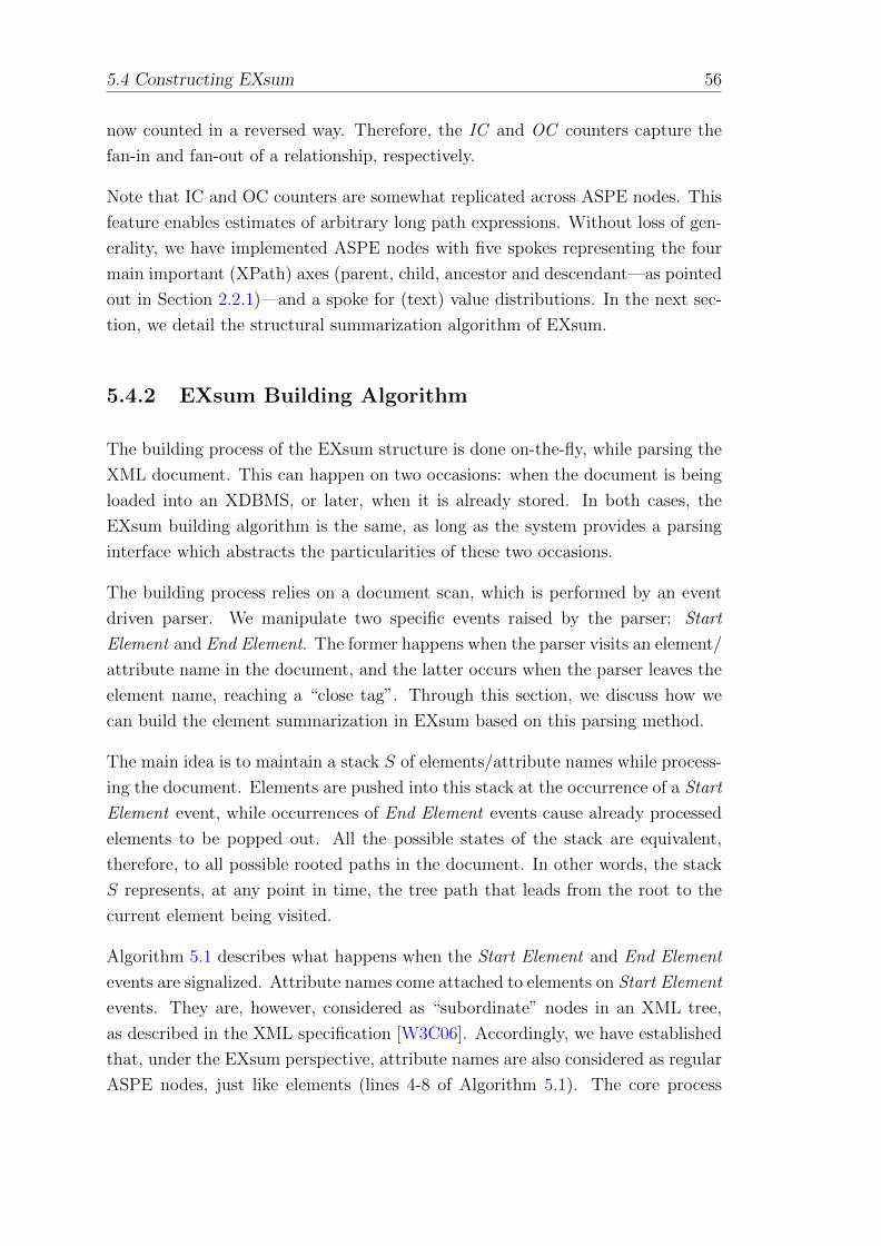
5.4 Constructing EXsum 56

now counted in a reversed way. Therefore, the IC and OC counters capture the

fan-in and fan-out of a relationship, respectively.

Note that IC and OC counters are somewhat replicated across ASPE nodes. This

feature enables estimates of arbitrary long path expressions. Without loss of gen-

erality, we have implemented ASPE nodes with five spokes representing the four

main important (XPath) axes (parent, child, ancestor and descendant—as pointed

out in Section 2.2.1)—and a spoke for (text) value distributions. In the next sec-

tion, we detail the structural summarization algorithm of EXsum.

5.4.2 EXsum Building Algorithm

The building process of the EXsum structure is done on-the-fly, while parsing the

XML document. This can happen on two occasions: when the document is being

loaded into an XDBMS, or later, when it is already stored. In both cases, the

EXsum building algorithm is the same, as long as the system provides a parsing

interface which abstracts the particularities of these two occasions.

The building process relies on a document scan, which is performed by an event

driven parser. We manipulate two specific events raised by the parser: Start

Element and End Element. The former happens when the parser visits an element/

attribute name in the document, and the latter occurs when the parser leaves the

element name, reaching a “close tag”. Through this section, we discuss how we

can build the element summarization in EXsum based on this parsing method.

The main idea is to maintain a stack S of elements/attribute names while process-

ing the document. Elements are pushed into this stack at the occurrence of a Start

Element event, while occurrences of End Element events cause already processed

elements to be popped out. All the possible states of the stack are equivalent,

therefore, to all possible rooted paths in the document. In other words, the stack

S represents, at any point in time, the tree path that leads from the root to the

current element being visited.

Algorithm 5.1 describes what happens when the Start Element and End Element

events are signalized. Attribute names come attached to elements on Start Element

events. They are, however, considered as “subordinate” nodes in an XML tree,

as described in the XML specification [W3C06]. Accordingly, we have established

that, under the EXsum perspective, attribute names are also considered as regular

ASPE nodes, just like elements (lines 4-8 of Algorithm 5.1). The core process

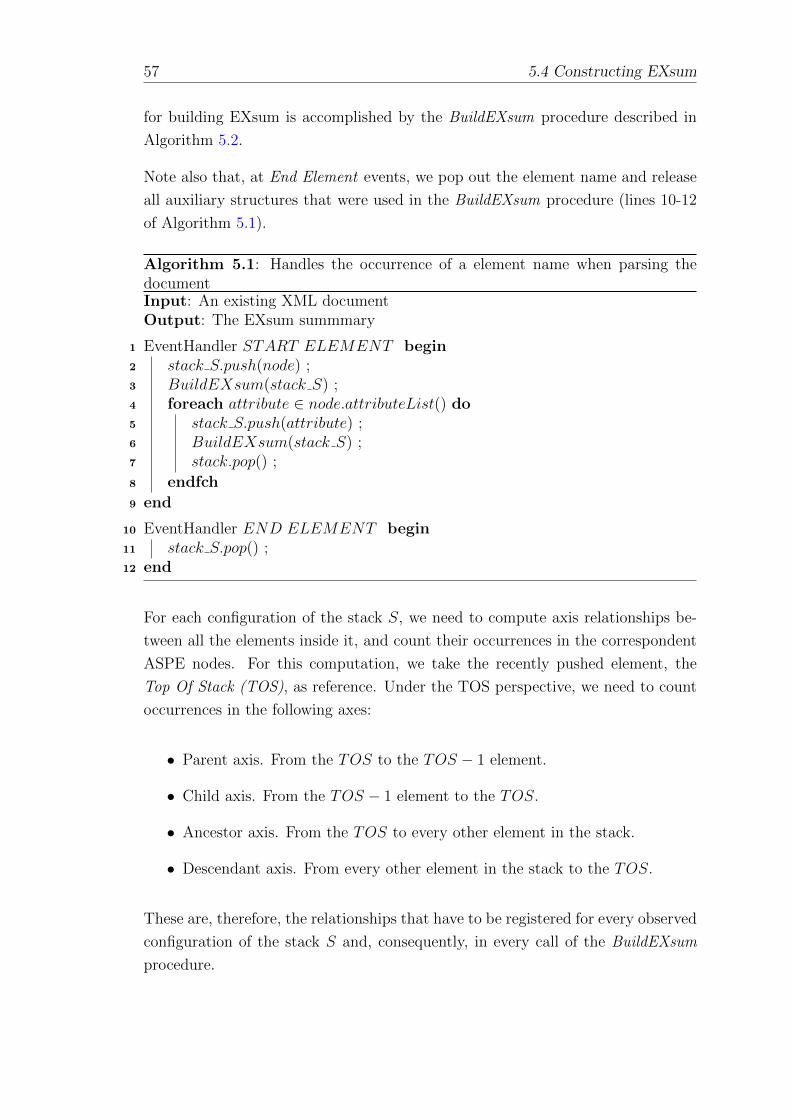
57 5.4 Constructing EXsum

for building EXsum is accomplished by the BuildEXsum procedure described in

Algorithm 5.2.

Note also that, at End Element events, we pop out the element name and release

all auxiliary structures that were used in the BuildEXsum procedure (lines 10-12

of Algorithm 5.1).

Algorithm 5.1: Handles the occurrence of a element name when parsing thedocumentInput: An existing XML documentOutput: The EXsum summmary

EventHandler START ELEMENT begin1

stack S.push(node) ;2

BuildEXsum(stack S) ;3

foreach attribute ∈ node.attributeList() do4

stack S.push(attribute) ;5

BuildEXsum(stack S) ;6

stack.pop() ;7

endfch8

end9

EventHandler END ELEMENT begin10

stack S.pop() ;11

end12

For each configuration of the stack S, we need to compute axis relationships be-

tween all the elements inside it, and count their occurrences in the correspondent

ASPE nodes. For this computation, we take the recently pushed element, the

Top Of Stack (TOS), as reference. Under the TOS perspective, we need to count

occurrences in the following axes:

• Parent axis. From the TOS to the TOS − 1 element.

• Child axis. From the TOS − 1 element to the TOS.

• Ancestor axis. From the TOS to every other element in the stack.

• Descendant axis. From every other element in the stack to the TOS.

These are, therefore, the relationships that have to be registered for every observed

configuration of the stack S and, consequently, in every call of the BuildEXsum

procedure.

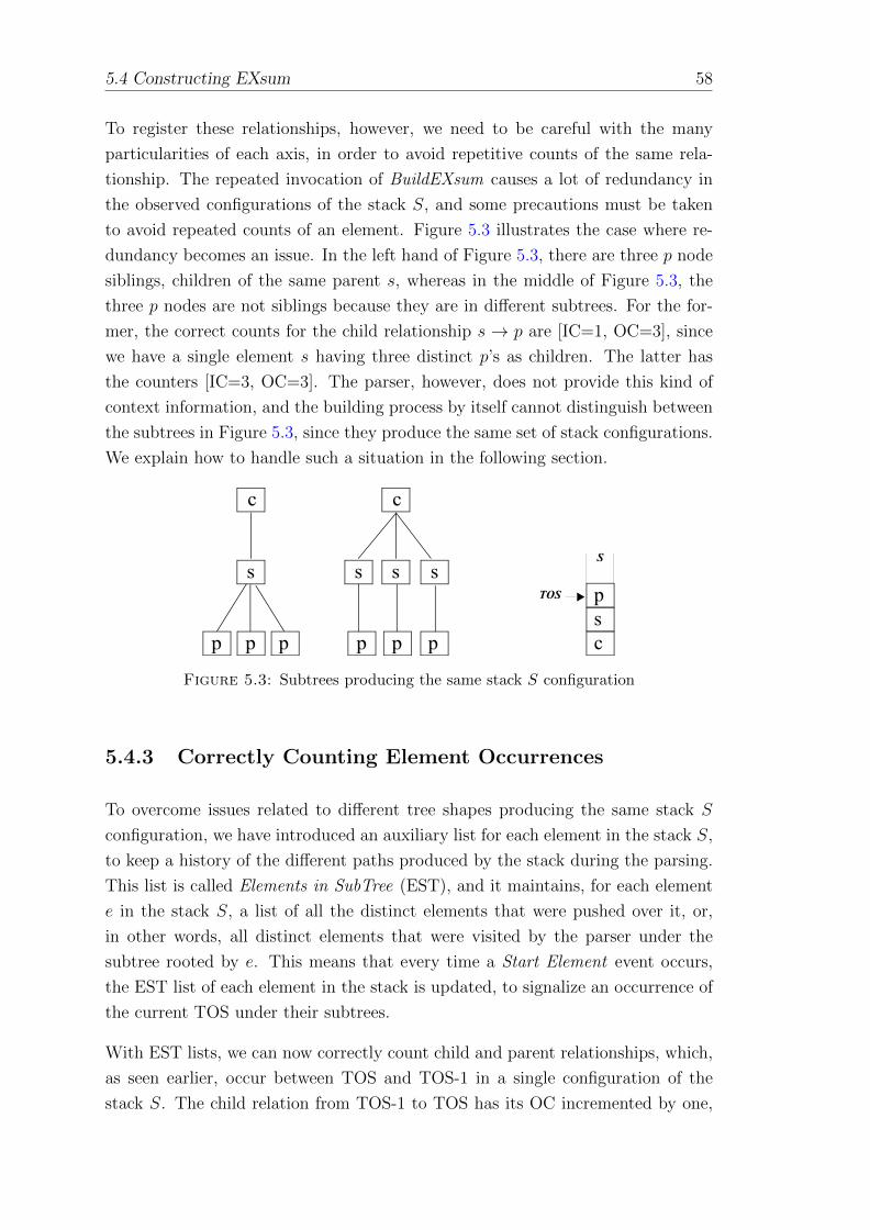
5.4 Constructing EXsum 58

To register these relationships, however, we need to be careful with the many

particularities of each axis, in order to avoid repetitive counts of the same rela-

tionship. The repeated invocation of BuildEXsum causes a lot of redundancy in

the observed configurations of the stack S, and some precautions must be taken

to avoid repeated counts of an element. Figure 5.3 illustrates the case where re-

dundancy becomes an issue. In the left hand of Figure 5.3, there are three p node

siblings, children of the same parent s, whereas in the middle of Figure 5.3, the

three p nodes are not siblings because they are in different subtrees. For the for-

mer, the correct counts for the child relationship s → p are [IC=1, OC=3], since

we have a single element s having three distinct p’s as children. The latter has

the counters [IC=3, OC=3]. The parser, however, does not provide this kind of

context information, and the building process by itself cannot distinguish between

the subtrees in Figure 5.3, since they produce the same set of stack configurations.

We explain how to handle such a situation in the following section.

c

p p

s

p

c

p p

s

p

ss

csp

S

TOS

Figure 5.3: Subtrees producing the same stack S configuration

5.4.3 Correctly Counting Element Occurrences

To overcome issues related to different tree shapes producing the same stack S

configuration, we have introduced an auxiliary list for each element in the stack S,

to keep a history of the different paths produced by the stack during the parsing.

This list is called Elements in SubTree (EST), and it maintains, for each element

e in the stack S, a list of all the distinct elements that were pushed over it, or,

in other words, all distinct elements that were visited by the parser under the

subtree rooted by e. This means that every time a Start Element event occurs,

the EST list of each element in the stack is updated, to signalize an occurrence of

the current TOS under their subtrees.

With EST lists, we can now correctly count child and parent relationships, which,

as seen earlier, occur between TOS and TOS-1 in a single configuration of the

stack S. The child relation from TOS-1 to TOS has its OC incremented by one,

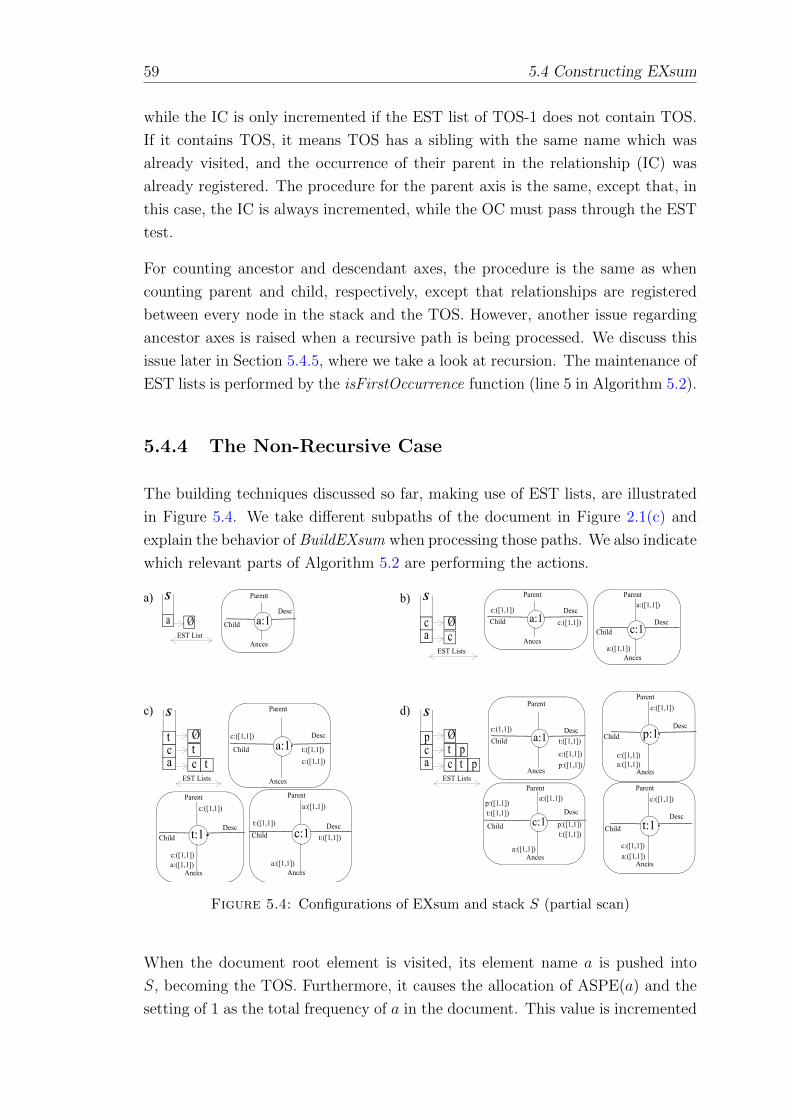
59 5.4 Constructing EXsum

while the IC is only incremented if the EST list of TOS-1 does not contain TOS.

If it contains TOS, it means TOS has a sibling with the same name which was

already visited, and the occurrence of their parent in the relationship (IC) was

already registered. The procedure for the parent axis is the same, except that, in

this case, the IC is always incremented, while the OC must pass through the EST

test.

For counting ancestor and descendant axes, the procedure is the same as when

counting parent and child, respectively, except that relationships are registered

between every node in the stack and the TOS. However, another issue regarding

ancestor axes is raised when a recursive path is being processed. We discuss this

issue later in Section 5.4.5, where we take a look at recursion. The maintenance of

EST lists is performed by the isFirstOccurrence function (line 5 in Algorithm 5.2).

5.4.4 The Non-Recursive Case

The building techniques discussed so far, making use of EST lists, are illustrated

in Figure 5.4. We take different subpaths of the document in Figure 2.1(c) and

explain the behavior of BuildEXsum when processing those paths. We also indicate

which relevant parts of Algorithm 5.2 are performing the actions.

act

S

c tt

EST Lists

c)

a

S

ØEST List

a)

a:1Child

Desc

Parent

Ancesac

S

cØ

EST Lists

b)a:1Child

Desc

Parent

Ancesc:1Child

Desc

Parent

Ances

c:([1,1])a:([1,1])

Øa:1Child

Desc

Parent

Ances

c:1ChildDesc

Parent

Ances

c:([1,1])

a:([1,1])

t:1ChildDesc

Parent

Ances

c:([1,1])

a:([1,1])

t:([1,1])

t:([1,1])

acp

S

c tt

EST Lists

d)

Øp

p

a:1ChildDesc

Parent

Ances

c:1Child

Desc

Parent

Ances

c:(1,1])

a:([1,1])

t:1ChildDesc

Parent

Ances

c:([1,1])

a:([1,1])

t:([1,1])

c:([1,1])p:([1,1])

p:([1,1])

p:1ChildDesc

Parent

Ances

c:([1,1])

a:([1,1])

c:([1,1])

a:([1,1])

c:([1,1])

a:([1,1])

t:([1,1])

c:([1,1])

t:([1,1])

t:([1,1])p:([1,1])

a:([1,1]) c:([1,1])

c:([1,1])

Figure 5.4: Configurations of EXsum and stack S (partial scan)

When the document root element is visited, its element name a is pushed into

S, becoming the TOS. Furthermore, it causes the allocation of ASPE(a) and the

setting of 1 as the total frequency of a in the document. This value is incremented

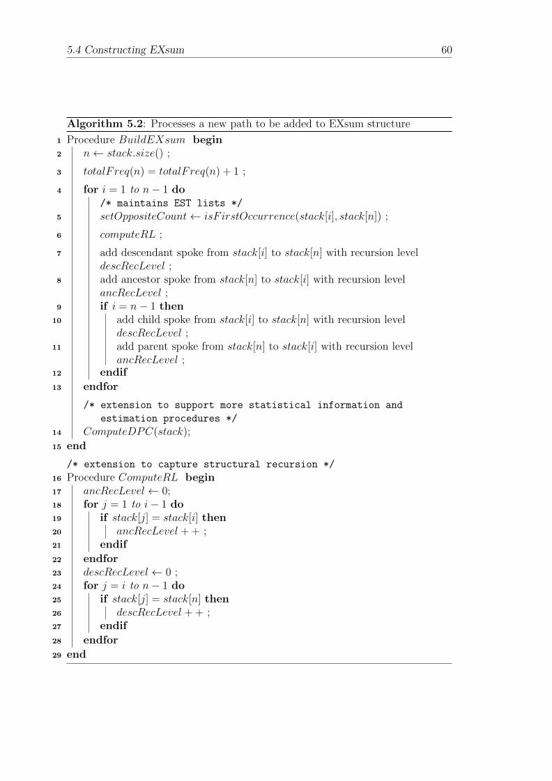
5.4 Constructing EXsum 60

Algorithm 5.2: Processes a new path to be added to EXsum structure

Procedure BuildEXsum begin1

n← stack.size() ;2

totalFreq(n) = totalFreq(n) + 1 ;3

for i = 1 to n− 1 do4

/* maintains EST lists */

setOppositeCount← isF irstOccurrence(stack[i], stack[n]) ;5

computeRL ;6

add descendant spoke from stack[i] to stack[n] with recursion level7

descRecLevel ;add ancestor spoke from stack[n] to stack[i] with recursion level8

ancRecLevel ;if i = n− 1 then9

add child spoke from stack[i] to stack[n] with recursion level10

descRecLevel ;add parent spoke from stack[n] to stack[i] with recursion level11

ancRecLevel ;endif12

endfor13

/* extension to support more statistical information and

estimation procedures */

ComputeDPC(stack);14

end15

/* extension to capture structural recursion */

Procedure ComputeRL begin16

ancRecLevel← 0;17

for j = 1 to i− 1 do18

if stack[j] = stack[i] then19

ancRecLevel + + ;20

endif21

endfor22

descRecLevel← 0 ;23

for j = i to n− 1 do24

if stack[j] = stack[n] then25

descRecLevel + + ;26

endif27

endfor28

end29

61 5.4 Constructing EXsum

for the TOS in every execution of BuildEXsum, as seen in line 13 of Algorithm 5.2.

After that, an empty EST list is allocated for a. The current state of the EXsum

summary is shown in Figure 5.4(a).

In the next step, a node with element name c is reached and pushed into S. Because

ASPE(c) is not present, it is created and the related axes information is added to

a and c as follows. The algorithm needs to adjust IC/OC counters in ASPE(a)

and in ASPE(c). Since this is the first time that c appears under a, the EST list

of a includes c and signalizes that it was not present before (isFirstOccurrence in

line 3). The function isFirstOccurrence(x,y) checks if this is the first occurrence

of the node y under the subtree rooted by node x, by looking for the node y in

the EST list of x. If no occurrence is found, it adds y to the list and returns true.

In our case, since the function returns true, both IC and OC are set, resulting in

[IC=1, OC=1] for a → c in child and descendant axes. Similarly, c → a ends up

with [IC=1,OC=1] in the parent and ancestor spokes. The summary now looks

like the one in Figure 5.4(b).

It is important to note that every child relationship is also a descendant one, and

the same is valid for parent and ancestor. This comes from the XPath specification

[W3C07], where a descendant axis relationship is defined as “the transitive closure

of the child axis; it contains the descendants of the context node (the children, the

children of the children, and so on)”, and the definition of ancestor follows in a

similar way2. Therefore, when registering child and parent relationships, EXsum

also considers them as descendant and ancestor.

Continuing the document scan, a node with element name t is now visited (S =

[a, c, t]) ( Figure 5.4(c)). Again, t is pushed into S, ASPE(t) is created, and the

axis relationships between t and the other path elements c and a are updated.

Note that child and parent will only be set between t and c. The EST lists of a

and c now contain a t, and again both lists report that it is the first occurrence.

Thus, the counts [IC=1, OC=1] are registered for ancestor and descendant axes

of a ↔ t and c ↔ t (lines 5 and 6). Additionally, child and parent are also set

with the same values for c↔ t (lines 8 and 9).

Since t has no children, an end element event is signalized and t is popped out

from S. This process is iterated when the scan reaches the fourth element p

(S = [a, c, p]) and counters are adjusted in a ↔ p and c ↔ p, in the same way as

2According to the XPath specification [W3C07], the ancestor axis is defined as “the transitiveclosure of the parent axis; it contains the ancestors of the context node (the parent, the parent ofthe parent, and so on)”

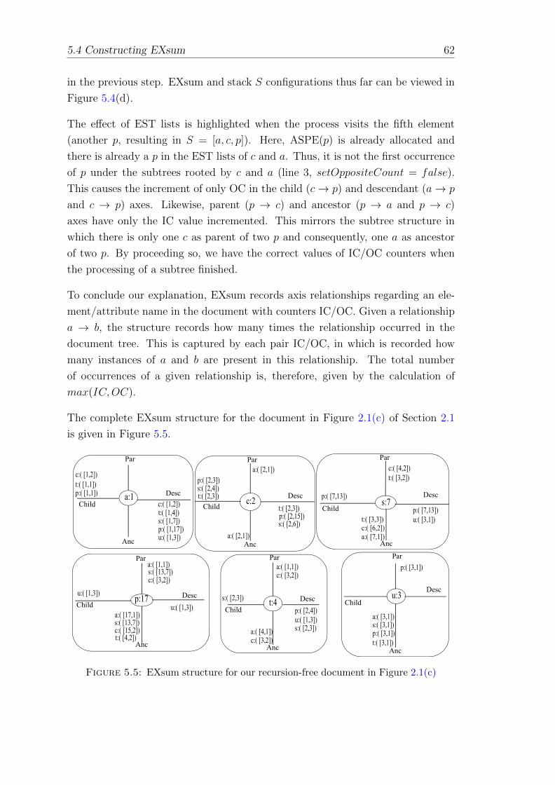
5.4 Constructing EXsum 62

in the previous step. EXsum and stack S configurations thus far can be viewed in

Figure 5.4(d).

The effect of EST lists is highlighted when the process visits the fifth element

(another p, resulting in S = [a, c, p]). Here, ASPE(p) is already allocated and

there is already a p in the EST lists of c and a. Thus, it is not the first occurrence

of p under the subtrees rooted by c and a (line 3, setOppositeCount = false).

This causes the increment of only OC in the child (c→ p) and descendant (a→ p

and c → p) axes. Likewise, parent (p → c) and ancestor (p → a and p → c)

axes have only the IC value incremented. This mirrors the subtree structure in

which there is only one c as parent of two p and consequently, one a as ancestor

of two p. By proceeding so, we have the correct values of IC/OC counters when

the processing of a subtree finished.

To conclude our explanation, EXsum records axis relationships regarding an ele-

ment/attribute name in the document with counters IC/OC. Given a relationship

a → b, the structure records how many times the relationship occurred in the

document tree. This is captured by each pair IC/OC, in which is recorded how

many instances of a and b are present in this relationship. The total number

of occurrences of a given relationship is, therefore, given by the calculation of

max(IC,OC).

The complete EXsum structure for the document in Figure 2.1(c) of Section 2.1

is given in Figure 5.5.

s:7

Anc

Par

Child

Descp:( [7,13])

p:( [7,13])t:( [3,3])c:( [6,2])a:( [7,1])

c:( [4,2])

t:4

Anc

Par

ChildDesc

c:( [3,2])

c:( [3,2])

c:2

Anc

Par

ChildDesct:( [2,3])

p:( [2,3])s:( [2,4])

a:( [2,1])

p:( [2,15])s:( [2,6])

t:( [2,3])

p:17

Anc

Par

ChildDesc

a:( [17,1])s:( [13,7])c:( [15,2])

s:( [13,7])c:( [3,2])

a:( [4,1])

u:( [1,3])

u:( [1,3])

a:1

Anc

Par

ChildDesc

t:( [1,4])s:( [1,7])p:( [1,17])

p:( [1,1])t:( [1,1])c:( [1,2])

u:3

Anc

Par

Child

Desc

a:( [3,1])

p:( [3,1])

t:( [3,1])

s:( [3,1])

a:( [1,1])

s:( [2,3])

a:( [1,1])

t:( [4,2])

u:( [1,3])

u:( [3,1])

u:( [1,3])p:( [2,4])

t:( [3,2])

p:( [3,1])

c:( [1,2])

a:( [2,1])

s:( [2,3])

Figure 5.5: EXsum structure for our recursion-free document in Figure 2.1(c)

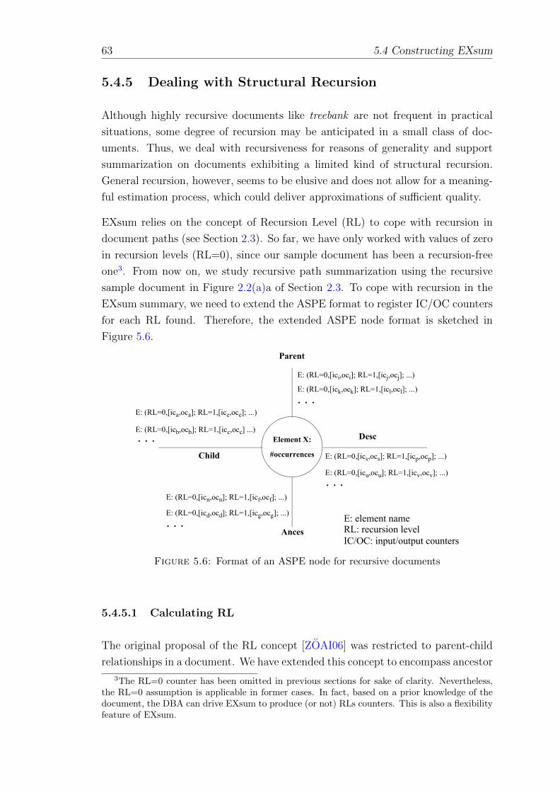
63 5.4 Constructing EXsum

5.4.5 Dealing with Structural Recursion

Although highly recursive documents like treebank are not frequent in practical

situations, some degree of recursion may be anticipated in a small class of doc-

uments. Thus, we deal with recursiveness for reasons of generality and support

summarization on documents exhibiting a limited kind of structural recursion.

General recursion, however, seems to be elusive and does not allow for a meaning-

ful estimation process, which could deliver approximations of sufficient quality.

EXsum relies on the concept of Recursion Level (RL) to cope with recursion in

document paths (see Section 2.3). So far, we have only worked with values of zero

in recursion levels (RL=0), since our sample document has been a recursion-free

one3. From now on, we study recursive path summarization using the recursive

sample document in Figure 2.2(a)a of Section 2.3. To cope with recursion in the

EXsum summary, we need to extend the ASPE format to register IC/OC counters

for each RL found. Therefore, the extended ASPE node format is sketched in

Figure 5.6.

Element X:

#occurrences

Parent

Ances

Desc

Child

E: (RL=0,[ici,oci]; RL=1,[icj,ocj]; ...)

E: (RL=0,[ick,ock]; RL=1,[icl,ocl]; ...)

E: element name

. . .

E: (RL=0,[icn,ocn]; RL=1,[icf,ocf]; ...)

E: (RL=0,[icd,ocd]; RL=1,[icg,ocg]; ...). . .

E: (RL=0,[ica,oca]; RL=1,[ice,oce]; ...)

E: (RL=0,[icb,ocb]; RL=1,[icc,occ] ...). . . E: (RL=0,[ics,ocs]; RL=1,[icp,ocp]; ...)

E: (RL=0,[icu,ocu]; RL=1,[icv,ocv]; ...). . .

RL: recursion levelIC/OC: input/output counters

Figure 5.6: Format of an ASPE node for recursive documents

5.4.5.1 Calculating RL

The original proposal of the RL concept [ZOAI06] was restricted to parent-child

relationships in a document. We have extended this concept to encompass ancestor

3The RL=0 counter has been omitted in previous sections for sake of clarity. Nevertheless,the RL=0 assumption is applicable in former cases. In fact, based on a prior knowledge of thedocument, the DBA can drive EXsum to produce (or not) RLs counters. This is also a flexibilityfeature of EXsum.

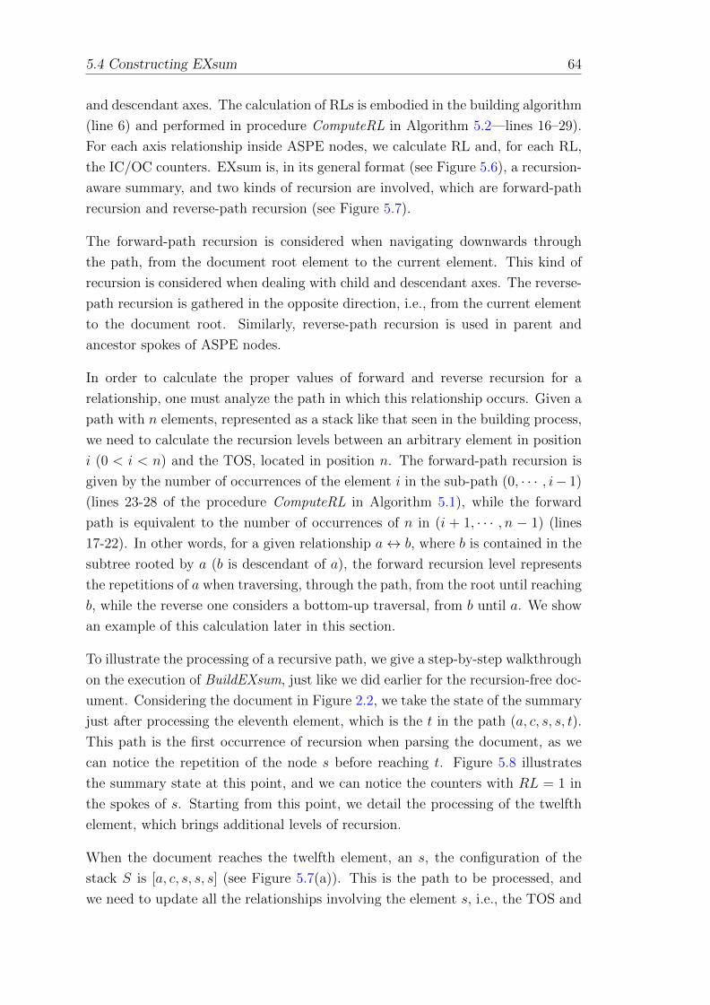
5.4 Constructing EXsum 64

and descendant axes. The calculation of RLs is embodied in the building algorithm

(line 6) and performed in procedure ComputeRL in Algorithm 5.2—lines 16–29).

For each axis relationship inside ASPE nodes, we calculate RL and, for each RL,

the IC/OC counters. EXsum is, in its general format (see Figure 5.6), a recursion-

aware summary, and two kinds of recursion are involved, which are forward-path

recursion and reverse-path recursion (see Figure 5.7).

The forward-path recursion is considered when navigating downwards through

the path, from the document root element to the current element. This kind of

recursion is considered when dealing with child and descendant axes. The reverse-

path recursion is gathered in the opposite direction, i.e., from the current element

to the document root. Similarly, reverse-path recursion is used in parent and

ancestor spokes of ASPE nodes.

In order to calculate the proper values of forward and reverse recursion for a

relationship, one must analyze the path in which this relationship occurs. Given a

path with n elements, represented as a stack like that seen in the building process,

we need to calculate the recursion levels between an arbitrary element in position

i (0 < i < n) and the TOS, located in position n. The forward-path recursion is

given by the number of occurrences of the element i in the sub-path (0, · · · , i− 1)

(lines 23-28 of the procedure ComputeRL in Algorithm 5.1), while the forward

path is equivalent to the number of occurrences of n in (i + 1, · · · , n − 1) (lines

17-22). In other words, for a given relationship a↔ b, where b is contained in the

subtree rooted by a (b is descendant of a), the forward recursion level represents

the repetitions of a when traversing, through the path, from the root until reaching

b, while the reverse one considers a bottom-up traversal, from b until a. We show

an example of this calculation later in this section.

To illustrate the processing of a recursive path, we give a step-by-step walkthrough

on the execution of BuildEXsum, just like we did earlier for the recursion-free doc-

ument. Considering the document in Figure 2.2, we take the state of the summary

just after processing the eleventh element, which is the t in the path (a, c, s, s, t).

This path is the first occurrence of recursion when parsing the document, as we

can notice the repetition of the node s before reaching t. Figure 5.8 illustrates

the summary state at this point, and we can notice the counters with RL = 1 in

the spokes of s. Starting from this point, we detail the processing of the twelfth

element, which brings additional levels of recursion.

When the document reaches the twelfth element, an s, the configuration of the

stack S is [a, c, s, s, s] (see Figure 5.7(a)). This is the path to be processed, and

we need to update all the relationships involving the element s, i.e., the TOS and

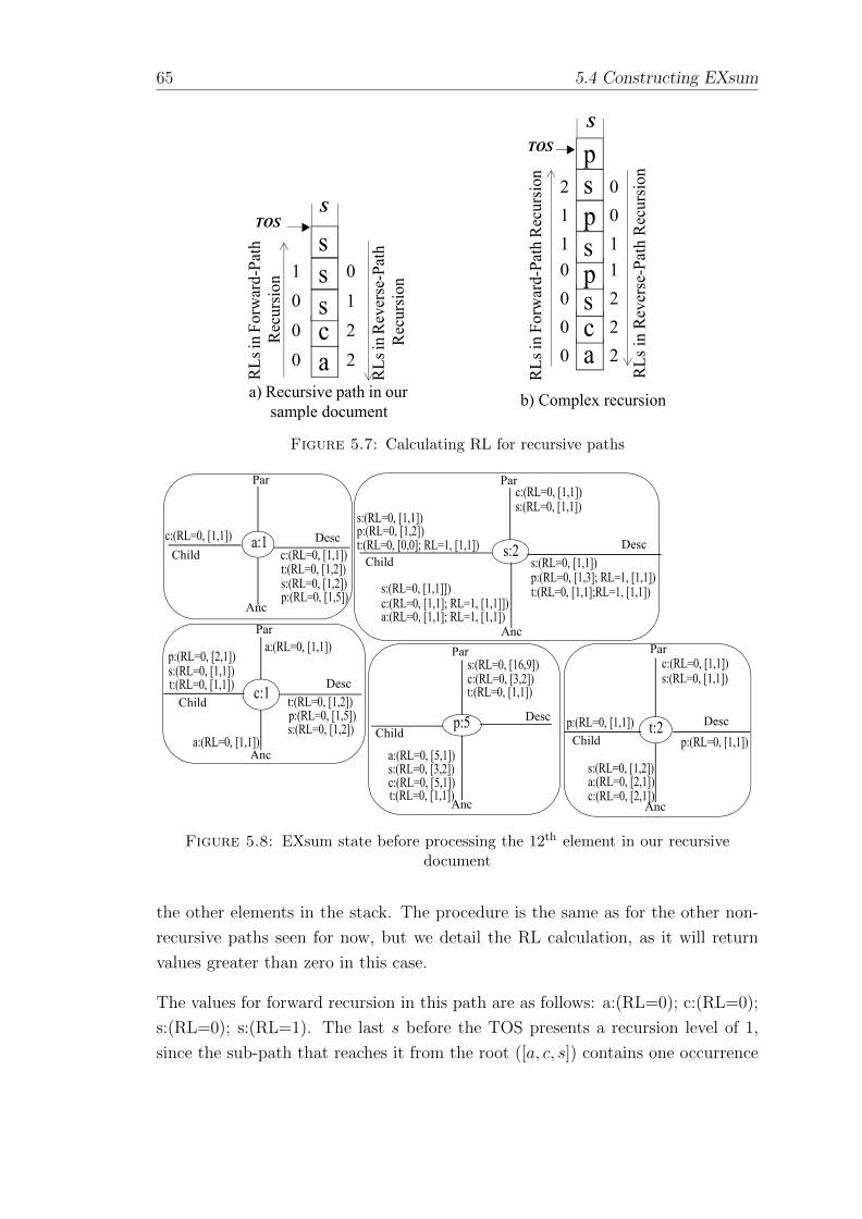
65 5.4 Constructing EXsum

a

TOS

csssS

RLs

in F

orw

ard-

Path

R

ecur

sion

RLs

in R

ever

se-P

ath

Rec

ursi

on

0001

a

TOS

csps

S

RLs

in F

orw

ard-

Path

Rec

ursi

on

RLs

in R

ever

se-P

ath

Rec

ursi

on

0000

2221

psp

112

100

2210

a) Recursive path in our sample document

b) Complex recursion

Figure 5.7: Calculating RL for recursive paths

s:2

Anc

Par

ChildDesct:(RL=0, [0,0]; RL=1, [1,1])

c:(RL=0, [1,1]; RL=1, [1,1]])a:(RL=0, [1,1]; RL=1, [1,1])

c:(RL=0, [1,1])

t:2

Anc

Par

ChildDesc

c:(RL=0, [2,1])

c:(RL=0, [1,1])

c:1

Anc

Par

ChildDesct:(RL=0, [1,1])

p:(RL=0, [2,1])s:(RL=0, [1,1])

a:(RL=0, [1,1])

p:(RL=0, [1,5])s:(RL=0, [1,2])

t:(RL=0, [1,2])p:5

Anc

Par

ChildDesc

a:(RL=0, [5,1])s:(RL=0, [3,2])c:(RL=0, [5,1])

s:(RL=0, [16,9])c:(RL=0, [3,2])

a:(RL=0, [2,1])

a:1

Anc

Par

ChildDesc

t:(RL=0, [1,2])s:(RL=0, [1,2])p:(RL=0, [1,5])

c:(RL=0, [1,1])

t:(RL=0, [1,1])

s:(RL=0, [1,1])

p:(RL=0, [1,1])

c:(RL=0, [1,1])

a:(RL=0, [1,1])

s:(RL=0, [1,1])

s:(RL=0, [1,2])

p:(RL=0, [1,1])

t:(RL=0, [1,1])

s:(RL=0, [1,1])

p:(RL=0, [1,2])s:(RL=0, [1,1])

s:(RL=0, [1,1]])p:(RL=0, [1,3]; RL=1, [1,1])t:(RL=0, [1,1];RL=1, [1,1])

Figure 5.8: EXsum state before processing the 12th element in our recursivedocument

the other elements in the stack. The procedure is the same as for the other non-

recursive paths seen for now, but we detail the RL calculation, as it will return

values greater than zero in this case.

The values for forward recursion in this path are as follows: a:(RL=0); c:(RL=0);

s:(RL=0); s:(RL=1). The last s before the TOS presents a recursion level of 1,

since the sub-path that reaches it from the root ([a, c, s]) contains one occurrence

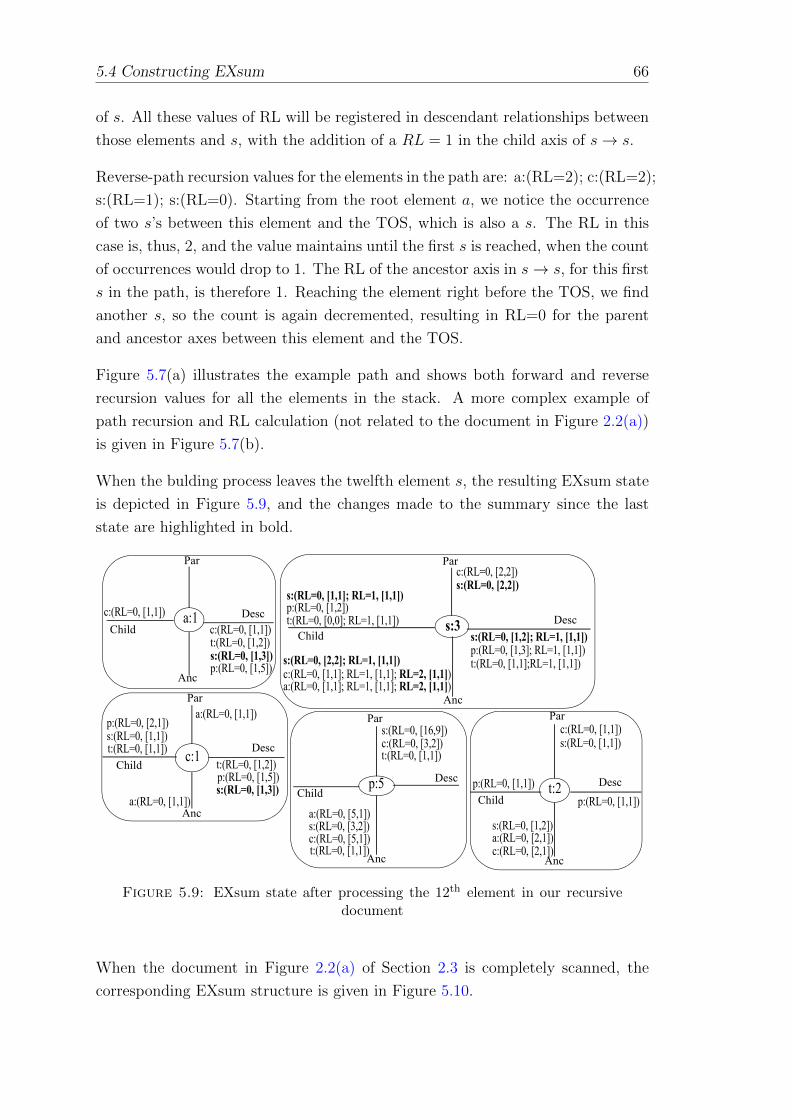
5.4 Constructing EXsum 66

of s. All these values of RL will be registered in descendant relationships between

those elements and s, with the addition of a RL = 1 in the child axis of s→ s.

Reverse-path recursion values for the elements in the path are: a:(RL=2); c:(RL=2);

s:(RL=1); s:(RL=0). Starting from the root element a, we notice the occurrence

of two s’s between this element and the TOS, which is also a s. The RL in this

case is, thus, 2, and the value maintains until the first s is reached, when the count

of occurrences would drop to 1. The RL of the ancestor axis in s→ s, for this first

s in the path, is therefore 1. Reaching the element right before the TOS, we find

another s, so the count is again decremented, resulting in RL=0 for the parent

and ancestor axes between this element and the TOS.

Figure 5.7(a) illustrates the example path and shows both forward and reverse

recursion values for all the elements in the stack. A more complex example of

path recursion and RL calculation (not related to the document in Figure 2.2(a))

is given in Figure 5.7(b).

When the bulding process leaves the twelfth element s, the resulting EXsum state

is depicted in Figure 5.9, and the changes made to the summary since the last

state are highlighted in bold.

s:3

Anc

Par

ChildDesct:(RL=0, [0,0]; RL=1, [1,1])

c:(RL=0, [1,1]; RL=1, [1,1]; RL=2, [1,1])a:(RL=0, [1,1]; RL=1, [1,1]; RL=2, [1,1])

c:(RL=0, [2,2])

t:2

Anc

Par

ChildDesc

c:(RL=0, [2,1])

c:(RL=0, [1,1])

c:1

Anc

Par

ChildDesct:(RL=0, [1,1])

p:(RL=0, [2,1])s:(RL=0, [1,1])

a:(RL=0, [1,1])

p:(RL=0, [1,5])s:(RL=0, [1,3])

t:(RL=0, [1,2])p:5

Anc

Par

ChildDesc

a:(RL=0, [5,1])s:(RL=0, [3,2])c:(RL=0, [5,1])

s:(RL=0, [16,9])c:(RL=0, [3,2])

a:(RL=0, [2,1])

a:1

Anc

Par

ChildDesc

t:(RL=0, [1,2])s:(RL=0, [1,3])p:(RL=0, [1,5])

c:(RL=0, [1,1])

t:(RL=0, [1,1])

s:(RL=0, [1,2]; RL=1, [1,1])

p:(RL=0, [1,1])

c:(RL=0, [1,1])

a:(RL=0, [1,1])

s:(RL=0, [1,1])

s:(RL=0, [1,2])

p:(RL=0, [1,1])

t:(RL=0, [1,1])

s:(RL=0, [2,2])

p:(RL=0, [1,2])s:(RL=0, [1,1]; RL=1, [1,1])

s:(RL=0, [2,2]; RL=1, [1,1])p:(RL=0, [1,3]; RL=1, [1,1])t:(RL=0, [1,1];RL=1, [1,1])

Figure 5.9: EXsum state after processing the 12th element in our recursivedocument

When the document in Figure 2.2(a) of Section 2.3 is completely scanned, the

corresponding EXsum structure is given in Figure 5.10.

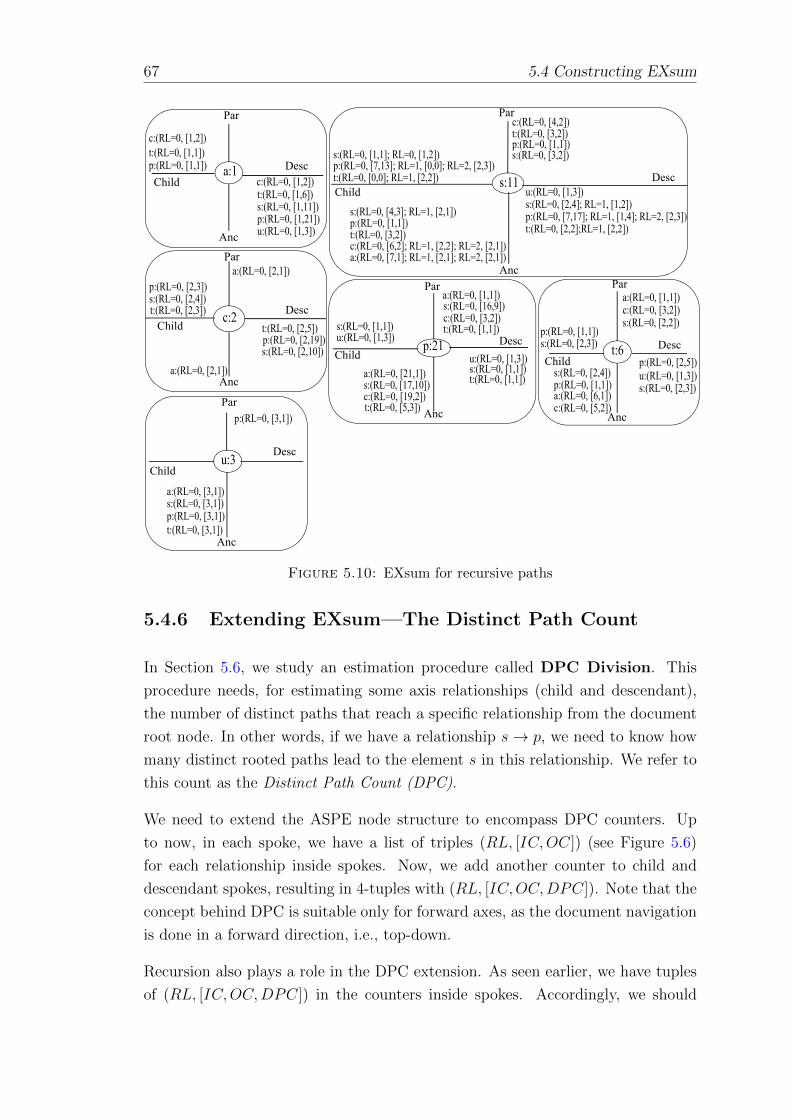
67 5.4 Constructing EXsum

s:11

Anc

Par

ChildDesct:(RL=0, [0,0]; RL=1, [2,2])

u:(RL=0, [1,3])

t:(RL=0, [3,2])c:(RL=0, [6,2]; RL=1, [2,2]; RL=2, [2,1])a:(RL=0, [7,1]; RL=1, [2,1]; RL=2, [2,1])

c:(RL=0, [4,2])

t:6

Anc

Par

ChildDesc

c:(RL=0, [5,2])

c:(RL=0, [3,2])c:2

Anc

Par

ChildDesct:(RL=0, [2,3])

p:(RL=0, [2,3])s:(RL=0, [2,4])

a:(RL=0, [2,1])

p:(RL=0, [2,19])s:(RL=0, [2,10])

t:(RL=0, [2,5])p:21

Anc

Par

ChildDesc

a:(RL=0, [21,1])s:(RL=0, [17,10])c:(RL=0, [19,2])

s:(RL=0, [16,9])c:(RL=0, [3,2])

a:(RL=0, [6,1])

u:(RL=0, [1,3])

u:(RL=0, [1,3])

a:1

Anc

Par

ChildDesc

t:(RL=0, [1,6])s:(RL=0, [1,11])p:(RL=0, [1,21])

p:(RL=0, [1,1])t:(RL=0, [1,1])c:(RL=0, [1,2])

u:3

Anc

Par

Child

Desc

a:(RL=0, [3,1])

p:(RL=0, [3,1])

t:(RL=0, [3,1])

s:(RL=0, [3,1])

a:(RL=0, [1,1])

s:(RL=0, [2,3])

a:(RL=0, [1,1])

t:(RL=0, [5,3])

u:(RL=0, [1,3])

s:(RL=0, [2,4]; RL=1, [1,2])

u:(RL=0, [1,3])p:(RL=0, [2,5])

t:(RL=0, [3,2])

p:(RL=0, [3,1])

c:(RL=0, [1,2])

a:(RL=0, [2,1])s:(RL=0, [2,3])

s:(RL=0, [2,2])

p:(RL=0, [1,1])s:(RL=0, [2,4])

p:(RL=0, [1,1])s:(RL=0, [1,1])

s:(RL=0, [1,1])t:(RL=0, [1,1])

t:(RL=0, [1,1])

p:(RL=0, [1,1])s:(RL=0, [3,2])

p:(RL=0, [7,13]; RL=1, [0,0]; RL=2, [2,3])s:(RL=0, [1,1]; RL=0, [1,2])

s:(RL=0, [4,3]; RL=1, [2,1])p:(RL=0, [1,1]) p:(RL=0, [7,17]; RL=1, [1,4]; RL=2, [2,3])

t:(RL=0, [2,2];RL=1, [2,2])

Figure 5.10: EXsum for recursive paths

5.4.6 Extending EXsum—The Distinct Path Count

In Section 5.6, we study an estimation procedure called DPC Division. This

procedure needs, for estimating some axis relationships (child and descendant),

the number of distinct paths that reach a specific relationship from the document

root node. In other words, if we have a relationship s→ p, we need to know how

many distinct rooted paths lead to the element s in this relationship. We refer to

this count as the Distinct Path Count (DPC).

We need to extend the ASPE node structure to encompass DPC counters. Up

to now, in each spoke, we have a list of triples (RL, [IC,OC]) (see Figure 5.6)

for each relationship inside spokes. Now, we add another counter to child and

descendant spokes, resulting in 4-tuples with (RL, [IC,OC,DPC]). Note that the

concept behind DPC is suitable only for forward axes, as the document navigation

is done in a forward direction, i.e., top-down.

Recursion also plays a role in the DPC extension. As seen earlier, we have tuples

of (RL, [IC,OC,DPC]) in the counters inside spokes. Accordingly, we should

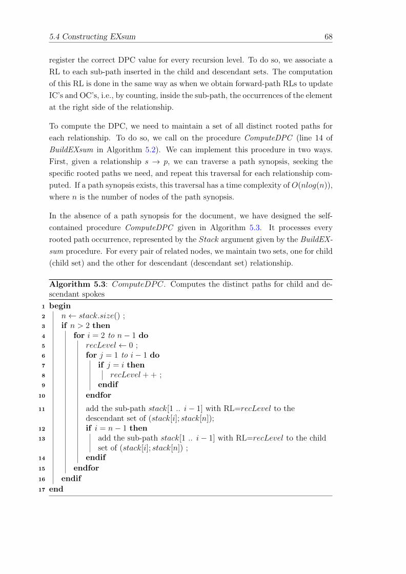
5.4 Constructing EXsum 68

register the correct DPC value for every recursion level. To do so, we associate a

RL to each sub-path inserted in the child and descendant sets. The computation

of this RL is done in the same way as when we obtain forward-path RLs to update

IC’s and OC’s, i.e., by counting, inside the sub-path, the occurrences of the element

at the right side of the relationship.

To compute the DPC, we need to maintain a set of all distinct rooted paths for

each relationship. To do so, we call on the procedure ComputeDPC (line 14 of

BuildEXsum in Algorithm 5.2). We can implement this procedure in two ways.

First, given a relationship s → p, we can traverse a path synopsis, seeking the

specific rooted paths we need, and repeat this traversal for each relationship com-

puted. If a path synopsis exists, this traversal has a time complexity of O(nlog(n)),

where n is the number of nodes of the path synopsis.

In the absence of a path synopsis for the document, we have designed the self-

contained procedure ComputeDPC given in Algorithm 5.3. It processes every

rooted path occurrence, represented by the Stack argument given by the BuildEX-

sum procedure. For every pair of related nodes, we maintain two sets, one for child

(child set) and the other for descendant (descendant set) relationship.

Algorithm 5.3: ComputeDPC. Computes the distinct paths for child and de-scendant spokes

begin1

n← stack.size() ;2

if n > 2 then3

for i = 2 to n− 1 do4

recLevel← 0 ;5

for j = 1 to i− 1 do6

if j = i then7

recLevel + + ;8

endif9

endfor10

add the sub-path stack[1 .. i− 1] with RL=recLevel to the11

descendant set of (stack[i]; stack[n]);if i = n− 1 then12

add the sub-path stack[1 .. i− 1] with RL=recLevel to the child13

set of (stack[i]; stack[n]) ;endif14

endfor15

endif16

end17

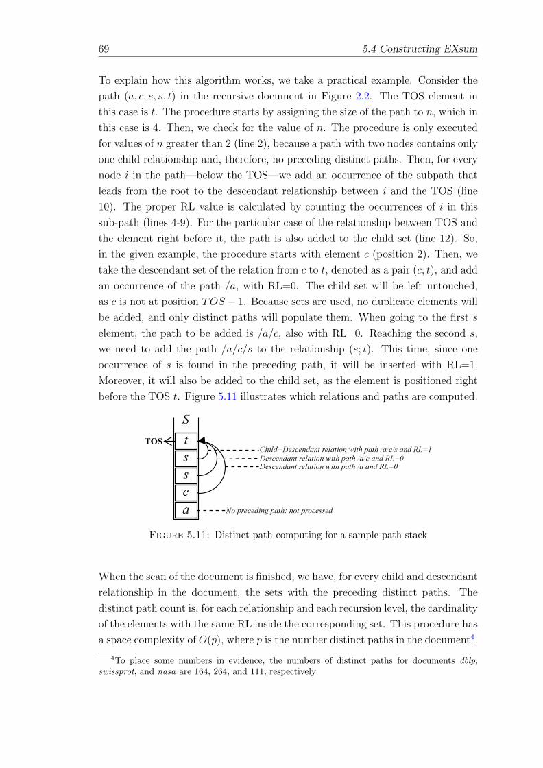
69 5.4 Constructing EXsum

To explain how this algorithm works, we take a practical example. Consider the

path (a, c, s, s, t) in the recursive document in Figure 2.2. The TOS element in

this case is t. The procedure starts by assigning the size of the path to n, which in

this case is 4. Then, we check for the value of n. The procedure is only executed

for values of n greater than 2 (line 2), because a path with two nodes contains only

one child relationship and, therefore, no preceding distinct paths. Then, for every

node i in the path—below the TOS—we add an occurrence of the subpath that

leads from the root to the descendant relationship between i and the TOS (line

10). The proper RL value is calculated by counting the occurrences of i in this

sub-path (lines 4-9). For the particular case of the relationship between TOS and

the element right before it, the path is also added to the child set (line 12). So,

in the given example, the procedure starts with element c (position 2). Then, we

take the descendant set of the relation from c to t, denoted as a pair (c; t), and add

an occurrence of the path /a, with RL=0. The child set will be left untouched,

as c is not at position TOS − 1. Because sets are used, no duplicate elements will

be added, and only distinct paths will populate them. When going to the first s

element, the path to be added is /a/c, also with RL=0. Reaching the second s,

we need to add the path /a/c/s to the relationship (s; t). This time, since one

occurrence of s is found in the preceding path, it will be inserted with RL=1.

Moreover, it will also be added to the child set, as the element is positioned right

before the TOS t. Figure 5.11 illustrates which relations and paths are computed.

Figure 5.11: Distinct path computing for a sample path stack

When the scan of the document is finished, we have, for every child and descendant

relationship in the document, the sets with the preceding distinct paths. The

distinct path count is, for each relationship and each recursion level, the cardinality

of the elements with the same RL inside the corresponding set. This procedure has

a space complexity of O(p), where p is the number distinct paths in the document4.

4To place some numbers in evidence, the numbers of distinct paths for documents dblp,swissprot, and nasa are 164, 264, and 111, respectively

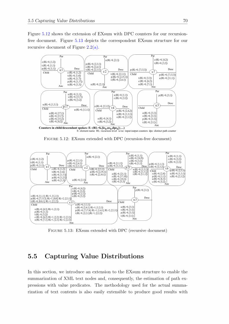
5.5 Capturing Value Distributions 70

Figure 5.12 shows the extension of EXsum with DPC counters for our recursion-

free document. Figure 5.13 depicts the correspondent EXsum structure for our

recursive document of Figure 2.2(a).

s:7

Anc

Par

Child

Descp:(RL=0, [7,13,3])

p:(RL=0, [7,13,3])t:(RL=0, [3,3])c:(RL=0, [6,2])a:(RL=0, [7,1])

c:(RL=0, [4,2])

t:4

Anc

Par

ChildDesc

c:(RL=0, [3,2])

c:(RL=0, [3,2])

c:2

Anc

Par

ChildDesct:(RL=0, [2,3,1])

p:(RL=0, [2,3,1])s:(RL=0, [2,4,1])

a:(RL=0, [2,1])

p:(RL=0, [2,15,1])s:(RL=0, [2,6,1])

t:(RL=0, [2,3,1])

p:17

Anc

Par

ChildDesc

a:(RL=0, [17,1])s:(RL=0, [13,7])c:(RL=0, [15,2])

s:(RL=0, [13,7])c:(RL=0, [3,2])

a:(RL=0, [4,1])

u:(RL=0, [1,3,1])

u:(RL=0, [1,3,1])

a:1

Anc

Par

ChildDesc

t:(RL=0, [1,4])s:(RL=0, [1,7])p:(RL=0, [1,17])

p:(RL=0, [1,1])t:(RL=0, [1,1])c:(RL=0, [1,2])

u:3

Anc

Par

Child

Desc

a:(RL=0, [3,1])

p:(RL=0, [3,1])

t:(RL=0, [3,1])

s:(RL=0, [3,1])

a:(RL=0, [1,1])

s:(RL=0, [2,3,2])

a:(RL=0, [1,1])

t:(RL=0, [4,2])

u:(RL=0, [1,3])

u:(RL=0, [3,1,1])

u:(RL=0, [1,3,1])p:(RL=0, [2,4,2])

t:(RL=0, [3,2])

p:(RL=0, [3,1])

c:(RL=0, [1,2])

a:(RL=0, [2,1])

s:(RL=0, [2,3,2])

Counters in child/descendant spokes: E: (RL=k,[ick,ock,dpck];…)E: element name RL: recursion level ic/oc: input/output counters dpc: distinct path counter

Figure 5.12: EXsum extended with DPC (recursion-free document)

s:11

Anc

Par

ChildDesct:(RL=0, [0,0,1]; RL=1, [2,2,2])

u:(RL=0, [1,3,1])

t:(RL=0, [3,2])c:(RL=0, [6,2]; RL=1, [2,2]; RL=2, [2,1])a:(RL=0, [7,1]; RL=1, [2,1]; RL=2, [2,1])

c:(RL=0, [4,2])

t:6

Anc

Par

ChildDesc

c:(RL=0, [5,2])

c:(RL=0, [3,2])

c:2

Anc

Par

ChildDesct:(RL=0, [2,3,1])

p:(RL=0, [2,3,1])s:(RL=0, [2,4,1])

a:(RL=0, [2,1])

p:(RL=0, [2,19,1])s:(RL=0, [2,10,1])

t:(RL=0, [2,5,1]) p:21

Anc

Par

ChildDesc

a:(RL=0, [21,1])s:(RL=0, [17,10])c:(RL=0, [19,2])

s:(RL=0, [16,9])c:(RL=0, [3,2])

a:(RL=0, [6,1])

u:(RL=0, [1,3,1])u:(RL=0, [1,3,1])

a:1

Anc

Par

ChildDesc

t:(RL=0, [1,6])s:(RL=0, [1,11])p:(RL=0, [1,21])

p:(RL=0, [1,1])t:(RL=0, [1,1])c:(RL=0, [1,2])

u:3

Anc

Par

Child

Desc

a:(RL=0, [3,1])

p:(RL=0, [3,1])

t:(RL=0, [3,1])

s:(RL=0, [3,1])

a:(RL=0, [1,1])

s:(RL=0, [2,3,2])

a:(RL=0, [1,1])

t:(RL=0, [5,3])u:(RL=0, [1,3])

s:(RL=0, [2,4,1]; RL=1, [1,2,1])

u:(RL=0, [1,3,1])p:(RL=0, [2,5,3])

t:(RL=0, [3,2])

p:(RL=0, [3,1])

c:(RL=0, [1,2])

a:(RL=0, [2,1])s:(RL=0, [2,3,2])

s:(RL=0, [2,2])

p:(RL=0, [1,1])s:(RL=0, [2,4])

p:(RL=0, [1,1,1])s:(RL=0, [1,1,1])

s:(RL=0, [1,11,])t:(RL=0, [1,1,1])

t:(RL=0, [1,1])

p:(RL=0, [1,1])s:(RL=0, [3,2])

p:(RL=0, [7,13,3]; RL=1, [0,0]; RL=2, [2,3,1])s:(RL=0, [1,1,1]; RL=1, [1,2,1])

s:(RL=0, [4,3]; RL=1, [2,1])p:(RL=0, [1,1]) p:(RL=0, [7,17,4]; RL=1, [1,4,1]; RL=2, [2,3,1])

t:(RL=0, [2,2,1];RL=1, [2,2,2])

Figure 5.13: EXsum extended with DPC (recursive document)

5.5 Capturing Value Distributions

In this section, we introduce an extension to the EXsum structure to enable the

summarization of XML text nodes and, consequently, the estimation of path ex-

pressions with value predicates. The methodology used for the actual summa-

rization of text contents is also easily extensible to produce good results with

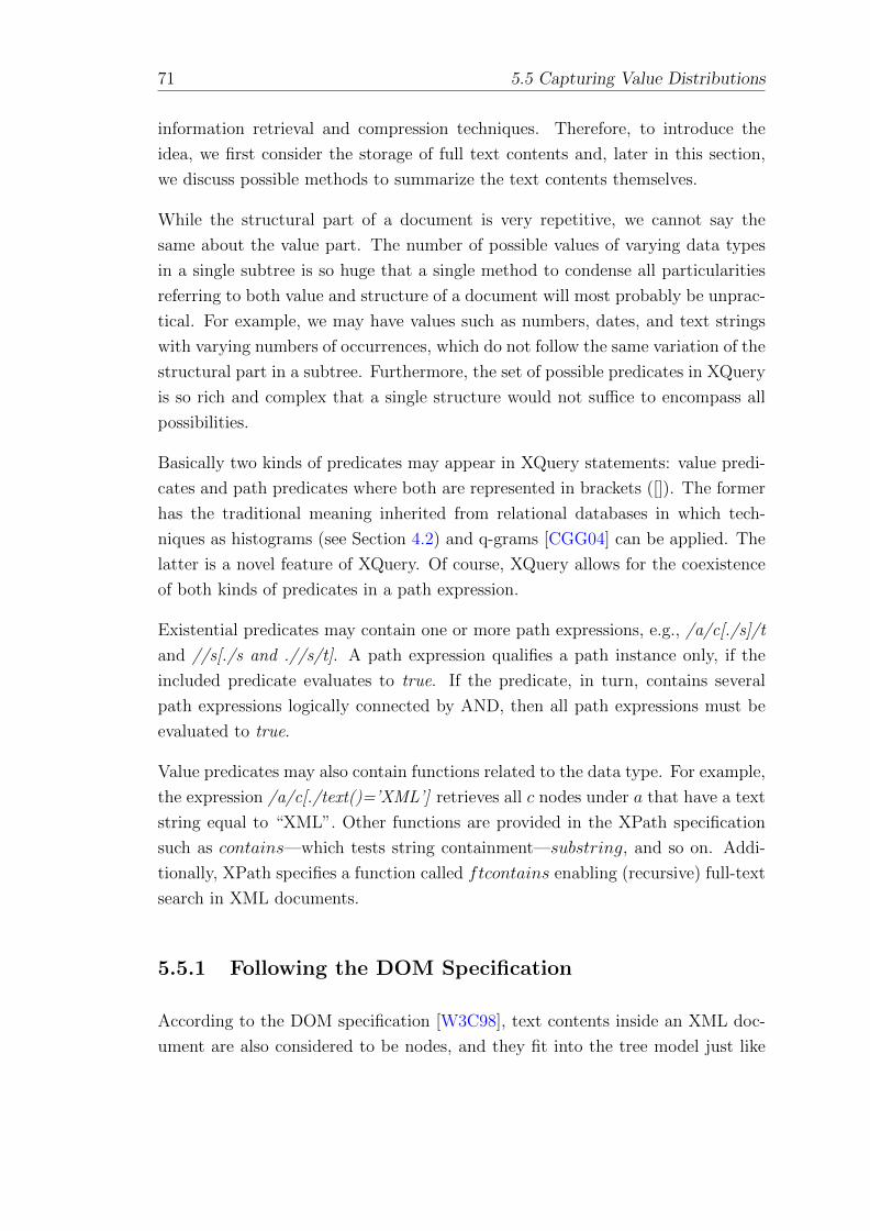
71 5.5 Capturing Value Distributions

information retrieval and compression techniques. Therefore, to introduce the

idea, we first consider the storage of full text contents and, later in this section,

we discuss possible methods to summarize the text contents themselves.

While the structural part of a document is very repetitive, we cannot say the

same about the value part. The number of possible values of varying data types

in a single subtree is so huge that a single method to condense all particularities

referring to both value and structure of a document will most probably be unprac-

tical. For example, we may have values such as numbers, dates, and text strings

with varying numbers of occurrences, which do not follow the same variation of the

structural part in a subtree. Furthermore, the set of possible predicates in XQuery

is so rich and complex that a single structure would not suffice to encompass all

possibilities.

Basically two kinds of predicates may appear in XQuery statements: value predi-

cates and path predicates where both are represented in brackets ([]). The former

has the traditional meaning inherited from relational databases in which tech-

niques as histograms (see Section 4.2) and q-grams [CGG04] can be applied. The

latter is a novel feature of XQuery. Of course, XQuery allows for the coexistence

of both kinds of predicates in a path expression.

Existential predicates may contain one or more path expressions, e.g., /a/c[./s]/t

and //s[./s and .//s/t]. A path expression qualifies a path instance only, if the

included predicate evaluates to true. If the predicate, in turn, contains several

path expressions logically connected by AND, then all path expressions must be

evaluated to true.

Value predicates may also contain functions related to the data type. For example,

the expression /a/c[./text()=’XML’] retrieves all c nodes under a that have a text

string equal to “XML”. Other functions are provided in the XPath specification

such as contains—which tests string containment—substring, and so on. Addi-

tionally, XPath specifies a function called ftcontains enabling (recursive) full-text

search in XML documents.

5.5.1 Following the DOM Specification

According to the DOM specification [W3C98], text contents inside an XML doc-

ument are also considered to be nodes, and they fit into the tree model just like

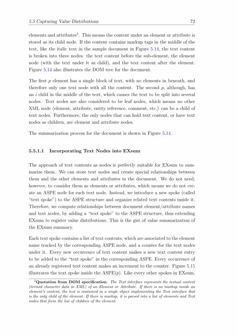
5.5 Capturing Value Distributions 72

elements and attributes5. This means the content under an element or attribute is

stored as its child node. If the content contains markup tags in the middle of the

text, like the italic text in the sample document in Figure 5.14, the text content

is broken into three nodes: the text content before the sub-element, the element

node (with the text under it as child), and the text content after the element.

Figure 5.14 also illustrates the DOM tree for the document.

The first p element has a single block of text, with no elements in beneath, and

therefore only one text node with all the content. The second p, although, has

an i child in the middle of the text, which causes the text to be split into several

nodes. Text nodes are also considered to be leaf nodes, which means no other

XML node (element, attribute, entity reference, comment, etc.) can be a child of

text nodes. Furthermore, the only nodes that can hold text content, or have text

nodes as children, are element and attribute nodes.

The summarization process for the document is shown in Figure 5.14.

5.5.1.1 Incorporating Text Nodes into EXsum

The approach of text contents as nodes is perfectly suitable for EXsum to sum-

marize them. We can store text nodes and create special relationships between

them and the other elements and attributes in the document. We do not need,

however, to consider them as elements or attributes, which means we do not cre-

ate an ASPE node for each text node. Instead, we introduce a new spoke (called

“text spoke”) to the ASPE structure and organize related text contents inside it.

Therefore, we compute relationships between document element/attribute names

and text nodes, by adding a “text spoke” to the ASPE structure, thus extending

EXsum to register value distributions. This is the gist of value summarization of

the EXsum summary.

Each text spoke contains a list of text contents, which are associated to the element

name tracked by the corresponding ASPE node, and a counter for the text nodes

under it. Every new occurrence of text content makes a new text content entry

to be added to the “text spoke” in the corresponding ASPE. Every occurrence of

an already registered text content makes an increment to the counter. Figure 5.15

illustrates the text spoke inside the ASPE(p). Like every other spokes in EXsum,

5Quotation from DOM specification. The Text interface represents the textual content(termed character data in XML) of an Element or Attribute. If there is no markup inside anelement’s content, the text is contained in a single object implementing the Text interface thatis the only child of the element. If there is markup, it is parsed into a list of elements and Textnodes that form the list of children of the element.

73 5.5 Capturing Value Distributions

html

body

h1 p p

iPage title This is the first text

content.Here is some text in , at the second para-

graph.

italic

XM

L do

cum

ent

DO

M tr

ee

Element

Text nodes

<html> <body> <h1> Page title </h1> <p> This is the first text content. </p> <p> Here is some text in <i>italic</i>, at the second paragraph. </p> </body></html>

Figure 5.14: Example of an XML document with text nodes and DOM tree

relationships are registered independent of the physical location of the element

occurrence, so all text under any p node is stored in the same spoke.

This approach is simple and straight-forward. However, it is not suitable for

summarization purposes, because text nodes represent most of the XML data in

many practical XML documents and the amount of space consumed by such an

approach can be very expensive and, therefore, not affordable for query estimation.

In the next section, we introduce some techniques to summarize and compress the

text contents inside text spokes.

5.5.2 EXsum’s Text Content Summarization Framework

In this section, we gradually introduce techniques to progressively improve the

summarization of text values by compressing or rearranging the information in

text spokes.

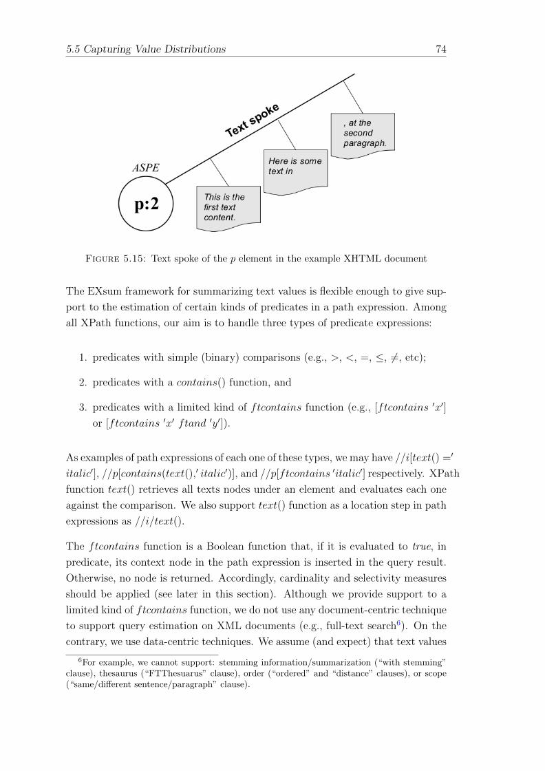
5.5 Capturing Value Distributions 74

Figure 5.15: Text spoke of the p element in the example XHTML document

The EXsum framework for summarizing text values is flexible enough to give sup-

port to the estimation of certain kinds of predicates in a path expression. Among

all XPath functions, our aim is to handle three types of predicate expressions:

1. predicates with simple (binary) comparisons (e.g., >, <, =, ≤, 6=, etc);

2. predicates with a contains() function, and

3. predicates with a limited kind of ftcontains function (e.g., [ftcontains ′x′]

or [ftcontains ′x′ ftand ′y′]).

As examples of path expressions of each one of these types, we may have //i[text() =′

italic′], //p[contains(text(),′ italic′)], and //p[ftcontains ′italic′] respectively. XPath

function text() retrieves all texts nodes under an element and evaluates each one

against the comparison. We also support text() function as a location step in path

expressions as //i/text().

The ftcontains function is a Boolean function that, if it is evaluated to true, in

predicate, its context node in the path expression is inserted in the query result.

Otherwise, no node is returned. Accordingly, cardinality and selectivity measures

should be applied (see later in this section). Although we provide support to a

limited kind of ftcontains function, we do not use any document-centric technique

to support query estimation on XML documents (e.g., full-text search6). On the

contrary, we use data-centric techniques. We assume (and expect) that text values

6For example, we cannot support: stemming information/summarization (“with stemming”clause), thesaurus (“FTThesuarus” clause), order (“ordered” and “distance” clauses), or scope(“same/different sentence/paragraph” clause).

75 5.5 Capturing Value Distributions

in documents are short —at most, not so long as a half page of text—and in most

of cases consisting of numerical values and nouns.

We do not claim that we present one summarization technique that is suitable

for all kinds of predicates studied. Instead, the framework is able to construct

any necessary structure (or set of structures), balancing compression and loss of

information, to support predicates types. The novelty here is, however, the esti-

mation method relating cardinality estimations of text values with the structural

part of a path expression, which yields estimated measures on the cardinality of

path expression and predicate selectivity.

5.5.2.1 The Issue of Data Type

As a common step to improve our text summary, we should consider the identifica-

tion of data types in text spokes. XML schema [W3C08] provides an explicit data

type information for values under an element/attribute. If we have XML schema,

we derive data type information for each text spoke in ASPE nodes and drive the

suitable compression technique. In the absence of schema information, we assume

the existence of two functions: isNumber() and isString(), which, applied to the

values of a text spoke, give us the corresponding basic data type, whether numeric

or not.

Different data types require different summarization methods. For example, his-

tograms are useful for numeric data, whereas q-grams are suitable for text strings.

Therefore, we do not claim to propose a general solution for all possible data

types. Rather, we build a framework in which one can use the most suitable

summarization method(s) to answer a given query workload, in a tailored way.

5.5.2.2 The Three-step Summarization

We now present a three-step summarization process which one can follow com-

pletely or partially. The result of each step is consistent, in the sense that an

implementation can go only to a specific step, apply the summarization tech-

nique(s) suitable for the step, and then not go further to other steps at all. It is

the responsibility of the system administrator to configure the EXsum framework

to compute the necessary summarization structure(s).

Our value summarization framework is a compound of three phases. The first

phase collects all the values under a specific element/attribute name applying

5.5 Capturing Value Distributions 76

the respective data type functions and creating the so-called frequency vector.

The frequency vector captures for each distinct value the corresponding number

of occurrences (frequency). The second phase is optional and normally applied

to strings. In this phase, the strings are tokenized where a token can mean a

q-gram, a word, or any substring of arbitrary length. The tokenization is thus

implementation-dependent. One can tailor the building of tokens according to an

expected query workload. For example, if it is known that most queries search

words in an XML document, tokens can be constructed accordingly, i.e., a token is

any set of characters between two blank spaces. The third phase applies a suitable

compression technique. For example, for numeric data, we can apply histograms.

Step 1: Create Frequency Vectors. The first enhancement is to eliminate

repeated occurrences of the same text under an ASPE spoke by creating frequency

vectors. This is considered to be the basic step towards a good summarization

methodology. In this approach, instead of maintaining a plain list of text contents,

we would have a vector with one entry for each distinct text occurrence and the

number of occurrences (frequency) of the associated text set. In this case, every

time a text is being added to the summary, we must first see if it is already

present inside the desired spoke and, in the affirmative case, simply increment the

associated counter. Otherwise, a new entry containing the text would be added

to the vector.

Frequency vectors are useful to support any predicates handled by EXsum. De-

spite that, this technique itself does not provide a significant summarization im-

provement, since repeated occurrences of full text contents are somewhat rare in

the majority of practical XML documents. The exception are element content or

attribute values with a restricted domain, like the boolean set (true or false) or

values inside an enumeration (e.g., male, female). In other words, the frequency

vector may be large.

However, we can gather at least two summary information from frequency vectors.

To favor storage space to accommodate the summary, we can strip (and store for

the spoke) only the number of entries in the vector (i.e., the number of distinct

values) and the total frequency (i.e., sum of frequencies). Assuming uniform dis-

tribution in text values, these two pieces of information can support the estimation

of predicate types 1 and 3. In fact, this information is always captured in addition

to the application of any compression technique. The reason behind this is to

support queries involving text() function in path expressions (as a location step).

Another compression technique is to store the n most frequent entries in the vector

and make the uniform distribution assumption for the rest (storing, for that part,

77 5.5 Capturing Value Distributions

only the number of distinct values and the total frequency). In this case, value n

is determined by a tuning parameter.

Another possible task in this step is to make a statistical study on the frequency

vector to obtain statistical measures such as variance, standard deviation, mean,

and skewness. This information can drive the application of suitable compression

techniques in Step 3, thus making them a parametric technique7.

Step 2: Break into Tokens. Since occurrences of full text blocks tend to be

unique inside a general XML document, we try to break the blocks of text in less

representative information, having, therefore, a more restricted set of values. The

natural way of doing that in text blocks is by splitting into tokens. Although the

meaning of token varies a lot (it has several possible definitions), let us assume, for

a better discussion, that a token corresponds to a word (i.e., a termed sequence

of characters between two blank spaces in the text). When we take many text

occurrences and break them into token occurrences, the amount of repeated values

raises significantly. When creating frequency vectors over a set of tokens, we have,

therefore, a much more compact structure, since repeated occurrences can be

eliminated.

While providing an efficient compression of data, this method (token-based fre-

quency vector) introduces a big loss of information, since the composition of words

to form the text data is lost, and the resulting data looses much of its significance.

In Figure 5.16, we illustrate the result of applying token-based frequency vectors

(word splitting) to the ASPE node of p in Figure 5.15. Due to this loss, we cannot

estimate type 1 predicates.

However, by applying compression techniques such as histograms or q-grams on

the token-based vector, we can approximate estimations for predicate types 2 and

3. How good or bad the estimation results are with such techniques is an issue

which should be empirically evaluated. In any case, if storage space is a concern,

we can also apply techniques pointed out in Step 1 using the uniform distribution

assumption for estimation.

Step 3: Apply Compression Methods. Whatever frequency vector we have,

we can always apply compression techniques. The support of a predicate type de-

pends on the frequency vector type (text-based or token-based). The application of

7Parametric statistical techniques depend on a prior knowledge of the distribution of a set tobe applied. Non-parametric techniques are applied ignoring such a distribution. For example,histograms can be considered a non-parametric technique.

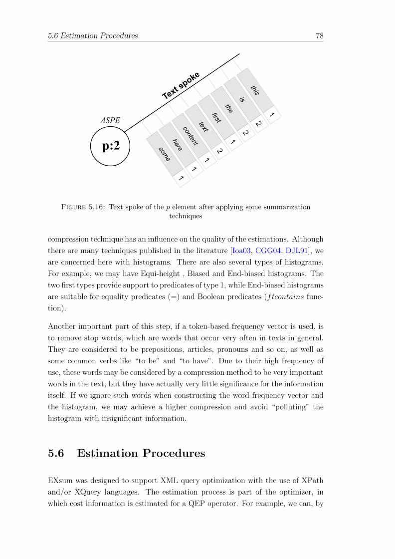
5.6 Estimation Procedures 78

p:2

ASPE

Text spoke

this

1

is

2

the

2

first

1

text

2

content

1

here

1

some

1Figure 5.16: Text spoke of the p element after applying some summarization

techniques

compression technique has an influence on the quality of the estimations. Although

there are many techniques published in the literature [Ioa03, CGG04, DJL91], we

are concerned here with histograms. There are also several types of histograms.

For example, we may have Equi-height , Biased and End-biased histograms. The

two first types provide support to predicates of type 1, while End-biased histograms

are suitable for equality predicates (=) and Boolean predicates (ftcontains func-

tion).

Another important part of this step, if a token-based frequency vector is used, is

to remove stop words, which are words that occur very often in texts in general.

They are considered to be prepositions, articles, pronouns and so on, as well as

some common verbs like “to be” and “to have”. Due to their high frequency of

use, these words may be considered by a compression method to be very important

words in the text, but they have actually very little significance for the information

itself. If we ignore such words when constructing the word frequency vector and

the histogram, we may achieve a higher compression and avoid “polluting” the

histogram with insignificant information.

5.6 Estimation Procedures

EXsum was designed to support XML query optimization with the use of XPath

and/or XQuery languages. The estimation process is part of the optimizer, in

which cost information is estimated for a QEP operator. For example, we can, by

79 5.6 Estimation Procedures

using EXsum, estimate the cost of Structural Join (STJ) [AKJP+02] or Holistic

Twig Join (HTJ) [BKS02] operators in a query plan. Obviously, we are aware

that a cost model is also necessary [WH09] in order to calculate the total cost of

a QEP. We are not, however, concerned with the cost model, but with estimation

mechanism and procedures provided by EXsum, which can be used in a full XML

query optimizer process.

Basically, two kinds of information can be estimated with EXsum: path cardinality

and path selectivity. The former corresponds to the number of document nodes

resulting from the processing of a path expression. These nodes are given back to

the user as result, with their respective subtrees. The latter comes to play when

predicates are present in path expressions and it is also used in the cost model of

an optimizer. We study both in this section, by using path expressions which are

the base for the two main XML query languages.

As studied in Section 2.2.1, a path expression has three components. For example,

a path expression such as /x/y//z has three steps: /x, /y and //z. For each step,

context nodes are “document root”, x, and y, respectively. Axes are child (/) and

descendant(//). Node tests are respectively: x, y and z. The final result reveals

the number of z nodes in the document satisfying this expression. Such a path

expression can be operated by QEPs with a set of STJ operators, which directly

mirrors the semantic of the expression itself, or with a QEP with one (or more)

HTJ operators, which allows a “multi-way” join. The scope of this thesis abstracts

the differences between QEP approaches, and we focus only on the information

that can be provided to generate such plans.

5.6.1 Underlying Mechanism of EXsum’s Estimation

The EXsum estimation mechanism of a path expression is executed step by step.

It follows each location step in an expression, probes the ASPE node related to

the context node, inspects the spoke related to the axis, and accesses the node

test in the spoke, obtaining the cardinality estimation from the OC counter for

the step (occ). This makes the EXsum estimation process heavily step-based, and

understanding the process of a single step estimation is the key when figuring out

how it deals with full path expressions.

The mechanism takes the three step components as arguments and returns the

estimated cardinality of the node test in the result. To help in this process, we

introduce auxiliary information, which can be considered as the set of all “outside”

5.6 Estimation Procedures 80

information needed by the step estimation. This information may include recursion

levels, path descriptions, and instructions for the estimation mechanism.

To understand the general estimation process, we take the example document tree

given in Figure 2.1(c), as well as its correspondent EXsum sketch in Figure 5.5,

and detail the estimation of an example query: /a/c//s. Since the first location

step has a simple child axis and a is the root of the document, we access ASPE(a)

and return occ(/a) which is obtained directly from the number of occurrences of

a. In this case, the value of 1 is returned as the cardinality of this step. Then, for

the next step /c, we probe the child spoke of ASPE(a) for a c and find in its OC

counter a value of 2 (occ(/c)=2), which is the cardinality for this step. Finally, we

estimate the step //s. We proceed to ASPE(c) and probe its descendant spoke for

an s. At this point, we get occ(//s)=7 from the OC counter of s and the process

returns 7 as the cardinality of the path expression.

Note that, when a location step is estimated, its related ASPE node (and only

such ASPE node) has to be loaded into memory. This feature considerably reduces

the EXsum’s memory footprint to estimate path expressions. In fact, in the worst

case, the number of ASPE nodes to be loaded into memory is bounded by the

number of location steps in the expression. In other words, we do not need to

load the entire EXsum structure into memory to estimate a simple location step

or even multiple-step expressions. This feature is kept for all estimation cases,

whether on recursion-free or recursive path expressions.

Although a generic mechanism exists, many specific situations have to be handled,

such as different characteristics of each axis, recursion levels, methods to improve

accuracy, and special occasions such as root and leaf nodes. Moreover, we have

to cope with cases in which EXsum delivers accurate cardinalities and cases in

which an approximation has to take place. We study these issues in the following

sections.

5.6.2 Cases with Guaranteed Accuracy and Special Cases

The construction principle of EXsum exactly covers two-step path expressions con-

taining child, descendant, parent, and ancestor axes. As an important property,

the element-centered summarization, therefore, delivers accurate cardinalities for

them, when the evaluation starts from the root or an unique element name.

81 5.6 Estimation Procedures

5.6.2.1 The Special Case of the First Step

The first step of an XPath expression generates a special condition in the step

estimation process, since in this case we do not have an explicit context node,

and all searches start from the root node. Therefore, only downward-oriented

axes (/and //) are possible. If //x is the first location step, then occ(x) directly

delivers the cardinality of //x, i.e., the number of document nodes having element

name x. The same information can be derived by accessing the ASPE of the root

element and retrieving the OC in the descendant spoke of x. Path expression /x

refers to the root element of a document. When accessing ASPE(x), we have to

check whether its parent spoke is empty or not. If a parent is found, occ(/x) is

necessarily 0, otherwise it must be 1. As an example evaluated on the document

of Figure 2.1(c), //p and /p deliver cardinalities 17 and 0, respectively. The other

types of axes hardly make sense with respect to the root node and can, therefore,

be neglected.

5.6.2.2 Unique Element Names

Another special case occurs when the end step of an arbitrary long path expression

refers to a unique element name z. No matter what axis references occur in

the path expression, we immediately inspect ASPE(z) and, after having verified

that the entire path expression matches the path synopsis (which means the path

actually exists), deliver occ(z) as the accurate cardinality information.

For example, /a/t/s/p/u, //s/p/u or //t//p/u can be evaluated in this way and

all deliver (see Figure 2.1) cardinality 3. Note that the existence of unique element

names, to be verified using the path synopsis, is most valuable for cardinality esti-

mation. When referenced in some of the intermediate location steps, it can be used

to begin the estimation in the middle starting with precise cardinality information.

Assume some subtrees containing the element name p are appended to the u nodes

in the document of Figure 2.1; then the estimation of //t//s//u//p would begin

at ASPE(u) and return (for this example) accurate cardinality information.

5.6.3 Methods to Improve Accuracy

EXsum delivers accurate cardinality results for all path expressions on homonym-

free documents and for path expressions with one and two location steps on

recursion-free document paths. We believe that these cases, where the EXsum

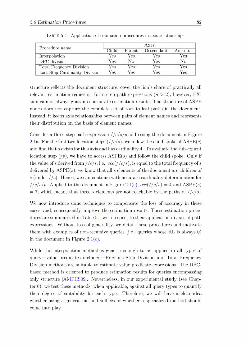
5.6 Estimation Procedures 82

Table 5.1: Application of estimation procedures in axis relationships.

Procedure nameAxes

Child Parent Descendant AncestorInterpolation Yes Yes Yes YesDPC division Yes No Yes NoTotal Frequency Division Yes Yes Yes YesLast Step Cardinality Division Yes Yes Yes Yes

structure reflects the document structure, cover the lion’s share of practically all

relevant estimation requests. For n-step path expressions (n > 2), however, EX-

sum cannot always guarantee accurate estimation results. The structure of ASPE

nodes does not capture the complete set of root-to-leaf paths in the document.

Instead, it keeps axis relationships between pairs of element names and represents

their distribution on the basis of element names.

Consider a three-step path expression //c/s/p addressing the document in Figure

2.1a. For the first two location steps (//c/s), we follow the child spoke of ASPE(c)

and find that s exists for this axis and has cardinality 4. To evaluate the subsequent

location step (/p), we have to access ASPE(s) and follow the child spoke. Only if

the value of s derived from //c/s, i.e., occ(//c/s), is equal to the total frequency of s

delivered by ASPE(s), we know that all s elements of the document are children of

c (under //c). Hence, we can continue with accurate cardinality determination for

//c/s/p. Applied to the document in Figure 2.1(c), occ(//c/s) = 4 and ASPE(s)

= 7, which means that three s elements are not reachable by the paths of //c/s.

We now introduce some techniques to compensate the loss of accuracy in these

cases, and, consequently, improve the estimation results. These estimation proce-

dures are summarized in Table 5.1 with respect to their application in axes of path

expressions. Without loss of generality, we detail these procedures and motivate

them with examples of non-recursive queries (i.e., queries whose RL is always 0)

in the document in Figure 2.1(c).

While the interpolation method is generic enough to be applied in all types of

query—value predicates included—Previous Step Division and Total Frequency

Division methods are suitable to estimate value predicate expressions. The DPC-

based method is oriented to produce estimation results for queries encompassing

only structure [AMFHS09]. Nevertheless, in our experimental study (see Chap-

ter 6), we test these methods, when applicable, against all query types to quantify

their degree of suitability for each type. Therefore, we will have a clear idea

whether using a generic method suffices or whether a specialized method should

come into play.

83 5.6 Estimation Procedures

5.6.3.1 Interpolation

In this estimation procedure, a path expression is decomposed into overlapping

two-location-step fractions and a linear interpolation takes place to combine their

results, assuming the uniform distribution of elements related to the “overlapped”

node tests of these fractions.

To evaluate a path expression //x/y//z, two overlapping two-location-step frac-

tions are considered: //x/y and y//z. For the partial expressions //x/y and

y//z, we access ASPE(x) and ASPE(y) (whose values are equivalent to occ(//x)

and occ(//y), respectively) and follow the ASPE spokes for the second location

steps to obtain occ(//x/y) and occ(//y//z). Because not all y nodes of //y//z

find a matching partner in the y nodes of //x/y, we assume uniform element dis-

tribution for the y nodes to enable a straightforward combination of estimates for

such partial expressions. By using the ratio C1/C2, we linearly interpolate the

number of occurrences of the subsequent step y//z to estimate occ(//x/y//z). In

this case, C1 is given by occ(//x/y) and C2 by the total frequency of the element

y; thus, C1 ≥ C2 always holds. The result of step estimation is then given by:

C1

C2× occ(y//z)

This interpolation could be applied step by step, such that we gain estimation

heuristics for n-step path expressions. If more accurate information is present

(e.g., by mining entire paths), it is used instead. Estimating occ(//c/s/p) from

the document in Figure 2.1a, we obtain C1 = 4 and C2 = 7, and the interpolated

cardinality C1/C2 ∗ (occ(s/p)) = 4/7 ∗ (13) (approx. 7.43), whereas the actual

cardinality for the path expression //c/s/p is 9.

5.6.3.2 DPC-based Estimation

The DPC-based estimation procedure relies on the assumption of uniform distri-

bution of document paths leading to a location step. The idea is to count in how

many different ways a node can be reached starting from the root node in the

document (see Section 5.4.6), and divide the occ(step) cardinality by this number.

When using recursion, these distinct paths are also classified according to their

recursion level.

Consider the path expression /a/c/s/p. The estimation of the step /s (occ(/s))

is given as follows. In ASPE(c), we search the child spoke for an s and find the

5.6 Estimation Procedures 84

OC and DPC counters. The estimation of occ(/s) = OC/DPC, gives us 4/1=4

as step estimation. This means that (coincidently) there is only one path leading

to c→ s. For the next step (/p), we find two distinct paths reaching s→ p: (a, c)

and (a, c, t). Since the OC counter of p in the child spoke of ASPE(s) is 13, then

occ(/p) = 13/2 = 6.5, which is the estimated cardinality of the expression.

The DPC is also available for descendant steps. Considering /a/c/s//p, the DPC

for the step s//p would also be 2 (/a/c and /a/c/t), since it corresponds to the

number of paths leading to s nodes which have at least one p in its subtree. Note

that, for the same pair relationship x → y, the DPC counter in the descendant

spoke is always greater than, or equal to the one in the child spoke, since child

steps are a subset of descendant ones.

5.6.3.3 Total Frequency Division

Another procedure is to get a step estimation by dividing the value in the OC

counter of the node test by the total frequency of the context node. This is

similar to the IC counter division method, except that it considers, for a step a/b

all occurrences of a in the document—obtained directly from ASPE(a)—without

considering any relationship to b nodes. The accuracy of this method is then, in

the best case, equal to the one achieved by the IC counter division.

By applying this procedure to the expression /a/c//t, we have occ(c//t) = 2, and

ASPE(c) delivers 2. The estimation gives us occ(c//t)ASPE(c)

= 1.

5.6.3.4 Previous Step Division

The last estimation procedure is the division by the cardinality of the previous

step. This method uses two numbers: the occ(currentstep) gathered from the

OC counter in the ASPE spoke and the estimation result of the previous step

in a expression. Dividing both numbers, the procedure yields the estimation for

the current step. By iterating this calculation throughout all location steps of an

expression, the estimation is produced.

This method introduces a strict dependency between the estimations of each step,

forcing a sequential execution—that could be a disadvantage for certain document

paths. On the other hand, it does not depend on any other information than the

OC counter retrieved by the estimation mechanism, such as DPC, IC counters, or

total frequencies.

85 5.6 Estimation Procedures

For example, for estimating //t/s/p we take three location steps //t, /s, and /p.

For the first one, we get the estimation directly from ASPE(t), giving us 3. For the

second step, we probe the child spoke of ASPE(t) for an s and take its OC counter.

In this case, it is also 3. Then, occ(/s) = 3/3 = 1. For the last step /p, we take the

OC counter in child spoke of ASPE(s) which is 13. Thus, occ(/p) = 13/1 = 13.

Then, occ(//t/s/p) = 13.

5.6.4 A Look on Recursion

The ability to deal with recursion introduces an extra effort in the general process,

because when looking for cardinality estimation, we must retrieve it at the right

recursion level (RL). For recursion-free documents, RL for all elements in all ASPE

spokes is always zero. Nevertheless, the correct RL choice for a location step in a

path expression should be applied for both recursion-free and recursive documents.

When a certain spoke (axis relationship) is probed for a specific node test in a

recursion-capable ASPE structure, it gives us a list of IC/OC counters for different

RLs, for the required element in the spoke. Therefore, the estimation process needs

to calculate the RL for the location step being analyzed, get the corresponding

IC/OC counter, and apply one of the estimation procedures studied so far. To

calculate the location step’s RL, we apply Definition 2.9 (see Section 2.3) in two

different manners.

The first one is the step recursion level, which is calculated by counting the number

of occurrences of the context node between the first location step and the location

step right before the node test being currently processed. So, for example, if we

have a path /a/b/b/c/d, and we want to estimate the step /c (with context node

b), we have to count how many occurrences of b exist in the path before this step.

It yields a value of 2, which by Definition 2.9 produces an RL of 1.

The second approach is the path recursion level, which considers the recursion level

of a specific step as being the highest level of recursion reached by any node test

in the path expression before it. In this case, to estimate /d (context node c) in

the aforementioned expression, the recursion level is 1, which is the RL reached by

b, the element that recurs the most in the expression. A more complex example

is the expression /a/c/b/c/b/c/d. In this case, the estimation of location step /d

takes an RL=2, because c recurs the highest number of times.

Both approaches have to internally store additional context information. The

first one needs the description of the full path being queried, whereas the second

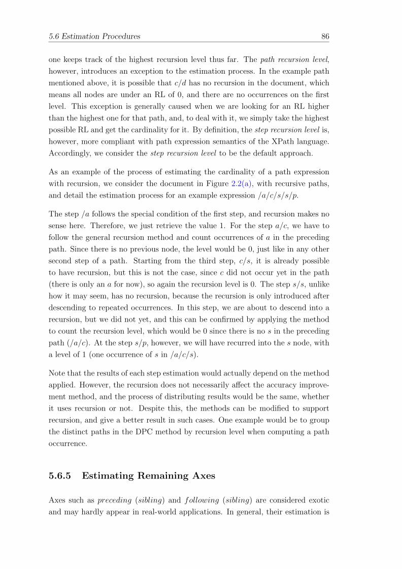
5.6 Estimation Procedures 86

one keeps track of the highest recursion level thus far. The path recursion level,

however, introduces an exception to the estimation process. In the example path

mentioned above, it is possible that c/d has no recursion in the document, which

means all nodes are under an RL of 0, and there are no occurrences on the first

level. This exception is generally caused when we are looking for an RL higher

than the highest one for that path, and, to deal with it, we simply take the highest

possible RL and get the cardinality for it. By definition, the step recursion level is,

however, more compliant with path expression semantics of the XPath language.

Accordingly, we consider the step recursion level to be the default approach.

As an example of the process of estimating the cardinality of a path expression

with recursion, we consider the document in Figure 2.2(a), with recursive paths,

and detail the estimation process for an example expression /a/c/s/s/p.

The step /a follows the special condition of the first step, and recursion makes no

sense here. Therefore, we just retrieve the value 1. For the step a/c, we have to

follow the general recursion method and count occurrences of a in the preceding

path. Since there is no previous node, the level would be 0, just like in any other

second step of a path. Starting from the third step, c/s, it is already possible

to have recursion, but this is not the case, since c did not occur yet in the path

(there is only an a for now), so again the recursion level is 0. The step s/s, unlike

how it may seem, has no recursion, because the recursion is only introduced after

descending to repeated occurrences. In this step, we are about to descend into a

recursion, but we did not yet, and this can be confirmed by applying the method

to count the recursion level, which would be 0 since there is no s in the preceding

path (/a/c). At the step s/p, however, we will have recurred into the s node, with

a level of 1 (one occurrence of s in /a/c/s).

Note that the results of each step estimation would actually depend on the method

applied. However, the recursion does not necessarily affect the accuracy improve-

ment method, and the process of distributing results would be the same, whether

it uses recursion or not. Despite this, the methods can be modified to support

recursion, and give a better result in such cases. One example would be to group

the distinct paths in the DPC method by recursion level when computing a path

occurrence.

5.6.5 Estimating Remaining Axes

Axes such as preceding (sibling) and following (sibling) are considered exotic

and may hardly appear in real-world applications. In general, their estimation is

87 5.6 Estimation Procedures

elusive, because these axes refer to relative positions (order) of node instances.

Hence, the data structures needed would explore this order when collecting statis-

tics for them and would not be maintainable. Indeed, nobody has ever tried to give

estimates for these axes. Nevertheless, we only want to point out here that EXsum

carries some information which could be used and would be helpful, at least for

the upper document levels. Because the root (a) is the first node in document

order, counting all relationships in ASPE(a) delivers the number of the following

elements. When the expression /c/following-sibling::p has to be estimated, we

identify via ASPE(c) the parent of c and, in turn, figure out via the child spoke

of ASPE(a) that there is no sibling p. Of course, we often need to apply some

heuristics at lower levels. For example, expression /t/preceding-sibling::c could be

estimated by accessing the root ASPE(a) and finding in the child spoke that there

is only a single t which has two c nodes as siblings. Because order information is

not available, the number of c nodes in the role of the preceding/following sibling

has to be guessed.

Chapter 6

Experimental Study

Be brave. Take risks. Nothing can substitute experience.

Paulo Coelho, Brazilian novelist, writer, lyricist, and political activist, b.1947

6.1 Introduction

In this chapter, we present our findings regarding the quantitative evaluation of

our proposals. In addition, we comparatively analyze EXsum, LESS, and LWES

against three summaries published in the literature: Markov Tables (MT), XSeed

and Bloom Histogram (BH). All analyses are in regard to the three important

criteria for the query optimization process. This means that in our experiments

we investigate not only the accuracy of a summary, but also the storage needs and

memory footprint, and building and access times.

We define the aim of each criteria throughout this chapter, but first we detail our

set-up environment.

6.2 Setting up

We have implemented and incorporated our approaches and competing ones into

the XDBMS XTC, a native XML database management system. All summaries

have become part of the “Document Metadata” which is maintained by the Meta-

data Component of XTC. This means that for each document evaluated we have

88

89 6.2 Setting up

attached the respective summaries to its metadata1. However, the results pre-

sented here regarding storage do not take into account the overhead of the un-

derlying metadata structure, representing thus the net storage numbers for each

summary.

6.2.1 Documents Considered

XML documents usually exhibit a high degree of redundancy in their structural

part, i.e., they contain many paths having identical sequences of element/attribute

names. To anticipate some characteristics of documents considered in practice, a

well-known set of XML documents is listed in Table 6.1(a).

Table 6.1(b) depicts the structural characteristics of the considered documents.

Column #nodes shows the total number of nodes in a document according to

the DOM specification. Column #E/A shows the number of distinct element/

attribute names. It indicates that only a few of them occur and documents typi-

cally have, therefore, a very repetitive structure. Column max. depth indicates the

highest level that can be reached when traversing the document, while avg. depth

shows the average number of levels in a root-to-leaf path. These last two columns

give some hints on the variability of documents. For example, swissprot is quite

a regular document, because its average depth is close to its maximum depth. In

contrast, treebank is extremely irregular, an exotic outlier. For each document,

columns #homonyms (%PC) and #recursive PC (%PC) contains the detailed

numbers of homonyms path classes and recursive path classes, respectively. The

%PC is the relative quantity of homonyms/recursive path classes in a PS. For

example, the dblp document has 17.07% of homonyms in its PS and only 3.05%

of its path classes are recursive, whereas the xmark document contains 5.48% and

19.7% of homonyms and recursive path classes, respectively. Appendix A studies

in detail homonym distributions in each document considered.

We consider these documents in our comparative experiments of XML summa-

rization structures, as shown later on in Section 6.3.

6.2.2 Test Framework

We created a set of tools to generate, execute, and collect results of XPath query

workloads. We describe these tools in the following.

1The XTC Metadata Component has a underlying B-tree structure.

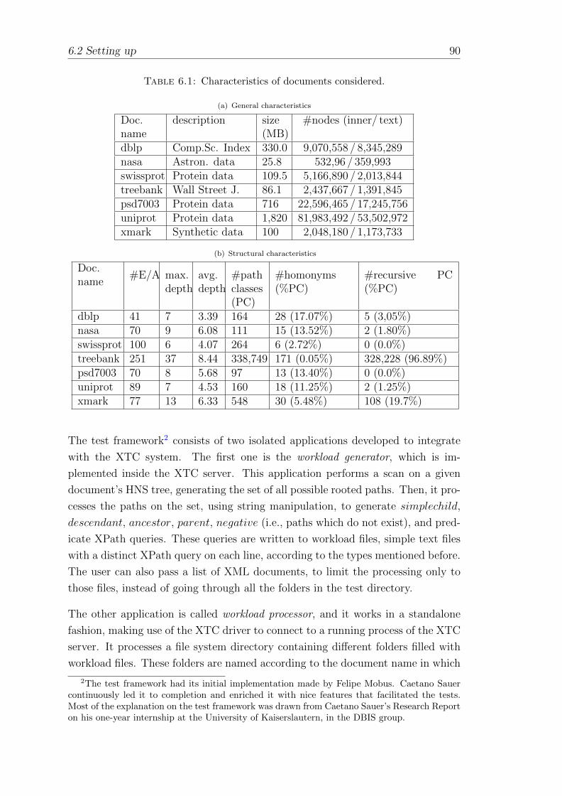
6.2 Setting up 90

Table 6.1: Characteristics of documents considered.

(a) General characteristics

Doc.name

description size(MB)

#nodes (inner/ text)

dblp Comp.Sc. Index 330.0 9,070,558 / 8,345,289nasa Astron. data 25.8 532,96 / 359,993swissprot Protein data 109.5 5,166,890 / 2,013,844treebank Wall Street J. 86.1 2,437,667 / 1,391,845psd7003 Protein data 716 22,596,465 / 17,245,756uniprot Protein data 1,820 81,983,492 / 53,502,972xmark Synthetic data 100 2,048,180 / 1,173,733

(b) Structural characteristics

Doc.name

#E/A max.depth

avg.depth

#pathclasses(PC)

#homonyms(%PC)

#recursive PC(%PC)

dblp 41 7 3.39 164 28 (17.07%) 5 (3,05%)nasa 70 9 6.08 111 15 (13.52%) 2 (1.80%)swissprot 100 6 4.07 264 6 (2.72%) 0 (0.0%)treebank 251 37 8.44 338,749 171 (0.05%) 328,228 (96.89%)psd7003 70 8 5.68 97 13 (13.40%) 0 (0.0%)uniprot 89 7 4.53 160 18 (11.25%) 2 (1.25%)xmark 77 13 6.33 548 30 (5.48%) 108 (19.7%)

The test framework2 consists of two isolated applications developed to integrate

with the XTC system. The first one is the workload generator, which is im-

plemented inside the XTC server. This application performs a scan on a given

document’s HNS tree, generating the set of all possible rooted paths. Then, it pro-

cesses the paths on the set, using string manipulation, to generate simplechild,

descendant, ancestor, parent, negative (i.e., paths which do not exist), and pred-

icate XPath queries. These queries are written to workload files, simple text files

with a distinct XPath query on each line, according to the types mentioned before.

The user can also pass a list of XML documents, to limit the processing only to

those files, instead of going through all the folders in the test directory.

The other application is called workload processor, and it works in a standalone

fashion, making use of the XTC driver to connect to a running process of the XTC

server. It processes a file system directory containing different folders filled with

workload files. These folders are named according to the document name in which

2The test framework had its initial implementation made by Felipe Mobus. Caetano Sauercontinuously led it to completion and enriched it with nice features that facilitated the tests.Most of the explanation on the test framework was drawn from Caetano Sauer’s Research Reporton his one-year internship at the University of Kaiserslautern, in the DBIS group.

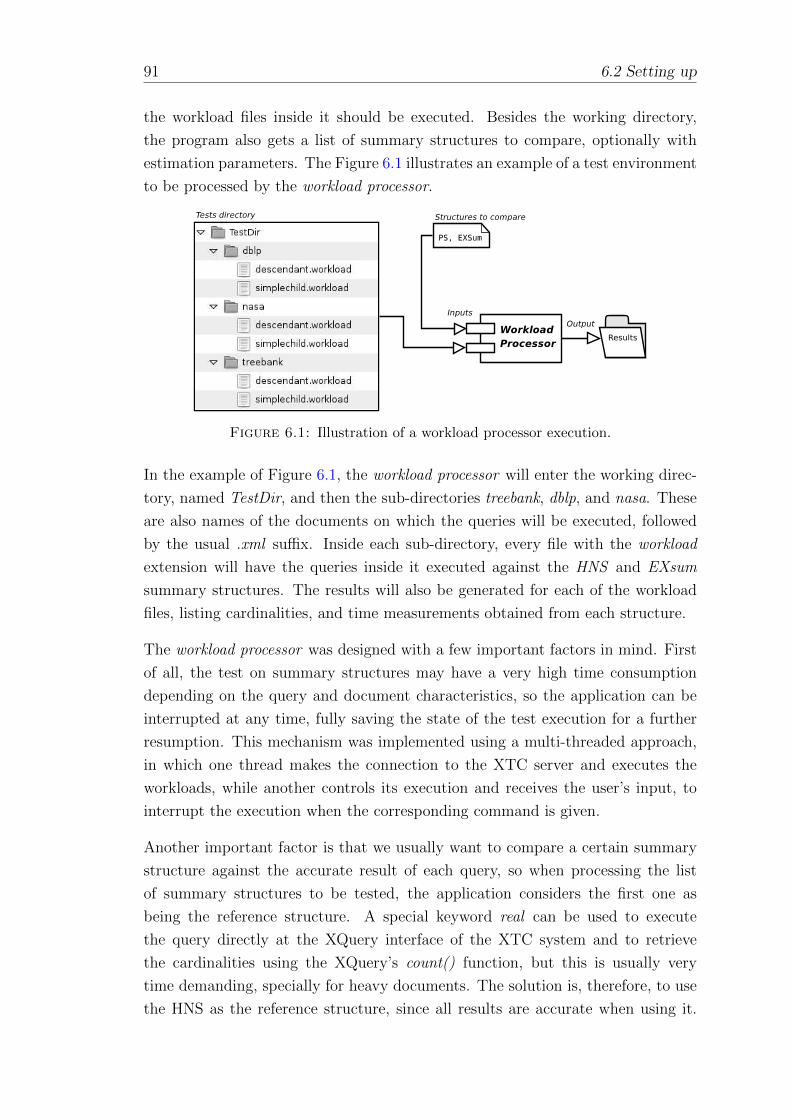
91 6.2 Setting up

the workload files inside it should be executed. Besides the working directory,

the program also gets a list of summary structures to compare, optionally with

estimation parameters. The Figure 6.1 illustrates an example of a test environment

to be processed by the workload processor.

Figure 6.1: Illustration of a workload processor execution.

In the example of Figure 6.1, the workload processor will enter the working direc-

tory, named TestDir, and then the sub-directories treebank, dblp, and nasa. These

are also names of the documents on which the queries will be executed, followed

by the usual .xml suffix. Inside each sub-directory, every file with the workload

extension will have the queries inside it executed against the HNS and EXsum

summary structures. The results will also be generated for each of the workload

files, listing cardinalities, and time measurements obtained from each structure.

The workload processor was designed with a few important factors in mind. First

of all, the test on summary structures may have a very high time consumption

depending on the query and document characteristics, so the application can be

interrupted at any time, fully saving the state of the test execution for a further

resumption. This mechanism was implemented using a multi-threaded approach,

in which one thread makes the connection to the XTC server and executes the

workloads, while another controls its execution and receives the user’s input, to

interrupt the execution when the corresponding command is given.

Another important factor is that we usually want to compare a certain summary

structure against the accurate result of each query, so when processing the list

of summary structures to be tested, the application considers the first one as

being the reference structure. A special keyword real can be used to execute

the query directly at the XQuery interface of the XTC system and to retrieve

the cardinalities using the XQuery’s count() function, but this is usually very

time demanding, specially for heavy documents. The solution is, therefore, to use

the HNS as the reference structure, since all results are accurate when using it.

6.2 Setting up 92

However, for the cases of the parent and ancestor queries and queries with value

predicates, however, one would have to use the actual query execution to obtain

the cardinalities, since HNS lacks support for such queries.

The design of the workload processor application also considers that the documents

may not yet be loaded into the XTC system and the summary structures may not

be stored for them. To cope with this situation, the application makes use of the

connection with the XTC server to test if all the documents provided are stored,

and loading them if they are not. This check considers, however, only the name

of the file, and for the automatic loading to work, the program must receive the

list of documents to process as arguments, and they must include the file system

path. For example, the following call of the workload processor would compare

HNS against EXsum, processing only the documents nasa.xml and treebank.xml:

WorkloadProcessor

/path/to/TestDir

/path/to/nasa.xml,/path/to/treebank.xml

hns,exsum

In this case, the documents nasa.xml and treebank.xml will be checked for existence

in the XTC server, and the path given in the arguments would be used to locate

and load them in case they do not exist. The runXmlStats3 command would also

be executed for HNS and EXSum structures if one of them is not stored in any of

the documents.

6.2.3 Query Workload

Using the workload generator and for each document listed in Table 6.1(a), we have

produced a query workload with respect to the following types of queries: sim-

plechild, descendant, parent, and ancestor queries. Simplechild queries encompass

only child (/) axes. The amount of simplechild queries produced for each docu-

ment, except for treebank, covers all possible paths in the document. Descendant,

parent and ancestor queries have been randomized.

3We have created four commands in the XTC system to collect and generate sum-maries (runXmlStats), view a summary created (viewXmlStats), delete an existing sum-mary (deleteXmlStats), and list the stored summaries (listXmlStats). These commandscompound the estimation interface of the XTC. Additionally, there are two other commands,estimateExpression and estimateStep which are designed to be integrated to the query opti-mizer.

93 6.2 Setting up

For treebank, due to its huge number of path classes, we randomized the entire

workload. Additionally, we have generated queries containing structural and value

predicates. For queries with value predicates, we directed the generation of work-

load to a biased way. That is, we have generated value predicates with a ratio

of 60:40. This means that we generated 60% of the predicates among the most

frequent entries in the frequency vector and randomized the 40% remaining among

the least frequent entries.

6.2.4 Configuring Parameters

For comparing EXsum, LWES, and LESS against the competing approaches:

XSeed, Markov Table (MT), and Bloom Histogram (BH), we have chosen the

following settings.

For Markov Tables, we have evaluated two values of the pruning parameter: 2

(MT2) and 3 (MT3). We have used the MT compression method called suffix-

star. Additionally, we have set the memory budget (in number of MT entries) for

MT2 and MT3, of 90 and 30, respectively.

For the XSeed kernel, we have set the search pruning parameter to 100 for treebank,

50 for dblp, and 20 for the other documents.

For LWES, End-biased histograms were continuously applied to all levels of the

summary structure.

BH has been tested with Bloom filters of 125 bytes (1,000 bits) for all buckets

using 10 hash functions, resulting in a false positive rate of approximately 10−6 in

the majority of the cases. The number of buckets for BH has been set to 1/4 of

the entries of the path-count table for all documents except treebank, which was

set to ten4.

6.2.5 Hardware and Software Environment for Testing

Before introducing the test results generated by the workload processor, we will

first describe the test environment, including hardware, software, and operating

system characteristics.

4The reason to limit the number of BH buckets for treebank is that its building algorithm hasa quadratic complexity in the number of path classes — and treebank has more than 600,000path classes. We have tested using 1/4 of the path-count table but BH building could not finish,even with a fewer number of buckets. Therefore, as we could only build BH with 10 buckets fortreebank, we have used this configuration.

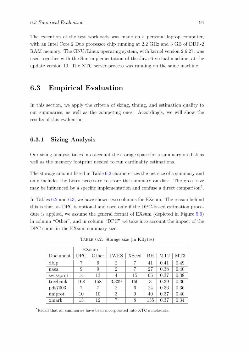
6.3 Empirical Evaluation 94

The execution of the test workloads was made on a personal laptop computer,

with an Intel Core 2 Duo processor chip running at 2.2 GHz and 3 GB of DDR-2

RAM memory. The GNU/Linux operating system, with kernel version 2.6.27, was

used together with the Sun implementation of the Java 6 virtual machine, at the

update version 10. The XTC server process was running on the same machine.

6.3 Empirical Evaluation

In this section, we apply the criteria of sizing, timing, and estimation quality to

our summaries, as well as the competing ones. Accordingly, we will show the

results of this evaluation.

6.3.1 Sizing Analysis

Our sizing analysis takes into account the storage space for a summary on disk as

well as the memory footprint needed to run cardinality estimations.

The storage amount listed in Table 6.2 characterizes the net size of a summary and

only includes the bytes necessary to store the summary on disk. The gross size

may be influenced by a specific implementation and confuse a direct comparison5.

In Tables 6.2 and 6.3, we have shown two columns for EXsum. The reason behind

this is that, as DPC is optional and used only if the DPC-based estimation proce-

dure is applied, we assume the general format of EXsum (depicted in Figure 5.6)

in column “Other”, and in column “DPC” we take into account the impact of the

DPC count in the EXsum summary size.

Table 6.2: Storage size (in KBytes)

EXsumDocument DPC Other LWES XSeed BH MT2 MT3

dblp 7 6 2 7 41 0.41 0.49nasa 9 9 2 7 27 0.38 0.40swissprot 14 13 4 15 65 0.37 0.38treebank 168 158 3,339 160 3 0.39 0.36pds7003 7 7 2 6 24 0.36 0.36uniprot 10 10 3 9 40 0.37 0.40xmark 13 12 7 8 135 0.37 0.34

5Recall that all summaries have been incorporated into XTC’s metadata.

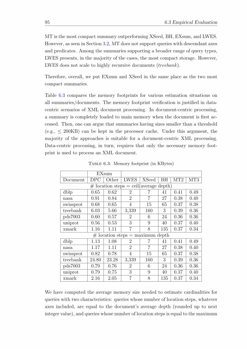
95 6.3 Empirical Evaluation

MT is the most compact summary outperforming XSeed, BH, EXsum, and LWES.

However, as seen in Section 3.2, MT does not support queries with descendant axes

and predicates. Among the summaries supporting a broader range of query types,

LWES presents, in the majority of the cases, the most compact storage. However,

LWES does not scale to highly recursive documents (treebank).

Therefore, overall, we put EXsum and XSeed in the same place as the two most

compact summaries.

Table 6.3 compares the memory footprints for various estimation situations on

all summaries/documents. The memory footprint verification is justified in data-

centric scenarios of XML document processing. In document-centric processing,

a summary is completely loaded to main memory when the document is first ac-

cessed. Then, one can argue that summaries having sizes smaller than a threshold

(e.g., ≤ 200KB) can be kept in the processor cache. Under this argument, the

majority of the approaches is suitable for a document-centric XML processing.

Data-centric processing, in turn, requires that only the necessary memory foot-

print is used to process an XML document.

Table 6.3: Memory footprint (in KBytes)

EXsumDocument DPC Other LWES XSeed BH MT2 MT3

# location steps = ceil(average depth)dblp 0.65 0.62 2 7 41 0.41 0.49nasa 0.91 0.84 2 7 27 0.38 0.40swissprot 0.68 0.65 4 15 65 0.37 0.38treebank 6.03 5.66 3,339 160 3 0.39 0.36pds7003 0.60 0.57 2 6 24 0.36 0.36uniprot 0.56 0.53 3 9 40 0.37 0.40xmark 1.16 1.11 7 8 135 0.37 0.34

# location steps = maximum depthdblp 1.13 1.08 2 7 41 0.41 0.49nasa 1.17 1.11 2 7 27 0.38 0.40swissprot 0.82 0.78 4 15 65 0.37 0.38treebank 24.80 23.28 3,339 160 3 0.39 0.36pds7003 0.79 0.76 2 6 24 0.36 0.36uniprot 0.79 0.75 3 9 40 0.37 0.40xmark 2.16 2.05 7 8 135 0.37 0.34

We have computed the average memory size needed to estimate cardinalities for

queries with two characteristics: queries whose number of location steps, whatever

axes included, are equal to the document’s average depth (rounded up to next

integer value), and queries whose number of location steps is equal to the maximum

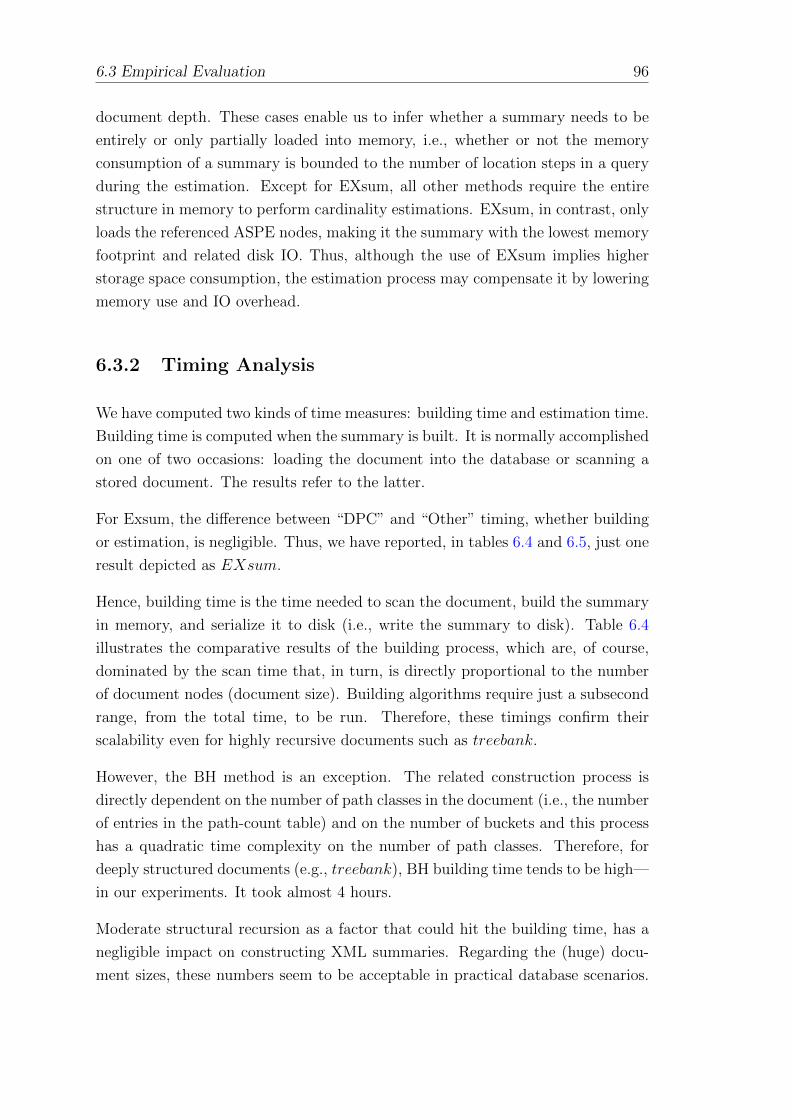
6.3 Empirical Evaluation 96

document depth. These cases enable us to infer whether a summary needs to be

entirely or only partially loaded into memory, i.e., whether or not the memory

consumption of a summary is bounded to the number of location steps in a query

during the estimation. Except for EXsum, all other methods require the entire

structure in memory to perform cardinality estimations. EXsum, in contrast, only

loads the referenced ASPE nodes, making it the summary with the lowest memory

footprint and related disk IO. Thus, although the use of EXsum implies higher

storage space consumption, the estimation process may compensate it by lowering

memory use and IO overhead.

6.3.2 Timing Analysis

We have computed two kinds of time measures: building time and estimation time.

Building time is computed when the summary is built. It is normally accomplished

on one of two occasions: loading the document into the database or scanning a

stored document. The results refer to the latter.

For Exsum, the difference between “DPC” and “Other” timing, whether building

or estimation, is negligible. Thus, we have reported, in tables 6.4 and 6.5, just one

result depicted as EXsum.

Hence, building time is the time needed to scan the document, build the summary

in memory, and serialize it to disk (i.e., write the summary to disk). Table 6.4

illustrates the comparative results of the building process, which are, of course,

dominated by the scan time that, in turn, is directly proportional to the number

of document nodes (document size). Building algorithms require just a subsecond

range, from the total time, to be run. Therefore, these timings confirm their

scalability even for highly recursive documents such as treebank.

However, the BH method is an exception. The related construction process is

directly dependent on the number of path classes in the document (i.e., the number

of entries in the path-count table) and on the number of buckets and this process

has a quadratic time complexity on the number of path classes. Therefore, for

deeply structured documents (e.g., treebank), BH building time tends to be high—

in our experiments. It took almost 4 hours.

Moderate structural recursion as a factor that could hit the building time, has a

negligible impact on constructing XML summaries. Regarding the (huge) docu-

ment sizes, these numbers seem to be acceptable in practical database scenarios.

97 6.3 Empirical Evaluation

For example, the worst time verified (EXsum for a non-recursive 1GB-uniprot doc-

ument) corresponds to 18.3 minutes, whereas the worst case for treebank (LWES)

corresponds to 2.3 minutes.

Table 6.4: Building times (in sec)

Document EXsum LWES XSeed BH MT2 MT3

dblp 121.81 86.31 135.51 217.10 85.99 85.97nasa 10.35 5.47 5.43 11.48 5.19 5.20swissprot 63.67 37.65 53.73 102.77 37.45 37.71treebank 59.83 138.79 42.88 13,458.0 45.96 45.82pds7003 941.95 653.53 715.71 1,393.82 653.56 653.52uniprot 1,096.75 486.74 779.35 1,089.96 486.60 486.62xmark 51.07 25.07 55.61 62.05 25.06 25.06

Estimation time refers to the time needed to estimate a query. That is, the time

that the estimation process needs to get the query expression, access the summary

(possibly, more than once), and report the result to the optimizer. The time

considered here is an arithmetic average of the times required by every query in

the workload. Table 6.5 presents the estimation times classified by query types.

EXsum delivers the superior results for all document and query types; hence, its

impact on the overall optimization process is very low. XSeed and LWES have

prohibitive times for queries with descendant axes in deeply structure documents,

whereas, for the other documents, their times are acceptable.

The problem with LWES and XSeed is the traversal of their structures when

they have to be used to estimate descendant axes for highly recursive or deeply-

structured documents. Although the XSeed estimation procedures make a trade-

off between estimation time and accuracy by setting a tuning parameter—thereby

producing fast results at expenses of low estimation quality—LWES seems to have

a costly search in its parent pointers to qualify nodes in estimating descendant

axes.

6.3.3 Estimation Quality

Estimation quality refers to the accuracy of a summary, or the ability to provide

cardinality estimations near the actual values and is expressed by an error metric.

In our case, we used the Normalized Root Mean Square Error (NRMSE) which is

defined by the formula:√∑n

i=1(ei − ai)2/(∑n

i=1(ai)/n), where n is the number of

queries in the workload, e is the estimated result size and a is the actual result

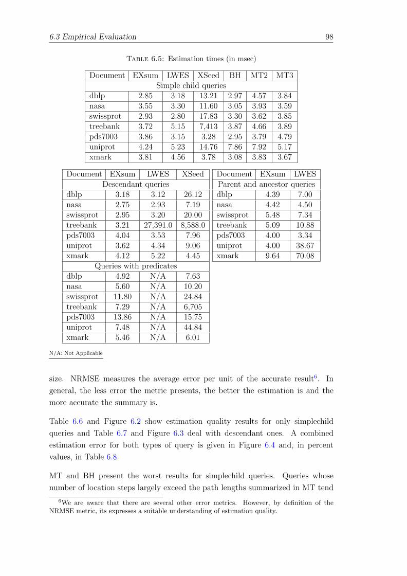
6.3 Empirical Evaluation 98

Table 6.5: Estimation times (in msec)

Document EXsum LWES XSeed BH MT2 MT3Simple child queries

dblp 2.85 3.18 13.21 2.97 4.57 3.84nasa 3.55 3.30 11.60 3.05 3.93 3.59swissprot 2.93 2.80 17.83 3.30 3.62 3.85treebank 3.72 5.15 7,413 3.87 4.66 3.89pds7003 3.86 3.15 3.28 2.95 3.79 4.79uniprot 4.24 5.23 14.76 7.86 7.92 5.17xmark 3.81 4.56 3.78 3.08 3.83 3.67

Document EXsum LWES XSeedDescendant queries

dblp 3.18 3.12 26.12nasa 2.75 2.93 7.19swissprot 2.95 3.20 20.00treebank 3.21 27,391.0 8,588.0pds7003 4.04 3.53 7.96uniprot 3.62 4.34 9.06xmark 4.12 5.22 4.45

Queries with predicatesdblp 4.92 N/A 7.63nasa 5.60 N/A 10.20swissprot 11.80 N/A 24.84treebank 7.29 N/A 6,705pds7003 13.86 N/A 15.75uniprot 7.48 N/A 44.84xmark 5.46 N/A 6.01

Document EXsum LWESParent and ancestor queriesdblp 4.39 7.00nasa 4.42 4.50swissprot 5.48 7.34treebank 5.09 10.88pds7003 4.00 3.34uniprot 4.00 38.67xmark 9.64 70.08

N/A: Not Applicable

size. NRMSE measures the average error per unit of the accurate result6. In

general, the less error the metric presents, the better the estimation is and the

more accurate the summary is.

Table 6.6 and Figure 6.2 show estimation quality results for only simplechild

queries and Table 6.7 and Figure 6.3 deal with descendant ones. A combined

estimation error for both types of query is given in Figure 6.4 and, in percent

values, in Table 6.8.

MT and BH present the worst results for simplechild queries. Queries whose

number of location steps largely exceed the path lengths summarized in MT tend

6We are aware that there are several other error metrics. However, by definition of theNRMSE metric, its expresses a suitable understanding of estimation quality.

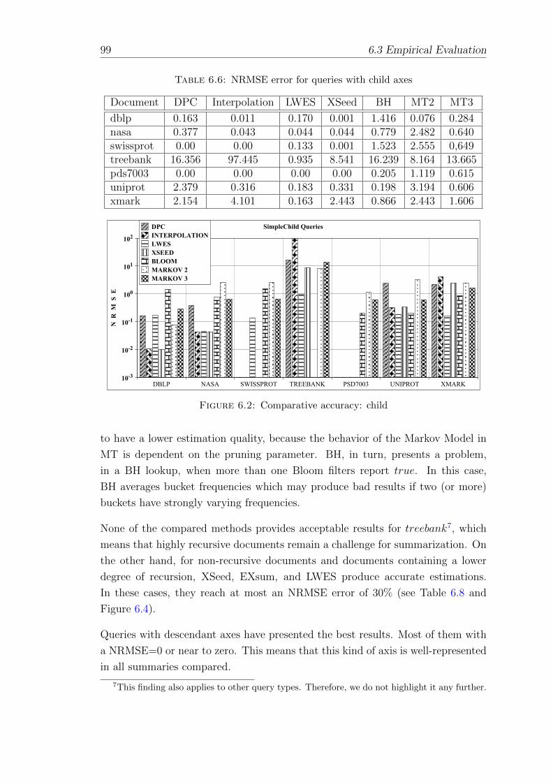
99 6.3 Empirical Evaluation

Table 6.6: NRMSE error for queries with child axes

Document DPC Interpolation LWES XSeed BH MT2 MT3

dblp 0.163 0.011 0.170 0.001 1.416 0.076 0.284nasa 0.377 0.043 0.044 0.044 0.779 2.482 0.640swissprot 0.00 0.00 0.133 0.001 1.523 2.555 0,649treebank 16.356 97.445 0.935 8.541 16.239 8.164 13.665pds7003 0.00 0.00 0.00 0.00 0.205 1.119 0.615uniprot 2.379 0.316 0.183 0.331 0.198 3.194 0.606xmark 2.154 4.101 0.163 2.443 0.866 2.443 1.606

DBLP NASA SWISSPROT TREEBANK PSD7003 UNIPROT XMARK

10-3

10-2

10-1

100

101

102

N

R

M S

E

SimpleChild QueriesDPC

INTERPOLATION

LWES

XSEED

BLOOM

MARKOV 2

MARKOV 3

Figure 6.2: Comparative accuracy: child

to have a lower estimation quality, because the behavior of the Markov Model in

MT is dependent on the pruning parameter. BH, in turn, presents a problem,

in a BH lookup, when more than one Bloom filters report true. In this case,

BH averages bucket frequencies which may produce bad results if two (or more)

buckets have strongly varying frequencies.

None of the compared methods provides acceptable results for treebank7, which

means that highly recursive documents remain a challenge for summarization. On

the other hand, for non-recursive documents and documents containing a lower

degree of recursion, XSeed, EXsum, and LWES produce accurate estimations.

In these cases, they reach at most an NRMSE error of 30% (see Table 6.8 and

Figure 6.4).

Queries with descendant axes have presented the best results. Most of them with

a NRMSE=0 or near to zero. This means that this kind of axis is well-represented

in all summaries compared.

7This finding also applies to other query types. Therefore, we do not highlight it any further.

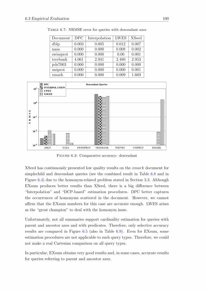
6.3 Empirical Evaluation 100

Table 6.7: NRMSE error for queries with descendant axes

Document DPC Interpolation LWES XSeed

dblp 0.003 0.005 0.012 0.007nasa 0.000 0.000 0.008 0.002swissprot 0.000 0.000 0.00 0.001treebank 4.061 2.941 2.480 2.953pds7003 0.000 0.000 0.000 0.000uniprot 0.000 0.000 0.000 0.001xmark 0.000 0.000 0.009 1.669

DBLP NASA SWISSPROT TREEBANK PSD7003 UNIPROT XMARK

10-3

10-2

10-1

100

101

N R

M

S

E

Descendant QueriesDPC

INTERPOLATION

LWES

XSEED

Figure 6.3: Comparative accuracy: descendant

XSeed has continuously presented low quality results on the xmark document for

simplechild and descendant queries (see the combined result in Table 6.8 and in

Figure 6.4) due to the homonym-related problem stated in Section 3.3. Although

EXsum produces better results than XSeed, there is a big difference between

“Interpolation” and “DCP-based” estimation procedures. DPC better captures

the occurrences of homonyms scattered in the document. However, we cannot

affirm that the EXsum numbers for this case are accurate enough. LWES arises

as the “great champion” to deal with the homonym issue.

Unfortunately, not all summaries support cardinality estimation for queries with

parent and ancestor axes and with predicates. Therefore, only selective accuracy

results are compared in Figure 6.5 (also in Table 6.9). Even for EXsum, some

estimation procedures are not applicable to such query types. Therefore, we could

not make a real Cartesian comparison on all query types.

In particular, EXsum obtains very good results and, in some cases, accurate results

for queries referring to parent and ancestor axes.

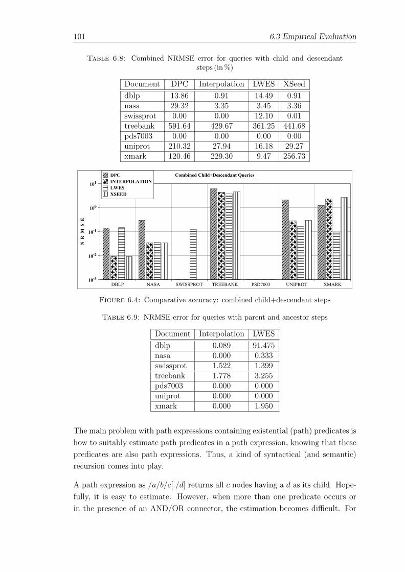
101 6.3 Empirical Evaluation

Table 6.8: Combined NRMSE error for queries with child and descendantsteps (in %)

Document DPC Interpolation LWES XSeed

dblp 13.86 0.91 14.49 0.91nasa 29.32 3.35 3.45 3.36swissprot 0.00 0.00 12.10 0.01treebank 591.64 429.67 361.25 441.68pds7003 0.00 0.00 0.00 0.00uniprot 210.32 27.94 16.18 29.27xmark 120.46 229.30 9.47 256.73

DBLP NASA SWISSPROT TREEBANK PSD7003 UNIPROT XMARK

10-3

10-2

10-1

100

101

N

R

M

S E

Combined Child+Descendant QueriesDPC

INTERPOLATION

LWES

XSEED

Figure 6.4: Comparative accuracy: combined child+descendant steps

Table 6.9: NRMSE error for queries with parent and ancestor steps

Document Interpolation LWES

dblp 0.089 91.475nasa 0.000 0.333swissprot 1.522 1.399treebank 1.778 3.255pds7003 0.000 0.000uniprot 0.000 0.000xmark 0.000 1.950

The main problem with path expressions containing existential (path) predicates is

how to suitably estimate path predicates in a path expression, knowing that these

predicates are also path expressions. Thus, a kind of syntactical (and semantic)

recursion comes into play.

A path expression as /a/b/c[./d] returns all c nodes having a d as its child. Hope-

fully, it is easy to estimate. However, when more than one predicate occurs or

in the presence of an AND/OR connector, the estimation becomes difficult. For

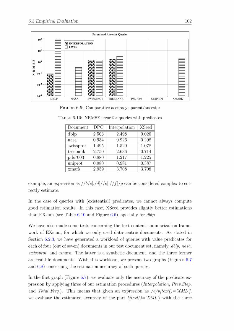
6.3 Empirical Evaluation 102

DBLP NASA SWISSPROT TREEBANK PSD7003 UNIPROT XMARK

10-3

10-2

10-1

100

101

102

N R

M

S

E

Parent and Ancestor Queries

INTERPOLATION

LWES

Figure 6.5: Comparative accuracy: parent/ancestor

Table 6.10: NRMSE error for queries with predicates

Document DPC Interpolation XSeed

dblp 2.503 2.498 0.020nasa 0.934 0.926 0.298swissprot 1.495 1.520 1.078treebank 2.750 2.636 0.714pds7003 0.880 1.217 1.225uniprot 0.980 0.981 0.387xmark 2.959 3.708 3.708

example, an expression as //b/c[./d]//e[.//f ]/g can be considered complex to cor-

rectly estimate.

In the case of queries with (existential) predicates, we cannot always compute

good estimation results. In this case, XSeed provides slightly better estimations

than EXsum (see Table 6.10 and Figure 6.6), specially for dblp.

We have also made some tests concerning the text content summarization frame-

work of EXsum, for which we only used data-centric documents. As stated in

Section 6.2.3, we have generated a workload of queries with value predicates for

each of four (out of seven) documents in our test document set, namely, dblp, nasa,

swissprot, and xmark. The latter is a synthetic document, and the three former

are real-life documents. With this workload, we present two graphs (Figures 6.7

and 6.8) concerning the estimation accuracy of such queries.

In the first graph (Figure 6.7), we evaluate only the accuracy of the predicate ex-

pression by applying three of our estimation procedures (Interpolation, Prev.Step,

and Total Freq.). This means that given an expression as /a/b[text()=’XML’],

we evaluate the estimated accuracy of the part b[text()=’XML’] with the three

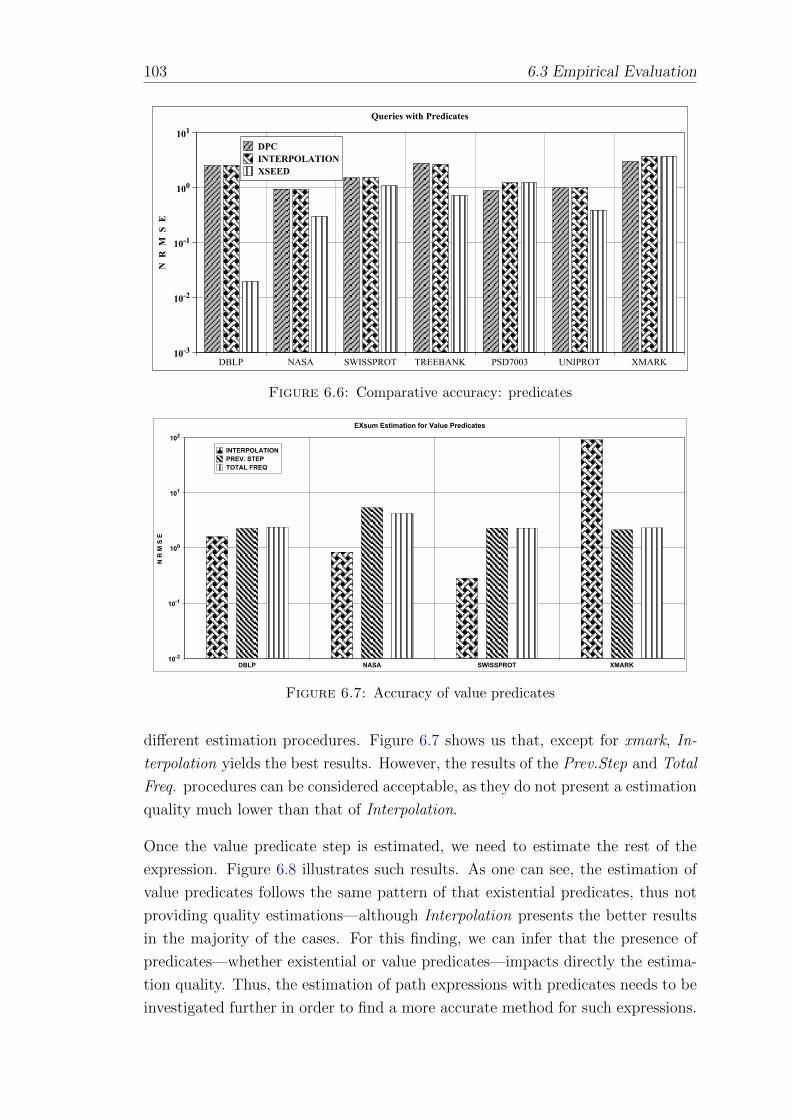
103 6.3 Empirical Evaluation

DBLP NASA SWISSPROT TREEBANK PSD7003 UNIPROT XMARK

10-3

10-2

10-1

100

101

N R

M

S

E

Queries with Predicates

DPC

INTERPOLATION

XSEED

Figure 6.6: Comparative accuracy: predicates

DBLP NASA SWISSPROT XMARK10-2

10-1

100

101

102

N R

M S

E

EXsum Estimation for Value Predicates

INTERPOLATION

PREV. STEP

TOTAL FREQ

Figure 6.7: Accuracy of value predicates

different estimation procedures. Figure 6.7 shows us that, except for xmark, In-

terpolation yields the best results. However, the results of the Prev.Step and Total

Freq. procedures can be considered acceptable, as they do not present a estimation

quality much lower than that of Interpolation.

Once the value predicate step is estimated, we need to estimate the rest of the

expression. Figure 6.8 illustrates such results. As one can see, the estimation of

value predicates follows the same pattern of that existential predicates, thus not

providing quality estimations—although Interpolation presents the better results

in the majority of the cases. For this finding, we can infer that the presence of

predicates—whether existential or value predicates—impacts directly the estima-

tion quality. Thus, the estimation of path expressions with predicates needs to be

investigated further in order to find a more accurate method for such expressions.

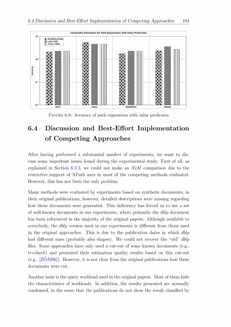
6.4 Discussion and Best-Effort Implementation of Competing Approaches 104

DBLP NASA SWISSPROT XMARK10-2

10-1

100

101

N R

M S

ECardinality Estimation for Path Expressions with Value Predicates

INTERPOLATION

LAST STEP

TOTAL FREQ

Figure 6.8: Accuracy of path expressions with value predicates

6.4 Discussion and Best-Effort Implementation

of Competing Approaches

After having performed a substantial number of experiments, we want to dis-

cuss some important issues found during the experimental study. First of all, as

explained in Section 6.3.3, we could not make an NxM comparison due to the

restrictive support of XPath axes in most of the competing methods evaluated.

However, this has not been the only problem.

Many methods were evaluated by experiments based on synthetic documents; in

their original publications, however, detailed descriptions were missing regarding

how these documents were generated. This deficiency has forced us to use a set

of well-known documents in our experiments, where primarily the dblp document

has been referenced in the majority of the original papers. Although available to

everybody, the dblp version used in our experiments is different from those used

in the original approaches. This is due to the publication dates in which dblp

had different sizes (probably also shapes). We could not recover the “old” dblp

files. Some approaches have only used a cut-out of some known documents (e.g.,

treebank) and presented their estimation quality results based on this cut-out

(e.g., [ZOAI06]). However, it is not clear from the original publications how these

documents were cut.

Another issue is the query workload used in the original papers. Most of them hide

the characteristics of workloads. In addition, the results presented are normally

condensed, in the sense that the publications do not show the result classified by

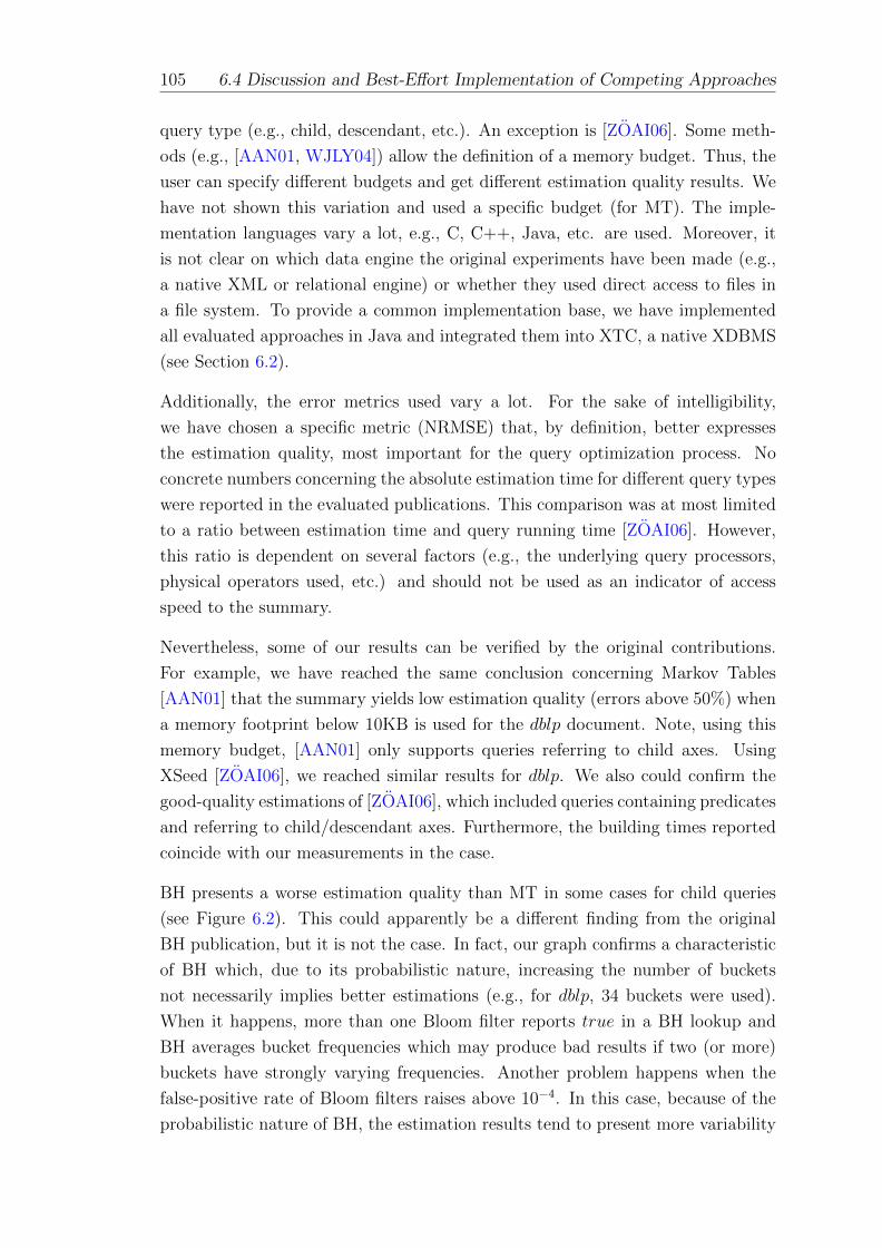
105 6.4 Discussion and Best-Effort Implementation of Competing Approaches

query type (e.g., child, descendant, etc.). An exception is [ZOAI06]. Some meth-

ods (e.g., [AAN01, WJLY04]) allow the definition of a memory budget. Thus, the

user can specify different budgets and get different estimation quality results. We

have not shown this variation and used a specific budget (for MT). The imple-

mentation languages vary a lot, e.g., C, C++, Java, etc. are used. Moreover, it

is not clear on which data engine the original experiments have been made (e.g.,

a native XML or relational engine) or whether they used direct access to files in

a file system. To provide a common implementation base, we have implemented

all evaluated approaches in Java and integrated them into XTC, a native XDBMS

(see Section 6.2).

Additionally, the error metrics used vary a lot. For the sake of intelligibility,

we have chosen a specific metric (NRMSE) that, by definition, better expresses

the estimation quality, most important for the query optimization process. No

concrete numbers concerning the absolute estimation time for different query types

were reported in the evaluated publications. This comparison was at most limited

to a ratio between estimation time and query running time [ZOAI06]. However,

this ratio is dependent on several factors (e.g., the underlying query processors,

physical operators used, etc.) and should not be used as an indicator of access

speed to the summary.

Nevertheless, some of our results can be verified by the original contributions.

For example, we have reached the same conclusion concerning Markov Tables

[AAN01] that the summary yields low estimation quality (errors above 50%) when

a memory footprint below 10KB is used for the dblp document. Note, using this

memory budget, [AAN01] only supports queries referring to child axes. Using

XSeed [ZOAI06], we reached similar results for dblp. We also could confirm the

good-quality estimations of [ZOAI06], which included queries containing predicates

and referring to child/descendant axes. Furthermore, the building times reported

coincide with our measurements in the case.

BH presents a worse estimation quality than MT in some cases for child queries

(see Figure 6.2). This could apparently be a different finding from the original

BH publication, but it is not the case. In fact, our graph confirms a characteristic

of BH which, due to its probabilistic nature, increasing the number of buckets

not necessarily implies better estimations (e.g., for dblp, 34 buckets were used).

When it happens, more than one Bloom filter reports true in a BH lookup and

BH averages bucket frequencies which may produce bad results if two (or more)

buckets have strongly varying frequencies. Another problem happens when the

false-positive rate of Bloom filters raises above 10−4. In this case, because of the

probabilistic nature of BH, the estimation results tend to present more variability

6.4 Discussion and Best-Effort Implementation of Competing Approaches 106

than that with low false-positive error rate. The balance between the number of

buckets and the false-positive rate for looking up BH is, in our humble opinion,

difficult to reach in practical scenarios.

Chapter 7

Conclusions and Outlook

No amount of experimentation can ever prove me right; a single experiment can prove me

wrong.

Albert Einstein, German Physicist, 1879 – 1955

After having studied the XML summarization problems, having proposed three

solutions, namely, LESS, LWES, and EXsum, and empirically compared them

with some competitor approaches, we want to conclude our work.

XML summarization remains yet an open problem in its general concept. Com-

pressing value and structure of an XML document to provide good estimates in

the majority of the cases (or, at least, in the common cases) is neither a simple,

nor an easy task. The most difficult issue to be tackled is the document order and,

consequently, the possible axes derived, but it is not the only issue.

7.1 Main Results

The variability expected whether in structure or in values in an XML document

is high. We should consider skewness as a rule, not as an exception. Taking only

the structure into account, we have presented two factors which make it difficult

to reach quality estimations: structural recursion and homonyms. However, we

are aware that these factors may not be the only ones.

We have used, in LESS and LWES summaries, the well-known compression tech-

nique called histogram and studied the many types of histograms to be applied.

107

7.2 Future Research 108

However, accuracy loses its power for a query optimization process if other impor-

tant characteristics are not verified as well. With our initial insight on LESS and

LWES, we wanted to find a new way to summarize XML documents.

This way is substantiated in the EXsum summary which brings, besides accuracy,

positive and important features regarding its use for a query optimizer as scal-

ability in its size. For example, the summary size do not have a strict relation

to the document size, fast access, or low memory footprint. The EXsum sum-

mary provides a simple (and hopefully, intuitive) manner to approximate an XML

document. Additionally, it is extensible enough to encompass value-and-structure

summarizations.

We cannot obviously state that, considering all parameters involved in providing

XML summaries for their use in the query optimization area, our proposals are the

very champion among others published in the literature. However, we expect that

at least EXsum, due to its nature, may have a place in a multi-user, full-fledged

native XML database in the future.

7.2 Future Research

While the cost-based query optimizer of XTC is under development, we expect

that our proposals can be integrated into it, thus, forming a complete XML cost-

based query evaluation component. In fact, our design and implementation have

been driven to this aim. It should be verified for the estimation of text predicates—

using Information Retrieval assumptions—under varying scenarios of data-centric

documents. Furthermore, to identify new problems, it could be extended towards

longer text values ending up in document-centric characteristics.

In addition, we can realize at least three different areas to apply the concepts

presented here. For example, one of the well-known flaws of a RDBMS query

engine is how to correctly estimate a join operation. Nowadays, an independence

assumption is made and a join predicate, between tables R and S, as R.a =

S.a is estimated assuming there is no correlation between R.a and S.a. This

is, in practice, not justified in all the cases, mostly when a join encompasses

tables linked by a referential integrity constraint. In such case, there is really

a correlation between the tables, and the actual estimation method may lead to

an underestimation of the join result. The same applies to self-joins. Another

problem comes with recursion provided by the With Recursive SQL clause. Only

109 7.2 Future Research

linear recursion is permitted in SQL and, even though, the recursive clause is

rewritten into a set of joins—sometimes correlated joins.

In such cases, LWES and EXsum structures can improve the estimation quality

because they capture the correlation among values. EXsum, due to its captur-

ing of binary relationships among values (see EXsum’s construction principle in

Section 5.3), is particularly suitable to be adapted for its use in an RDBMS join

estimation process. Therefore, the use of EXsum in these cases might eliminate

the independence assumption, and, hopefully, may yield better results.

In the Data Warehouse area, specifically in ROLAP (Relational On-Line Analyt-

ical Processing), the cube estimation, i.e., the estimated storage requirements for

the cube size, is yet an area in which we can give some contributions. Most fre-

quently, cubes in DW/ROLAP databases are a result of the so-called star-queries,

i.e., queries with a pattern involving necessarily the fact table and two or more

dimension tables. The resulting aggregation is a direct application of the CUBE

and ROLLUP SQL clauses—in fact, subclauses of the Group By. Thus, the num-

ber of attributes in dimensions that intersect the measure group may be estimated

and, consequently, the cube size, if we use EXsum by modeling each ASPE node

as an attribute value and the spokes as the possible intersections.

Of course, we are aware that some heuristic-based star-query techniques may be,

in addition, applied and also some compression techniques that may influence the

estimation results.

Last but not least, cost-based query processing in sensor data management may

benefit from our proposals. A sensor normally collects data as temperature, air

pressure, humidity, etc. A sensor network has a (common) hierarchical topol-

ogy, called routing tree overlay in sensor data management terminology, with a

parent-child relationship among sensors (nodes). If a query is posed (and partially

processed) in a base station—most probably a PC-based computer—we can esti-

mate such a query by using, for example, LWES to model sensors in the routing

tree overlay where each LWES node, corresponding to a sensor (or a set of sensors),

might have the summarized data collected by the sensor.

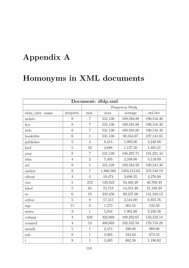
Appendix A

Homonyms in XML documents

Document: dblp.xmlFrequency Study

elem./attr. name #repetit. min. max. average std.dev

mdate 8 7 531,130 109,594.88 190,516.40

key 8 7 531,130 109,594.88 190,516.40

title 8 7 531,130 109,594.88 190,516.40

booktitle 6 1 531,130 90,354.67 197,141.85

publisher 5 4 8,415 1,993.00 3,240.98

href 5 59 4,888 1,137.20 1,885.21

year 8 7 531,130 108,297.75 191,221.44

isbn 4 2 7,495 2,168.00 3,110.09

url 8 1 531,128 109,344.50 190,541.38

author 8 7 1,366,560 1263,213.63 478,548.19

cdrom 4 4 10,474 3,698.25 4,276.80

cite 5 212 120,822 34,480.20 46,700.49

label 5 65 55,718 14,551.40 21,188.29

ee 6 10 332,456 89,237.00 131,583.13

editor 5 8 17,415 3,544.80 6,935.76

sup 11 2 1,575 264.55 532.50

series 3 1 5,044 1,901.00 2,238.56

volume 3 620 322,060 109,202.67 150,523.14

crossref 4 13 408,603 102,522.50 176,716.28

month 5 1 2,474 496.00 989.00

sub 8 1 2,065 344.63 672.52

i 8 1 3,485 682.38 1,190.62

110

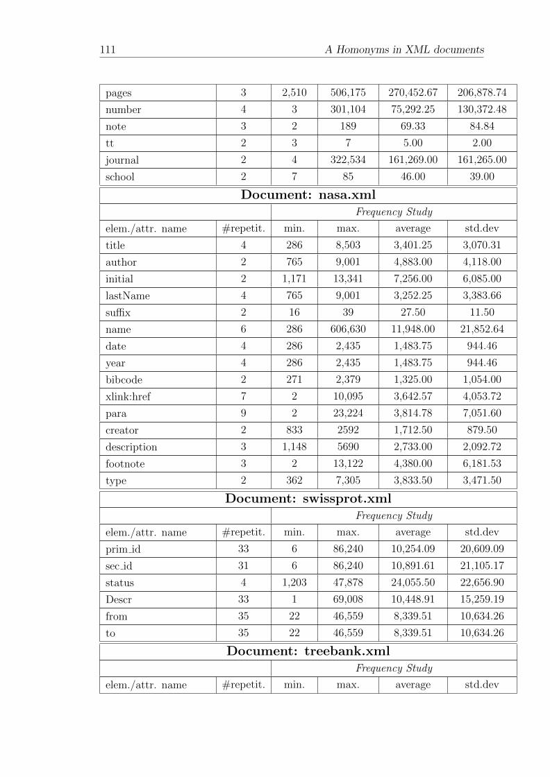
111 A Homonyms in XML documents

pages 3 2,510 506,175 270,452.67 206,878.74

number 4 3 301,104 75,292.25 130,372.48

note 3 2 189 69.33 84.84

tt 2 3 7 5.00 2.00

journal 2 4 322,534 161,269.00 161,265.00

school 2 7 85 46.00 39.00

Document: nasa.xmlFrequency Study

elem./attr. name #repetit. min. max. average std.dev

title 4 286 8,503 3,401.25 3,070.31

author 2 765 9,001 4,883.00 4,118.00

initial 2 1,171 13,341 7,256.00 6,085.00

lastName 4 765 9,001 3,252.25 3,383.66

suffix 2 16 39 27.50 11.50

name 6 286 606,630 11,948.00 21,852.64

date 4 286 2,435 1,483.75 944.46

year 4 286 2,435 1,483.75 944.46

bibcode 2 271 2,379 1,325.00 1,054.00

xlink:href 7 2 10,095 3,642.57 4,053.72

para 9 2 23,224 3,814.78 7,051.60

creator 2 833 2592 1,712.50 879.50

description 3 1,148 5690 2,733.00 2,092.72

footnote 3 2 13,122 4,380.00 6,181.53

type 2 362 7,305 3,833.50 3,471.50

Document: swissprot.xmlFrequency Study

elem./attr. name #repetit. min. max. average std.dev

prim id 33 6 86,240 10,254.09 20,609.09

sec id 31 6 86,240 10,891.61 21,105.17

status 4 1,203 47,878 24,055.50 22,656.90

Descr 33 1 69,008 10,448.91 15,259.19

from 35 22 46,559 8,339.51 10,634.26

to 35 22 46,559 8,339.51 10,634.26

Document: treebank.xmlFrequency Study

elem./attr. name #repetit. min. max. average std.dev

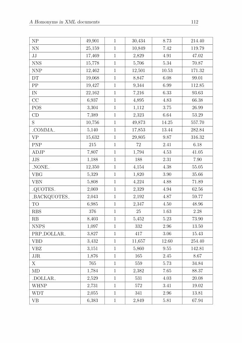
A Homonyms in XML documents 112

NP 49,901 1 30,434 8.73 214.40

NN 25,159 1 10,849 7.42 119.79

JJ 17,469 1 2,829 4.91 47.02

NNS 15,778 1 5,706 5.34 70.87

NNP 12,462 1 12,501 10.53 171.32

DT 19,068 1 8,847 6.08 99.01

PP 19,427 1 9,344 6.99 112.85

IN 22,162 1 7,216 6.33 93.63

CC 6,937 1 4,895 4.83 66.38

POS 3,304 1 1,112 3.75 26.99

CD 7,389 1 2,323 6.64 53.29

S 10,756 1 49,873 14.25 557.70

COMMA 5,140 1 17,853 13.44 282.84

VP 15,632 1 29,805 9.87 316.32

PNP 215 1 72 2.41 6.18

ADJP 7,807 1 1,794 4.53 41.05

JJS 1,188 1 188 2.31 7.90

NONE 12,350 1 4,154 4.38 55.05

VBG 5,329 1 1,820 3.90 35.66

VBN 5,808 1 4,224 4.88 71.89

QUOTES 2,069 1 2,329 4.94 62.56

BACKQUOTES 2,043 1 2,192 4.87 59.77

TO 6,985 1 2,347 4.50 48.96

RBS 376 1 25 1.63 2.28

RB 8,403 1 5,452 5.23 73.90

NNPS 1,097 1 332 2.96 13.50

PRP DOLLAR 3,827 1 417 3.06 15.43

VBD 3,432 1 11,657 12.60 254.40

VBZ 3,151 1 5,860 9.55 142.81

JJR 1,876 1 165 2.45 8.67

X 765 1 559 5.73 34.84

MD 1,784 1 2,382 7.65 88.37

DOLLAR 2,529 1 531 4.03 20.08

WHNP 2,731 1 572 3.41 19.02

WDT 2,055 1 341 2.96 13.81

VB 6,383 1 2,849 5.81 67.94

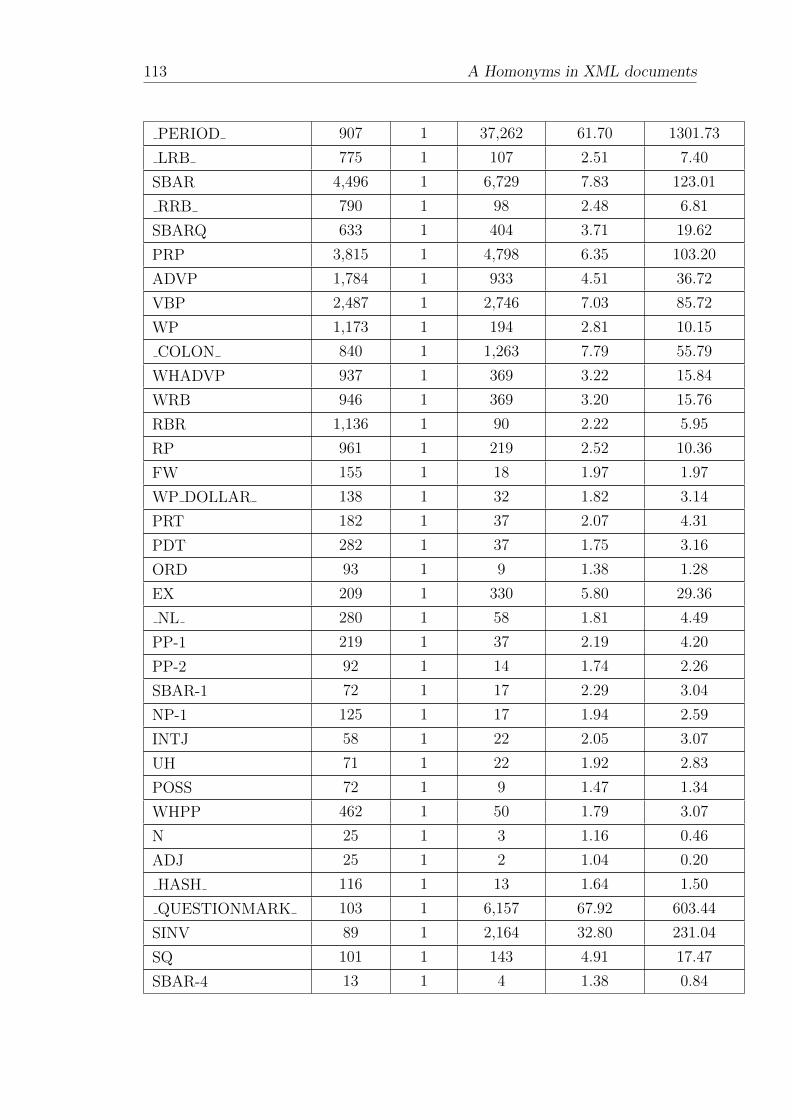
113 A Homonyms in XML documents

PERIOD 907 1 37,262 61.70 1301.73

LRB 775 1 107 2.51 7.40

SBAR 4,496 1 6,729 7.83 123.01

RRB 790 1 98 2.48 6.81

SBARQ 633 1 404 3.71 19.62

PRP 3,815 1 4,798 6.35 103.20

ADVP 1,784 1 933 4.51 36.72

VBP 2,487 1 2,746 7.03 85.72

WP 1,173 1 194 2.81 10.15

COLON 840 1 1,263 7.79 55.79

WHADVP 937 1 369 3.22 15.84

WRB 946 1 369 3.20 15.76

RBR 1,136 1 90 2.22 5.95

RP 961 1 219 2.52 10.36

FW 155 1 18 1.97 1.97

WP DOLLAR 138 1 32 1.82 3.14

PRT 182 1 37 2.07 4.31

PDT 282 1 37 1.75 3.16

ORD 93 1 9 1.38 1.28

EX 209 1 330 5.80 29.36

NL 280 1 58 1.81 4.49

PP-1 219 1 37 2.19 4.20

PP-2 92 1 14 1.74 2.26

SBAR-1 72 1 17 2.29 3.04

NP-1 125 1 17 1.94 2.59

INTJ 58 1 22 2.05 3.07

UH 71 1 22 1.92 2.83

POSS 72 1 9 1.47 1.34

WHPP 462 1 50 1.79 3.07

N 25 1 3 1.16 0.46

ADJ 25 1 2 1.04 0.20

HASH 116 1 13 1.64 1.50

QUESTIONMARK 103 1 6,157 67.92 603.44

SINV 89 1 2,164 32.80 231.04

SQ 101 1 143 4.91 17.47

SBAR-4 13 1 4 1.38 0.84

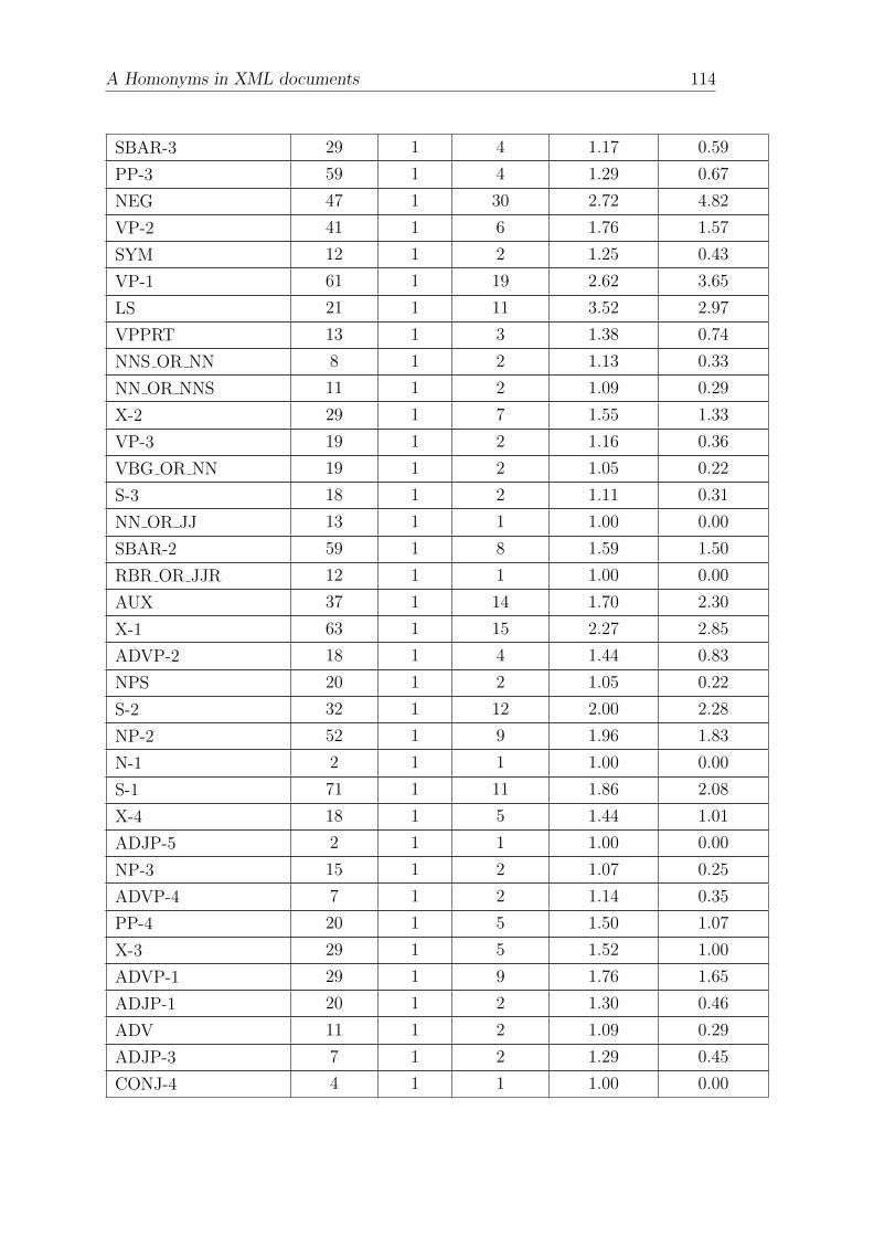
A Homonyms in XML documents 114

SBAR-3 29 1 4 1.17 0.59

PP-3 59 1 4 1.29 0.67

NEG 47 1 30 2.72 4.82

VP-2 41 1 6 1.76 1.57

SYM 12 1 2 1.25 0.43

VP-1 61 1 19 2.62 3.65

LS 21 1 11 3.52 2.97

VPPRT 13 1 3 1.38 0.74

NNS OR NN 8 1 2 1.13 0.33

NN OR NNS 11 1 2 1.09 0.29

X-2 29 1 7 1.55 1.33

VP-3 19 1 2 1.16 0.36

VBG OR NN 19 1 2 1.05 0.22

S-3 18 1 2 1.11 0.31

NN OR JJ 13 1 1 1.00 0.00

SBAR-2 59 1 8 1.59 1.50

RBR OR JJR 12 1 1 1.00 0.00

AUX 37 1 14 1.70 2.30

X-1 63 1 15 2.27 2.85

ADVP-2 18 1 4 1.44 0.83

NPS 20 1 2 1.05 0.22

S-2 32 1 12 2.00 2.28

NP-2 52 1 9 1.96 1.83

N-1 2 1 1 1.00 0.00

S-1 71 1 11 1.86 2.08

X-4 18 1 5 1.44 1.01

ADJP-5 2 1 1 1.00 0.00

NP-3 15 1 2 1.07 0.25

ADVP-4 7 1 2 1.14 0.35

PP-4 20 1 5 1.50 1.07

X-3 29 1 5 1.52 1.00

ADVP-1 29 1 9 1.76 1.65

ADJP-1 20 1 2 1.30 0.46

ADV 11 1 2 1.09 0.29

ADJP-3 7 1 2 1.29 0.45

CONJ-4 4 1 1 1.00 0.00

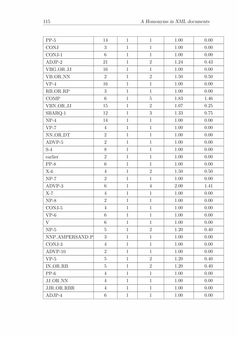
115 A Homonyms in XML documents

PP-5 14 1 1 1.00 0.00

CONJ 3 1 1 1.00 0.00

CONJ-1 6 1 1 1.00 0.00

ADJP-2 21 1 2 1.24 0.43

VBG OR JJ 16 1 1 1.00 0.00

VB OR NN 2 1 2 1.50 0.50

VP-4 16 1 1 1.00 0.00

RB OR RP 3 1 1 1.00 0.00

COMP 6 1 5 1.83 1.46

VBN OR JJ 15 1 2 1.07 0.25

SBARQ-1 12 1 3 1.33 0.75

NP-4 14 1 1 1.00 0.00

VP-7 4 1 1 1.00 0.00

NN OR DT 2 1 1 1.00 0.00

ADVP-5 2 1 1 1.00 0.00

S-4 8 1 1 1.00 0.00

earlier 2 1 1 1.00 0.00

PP-8 6 1 1 1.00 0.00

X-6 4 1 2 1.50 0.50

NP-7 2 1 1 1.00 0.00

ADVP-3 6 1 4 2.00 1.41

X-7 4 1 1 1.00 0.00

NP-8 2 1 1 1.00 0.00

CONJ-5 4 1 1 1.00 0.00

VP-6 6 1 1 1.00 0.00

V 6 1 1 1.00 0.00

NP-5 5 1 2 1.20 0.40

NNP AMPERSAND P 3 1 1 1.00 0.00

CONJ-3 4 1 1 1.00 0.00

ADVP-10 2 1 1 1.00 0.00

VP-5 5 1 2 1.20 0.40

IN OR RB 5 1 2 1.20 0.40

PP-6 4 1 1 1.00 0.00

JJ OR NN 4 1 1 1.00 0.00

JJR OR RBR 4 1 1 1.00 0.00

ADJP-4 6 1 1 1.00 0.00

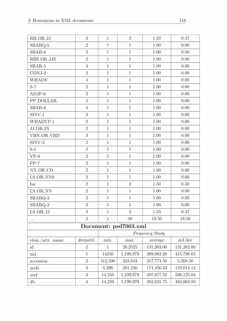
A Homonyms in XML documents 116

RB OR JJ 3 1 2 1.33 0.47

SBARQ-5 2 1 1 1.00 0.00

SBAR-8 2 1 1 1.00 0.00

RBS OR JJS 2 1 1 1.00 0.00

SBAR-5 4 1 1 1.00 0.00

CONJ-2 2 1 1 1.00 0.00

WHADV 4 1 1 1.00 0.00

S-7 2 1 1 1.00 0.00

ADJP-6 2 1 1 1.00 0.00

PP DOLLAR 2 1 1 1.00 0.00

SBAR-6 4 1 1 1.00 0.00

SINV-1 3 1 1 1.00 0.00

WHADVP-1 2 1 1 1.00 0.00

JJ OR IN 2 1 1 1.00 0.00

VBN OR VBD 3 1 1 1.00 0.00

SINV-3 2 1 1 1.00 0.00

S-5 2 1 1 1.00 0.00

VP-8 2 1 1 1.00 0.00

PP-7 2 1 1 1.00 0.00

NN OR CD 2 1 1 1.00 0.00

LS OR NNS 2 1 1 1.00 0.00

Inc 2 1 2 1.50 0.50

LS OR NN 2 1 1 1.00 0.00

SBARQ-3 2 1 1 1.00 0.00

SBARQ-2 2 1 1 1.00 0.00

LS OR JJ 3 1 2 1.33 0.47

2 1 38 19.50 18.50

Document: psd7003.xmlFrequency Study

elem./attr. name #repetit. min. max. average std.dev

id 2 1 26,2525 131,263.00 131,262.00

uid 5 14250 1,199,979 389,883.20 415,798.65

accession 2 312,506 323,043 317,774.50 5,268.50

xrefs 3 8,396 281,246 174,456.33 119,014.12

xref 3 14,250 1,199,979 497,877.33 508,125.04

db 4 14,250 1,199,979 382,831.75 483,062.89

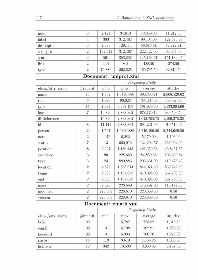
117 A Homonyms in XML documents

note 5 2,124 34,640 13,359.80 11,212.35

label 4 383 312,467 99,404.00 127,583.68

description 3 7,683 129,114 56,676.67 52,272.21

seq-spec 2 132,377 312,467 222,422.00 90,045.00

status 3 501 353,838 145,163.67 151,183.95

link 2 114 863 488.50 374.50

type 2 76,886 262,525 169,705.50 92,819.50

Document: uniprot.xmlFrequency Study

elem./attr. name #repetit. min. max. average std.dev

name 14 1,507 1,0490,886 890,360.71 2,668,529.62

ref 5 1,086 90,028 384,11.40 390,92.59

type 15 7,994 3,937,497 791,989.60 1,133,994.60

key 7 16,840 2,833,362 678,179.14 930,590.56

dbReference 4 16,840 2,833,362 1,012,795.75 1,109,378.38

id 8 11,114 2,833,362 694,221.00 910,510.44

person 2 1,507 1,0490,886 5,246,196.50 5,244,689.50

note 2 4,076 6,282 5,179.00 1,103.00

status 7 13 660,912 134,294.57 233,004.00

position 8 2,207 1,136,443 421,659.63 46,8457.35

sequence 3 90 228,669 84,859.33 102,229.84

text 3 23 889,886 296,661.00 419,473.42

location 2 4,829 1,683,314 844,071.50 839,242.50

begin 2 2,338 1,137,858 570,098.00 567,760.00

end 2 2,338 1,137,858 570,098.00 567,760.00

mass 2 2,325 228,669 115,497.00 113,172.00

modified 2 228,669 228,670 228,669.50 0.50

version 2 228,669 228,670 228,669.50 0.50

Document: xmark.xmlFrequency Study

elem./attr. name #repetit. min. max. average std.dev

bold 99 11 5,787 725.82 1,315.59

emph 99 4 5,798 702.91 1,280.63

keyword 99 4 5,933 706.76 1,279.09

parlist 18 119 3,619 1,156.28 1,088.60

listitem 18 342 10,533 3,360.06 3,157.86

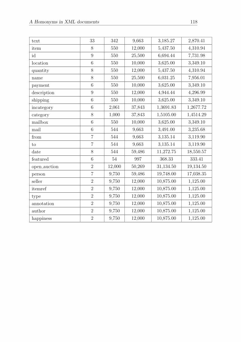
A Homonyms in XML documents 118

text 33 342 9,663 3,185.27 2,870.41

item 8 550 12,000 5,437.50 4,310.94

id 9 550 25,500 6,694.44 7,731.98

location 6 550 10,000 3,625.00 3,349.10

quantity 8 550 12,000 5,437.50 4,310.94

name 8 550 25,500 6,031.25 7,956.01

payment 6 550 10,000 3,625.00 3,349.10

description 9 550 12,000 4,944.44 4,296.99

shipping 6 550 10,000 3,625.00 3,349.10

incategory 6 2,061 37,843 1,3691.83 1,2677.72

category 8 1,000 37,843 1,5105.00 1,4514.29

mailbox 6 550 10,000 3,625.00 3,349.10

mail 6 544 9,663 3,491.00 3,235.68

from 7 544 9,663 3,135.14 3,119.90

to 7 544 9,663 3,135.14 3,119.90

date 8 544 59,486 11,272.75 18,550.57

featured 6 54 997 368.33 333.41

open auction 2 12,000 50,269 31,134.50 19,134.50

person 7 9,750 59,486 19,748.00 17,038.35

seller 2 9,750 12,000 10,875.00 1,125.00

itemref 2 9,750 12,000 10,875.00 1,125.00

type 2 9,750 12,000 10,875.00 1,125.00

annotation 2 9,750 12,000 10,875.00 1,125.00

author 2 9,750 12,000 10,875.00 1,125.00

happiness 2 9,750 12,000 10,875.00 1,125.00

Bibliography

[AAN01] Ashraf Aboulnaga, Alaa R. Alameldeen, and Jeffrey F. Naughton.

Estimating the selectivity of XML path expressions for internet scale

applications. In Proc. VLDB Conference, pages 591–600, 2001.

[AKJP+02] Shurug Al-Khalifa, H. V. Jagadish, Jignesh M. Patel, Yuqing Wu,

Nick Koudas, and Divesh Srivastava. Structural joins: A primitive

for efficient XML query pattern matching. In ICDE ’02: Proceedings

of the 18th International Conference on Data Engineering, pages 141–

154, Washington, DC, USA, 2002. IEEE Computer Society.

[AMFH08a] Jose de Aguiar Moraes Filho and Theo Harder. Accurate histogram-

based XML summarization. In Proc. SAC, pages 998–1002, 2008.

[AMFH08b] Jose de Aguiar Moraes Filho and Theo Harder. EXsum—an XML

summarization framework. In Proc. IDEAS, pages 139–148, 2008.

[AMFH08c] Jose de Aguiar Moraes Filho and Theo Harder. Tailor-made XML

synopses. In Proceedings of the Eighth International Baltic Confer-

ence — BalticDB&IS 2008, pages 25–36, 2008.

[AMFHS09] Jose de Aguiar Moraes Filho, Theo Harder, and Caetano Sauer. En-

hanced statistics for element-centered XML summaries. In D. Slezak,

T.-H. Kim, Y. Zhang, J. Ma, and K.-I. Chung, editors, Proceedings

of the International Database Theory and Applications Conference —

DTA 2009, volume 64 of Communications in Computer and Informa-

tion Science–LNCS Series, pages 99–106. Springer, 2009.

[BHH09] Sebastian Bachle, Theo Harder, and Michael Peter Haustein. Im-

plementing and optimizing fine-granular lock management for XML

document trees. In Xiaofang Zhou, Haruo Yokota, Ke Deng, and

Qing Liu, editors, DASFAA, volume 5463 of Lecture Notes in Com-

puter Science, pages 631–645. Springer, 2009.

119

Bibliography 120

[BKS02] Nicolas Bruno, Nick Koudas, and Divesh Srivastava. Holistic twig

joins: optimal XML pattern matching. In SIGMOD ’02: Proceedings

of the 2002 ACM SIGMOD international conference on Management

of data, pages 310–321, New York, NY, USA, 2002. ACM.

[Blo70] Burton H. Bloom. Space/time trade-offs in hash coding with allow-

able errors. Commun. ACM, 13(7):422–426, 1970.

[BLS07] Sourav S. Bhowmick, Erwin Leonardi, and Hongmei Sun. Efficient

evaluation of high-selective XML twig patterns with parent child

edges in tree-unaware rdbms. In CIKM ’07: Proceedings of the six-

teenth ACM conference on Conference on information and knowledge

management, pages 673–682, New York, NY, USA, 2007. ACM.

[CGG04] Surajit Chaudhuri, Venkatesh Ganti, and Luis Gravano. Selectivity

estimation for string predicates: Overcoming the underestimation

problem. In ICDE, pages 227–238. IEEE Computer Society, 2004.

[Cod83] Edgar F. Codd. A relational model of data for large shared data

banks. Commun. ACM, 26(1):64–69, 1983.

[Cod90] Edgar F. Codd. The relational model for database management: ver-

sion 2. Addison-Wesley Longman Publishing Co., Inc., Boston, MA,

USA, 1990.

[DJL91] Ronald A. DeVore, Bjorn D. Jawerth, and Bradley J. Lucier. Data

compression using wavelets: Errors, smoothness, and quantization.

In Data Compression Conference, pages 186–195, 1991.

[FHR+02] Juliana Freire, Jayant R. Haritsa, Maya Ramanath, Prasan Roy, and

Jerome Simeon. Statix: making XML count. In SIGMOD Confer-

ence, pages 181–191, 2002.

[FJSY05] Marcus Fontoura, Vanja Josifovski, Eugene Shekita, and Beverly

Yang. Optimizing cursor movement in holistic twig joins. In CIKM

’05: Proceedings of the 14th ACM international conference on Infor-

mation and knowledge management, pages 784–791, New York, NY,

USA, 2005. ACM.

[GW97] Roy Goldman and Jennifer Widom. Dataguides: Enabling Query

Formulation and Optimization in Semistructured Databases. In Proc.

VLDB Conference, pages 436–445, 1997.

Bibliography BIBLIOGRAPHY

[Har96] Theo Harder. Datenstrukturen – Beispiele in MODULA-2 (German

only). TU Kaiserslautern, 1996.

[HMS07] Theo Harder, Christian Mathis, and Karsten Schmidt. Comparison

of complete and elementless native storage of XML documents. In

IDEAS, pages 102–113. IEEE Computer Society, 2007.

[Ioa03] Yannis E. Ioannidis. The history of histograms (abridged). In VLDB,

pages 19–30, 2003.

[IP95] Yannis E. Ioannidis and Viswanath Poosala. Balancing histogram op-

timality and practicality for query result size estimation. In Michael J.

Carey and Donovan A. Schneider, editors, SIGMOD Conference,

pages 233–244. ACM Press, 1995.

[JKM+02] Jouko Jantti, Henry Kiesslich, Roddy Munro, John Schlatweiler, and

Bill Stillwell. IMS Version 8 Implementation Guide A Technical

Overview of the New Features. IBM Red Books, 2002.

[JLST02] H. V. Jagadish, Laks V. S. Lakshmanan, Divesh Srivastava, and Keith

Thompson. Tax: A tree algebra for XML. In DBPL ’01: Revised Pa-

pers from the 8th International Workshop on Database Programming

Languages, pages 149–164, London, UK, 2002. Springer-Verlag.

[JLW04] Haifeng Jiang, Hongjun Lu, and Wei Wang. Efficient processing of

XML twig queries with or-predicates. In SIGMOD ’04: Proceedings

of the 2004 ACM SIGMOD international conference on Management

of data, pages 59–70, New York, NY, USA, 2004. ACM.

[JWLY03] Haifeng Jiang, Wei Wang, Hongjun Lu, and Jeffrey Xu Yu. Holistic

twig joins on indexed XML documents. In VLDB ’2003: Proceedings

of the 29th international conference on Very large data bases, pages

273–284. VLDB Endowment, 2003.

[Kep04] Stephan Kepser. A simple proof for the turing-completeness of xslt

and xquery. In Extreme Markup Languages, 2004.

[LCL04] Jiaheng Lu, Ting Chen, and Tok Wang Ling. Efficient processing of

XML twig patterns with parent child edges: a look-ahead approach.

In CIKM ’04: Proceedings of the thirteenth ACM international con-

ference on Information and knowledge management, pages 533–542,

New York, NY, USA, 2004. ACM.

Bibliography 122

[LHH00] Rick Long, Robert Hain, and Mark Harrington. IMS Primer. IBM

Red Books, 2000.

[LWP+02] Lipyeow Lim, Min Wang, Sriram Padmanabhan, Jeffrey Scott Vit-

ter, and Ronald Parr. Xpathlearner: An on-line self-tuning markov

histogram for XML path selectivity estimation. In Proc. VLDB Con-

ference, pages 442–453, 2002.

[Mat07] Christian Mathis. Extending a tuple-based xpath algebra to en-

hance evaluation flexibility. Informatik - Forschung und Entwicklung,

21(3):147–164, June 2007.

[MCS88] Michael V. Mannino, Paicheng Chu, and Thomas Sager. Statisti-

cal profile estimation in database systems. ACM Comput. Surv.,

20(3):191–221, 1988.

[MHH06] Christian Mathis, Theo Harder, and Michael Haustein. Locking-

aware structural join operators for XML query processing. In SIG-

MOD ’06: Proceedings of the 2006 ACM SIGMOD international con-

ference on Management of data, pages 467–478, New York, NY, USA,

2006. ACM.

[MHM03] Norman May, Sven Helmer, and Guido Moerkotte. Three cases

for query decorrelation in xquery. In Zohra Bellahsene, Akmal B.

Chaudhri, Erhard Rahm, Michael Rys, and Rainer Unland, editors,

Xsym, volume 2824 of Lecture Notes in Computer Science, pages 70–

84. Springer, 2003.

[NZ06] Leonid Novak and Alexandre V. Zamulin. An XML algebra for

xquery. In Yannis Manolopoulos, Jaroslav Pokorny, and Timos K.

Sellis, editors, ADBIS, volume 4152 of Lecture Notes in Computer

Science, pages 4–21. Springer, 2006.

[Oll78] T. William Olle. The Codasyl Approach to Data Base Management.

John Wiley & Sons, Inc., New York, NY, USA, 1978.

[PG02] Neoklis Polyzotis and Minos N. Garofalakis. Structure and value

synopses for XML data graphs. In Proc. VLDB Conference, pages

466–477, 2002.

[PG06] Neoklis Polyzotis and Minos N. Garofalakis. Xsketch synopses for

XML data graphs. ACM Trans. Database Syst., 31(3):1014–1063,

2006.

Bibliography BIBLIOGRAPHY

[PHIS96] Viswanath Poosala, Peter J. Haas, Yannis E. Ioannidis, and Eugene J.

Shekita. Improved histograms for selectivity estimation of range pred-

icates. SIGMOD Rec., 25(2):294–305, 1996.

[PSC84] Gregory Piatetsky-Shapiro and Charles Connell. Accurate estimation

of the number of tuples satisfying a condition. In Beatrice Yormark,

editor, SIGMOD Conference, pages 256–276. ACM Press, 1984.

[SA02] Carlo Sartiani and Antonio Albano. Yet another query algebra for

XML data. International Database Engineering and Applications

Symposium, 0:106, 2002.

[SH07] Karsten Schmidt and Theo Harder. Tailor-made native XML stor-

age structures. In Yannis E. Ioannidis, Boris Novikov, and Boris

Rachev, editors, ADBIS Research Communications, volume 325 of

CEUR Workshop Proceedings. CEUR-WS.org, 2007.

[TF76] Robert W. Taylor and Randall L. Frank. Codasyl data-base manage-

ment systems. ACM Comput. Surv., 8(1):67–103, 1976.

[W3C98] W3C. Document object model (DOM) level 1 specification version

1.0 — W3C recommendation — 1 october, 1998. http://www.w3.

org/TR/1998/REC-DOM-Level-1-19981001/, 1998.

[W3C06] W3C. Extensible markup language (XML) 1.1 (second edition) —

W3C recommendation — 16 august 2006, edited in place 29 septem-

ber 2006. http://www.w3.org/TR/2006/REC-xml11-20060816/,

2006.

[W3C07] W3C. XML path language (xpath) 2.0 — W3C recommendation —

23 january 2007. http://www.w3.org/TR/xpath20/, 2007.

[W3C08] W3C. XML schema definition language (xsd) 1.1 part 2: Datatypes

— W3C working draft — 20 june 2008. http://www.w3.org/TR/

xmlschema11-2/, 2008.

[WH09] Andreas M. Weiner and Theo Harder. Using structural joins and

holistic twig joins for native XML query optimization. In Paolo

Atzeni, Albertas Caplinskas, and Hannu Jaakkola, editors, ADBIS,

volume 5207 of Lecture Notes in Computer Science, pages 2–13.

Springer, 2009.

124

[WJLY04] Wei Wang, Haifeng Jiang, Hongjun Lu, and Jeffrey Xu Yu. Bloom

histogram: Path selectivity estimation for XML data with updates.

In Proc. VLDB Conference, pages 240–251, 2004.

[WPJ03] Yuqing Wu, Jignesh M. Patel, and H. V. Jagadish. Structural join or-

der selection for XML query optimization. International Conference

on Data Engineering, 0:443–454, 2003.

[ZOAI06] Ning Zhang, M. Tamer Ozsu, Ashraf Aboulnaga, and Ihab F. Ilyas.

Xseed: Accurate and fast cardinality estimation for xpath queries. In

Proc. ICDE, page 61, 2006.

[ZPR02] Xin Zhang, Bradford Pielech, and Elke A. Rundesnteiner. Honey,

i shrunk the xquery!: an XML algebra optimization approach. In

WIDM ’02: Proceedings of the 4th international workshop on Web in-

formation and data management, pages 15–22, New York, NY, USA,

2002. ACM.

Curriculum Vitae

Jose de Aguiar Moraes Filho

Personal Data:

Business Address: Paul-Ehrlich-Str. 36 R. 315

67663 Kaiserslautern

Germany

Phone: +49 (0) 631 205 3271

Email: aguiar@cs.uni-kl.de

Date of Bith: September 4th 1966

Place of Birth: Fortaleza, Ceara, Brazil

Marital Status: Married

Nationality: Brazilian

Education and Work Experience:

01/2006 – 12/2009 Doctoral Candidate at University of Kaiserslautern

(Databases and Information Systems Workgroup)

10/2003 – 12/2005 Assistant Professor at University of Fortaleza (UNIFOR)

Lectures: Fundamentals of Database Systems and

Database Implementation Techniques

Database Administrator at SERPRO

01/2001 – 09/2003 Graduate Studies at University of Fortaleza (UNIFOR)

Academic Degree: Master in Applied Informatics

Main Focus: Databases and Information Systems

Minor Subject: Mobile Databases

Master Dissertation: AMDB – An Approach for Sharing Mobile Databases

01/1988 – 12/2000 Professional Activities in Companies:

SERPRO (Brazilian Federal Government Data Center) – until now,

UNIMED (Health Insurance Provider and Medical Cooperative),

Banking System – in state and private institutions,

125

126

ABC Bull Telematic (joint-venture with Honeywell-Bull),

and Teleceara (State Telecom company)

The activities varied from:

support analyst (ABC Bull and UNIMED),

database administrator (UNIMED and SERPRO),

system analyst and developer (Teleceara and UNIMED),

consulting (Banking System),

and professional training (scattered throughout this period).

06/1992 – 06/1993 Assistant Professor at University of Fortaleza (UNIFOR)

Lectures: Teleprocessing and Computer Networks

01/1984 – 12/1987 Undergraduate Studies at State University of Ceara

Bachelor degree

01/1981 – 12/1983 Secondary School: “Farias Brito”