Summer 2012 Calculus I Lecture Notes

CALCULUS MATH 165 FALL 2016 (COHEN) LECTURE NOTES

Remark 0.1. Much of this set of lecture notes is adapted from a combination of Rogawski’s CalculusEarly Transcendentals and Briggs’ and Cochran’s Calculus, and many of the examples used appearpreviously in these texts.

1 Vague History, and Motivation From Physics

Remark 1.1 (History of the Calculus). Most students tend to define calculus as “derivatives and in-tegrals,” and credit Isaac Newton and Gottfriend Wilhelm Leibniz with its “discovery” in the late 17thcentury. This viewpoint is not wholly incorrect, but reductive—the calculus actually has a long andcomplicated history which in many ways predates Newton and Leibniz, even as far back as the philo-sophical questions about “infinitely small distances” posed by ancient Greeks, and which developed farbeyond the 17th century techniques. Broadly, calculus can be regarded as a collection of techniques forsolving a variety of very different but related types of problems, such as: What is the slope of a tangentline to a curve? (differential calculus) What is the area under a curve? (integral calculus) How long is acurve? What is the volume of a body in space? What is the sum of infinitely many real numbers? andmany others.

The standard solutions to these diverse types of problems are tied together by the notion of a limit,which we will spend the first few weeks of the course defining and studying. A limit in calculus is a fairlymodern notion, which replaced previous concepts like infinitesimals, Newton’s fluxions and Leibniz’sdifferentials. These older notions proved problematic in establishing a rigorous theory for the calculus,although they still rear their head sometimes in the notation. (More on this later—see Remark 8.9 forinstance.)

Newton and Leibniz deserve credit for giving a systematic treatment to the class of problems listedabove, thus “inventing” the calculus. But our modern treatment owes a huge amount to Fermat, Euler,Lagrange, Gauss, Cauchy, Weierstrass, and too many others to list here.

To see how the fundamental notion of a limit might arise naturally, we consider the simple physicsproblem posed below.

Example 1.2. A ball is launched into the air at 96 ft/s. Gravity accelerates the ball downward at arate of 32 ft/s. The height of the ball in feet after t seconds is given by the function:

h(t) = −16t2 + 96t

Question 1: How long until the ball lands?

By setting h(t) = 0 and solving for t, we see that the height of the ball is 0 feet after exactly 6 seconds.

Question 2: How high does the ball go?

The graph of h(t) is a parabola and hence symmetrical about some vertex. Since the ball has height0 at t = 0 and t = 6, its vertex must lie directly between, at t = 3. Then its maximum height is givenby h(3) = 144 feet.

Question 3: What is the average velocity of the ball in the first 3 seconds?

The ball goes up 144 feet in 3 seconds, so its average velocity is 1443 = 48 ft/s.

1

2 CALCULUS MATH 165 FALL 2016 (COHEN) LECTURE NOTES

Question 4: What is the average velocity of the ball from t = 1 to t = 3 seconds?

Velocity should be given by distance/time. The ball’s height changes from h(1) feet to h(3) feetbetween t = 1 and t = 3. So its average velocity over this interval is given by:

h(3)− h(1)

3− 1=

144− 80

3− 1= 32 ft/s.

The formula above should recall the slope formula m = y2−y1x2−x1

learned in College Algebra. Indeed,the average velocity from any t = 1 to t = 3 is exactly the slope of the line passing through the points(1, h(1)) and (3, h(3)).

Question 5: Exactly how fast is the ball going at t = 1 second? (Our first calculus question!)

You can get good estimates of this instantaneous velocity by computing the average velocity oververy small intervals around t = 1. For example, we can compute the average velocities for .1, then .01,then .00001 seconds after t = 1, as below:

h(1.1)− h(1)

1.1− 1≈ 62.4 ft/s

h(1.01)− h(1)

1.01− 1≈ 63.8 ft/s

h(1.00001)− h(1)

1.00001− 1≈ 63.9998 ft/s

The problem is that each of the above is just an approximation of the actual velocity at t = 1... but asmathematicians we are truly interested in the exact value! We can get better and better approximationsby examining smaller and smaller intervals, but for our purposes, any positive interval at all will be “toolarge.” To solve this problem, we wish to look at “arbitrarily small distances” on the real number line.

Newton/Leibniz approached this by relying on a notion which we now regard as non-rigorous: aninfinitesimal, that is, a distance which is non-zero, yet “infinitely small,” i.e. smaller than any positivereal number. Many mathematicians in the 18th century and earlier freely used the idea of an infinites-imal in their work. Modern mathematicians, however, regard the notion of an “infinitely small” valueas nebulous in meaning, and we abhor the violation of the Archimedean principle! So, in order to solvecalculus problems rigorously, we need to develop some new technology, in particular the notion of limits,whose formal definition is due in an early form to Bernard Bolzano in 1817, and in its present form toKarl Weierstrass in the second half of the 19th century.

2 Limits

Definition 2.1 (Informal Definition). Let f(x) be a function and a be a real number. If there existssome number L such that f(x) is arbitrarily close to L whenever x is sufficiently close (but not equal)to a, then we write:

limx→a

f(x) = L

and say “the limit of f(x) as x approaches a is L.”

If no such number L exists, then we say the limit does not exist.

Remark 2.2. The student may note that the terms “arbitrarily close” and “sufficiently close” aresomewhat vague. Rest assured, the notion of a limit has a precise and clearly stated mathematicaldefinition! However, this definition is more easily understood after some intuition about limits is alreadydeveloped, so we will omit this formal definition here and present it later after we have done a fewexercises.

CALCULUS MATH 165 FALL 2016 (COHEN) LECTURE NOTES 3

Example 2.3. Let f(x) = x+ 2. Find limx→1

f(x), if the limit exists.

Example 2.4. Let g(x) = x2. Find limx→4

g(x), if the limit exists.

Example 2.5. Graphical example (possibly 2.2 #12).

Example 2.6. Let f(x) =√x−1x−1 . Find lim

x→1f(x), if the limit exists.

Solution. We can try to solve the above problem by making a table of function values where x is veryclose to 1.

x = .9 .09 .009 1.001 1.01 1.1f(x) = .5131670 .5012563 .5001251 .4998750 .4987562 .4880885

It appears that as x gets very close to 1, f(x) gets close to .5, and we guess that limx→1

f(x) = .5. This

will turn out to be correct, but note that at this point in our course we are merely making a conjecture,or educated guess! (How do you know the limit is .5 and not .500000001 or .499999999?)

�

Example 2.7 (A Limit That Does Not Exist). Find limx→0

sinπ

x, if the limit exists.

Example 2.8. Let f(x) = x2−5x+6x−2 . Find lim

x→2f(x), if the limit exists.

Solution. To solve this, we first note that x2 − 5x + 6 = (x − 2)(x − 3) in the numerator of f(x). Ourgut says to divide out the (x − 2) from top and bottom and be done with it! However, it is importantto note that the following equation is NOT true:

(x− 2)(x− 3)

x− 2= x− 3

The reason the above equation is false is because x could take on the value of any real number. Inparticular, if x = 2, then the left side of the equation is undefined, while the right side is equal to −1;so we don’t have true equality here.

However, when we are computing the limit of f(x) as x approaches 2, we restrict our attention toall possible values of x which are near, but not equal to the value 2. This means that, since the aboveequation holds for all x 6= 2, the following equation makes perfect sense:

limx→2

(x− 2)(x− 3)

x− 2= limx→2

x− 3

Since the latter limit is −1, we have limx→2

f(x) = −1. �

Now we will go back and cover our tracks by including the formal definition of a limit.

Definition 2.9 (Formal Definition). Let f(x) be a function and a be a real number. Suppose that f(x)exists for all x in some open interval containing a. We say that the limit of f(x) as x approachesa is L, written lim

x→af(x) = L, if the following statement holds: For any positive number ε > 0, there

exists a corresponding number δ > 0 (depending on ε) such that

|f(x)− L| < ε whenever |x− a| < δ.

Why does the above definition make sense? The definition above should give the student confidencethat the intuitive notion of a limit may be made mathematically precise. Proceeding with such assur-ances, all future limit definitions will be presented in the informal style.


Definition 2.10. The left-hand limit: If f(x) is arbitrarily close to L for all x sufficiently closeto a, with x < a, then we say ”the limit of f(x) as x approaches a from the left is L,” and write:limx→a−

f(x) = L.

Definition 2.11. The right-hand limit: If f(x) is arbitrarily close to L for all x sufficiently closeto a, with x > a, then we say ”the limit of f(x) as x approaches a from the right is L,” and write:limx→a+

f(x) = L.

Example 2.12. Graphical example where left- and right-hand limits are not equal.

Fact 2.13. limx→

f(x) = L if and only if limx→a−

f(x) = limx→a+

= L.

3 Continuity

Definition 3.1. We say that a function f is continuous at a point a if the following all hold:

(1) f(a) is defined.

(2) limx→a

f(x) exists.

(3) limx→a

f(x) = f(a).

If f is continuous at every real number, then we say that f is continuous.

Example 3.2. (1) Linear functions (y = mx+ b) are continuous.

(2) Polynomials are continuous.

(3) Rational functions, or functions of the form p(x)q(x) , where p(x) and q(x) are polynomials, are con-

tinuous at every point except where q(x) = 0.

(4) Sine and cosine are continuous everywhere. The tangent function is continuous everywhereexcept points of the form π

2 + kπ, where k is any integer.(5) Exponential functions (y = bx for some positive real number b) are continuous everywhere.

Logarithms are continuous everywhere they are defined.

Remark 3.3 (The Significance of Continuity For Evaluating Limits). If a function is continuous at apoint a, then by definition lim

x→af(x) = f(a). This means to evaluate a continuous function’s limit at a,

you can just plug a into the function!

Example 3.4. Find the limits, if they exist:

(1) limx→3

f(x), where f(x) = 12x− 7

(2) limx→−1

(5x4 − πx3 − 1)

(3) limx→5

g(x), where g(x) = 6

(4) limx→1

x2 − 6x+ 8

x2 − 9

Solution. For part (1), simply observe that f(x) is a linear function and hence continuous. In that case,

limx→3

f(x) = f(3) =1

2· 3− 7 = −11

2. The remaining problems are solved similarly. �

Theorem 3.5 (Intermediate Value Theorem). If f is a continuous function on a closed interval [a, b],then for every value M between f(a) and f(b), there exists at least one c ∈ (a, b) such that f(c) = M .

Example 3.6. Prove that the equation sinx = 0.3 has at least one solution.


Fact 3.7. Suppose limx→a

f(x) and limx→a

g(x) exist. Suppose c is a real number, and m,n > 0 are integers.

The following all hold:

(1) limx→a

[f(x) + g(x)] = limx→a

f(x) + limx→a

g(x)

(2) limx→a

[cf(x)] = c[ limx→a

f(x)]

(3) limx→a

[f(x)g(x)] = [ limx→a

f(x)][ limx→a

g(x)]

(4) limx→a

f(x)

g(x)=

limx→a f(x)

limx→a g(x), provided lim

x→ag(x) 6= 0.

(5) limx→a

[f(x)]nm = [ lim

x→af(x)]

nm , provided f(x) ≥ 0 for x near a if m is even and n

m is in reduced

form.

Example 3.8. Compute limx→1

√x− 1

x− 1, if it exists.

Solution. Recall: when we tackled this problem earlier using a table, we conjectured that the limit is12 = .5. We will now show that our conjecture was correct by observing the following:

limx→1

√x− 1

x− 1= limx→1

√x− 1

(√x− 1)(

√x+ 1)

= limx→1

1√x+ 1

(Note that we may cancel to obtain the second equality, since we are taking a limit.) Now since1√x+ 1

is continuous at x = 1, we may substitute to finish the problem.

limx→1

√x− 1

x− 1= limx→1

1√x+ 1

=1√

1 + 1=

1

2.

�

4 Infinite Limits

Example 4.1. Find limx→0

1

x2, if it exists.

Solution. Note that if we take x to be a very small number (i.e. close to 0), then x2 will be an evensmaller POSITIVE number. Then its reciprocal 1

x2 will be a very large positive number. In fact, the

smaller we take x to be, the larger the value of 1x2 will be, i.e. the function 1

x2 becomes arbitrarily largeas x approaches 0.

By our previous definition of limits, there is no number L which 1x2 approaches when x → 0, so we

say that the limit does not exist. However, we wish to describe this kind of phenomenon in functions,so we will now expand our definition suitably. �

Definition 4.2. Let f(x) be a function and a a real number. If f(x) grows arbitrarily large for xsufficiently close to a, then we write lim

x→af(x) =∞.

Similarly, if f(x) grows arbitrarily large in magnitude but in the negative direction, then we writelimx→a

f(x) = −∞.

We can also define the one-sided limits limx→a−

f(x) and limx→a+

f(x) to be∞ or −∞, in the analogous way.

Example 4.3. Graphical example.


Example 4.4. Find (a) limx→π

2−

tanx and (b) limx→π

2+

tanx, if they exist.

Solution. A quick sketch of the graph of the tangent function shows that limx→π

2−

tanx =∞ and limx→π

2+

tanx =

−∞. �


5 + x

x, if it exists.

Solution. Taking x to be a very small positive number, we observe that 5 +x will be very close to 5, and

hence we can approximate5 + x

x≈ 5

x. The latter fraction will grow arbitrarily large as x approaches 0

from the right, so we have limx→0+

5 + x

x=∞.

On the other hand, if we take x to be a very small negative number, then we still have 5 + x ≈ 5 and

hence5 + x

x≈ 5

x. This time, however, the latter fraction will grow arbitrarily large in magnitude in

the negative direction, since a positive number divided by a negative number is negative. This implies

limx→0−

5 + x

x= −∞.

Since this function has two different one-sided limits, we say that the limit does not exist. �

Remark 4.6. The lesson we take from the above example is that for functions of the formp(x)

q(x), if p(x)

stays relatively constant but q(x) goes to 0 as x → a, thenp(x)

q(x)will blow up in either the positive or

negative direction. Whether the limit is ∞, −∞, or does not exist will depend on the signs of p(x) andq(x) when x is near a.

Example 4.7. Find (a) limx→3+

2− 5x

x− 3and (b) lim

x→3−

2− 5x

x− 3, if they exist.

5 Limits at Infinity

Definition 5.1. If f(x) becomes arbitrarily close to L for all sufficiently large and positive x, we writelimx→∞

f(x) = L.

If f(x) becomes arbitrarily close to L for all sufficiently large and negative X, then we write limx→−∞

f(x) =

L.

Example 5.2. Let f(x) =x√

x2 + 1. Find lim

x→∞f(x), if it exists.

Example 5.3. Find limx→−∞

(2 +10

x2), if it exists.

Example 5.4. Find limx→∞

(2x+ 8), if it exists.

Remark 5.5 (End Behavior of Polynomials). The previous example shows that it makes sense to com-bine infinite limits and limits at infinity, when appropriate.

We can also use limits at infinity to characterize the end behavior of functions. The student may recallfrom a previous algebra course that for polynomial functions f(x) = anx

n+an−1xn−1+...+a2x

2+a1x+a0,the end behavior of f(x) is determined entirely by the first term anx

n, according to the following rules:

If n is even and an is positive, then limx→−∞

f(x) = limx→∞

f(x) =∞.

If n is even and an is negative, then limx→−∞

f(x) = limx→∞

f(x) = −∞.


If n is odd and an is positive, then limx→−∞

f(x) = −∞ and limx→∞

f(x) =∞.

If n is odd and an is negative, then limx→−∞

f(x) =∞ and limx→∞

f(x) = −∞.

Now let us consider the limits at infinity of rational functions, i.e. fractions of polynomials.

6 Indeterminate Forms, and End Behavior of Rational Functions

Definition 6.1 (Informal Definition). We say that the limit limx→a

f(x) is of indeterminate form if the

initial attempt to evaluate f(c) yields an undefined expression of the type 00 , ∞∞ , ∞ · 0, or ∞−∞.

Example 6.2. Observe that the following limits are of indeterminate form, and try to evaluate them.

(1) limx→3

x2 − 4x+ 3

x2 + x− 12

(2) limx→π/2−

tanx

secx

(3) limx→1+

(1

x− 1− 2

x2 − 1

)(4) lim

x→0x lnx

Example 6.3. Find the following limits if they exist.

(1) limx→∞

12x− 7

x3 + 1

(2) limx→∞

5x5 − 4x2 + 2

2x4 − πx2 + 6x− 1

(3) limx→∞

3x7 − 22x5 + 19x

8x7 − 100x6 + 22

Fact 6.4 (Limits at Infinity for Rational Functions). Suppose f(x) is a rational function, i.e.

f(x) =axn + ...

bxm + ...

for some nonnegative integers n and m and some non-zero leading coefficients a and b. (Here the ellipsison the numerator represents terms of degree less than n, and the ellipsis on the denominator representsterms of degree less than m.) Then the following hold:

(1) If n < m, then limx→∞

f(x) = 0.

(2) If n > m, then limx→∞

f(x) =∞.

(3) If n = m, then limx→∞

f(x) =a

b.

Remark 6.5. The previous rule takes care of limits at positive infinity for all rational functions, whatabout limits at negative infinity? A very similar rule should apply for determining lim

x→−∞f(x), where f

is a rational function, but it needs to depend on whether n and m are even or odd (as an even exponentwill flip the sign on any large negative input x). We leave it to the student to develop this analogousrule for limits at minus infinity.

Remark 6.6. Note that the limits at infinity of any rational function are always of indeterminate form,and Fact 6.4 shows that limits of indeterminate form may take any possible value.


7 The Squeeze Theorem, and Some Important Trig Limits


cosx, if the limit exists.

Solution. Since cosx oscillates back and forth between −1 and 1 for arbitrarily large x, this limit doesnot exist. �


cosx

x, if the limit exists.

Solution. First note that −1 ≤ cosx ≤ 1 for all values of x. It follows that − 1x ≤

cos xx ≤ 1

x for all values.

Thus the values of cos xx oscillate up and down, as in the previous example, but they never exceed 1

x nor

go below − 1x . Since lim

x→∞− 1

x= lim

x→∞

1

x= 0 and our function simply wiggles in between, we must have

limx→∞

cosx

x= 0 as well.

�

This example suggests the following theorem, which we give without proof but which should seemintuitively obvious to the reader:

Theorem 7.3 (Squeeze Theorem). Assume f , g, and h are functions which satisfy f(x) ≤ g(x) ≤ h(x)for values of x near a. If lim

x→af(x) = lim

x→ah(x) = L, then lim

x→ag(x) = L.

Remark 7.4. The analogous result also holds for limits at infinity.

Example 7.5. Evaluate limx→∞

(5 +sinx√x

), if the limit exists.

Theorem 7.6. limx→0

sinx

x= 1.

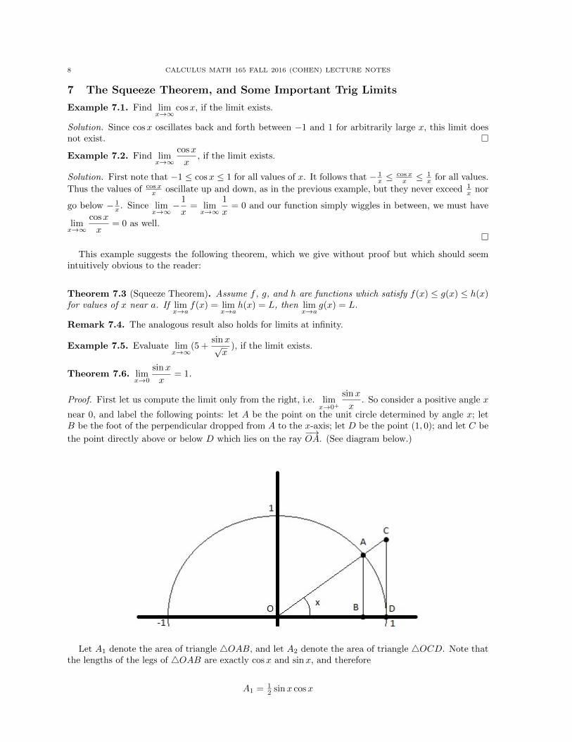
Proof. First let us compute the limit only from the right, i.e. limx→0+

sinx

x. So consider a positive angle x

near 0, and label the following points: let A be the point on the unit circle determined by angle x; letB be the foot of the perpendicular dropped from A to the x-axis; let D be the point (1, 0); and let C be

the point directly above or below D which lies on the ray−→OA. (See diagram below.)

Let A1 denote the area of triangle 4OAB, and let A2 denote the area of triangle 4OCD. Note thatthe lengths of the legs of 4OAB are exactly cosx and sinx, and therefore

A1 = 12 sinx cosx


by the familiar area formula for triangles. On the other hand 4OCD has a leg OD of length 1, and aleg CD of length tanx. Therefore

A2 = 12 tanx = sin x

2 cos x .

Lastly, consider the sector (i.e. pie slice) of the unit disk determined by the points O, A, and B. LetX denote the area of this sector. Since the area of the unit circle is π, we have

X = x2π · π = x

2 .

Now observe that regardless of the choice of x, the inequality A1 ≤ X ≤ A2 holds. Written otherwise,

12 sinx cosx ≤ x

2 ≤sin x

2 cos x .

Dividing by sinx (for values of x near 0 but not equal to 0) and multiplying by 2, we get

cosx ≤ xsin x ≤

1cos x

and therefore

cosx ≤ sin xx ≤ 1

cos x .

Now taking the limit of the three expressions above as x → 0, we see limx→0+

cosx = limx→0+

1

cosx= 1,

and therefore limx→0+

sinx

x= 1 by the Squeeze Theorem.

To see that limx→0−

sinx

x= 1 as well, simply note that both sinx and x are odd functions of x, i.e. their

graphs have a 180◦ rotation symmetry about the origin in the plane. Written out symbolically, we are

simply observing thatsin(−x)

−x=− sinx

−x=

sinx

x, and therefore the limits at 0 from the left and the

right must be the same. �

Corollary 7.7. limx→0

1− cosx

x= 0.

Proof. For x near 0, observe that

limx→0

1− cosx

x= limx→0

1− cosx

x· 1 + cosx

1 + cosx

= limx→0

1− cos2 x

x(1 + cosx)

= limx→0

sin2 x

x(1 + cosx)

= limx→0

(sinx

x

)(sinx

1 + cosx

)= 1 · 0

2= 0.

�



tanx

x, if it exists.


sin 6x

x, if it exists.


sin 7x

sin 4x, if it exists.


secx− 1

x, if it exists.

8 Differentiation

Definition 8.1. Let f(x) be any function, and a be any real number. The average rate of changeof f from x = a to x = b is given by:

f(b)− f(a)

b− a.

This is also the slope of the secant line connecting the points (a, f(a)) and (b, f(b)).

Example 8.2. Let f(x) = x2 + 4x. Find the average rate of change of f from x = 1 to x = 5.

Example 8.3. A ball is launched into the air, and its height in feet after t seconds is given by f(t) =−16t2 + 96t.

(1) Find the average velocity of the ball from t = 1 second to t = 4 seconds.(2) Find the average velocity of the ball from t = 1 second to t = 1 + h seconds, where h is any

small positive interval of time.

Definition 8.4. Let f be a function and a a real number. The difference quotient of f at a is theexpression

f(a+ h)− f(a)

h,

which computes the average rate of change of f from x = a to x = a+ h.

The instantaneous rate of change of f at x = a, or the slope of the tangent line to the graphof f at x = a, is given by:

limh→0

f(a+ h)− f(a)

h

Example 8.5. Let f(x) = x2 + 4x.

(1) Find the instantaneous rate of change (IROC) of f at x = 1.

(2) Find the equation of the line tangent to the graph of f at x = 1.

Solution. We compute the IROC of f at x = 1 below:

limh→0

f(1 + h)− f(1)

h= limh→0

[(1 + h)2 + 4(1 + h)]− [12 + 4(1)]

h

= limh→0

1 + 2h+ h2 + 4 + 4h− 1− 4

h

= limh→0

h2 + 6h

h= limh→0

(h+ 6)

= 6.


So the slope of the tangent line to the graph of f at x = 1 is 6. To find the equation of this line,we need only note that the line must meet the graph at the point (1, f(1)) = (1,−5), and apply thepoint-slope formula:

y − y1 = m(x− x1)y − (−5) = 6(x− 1)

y = 6x− 11

�

Definition 8.6. The derivative of f is the function

f ′(x) = limh→0

f(x+ h)− f(x)

h,

wherever this limit exists. If f ′(x) exists, we say that f is differentiable at the point x.

Remark 8.7. The main idea of the derivative is this: given a function f , we define a new function f ′,the derivative of f , which describes the behavior of the function f at each point x. Specifically, f ′ takesa real number x for input, and for output returns the slope of the tangent line to the graph of f at thepoint x, or equivalently, the instantaneous rate of change of f at x.

Example 8.8. Let f(x) = −16x2 + 96x. Find its derivative f ′(x). Compute f ′(1), f ′(0), f ′(3), f ′(5).Do the values make sense given the context of our physics example?

Solution. We compute the derivative by the definition below:

f ′(x) = limh→0

f(x+ h)− f(x)

h

= limh→0

[−16(x+ h)2 + 96(x+ h)]− [−16x2 + 96x]

h

= limh→0

−16x2 − 32xh− 16h2 + 96x+ 96h+ 16x2 − 96x

h

= limh→0

−32xh− 16h2 + 96h

h= limh→0−32x− 16h+ 96

= −32x− 16(0) + 96

= −32x+ 96.

So the derivative is f ′(x) = −32x+ 96.

Now we observe that f ′(1) = −32(1) + 96 = 64, which is the instantaneous velocity at x = 1 wecomputed earlier.

f ′(0) = −32(0) + 96 = 96, which is the velocity at which the ball is initially launched according toour original problem. (In other words, the instantaneous velocity at x = 0.

f ′(3) = −32(3) + 96 = 0. So the velocity at t = 3, the moment the ball tops out its arc and begins tofall back to the earth, is exactly 0, as expected.


f ′(5) = −32(5) + 96 = −64. So the velocity at t = 5, i.e. 2 seconds after the ball tops out its arc, is−64, i.e. the ball is falling toward the earth at 64 ft/s. Considering at t = 1 the ball was flying UP at64 ft/s, this should not be surprising! �

Remark 8.9 (Remark on Old-Fashioned Notations). The Greek letter ∆ is often used to representchange. So instead of h one may write ∆x, the “change in x.” Moreover instead of writing f(x+h)−f(x),one may regard this as the “change in y,” and write ∆y. So we have

f(x+ h)− f(x)

h=

∆y

∆x.

When computing the derivative, we wish to take take the limit as ∆x → 0. Now recall our earlierremarks about infinitesimals or “infinitely small distances”: this notion was used freely before and duringthe development of the calculus, before it was discarded for perceived lack of rigor, and replaced withthe modern notion of a limit. Leibniz’s work, however, significantly predates limits, and he thoughtin terms of infinitesimals. So in his notation, the “infinitely small” version of ∆x was denoted dx, aninfinitesimal distance, and he used dy to represent the corresponding infinitesimal change in y. Thus theLeibniz notation for the derivative is as follows:

lim∆x→0

∆y

∆x=dy

dx.

The Leibniz notation for the derivative has some advantages, but many drawbacks: in particular itconfusingly portrays the derivative function as some type of fraction (see Remark 12.5 for more on this).However, the Leibniz notation is extremely common and the student is sure to encounter it in futurecoursework. So we will use it in this course interchangeably with f ′(x).

Some other notations which also stand for the derivative of a function y = f(x) are the following: dfdx ,

ddxf(x), y′, y′(x).

Example 8.10. Let y = f(x) =√x.

(1) Find dydx .

(2) Find the equation of the line tangent to the graph of f at (4, 2).

Example 8.11. Let g(t) = 1t2 . Find g′(t).

Example 8.12. Graphical example: Sec 3.1 Example 5.

Example 8.13. Show that f(x) = |x| is not differentiable at x = 0.

Example 8.14. Show that f(x) = 3√x is not differentiable at x = 0.

Fact 8.15. If a function is differentiable at a point, then it must be continuous at that point. Theconverse, however, is not true: A function may be continuous at a point but not differentiable there.

A function is not differentiable at a point a if at least one of the following holds:

(1) f is not continuous at a.(2) f has a corner at a. (Example: f(x) = |x|.)(3) f has a vertical tangent at a. (Example: f(x) = x

13 .)

9 Rules of Differentiation

Remark 9.1. Many of our derivative calculations in the previous section were long, tedious, and/or com-putationally difficult. We wish to develop shortcuts by which one may rapidly compute the derivativesof familiar functions. We’ll begin by computing a few the old-fashioned way.

Example 9.2. Let c be any real number, and let f(x) = c. Find f ′(x).


Solution. Since the graph of f is a horizontal line, every tangent line to the graph should have slope 0.Thus we conjecture that f ′(x) = 0. Computing below, we see that our chosen definition of the derivativeconfirms our intuition:

f ′(x) = limh→0

f(x+ h)− f(x)

h= limh→0

c− ch

= limh→0

0 = 0. �

Theorem 9.3 (Constant Rule). If c is a real number, then

ddx (c) = 0.

Example 9.4. Find the following:

(1) ddx (x)

(2) ddx (x2)

(3) ddx (x3)

Solution. Some basic computations will show that the three derivatives are 1, 2x, and 3x2, respectively.It is also easy to show that d

dx (x4) = 4x3, ddx (x5) = 5x4, etc., which leads us to the following rule. �

Theorem 9.5 (Power Rule). For any exponent n, we have

ddx (xn) = nxn−1.

Example 9.6. Evaluate the following derivatives:

(1) ddx (x9)

(2) ddx (x275)

(3) ddx (28)

(4) ddx

3√x

(5) ddx

1x5

Theorem 9.7 (Constant Multiple Rule). If f is differentiable at x and c is a constant, then

ddx [cf(x)] = cf ′(x).

Theorem 9.8 (Sum Rule). If f and g are differentiable at x, then

ddx [f(x) + g(x)] = f ′(x) + g′(x).

Remark 9.9. The two rules above say that taking derivatives “distributes over” sums, differences, andmultiples of functions.

Example 9.10. Find ddx (2x3 + 9x2 − 6x+ 4).

Example 9.11. Let f(x) = 2x3 − 15x2 + 24x.

(1) Find an equation of the line tangent to the graph of f at the point (2, 4).

(2) At what points on the graph of f is the tangent line horizontal?

(3) For what values of x does the tangent line have a slope of 6?


10 The Product Rule and Quotient Rule

Remark 10.1 (A Naive Product Rule?). The ”sum rule” above tells us that derivatives ”distribute overaddition”, i.e. d

dx (f(x) + g(x)) = f ′(x) + g′(x) for any two functions f and g. We may be tempted toderive a similar conclusion for multiplication, i.e. that the derivative of a product of two functions is theproduct of the two derivatives. Unfortunately this is not the case, as the following example illustrates.

Example 10.2. Let f(x) = x2 and g(x) = x3.

(1) Find f ′(x), g′(x), and f ′(x) · g′(x).

(2) Find ddx (f(x)g(x)).

(3) Does ddx (f(x)g(x)) = f ′(x)g′(x)?

Solution. By the power rule we have f ′(x) = 2x and g′(x) = 3x2, so f ′(x) · g′(x) = 6x3. On the otherhand, (fg)(x) = x2 · x3 = x5, and hence (fg)′(x) = 5x4. So clearly we have d

dx (f(x)g(x)) 6= f ′(x)g′(x).

This example shows that the very simple “obvious” product rule is false. However, we can obtain arule which is almost as simple and nice, which is stated in the next theorem. �

Theorem 10.3 (Product Rule for Derivatives). If f and g are differentiable at x, then

ddx [f(x)g(x)] = f ′(x)g(x) + f(x)g′(x).

Proof. To show the product rule, we simply compute the derivative ddx [f(x)g(x)] below. Note in our

second line, we use the trick of adding and subtracting f(x)g(x+h)h to the equation (which is the same as

adding 0).

d

dx[f(x)g(x)] = lim

h→0

f(x+ h)g(x+ h)− f(x)g(x)

h

= limh→0

f(x+ h)g(x+ h)− f(x)g(x+ h) + f(x)g(x+ h)− f(x)g(x)

h

= limh→0

[f(x+ h)g(x+ h)− f(x)g(x+ h)

h+f(x)g(x+ h)− f(x)g(x)

h

]= limx→0

[f(x+ h)− f(x)

h· g(x+ h) + f(x) · g(x+ h)− g(x)

h

]=

[limx→0

f(x+ h)− f(x)

h

]( limh→0

g(x+ h)) + ( limh→0

f(x))

[limh→0

g(x+ h)− g(x)

h

]= f ′(x)g(x) + f(x)g′(x).

�

Example 10.4. Use the product rule to find the following derivatives:

(1) ddx [x2 · x3]

(2) ddx [(x3 − 8)(x2 + 4)]

(3) ddx [(7x5 − 4x2 + 8x)(14x3 − 19)]

Remark 10.5. Our next objective is to provide a “quotient rule” for derivatives as well. To emphasizethe importance of the order of the terms in this rule, we will change our function names from f and gto N and D, for “numerator” and “denominator” respectively.

Theorem 10.6 (Quotient Rule for Derivatives). If N and D are differentiable at x and D(x) 6= 0, then


d

dx

[N(x)

D(x)

]=D(x)N ′(x)−N(x)D′(x)

[D(x)]2.

Proof. This rule should follow easily from the product rule, if we set things up the right way. Set

q(x) = N(x)D(x) . We wish to compute q′(x).

First note that N(x) = q(x)D(x), so the product rule tells us that

N ′(x) = q′(x)D(x) + q(x)D′(x)

In that case, solving for q′(x), we have q′(x) = N ′(x)−q(x)D′(x)D(x) . In order to simplify this fraction, we

multiply by D(x)D(x) , and observe that q(x)D(x) = N(x)

D(x)D(x) = N(x) below:

q′(x) =N ′(x)− q(x)D′(x)

D(x)· D(x)

D(x)

=D(x)N ′(x)− q(x)D(x)D′(x)

[D(x)]2

=D(x)N ′(x)−N(x)D′(x)

[D(x)]2

So our quotient rule holds. �

Example 10.7. Find and simplify the following derivatives.

(1) ddx [x

2+3x+4x2−1 ]

(2) ddx (2x−3)

Example 10.8. Find an equation of the line tangent to the graph of f(x) = x2+1x2−4 at the point (3, 2).

11 Derivatives of Trigonometric Functions

Example 11.1. Sketch a rough graph of the derivative of f(x) = sinx.

Solution. The graph of f(x) = sinx has horizontal tangent lines at x = π2 ,

3π2 ,

5π2 , ..., etc., so we know

that f ′(x) = 0 at each of these points.

At x = 0, the graph of f(x) = sinx has some positive slope m, which will recur every 2π units upand down the real line. At x = π the graph should have slope −m, which will also recur every 2π units.

In general the graph of f ′(x) should look like a continuous periodic curve which oscillates back andforth between some values −m and m. In particular, if m = 1, then the graph of f ′(x) should call tomind the graph of cosx! �

Theorem 11.2 (Derivatives of Sine and Cosine). The following derivative formulas hold:

ddx sinx = cosx

and

ddx cosx = − sinx.

Proof. First compute the derivative of sinx, using the limit formulas we proved in Theorem 7.6 andCorollary 7.7. We use a common trig identity in line 2.


d

dxsinx = lim

h→0

sin(x+ h)− sinx

h

= limh→0

sinx cosh+ cosx sinh− sinx

h

= limh→0

[sinx

(cosh− 1

h

)+ cosx

(sinh

h

)]= sinx · 0 + cosx · 1= cosx.

Next using a similar method, compute the derivative of cosx.

d

dxcosx = lim

h→0

cos(x+ h)− cosx

h

= limh→0

cosx cosh− sinx sinh− cosx

h

= limh→0

[cosx

(cosh− 1

h

)− sinx

(sinh

h

)]= cosx · 0− sinx · 1= − sinx.

�

Example 11.3. Calculate dydx for the following functions.

(1) y = x2 cosx

(2) y = sinx− x cosx

(3) y = 1+sin x1−sin x

Example 11.4. Calculate ddx tanx using the quotient rule.

Theorem 11.5 (Derivative of Tangent and Cotangent). We have

ddx tanx = sec2 x

and

ddx cotx = − csc2 x.

Theorem 11.6 (Derivatives of Secant and Cosecant). We have

ddx secx = secx tanx

and

ddx cscx = − cscx cotx.

Proof. Do this using the quotient rule on sec = 1cos x and csc = 1

sin x . �

Example 11.7. Let y = secx cscx, and compute y′.


12 The Chain Rule

Remark 12.1. Recall: If f(x) and g(x) are two functions, then the composition of f and g, denotedby (f ◦ g), is defined by the rule (f ◦ g)(x) = f(g(x)). For example, if f(x) = x90 and g(x) = 5x + 4,then (f ◦ g)(x) = (5x + 4)90 and (g ◦ f)(x) = 5x90 + 4. We wish to be able to take derivatives ofsuch compositions of functions, so we need a new rule, which we give below. This rule is often easierunderstood through practice than by staring at the formula.

Theorem 12.2 (Chain Rule for Derivatives). Let f and g be differentiable functions. Then f ◦ g isdifferentiable and

(f ◦ g)′(x) = f ′(g(x)) · g′(x).

Example 12.3. Let f(x) = x90 and g(x) = 5x + 4. Find the derivative of (f ◦ g)(x) = f(g(x)) =(5x+ 4)90.

Solution. We already know f ′(x) = 90x89 and g′(x) = 5. The chain rule says to multiply the twoderivatives, but evaluate f ′(x) at the point g(x) as follows:

(f ◦ g)′(x) = f ′(g(x)) · g′(x) = 90(5x+ 4)89 · 5 = 450(5x+ 4)89.

�

Example 12.4. Find derivatives of the following functions.

(1) y = (7x3 − 5x)8

(2) y = (5x2 + 15)−2

(3) y = sin3 x

(4) y = sinx3

Remark 12.5. Now we wish to note that there is another way to view the chain rule, as a “substitution”rule. For example, consider the function y = (5x + 4)90, and suppose we wish to find the derivative

y′. Set u = 5x+4, so y = u90. Then dydu = 90u89 and du

dx = 5. In this case the chain rule says the following:

dydx = dy

du ·dudx

So we have y′ = dydx = [90u89] · [5] = 450u89 = 450(5x+ 4)89.

We should caution the student. Writing the chain rule in the above manner is simple and makes itvery easy to remember, as it jibes with our intuition of “cancelling out” terms in products of fractions.However, this intuition is misleading—derivatives are not fractions, and the fact that the functions dy

dx ,dydu , dudx are often written in this manner is an artifact of the obsolete notion of infinitesimals. (See Remark8.9.)

Example 12.6. Find ddx [√

5x2 + 1].

Example 12.7. Find ddt [(

5t2

3t2+2

)3

].

Example 12.8. Let y = sin(cosx2). Find y′.

Proof of the Chain Rule. The naive idea of the proof is as follows: We want to compute the derivativeof f ◦ g by rewriting the difference quotient as below.


(f ◦ g)′(x) = limh→0

f(g(x+ h))− f(g(x))

h

= limh→0

(f(g(x+ h))− f(g(x))

g(x+ h)− g(x)· g(x+ h)− g(x)

h

).

Naively, the expression on the left should go to f ′(g(x)) and the expression on the right should goto g′(x), as h → 0. However the problem with the above is that g(x + h) could be equal to g(x) forsmall values of h (for instance this is true if g(x) is a constant function). So the expression above is notnecessarily well-defined. We need to introduce a new function to fix this gap.

To repair the argument, let us treat x as a constant, and piecewise define a new function Q in avariable u:

Q(u) =

f(u)− f(g(x))

u− g(x): u 6= g(x);

f ′(g(x)) : u = g(x).

Thus Q(u) makes sense for any value of u. Observe also that limu→g(x)

Q(u) = Q(g(x)), since f is a

differentiable function at g(x). Therefore Q is continuous. Moreover, by our definition of Q, the followingequality holds for all h 6= 0:

f(g(x+ h))− f(g(x))

h= Q(g(x+ h)) · g(x+ h)− g(x)

h.

The above equality is clear when g(x+h) 6= g(x), just by plugging u = g(x+h) into Q. On the otherhand if g(x+ h) = g(x), then the equality holds because both sides are 0. So we have shown that

(f ◦ g)′(x) = limh→0

(Q(g(x+ h)) · g(x+ h)− g(x)

h

).

So computing (f ◦ g)′(x) amounts to computing the limit of the product above. Both limits in theproduct converge separately—we have lim

h→0Q(g(x + h)) = Q(g(x)) = f ′(g(x)) by the continuity of Q,

and limh→0

g(x+ h)− g(x)

h= g′(x) by the differentiability of g. Therefore (f ◦ g)′(x) = f ′(g(x))g′(x) as

claimed. �

13 Exponentials and Logarithms

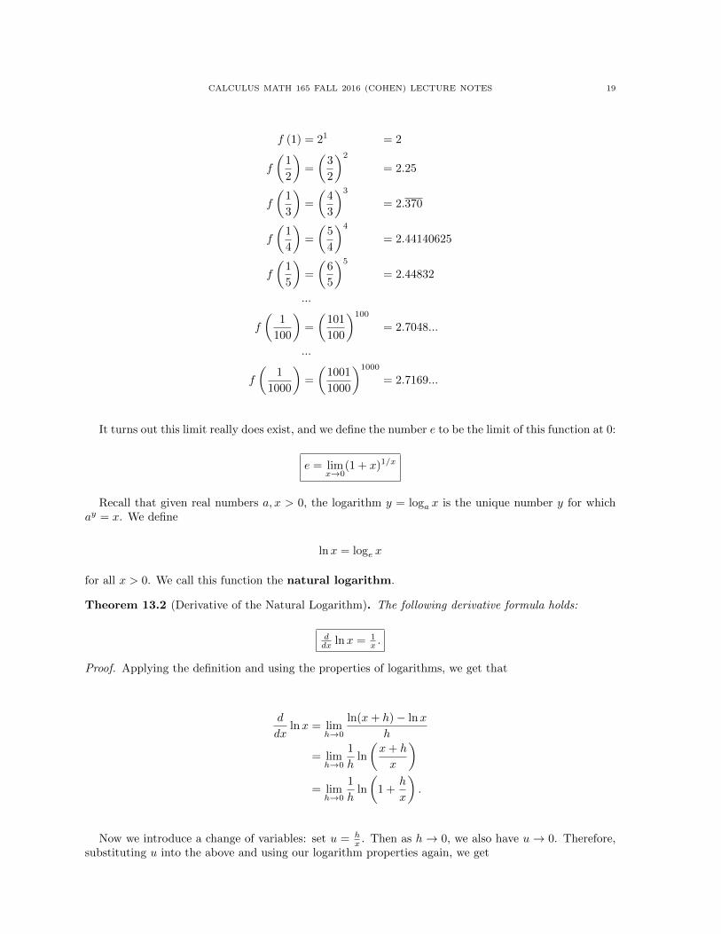
Definition 13.1 (Definition of e). Consider the function f(x) = (1 + x)1/x, defined for x > −1, x 6= 0.Examination of this function reveals a few properties: we see that f(0) is undefined, lim

x→−1f(x) = ∞,

and limx→∞

f(x) = 1. Via numerical approximation, we can see that f(x) appears to have a limit as x→ 0,

and this limit is somewhere between 2.5 and 3. For instance:


f (1) = 21 = 2

f

(1

2

)=

(3

2

)2

= 2.25

f

(1

3

)=

(4

3

)3

= 2.370

f

(1

4

)=

(5

4

)4

= 2.44140625

f

(1

5

)=

(6

5

)5

= 2.44832

...

f

(1

100

)=

(101

100

)100

= 2.7048...

...

f

(1

1000

)=

(1001

1000

)1000

= 2.7169...

It turns out this limit really does exist, and we define the number e to be the limit of this function at 0:

e = limx→0

(1 + x)1/x

Recall that given real numbers a, x > 0, the logarithm y = loga x is the unique number y for whichay = x. We define

lnx = loge x

for all x > 0. We call this function the natural logarithm.

Theorem 13.2 (Derivative of the Natural Logarithm). The following derivative formula holds:

ddx lnx = 1

x .

Proof. Applying the definition and using the properties of logarithms, we get that

d

dxlnx = lim

h→0

ln(x+ h)− lnx

h

= limh→0

1

hln

(x+ h

x

)= limh→0

1

hln

(1 +

h

x

).

Now we introduce a change of variables: set u = hx . Then as h→ 0, we also have u→ 0. Therefore,

substituting u into the above and using our logarithm properties again, we get


d

dxlnx = lim

u→0

1

xuln(1 + u)

= limu→0

1

xln(1 + u)1/u

=1

x· ln(

limu→0

(1 + u)1/u)

=1

x· ln e

=1

x.

Note that in line 3 of the equality above, we used the fact that lnx is a continuous function to pullthe limit inside. This completes the proof. �

Example 13.3. Compute ddx ln(x3 + 10x).

Corollary 13.4 (Derivative of the Exponential Function). The following derivative formula holds:

ddxe

x = ex.

Proof. Let f(x) = ex and let g(x) = lnx. Note that

g(f(x)) = x.

Therefore, taking the derivative of both sides and using the chain rule, we get

g′(f(x)) · f ′(x) = 1.

But g′(f(x)) = 1ex . So the line above says 1

ex · f′(x) = 1. Therefore f ′(x) = ex. �

Example 13.5. Find ddxe

7x.

Example 13.6. Find ddx5x.

Theorem 13.7 (Derivatives of General Exponential Functions). Let b > 0. Then

ddxb

x = (ln b)bx.

Proof. Compute using the chain rule that

d

dxbx =

d

dx(eln b)x

=d

dxe(ln b)x

= (ln b)e(ln b)x

= (ln b)bx.

�

Example 13.8. Find f ′(x) for the following.

(1) f(x) = 43x

(2) f(x) = 5x2


(3) f(x) = 10x lnx

Theorem 13.9 (Derivatives of General Logarithms). Let b > 0. Then

ddx logb x = 1

(ln b)x .

Proof. This is immediate from the fact that logb x = ln xln b . �

Example 13.10. Compute y′ for the following.

(1) y = xx

(2) y = xsin x

Solution. There are two good methods for solving these two (similar) derivative problems. We will doone method for each.

For y = xx, simply rewrite as y = (eln x)x = ex ln x. Then the derivative using the chain rule and theproduct rule is

y′ = (lnx+ 1)ex ln x = (lnx+ 1)xx.

For the second problem y = xsin x, let us introduce the logarithm on both sides and write

ln y = lnxsin x = sinx lnx.

Next take the derivative of both sides with respect to x. Since y is a function of x, the chain ruleimplies that d

dx ln y = 1y · y

′. Therefore

1y · y

′ = cosx lnx+ sinx · 1x .

Multiplying both sides above by y = xsin x yields

y′ =(cosx lnx+ sin x

x

)xsin x.

�

14 Maxima and Minima

Definition 14.1. Let f be defined on an interval containing c. Then f has an absolute maximumvalue on I at c is f(c) ≥ f(x) for every x ∈ I. Similarly, f has an absolute minimum value on I at cis f(c) ≤ f(x) for every x in I.

Example 14.2. Graphical examples: f(x) = x2 on: (−∞,∞), [0, 2], (0, 2], and (0, 2).

Remark 14.3. From the above examples we see that determining absolute maxima and minima dependson not only the function f but also the choice of interval I. However, we can guarantee their existenceby requiring two things: first, that f be continuous, and second, that I contain its endpoints.

Theorem 14.4 (Extreme Value Theorem). A function that is continuous on a closed interval [a, b] hasan absolute maximum value and an absolute minimum value on that interval.

Definition 14.5. Let f be defined at c. If there exists some open interval I containing c, such that fis defined on I, and f(c) ≥ f(x) for all x in I, then f(c) is a local maximum of f . If f(c) ≤ f(x) forall x in I, then f(c) is a local minimum of f .

We also refer to local maxima (and minima) as relative maxima (and relative minima). If f(c) is amaximum (or minimum) then we say f has a maximum at x = c (or a minimum at x = c.


Remark 14.6. Now, suppose that f is some polynomial function. Polynomials are continuous anddifferentiable at every point, so its graph should look like some smooth curve, perhaps winding up anddown, and eventually going to either∞ or −∞ in either the left or right direction. How can we computeat which points f has local maxima or local minima?

It should be clear by now that for a smooth curve (like that of a polynomial) the only places x wheref can “top out” or “bottom out” (i.e. have a local maximum or minimum) are points where the tangentline to the graph is horizontal, i.e. where f ′(x) = 0. In fact, this applies to any differentiable function:If c is some point where f ′(c) exists, and such that f has a local maximum or local minimum at x = c,then f ′(c) = 0.

On the other hand, we know that it is possible to have a local maximum or minimum at points whereno derivative exists. For example, if f(x) = |x|, then f has a corner point at x = 0, so f ′(0) does notexist, but f certainly has a minimum at x = 0. It is also possible to have local maxima/minima atpoints of discontinuity, and if f is discontinuous at a point then it has no derivative there. These cases,however, account for all the possibilities: if f has a local maximum or minimum at x = c, then eitherf ′(c) = 0 or f is not differentiable at c. This leads us to the following definition.

Definition 14.7. Suppose f is defined at the point c. We say c is a critical point of f if eitherf ′(c) = 0 or if f ′(c) does not exist.

Fact 14.8. If f has a local maximum/minimum at x = c, then c must be a critical point of f .

Remark 14.9. On the other hand, if c is a critical point, then f does not necessarily have a localmaximum or minimum at c. For example, consider f(x) = x3 or f(x) = 3

√x at x = 0.

Example 14.10. Find the critical points of f(x) = xx2+1 .

Example 14.11. Find the absolute maximum and minimum values of the following:

(1) f(x) = x4 − 2x3 on the interval [−2, 2]

(2) g(x) = x23 (2− x) on the interval [−1, 2]

Solution. We will solve part (a) and leave part (b) to the student. By the Extreme Value Theorem weknow that an absolute maximum and minimum value for f on [−2, 2] are guaranteed to exist. Suchvalues can only occur at either the critical points of f , or at the endpoints of the interval [−2, 2]. So allwe need to do is find the critical values of f , and determine at which of the points f takes its highestand lowest values.

We start by finding the derivative f ′(x) = 4x3−6x2. Since f ′ is a polynomial, it is defined everywhere,so there will be no critical values x for which f ′(x) does not exist. Then we need only find all points xwhere f ′(x) = 0:

4x3 − 6x2 = 0

2x2(2x− 3) = 0

So either 2x2 = 0 or 2x− 3 = 0; this gives us two solutions, x = 0 and x = 32 . To finish the problem

we test f at the two critical values x = 0 and x = 32 , and also at the endpoints x = −2 and x = 2.

f(0) = 0f( 3

2 ) = − 2716

f(−2) = 32f(2) = 0


So f obtains an absolute maximum of 32 at x = −2 and an absolute minimum of − 2716 at x = 3

2 . �

15 Increasing and Decreasing Functions

Definition 15.1. Suppose f is a function defined on an interval I. We say f is increasing if, wheneverx1 and x2 are in I and x1 < x2, then f(x1) < f(x2). We say f is decreasing if whenever x1 and x2 arein I and x1 < x2, then f(x1) > f(x2).

Fact 15.2. If f is differentiable on I and f ′(x) > 0 for all x in I, then f ’s tangent lines all have apositive slope, and hence f is increasing on I. Likewise if f ′(x) < 0 for all x in I, then f is decreasingon I.

Example 15.3. Sketch a function f which is continuous on (−∞,∞) and satisfies the following:

(1) f ′ > 0 on (−∞, 0), (4, 6), and (6,∞)

(2) f ′ < 0 on (0, 4)

(3) f ′(0) is undefined

(4) f ′(4) = f ′(6) = 0

Example 15.4. Find the intervals on which f(x) = 2x3 + 3x2 + 1 is increasing and decreasing.

Example 15.5. Find all local maxima and minima of f(x) = 2x3 + 3x2 + 1.

Theorem 15.6 (First Derivative Test). Suppose f is continuous on an interval I that contains a pointx, and f is differentiable on I (except possibly at the point c).

(1) If f ′ changes sign from positive to negative as x increases through c, then f has a local maximumat c.

(2) If f ′ changes sign from negative to positive as x increases through c, then f has a local minimumat c.

(3) If f ′ does not change sign at c then f has no local extreme value at c.

Example 15.7. Let f(x) = 3x4 − 4x3 − 6x2 + 12x+ 1. Find all local extrema of f .

Example 15.8. Find all local extrema of f(x) = x23 (2− x).

Example 15.9. Find all absolute extrema of f(x) = 14x

4 − x3 + 32x

2 − 9x+ 2.

16 Concavity

Definition 16.1. Let f be a differentiable function, and assume its derivative f ′ is also differentiable.We denote by f ′′ the second derivative of f , defined by

f ′′(x) = ddxf′(x).

Similarly we may define the third derivative f ′′′, fourth derivative f ′′′′, etc., when they exist.For any positive integer n (especially n > 2) we denote by f (n) the n-th derivative of f , if it exists.

Remark 16.2. We wish to apply the notion of a second derivative to our optimization problems. As amotivating example, consider the graph of f(x) = x3. For values of x > 0, the curve of the graph bendsupward. In other words, as we move from left to right, the tangent lines get steeper. In other words, thefirst derivative f ′ is increasing. Since f ′ is differentiable, we know that the second derivative f ′′ mustsatisfy f ′′(x) > 0 for all x > 0. We refer to this portion of the graph as concave up.


On the other hand, for all values of x < 0, the curve of the graph bends downward, i.e. the graphis concave down. As we move left to right on the graph, the tangent lines become less steep, i.e. thefirst derivative f ′ is decreasing, i.e. the second derivative f ′′ satisfies f ′′(x) < 0 for all x < 0.

Definition 16.3. Let f be differentiable on an open interval I. If f ′ is increasing on I then f is concaveup on I. If f ′ is decreasing on I that f is concave down on I. If f is continuous at c and f changesconcavity at c (from up to down, or vice versa), then f has an inflection point at c.

Fact 16.4. If a graph is concave up at a given point x, then the graph near the point lies above thetangent line at x. Conversely if the graph is concave down at x, then the graph near the point lies belowthe tangent line at x.

Example 16.5. Graphical example which shows no explicit relationship between the concavity of afunction and whether it is increasing or decreasing. (A function can be increasing and concave down, ordecreasing and concave up, or any other combination of these properties.)

Example 16.6. Let f(x) = 3x4 − 4x3 − 6x2 + 12x+ 1. Identify the intervals on which f is concave upor concave down, and find any inflection points.

Theorem 16.7 (Second Derivative Test). Suppose that f ′′ is continuous on an open interval containingc with f ′(c) = 0.

(1) If f ′′(c) > 0 then f has a local maximum at c.

(2) If f ′′(c) < 0 then f has a local minimum at c.

(3) If f ′′(c) = 0, then the test is inconclusive.

Example 16.8. Use the Second Derivative Test to find all local extrema of f(x) = 2x3 − 3x2 + 12.

17 Some Optimization Problems

Example 17.1. Consider all pairs of positive numbers whose product is 10000. Is there a pair withminimal sum? Is there a pair with maximal sum? If so, identify the pairs.

Solution. Notice that there can be no maximal such pair, for if x is ANY positive real number, then

x · 10000

x= 10000, and x+

10000

xis bigger than x. Since we can choose x as large as we want, we can

get sums as large as we want.

On the other hand, we can use calculus to prove that there is a minimal such pair. The first step isto define an sum function, which, intuitively speaking, should take a pair of numbers which multiply to10000 as input and spit out the sum of the pair as output. Then all we need to do is find the absoluteminimum of this function using the techniques we have learned.

This function is easy to define but we need to make one change in order to use our techniques. Let xand y be any two numbers whose product is 10000; then their sum is given by:

S(x, y) = x+ y

Our only problem with the above sum function is that it takes two variables for input, and we wouldlike it to be a single-variable function. Note, now, that x and y are not independent pieces of information-that is, if x is any particular positive number, then there is exactly one y for which xy = 10000! In fact,

we have y =10000

xfor any chosen x. We can now substitute this equality into our sum function to get

a function in one variable:


S(x) = x+10000

x= x+ 10000x−1

Now we maximize S(x). We have S′(x) = 1− 10000x−2. This derivative is 0 if x = 100 or x = −100,and is undefined at x = 0, so we have three critical points. But the problem asks us about positivenumbers, so we need only consider the single critical point x = 100.

Since S′′(x) = 20000x−3, applying the second derivative test at x = 100 yields S′′(100) =1

50> 0. So

S is concave up at x = 100 and hence S indeed has a minimum value at x = 100.

If x = 100 then y = 100 and S = 100 + 100 = 200 is the minimum possible sum. �

Remark 17.2 (Strategy for Optimization Word Problems). In the previous example, we (1) built ageneral “sum” function S = x + y; (2) reduced S to to a function of one variable by observing thatxy = 10000 and subsituting for y; and (3) minimized S with our calculus techniques. This process is atypical example of the following general strategy:

(1) Identify what you are being asked to maximize or minimize, and build a function which expressesthis value in terms of any possible inputs.

(2) Use any constraints given in the problem to reduce your function to just one variable input.(3) Optimize your function using calculus.

Example 17.3. Let P be any fixed positive number, and consider all rectangles that have perimeterP . Is there such a rectangle with maximal area? Is there one with minimal area? If so, identify therectangles.

Example 17.4. A rancher wishes to build a rectangular corral using 400 ft of fencing. One wall of thecorral will lie alongside a barn, so the rancher doesn’t have to use any fencing on one side. The corralwill be split into three congruent rectangular sections, each with one wall alongside the barn. Whichdimensions should the rancher choose for his corral in order to maximize its area?

18 Implicit Differentiation

Remark 18.1. Up to this point we have restricted our attention to functions which are defined explicitly,e.g. we say y = f(x) where f is some function, and we compute the derivative y′. Now we wish toconsider the concept of differentiation where the relationship between variables is defined implicitly. Forexample, the set of all solutions to the equation x2 + y2 = 1 is all the points on the unit circle. In thiscase, y is not a function of x (as the vertical line test fails) and x is not a function of y, but it still makessense to consider tangent lines to the graph of the unit circle. The chain rule now gives us the tool weneed to find a reasonable derivative function y′.

Example 18.2. Consider the unit circle x2 + y2 = 1. Find the slope of the tangent line to the unit

circle at ( 12 ,√

32 ) and (1

2 ,−√

32 ).

Solution. We will take the derivative of both sides of the equation x2 + y2 = 1. The crucial idea we willuse is that although y is not globally a function of x, if we restrict our attention to a sufficiently smallregion around a point where the tangent line to the circle is non-vertical, then locally y can be regardedas a function of x.

Treating y as a function of x, by the chain rule, the derivative of y2 (with respect to x is given byddxy

2 = ( ddyy2) · dydx = 2y · dydx . We now compute y′ below:


d

dx[x2 + y2] =

d

dx(1)

d

dx(x2) +

d

dx(y2) = 0

2x+

(d

dyy2

)(dy

dx

)= 0

2x+ 2y · dydx

= 0

y′ =dy

dx= −x

y

Notice that y′ depends on both y and x! This should not be surprising, as the x-coordinate aloneis not sufficient to pick out a point on the unit circle. We can now compute the appropriate slopes:

y′( 12 ,√

32 ) = − 1√

3and y′( 1

2 ,−√

32 ) = 1√

3. �

Example 18.3. Find an equation of the line tangent to the curve x2 + xy − y3 = 7 at (3, 2).

Example 18.4. Find the slope of the tangent line at the point (1, 1) on the graph of ex−y = 2x2 − y2.

Example 18.5. Find y′′ if y is defined implicitly by the rule x2 + 4y2 = 7.

Theorem 18.6 (Derivatives of Arcsine and Arccosine). Let arcsinx denote the inverse function of sinxwith domain [−1, 1] and range [−π2 ,

π2 ] (i.e. the function for which sin arcsinx = x for all x in [−1, 1]

and arcsin sinx = x for all x in [−π2 ,π2 ]. Similarly, let arccosx denote the inverse function of cosx with

domain [−1, 1] and range [0, π]. For all x in the domain of either function, we have

ddx arcsinx = 1√

1−x2

andddx arccosx = − 1√

1−x2.

Proof. For the function y = arcsinx, write x = sin y and use implicit differentiation to take the derivativeof both sides of the equation with respect to x.

sin y = x

cos y ·(dy

dx

)= 1

dy

dx=

1

cos y.

Written otherwise, we have computed that y′ = 1cos arcsin x . To finish the computation, consider a right

triangle with angle y = arcsinx, where x is a member of the interval [−π2 ,π2 ] as specified in the definition

of arcsinx. The ratio of opposite/hypotenuse in this triangle is x = x/1. If we label the opposite x

and the hypotenuse 1, then by the Pythagorean theorem, the adjacent has length√

1− x2. Thereforecos y = 1√

1−x2and we get

dydx = 1√

1−x2

as claimed in the theorem. The computation for arccosx is very similar and we omit it. �

Example 18.7. Calculate f ′( 12 ), where f(x) = arcsin(x2).


Theorem 18.8 (Derivatives of Other Inverse Trigonometric Functions). Labeling the inverse trigono-metric functions in the usual way, we have

ddx arctanx = 1

1+x2

ddxarccotx = − 1

1+x2

ddxarcsecx = 1

|x|√x2−1

ddxarccscx = − 1

|x|√x2−1

19 Related Rates

Example 19.1. An oil rig springs a leak in calm seas and the oil spreads in a circular patch aroundthe rig. If the radius of the oil patch increases at a rate of 30 m/hr, how fast is the area of the patchincreasing when the patch has a radius of 100 m?

Solution. Recall that the relationship between the radius r and the area A of a circle is given by theformula A = πr2. Now let t represent the time variable; in this case, both A and r will increase as afunction of t (since the oil spill is spreading as time passes). We can write A = A(t) and r = r(t) toemphasize that they are both functions of time.

In this case r′(t) will be the rate of change of the radius of the spill with respect to time, and A′(t)will be the rate of change of the area with respect to time. We will now use implicit differentiation toreveal the relationship between the two derivatives:

A′(t) =d

dt[π(r(t))2]

= πd

dt(r(t))2

= π · 2(r(t))r′(t)

= 2πr(t)r′(t)

Now we substitute the values specified in the word problem, i.e. we take r(t) = 100 and r′(t) = 30.Then the rate of change of the area is A′(t) = 2π(100)(30) = 6000π. (This should be interpreted assquare meters per hour.) �

Example 19.2. Two airplanes approach an airport, one flying due west at 120 mi/hr and the otherflying due north at 150 mi/hr. Assuming they fly at the same constant elevation, how fast is the distancebetween the planes changing when the westbound plane is 180 mi from the airport and the northboundplane is 225 mi from the airport?

Example 19.3. An observer stands 200 m from the launch site of a hot air balloon. The balloon risesvertically at a constant rate of 4 m/s. How fast is the angle of elevation of the baloon increasing 30 safter the launch?

20 L’Hospital’s Rule

Theorem 20.1 (L’Hospital’s Rule). Suppose f and g are functions differentiable at x = a, and limx→a

f(x)

g(x)is of indeterminate form 0

0 or ∞∞ , i.e. either


limx→a

f(x) = limx→a

g(x) = 0,

or else

limx→a

f(x) = ±∞ and limx→a g(x) = ±∞.

Then

limx→af(x)g(x) = limx→a

f ′(x)g′(x)

provided the limit on the right-hand side exists (or is equal to ±∞).

Example 20.2. Use L’Hospital’s rule to verify the limits in the examples above.

Example 20.3. Evaluate the following limits:

(1) limx→1

x3 + x2 − 2x

x− 1

(2) limx→0

√9 + 3x− 3

x

(3) limx→2

x3 − 3x2 + 4

x4 − 4x3 + 7x2 − 12x+ 12

Example 20.4 (L’Hospital’s Rule is Inapplicable). Evaluate limx→1

x2 + cosπx

x2 − 4x+ 2.

Example 20.5. Evaluate limx→2

4− x2

sinπx.

Example 20.6. Evaluate limx→0

ex − x− 1

cosx− 1.

Example 20.7 (Indeterminate Form ∞−∞). Evaluate limx→0

(1

sinx− 1

x

).

Example 20.8 (Indeterminate Form ∞ · 0). Evaluate limx→∞

x2 sin(1

4x2).

Example 20.9 (Indeterminate Form 00). Evaluate limx→0+

xx.

Example 20.10 (Indeterminate Form 1∞). Evaluate limx→0

(1 + 4x)12x .

Definition 20.11. Let f and g be two functions which satisfy limx→∞

f(x) = limx→∞

g(x) =∞. We say that

f(x) grows faster than g(x) if

limx→∞

f(x)

g(x)=∞, or equivalently, lim

x→∞

g(x)

f(x)= 0.

We denote this relationship by writing g(x) << f(x).

Example 20.12. Which function grows faster, f(x) = x2 or g(x) = x lnx?

Example 20.13. Rank the following functions in order of growth rate:

(1)√x;

(2) (lnx)3;(3) ex; and(4) 1.0001x.


21 Rolle’s Theorem and the Mean Value Theorem

Theorem 21.1 (Rolle’s Theorem). Let f be continuous on a closed interval [a, b] and differentiable onthe open interval (a, b). Suppose f(a) = f(b). Then there is at least one point c in (a, b) such thatf ′(c) = 0.

Proof. Since f is continuous on [a, b], by the Extreme Value Theorem 14.4 f must obtain some absolutemaximum and absolute minimum value on [a, b]. Either f obtains both its maximum and minimum atthe endpoints of the interval (x = a and x = b), or else f obtains one of its extreme inside the openinterval (a, b). We will consider both cases.

Case 1: Suppose f has its local maximum and local minimum at either x = a or x = b. Butf(a) = f(b) by our hypothesis, so if f doesn’t go above or below these values, then f must in fact be aconstant function. So f(x) = K for some number K. Then f ′(x) = 0 for every point in (a, b).

Case 2: Suppose instead that f obtains a local extreme value at some point x = c in the middleinterval (a, b). Then f must have a critical point at c, i.e. f ′(c) = 0 or f ′(c) does not exist. But weassumed f is differentiable on (a, b), so f ′(c) DOES exist; therefore f ′(c) = 0.

In either case 1 or case 2 we have produced a point c in (a, b) with f ′(c) = 0, so the theorem isproved. �

We will now use Rolle’s Theorem to prove the Mean Value Theorem, a stronger result.

Theorem 21.2 (Mean Value Theorem). Let f be continuous on a closed interval [a, b] and differentiableon the open interval (a, b). Then there is at least one point c in (a, b) such that

f(b)− f(a)

b− a= f ′(c).

Restated, there is some point c in (a, b) where the slope of the tangent line at (c, f(c)) is the same asthe slope of the secant line connecting the points (a, f(a)) and (b, f(b)).

Proof. Let `(x) be the linear function whose graph is the line passing through (a, f(a)) and (b, f(b)).Define a new function g(x) by the rule g(x) = f(x) − `(x), for all x in [a, b]. The function g(x) is justa difference of continuous differentiable functions and hence it is continuous and differentiable as well.Notice that g(a) = f(a) = `(a) = f(b) − f(b) = 0 and g(b) = f(b) − `(b) = f(b) − f(b) = 0, since`(a) = f(a) and `(b) = f(b). Hence g(a) = g(b), and therefore the function g(x) meets the conditionsrequired in Rolle’s Theorem 21.1.

In that case, Rolle’s Theorem implies that for some c in (a, b), we must have g′(c) = 0. But then wehave g′(c) = f ′(c) − `′(c) = 0 and hence f ′(c) = `′(c). Since the graph of `(x) is just the line between

(a, f(a)) and (b, f(b)), we have `′(c) = f(b)−f(a)b−a ; so f ′(c) = f(b)−f(a)

b−a as required. �

Remark 21.3. Notice that the Mean Value Theorem obvious implies Rolle’s Theorem, since if f(a) =

f(b), then the slope f(b)−f(a)b−a is just 0, so there is some point c in (a, b) with f ′(c) = 0. However, since

we can use Rolle’s Theorem to prove the Mean Value Theorem, the two really have basically the samecontent; the Mean Value Theorem is just Rolle’s Theorem adjusted for alteration by some linear function`(x).

Why do we care about the Mean Value Theorem? Let’s investigate some immediate consequences.

First suppose f(x) is any continuous function for which f ′(x) = 0 at every point x. Then givenany two numbers a and b (with a < b), choosing any point c in (a, b) yields f ′(c) = 0. Hence for the

Mean Value Theorem to be true, we must have that the slope f(b)−f(a)b−a is just 0. This only happens

if f(b) − f(a) = 0, i.e. if f(a) = f(b). Since this is true for ANY a and b, f must be a CONSTANTfunction, i.e. f(x) = C for some number C.


Then what can we say about two functions which have the same derivative? Suppose f and g arecontinuous functions such that f ′(x) = g′(x) for every x. Then f ′(x)− g′(x) = 0 everywhere, and hencethe above paragraph applies that f(x) − g(x) = C for some constant C. Then f(x) = g(x) + C, i.e. fand g differ only by some constant.

This is relevant because we wish to define the notion of an antiderivative in the near future, i.e. wewish to define a process which is the inverse of differentiation. Now we know that if f is some continuousfunction, then any two antiderivatives of f must be the same, except for some constant term. This factis crucial to understanding antidifferentiation.

22 Antiderivatives

Definition 22.1. A function F is an antiderivative of f on an interval I provided F ′(x) = f(x) forall x in I.

Theorem 22.2. Let F be any antiderivative of f . Then all antiderivatives of f have the form F + C,where C is some constant.

Proof. We proved this in our discussion of the Mean Value Theorem above. �

Example 22.3. Find all antiderivatives of the following functions:

(1) f(x) = 1

(2) f(x) = x

(3) f(x) = x2

(4) f(x) = x3

Fact 22.4 (Power Rule for Antiderivatives). Let p be any rational number (with p 6== −1). Then allantiderivatives of xp have the form

1p+1x

p+1 + C,

where C is some constant.

Example 22.5. Find all antiderivatives of f(x) = 3x5 + 2− 5x−32 .

Definition 22.6. To denote the operation “find all antiderivatives of f ,” we write the following:

∫f(x)dx

We refer to this string of symbols as the indefinite integral of f , and it refers to an infinite collectionof functions (all of which differ from one another by just a constant). We use this term indefinite integralinterchangeably with antiderivative.

We call the function f(x) the integrand. The term dx in the notation indicates that we are antidif-ferentiating with respect to the variable x.

Remark 22.7. This notation, like ddx and dy

dx , is also old-timey and wrapped up in the notion of“infinitesimals.” We will simply take the symbols at face value for now, and try to motivate theirmeaning later on when we start talking about definite integrals.

Example 22.8. Find∫

cos(3x)dx.

Fact 22.9 (Indefinite Integrals of Trigonometric Functions). The following all hold for any constanta 6= 0:


(1)∫

cos(ax)dx = 1a sin(ax) + C

(2)∫

sin(ax)dx = − 1a cos(ax) + C

(3)∫

sec2(ax)dx = 1a tan(ax) + C

(4)∫

csc2(ax)dx = − 1a cot(ax) + C

(5)∫

sec(ax) tan(ax)dx = 1a sec(ax) + C

(6)∫

csc(ax) cot(ax)dx = − 1a csc(ax) + C


(1)∫

sec2(7x)dx

(2)∫

cos(x2 )dx

Fact 22.11 (Indefinite Integrals of Exponentials and Logarithms). The following hold for any constantsa 6= 0, b > 1:

(1)∫ekxdx = 1

kekx + C

(2)∫bkxdx = 1

k ln bbkx + C

(3)∫

1xdx = ln |x|+ C


(1)∫

( 5x − 3x−10)dx

(2)∫

(3ex − 4)dx

(3)∫

(12e7−3x)dx

Example 22.13. Find the function y which satisfies y′ = 4x7 and y(0) = 4.

Example 22.14. Solve the equation dydx = sin(πx) subject to the condition y(2) = 2.

23 Approximating Areas Under Curves Using Riemann Sums

Example 23.1. Consider a car moving at a constant rate of 60 mi/hr. How far does the car move inexactly 3 hours? We know immediately that the answer is (60 mi/hr) · (3 hr) = 180 miles. How canwe visualize this solution geometrically? Consider the graph of the velocity equation v(t) = 60, i.e. thegraph of the horizontal line at height 60. The distance traveled after t seconds is always given by theequation 60 · t, which is exactly the area under the graph between t = 0 and t = 3. (Recall that thederivative of a distance function gives a velocity function, and in this case the area under the curveof a velocity function gives a distance function; this foreshadows the inverse relationship between thederivative and the integral!)

Now if a graph is given by a straight line, it is easy to compute the area under the curve by a simplegeometric formula; however we wish to compute the exact areas under graphs of more complicatedfunctions.

Example 23.2. Suppose the velocity in m/s of a moving object is given by the equation v(t) = t2, for0 ≤ t ≤ 8. Estimate the displacement of the object after 8 seconds.


Solution. One approach we may take is to divide the interval [0, 8] into, say, four equal subintervals andtry to estimate the displacement in each subinterval, i.e. make an estimate for every 2 seconds that passand then add them together. For instance, in the first two seconds the velocity of the object increasesfrom v(0) = 0 to v(2) = 4; we can perhaps get a decent approximation of the object’s velocity over thisinterval by taking v(1) = 1 m/s. Then we estimate that the object moves approximately (1 m/s) · (2s) = 2 m in the first 2 seconds.

Then we can make similar estimates for the remaining intervals: say the object moves about v(3) = 9m/s from t = 2 to t = 4; about v(5) = 25 m/s from t = 4 to t = 6; and about v(7) = 49 m/s from t = 6to t = 8. Then we may compute an estimate of the displacement of the object as follows:

v(1) · 2 + v(3) · 2 + v(5) · 2 + v(7) · 2 = (1 + 9 + 25 + 49) · 2 = 168 m.

Notice that we can visualize the product v(1) · 2 as the area of the rectangle with base [0, 2] andheight v(1) = 1. Likewise the next product v(3) · 2 corresponds to the area of the rectangle with base[2, 4] and height v(3); and so forth with the others. So what we are really computing is the sum of theareas of these four rectangles; geometrically, we are approximating the area under the curve of the graph.

What happens if we repeat this process by dividing the interval into, say, 8 subintervals instead of 4?What about 16, or 100, or 1000 subintervals? �

Definition 23.3. Suppose [a, b] is a closed interval. We may break up [a, b] into n distinct subintervals[x0, x1], [x1, x2],...,[xn−1, xn] of equal length ∆x = b−a

n with a = x0 and b = xn. The endpointsx0, x1, ..., xn are called grid points and they create a regular partition of [a, b]. In general, the k-thgrid point is xk = a+ k∆x, for k = 0, 1, ..., n.

Example 23.4. (1) Find a regular partition of [1, 9] into 4 subintervals.

(2) Find a regular partition of [5, 7] into 9 subintervals.

Definition 23.5. Suppose f is a function defined on a closed interval [a, b], and let x0, ..., xn give aregular partition of [a, b] into n subintervals. Let xk be any point in the k-th subinterval [xk−1, xk], foreach k = 1, 2, ..., n. Then the sum

f(x1)∆x+ f(x2)∆x+ ...+ f(xk)∆x

is called a Riemann sum for f on [a, b].

Furthermore, we call this sum a left Riemann sum if xk is always the left endpoint of [xk−1, xk]; aright Riemann sum of xk is always the right endpoint; and a midpoint Riemann sum of xk is alwaysthe midpoint.

Example 23.6. Find a regular partition for [0, 1] into 4 subintervals; then compute a left, right, andmidpoint Riemann sum for f(x) = x3 using this partition. How do the area estimates compare to theactual area under the curve?

Definition 23.7 (Sigma Notation for Sums). Now that we are working with Riemann sums of n terms,where n may be extremely large, it is in our interest to develop some new notation to describe when weare adding together a large finite number of terms.

Suppose we wish to represent the sum of the first 1000 perfect squares, i.e. 12 + 22 + 32 + ...+ 9992 +10002. We introduce the following string of symbols to represent this sum:∑1000

k=1 k2

The Greek letter∑

, i.e. the capital sigma, is an S for “Sum.” The “k = 1” below the sigma and the“1000” above the sigma tell us how many terms we wish to add together: in particular, we should startcounting terms from k = 1 all the way up to k = 1000. Now we should interpret the “k2” term to the


right of the capital sigma as a type of function; it means we should take each whole number k (from 1up to 1000) and spit out its square k2, and then add them all up.

This type of notation is easier learned through practice than through extensive explication. Thefollowing examples illustrate the use of sigma notation to describe large finite sums:∑99

k=1 k = 1 + 2 + 3 + ...+ 98 + 99 = 4950

∑nk=1 k = 1 + 2 + 3 + ...+ (n− 1) + n

∑3i=0 i

3 = 0 + 1 + 8 + 27 = 36

∑4j=1(2j + 1) = 3 + 5 + 7 + 9 = 24

∑2k=−1(k2 + k) = [(−1)2 + (−1)] + [02 + 0] + [12 + 1] + [22 + 2] = 8

Now, with this new sigma-notation for finite sums, we can rewrite any Riemann sum in a very com-pact form:

f(x1)∆x+ f(x2)∆x+ ...+ f(xn)∆x =∑nk=1 f(xk)∆x

Example 23.8 (Negative Area Under a Curve). Evaluate and interpret a midpoint Riemann sum forf(x) = 1− x2 on the interval [1, 3], using a regular partition into 4 subintervals.

Remark 23.9. We should know that the idea of area, in the geometric sense, is a concrete quantity andcan only take nonnegative values. However, for our purposes, when we are working with some functionf(x) whose graph lies below the x-axis on a closed interval [a, b] (as in the previous example), then weconsider the region bounded by the graph of f and the x-axis, on [a, b], to be a region with “negativearea.” This way, the Riemann sums make sense as an area approximation.

Example 23.10. Evaluate and interpret a midpoint Riemann sum for f(x) = 1 − x2 on the interval[0, 3], using a regular partition into 6 subintervals.

Definition 23.11. Let R be the region bounded by the graph of a continuous function f and the x-axisbetween x = a and x = b. The net area of R is the area of the parts of R that lie above the x-axisminus the area of the parts of R that lie below the x-axis on [a, b].

24 The Definite Integral

Remark 24.1. Now we wish to define the definite integral of a function f(x) on an interval [a, b]. Recallthat the derivative, which was supposed to compute the slope of the tangent line to the graph of f at apoint, was defined by looking at all possible approximations, i.e. the slopes of all nearby secant lines, andthen taking a limit to find an exact value. Now we wish to define the definite integral, which will computethe net area under the graph of f(x) bounded by [a, b]. By analogy, we will do so by looking at all possi-ble approximations, i.e. all possible Riemann sums on [a, b], and taking the limit to get an exact number.

Recall that not every function is differentiable... also by analogy, we will see that not every functionis integrable. We will restrict our attention to situations where taking a Riemann integral makes sense.

Definition 24.2. Let f be a function defined on a closed interval [a, b]. For any given n, there is aunique regular partition of [a, b] into n subintervals, given by x0, x1, ..., xn. If limn→∞

∑nk=1 f(xk)∆x

exists, AND does not depend on the choices of xk in each subinterval, then we say f is integrable on[a, b]. Furthermore, we define this limit to be the definite integral of f on [a, b], and we write:

∫ baf(x)dx = lim

n→∞

n∑k=1

f(xk)∆x


Remark 24.3 (Remarks on Notation). Recall from when we were working on derivatives, we can use

the fraction ∆y∆x to represent the slope of a secant line determined by some small change ∆x in the input

variable x. Then when we take the limit to define the derivative, we get lim∆x→0

∆y

∆x=dy

dx. Here dx is

supposed to represent an “infinitesimal” change in x and dy is supposed to represent a corresponding“infinitesimal” change in y.

Now consider our definition of the definite integral: as we take n → ∞, i.e. as we let n grow arbi-trarily large, the length of each subinterval in the regular partition shrinks down to 0, i.e. lim

n→∞∆x =

limn→∞

b− an

= 0. So as n → ∞, we have ∆x → 0. Then in our definite integral notation, the symbol∫is supposed to be an elongated “S” for “sum,” which represents the finite sum

n∑k=1

f(xk) taken to an

infinite limit, and the symbol dx is supposed to be the “infinitesimal” limit of ∆x as n tends to infinity,just as in the notation for the derivative.

These notations are old-fashioned but deeply entrenched so we are going to stick with them.

Example 24.4. Which of the following functions are integrable on [0, 1]?

(1) f(x) = sinx(2) f(x) = 1 if x is rational, and f(x) = 0 if x is irrational(3) f(x) = 1− x2 if 0 ≤ x < 1

2 , and f(x) = 2x− 1 if 12 ≤ x ≤ 1

Theorem 24.5. If f is continuous on [a, b] or bounded on [a, b] with a finite number of discontinuities,then f is integrable on [a, b].

Example 24.6. Compute the following definite integrals.

(1)∫ 4

2(2x+ 3)dx

(2)∫ 6

1(2x− 6)dx

(3)∫ 4

3

√1− (x− 3)2dx

Example 24.7. Graphical example: Sec 5.2 Ex #4.

Fact 24.8 (Some Properties of Integrals). Let f and g be integrable functions on [a, b], let c be in [a, b],and let k be any constant. Then:

(1)

∫ b

a

(f(x) + g(x))dx =

∫ b

a

f(x)dx+

∫ b

a

g(x)dx

(2)

∫ b

a

kf(x)dx = k

∫ b

a

f(x)dx

(3)

∫ b

a

f(x)dx =

∫ c

a

f(x)dx+

∫ b

c

f(x)dx

In addition, we also adopt the following two conventions:

(4)

∫ a

a

f(x)dx = 0

(5)

∫ a

b

f(x)dx = −∫ b

a

f(x)dx

Remark 24.9. These last two points above we just take as a definition.

Example 24.10. Suppose∫ 5

0f(x)dx = 3 and

∫ 7

0f(x)dx = −10. Evaluate the following integrals:


(1)∫ 7

02f(x)dx

(2)∫ 7

5f(x)dx

(3)∫ 0

5f(x)dx

(4)∫ 0

76f(x)dx

Example 24.11 (An Explicit Riemann Integral Computation). Find∫ 2

0(x3 + 1)dx.

Remark 24.12. To solve Example 24.11, we will need to make a one-time use of the summation formula∑nk=1 k

3 = n2(n+1)2

4 .

25 The Fundamental Theorem of Calculus

Remark 25.1. We have now defined the antiderivative (or indefinite integral) of a function as well asthe definite integral of a function, and we have used the same terminology and the same symbols forboth concepts, but up to this point in the course we have not made the connection between the twoexplicit. (Outside of our copious hint-dropping.)

We have also seen in the previous example that although the definition of the definite integral is fairlynatural, performing the actual computations involved range from the difficult to the impossible. Thuswe desire a much easier process for computing definite integrals. The following theorem shows us theconnection between the antiderivative and the definite integral, and as a consequence gives us a powerfulcomputational tool.

Theorem 25.2 (Fundamental Theorem of Calculus). Let f be a continuous function and let a be anypoint where f is defined. Define the area function of f , centered at a, as follows:

A(x) =∫ xaf(t)dt

(This definition makes sense whenever A is integrable on the closed interval between a and x.) Alsolet F be any antiderivative of f . Then the following two statements hold:

(1) A′(x) = ddx

∫ xaf(t)dt = f(x)

(2)∫ baf(x)dx = F (b)− F (a)

Remark 25.3. Statement (1) above can be read as “The definite integral of f from a to x is anantiderivative of f ,” and (2) can be read as “Any antiderivative of f computes the definite integral of ffrom a to b.” In other words, up to a few details, the antiderivative and the definite integral are exactlythe same concept. So it makes sense to regard integration as the “inverse process” of differentiation.

Proof of the FTC. Let f be continuous and let A(x) =∫ xaf(t)dt be the area function determined by f .

By the definition of the derivative, we have

A′(x) = limh→0A(x+ h)−A(x)

h

Now notice that A(x+ h)−A(x) =∫ x+h

af(t)dt−

∫ xaf(t)dt =

∫ x+h

xf(t)dt, i.e. A(x+ h)−A(x) rep-

resents the net area under the graph of f bounded by the interval [x, x+h] (if h > 0; otherwise [x+h, x]).

Now since f is continuous, by the Extreme Value Theorem f must attain its absolute minimumand its absolute maximum on this interval. Call these values m and M , respectively. Then it follows


that mh ≤ A(x+h)−A(x) ≤Mh. (Draw the picture to see this!) Thus, dividing by h on each side, we get

m ≤ A(x+ h)−A(x)

h≤M

But since f is continuous, we must have limh→0m = f(x) and limh→0M = f(x) (since all the func-tion values on [x, x+ h] must become close to f(x) as h shrinks to 0). Therefore, applying the SqueezeTheorem, we get

limx→hm ≤ limh→0A(x+ h)−A(x)

h≤ limh→0M

Since the left- and right-hand sides above are both f(x), we have A′(x) = f(x). This proves part (1)of the FTC.

To see that part (2) is also true, let F be any antiderivative of f . We just finished showing that Ais another antiderivative of f , and thus by our previous discussion on the uniqueness of antiderivatives,we know that F (x) = A(x) + C for some constant term C. It follows then that F (b)− F (a) = [A(b)−C]− [A(a)−C] = A(b)−A(a) =

∫ baf(t)dt−

∫ aaf(t)dt =

∫ baf(t)dt− 0 =

∫ baf(x)dx. (We may make the

variable switch in the last step because t, x are just dummy variables in this case.) This shows part (2)and the theorem is proved. �

Example 25.4. Use the FTC to verify that∫ 2

0(x3 + 1)dx = 6 (a la our previous difficult computation).

Example 25.5. Compute the following definite integrals.

(1)∫ 10

0(60x− 6x2)dx

(2)∫ 2π

03 sinxdx

(3)∫ 1

4116

√t−2tt dt

Corollary 25.6. Every continuous function f has some antiderivative.

Proof. Just take the area function A(x) =∫ xaf(t)dt as in the fundamental theorem above. �

Example 25.7. Consider the function f(x) = x2.

(1) Find an explicit formula for the area function A(x) =∫ x

2t2dt of f centered at 2.

(2) Find an explicit formula for the area function of f centered at 7.

Example 25.8 (A Simple Function With No Simple Antiderivative). Consider the function f(x) = e−x2

,whose graph looks like a bell curve. It is easy to write down, and by the previous corollary, f has an

antiderivative, for instance the function F (x) =∫ x

0e−t

2

dt. Can you write down an explicit formula forF?

Fact 25.9. There are many continuous functions, like f(x) = e−x2

and g(x) = sinx2, whose antideriva-tives (although they exist by the FTC) are impossible to write down using only the following functionsand operations: polynomials, trigonometric functions, exponentials, logarithms, inverse trigonometricfunctions, hyperbolic trigonometric functions, sums, differences, products, quotients, powers, and com-positions.

The student should contrast this with the situation for derivatives: given any function built up out ofthe functions and operations above, one can always explicitly compute its derivative using our technologydeveloped earlier.


26 The Substitution Rule

Remark 26.1. In general, the chain rule, product rule, and quotient rule are sufficient for us to computethe derivatives of just about any reasonable functions we run across, even if they are very complicated.On the other hand, right now the family of functions which we can antidifferentiate is extremely small.One of the main goals of the reader’s upcoming Calculus II course will be to expand this family as muchas possible by introducing a large variety of integration techniques.

There will always be many functions for which finding an explicit formula for an antiderivative isimpossible- however, we can get a start here by introducing one very powerful integration technique.Consider the following examples.


cos(2x)dx.


5x4(x5 + 6)9dx.

Theorem 26.4 (Substitution Rule). If f and g are functions, u is differentiable, and F is any anti-derivative of f , then ∫

f(u(x))u′(x)dx = F (u(x)) + C.

Procedure for the substitution rule:

(1) Given an indefinite integral with a composite function f(u(x)) appearing in the integrand, iden-tify the “inner function” u(x) whose derivative u′(x) also appears as a factor in the integrand.(i.e. Look for something of the form f(u(x))u′(x).)

(2) Compute du = g′(x)dx.

(3) Evaluate the integral with respect to u.

(4) Un-substitute u = u(x) to finish the problem.

Example 26.5.∫

2(2x+ 1)3dx.

Example 26.6.∫

cos3 x sinxdx.

Example 26.7.∫

x√x+1

dx.

Theorem 26.8 (Substitution Rule for Definite Integrals (with Change of Parameters)). If f and u arefunctions, u is differentiable, and F is any antiderivative of f , then∫ b

af(u(x))u′(x)dx =

∫ u(b)

u(a)f(u)du.

Remark 26.9. In the above theorem we are using a common but perhaps slightly confusing “abuse ofnotation”: we are using u to denote both a function, and a dummy variable inside the integral on theright-hand side of the equality. In practice, this usually doesn’t cause confusion, because we typicallywrite u(x) in terms of its explicit formula in x, and u occupies solely its latter role as a dummy variablewhen we work through problems.

Proof. We know by the chain rule that the composite function F (u(x)) is an antiderivative of f(u(x))u′(x).Then if [a, b] is any closed interval, by the Fundamental Theorem of Calculus, it follows that


∫ b

a

f(u(x))u′(x)dx = [F (u(x))]ba

= F (u(b))− F (u(a))

= [F (u)]u(b)u(a)

=

∫ u(b)

u(a)

f(u)du

Thus the substitution rule applies to definite integrals as well as indefinite ones, as long as apply avital change of parameter from x = a→ x = b to u = g(a)→ u = g(b). �

Example 26.10. Compute∫ 2

0dx

(x+3)3 .

Example 26.11. Compute∫ 2

−1x2dx

(x3+2)3 .

Example 26.12. Compute∫ π

2

0sin4 x cosxdx.

Documents

Summer 2012 Calculus I Lecture Notes