Embed Size (px)
Citation preview

Final Wildlife Research Report, ADF&G/DWC/WRR-2012-1
Summer habitat selection by sharp-tailed grouse in eastern Interior Alaska Federal Aid in Wildlife Restoration, Grants W-33-8 and W-33-9, Project 10.01
Thomas F. Paragi, Jeffrey D. Mason, and Scott M. Brainerd
©2012 ADF&G, photo by Scott M. Brainerd.
2012 Alaska Department of Fish and Game Division of Wildlife Conservation


Final Wildlife Research Report, ADF&G/DWC/WRR-2012-1
Summer habitat selection by sharp-tailed grouse in eastern Interior Alaska Federal Aid in Wildlife Restoration, Grants W-33-8 and W-33-9, Project 10.01
C oauthor s:
Thomas F. Paragi, Wildlife Biologist, Alaska Department of Fish and Game, 1300 College Road, Fairbanks, AK 99701-1551, 907-459-7327, [email protected] Jeffrey D. Mason, Ecologist, CEMML @ Colorado State University, Fort Wainwright/Donnelly TA, PO Box 1291, Delta Junction, AK 99737, 907-873-1615, [email protected] Scott M. Brainerd, Research Coordinator, Alaska Department of Fish and Game, 1300 College Road, Fairbanks, AK 99701-1551, 907-459-7261, [email protected] C ooper ator s:
John A. Haddix II, U.S. Army Alaska Jeffrey D. Mason and Elizabeth S. Neipert, Colorado State University Prepared by: Alaska Department of Fish and Game Division of Wildlife Conservation 1300 College Road Fairbanks, AK 99701-1551
Research was funded by Federal Aid in Wildlife Restoration and the U.S. Army and this report fulfills contract W912CZ-08-D-0012, Delivery Order #7 to U.S. Army Alaska. The Federal Aid in Wildlife Restoration program consists of funds from a 10% to 11% manufacturer’s excise tax collected from sales of handguns, sporting rifles, shotguns, ammunition, and archery equipment. The Federal Aid program allots funds back to states through a formula based on each state’s geographic area and number of paid hunting license holders. Alaska received a maximum 5% of revenues collected each year. The Alaska Department of Fish and Game uses federal aid funds to help restore, conserve, and manage wild birds and mammals to benefit the public. These funds are also used to educate hunters to develop the skills, knowledge, and attitudes for responsible hunting.

Final Wildlife Research Reports are final reports detailing the objectives, methods, data collected and findings of a particular research project undertaken by ADF&G Division of Wildlife Conservation staff and partners. They are written to provide broad access to information obtained through the project. While these are final reports, further data analysis may result in future adjustments to the conclusions. Please contact the author(s) prior to citing material in these reports. These reports are professionally reviewed by research staff in the Division of Wildlife Conservation. They are provided a number for internal tracking purposes. This Wildlife Research Report was approved for publication by Scott Brainerd, Regional Research Coordinator in Region III for the Division of Wildlife Conservation.
Reference this document as:
Paragi, T. F., J. D. Mason, and S. M. Brainerd. 2012. Summer habitat selection by sharp-tailed grouse in eastern Interior Alaska. Alaska Department of Fish and Game. Federal Aid in Wildlife Restoration, Final Wildlife Research Report ADF&G/DWC/WRR-2012-1, Grants W-33-8 and W-33-9, Project 10.01, Juneau, Alaska.
©2012 Alaska Department of Fish and Game
The Alaska Department of Fish and Game (ADF&G) administers all programs and activities free from discrimination based on race, color, national origin, age, sex, religion, marital status, pregnancy, parenthood, or disability. The department administers all programs and activities in compliance with Title VI of the Civil Rights Act of 1964, Section 504 of the Rehabilitation Act of 1973, Title II of the Americans with Disabilities Act of 1990, the Age Discrimination Act of 1975, and Title IX of the Education Amendments of 1972.
If you believe you have been discriminated against in any program, activity, or facility please write:
• ADF&G ADA Coordinator, PO Box 115526, Juneau, AK 99811-5526 • U.S. Fish and Wildlife Service, 4401 N Fairfax Drive, MS 2042, Arlington, VA 22203 • Office of Equal Opportunity, U.S. Department of the Interior, 1849 C Street NW MS 5230,
Washington DC 20240.
The department’s ADA Coordinator can be reached via phone at the following numbers:
• (VOICE) 907-465-6077 • (Statewide Telecommunication Device for the Deaf) 1-800-478-3648 • (Juneau TDD) 907-465-3646 • (FAX) 907-465-6078
For information on alternative formats and questions on this publication, please contact Wildlife Publications Specialist, ADF&G/DWC, PO Box 115526, Juneau, AK 99811-5526, tele: 907-465-4190, or email: [email protected].
Front cover photo: Male sharp-tailed grouse with radio collar on breeding lek south of Delta Junction, Alaska.

Alaska Department of Fish and Game, WRR-2012-1
Summer habitat selection by sharp-tailed grouse in eastern Interior Alaska Page i
Contents Abstract ............................................................................................................................................ 1 Problem Statement ........................................................................................................................... 2 Introduction ...................................................................................................................................... 2 Study Area ....................................................................................................................................... 4 Methods............................................................................................................................................ 4 Results .............................................................................................................................................. 8 Discussion and Recommendations ................................................................................................ 11
Impact of Northern Goshawks on Sharp-tailed Grouse ............................................................. 11 Logistics of Study Site ............................................................................................................... 12 Methods ..................................................................................................................................... 12 Study Design .............................................................................................................................. 15 Habitat Management and Human-Caused Disturbance ............................................................. 17
Acknowledgments.......................................................................................................................... 18 Literature Cited .............................................................................................................................. 18
Figures and Tables Figure 1. Location of breeding leks, nest sites, and composite ranges for all locations of sharp-tailed grouse (STGR) on the Donnelly Training Area, Alaska, May–September 2010. ..... 22
Figure 2. Location of 100% minimum convex polygon (MCP) home ranges of male and female sharp-tailed grouse on Keyhole lek, Donnelly Training Area, Alaska, May–September 2010..... 23
Figure 3. Location of 100% minimum convex polygon (MCP) home ranges of male and female sharp-tailed grouse on Sally lek, Donnelly Training Area, Alaska, May–September 2010 .......... 24
Table 1. Estimated date of hatch, clutch size, nest distance from capture lek, and estimated date of brood persistence for female sharp-tailed grouse, Donnelly Training Area, Alaska, 2010 ...... 25
Table 2. Landscape-scale selection indices by lek composite range for habitat types within home ranges used by sharp-tailed grouse on Donnelly Training Area, Alaska, May–September 2010. Home range composition (use) is compared to proportional lek habitat (available) that is within the minimum convex polygon (MCP) of all home ranges associated with the lek. Indices are the standardized ratio of proportion used divided by proportion available, where highest value indicates highest relative selection by an individual. Only birds with ≥20 relocations were used for estimating MCP home range. ................................................................................................... 26
Table 3. Extent of error in telemetry relocation of dummy transmitters in a blind test. Variance in angular error for estimating error ellipse with triangulation is empirical, whereas angular error has assumed s.d. = 2 to allow estimation of error polygon with biangulation. .............................. 27
Table 4. Landscape-scale selection indices by sex for habitat types within home ranges used by sharp-tailed grouse on Donnelly Training Area, Alaska, May–September 2010. Home range composition (use) is compared to proportional lek habitat (available; see Table 2) that within the minimum convex polygon (MCP) of all home ranges associated with the lek. Indices are the standardized ratio of proportion used divided by proportion available, where the highest value indicates the highest relative selection by an individual. Only birds with ≥20 relocations were used for estimating MCP home range. ........................................................................................... 28

Alaska Department of Fish and Game, WRR-2012-1
Summer habitat selection by sharp-tailed grouse in eastern Interior Alaska Page ii
Table 5. Stand-scale selection indices by lek composite range for habitat types within home ranges used by sharp-tailed grouse based on radiotelemetry and observations of marked birds on Donnelly Training Area, Alaska, May–September 2010. Available habitat is composition of home ranges. Indices are the standardized ratio of proportion used divided by proportion available, where the highest value indicates the highest relative selection by an individual. Home range was estimated for birds with ≥20 relocations. Composition of home ranges and selection ratios used to estimate indices are in Appendix H. ........................................................................ 29
Table 6. Stand-scale selection indices by sex for habitat types within home ranges used by sharp-tailed grouse based on radiotelemetry and observations of marked birds on Donnelly Training Area, Alaska, May–September 2010. Available habitat is composition of home ranges. Indices are the standardized ratio of proportion used divided by proportion available, where the highest value indicates the highest relative selection by an individual. Home range was estimated for birds with ≥20 relocations. Composition of home ranges and selection ratios used to estimate indices are in Appendix H.............................................................................................................. 30
Table 7. Distance (m) between successive locations for sharp-tailed grousea estimated during nesting and brood rearing on Donnelly Training Area, Alaska, May–September 2010................ 31
Table 8. Mean (median in parentheses) visual concealment (%), vertical cover over nest bowl (%), canopy cover (%), and abundance of woody debris pieces at 7 nests used by 6 sharp-tailed grouse females (Table 1) and 3 random sites ≤100 m from each nest (n = 21), Donnelly Training Area, Alaska, 2010. Measurements were made after hatch when foliage was present (“leaf on” simulates late incubation) and after foliage had senesced or dropped in early fall (“leaf off” simulates early incubation). Horizontal concealment of visual target from 15 cm height gauges detection by mammalian predators, whereas oblique and vertical concealment from 1.5 m and overhead, respectively, are for avian predators. Test score is 2-sample Mann-Whitney U. ......... 32
Table 9. Visual concealment (%) at relocation sites used by 6 female (4 with broods) and 14 male sharp-tailed grouse and 2 random sites ≤100 m from each relocation, Donnelly Training Area, Alaska, June–September 2010. Measurements were made when foliage was present. Oblique concealment from 1.5 m simulates detection by avian predators. Test score is 2-sample Mann-Whitney U. .......................................................................................................................... 33
Table 10. Proportion of relocations (used sites) in Sally lek and proportion of 2010 burned area within 10 m radius at used and random sites ≤100 m from each relocation for 1 female with a brood and 8 male sharp-tailed grouse, Donnelly Training Area, Alaska, May–September 2010. Mean and median visual concealment (%) for the same birds when foliage was present is also shown. Oblique concealment from 1.5 m simulates detection by avian predators. Test scores are a 2-sample Z-test for proportions or a 2-sample Mann-Whitney U. .............................................. 34
Table 11. Period survival estimates in 2010 for sharp-tailed grouse at Donnelly Training Area, Alaska. Periods are described in text. ............................................................................................ 35

Alaska Department of Fish and Game, WRR-2012-1
Summer habitat selection by sharp-tailed grouse in eastern Interior Alaska Page iii
Appendices Appendix A. Lek attendance chronology in 2010 by sharp-tailed grouse, Donnelly Training Area, Alaska. Location of leks is shown in Figure 1. .................................................................... 36
Appendix B. Capture dates, radio frequency, sex, and morphometrics of sharp-tailed grouse on Donnelly Training Area, Alaska, 2010. ......................................................................................... 37
Appendix C. Estimated increase in area (km2, y-axis) of minimum convex polygon ranges with increasing number of relocations (x-axis) for 18 sharp-tailed grouse in Donnelly Training Area, Alaska, May–September 2010. Each estimate is the mean of 100 simulations using random selections drawn with replacement for individuals with ≥15 relocations from radiotelemetry. Asymptote indicates a stabilizing range size for the time period examined. ................................. 39
Appendix D. Ecotype proportions of Donnelly Training Area (DTA; 2,602 km2) and of the minimum convex polygons (MCP) of telemetry locations of sharp-tailed grouse associated with 2 breeding leks (52.5 km2) within eastern DTA during May–September 2010. Habitat type in leks was ranked by proportion of total area in the leks, and average size of habitat polygons in the lek MCPs is reported. The first 8 ecotypes composed 98% of the combined lek areas. ......... 48
Appendix E. Data sheet for habitat variables collected at relocations sites. ................................ 49
Appendix F. Data sheet for habitat variables collected at nests. .................................................. 50
Appendix G. Survival parameters of sharp-tailed grouse in 2010, Donnelly Training Area, Alaska. Days of exposure to mortality risk are listed for alternative survival estimators (e.g., Heisey and Fuller 1985). Location of capture leks is shown in Figure 1. ..................................... 51
Appendix H. Habitat selection ratios (proportion used divided by proportion available within 100% minimum convex polygon [MCP] home range) and standardized selection index by individual sharp-tailed grouse (female, male) during nesting and brood rearing on Donnelly Training Area, Alaska, May–September 2010. ............................................................................. 52
Appendix I. Mean (median in parentheses) visual concealment (%) at 4 m or 10 m distance by lek, individual, and period (nesting or brood rearing) for sharp-tailed grouse, Donnelly Training Area, Alaska, June–September 2010. The Wilcoxon test compared paired samples of used and random sites with a Z-statistic (negative test score indicates concealment is greater at used sites than at random sites at the alpha probability indicated). Only birds for which minimum convex polygon range was estimated (larger sample size) were included. ................................................ 54
Appendix J. Viereck Level IV proportions of the minimum convex polygons (MCP) of telemetry locations of sharp-tailed grouse associated with 2 breeding leks (51.1 km2) within eastern Donnelly Training Area (DTA) during May–September 2010. Habitat type in leks was ranked by proportion of total area in the leks, and average size of habitat polygons in the lek MCPs is reported. The first 8 types composed 95% of the combined leks. This classification was not validated for accuracy. ............................................................................................................. 56
Appendix K. Box plots showing median (middle vertical line in box) and interquartile range (IQR: 25th–75th percentiles as vertical box edges) for distance (m) moved between successive locations for female and male sharp-tailed grouse on Donnelly Training Area, Alaska, May–September 2010. Horizontal lines beyond box represent 1.5 times the IQR, with extreme values shown as an asterisk or circle. Non-normal distributions (Lilliefors test, P <0.05) are in bold. ... 57

Alaska Department of Fish and Game, WRR-2012-1
Summer habitat selection by sharp-tailed grouse in eastern Interior Alaska Page iv

Alaska Department of Fish and Game, WRR-2012-1
Summer habitat selection by sharp-tailed grouse in eastern Interior Alaska Page 1
Abstract In spring 2010, a cooperative 1-year pilot project was initiated between the Alaska Department of Fish and Game and U.S. Army Alaska to investigate habitat selection by Alaska sharp-tailed grouse (Tympanuchus phasianellus caurus) during nesting and brood rearing on Donnelly Training Area near Delta Junction, Alaska. Grouse were captured in walk-in style traps placed at breeding leks in April and May. The 2 main leks were in scrub-grassland (Sally) and 11-year post-fire spruce-aspen regeneration (Keyhole). Field crews captured 46 individual grouse (32 males and 14 females), deployed necklace style radio transmitters on 17 males and 12 females, and recorded grouse locations via telemetry and flushes 1–5 times per week from June through September. An ecotype classification from 1994 satellite imagery was condensed to 4 habitat types based on vegetation species and structure (grassland, low scrub, tall scrub, forest) for comparing use by grouse to availability in areas defined by 100% minimum convex polygons. Vegetation type and visual cover were described from each nest and grouse location and from random points. Home range was estimated for 5 females (4 with broods) and 11 males with ≥20 relocations each and was used to define habitat type availability by individual. We defined significance of statistical tests as P <0.05 unless noted otherwise.
We used ground-based radiotelemetry to obtain 142 locations on females and 254 on males during 24 May–23 September. Home ranges overlapped extensively within and between sexes surrounding each of the 2 leks, in part due to flocking tendencies of males, confounding landscape scale selection (position of individual ranges within a composite range). Within home range both sexes tended to select forest less than other types, but effect of site (difference in vegetative composition between composite ranges) was strong as a confounding factor with the small number of relocations per individual. Visual concealment (% obscured) at 4 m from nests was greater than at random locations ≤100 m distant when viewed horizontally at 15 cm after leaf emergence and at 4 m from nests when viewed obliquely from 1.5 m before and after leaf emergence, suggesting selection for greater concealment. Vertical cover (%) at 50 cm above the nest was also greater than at random sites before and after leaf emergence. Visual concealment at relocations of males and females was not different between sexes or within sex between used and random sites during nesting or brood rearing, except that males used sites with slightly greater concealment at 10 m from the site during brood rearing. Within a May 2010 prescribed burn at Sally lek, males and females used sites with a similar degree of concealment as nearby random sites (with the exception of slightly greater concealment at 10 m from the site for males in burned areas), suggesting the burn effect on concealment during nesting and brood rearing was not substantial.
We reviewed literature on best management practices for sharp-tailed grouse habitat and summarized pertinent biological information from our pilot study (7 nests were ≤1.3 km from their associated breeding leks and 4 females observed with broods were ≤1.6 km from associated leks). Until further study of reproduction and survival response to habitat management at Donnelly Training Area, we recommend that the military should avoid human presence or other disturbance at existing leks during breeding display and nesting (late March to mid-June) to minimize displacement of females and avoid extensive vegetative disturbance within 2 km of existing leks to maintain cover for nesting and brood rearing.
Key words: brood, land management, lek, nesting, prescribed fire.

Alaska Department of Fish and Game, WRR-2012-1
Summer habitat selection by sharp-tailed grouse in eastern Interior Alaska Page 2
Problem Statement The U.S. Army (Army) conducts training activities and manages land and recreational use on several military training areas in Alaska. The Army contracts with Colorado State University to manage natural resources on Army land including monitoring of vegetation condition and ecological change caused by human activities (e.g., U.S. Army Corps of Engineers 2005) and natural disturbance. Donnelly Training Area (DTA) of Fort Wainwright is located in the boreal forest and subalpine ecosystem of eastern Interior Alaska. Vegetation in DTA is disturbed naturally by wildland fire in upland areas and by seasonal flooding in riparian areas. In addition to vegetative and soil impacts of training exercises, the military creates fuel breaks (mechanical reduction of fire-prone forest types), routinely burns vegetation in a prescribed manner near infrastructure to reduce the risk of wildland fire spread (U.S. Army Garrison Alaska 2007a:84), and periodically cuts or clears vegetation to support military training needs (such as parachute drop zones). Wildlife species distribution and abundance may be affected by changes in vegetation or other habitat parameters caused by these disturbances, particularly when they do not mimic scale or frequency of natural processes.
On private agricultural land near Delta Junction, farmers have recently begun to reclaim fallow fields of shrubs and early seral forest for cereal crop production, in part to remain in compliance with the Conservation Reserve Program (Seefeldt et al. 2010). Farmers also expanded the area of fields in cereal production by removing wind breaks composed of native vegetation or soil and wood berms remaining from land clearing dating to early 1980s (W. Taylor, DVM, unpublished report, 2002). This practice may be reducing the quality of habitat for sharp-tailed grouse (Tympanuchus phasianellus) by removing cover for escape, foraging, resting, and nesting within the agricultural area. Females use nest sites that conceal them from predators and brood rearing areas with abundant insects that offer summer forage for young chicks and production of kinnikinnik (Arctostaphylos uva-ursi) and lowbush cranberry (Vaccinium vitis-idaea) fruit in the late summer and early fall (W. Taylor, unpublished report, 2002). If old fields and forest patches are diminished on agricultural lands, the natural maintenance of early seral habitats by wildfire on the adjacent DTA may become increasingly important to local sharp-tailed grouse from spring through early fall. To inform decisions on land management and training exercises and to maintain or enhance wildlife habitat on DTA (U.S. Army Garrison Alaska 2007b:42–44), the Army sought to understand habitat use by sharp-tailed grouse, particularly during the nesting and brood-rearing period.
Introduction Sharp-tailed grouse occur broadly across the prairie, plains, and southern boreal forest of central and western North America (Connelly et al. 1998). Research on the ecology of southern subspecies of sharp-tailed grouses describes behavioral and spatial use patterns presumed to be generally valid for the northernmost subspecies (T. p. caurus) found in Alaska (e.g., Connelly et al. 1998). Breeding occurs on display grounds (leks) on slightly elevated open habitats of grassland or open woodland with low shrubs. At the leks, males gather in competitive courtship displays to attract and breed with females. Leks tend to have nearby escape and roosting cover for females. Females tend to nest and rear young away from lekking males, presumably to reduce predation risk associated with conspicuous calling and visual displays of males in spring and early summer (Gratson 1988) but generally within 0.4–2.4 km of leks (Kessel 1981, Giesen and

Alaska Department of Fish and Game, WRR-2012-1
Summer habitat selection by sharp-tailed grouse in eastern Interior Alaska Page 3
Connelly 1993). Brood breakup and juvenile dispersal occurs in mid to late summer as juveniles reach adult size and become independent from adult hens (Gratson 1988).
T. p. caurus occurs from Saskatchewan into Interior Alaska (Connelly et al. 1998). Few studies have been conducted on sharp-tailed grouse in Alaska, and there are substantial knowledge gaps regarding its ecology. In Alaska, sharp-tailed grouse occur in the Copper River Basin and Interior west to the Seward Peninsula. Sharp-tailed grouse are often associated with open habitats in forested regions of Interior Alaska (Weeden 1965). These include extensive muskegs with sedge tussocks and islands of trees, spruce woodland near timberline, early successional stages of vegetation in floodplains, burns or clearcut areas, and on land cleared for agriculture. Ephemeral and open woodland (climax) habitats often contain patches of bare ground, grasses, herbaceous plants, and low shrubs that provide cover and soft mast forages, such as lowbush cranberry, blueberry (Vaccinium uliginosum), and kinnikinnik. Other potential forage mast includes prickly rose (Rosa acicularis) and soapberry (Shepherdia canadensis).
In the Delta area, Weeden (1965) found that sharp-tailed grouse utilized unharvested grain. Agricultural production of barley (Hordeum vulgare) was expanded substantially in the late 1970s and early 1980s (Preston 1983). This lead to increased habitat for sharp-tailed grouse in the form of nesting cover and forage along windrows at the interface of uncleared and sown fields (W. Taylor, unpublished report, 2002). Kessel (1981) noted the Alaska subspecies of sharp-tailed grouse seemed to tolerate shrubs and trees (perhaps for cover) more than subspecies found at lower latitudes and that it commonly used leks in recent burns and at sites disturbed by human activities. Such lekking sites included active agricultural fields and clearings with bare ground maintained by wind erosion, abandoned mines and gravel pits, gravel roads, pipeline clearings, and other disturbed areas. Kessel (1981) noted that chicks shifted from foraging on insects to plant matter during their first 4 months of life. Finally, Kessel identified a range of food items from crops of 44 sharp-tailed grouse collected during fall through spring.
Raymond (2001) conducted the only other telemetry study of sharp-tailed grouse in Alaska, on agricultural lands near Delta Junction during 1998–2000. He captured and marked 41 males and 21 females (primarily during fall) and documented habitat use and movements. Grouse migrated out of the agricultural area during winter to areas (including DTA) dominated by dwarf birch (Betula glandulosa), a common winter forage. Goddard et al. (2009) recently studied habitat selection by female sharp-tailed grouse in agricultural lands with interspersed shrub and forest in eastcentral British Columbia. They found that female sharp-tailed grouse selected for shrub-dominated habitat during nesting and brood rearing, potentially in response to conversion of native grassland to agriculture.
In this study, our primary goal was to assess feasibility of capturing sharp-tailed grouse on spring leks and to document habitat selection by hens with broods on DTA during spring and summer 2010. In addition, we sought to determine if sharp-tailed grouse fitness differed between habitats impacted by human versus natural disturbance regimes. Habitat selection for sharp-tailed grouse confers fitness through its effect on reproduction and survival. We assumed that habitat selection by grouse during nesting and brood rearing would be influenced primarily by predation risk, with ground predators (e.g., least weasel [Mustela nivalis], short-tailed weasel [Mustela erminea], red fox [Vulpes vulpes], and coyote [Canis latrans]) and ravens (Corvus corax] most effective on eggs and young chicks prior to flight and raptors such as goshawks (Accipiter gentilis) and great-horned owls (Bubo virginianus) being important throughout life (Gratson 1988). We assume that habitat selection would be secondarily influenced by forage abundance conducive to

Alaska Department of Fish and Game, WRR-2012-1
Summer habitat selection by sharp-tailed grouse in eastern Interior Alaska Page 4
growth and fledging of chicks (especially insects for young chicks or soft mast for older chicks and adults), where greater movements required at lower forage biomass might indirectly increase risk of chick predation (Bergerud 1988). Thus, we hypothesized that female sharp-tailed grouse on nests and with broods would select areas with greater overhead and lateral concealment cover from terrestrial and avian predators than males or females without broods. We also hypothesized that birds might use burned areas disproportionately as a function of cover removal. Annual variation in recruitment of grouse and ptarmigan, as reflected in fall abundance, is strongly influenced by potential for wet cold weather to cause mortality in neonatal chicks (Bergerud 1988).
Study Area The study area is located about 20 km (13 mi) south of Delta Junction, Alaska in a glacial outwash plain of the Alaska Range at 430–610 m (1400–2000 ft) elevation on the eastern portion of DTA (Fig. 1). Geomorphology and vegetation dynamics of the area are described by Jorgenson et al. (2001). Open shrub-grassland habitats support seasonal grazing by caribou (Rangifer tarandus) and introduced plains bison (Bison bison) and browsing by moose (Alces alces). Plant taxonomy follows Viereck et al. (1992).
We captured and radio-instrumented grouse on 2 major leks (Fig. 1), each within a large wildland burn perimeter. Keyhole lek was in the 1999 Donnelly Flats burn (8,170 ha; 20,418 ac) of mixed spruce (Picea spp.) forest presently dominated by 1–3 m quaking aspen (Populus tremuloides) regeneration mixed with willow (Salix spp.) and altai fescue (Festuca altaica). Sally lek was in grassland with interspersed tall shrub (willow, alder, and dwarf birch) within the 1981 Bolio Burn (7,500 ha; 18,720 ac), portions of which have been managed to enhance bison forage by planting forage crops. During our study a 450 ha prescribed burn that included 225 ha (27%) of Sally lek occurred on 17 May 2010 as part of an annual program to reduce hazardous light fuels that could be ignited during military exercises. Although the entire area within the 2010 fire perimeter did not burn, it may have influenced bird use of recently burned ground. It may also have destroyed some grouse nests and led to re-nesting attempts by unmarked birds near that lek. Small mechanical treatments to mitigate fire risk have occurred elsewhere in DTA.
Methods Based on historic surveys of lek attendance phenology (W. Taylor, unpublished report, 2010), male display activity was monitored around sunrise beginning in mid-April to determine the location of suspected leks and female attendance. Drift fences with walk-in traps (Schroeder and Braun 1991) used during a prior study (Raymond 2001) were placed near the center of leks starting on 13 April and checked 2–3 times daily depending on weather and bird activity level. Trapping continued until 17 May, with males still dancing on leks (Appendix A); however, we did not document the end of the display period because of a shift in emphasis to telemetry fieldwork. We began with the intent of marking only females and leg banding males with color combinations unique to each lek, but we began radiomarking males by 21 April because the number of females on leks was low. We captured 32 males and 14 females and instrumented 16 males and 12 females with transmitters (Appendix B). Necklace-style transmitters had whip antennas oriented along the back of the bird (Advanced Telemetry Systems, model A3950) and weighed 14 g (approximately 2% of body weight). The transmitters featured a mortality mode

Alaska Department of Fish and Game, WRR-2012-1
Summer habitat selection by sharp-tailed grouse in eastern Interior Alaska Page 5
(double pulse rate) and had an estimated maximum battery life of 328 days. After observing reflection from the epoxy coating in the field, we dulled the coating with coarse sandpaper to reduce visual conspicuousness that could further increase risk of avian predation (Marks and Marks 1987).
Relocation error in telemetry triangulation (when animal not observed) can decrease the power of a statistical test on resource selection because of the potential to misclassify habitat type of a use location, particularly where patch size of habitat type is less than the size of error polygons (Montgomery et al. 2011). Biased estimates of selection can also occur if telemetry error varies with habitat and terrain characteristics across a study area. We attempted to mitigate factors causing spatial error when estimating animal locations from 2 or more telemetry bearings (White and Garrott 1990). We relied mainly upon hand-held telemetry receivers with digital gain control and built-in H-style antennas (Tracker Security Corp, Meridian, ID). We also used a Telonics (Mesa, AZ) model TR-2EH receiver with 2- or 3-element Yagi-Uda antennas. Teams consisting of 2 observers radiotracked birds during daylight periods from 24 May to 23 September. When possible, teams drove to elevated vantages on the road network in the study areas to ascertain the general location of instrumented birds. They then walked to within 50 m of the birds (using receiver gain to gauge distance) before attempting a ~90o biangulation and a third bearing at ~45o or ~135 o depending on circumstances. Bearing angles were estimated as the difference between azimuths of null signals corrected to 23o East declination. Bearing angles were plotted in the field on scaled aerial photos produced from a Geographic Information System (GIS) to assess validity. We tested error of telemetry relocation on the 2 primary observer teams with hidden transmitters at both lek study sites.
We determined coordinates of bird locations with a Garmin® Global Positioning System GPSmap76CSx set to record in Universal Transverse Mercator (UTM) zone 6 North (datum WGS84). Actual locations were compared to estimated location and bearing angles and the associated error ellipse using a maximum likelihood estimator in LOAS® software (Ecological Software Solutions, LLC). For error ellipses >900 m2 (resolution of Landsat pixel) from >3 bearings or inability of the software to estimate a location from >3 bearings, we examined time sequence of bearings as potential for bird movement or non-intersection of bearings to eliminate sources of error. When 3 bearings were insufficient for a triangulation by the LOAS® software, we estimated location and the associated error polygon from 2 bearings using a default angular bearing error of 2 sample standard deviations (s.d.). The fixed error for biangulations was required by the software to calculate the location and error polygon; a fixed value of 2 s.d. might bias variance of angular error lower or higher than use of empirical data. For 3 ellipse errors ≥100,000 m2 (10 ha) with 3 bearings, we used the 2 bearings closest to 90o to calculate a relocation with associated error polygon as a potentially more useful approximation of actual location for evaluating habitat selection. Biangulations composed 10.1% of 396 telemetry relocations where direct observations of birds did not occur. UTM coordinates were recorded by hand in the field directly from the GPS screen instead of being downloaded by cable, which caused a default to geographic projection. To avoid spatial error, we projected LOAS shapefile output into UTM Zone 6 North, WGS84 in ArcGIS 9.3.1 for overlay on the cover type classification.
We attempted to relocate males once weekly and females twice weekly. Teams visually located radiomarked hens to confirm nest location and attempted to flush these once a week after

Alaska Department of Fish and Game, WRR-2012-1
Summer habitat selection by sharp-tailed grouse in eastern Interior Alaska Page 6
hatching to verify presence of ≥1 chick. In most instances, females with young flushed at distances <50 m. Inadvertent flushes of males also permitted exact assessment of habitat, but flushed males often flew >100 m, so we avoided flushing males to reduce potential bias on habitat use. Chicks were identifiable by a rusty crown that distinguished them from adults by midsummer when they were nearly fully grown. Attempts to located unmarked birds on nests with trained bird dogs were unsuccessful.
Before we estimated habitat selection, we sought to determine adequate sample size for modeling minimum convex polygon (MCP) home ranges (Mohr 1947). We used software code in a Statistical Analysis System (SAS 1
Cover types within the composite MCP for all bird locations were used to define composition at the landscape scale for each lek. We extracted habitat type within home range for each bird and for the composite MCPs using Analysis Tools | Extract | Clip in ArcGIS 9.3. Cover type at points (nests and flush or observation sites) was extracted using Analysis Tools | Overlay | Intersect. The majority cover type by area within error polygons (from biangulation) or error ellipses (from triangulation) centered on estimated bird location by LOAS® was assigned to non-visual relocations of marked birds and extracted using the Intersect tool. Field accuracy of the GPS was typically indicated as ≤3 m on the screen, so software estimates of error ellipse ≤9 m2 were functionally point extractions (n = 39 [9.8%]).
) program to construct area-observation curves (Odum and Kuenzler 1955) for all birds with ≥15 relocations by performing 100 simulations using random selections drawn with replacement at different sample sizes. Home range sizes were considered stable if asymptotic relationships between sample size and range size were detected for 100% MCP for the time period examined. MCPs included areas that were not used but did not include area beyond the outermost points. Based on evaluation of area-observation curves for 18 birds (Appendix C) we limited home range definition to only birds with ≥20 relocations (flushing and telemetry). This limited our analysis of habitat selection at the individual level to 5 females (4 reproductive) and 11 males. The strong differences in habitat type composition of leks further warranted individual level analysis because population level selection would be confounded by wide variation in habitat composition between the 2 leks.
We estimated habitat composition of the study area from a classification of ecotypes (1:50,000 scale) derived using August 1994 Landsat Thematic Mapper imagery (Jorgenson et al. 2001). Overall accuracy assessment was calculated from the columns and rows of an error matrix that show the number of sample units assigned to a particular map class (classification data) relative to the actual number of sample units that belong to the map class (reference data in the validation process; Verbyla 2002:162–163). The initial classification of 37 ecotypes validated at 47% overall accuracy was increased to an overall accuracy of 70% by further grouping to 20 ecotypes (Jorgenson et al. 2001) by an increase in patch size. On DTA, land disturbed by human activities was classified for 1,671 ha (0.6%) of the entire classification area (2,602 km2); however, land management on the military lands has increased substantially since the 1994 imagery period.
To analyze bird use of ecotypes with respect to potential concealment from predators, we first characterized the dominance of grassland/herbaceous, shrub, and tree species for only those ecotypes found within ”lek landscapes” defined as combined MCP of all bird home ranges for 1http:// www.sas.com

Alaska Department of Fish and Game, WRR-2012-1
Summer habitat selection by sharp-tailed grouse in eastern Interior Alaska Page 7
each lek (Jorgenson et al. 2001:Table 3). We then pooled similar ecotypes to 4 habitat cover types (Viereck Level I [Grassland and Forest] or Level II [Low Scrub and Tall Scrub]; Appendix D) to reduce experiment-wise error (need to correct alpha value for multiple pairwise comparisons) when comparing among habitat types (Krebs 1999:481). Our habitat types were gauged from association with the Alaska Vegetation Class Name (Level I or II, Viereck et al. 1992) based on aggregation standards used in the ecotype classification (Jorgenson et al. 2001:Table A1). Viereck et al. (1992) is based on existing (not potential) vegetation and defined low scrub as >25% cover by 0.2–1.5 m shrubs; tall scrub as >25% cover by 1.5–3.0 m shrubs; and forest as ≥10% cover by trees >3 m. We did not validate type accuracy or mean cover by shrub or tree in pooled habitat types but expect pooling would further increase overall accuracy by increasing patch size for similar pixels. We estimated mean size of classified patches composed of imagery pixels by habitat type within composite 100% MCPs of all male and all female locations at each lek to characterize the spatial grain of habitat.
We inferred habitat selection as disproportionate use of environmental factors relative to their availability through innate or learned behavior that influences fitness of individuals (Block and Brennan 1993). The appropriate spatial and temporal scale of covariate sampling is required to correctly inform habitat selection inferences (Boyce 2006). We compared habitat selection for males and females where home range could be estimated. At the landscape scale, we assessed available habitat within the composite MCP of all home ranges associated with either Keyhole or Sally lek and habitat use as composition within individual home ranges. At the stand scale, we compared relocations of individuals in habitats to their relative availability within their home ranges (Design 3, Thomas and Taylor 2006), which allowed averaging selection across individuals (weighted equally to avoid bias of sample size). At both scales we estimated selection ratios for categorical resources with known proportion of available units (Manly et al. 2002:50) and estimated the standardized ratio as a selection index, which permits statistical analysis as a random variable. Given the small number of relocations per individual in this pilot study, we did not attempt the extra computation steps required to treat nesting birds as central-place foragers (Rosenberg and McKelvey 1999).
Habitat variables were described from each grouse location (Appendix E) and nest (Appendix F) and from 1 point for male locations, 2 points for female locations, or 3 points for nests at a random azimuth and distance (≤100 m) from visual or telemetry locations. We used Geospatial Modeling Environment© (Vers. 0.5.5 Beta; SpatialEcology.com) to calculate distance between successive locations, which averaged every 4.1 days (s.d. = 4.7) for females (nesting and brood rearing combined) and every 6.4 days (s.d. = 6.9) for males. This was a gauge of potential movement for defining habitat available for use. In 2010 we set a priority for completing habitat data collection on females prior to leaf fall in mid-September, so some male locations were not visited for habitat assessment until summer 2011. Vegetation typing followed Viereck at al. (1992) to Level IV, and estimates of visual concealment (horizontal and vertical cover) followed Collins and Becker (2001). In windy conditions when vegetation was moving, observers blinked the sighting eye and recorded whether the sighting target was visually obscured the instant the eye was opened (W. Collins, ADF&G, Palmer, 7 July 2010, personal communication). We also recorded whether each site was burned because fire was patchy within the perimeter of the 2010 prescribed burn on Sally lek.

Alaska Department of Fish and Game, WRR-2012-1
Summer habitat selection by sharp-tailed grouse in eastern Interior Alaska Page 8
Sex-specific differences in MCP home range size were evaluated with the distribution-free Mann-Whitney test (Conover 1980) in software SYSTAT©9.0 (SPSS, Inc. 1999). To compare distance between successive locations between sexes, we assumed locations of females were independent of locations of males during nesting and brood rearing (sex as treatment), treated birds as experimental units with several replicate distances each (blocks), and performed a Friedman test for a randomized block design extended to several observations (distances) per block (Conover 1980:307–308, Zar 1999:266). We evaluated differences within sex in what proportion of used and random sites were burned and differences between sexes in proportion of burned sites used with a 2-tailed Z-test (Zar 1984:396). Only a single female (ID = 684) occurred on Sally lek. We evaluated differences in proportional cover at used and random sites between sexes (non-normally distributed; Lilliefors test, P <0.001) using the Mann-Whitney test. This analysis is a conservative population level assessment (all birds combined within sex) to better describe the study area (>1 random point per location or nest) and define broad selection patterns on the study area. We also chose a single random point paired with each location and compared used with random points at the individual bird level with a Wilcoxon test in SYSTAT. The Wilcoxon test incorporates the difference sign (lesser or greater) and magnitude of difference between each pair of observations (Conover 1980). We defined significant differences as P ≤0.05 except for the individual bird level with the Wilcoxon test (P ≤0.1).
To estimate survival, we defined biological periods as follows: displaying (14 April–16 May) and divided post-display for females into nesting (17 May–23 June based on telemetry observations and calculating back 21–23 days of incubation [Connelly et al. 1998] from hatch dates), and brood rearing (24 June–20 September). Our sample consisted of 16 males and 11 females (excluded female 644 where raptor predation occurred at a trap during a recapture on 29 April). We used a Kaplan-Meier estimator for period-specific survival (Pollock et al. 1989) that included individuals with unknown fate until their disappearance during a survival period (i.e., right-censored). The analysis periods spanned from first capture date through dispersal of all broods. We assigned 20 September as the last date all remaining birds were confirmed alive by observation or movement prior to final telemetry location. This choice was conservative because transmitters were equipped with mortality sensors.
Telemetry data (Microsoft®Excel [Redmond, WA] spreadsheet and LOAS format), habitat data (spreadsheet), results of analyses (spreadsheet and SYSTAT output), and reports were archived in electronic format on DVD by the lead author, and a copy was provided to the Army with the final report.
Results Strong winds and periodic snowfall hindered display behavior (Appendix A) and trapping success (Appendix B) until late April. Goshawks were common in the study area during trapping and killed study birds in traps or after they were marked and released (Appendix G). Leaf emergence began earlier in May at Keyhole lek compared with Sally lek, but dates were not recorded. We captured 8 males and 2 females more than once (1 male 3 times and 1 male 5 times), but only 2 males were recaptured at an associated secondary lek (used less frequently) at 0.16 km from the primary lek. One female was recaptured at the same lek twice, and another was recaptured at a lek 1.2 km from the initial capture lek. Field crews did not conduct frequent telemetry during trapping, so we could not discern male or female movement among satellite

Alaska Department of Fish and Game, WRR-2012-1
Summer habitat selection by sharp-tailed grouse in eastern Interior Alaska Page 9
leks at each of the 2 main leks. Telemetry data indicated that no birds moved between the 2 main lek complexes (ca. 10–12 km) during the remainder of the study period (May–September).
There was substantial overlap of home ranges within and between sexes on both leks (Figs. 2 and 3), and collared males were occasionally observed in flocks with other collared males. We did not analyze temporal separation of birds to infer potential for avoidance. Nesting females remained within 1.3 km of the breeding lek where they were captured (range 505–1278 m, x = 879, s.d. = 289, n = 7 with re-nest). Seven nests (including 1 re-nest after abandonment) were located, and mean clutch size was 8.9 (s.d. = 1.1; Table 1). Hens with young broods remained within about 300 m of the nest but started to move more widely by late June. Hatching success was 86% (n = 7), and brood success (>1 chick fledging) was 50% (n = 6) by 15 September. Four males associated with Keyhole lek moved to areas of greater tree cover with high abundance of overwintered lowbush cranberries. Males at Sally lek often showed site fidelity, especially in small aspen stands on hills.
Birds were infrequently relocated during fall and winter (November–March) because cold temperatures (<20° F) apparently reduced transmitter signal strength due to diminished battery power. A telemetry flight on 7 March 2011 during a relatively warm period located 4 males (IDs: 653, 673, 704, 783), but weak signals required direct overflight. Leg-banded males and instrumented birds were observed during lek surveys in late April 2011, but no signals were heard, which confirmed that transmitters were no longer functioning.
The landscape defined by the composite MCPs of both leks (total 52.5 km2) included 20 of the 37 ecotypes found in the classification for DTA (Appendix D). Open water was excluded (0.17% by area) and the remaining ecotypes adjusted to 17.45% grassland, 14.24% low scrub, 29.20% tall scrub, and 39.11% forest (Appendix D). The habitats at composite MCPs differed strikingly, with Keyhole composite consisting mainly of forest and tall scrub whereas Sally composite was mostly grassland and low scrub (Table 2).
Spatial error in telemetry relocation of birds was an order of magnitude smaller than habitat patches composed of imagery pixels. In 8 accuracy trials using 2 observer teams for telemetry (4 on each lek site; Table 3), we found a mean relocation error of 18.6 m (s.d. = 17.8 m) and a mean error polygon or ellipse of 410 m2 (s.d. = 656). Size of error ellipses from triangulation averaged 1,712 m2 (range = 0.03–66,070, s.d. = 5,240, n = 357), and size of error polygons from biangulation averaged 921 m2 (range = 4.0–30,176, s.d. = 4,759, n = 39). In contrast, size of ecotype patches for both leks (composite MCPs) combined averaged 2.17 ha (range = 0.08–1,352, landscape Standard Deviation [S.D.] = 33.1, N = 2,420) or 21,708 m2. Ecotype patch size in Keyhole lek composite averaged 2.45 ha (range = 0.08–1,352, S.D. = 38.3, N = 1,394) and in Sally lek composite averaged 1.80 ha (range = 0.08–584, S.D. = 24.385696, N = 1,026). Relative to patch size, the spatial errors in the accuracy trials plotted in GIS did not have a strong effect on mischaracterization of habitat type at the dummy transmitter locations (75% correct; Table 3).
Habitat within error ellipses (telemetry locations where birds were not observed) was composed of a single type 90.6% of the time in Keyhole lek (n = 180) and 96.6% of the time in Sally lek (n = 177). For ellipses composed of 2 types (n = 15) or 3 types (n = 7), the majority type was consistent with the associated center point location 81% of the time in Keyhole lek (n = 16) and 67% of the time in Sally lek (n = 6). Potential for >1 habitat type per ellipse increased with size
Alaska Department of Fish and Game, WRR-2012-1
Summer habitat selection by sharp-tailed grouse in eastern Interior Alaska Page 10
of ellipse as it approached grain size of ecotype patches. All of the error polygons in Keyhole lek (n = 24) and Sally lek (n = 15) were composed of a single habitat type.
At the landscape scale, habitat selection was influenced by the dominant habitat type in the lek composition, with changes in rank order of habitat type between leks (both sexes included; Table 2). Change in rank order also occurred among habitat types between sexes (leks combined within sex; Table 4). At the stand scale, individual sample sizes were small for many habitat types (Appendix H), but in contrast to the landscape analysis, the dominant type within the home range (in some instances reflective of lek composition) did not have the highest relative selection (Table 5). Both sexes tended to select forest less than other types within the home range (Table 6).
Estimated home range size (km2) was not different (U = 36, P = 0.35) between females ( x = 3.7, median = 3.1, n = 5) and males ( x = 2.4, median = 1.2, n = 11), but our sample sizes for range estimation were minimal (Appendix C). For these same birds the distance between consecutive locations (sexes combined) averaged 468 m during nesting (s.d. = 743, n = 88 paired observations) and 525 m during brood-rearing (s.d. = 732, n = 286) as a context for what area is potentially available for habitat use. There was substantial overlap between sexes in distance between successive locations during nesting and brood rearing (Table 7).
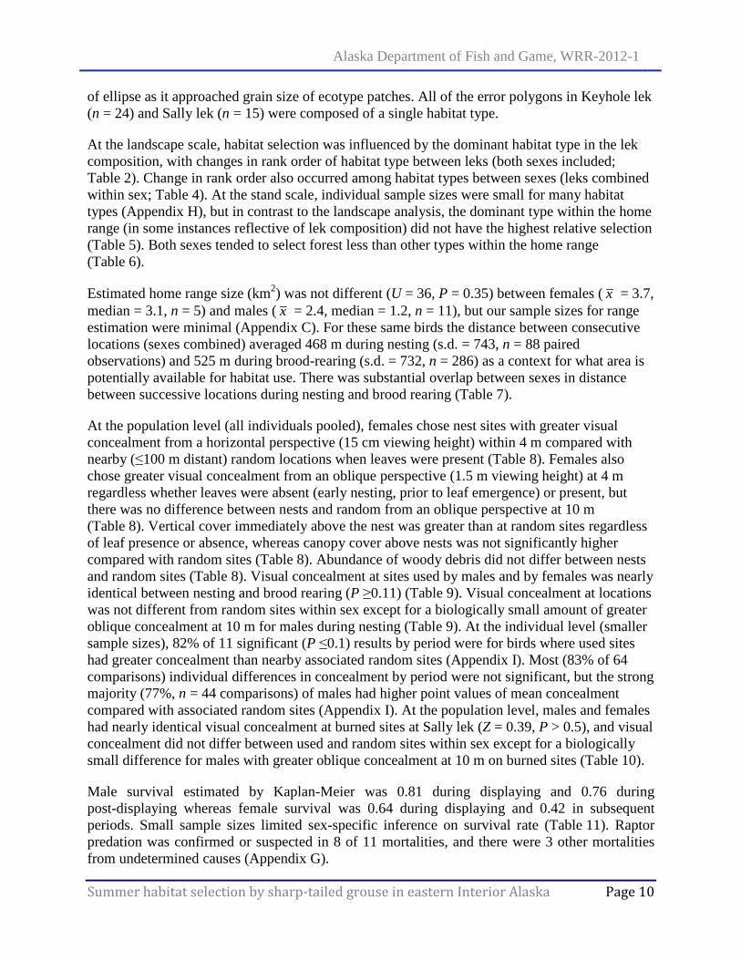
At the population level (all individuals pooled), females chose nest sites with greater visual concealment from a horizontal perspective (15 cm viewing height) within 4 m compared with nearby (≤100 m distant) random locations when leaves were present (Table 8). Females also chose greater visual concealment from an oblique perspective (1.5 m viewing height) at 4 m regardless whether leaves were absent (early nesting, prior to leaf emergence) or present, but there was no difference between nests and random from an oblique perspective at 10 m (Table 8). Vertical cover immediately above the nest was greater than at random sites regardless of leaf presence or absence, whereas canopy cover above nests was not significantly higher compared with random sites (Table 8). Abundance of woody debris did not differ between nests and random sites (Table 8). Visual concealment at sites used by males and by females was nearly identical between nesting and brood rearing (P ≥0.11) (Table 9). Visual concealment at locations was not different from random sites within sex except for a biologically small amount of greater oblique concealment at 10 m for males during nesting (Table 9). At the individual level (smaller sample sizes), 82% of 11 significant (P ≤0.1) results by period were for birds where used sites had greater concealment than nearby associated random sites (Appendix I). Most (83% of 64 comparisons) individual differences in concealment by period were not significant, but the strong majority (77%, n = 44 comparisons) of males had higher point values of mean concealment compared with associated random sites (Appendix I). At the population level, males and females had nearly identical visual concealment at burned sites at Sally lek (Z = 0.39, P > 0.5), and visual concealment did not differ between used and random sites within sex except for a biologically small difference for males with greater oblique concealment at 10 m on burned sites (Table 10).
Male survival estimated by Kaplan-Meier was 0.81 during displaying and 0.76 during post-displaying whereas female survival was 0.64 during displaying and 0.42 in subsequent periods. Small sample sizes limited sex-specific inference on survival rate (Table 11). Raptor predation was confirmed or suspected in 8 of 11 mortalities, and there were 3 other mortalities from undetermined causes (Appendix G).

Alaska Department of Fish and Game, WRR-2012-1
Summer habitat selection by sharp-tailed grouse in eastern Interior Alaska Page 11
Discussion and Recommendations We were unable to capture our intended sample of 30 females in the study area, which inhibited our ability to evaluate whether habitat selection differed between females that were successful in hatching and fledging broods (n = 4) and females that were unsuccessful in reproduction (n = 1). Our average clutch size of 8.9 for initial nests was substantially lower than 12.3 (n = 34; range: 9–16) in Saskatchewan (Pepper 1972) and 12.1 (n = 36; range: 7–17) in Wisconsin (Hamerstrom 1939). Goddard (2007:8) reported mean clutch size of 11.9 (s.e. = 0.18, n = 45) for initial nests in northern British Columbia. Raymond (2001) found 3 nests in the Delta agricultural project but failed to document clutch size. Lower clutch sizes have obvious implications to recruitment. However, hatching (nest) success was 86%, which was higher than has been reported elsewhere. Hatching success was only 44% (n = 50) in northern British Columbia, where 86% of nest losses were attributed to predators (Goddard 2007). Connelly et al. (1998) reported hatching success for sharp-tailed grouse ranged 50–72% among 3 studies in Idaho and Nebraska. Nest and fledging (brood) success can fluctuate annually based on extrinsic factors such as weather or predator abundance, and Gratson (1988) noted that nest success can be reduced through predation at higher nest densities during peaks in grouse populations. The number of birds in the study area in 2010 was relatively low compared with Raymond (2001) and recent knowledge of sharp-tailed grouse abundance in the area (W. Taylor, personal communication). This could partly explain the relatively high nest success we observed. Further investigation into the nesting ecology of Alaska sharp-tailed grouse is warranted.
Contrasting habitat selection among reproductive females (which demonstrates fitness), non-reproductive females, and males was also confounded by the strong difference in lek habitat composition. Substantial overlap of home ranges within and between sexes on both leks reduced the usefulness of inferring landscape level selection. Flocking behavior of males further confounded independence among individuals at the landscape level. At the stand scale, confounding occurred with site effect based on strong difference in habitat composition between leks. Thus, we were unable to meet the main objective of evaluating habitat selection by female sharp-tailed grouse with broods in the Donnelly Training area. Recommendations for further habitat selection are provided below under Study Design.
Even with modifying the study design to include males by capturing birds of either sex wherever they occurred in the study area, we were unable to evaluate the biological value to sharp-tailed grouse of habitats impacted by human actions (including mechanical disturbance) compared with natural disturbance regimes. However, we were able to evaluate the potential effect of a May 2010 prescribed fire on part of Sally lek. Males used burned sites with greater oblique concealment at 10 m during nesting and brood rearing when compared to nearby random sites, but differences were relatively small (Table 10). We could not assess survival consequence of this apparent selection for cover because male mortality primarily occurred during the display period prior to nesting (Table 11).
IMPACT OF NORTHERN GOSHAWKS ON SHARP-TAILED GROUSE We noted goshawks frequently at leks, including observations of goshawks attacking sharp-tailed grouse, and 8 of 11 predation mortalities in our pilot study were attributable to avian predators. Goshawks were documented feeding on sharp-tailed grouse during the 2010 study as well as during 2011 lek monitoring surveys on DTA. Goshawk predation on sharp-tailed grouse occurs

Alaska Department of Fish and Game, WRR-2012-1
Summer habitat selection by sharp-tailed grouse in eastern Interior Alaska Page 12
in other areas (Ammann 1959, Gratson 1982, Marks and Marks 1987) and other grouse species (e.g., Boag and Schroeder 1992, Rusch et al. 2000).
Goshawk population trends follow the snowshoe hare (Lepus americanus) cycle (Boutin et al. 1995). The snowshoe hare population on our study area was sharply declining in 2010 (J. Mason, Fort Wainwright/Donnelly Training Area, unpublished data), and goshawks may have preyed on sharp-tailed grouse more intensely because of low hare numbers. Prey switching by goshawks in response to declines in preferred prey populations has been documented elsewhere (Doyle and Smith 1994, Younk and Bechard 1994).
Research design should consider potential effects of goshawk predation on sample size. Marks and Marks (1987) observed that goshawks preyed selectively on sharp-tailed grouse fitted with radios on a dorsal “poncho” attachment because of visual and auditory cues and cautioned that survival analysis be avoided in situations where avian predation on marked birds could be potentially significant. We also noticed that radio antennas made an auditory “slap” when hitting the wings of flying sharp-tailed grouse and we reduced shine from acrylic on the radios with course grit sandpaper but not until late in the capture period. Regardless of the potential bias to our survival estimates, the incidence of predation during the display period is consistent with observations made elsewhere. Literature reviews show that survival rates for breeding females during spring are relatively low (Bergerud 1988) but <5% of radiomarked hens died on a nest (Bergerud and Gratson 1988).
LOGISTICS OF STUDY SITE Access to a study site is an important consideration in project design. The optimal approach maximizes data collection feasibility (e.g., road access for bird capture, ground telemetry, and habitat measurement) with acceptable study design (e.g., random choice of leks for sampling birds, multiple leks for greater inference). We focused on leks with the greatest number of birds that were reasonably accessible during this period of relatively low grouse abundance. It often was most efficient to focus fieldwork on the Keyhole and Sally leks on alternative days.
Potential to trap and mark a larger sample of females (e.g., 30) should be higher before further efforts are put into a study of nesting ecology. Sex ratio of captures at leks is commonly male dominated by nearly 2:1 (Raymond 2001, Goddard et al. 2009), probably because males are more active at leks, present for a longer period of the day (arrive on leks at pre-dawn and either actively display or loaf until midmorning), and present for the entire display period (approximately 1 month). If at least a 2-year study is feasible, a strategy to increase the number of marked females might be to mark chicks of radiomarked females with small glue-on radios in the first year as part of a cause-specific mortality study. Surviving female subadults could be recaptured in autumn, potentially by use of noose poles or dip nets, and marked with adult necklace radios. Raymond (2001) described overwinter survival of subadult females to the following summer, although relocations were too infrequent to estimate survival rate or loss to hunting. Marking subadult females in fall would improve the chance of having some females already marked going into a second year of spring lek.
METHODS Traps should be inspected for stiffness of the funnel cones prior to each use. We experienced initial failure of funnels in the recycled traps because of fatigued chicken wire that failed to
Alaska Department of Fish and Game, WRR-2012-1
Summer habitat selection by sharp-tailed grouse in eastern Interior Alaska Page 13
retain captured birds. Based on a conversation with a sharp-tailed grouse researcher in Wisconsin (J. Severson, Wisconsin Department of Natural Resources, personal communication to E. Neipert), we built funnels from welded wire fencing instead of chicken wire. The sharp edges of the welded wire cones required constant surveillance of the trap for immediate removal of trapped birds, which we did not realize until 3 male grouse were injured (1 fatally, 1 euthanized) by the wire prongs during the one night these funnels were deployed. We immediately replaced them with new chicken wire cones held in place for greater stiffness with 30 cm spikes, which retained captured birds without injury. There is potential to use rocket nets for capture in conducive vegetation (i.e., grassland or low shrub) at times of peak attendance at breeding leks for both sexes (Appendix A) because birds are focused into area ~10–15 m in diameter.
Additional considerations on trap construction:
• Use ≤1.5 inch plastic mesh for the tops and bungees to strap it down. The plastic would be less damaging to the birds jumping to escape, and bungee cords would be faster to mount/dismount than wire twist ties. Fabric mesh might be an option but could sag if not secured tightly. Both these options are lighter and easier to carry than wire mesh. A potential drawback to the plastic is that it could break in the cold since is more brittle than fabric.
• Put a door secured in the side of the trap (pen) to leave open when trap is not in use. Don’t put it opposite the funnel because sometimes traps are put back to back at a set. Birds might become habituated to an open trap, potentially increasing capture rates. The door could be a slightly larger piece of the same or similar welded wire with hog rings for hinges and a bungee cord to secure it open or closed.
• Cover all welded wire on traps with 1" galvanized chicken wire. This would be labor intensive but could largely eliminate depredation of birds in the traps because only a weasel could enter. Use galvanized because it is better camouflaged and lasts longer in the field over time.
Error polygons from telemetry were substantially smaller than average polygon size in the ecotype classification. If future classifications result in similar sized polygons, the extra step of estimating error polygons and extracting cover types from polygons instead of points may have little effect on estimated use of cover types beyond simply the point estimate. We had difficulty using the LOAS software to output shapefiles of error polygons or ellipses with the associated attribute data. Attributes from the separate point files had to be manually matched with polygons and ellipses in the GIS, greatly increasing data handling time. We contacted the manufacturer, who confirmed our data performed properly and provided a free updated version of the software. By then our work was finished, but this problem correction should be verified before further work is done.
Because spatial error influences habitat selection inference (Montgomery et al. 2011), data from this study could be used to estimate the effect of angular error in telemetry bearings and its variation for empirical adjustment of the maximum likelihood estimator in LOAS software. In the pilot study we used a constant of 2 s.d. (default in program) for expediency in estimating the error polygon when only 2 bearings were useful, which reduced the size of the estimated error

Alaska Department of Fish and Game, WRR-2012-1
Summer habitat selection by sharp-tailed grouse in eastern Interior Alaska Page 14
(area) by more than an order of magnitude in some instances. Our pilot data could allow angular error to be estimated for the study area by observer or for all observers combined for future studies where estimating location error is important. Attempting 3 bearings and plotting on field maps to ensure tight convergence should remain the standard protocol.
Our grouping of ecotypes into a small subset for computational purposes is broadly instructive of habitat selection with an available classification but is not adequate for linking specific traits to fitness. It masks the ecological parameters associated with predation risk (e.g., visual cover) and forage abundance. For example, our habitat measurements indicated that females chose nest sites with greater vertical cover than random sites ≤100 m from the nest (Table 8). Failure to uncover mechanistic covariates of fitness will reduce the potential to translate findings from this study area to other similar situations in Interior Alaska or other regions of the boreal forest. Based on observations of postbreeding fidelity by males to sites with an abundance of overwintered kinnikinnik fruit, future studies of habitat selection should consider techniques to estimate soft mast and possibly insect abundance in selected habitat types.
Our measurement of habitat physical structure at random sites was spatially conservative (≤100 m radius of actual locations, by individual) compared with average distance moved by birds between relocations (ca. 500 m). Researchers in northeast British Columbia chose 250 m radius for evaluating habitat use in aspen-white spruce (Picea glauca) forest and farmland (Goddard et al. 2009). We chose the conservative 100 m prior to knowing relocation movement distances as a reasonable compromise for foot travel in the field. This distance is also close in scale to ecotype patch size in both leks. Our sampling areas and uneven distribution of marked birds by sex did not allow comparison of habitat structure between natural disturbances (primarily upland fire or fluvial action) and human disturbances (prescribed fire, mechanical clearing, and bison forage plots). This type of comparison could be instructive in determining whether the type or frequency of disturbances (human vs. natural) has a different influence on success in brood rearing (e.g., susceptibility to predation). The rotation period for vegetation management is an important variable if the intent is to maintain a site with less cover (e.g., hazardous fuel).
Inference on the selection analysis is complex to interpret for such a small number of individuals where strong habitat differences between leks likely influence site factors (e.g., predation risk or forage abundance) that likely confound patterns of sex-based selection, which is the desired inference. Further analysis could include dropping rare habitats that are rarely used (or never found and never used for some birds), such as low scrub in Keyhole and forest in Sally, to see if substantial changes in rank order or mean index value would occur. Pooling of rare types to reduce experiment-wise error is not feasible because rare types differ between leks. More thoughts on what are being represented by the raw use values and the selection indices are warranted before making final recommendations on future study design. Strong variation in home range size among individuals within sex in each lek (Figs. 2 and 3, Appendix C) warrants closer examination of selection among types for specific individuals that might help plan future work. It would be instructive to examine covariates of specific habitat types (e.g., forage abundance) and to better understand specific behaviors influencing habitat selection or activity centers.

Alaska Department of Fish and Game, WRR-2012-1
Summer habitat selection by sharp-tailed grouse in eastern Interior Alaska Page 15
The ecotype classification from 1994 imagery (Jorgenson et al. 2001) had substantial validation but lacked a vegetative structural component important to inference on concealment cover for sharp-tailed grouse. The National Land Cover Database uses Landsat imagery from 2001 (http://www.mrlc.gov/nlcd2001.php), but type classes were not specific to Alaska, and validation at the scale and location of DTA was likely minimal. Army foresters had begun validating portions of DTA to Level IV in the Alaska Vegetation Classification (Viereck et al. 1992), which includes structural class and understory composition. The portion of the 1999 burn that contains Keyhole lek and adjacent sections of private lands had not been reclassified when this pilot study began. In late summer 2011, the military contracted with the Salcha-Delta area Soil and Water Conservation District (SWCD) to finish a classification of DTA to Viereck Level IV including the area with Keyhole lek. However, this classification does not have an error assessment (W. Wright, SWCD, personal communication, email 13 September 2011). We extracted MCP, polygon, ellipse, and point locations from this Viereck classification for analysis in this report. Type composition from the Viereck classification (Appendix J) was substantially different within each lek from the indirect categorization of ecotype classification to Viereck Level I or II for this report, except for forest (Table 2). Without an error matrix for the Viereck classification, we cannot assess its accuracy compared with our indirect method in describing vegetation.
STUDY DESIGN Understanding population dynamics and importance of habitats used by sharp-tailed grouse in DTA will ideally require study at the scale of the vegetation-disturbance matrix that includes both DTA and the adjacent Delta agricultural project to identify potential existence of population sources and sinks (Pulliam 1988). Raymond (2001:26) showed winter range use by birds marked in the agricultural area that overlapped both composite MCPs at leks in the DTA study area. Attempting to infer effects of vegetation management practices on grouse habitat use or reproductive success in either area in isolation of the other could lead to spurious conclusions if there is substantial exchange of individuals between the 2 areas among years.
Broader inference on whether the nesting and brood rearing habitat associated with Sally and Keyhole leks is representative of DTA or comparatively unique would be instructive to understanding criteria for habitat conservation. In April we searched the eastern DTA and adjacent agricultural project for leks based on past knowledge. A future project could estimate vegetative composition within 1.6 km of known leks (contained female nesting and brood rearing in this study) and calculate selection indices relative to vegetative composition of DTA and the agricultural project. This analysis might include inference on physical covariates of leks (e.g., elevation or distance from recent vegetative disturbance) to identify other potential leks nearby areas to search for evidence of display behavior. Human displacement of birds from leks by permanent occupation (infrastructure development) or repeated disturbance during the display period could negatively influence fitness of individuals through disruption of breeding success. The extent of this concern depends on whether the small number of confirmed leks in the study area and relatively close proximity of nesting and brood rearing to leks represent the best habitat for survival and recruitment to the breeding population. Alternatively, birds in the Tanana Valley have shown use of human disturbed areas for display grounds (e.g., Buffalo Drop Zone on DTA), including active agricultural fields (Kessel 1981, personal communication with S. DuBois, ADF&G, Delta) along roads (Weeden 1965:72), and even along highways when presumably displaced from leks by sudden snowfall (S. DuBois, personal communication).

Alaska Department of Fish and Game, WRR-2012-1
Summer habitat selection by sharp-tailed grouse in eastern Interior Alaska Page 16
Baydack and Hein (1987) tested several disturbance factors on sharp-tailed grouse leks in Manitoba (vehicles, snow fence, leashed dog, scarecrow with voice recordings, radio sound) and found that males exhibited strong fidelity to leks in spring and fall and tolerated a wide range of disturbance without abandoning use of leks. Only the presence of humans dissuaded use by males, but males returned immediately after humans departed. In contrast, females were affected to some extent by all types of disturbance, which precluded breeding on manipulated leks. If undisturbed lek sites are absent in the area or of lower quality (i.e., higher predation risk or other pertinent factor), the result could be a potential decrease in abundance of sharp-tailed grouse in the area.
Occupancy and abundance of birds varies among those leks active in 2010 and other leks with historic and present (2011) use in DTA (W. Taylor, unpublished data). Ultimately the value of specific leks would need to be confirmed by measuring fitness of individuals associated with specific leks and understanding whether differences in nesting rate and brood rearing success were caused by annual factors that vary across the landscape (e.g., forage abundance) or longer term features of habitat type potentially affected by humans (e.g., structure of cover affording concealment from predators in ephemeral early seres compared with natural climax seres, interspersion of habitats and their scale, etc.). If habitat selection by sharp-tailed grouse is preemptive (occupancy of specific habitat types by one reproductive female restricts occupancy by another), increasing density in preferred habitats may limit further population growth if the preferred habitats are locally rare (Pulliam and Danielson 1991).
Habitat selection by individuals (Design 3; Thomas and Taylor 2006) or the density of individuals that occupy a habitat type are indications of habitat importance to life requisites for a species, but fitness is the ultimate validation of critical habitat (Van Horne 1983). Future study of fitness across leks and estimating habitat selection at that order of landscape scale may be sufficient to evaluate effects of land management in DTA on sharp-tailed grouse fitness. Going to finer levels of habitat selection on individual birds requires substantial labor in the field (adequate relocations to estimate home ranges and selection indices by individual bird, visiting used and random sites to assess covariates) and office (grouping of habitat types in classification, telemetry data entry, estimation of point location and error ellipses/polygons, extraction of habitat points and polygons, and comparing use and availability for estimating selection). Simulations by Alldredge and Ratti (1986) recommended sample sizes of at least 20 animals with 50 observations per animal to determine resource selection for a population during a season. This sample size of observations per animal is warranted for sharp-tailed grouse in Interior Alaska based on our area-observation curves for calculating MCP home ranges (Appendix C) and low sample size per habitat type (Appendix H) even after grouping to reduce number of pairwise comparisons. Having use categories estimated with low samples sizes (e.g., 1–6% of total) is problematic in selection studies (Thomas and Taylor 2006).
Alternatively, estimating fitness by lek would require radiomarking a much larger sample of hens among several leks and periodically determining hatch success, brood survival, and fledging by telemetry-aided observation. Further inquiry into whether this would ideally require radiomarking chicks (expensive and labor intensive) or use of trained dogs for brood surveys would be warranted. Following broods would require potentially multiple crews in an intense effort of lek trapping and radiomarking females in spring with subsequent female telemetry and brood observation by a single crew in summer. Assessing sharp-tailed grouse fitness

Alaska Department of Fish and Game, WRR-2012-1
Summer habitat selection by sharp-tailed grouse in eastern Interior Alaska Page 17
simultaneously in DTA and adjacent agricultural land and forested matrix to the northeast would be instructive, particularly to compare nesting and brood rearing success between areas under various management options (active agriculture, fallow in rotation, fallow reverting to forest in Conservation Reserve Program, prescribed fire, mowed/brush-hogged, etc.) with nonmanipulated lands. If remotely sensed metrics of vegetation cover (e.g., vertical structure, stem density, cover) on leks can be correlated to sharp-tailed grouse fitness, this type of information would be more useful to managers planning mitigation of vegetation disturbance than an aspatial mechanistic understanding of fitness (e.g., forage abundance). Regardless, the challenge of accessing multiple leks and capturing an adequate sample of females in spring will likely be the primary limitation in this study area. Specific questions regarding land management decisions (e.g., potential effect on sharp-tailed grouse of modifying vegetation in a specific habitat type or on a known lek) and the desired level of inference (chance of making an incorrect decision that could reduce breeding success on a lek and potentially reduce sharp-tailed grouse abundance on DTA) should be discussed with a biometrician when planning future studies so logistic and sample size requirements are clearly defined.
HABITAT MANAGEMENT AND HUMAN-CAUSED DISTURBANCE Giesen and Connelly (1993) provide guidelines for maintaining sharp-tailed grouse habitat capability in southern subspecies that discuss factors pertinent to consider in field studies for the Alaska subspecies. Mitigating direct disturbance (e.g., human activity on or near an active lek) during the breeding display period may be more important than habitat features alone. In lieu of further field studies to assign fitness of sharp-tailed grouse to specific habitat types in DTA, we should assume the reproductive component of fitness is represented by consistently or heavily used leks (Giesen and Connelly 1993). These authors recommended that disturbance at leks by physical, mechanical, or audible means should be avoided within 3 hours of sunrise and sunset during the breeding season (late March to early June). Peak display occurs from mid-April to mid-May near Delta (W. Taylor, unpublished report, 2010).
Sites with recently disturbed native vegetation seemed to function as displaying grounds near Delta (Kessel 1981), presumably as long as human activity or other disturbance does not disrupt lek activity (Baydack and Hein 1987). Prescribed fire to mitigate hazardous fuels should ideally occur prior to commencement of peak lek use in mid-April to avoid disruption of breeding and certainly prior to mid-May to avoid destruction of nests. Prescribed fire would be less of a temporal conflict in years of low snow accumulation that allow fine fuels to dry earlier in spring (grouse display activity is presumably entrained to photoperiod although affected daily by weather). Giesen and Connelly (1993) defined a 2 km radius around leks as the breeding complex and recommended that vegetative manipulation be avoided in this area to avoid potentially reducing cover used during nesting and brood rearing. The 7 nests we documented were ≤1.3 km from their associated breeding leks, and 4 females observed with broods were ≤1.6 km from associated leks. Although fire or mechanical treatments on vegetation may actually increase potential lek habitat near Delta, we recommend avoiding human-caused disturbance at existing leks during breeding to minimize displacement of females and avoiding extensive vegetative disturbance within 2 km of existing leks to maintain cover for nesting and brood rearing.

Alaska Department of Fish and Game, WRR-2012-1
Summer habitat selection by sharp-tailed grouse in eastern Interior Alaska Page 18
Acknowledgments John Haddix conceived the study, facilitated communication with the U.S. Army, and provided field support. William Taylor, DVM, trained capture crews and generously offered insights on grouse ecology from his past experience in the study area. Elizabeth Neipert coordinated capture logistics, assisted with data collection and management, and edited the final report. Steve DuBois provided logistic support at the Delta Fish and Game office. We thank the following people for intellectual engagement and diligent fieldwork: Joe Ceradini, Janelle Curtis, Jeff Dacey, Adam DuBour, Elizabeth Goldsmith, Brandon Haslick, Mark Kurzen, Micah Miller, Aleya Nelson, Kurt Schmidt, and Jeff Wells. Dr. Stephen Arthur estimated area-observation curves from telemetry data and provided advice on interpretation of selection indices. This report fulfills contract W912CZ-08-D-0012, Delivery Order #7 to U.S. Army Alaska.
Literature Cited Alldredge, J. R., and J. T. Ratti. 1986. Comparison of some statistical techniques for analysis of
resource selection. Journal of Wildlife Management 50:157–165
Ammann, G. A. 1959. Sharp-tailed grouse predation by goshawk. Journal of Wildlife Management 23:110–111.
Baydack, R. K., and D. A. Hein. 1987. Tolerance of sharp-tailed grouse to lek disturbance. Wildlife Society Bulletin 15:535–539.
Bergerud, A. T. 1988. Population ecology of North American grouse. Pages 578–685 in A. T Bergerud and M. W. Gratson, editors. Adaptive strategies and population ecology of northern grouse. University of Minnesota Press, Minneapolis.
Bergerud, A. T., and M. W. Gratson. 1988. Survival and breeding strategies of grouse. Pages 473–577 in A. T. Bergerud and M. W. Gratson, editors. Adaptive strategies and population ecology of northern grouse. University of Minnesota Press, Minneapolis.
Block, W. M, and L. A. Brennan. 1993. The habitat concept in ornithology: Theory and applications. Pages 35–91 in D. M. Power, editor. Current Ornithology. Volume 11. Plenum Press, New York.
Boag, D. A., and M. A. Schroeder. 1992. Spruce grouse (Falcipennis canadensis). In The birds of North America online. A. Poole, editor. Cornell Lab of Ornithology, Ithaca, New York. http://bna.birds.cornell.edu/bna/species/005 (Accessed 8 February 2012).
Boutin, S., C. J. Krebs, R. Boonstra, M. R. T. Dale, S. J. Hannon, K. Martin, A. R. E. Sinclair, J. N. M. Smith, R. Turkington, M. Blower, A. Byrom, F. I. Doyle, C. Doyle, D. Hik, L. Hofer, A. Hubbs, T. Karels, D. L. Murray, V. Nams, M. O’Donoghue, C. Rohner and S. Schweiger. 1995. Population changes of the vertebrate community during a snowshoe hare cycle in Canada’s boreal forest. Oikos 74:69–80.
Boyce, M. S. 2006. Scale for resource selection function. Diversity and Distributions 12:269–276.
Collins, W. B., and E. F. Becker. 2001. Estimation of horizontal cover. Journal of Range Management 54:67–70.
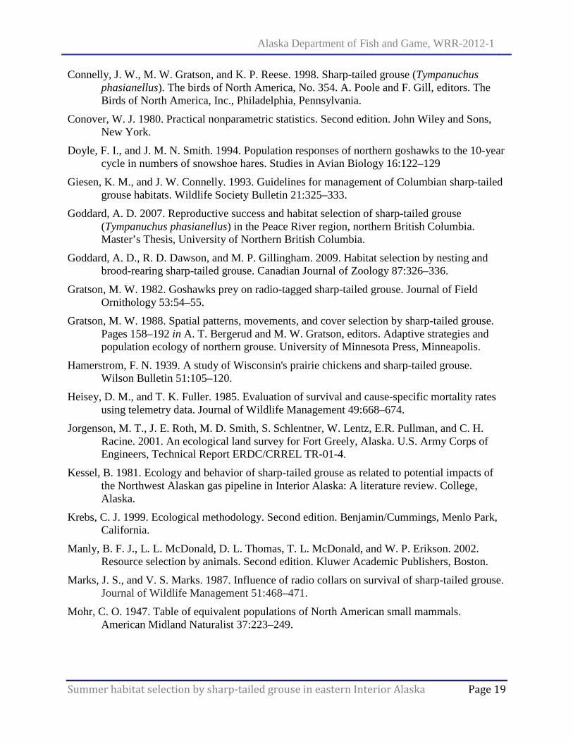
Alaska Department of Fish and Game, WRR-2012-1
Summer habitat selection by sharp-tailed grouse in eastern Interior Alaska Page 19
Connelly, J. W., M. W. Gratson, and K. P. Reese. 1998. Sharp-tailed grouse (Tympanuchus phasianellus). The birds of North America, No. 354. A. Poole and F. Gill, editors. The Birds of North America, Inc., Philadelphia, Pennsylvania.
Conover, W. J. 1980. Practical nonparametric statistics. Second edition. John Wiley and Sons, New York.
Doyle, F. I., and J. M. N. Smith. 1994. Population responses of northern goshawks to the 10-year cycle in numbers of snowshoe hares. Studies in Avian Biology 16:122–129
Giesen, K. M., and J. W. Connelly. 1993. Guidelines for management of Columbian sharp-tailed grouse habitats. Wildlife Society Bulletin 21:325–333.
Goddard, A. D. 2007. Reproductive success and habitat selection of sharp-tailed grouse (Tympanuchus phasianellus) in the Peace River region, northern British Columbia. Master’s Thesis, University of Northern British Columbia.
Goddard, A. D., R. D. Dawson, and M. P. Gillingham. 2009. Habitat selection by nesting and brood-rearing sharp-tailed grouse. Canadian Journal of Zoology 87:326–336.
Gratson, M. W. 1982. Goshawks prey on radio-tagged sharp-tailed grouse. Journal of Field Ornithology 53:54–55.
Gratson, M. W. 1988. Spatial patterns, movements, and cover selection by sharp-tailed grouse. Pages 158–192 in A. T. Bergerud and M. W. Gratson, editors. Adaptive strategies and population ecology of northern grouse. University of Minnesota Press, Minneapolis.
Hamerstrom, F. N. 1939. A study of Wisconsin's prairie chickens and sharp-tailed grouse. Wilson Bulletin 51:105–120.
Heisey, D. M., and T. K. Fuller. 1985. Evaluation of survival and cause-specific mortality rates using telemetry data. Journal of Wildlife Management 49:668–674.
Jorgenson, M. T., J. E. Roth, M. D. Smith, S. Schlentner, W. Lentz, E.R. Pullman, and C. H. Racine. 2001. An ecological land survey for Fort Greely, Alaska. U.S. Army Corps of Engineers, Technical Report ERDC/CRREL TR-01-4.
Kessel, B. 1981. Ecology and behavior of sharp-tailed grouse as related to potential impacts of the Northwest Alaskan gas pipeline in Interior Alaska: A literature review. College, Alaska.
Krebs, C. J. 1999. Ecological methodology. Second edition. Benjamin/Cummings, Menlo Park, California.
Manly, B. F. J., L. L. McDonald, D. L. Thomas, T. L. McDonald, and W. P. Erikson. 2002. Resource selection by animals. Second edition. Kluwer Academic Publishers, Boston.
Marks, J. S., and V. S. Marks. 1987. Influence of radio collars on survival of sharp-tailed grouse. Journal of Wildlife Management 51:468–471.
Mohr, C. O. 1947. Table of equivalent populations of North American small mammals. American Midland Naturalist 37:223–249.

Alaska Department of Fish and Game, WRR-2012-1
Summer habitat selection by sharp-tailed grouse in eastern Interior Alaska Page 20
Montgomery, R. A., G. J. Roloff, and J. M. Ver Hoef. 2011. Implications of ignoring telemetry error on inference in wildlife resource use models. Journal of Wildlife Management 75:702–708.
Odum, E. P., and E. J. Kuenzler. 1955. Measurement of territory and home range size in birds. Auk 72:128–137.
Pepper, G. W. 1972. The ecology of sharp-tailed grouse during spring and summer in the aspen parklands of Saskatchewan. Saskatchewan Department of Natural Resources, Wildlife Report 1.
Pollock, K. H., C. R. Winterstein, C. M. Bunck, and P. D. Curtis. 1989. Survival analysis in telemetry studies: the staggered entry design. Journal of Wildlife Management 53:7–15.
Preston, D. J. 1983. The impacts of agriculture on wildlife. Alaska Department of Fish and Game. Federal Aid in Wildlife Restoration, Final Research Report, Projects W-21-2 and W-21-1, Job 18.6R, Juneau, Alaska.
Pulliam, H. R. 1988. Sources, sinks, and population regulation. American Naturalist 132:652–661.
Pulliam, H. R., and B. J. Danielson. 1991. Sources, sinks, and habitat selection: a landscape perspective on population dynamics. American Naturalist 137 (Supplement):S50–S66.
Raymond, R. L. 2001. Use of summer and winter habitat by Alaska sharp-tailed grouse (Tympanuchus phasianellus caurus) in eastern Interior Alaska. Master’s Thesis, Alaska Pacific University, Anchorage, Alaska.
Rosenberg, D. K., and K. S. McKelvey. 1999. Estimation of habitat selection for central-place foraging animals. Journal of Wildlife Management 63:1028–1038.
Rusch, D. H., S. Destefano, M. C. Reynolds, and D. Lauten. 2000. Ruffed grouse (Bonasa umbellus). The birds of North America online. A. Poole, editor. Cornell Lab of Ornithology, Ithaca, New York. http://bna.birds.cornell.edu/bna/species/515 (Accessed 8 February 2012).
Schroeder, M. A., and C. E. Braun. 1991. Walk-in traps for capturing greater prairie-chickens on leks. Journal of Field Ornithology 62:378–385.
Seefeldt, S. S., J. S. Conn, M. Zhang, and P. N. Kaspari. 2010. Vegetation changes in Conservation Reserve Program lands in Interior Alaska. Agriculture, Ecosystems and Environment 135:119–126.
Thomas, D. L., and E. J. Taylor. 2006. Study designs and tests for comparing resource use and availability II. Journal of Wildlife Management 70:324–336.
U.S. Army Corps of Engineers. 2005. Method to estimate vegetative cover on Army training lands. Public Works Technical Bulletin 200-1-37, Washington, D.C.
U.S. Army Garrison Alaska. 2007a. 2007–2011 Integrated natural resources management plan. Volume II, Annex C, Forestry and Wildland Fire Management. Updated 25 September 2009. http://www.usarak.army.mil/conservation/INRMP_Final/USAGAK_INRMP_07-11_volume_II_annex_C_forestry.pdf (Accessed 8 February 2012).

Alaska Department of Fish and Game, WRR-2012-1
Summer habitat selection by sharp-tailed grouse in eastern Interior Alaska Page 21
U.S. Army Garrison Alaska. 2007b. 2007–2011 Integrated natural resources management plan. Volume II, Annex D, Fish and Wildlife Management. Updated 25 September 2009. http://www.usarak.army.mil/conservation/INRMP_Final/USAGAK_INRMP_07-11_volume_II_annex_D_fish_and_wildlife.pdf (Accessed 8 February 2012).
Van Horne, B. 1983. Density as a misleading indicator of habitat quality. Journal of Wildlife Management 47:893–901.
Verbyla, D. L. 2002. Practical GIS analysis. Taylor and Francis, New York.
Viereck, L. A., C. T. Dyrness, A. R. Batten, and K. J. Wenzlick. 1992. The Alaska vegetation classification. General Technical Report PNW-GTR-286. Portland, OR: U.S. Department of Agriculture, Forest Service, Pacific Northwest Research Station.
Weeden, R. B. 1965. Grouse and ptarmigan in Alaska: Their ecology and management. Alaska Department of Fish and Game. Federal Aid in Wildlife Restoration, Volume V, Project W-6-R-5, Work Plan I. Juneau, Alaska.
White, G. C., and R. A. Garrott. 1990. Analysis of wildlife radio-tracking data. Academic Press, New York.
Younk, J. V., and M. J. Bechard. 1994. Breeding ecology of the northern goshawk in high elevation aspen forests of northern Nevada. Studies in Avian Biology 16:119–128.
Zar, J. H. 1984. Biostatistical analysis. Second edition. Prentice-Hall, Englewood Cliffs, New Jersey.
Zar, J. H. 1999. Biostatistical analysis. Fourth edition. Prentice-Hall, Englewood Cliffs, New Jersey.

Alaska Department of Fish and Game, WRR-2012-1
Summer habitat selection by sharp-tailed grouse in eastern Interior Alaska Page 22
Figure 1. Location of breeding leks, nest sites, and composite ranges for all locations of sharp-tailed grouse (STGR) on the Donnelly Training Area, Alaska, May–September 2010.

Page 23
Alaska D
epartment of Fish and G
ame, W
RR
-2012-1
Summ
er habitat selection by sharp-tailed grouse in eastern Interior Alaska
Figure 2. Location of 100% minimum convex polygon (MCP) home ranges of male and female sharp-tailed grouse on Keyhole lek, Donnelly Training Area, Alaska, May–September 2010.
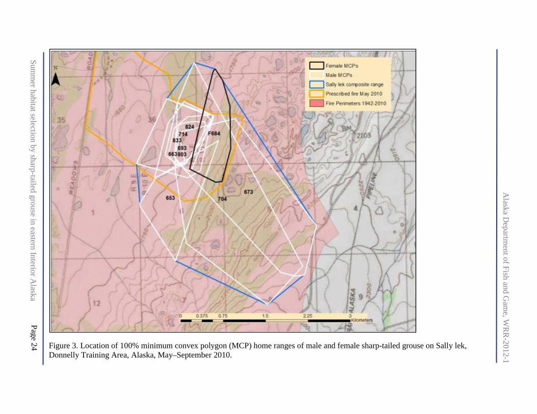
Page 24
Alaska D
epartment of Fish and G
ame, W
RR
-2012-1
Summ
er habitat selection by sharp-tailed grouse in eastern Interior Alaska
Figure 3. Location of 100% minimum convex polygon (MCP) home ranges of male and female sharp-tailed grouse on Sally lek, Donnelly Training Area, Alaska, May–September 2010.

Alaska Department of Fish and Game, WRR-2012-1
Summer habitat selection by sharp-tailed grouse in eastern Interior Alaska Page 25
Table 1. Estimated date of hatch, clutch size, nest distance from capture lek, and estimated date of brood persistence for female sharp-tailed grouse, Donnelly Training Area, Alaska, 2010.
Hen ID
Lek
Nest discoverya
Hatch
Clutch size
Distance from lek (m)
Last observation of chicks(s)b
573c Keyhole 18 May 5 Jun 10 1020 Depredated at hatch 583 Keyhole 17 May 8 Jun 9 657 6 Sep 684 Sally 17 May 9 Jun 10 1230 6 Sep 724 Keyhole 17 May 7 Jun 8 530 Hen predation ca. 12 Jun 814 Keyhole 24 May 8 Jun 9 530 10 Sep 863 Keyhole 18 May —d 9 1070 —d 863e Keyhole 3 Jun 23 Jun 7 1230 9 Jul
a Nest initiation probably occurred around time of nest discovery except for F814 (incubation is 21–23 days; Connelly et al. 1998:10). b Ability to discern chicks from radiomarked adult (not always observed because of vegetative cover) and onset of chick dispersal inhibited fate assessment for unmarked chicks by late summer. c Original female marked with frequency 573 died on 4 or 5 May, and radio collar was redeployed 7 May to this individual. d Nest failed or was abandoned 18 May because of human or dog disturbance. e Re-nest.
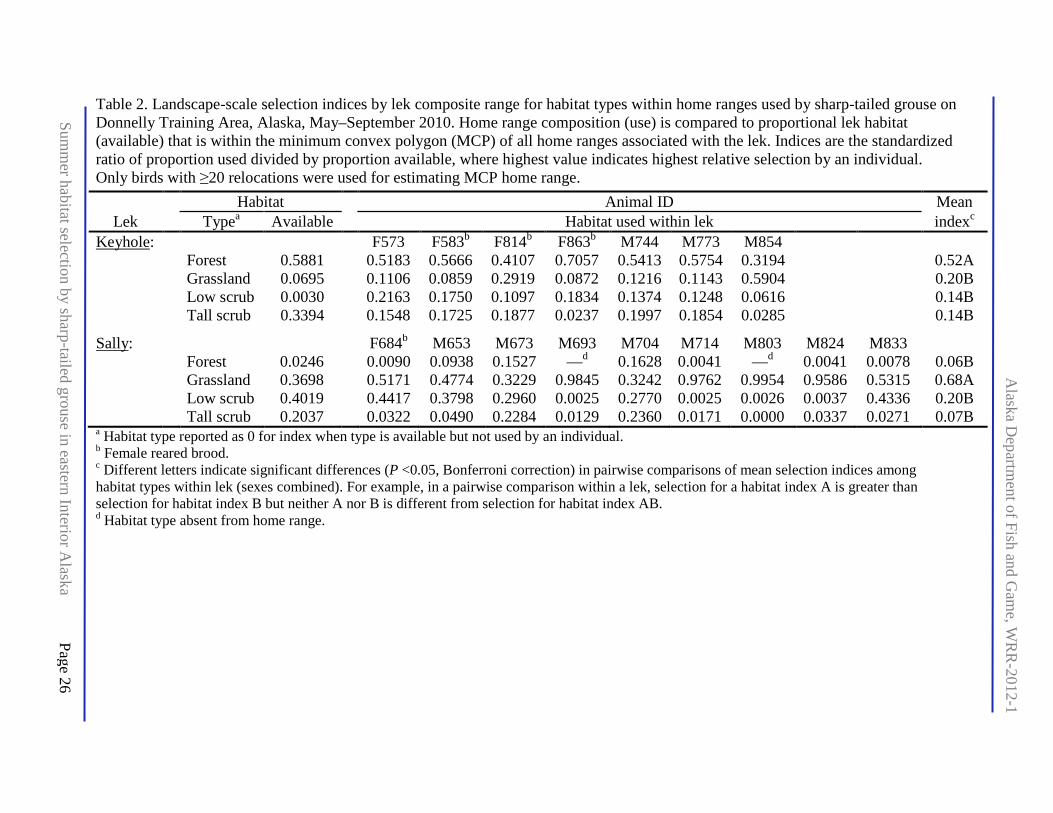
Page 26
Alaska D
epartment of Fish and G
ame, W
RR
-2012-1
Summ
er habitat selection by sharp-tailed grouse in eastern Interior Alaska
Table 2. Landscape-scale selection indices by lek composite range for habitat types within home ranges used by sharp-tailed grouse on Donnelly Training Area, Alaska, May–September 2010. Home range composition (use) is compared to proportional lek habitat (available) that is within the minimum convex polygon (MCP) of all home ranges associated with the lek. Indices are the standardized ratio of proportion used divided by proportion available, where highest value indicates highest relative selection by an individual. Only birds with ≥20 relocations were used for estimating MCP home range.
Habitat Animal ID Mean Lek Typea Available Habitat used within lek indexc
Keyhole: F573 F583b F814b F863b M744 M773 M854 Forest 0.5881 0.5183 0.5666 0.4107 0.7057 0.5413 0.5754 0.3194 0.52A Grassland 0.0695 0.1106 0.0859 0.2919 0.0872 0.1216 0.1143 0.5904 0.20B Low scrub 0.0030 0.2163 0.1750 0.1097 0.1834 0.1374 0.1248 0.0616 0.14B Tall scrub 0.3394 0.1548 0.1725 0.1877 0.0237 0.1997 0.1854 0.0285 0.14B Sally: F684b M653 M673 M693 M704 M714 M803 M824 M833
Forest 0.0246 0.0090 0.0938 0.1527 —d 0.1628 0.0041 —d 0.0041 0.0078 0.06B Grassland 0.3698 0.5171 0.4774 0.3229 0.9845 0.3242 0.9762 0.9954 0.9586 0.5315 0.68A Low scrub 0.4019 0.4417 0.3798 0.2960 0.0025 0.2770 0.0025 0.0026 0.0037 0.4336 0.20B Tall scrub 0.2037 0.0322 0.0490 0.2284 0.0129 0.2360 0.0171 0.0000 0.0337 0.0271 0.07B a Habitat type reported as 0 for index when type is available but not used by an individual. b Female reared brood. c Different letters indicate significant differences (P <0.05, Bonferroni correction) in pairwise comparisons of mean selection indices among habitat types within lek (sexes combined). For example, in a pairwise comparison within a lek, selection for a habitat index A is greater than selection for habitat index B but neither A nor B is different from selection for habitat index AB. d Habitat type absent from home range.

Page 27
Alaska D
epartment of Fish and G
ame, W
RR
-2012-1
Summ
er habitat selection by sharp-tailed grouse in eastern Interior Alaska
Table 3. Extent of error in telemetry relocation of dummy transmitters in a blind test. Variance in angular error for estimating error ellipse with triangulation is empirical, whereas angular error has assumed s.d. = 2 to allow estimation of error polygon with biangulation.
Lek
Trial
Crew
Point error (m)
Error ellipse or polygon (m2)a
Transmitter within error area
Error area and ecotype alikeb
Keyhole Triangulation A 41 1993 No No Keyhole Biangulation A 8 288 Yes Yes Keyhole Biangulation A 51 135 No No Keyhole Triangulation A 3 456 Yes Yes Texas Triangulation B 13 2 No Yes Texas Triangulation B 12 58 No Yes Texas Triangulation B 18 239 No Yes Texas Triangulation B 3 107 Yes Yes a Ecotype resolution 900 m2 in imagery. b Area within error ellipse or polygon has 75–100% of same ecotype (Jorgenson et al. 2001) as dummy transmitter.

Page 28
Alaska D
epartment of Fish and G
ame, W
RR
-2012-1
Summ
er habitat selection by sharp-tailed grouse in eastern Interior Alaska
Table 4. Landscape-scale selection indices by sex for habitat types within home ranges used by sharp-tailed grouse on Donnelly Training Area, Alaska, May–September 2010. Home range composition (use) is compared to proportional lek habitat (available; see Table 2) that within the minimum convex polygon (MCP) of all home ranges associated with the lek. Indices are the standardized ratio of proportion used divided by proportion available, where the highest value indicates the highest relative selection by an individual. Only birds with ≥20 relocations were used for estimating MCP home range.
Sex Habitat type Animal ID Mean
indexc Habitat used by sex Females: F573 F583a F684a F814a F863a
Forest 0.5183 0.5666 0.009 0.4107 0.7057 0.44A Grassland 0.1106 0.0859 0.5171 0.2919 0.0872 0.22AB Low scrub 0.2163 0.175 0.4417 0.1097 0.1834 0.23AB Tall scrub 0.1548 0.1725 0.0322 0.1877 0.0237 0.11B
Males: M653 M673 M693 M704 M714 M744 M773 M803 M824 M833 M854 Forest 0.0938 0.1527 —c 0.1628 0.0041 0.5413 0.5754 —c 0.0041 0.0078 0.3194 0.21B Grassland 0.4774 0.3229 0.9845 0.3242 0.9762 0.1216 0.1143 0.9954 0.9586 0.5315 0.5904 0.58A Low scrub 0.3798 0.296 0.0025 0.277 0.0025 0.1374 0.1248 0.0026 0.0037 0.4336 0.0616 0.16B Tall scrub 0.049 0.2284 0.0129 0.236 0.0171 0.1997 0.1854 0.0055 0.0337 0.0271 0.0285 0.09B
a Female reared brood. b Different letters indicate significant differences (P <0.05, Bonferroni correction) in pairwise comparisons of mean selection indices among habitat type within sex (leks combined). c Habitat type absent from home range.

Page 29
Alaska D
epartment of Fish and G
ame, W
RR
-2012-1
Summ
er habitat selection by sharp-tailed grouse in eastern Interior Alaska
Table 5. Stand-scale selection indices by lek composite range for habitat types within home ranges used by sharp-tailed grouse based on radiotelemetry and observations of marked birds on Donnelly Training Area, Alaska, May–September 2010. Available habitat is composition of home ranges. Indices are the standardized ratio of proportion used divided by proportion available, where the highest value indicates the highest relative selection by an individual. Home range was estimated for birds with ≥20 relocations. Composition of home ranges and selection ratios used to estimate indices are in Appendix H.
Lek Habitat typea
Animal ID Mean indexb Use of available habitat within home range
Keyhole: F573 F583c F814c F863c M744 M773 M854 Forest 0.0696 0.0316 0.0266 0.0103 0.1285 0.1896 0.0405 0.07B Grassland 0.4596 0.6781 0.0689 0.2353 0 0.5385 0 0.28AB Low scrub 0 0 0.8561 0 0 0 0 0.12AB Tall scrub 0.4708 0.2903 0.0483 0.7544 0.8715 0.2719 0.9595 0.52A
Sally: F684c M653 M673 M693 M704 M714 M803 M824 M833 Forest 0 0 0 —d 0 0 —d 0 0 -- Grassland 0.0572 0.1839 0.1636 0.0215 0.1284 0.0145 0.0272 0.0135 0.0000 0.07B Low scrub 0.0534 0.0654 0.1368 0.4535 0.3111 0.3276 0 0.8121 0.0364 0.27AB Tall scrub 0.8894 0.7506 0.6996 0.5249 0.5605 0.6579 0.9728 0.1744 0.0224 0.58A
a Habitat type reported as 0 for index when type is available but not used by an individual. b Different letters indicate significant differences (P <0.05, Bonferroni correction) in pairwise comparisons of mean selection indices among habitat type within lek (sexes combined). c Female reared brood. d Habitat type absent from home range.

Page 30
Alaska D
epartment of Fish and G
ame, W
RR
-2012-1
Summ
er habitat selection by sharp-tailed grouse in eastern Interior Alaska
Table 6. Stand-scale selection indices by sex for habitat types within home ranges used by sharp-tailed grouse based on radiotelemetry and observations of marked birds on Donnelly Training Area, Alaska, May–September 2010. Available habitat is composition of home ranges. Indices are the standardized ratio of proportion used divided by proportion available, where the highest value indicates the highest relative selection by an individual. Home range was estimated for birds with ≥20 relocations. Composition of home ranges and selection ratios used to estimate indices are in Appendix H.
Sex
Habitat typea
Animal ID Mean indexb Use of available habitat within home range by sex
Females: F573 F583c F684c F814c F863c Forest 0.0696 0.0316 0 0.0266 0.0103 0.03B Grassland 0.4596 0.6781 0.0572 0.0689 0.2353 0.30A Low scrub 0 0 0.0534 0.8561 0 0.18AB Tall scrub 0.4708 0.2903 0.8894 0.0483 0.7544 0.49A
Males: M653 M673 M693 M704 M714 M744 M773 M803 M824 M833 M854 Forest 0 0 —d 0 0 0.1285 0.1896 —d 0 0 0.0405 0.04B Grassland 0.1839 0.1636 0.0215 0.1284 0.0145 0 0.5385 0.0272 0.0135 0.0000 0 0.10B Low scrub 0.0654 0.1368 0.4535 0.3111 0.3276 0 0 0 0.8121 0.0364 0 0.21AB Tall scrub 0.7506 0.6996 0.5249 0.5605 0.6579 0.8715 0.2719 0.9728 0.1744 0.0224 0.9595 0.59A
a Habitat type reported as 0 for index when type is available but not used by an individual. b Different letters indicate significant differences (P <0.05, Bonferroni correction) in pairwise comparisons of mean selection indices among habitat type within sex (leks combined). c Female reared brood. d Habitat type absent from home range.

Page 31
Alaska D
epartment of Fish and G
ame, W
RR
-2012-1
Summ
er habitat selection by sharp-tailed grouse in eastern Interior Alaska
Table 7. Distance (m) between successive locations for sharp-tailed grousea estimated during nesting and brood rearing on Donnelly Training Area, Alaska, May–September 2010.
Female (n = 5) Male (n = 11)
Period Range of no. sample pairs
Grand mean
Grand median
Range of means
Range of no. sample pairs
Grand mean
Grand median
Range of means
Nesting 2–7 506 489 264–974 2–6 565 349 158–1674 Rearing 20–24 534 504 393–798 10–17 474 391 228–810 Combined 23–30 519 503 373–675 16–22 493 415 241–887 a Individual birds were the experimental unit with replicate distance measures per individual. Distributions of mean distance moved were non-normal (Lilliefors test, P <0.05) for 69% of the 16 birds, so individual bird movements were plotted as a density distribution (Appendix K) to illustrate variation in the population.

Alaska Department of Fish and Game, WRR-2012-1
Summer habitat selection by sharp-tailed grouse in eastern Interior Alaska Page 32
Table 8. Mean (median in parentheses) visual concealment (%), vertical cover over nest bowl (%), canopy cover (%), and abundance of woody debris pieces at 7 nests used by 6 sharp-tailed grouse females (Table 1) and 3 random sites ≤100 m from each nest (n = 21), Donnelly Training Area, Alaska, 2010. Measurements were made after hatch when foliage was present (“leaf on” simulates late incubation) and after foliage had senesced or dropped in early fall (“leaf off” simulates early incubation). Horizontal concealment of visual target from 15 cm height gauges detection by mammalian predators, whereas oblique and vertical concealment from 1.5 m and overhead, respectively, are for avian predators. Test score is 2-sample Mann-Whitney U.
Leaf off period Leaf on period
Used
Random Test score
P
Used
Random
Test score
P
Concealment at 15 cm above ground from 15 cm height and 4 m distance
93.5 (95.8)
79.0 (79.2)
U = 39 0.064 100 (100)
88.5 (95.8)
U = 32 0.013
Concealment at 15 cm above ground from 1.5 m height and 4 m distance
76.2 (70.8)
52.6 (50.0)
U = 27 0.013 91.1 (100)
64.7 (66.7)
U = 28 0.014
Concealment at 1.5 m above ground from 1.5 m height and 10 m distance
37.5 (41.7)
23.2 (20.8)
U = 54 0.298 37.5 (29.2)
27.2 (20.8)
U = 65 0.65
Vertical cover at 50 cm above nest
36.4 (35.0)
4.1 (2.0)
U = 1 <0.001 38.6 (40)
14.7 (8.0)
U = 20 0.004
Canopy cover from 50 cm above nest
17.3 (12.0)
5.7 (2.8)
U = 44 0.115 20.5 (16.3)
5.9 (2.5)
U = 40 0.068
Number woody debris pieces ≤1 m from nest
1.1 (1.0)
0.6 (0)
U = 55 0.26 —a —a —a —a
a Measurements same as leaf off period; see text for definition of debris.
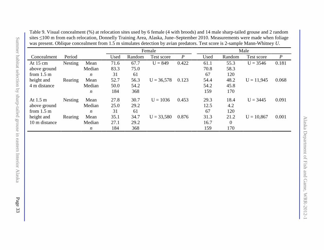
Page 33
Alaska D
epartment of Fish and G
ame, W
RR
-2012-1
Summ
er habitat selection by sharp-tailed grouse in eastern Interior Alaska
Table 9. Visual concealment (%) at relocation sites used by 6 female (4 with broods) and 14 male sharp-tailed grouse and 2 random sites ≤100 m from each relocation, Donnelly Training Area, Alaska, June–September 2010. Measurements were made when foliage was present. Oblique concealment from 1.5 m simulates detection by avian predators. Test score is 2-sample Mann-Whitney U.
Female Male Concealment Period Used Random Test score P Used Random Test score P
At 15 cm above ground from 1.5 m height and 4 m distance
Nesting Mean 71.6 67.7 U = 849 0.422 61.1 55.3 U = 3546 0.181 Median 83.3 75.0 70.8 58.3
n 31 61 67 120 Rearing Mean 52.7 56.3 U = 36,578 0.123 54.4 48.2 U = 11,945 0.068
Median 50.0 54.2 54.2 45.8 n 184 368 159 170
At 1.5 m above ground from 1.5 m height and 10 m distance
Nesting Mean 27.8 30.7 U = 1036 0.453 29.3 18.4 U = 3445 0.091 Median 25.0 29.2 12.5 4.2
n 31 61 67 120 Rearing Mean 35.1 34.7 U = 33,580 0.876 31.3 21.2 U = 10,867 0.001
Median 27.1 29.2 16.7 0 n 184 368 159 170

Alaska D
epartment of Fish and G
ame, W
RR
-2012-1
Summ
er habitat selection by sharp-tailed grouse in eastern Interior Alaska
Page 34
Table 10. Proportion of relocations (used sites) in Sally lek and proportion of 2010 burned area within 10 m radius at used and random sites ≤100 m from each relocation for 1 female with a brood and 8 male sharp-tailed grouse, Donnelly Training Area, Alaska, May–September 2010. Mean and median visual concealment (%) for the same birds when foliage was present is also shown. Oblique concealment from 1.5 m simulates detection by avian predators. Test scores are a 2-sample Z-test for proportions or a 2-sample Mann-Whitney U. Female Male
Used Random Test score P Used Random Test score P Sites visited (n) 46 92 143 190
Sites burned (%) 100 100 87 88
Mean (s.d.) area burned 40.1 (40.4)
34.5 (39.5)
Z = 0.64 P >0.5 43.4 (37.6)
48.8 (39.6)
Z = 0.91 P >0.5
Mean (median) concealment at 15 cm above ground from 1.5 m height and 4 m distance
59.8 (60.4)
61.6 (66.7)
U = 2203 0.695 Burned: 61.6 (70.8)
n = 124
55.2 (62.5)
n = 168
U = 9234 0.097
Not burned: 73.5 (75.0) n = 19
64.2 (68.8) n = 22
U =172 0.337
Mean (median) concealment at 1.5 m above ground from 1.5 m height and 10 m distance
34.1 (27.1)
34.5 (20.3)
U = 2049 0.761 Burned: 18.0 (0)
6.9 (0)
U = 8640 0.003
Not burned: 32.0 (20.8)
16.9 (0)
U = 146 0.065
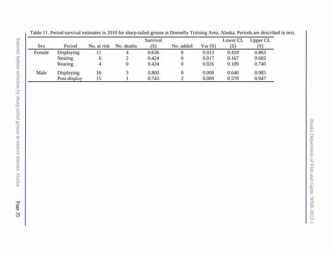
Alaska D
epartment of Fish and G
ame, W
RR
-2012-1
Summ
er habitat selection by sharp-tailed grouse in eastern Interior Alaska
Page 35
Table 11. Period survival estimates in 2010 for sharp-tailed grouse at Donnelly Training Area, Alaska. Periods are described in text.
Sex Period No. at risk No. deaths Survival
(S) No. added Var (S) Lower CL
(S) Upper CL
(S) Female Displaying 11 4 0.636 0 0.013 0.410 0.863
Nesting 6 2 0.424 0 0.017 0.167 0.682 Rearing 4 0 0.424 0 0.026 0.109 0.740
Male Displaying 16 3 0.800 0 0.008 0.640 0.985 Post-display 15 1 0.743 2 0.009 0.570 0.947

Alaska Department of Fish and Game, WRR-2012-1
Summer habitat selection by sharp-tailed grouse in eastern Interior Alaska Page 36
Appendix A. Lek attendance chronology in 2010 by sharp-tailed grouse, Donnelly Training Area, Alaska. Location of leks is shown in Figure 1.
Date Lek name Observation
start time Observation
end time Max. no.
males Max. no. females
Unknown sex Total
4/5/2010 Buffalo DZ 7:45 NA 1 -- 3 4 4/7/2010 Sally DZ 6:40 6:50 0 0 18 18 4/8/2010 Sally DZ 7:08 NA -- -- 23 23 4/8/2010 TX Condo 7:37 9:13 -- -- 9 9 4/9/2010 TX Condo 9:30 NA 3 0 6 9 4/12/2010 Buffalo DZ 8:20 8:35 -- -- 10 10 4/12/2010 Sally DZ 6:42 6:46 2 -- -- 2 4/12/2010 TX Condo 7:05 7:20 -- -- 3 3 4/13/2010 Sally DZ 6:50 NA 12 2 17 31 4/14/2010 1 km S TX Condo 7:00 NA 6+ -- -- 6 4/14/2010 TX Condo 6:05 8:20 -- -- 10 10 4/15/2010 Buffalo DZ 5:30 9:30 2 -- 1 3 4/15/2010 Sally DZ 9:15 9:30 -- -- 18 18 4/15/2010 TX Condo 6:10 9:00 4 3 6 13 4/16/2010 Sally DZ 8:30 NA -- -- 19 19 4/16/2010 TX Condo 6:30 8:20 2 2 1 5 4/20/2010 Buffalo DZ 8:30 9:00 4 1 -- 5 4/21/2010 Sally DZ 7:30 10:00 -- -- 15 15 4/26/2010 Buffalo DZ 6:40 NA 6 1 -- 7 4/27/2010 Keyhole S 5:15 10:30 8 10 -- 18 4/28/2010 Keyhole S 4:55 NA 7 1 -- 8 4/29/2010 Keyhole S 6:00 10:25 7 8 -- 15 5/4/2010 Keyhole N 4:00 6:30 3 2? -- 5 5/4/2010 Keyhole S 4:10 NA 6 3 -- 9 5/5/2010 Keyhole S 4:45 5:00 2 1 -- 3 5/6/2010 Keyhole S 4:25 NA 5 1 -- 6 5/7/2010 Keyhole N 4:10 4:11 1 -- -- 1 5/7/2010 Keyhole S 4:15 9:55 6 1 -- 7 5/10/2010 Keyhole S 4:20 9:30 6 1 -- 7 5/12/2010 Keyhole S 6:45 NA 6 -- -- 6 5/14/2010 Sally DZ 5:00 NA -- -- 14 14 5/17/2010 Sally DZ 5:50 8:00 15 -- -- 15

Alaska Department of Fish and Game, WRR-2012-1
Summer habitat selection by sharp-tailed grouse in eastern Interior Alaska Page 37
Appendix B. Capture dates, radio frequency, sex, and morphometrics of sharp-tailed grouse on Donnelly Training Area, Alaska, 2010.
Cap. event Date
Bird ID
(152 MHz)
Band and leg
Color bands/leg Sex
Wing (mm)
Tarsus (mm)
Wt (g) Lek
Cap. no. Mort
1 13 Apr -- -- Blue Red/R M 207 -- 860 Sally 1 No 2 13 Apr -- -- Blue Red/R M 206 -- 895 Sally 1 No 3 13 Apr -- -- Blue Red/R M 209 -- 945 Sally 1 No 4 13 Apr -- -- Blue Red/R M 214 -- 905 Sally 1 No 5 13 Apr -- -- Blue Red/R M 216 -- 885 Sally 1 No 6 14 Apr -- -- Blue Red/R M 202 -- 805 Sally 1 No 7 15 Apr -- -- Blue Red M -- -- -- Sally 2 No 8 21 Apr 0.623 2/R Blue
Orange/R M 205 99 825 Texas-
Condo N 1 Field
9 21 Apr 0.704 1/R Blue Red/L M 205 102 870 Sally 1 No 10 22 Apr 0.803 3/L Blue Red/R M 210 -- -- Sally
Satellite 1 No
11 22 Apr 0.824 4/L Blue Red/R M 205 -- -- Sally Satellite
1 No
12 22 Apr -- -- -- M -- -- -- 33 Mile Loop
1 Trap
13 23 Apr 0.673 5/R -- M 202 97 -- Texas Condo S
1 No
14 23 Apr 0.824 4/L Blue Red/R M -- -- -- Sally 2 No 15 23 Apr -- -- -- M -- -- -- Sally 1 Trap 16 23 Apr -- -- -- M -- -- -- 33 Mile
Loop 1 Trap
17 24 Apr 0.663 6/R Blue Red/R M 204 105 785 Sally Satellite
1 No
18 24 Apr -- -- -- M -- -- -- Sally 1 Trap 19 25 Apr 0.684 7/R -- F 207 102 670 Sally 1 No 20 26 Apr 0.594 8/R -- M 195 100 780 Keyhole S 1 Field 21 26 Apr 0.744 10/R -- M 205 97 850 Keyhole S 1 No 22 26 Apr 0.773 9/R -- M 198 97 750 Keyhole S 1 No 23 27 Apr 0.583 12/R -- F 200 100 620 Keyhole S 1 No 24 27 Apr 0.614 16/R -- M 199 95.55 720 Keyhole N 1 Field 25 27 Apr 0.634 67/R -- F 194 99 760 Sally 1 Field 26 27 Apr 0.653 35/R -- M 200 99 822 Texas
Condo, N 1 No
27 27 Apr 0.724 11/R -- F 197 97.6 645 Keyhole S 1 No 28 27 Apr 0.763 34/R -- F 199 95 -- Sally 1 Field 29 27 Apr 0.773 9/R -- M -- -- -- Keyhole S 2 No 30 27 Apr 0.783 15/R -- M 197 101.4 760 Keyhole S 1 No 31 27 Apr 0.814 70/R -- F 194 96 690 Keyhole S 1 No 32 27 Apr 0.844 13/R -- M 207 102 710 Keyhole S 1 No 33 27 Apr 0.863 14/R -- F 196 97 675 Keyhole S 1 No 34 27 Apr -- 68/R Blue Red/L M 205 99 870 Sally 1 No 35 27 Apr -- 71/R Yellow
Green/L M 201 95 750 Keyhole S 1 No
36 27 Apr -- -- -- M -- -- -- Sally 1 Trap 37 28 Apr 0.573a 36/R -- F 198 101 880 Sally 1 Field
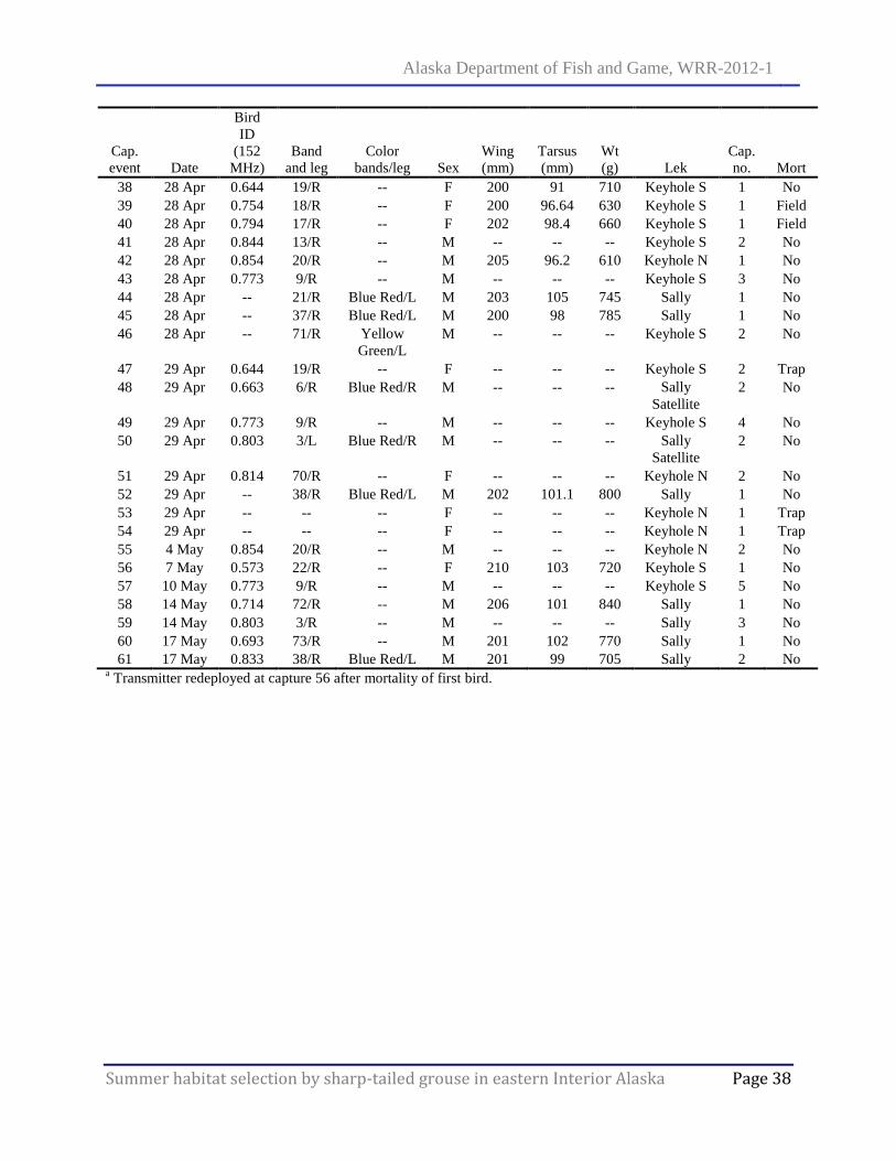
Alaska Department of Fish and Game, WRR-2012-1
Summer habitat selection by sharp-tailed grouse in eastern Interior Alaska Page 38
Cap. event Date
Bird ID
(152 MHz)
Band and leg
Color bands/leg Sex
Wing (mm)
Tarsus (mm)
Wt (g) Lek
Cap. no. Mort
38 28 Apr 0.644 19/R -- F 200 91 710 Keyhole S 1 No 39 28 Apr 0.754 18/R -- F 200 96.64 630 Keyhole S 1 Field 40 28 Apr 0.794 17/R -- F 202 98.4 660 Keyhole S 1 Field 41 28 Apr 0.844 13/R -- M -- -- -- Keyhole S 2 No 42 28 Apr 0.854 20/R -- M 205 96.2 610 Keyhole N 1 No 43 28 Apr 0.773 9/R -- M -- -- -- Keyhole S 3 No 44 28 Apr -- 21/R Blue Red/L M 203 105 745 Sally 1 No 45 28 Apr -- 37/R Blue Red/L M 200 98 785 Sally 1 No 46 28 Apr -- 71/R Yellow
Green/L M -- -- -- Keyhole S 2 No
47 29 Apr 0.644 19/R -- F -- -- -- Keyhole S 2 Trap 48 29 Apr 0.663 6/R Blue Red/R M -- -- -- Sally
Satellite 2 No
49 29 Apr 0.773 9/R -- M -- -- -- Keyhole S 4 No 50 29 Apr 0.803 3/L Blue Red/R M -- -- -- Sally
Satellite 2 No
51 29 Apr 0.814 70/R -- F -- -- -- Keyhole N 2 No 52 29 Apr -- 38/R Blue Red/L M 202 101.1 800 Sally 1 No 53 29 Apr -- -- -- F -- -- -- Keyhole N 1 Trap 54 29 Apr -- -- -- F -- -- -- Keyhole N 1 Trap 55 4 May 0.854 20/R -- M -- -- -- Keyhole N 2 No 56 7 May 0.573 22/R -- F 210 103 720 Keyhole S 1 No 57 10 May 0.773 9/R -- M -- -- -- Keyhole S 5 No 58 14 May 0.714 72/R -- M 206 101 840 Sally 1 No 59 14 May 0.803 3/R -- M -- -- -- Sally 3 No 60 17 May 0.693 73/R -- M 201 102 770 Sally 1 No 61 17 May 0.833 38/R Blue Red/L M 201 99 705 Sally 2 No
a Transmitter redeployed at capture 56 after mortality of first bird.

Alaska Department of Fish and Game, WRR-2012-1
Summer habitat selection by sharp-tailed grouse in eastern Interior Alaska Page 39
Appendix C. Estimated increase in area (km2, y-axis) of minimum convex polygon ranges with increasing number of relocations (x-axis) for 18 sharp-tailed grouse in Donnelly Training Area, Alaska, May–September 2010. Each estimate is the mean of 100 simulations using random selections drawn with replacement for individuals with ≥15 relocations from radiotelemetry. Asymptote indicates a stabilizing range size for the time period examined.
F573 (n = 28)
F583 (n = 39)
0.8
1.3
1.8
2.3
2.8
3.3
10 12 14 16 18 20 22 24 26 28
km2
Number of relocations
1.0
1.2
1.4
1.6
1.8
2.0
2.2
2.4
10 15 20 25 30 35 39
km2
Number of relocations

Alaska Department of Fish and Game, WRR-2012-1
Summer habitat selection by sharp-tailed grouse in eastern Interior Alaska Page 40
F684 (n = 36)
F814 (n = 40)
0.5
0.6
0.6
0.7
0.7
0.8
0.8
0.9
0.9
1.0
10 12 14 16 18 20 22 24 26 30 32 34 36
km2
Number of relocations
0.8
1.0
1.2
1.4
1.6
1.8
2.0
2.2
2.4
10 15 20 25 30 35 40
km2
Number of relocations

Alaska Department of Fish and Game, WRR-2012-1
Summer habitat selection by sharp-tailed grouse in eastern Interior Alaska Page 41
F863 (n = 32)
M653 (n = 20)
0.5
0.6
0.6
0.7
0.7
0.8
0.8
0.9
0.9
10 12 14 16 18 20 22 24 26 30 32
km2
Number of relocations
0.6
0.7
0.8
0.9
1.0
1.1
1.2
1.3
10 12 14 16 18 20
km2
Number of relocations

Alaska Department of Fish and Game, WRR-2012-1
Summer habitat selection by sharp-tailed grouse in eastern Interior Alaska Page 42
M673 (n = 20)
M693 (n = 20)
0.6
0.7
0.8
0.9
1.0
1.1
1.2
1.3
10 12 14 16 18 20
km2
Number of relocations
0.6
0.7
0.8
0.9
1.0
1.1
1.2
1.3
10 12 14 16 18 20
km2
Number of relocations

Alaska Department of Fish and Game, WRR-2012-1
Summer habitat selection by sharp-tailed grouse in eastern Interior Alaska Page 43
M704 (n = 20)
M714 (n = 24)
0.7
0.8
0.9
1.0
1.1
1.2
1.3
10 12 14 16 18 20
km2
Number of relocations
0.3
0.4
0.4
0.5
0.5
0.6
0.6
0.7
0.7
0.8
10 12 14 16 18 20 22 24
km2
Number of relocations

Alaska Department of Fish and Game, WRR-2012-1
Summer habitat selection by sharp-tailed grouse in eastern Interior Alaska Page 44
M744 (n = 22)
M773 (n = 22)
3.0
3.2
3.4
3.6
3.8
4.0
4.2
4.4
10 12 14 16 18 20 22
km2
Number of relocations
0.6
0.7
0.8
0.9
1.0
1.1
1.2
1.3
10 12 14 16 18 20
km2
Number of relocations

Alaska Department of Fish and Game, WRR-2012-1
Summer habitat selection by sharp-tailed grouse in eastern Interior Alaska Page 45
M783 (n = 15)
M803 (n = 26)
5.3
5.5
5.7
5.9
6.1
6.3
6.5
6.7
10 11 12 13 14 15
km2
Number of relocations
1.0
1.1
1.2
1.3
1.4
1.5
1.6
1.7
1.8
1.9
2.0
10 12 14 16 18 20 22 24 26
km2
Number of relocations

Alaska Department of Fish and Game, WRR-2012-1
Summer habitat selection by sharp-tailed grouse in eastern Interior Alaska Page 46
M824 (n = 24)
M833 (n = 24)
0.20
0.25
0.30
0.35
0.40
0.45
0.50
0.55
0.60
0.65
10 12 14 16 18 20 22 24
km2
Number of relocations
1.0
1.1
1.2
1.3
1.4
1.5
1.6
1.7
1.8
1.9
10 12 14 16 18 20 22 24
km2
Number of relocations

Alaska Department of Fish and Game, WRR-2012-1
Summer habitat selection by sharp-tailed grouse in eastern Interior Alaska Page 47
M844 (n = 18)
M854 (n = 20)
3.0
3.2
3.4
3.6
3.8
4.0
4.2
4.4
4.6
4.8
10 12 14 16 18
km2
Number of relocations
3.0
3.5
4.0
4.5
5.0
5.5
6.0
6.5
7.0
10 12 14 16 18 20
km2
Number of relocations

Alaska Department of Fish and Game, WRR-2012-1
Summer habitat selection by sharp-tailed grouse in eastern Interior Alaska Page 48
Appendix D. Ecotype proportions of Donnelly Training Area (DTA; 2,602 km2) and of the minimum convex polygons (MCP) of telemetry locations of sharp-tailed grouse associated with 2 breeding leks (52.5 km2) within eastern DTA during May–September 2010. Habitat type in leks was ranked by proportion of total area in the leks, and average size of habitat polygons in the lek MCPs is reported. The first 8 ecotypes composed 98% of the combined lek areas.
Ecotype % Total
area DTA % Total area leks Habitat type
Avg. polygon in leks (ha)
Lowland gravelly needleleaf forest 2.27 37.15 Forest 14.14 Lowland tussock scrub bog 21.19 15.04 Grassland 2.14 Lowland wet low scrub 13.89 14.22 Low scrub 4.45 Lowland wet needleleaf forest 11.52 12.93 Tall scrub 5.57 Lowland gravelly moist low scrub 2.44 10.54 Tall scrub 0.95 Upland moist low and tall scrub 5.09 4.26 Tall scrub 1.87 Human disturbed barrens 0.43 2.31 Grassland 0.70 Upland rocky dry low scrub 0.30 1.19 Tall scrub 0.18 Upland moist mixed forest 1.90 0.86 Forest 0.36 Upland moist needleleaf forest 4.77 0.54 Forest 0.59 Lowland moist tall scrub 0.33 0.22 Tall scrub 1.26 Upland moist broadleaf forest 2.10 0.21 Forest 0.22 Upland rocky dry broadleaf forest 0.31 0.17 Forest 0.12 Ponds and lakes 1.17 0.17 N/A 0.74 Lowland wet mixed forest 0.78 0.09 Forest 0.18 Human disturbed scrub 0.21 0.07 Grassland 0.18 Lowland gravelly dry broadleaf forest 0.36 0.03 Forest 0.10 Upland moist low and tall scrub - disturb 4.02 0.01 Tall scrub 0.11 Alpine wet tussock meadow 2.57 0.00 Grassland 0.08 Lowland low scrub - disturbed 3.64 0.00 Low scrub 0.08 Alpine rocky dry barrensa 1.30 Alpine rocky dry dwarf scruba 1.02 Alpine rocky moist low scruba 4.06 Alpine wet low scruba 3.13 Lacustrine moist meadowa 0.00 Lowland wet broadleaf foresta 0.38 Riverine gravelly barrensa 1.87 Riverine gravelly dry broadleaf foresta 1.55 Riverine gravelly dry dwarf scruba 0.73 Riverine gravelly needleleaf foresta 1.58 Riverine moist broadleaf foresta 0.05 Riverine moist low and tall scruba 0.49 Riverine moist mixed foresta 0.26 Riverine moist needleleaf foresta 0.98 Upland rocky dry meadowa 0.01 Upland wet needleleaf foresta 0.20 Upper perennial rivera 3.11 a Ecotype not found in the composite ranges, only outside the ranges in the larger classification area.

Page 49
Alaska D
epartment of Fish and G
ame, W
RR
-2012-1
Summ
er habitat selection by sharp-tailed grouse in eastern Interior Alaska
Appendix E. Data sheet for habitat variables collected at relocations sites.
Habitat for STGR nesting or brood rearing periods and “unused” associated random points, Donnelly Training Area, Delta 2010
Date ___________ Area______________ Observers ______________________________________________
GPS Wpt (Telem JDate_
ID), elev Sex
Used site or
Randoma location
Viereck level IV within 10 m radius
Burned this
year?
% of plot?
Horizontal cover (tally n = 24 pt)
record ‘●’ when ball-staff intersection obscured, otherwise ‘X’ when visible
1.5 cm target ht from 1.5 m view ht and 4 m radius (~1 pace per sight)
1.5 m target ht from 1.5 m high view ht and 10 m radius (~3 paces)
a Distance (1–100 m) and azimuth (0–359 with 21oE declination); name new GPS waypoint on random sites as “JDate_ID_R#”
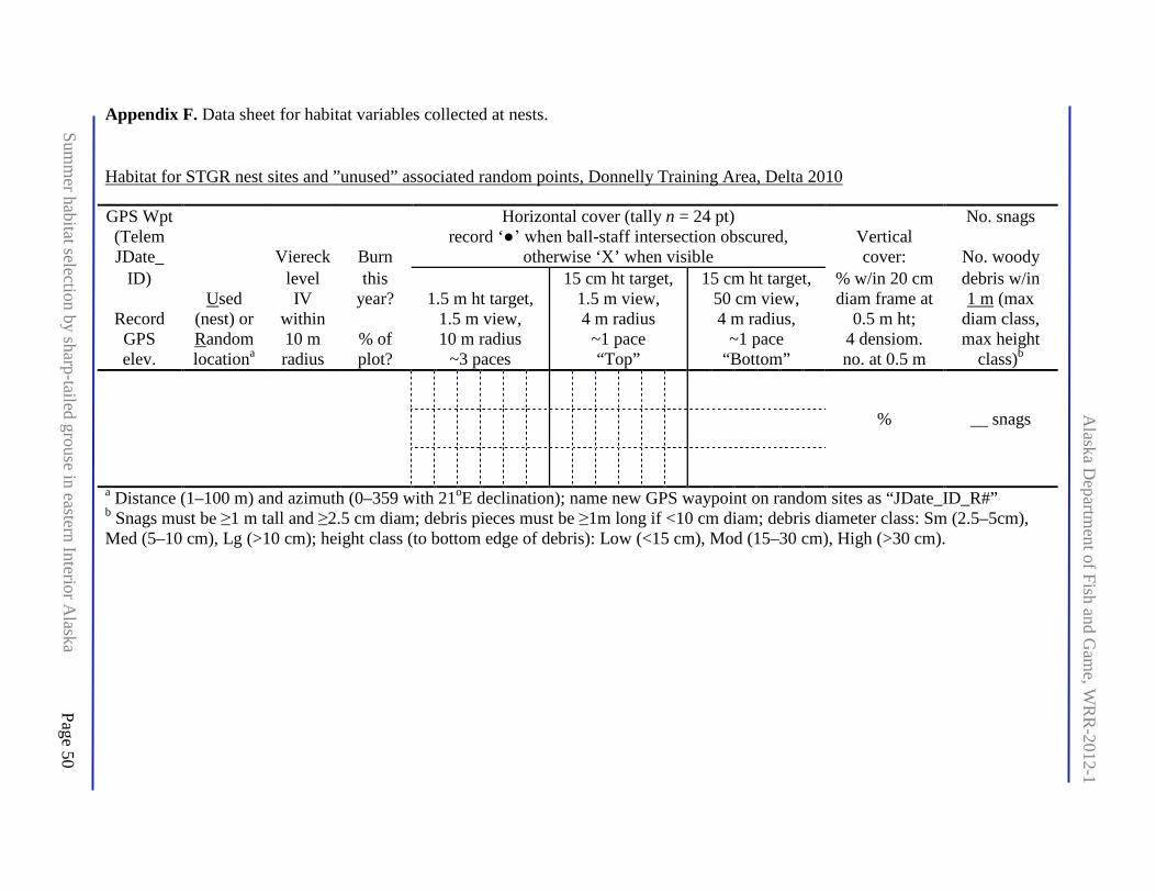
Alaska D
epartment of Fish and G
ame, W
RR
-2012-1
Summ
er habitat selection by sharp-tailed grouse in eastern Interior Alaska
Page 50
Appendix F. Data sheet for habitat variables collected at nests.
Habitat for STGR nest sites and ”unused” associated random points, Donnelly Training Area, Delta 2010
GPS Wpt (Telem JDate_ Viereck Burn
Horizontal cover (tally n = 24 pt) record ‘●’ when ball-staff intersection obscured,
otherwise ‘X’ when visible Vertical cover:
No. snags
No. woody ID)
Record
GPS elev.
Used (nest) or Random locationa
level IV
within 10 m radius
this year?
% of plot?
1.5 m ht target, 1.5 m view, 10 m radius
~3 paces
15 cm ht target, 1.5 m view, 4 m radius
~1 pace “Top”
15 cm ht target, 50 cm view, 4 m radius,
~1 pace “Bottom”
% w/in 20 cm diam frame at
0.5 m ht; 4 densiom. no. at 0.5 m
debris w/in 1 m (max
diam class, max height
class)b
%
__ snags
a Distance (1–100 m) and azimuth (0–359 with 21oE declination); name new GPS waypoint on random sites as “JDate_ID_R#” b Snags must be ≥1 m tall and ≥2.5 cm diam; debris pieces must be ≥1m long if <10 cm diam; debris diameter class: Sm (2.5–5cm), Med (5–10 cm), Lg (>10 cm); height class (to bottom edge of debris): Low (<15 cm), Mod (15–30 cm), High (>30 cm).

Alaska D
epartment of Fish and G
ame, W
RR
-2012-1
Summ
er habitat selection by sharp-tailed grouse in eastern Interior Alaska
Page 51
Appendix G. Survival parameters of sharp-tailed grouse in 2010, Donnelly Training Area, Alaska. Days of exposure to mortality risk are listed for alternative survival estimators (e.g., Heisey and Fuller 1985). Location of capture leks is shown in Figure 1.
Bird ID Sex Initial capture
lek Capture
date
Last known alive
(subseq. moved)
Last assumed alive (no
mort. signal)
Loss date to last loc. Mortality cause
Risk days 14 Apr–16 May
(displaying)
Risk days
17 May–23 Jun
(nesting)
Risk days 24 Jun–20 Sepa (brood rearing)
Risk days
24 Jun–last alive midpoint
573b F Keyhole S 7 May 20 Sep 21 Sep -- 10 38 89 89 573A F Sally 28 Apr 4 May Suspected raptor predation 7 -- -- -- 583a F Keyhole S 27 Apr 22 Sep 6 Oct -- 20 38 97 594 M Keyhole S 26 Apr 6 May Raptor predation 11 -- -- -- 614 M Keyhole N 27 Apr 30 Apr Unknown (partially scavenged) 4 -- -- -- 623 M TX Condo N 21 Apr 2 May Suspected raptor predation 12 -- -- -- 634 F Sally 27 Apr 6 May Unknown predation 10 -- -- -- 644 F Keyhole S 28 Apr 29 Apr Suspected goshawk predation at trap -- -- -- --
653 M TX Condo N 27 Apr 28 Sep 6 Oct -- 20 38 93 106 663 M Sally Satellite 24 Apr 1 Jul 6 Jul 12 Jul Unknown 23 38 13 13 673 M TX Condo S 23 Apr 28 Sep 6 Oct -- 24 38 39 106 684a F Sally 25 Apr 21 Sep 22 Sep -- 22 38 89 91 693 M Sally 17 May 28 Sep 4 Oct -- -- 38 92 104 704 M Sally 21 Apr 28 Sep 4 Oct -- 26 38 92 104 714 M Sally 14 Apr 23 Sep 4 Oct -- 33 38 95 105 724a F Keyhole S 27 Apr 7 Jun 12 Junc 12 Jun Suspected goshawk predation 20 26 -- -- 744 M Keyhole S 26 Apr 21 Sep 30 Sep -- 21 38 93 99 754 F Keyhole S 28 Apr 5 May Suspected raptor predation 8 -- -- -- 763 F Sally 27 Apr 4 May Raptor predation 8 -- -- -- 773 M Keyhole S 26 Apr 20 Sep 29 Sep -- 21 38 93 93 783 M Keyhole S 27 Apr 20 Sep 29 Sep -- 20 38 93 93
794 F Keyhole S 28 Apr 18 May Raptor predation 19 1 -- -- 803 M Sally Satellite 22 Apr 6 Oct -- -- 25 38 89 105 814a F Keyhole S 27 Apr 22 Sep 4 Oct -- 20 38 95 103 824 M Sally Satellite 22 Apr 28 Sep 4 Oct -- 25 38 92 104 833 M Sally 17 May 28 Sep 6 Oct -- -- 38 93 106 844 M Keyhole S 27 Apr 29 Sep 30 Sep -- 20 38 89 99 854 M Keyhole N 28 Apr 21 Sep 4 Oct -- 19 38 95 103 863a F Keyhole S 27 Apr 21 Sep 22 Sep -- 20 38 89 91
a Last date all remaining birds were confirmed alive at end of study. b Reproductive female. c Midpoint of unsuccessful search date (censor) or mortality signal and the prior location when confirmed alive.

Alaska Department of Fish and Game, WRR-2012-1
Summer habitat selection by sharp-tailed grouse in eastern Interior Alaska Page 52
Appendix H. Habitat selection ratios (proportion used divided by proportion available within 100% minimum convex polygon [MCP] home range) and standardized selection index by individual sharp-tailed grouse (female, male) during nesting and brood rearing on Donnelly Training Area, Alaska, May–September 2010.
Bird ID (MCP [ha])
Habitat type within home range
Available proportion
Used Selection ratioa
Selection indexb Prop. n
F573 (310)
Forest 0.8335 0.4286 12 0.51B 0.07 Grassland 0.0210 0.0714 2 3.40 0.46 Low scrub 0.0018 0.0000 0 0.00 0.00 Tall scrub 0.1437 0.5000 14 3.48A 0.47
F583c
(218) Forest 0.8367 0.4643 13 0.55B 0.03 Grassland 0.0150 0.1786 5 11.92A 0.68 Low scrub 0.0013 0.0000 0 0.00 0.00 Tall scrub 0.1470 0.7500 21 5.10A 0.29
F684c
(90) Forest 0.0006 0.0000 0 0.00 0.00 Grassland 0.5092 0.5357 15 1.05B 0.06 Low scrub 0.4727 0.4643 13 0.98B 0.05 Tall scrub 0.0175 0.2857 8 16.35A 0.89
F814c
(841) Forest 0.7412 0.8214 23 1.11 0.03 Grassland 0.0623 0.1786 5 2.87 0.07 Low scrub 0.0010 0.0357 1 35.62 0.86 Tall scrub 0.1955 0.3929 11 2.01 0.05
F863c
(377) Forest 0.9659 0.4286 12 0.44C 0.01 Grassland 0.0141 0.1429 4 10.13B 0.24 Low scrub 0.0013 0.0000 0 0.00 0.00 Tall scrub 0.0187 0.6071 17 32.47A 0.75
M653 (123)
Forest 0.0068 0.0000 0 0.00 0.00 Grassland 0.5169 0.4643 13 0.90 0.18 Low scrub 0.4471 0.1429 4 0.32 0.07 Tall scrub 0.0292 0.1071 3 3.67 0.75
M673 (337)
Forest 0.0130 0.0000 0 0.00 0.00 Grassland 0.4136 0.2143 6 0.52B 0.16 Low scrub 0.4122 0.1786 5 0.43B 0.14 Tall scrub 0.1612 0.3571 10 2.22A 0.70
M693 (42)
Forest 0.0000 0.0000 0 —d —d Grassland 0.9901 0.6071 17 0.61B 0.02 Low scrub 0.0028 0.0357 1 12.93A 0.45 Tall scrub 0.0072 0.1071 3 14.96A 0.52
M704 (471)
Forest 0.0142 0.0000 0 0.00 0.00 Grassland 0.4231 0.1429 4 0.34 0.13 Low scrub 0.3930 0.3214 9 0.82 0.31 Tall scrub 0.1697 0.2500 7 1.47 0.56

Alaska Department of Fish and Game, WRR-2012-1
Summer habitat selection by sharp-tailed grouse in eastern Interior Alaska Page 53
Bird ID (MCP [ha])
Habitat type within home range
Available proportion
Used Selection ratioa
Selection indexb Prop. n
M714 (68)
Forest 0.0003 0.0000 0 0.00AB 0.00 Grassland 0.9874 0.5714 16 0.58B 0.01 Low scrub 0.0027 0.0357 1 13.04AB 0.33 Tall scrub 0.0095 0.2500 7 26.19A 0.66
M744 (433)
Forest 0.8060 0.3214 9 0.40B 0.13 Grassland 0.0214 0.0000 0 0.00AB 0.003 Low scrub 0.0010 0.0000 0 0.00AB 0.003 Tall scrub 0.1716 0.4643 13 2.71A 0.873
M773 (236)
Forest 0.8261 0.5357 15 0.65 0.19 Grassland 0.0194 0.0357 1 1.84 0.54 Low scrub 0.0009 0.0000 0 0.00 0.00 Tall scrub 0.1536 0.1429 4 0.93 0.27
M803 (27)
Forest 0.0000 0.0000 0 —d —d Grassland 0.9961 0.8929 25 0.90 0.03 Low scrub 0.0028 0.0000 0 0.00 0.00 Tall scrub 0.0011 0.0357 1 32.06 0.97
M824 (61)
Forest 0.0003 0.0000 0 0.00 0.00 Grassland 0.9767 0.5714 16 0.59C 0.01 Low scrub 0.0041 0.1429 4 35.17A 0.81 Tall scrub 0.0189 0.1429 4 7.55B 0.17
M833 (119)
Forest 0.0005 0.0000 0 0.00AB 0.00 Grassland 0.5220 0.3929 11 0.75B 0.04 Low scrub 0.4628 0.2143 6 0.46B 0.02 Tall scrub 0.0147 0.2857 8 19.49A 0.94
M854 (668)
Forest 0.7868 0.3214 9 0.41B 0.04 Grassland 0.1719 0.0000 0 0.001AB 0.00 Low scrub 0.0008 0.0000 0 0.001AB 0.00 Tall scrub 0.0405 0.3929 11 9.69A 0.96
a Ratio is proportion used divided by proportion available. Different letters indicate significant differences (P <0.05, Bonferroni correction) in pairwise comparisons of mean selection indices among habitat types for each bird. Samples of <5 locations per habitat type made statistical inference unwarranted. b Indices are the standardized ratio where highest value indicates highest relative selection by an individual. c Female had brood. d Habitat type absent from home range.

Alaska Department of Fish and Game, WRR-2012-1
Summer habitat selection by sharp-tailed grouse in eastern Interior Alaska Page 54
Appendix I. Mean (median in parentheses) visual concealment (%) at 4 m or 10 m distance by lek, individual, and period (nesting or brood rearing) for sharp-tailed grouse, Donnelly Training Area, Alaska, June–September 2010. The Wilcoxon test compared paired samples of used and random sites with a Z-statistic (negative test score indicates concealment is greater at used sites than at random sites at the alpha probability indicated). Only birds for which minimum convex polygon range was estimated (larger sample size) were included. Concealment Lek ID Period n pairs Used Random Test P
At 15 cm above ground from 1.5 m height and 4 m distance
Keyhole (forest)
F573a Nest 7 52.3 (62.5) 60.7 (62.5) 1.18 0.24 Rear 20 59.8 (54.2) 62.5 (72.9) 0.36 0.72
F583 Nest 6 79.2 (83.3) 61.1 (64.6) −1.36 0.17 Rear 47 50.2 (45.8) 60.6 (62.5) 2.37 0.02
F814 Nest 8 73.4 (87.5) 69.3 (79.2) 0.07 0.94 Rear 46 47.7 (43.8) 49.6 (45.8) 0.80 0.43
F863 Nest 4 72.9 (79.2) 32.3 (27.1) −1.83 0.07 Rear 29 52.3 (50.0) 57.2 (54.2) 0.76 0.45
M744 Nest 5 47.5 (54.2) 45.0 (50.0) −0.41 0.69 Rear 14 42.9 (47.9) 42.6 (39.6) −0.03 0.97
M773 Nest 6 64.6 (62.5) 36.1 (41.7) −2.20 0.03 Rear 13 47.8 (45.8) 42.9 (45.8) −0.75 0.46
M854 Nest 6 34.7 (41.7) 34.7 (41.7) 0.94 0.35 Rear 11 30.3 (25.0) 29.5 (33.3) −0.13 0.89
At 15 cm above ground from 1.5 m height and 4 m distance
Sally (grassland)
F684 Nest 3 88.9 (87.5) 72.2 (79.2) −0.54 0.59 Rear 42 58.0 (58.3) 60.5 (66.7) 0.16 0.88
M653 Nest 5 91.7 (95.8) 85.8 (95.8) −0.78 0.47 Rear 11 71.2 (75.0) 63.6 (62.5) −0.71 0.48
M673 Nest 3 48.6 (45.8) 63.9 (79.2) 1.60 0.11 Rear 12 76.4 (87.5) 72.6 (87.5) −0.18 0.86
M693 Nest 3 68.1 (91.7) 63.9 (75.0) −0.45 0.66 Rear 11 61.7 (58.3) 35.2 (20.8) −1.89 0.06
M704 Nest 5 81.7 (83.3) 71.4 (70.8) −0.94 0.35 Rear 10 72.1 (70.8) 60.8 (64.6) −1.07 0.28
M714 Nest 6 72.2 (75.0) 64.6 (77.1) −0.53 0.60 Rear 13 69.2 (70.8) 54.2 (54.2) −2.18 0.03
M803 Nest 4 60.4 (62.5) 34.4 (33.3) −0.73 0.47 Rear 13 44.2 (45.8) 39.4 (33.3) −0.56 0.58
M824 Nest 6 48.6 (54.2) 47.9 (56.3) 0.14 0.89 Rear 12 54.5 (58.3) 53.1 (43.8) 0.16 0.88
M833 Nest 5 69.2 (75.0) 88.3 (91.7) 0.41 0.68 Rear 13 63.5 (79.2) 55.1 (66.7) −0.43 0.67
At 1.5 m above ground from 1.5 m height and 10 m distance
Keyhole (forest)
F573a Nest 7 38.1 (29.2) 29.2 (20.8) −1.46 0.14 Rear 20 35.4 (29.2) 29.2 (20.8) −1.29 0.20
F583 Nest 6 22.9 (20.8) 43.1 (39.6) 1.57 0.12 Rear 47 23.1 (16.7) 27.7 (20.8) 1.57 0.12
F814 Nest 8 12.5 (12.5) 18.2 (16.7) 0.67 0.02 Rear 46 41.3 (37.5) 43.8 (39.6) 0.23 0.82
F863 Nest 4 33.3 (35.4) 44.8 (41.7) 0 1.0 Rear 29 45.3 (45.8) 41.5 (37.5) −0.062 0.54
M744 Nest 5 61.7 (70.8) 40.8 (41.7) −1.48 0.14 Rear 14 47.6 (47.9) 51.5 (45.8) 0.18 0.86
M773 Nest 6 59.0 (62.5) 41.0 (45.8) −1.57 0.12 Rear 13 26.0 (16.7) 24.0 (16.7) 0.31 0.76
M854 Nest 6 41.0 (25.0) 45.1 (43.8) 0.73 0.46 Rear 11 39.4 (54.2) 39.8 (25.0) 0.31 0.76

Alaska Department of Fish and Game, WRR-2012-1
Summer habitat selection by sharp-tailed grouse in eastern Interior Alaska Page 55
Concealment Lek ID Period n pairs Used Random Test P At 1.5 m above ground from 1.5 m height and 10 m distance
Sally (grassland)
F684 Nest 3 8.3 (4.2) 9.7 (8.3) 0.48 0.66 Rear 42 34.3 (29.2) 35.6 (20.8) 0.34 0.74
M653 Nest 5 36.7 (12.5) 16.7 (0) −0.73 0.47 Rear 11 21.6 (0) 10.2 (0) −0.95 0.34
M673 Nest 3 4.2 (0) 0 (0) −1.0 0.32 Rear 12 26.4 (6.3) 26.4 (0) −0.34 0.74
M693 Nest 3 0 (0) 4.2 (0) 1.0 0.32 Rear 11 4.2 (0) 6.4 (0) −0.53 0.60
M704 Nest 5 17.5 (8.3) 7.5 (4.2) −0.73 0.47 Rear 10 35.0 (25.0) 19.2 (0) −1.78 0.08
M714 Nest 6 15.3 (0) 0.7 (0) −1.09 0.28 Rear 13 20.8 (0) 3.2 (0) −2.02 0.04
M803 Nest 4 6.3 (0) 1.0 (0) −1.0 0.32 Rear 13 18.6 (0) 0 (0) −1.83 0.07
M824 Nest 6 16.0 (0) 0.7 (0) −1.0 0.32 Rear 12 23.3 (0) 9.7 (0) −1.83 0.07
M833 Nest 5 43.3 (37.5) 20.8 (8.3) −0.94 0.35 Rear 13 25.6 (4.2) 9.3 (0) −1.66 0.10
a Nested but did not rear a brood.

Alaska Department of Fish and Game, WRR-2012-1
Summer habitat selection by sharp-tailed grouse in eastern Interior Alaska Page 56
Appendix J. Viereck Level IV proportions of the minimum convex polygons (MCPs) of telemetry locations of sharp-tailed grouse associated with 2 breeding leks (51.1 km2) within eastern Donnelly Training Area (DTA) during May–September 2010. Habitat type in leks was ranked by proportion of total area in the leks, and average size of habitat polygons in the lek MCPs is reported. The first 8 types composed 95% of the combined leks. This classification was not validated for accuracy.
Viereck type description Viereck Level IV
% Total area leks
Habitat type (Viereck I or
II) Avg. polygon in leks (ha)
Closed dwarf birch/willow/ericaceous 2C1Q 36.46 Low scrub 56.44 Open mat cushion/dryas/ericaceous/willow (hill top)
2D1A 27.09 Low scrub 69.18
Open alder/willow/shrub birch 2B2D 13.07 Tall scrub 24.74 Woodland aspen 1B3J 6.37 Forest 108.47 Open shrub birch-willow-ericaceous 2C2C 5.75 Low scrub 97.82 Closed alder/willow/shrub birch 2B1D 3.14 Tall scrub 6.41 Closed black spruce 1A1K 1.74 Forest 9.88 Wet sedge grass 3A2D 1.49 Grassland 19.03 Open aspen 1B2B 0.80 Forest 1.45 Closed alder 2B1B 0.64 Tall scrub 6.51 Closed black spruce and birch 1C1A 0.46 Forest 1.82 Closed moist sedge/grass (seasonally flooded) 3A2E 0.39 Grassland 2.19 Closed birch 1B1D 0.38 Forest 4.91 Water bodies <20 acres 8B2 0.38 N/A 1.29 Bare ground, roads, gravel pits, mines, quarries 7F3 0.31 N/A 0.99 Closed aspen/balsam poplar 1B1G 0.25 Forest 6.30 Closed white spruce 1A1J 0.20 Forest 1.45 Closed dry bluejoint/herb (hill top) 3A2B 0.19 Grassland 1.20 Closed black and white spruce-aspen 1C1D 0.19 Forest 3.16 Open black spruce 1A2F 0.16 Forest 2.75 Closed aspen 1B1E 0.15 Forest 0.74 Woodland black spruce 1A3D 0.12 Forest 0.91 Open balsam poplar 1B2C 0.11 Forest 1.90 Closed balsam poplar 1B1C 0.07 Forest 1.22 Open black spruce aspen 1C2B 0.04 Forest 0.65 Open white spruce 1A2E 0.03 Forest 0.31 Dry midgrass-herb-sedge 3A1B 0.01 Grassland 0.70 Rock 7B3 0.01 N/A 0.29 Closed black and white spruce 1A1L 0.01 Forest 0.38 Woodland black and white spruce-aspen 1C3G <0.01 Forest <0.01

Alaska Department of Fish and Game, WRR-2012-1
Summer habitat selection by sharp-tailed grouse in eastern Interior Alaska Page 57
Appendix K. Box plots showing median (middle vertical line in box) and interquartile range (IQR: 25th–75th percentiles as vertical box edges) for distance (m) moved between successive locations for female and male sharp-tailed grouse on Donnelly Training Area, Alaska, May–September 2010. Horizontal lines beyond box represent 1.5 times the IQR, with extreme values shown as an asterisk or circle. Non-normal distributions (Lilliefors test, P <0.05) are in bold.
F573 (n = 23 location pairs)
F583 (n = 29)
F684 (n = 26)
F814 (n = 30)
F863 (n = 26)
M653 (n = 16)
M673 (n = 17)
M693 (n = 18)
0 500 1000 1500 2000 2500DIST_M
0 500 1000 1500 2000DIST_M
0 500 1000 1500DIST_M
0 500 1000 1500 2000 2500DIST_M
0 1000 2000 3000DIST_M
0 100 200 300 400 500 600 700 800 900 1000
DIST_M
0 1000 2000 3000DIST_M
0 100 200 300 400 500 600 700 800DIST_M

Alaska Department of Fish and Game, WRR-2012-1
Summer habitat selection by sharp-tailed grouse in eastern Interior Alaska Page 58
M704 (n = 16)
M714 (n = 21)
M744 (n = 19)
M773 (n = 18)
M803 (n = 22)
M824 (n = 19)
M833 (n = 21)
M854 (n = 18)
0 1000 2000 3000 4000DIST_M
0 500 1000 1500 2000DIST_M
0 1000 2000 3000 4000 5000 6000DIST_M
0 500 1000 1500 2000 2500DIST_M
0 100 200 300 400 500 600 700DIST_M
0 100 200 300 400 500 600 700 800DIST_M
0 500 1000 1500 2000DIST_M
0 1000 2000 3000 4000DIST_M


©2010 ADF&G, photo by Tom Paragi. Sally lek study area for sharp-tailed grouse, Donnelly Training Area, Alaska.
©2010 ADF&G, photo by Tom Paragi. Keyhole study area for sharp-tailed grouse, Donnelly Training Area, Alaska.