Embed Size (px)
Citation preview

1
ANTHROPOGENIC HEAT IN THE CITY OF SÃO PAULO, BRAZIL
Mauricio Jonas Ferreira, Amauri Pereira de Oliveira and Jacyra Soares
Group of Micrometeorology, Department of Atmospheric Sciences
Institute of Astronomy, Geophysics and Atmospheric Sciences
University of São Paulo, São Paulo, Brazil
Sunday, August 01, 2010
Corresponding author Amauri P. de Oliveira Departamento de Ciências Atmosféricas – IAG/USP Rua do Matão, 1226 05508.090 – São Paulo, SP Brazil Tel. 55.11.30914701 Fax. 55.11.30914714 Email: [email protected]

2
Abstract The main goal of this work is to describe the anthropogenic energy flux (QF) in
the city of São Paulo, Brazil. The hourly, monthly and annual values of the anthropogenic
energy flux are estimated using the inventory method, and the contributions of vehicular,
stationary and human metabolism sources from 2004 to 2007 are considered. The vehicular
and stationary sources are evaluated using the primary consumption of energy based on
fossil fuel, bio fuel and electricity usage by the population. The diurnal evolution of the
anthropogenic energy flux shows three relative maxima, with the largest maxima occurring
early in the morning (∼19.9 Wm-2) and in the late afternoon (∼20.3 Wm-2). The relative
maximum that occurs around noontime (∼19.6 Wm-2) reflects the diurnal pattern of vehicle
traffic that seems to be specific to São Paulo. With respect to diurnal evolution, the energy
flux released by vehicular sources (QFV) contributes approximately 50% of the total
anthropogenic energy flux. Stationary sources (QFS) and human metabolism (QFM) represent
about 41% and 9% of the anthropogenic energy flux, respectively. For 2007, the monthly
values of QFV, QFS, QFM and QF are, respectively, 16.8 ± 0.25 MJ m-2 month-1, 14.3 ± 0.16
MJ m-2 month-1, 3.5 ± 0.03 MJ m-2 month-1 and 34.6 ± 0.41 MJ m-2 month-1. The seasonal
evolution monthly values of QFV, QFS, QFM and QF show a relative minimum during the
summer and winter vacations and a systematic and progressive increase associated with the
seasonal evolution of the economic activity in São Paulo. The annual evolution of QF
indicates that the city of São Paulo released 355.2 MJ m-2 year-1 in 2004 and 415.5 MJ m-2
year-1 in 2007 in association with an annual rate of increase of 19.6 MJ m-2 year-1 (from
2004 to 2006) and 30.5 MJ m-2 year-1 (from 2006 to 2007). The anthropogenic energy flux
corresponds to about 9% of the net radiation at the surface in the summer and 15% in the
winter. The amplitude of seasonal variation of the maximum hourly value of the diurnal
variation increases exponentially with latitude.
Key words: Anthropogenic energy flux, energy balance, net radiation, São Paulo,
urban climate.

3
List of symbols
A Urbanized area (m2)
aFuel Fraction of vehicles by fuel type
CElectr Monthly consumption of electricity by stationary sources (GWh month-1)
CFuel Monthly consumption of fuel by vehicular or stationary sources (m3 month-1)
EDPC Energy flux released from daily consumption of electricity by stationary
sources (MJ m-2 day-1)
EVFuel Energy released by vehicles per distance traveled and fuel type (J m-1)
EVT Total energy released from fuel combustion of vehicles per traveled distance
(J m-1)
f Hourly fraction of the daily consumption of electricity by stationary sources
FDPC Energy flux released from daily consumption of fuel by stationary sources
(MJ m-2 day-1)
FE Fuel economy (m l-1)
Ft Traffic fraction
g Fraction of fuel consumption by stationary sources
Lat Latitude (degree)
M Rate of metabolic production of energy per person (W)
n Number of persons or animals
nD Number of days in the month
NHCElectr Net heat released by the consumption of electricity by stationary sources (J
KWh-1)
4
NHCFuel Net heat released by fuel combustion per fuel type from vehicular or
stationary sources (J kg-1)
NWRP Number of residents (person)
pcDVD Mean traveled distance of vehicles per person per day (m person-1 day-1)
ρFuel Fuel density (kg m-3)
ρpop Population density (person m-2)
Q* Net radiation
QF Anthropogenic energy flux
MAXFQ
Maximum hourly value of the diurnal evolution of QF
∆QS Heat storage
QH Turbulent sensible heat
QLE Turbulent latent heat
∆QA Heat advection
QFM Anthropogenic energy flux released by human and animal metabolism
QFS Anthropogenic energy flux released by stationary sources
QFSE Anthropogenic energy flux released from the consumption of electricity by
stationary sources
QFSF Anthropogenic energy flux released from the consumption of fuel by
stationary sources.
QFV Anthropogenic energy flux released by vehicular sources
R2 Coefficient of determination
WP Number of nonresidents (person)

5
CET Municipal Company of Transportation
CETESB Environmental protection agency of the State of São Paulo
DETRAN Department of transportation of the State of São Paulo
IAG Institute of Astronomy, Geophysics and Atmospheric Sciences
IBGE Brazilian Institute of Geography and Statistics
LPG Liquefied Petroleum Gas
MRSP Metropolitan region of São Paulo City
ONSE National Operator of the Brazilian Electric System
SSE State of São Paulo Energy and Sanitation Agency
UHI Urban heat island
6
1 Introduction
In urban regions, the progressive substitution of natural surfaces by artificial materials and
the continuous release of gas and particulate matter in the atmosphere contribute to
environmental degradation and may change local patterns of weather and climate (Oke
1988; Arnfield 2003; Collier 2006; Mills 2007). One way of assessing the impact of urban
occupation is to evaluate the energy balance at the surface. In this study, the energy balance
is expressed as ASLEHF* QQQQQQ ∆+∆++=+ , where Q* is the net radiation flux, QF is
the anthropogenic energy flux, QH and QLE are the turbulent sensible and latent heats, ∆QS
is the heat storage and ∆QA is the heat advection in the urban canopy (Oke 1988).
The anthropogenic energy flux is composed of three parts, FMFSFVF QQQQ ++= , where
QFV, QFS and QFM indicate, respectively, the anthropogenic energy fluxes released by
vehicular sources (fuel combustion), stationary sources (electricity and fuel consumed by
houses, industrial and commercial activities and for public lighting) and metabolism (human
and animal).
There are basically two methods to estimate the anthropogenic energy flux: the method
of residues and the method of energy inventory. The method of residues consists of
estimating the anthropogenic energy flux in terms of the energy balance equation. In reality,
this method requires the evaluation four out of six components of the energy balance
equation at the surface. The energy inventory method is the most applied technique for
estimating the anthropogenic energy flux in urban areas (Grimmond 1992; Kłysik 1996;
Sailor and Lu 2004; Smith et al. 2009). This method requires information about the primary
energy consumption of vehicles, industries and commercial and residential dwellings. The
composition of the different forms of primary energy consumption between vehicular and
stationary sources of the anthropogenic energy flux and the energy contribution due to

7
human and animal metabolism vary according to city. In general, this information is
obtained from statistical reports about the energy use of a particular city or country. The
inventory method assumes that all primary energy usage is transformed into heat, which is
released to the urban canopy. The delay between primary energy usage and its restitution to
the system (urban canopy) as heat is assumed to be zero (Ichinose et al. 1999; Sailor and Lu
2004).
There are several ways to apply the energy inventory method (Grimmond 1992; Kłysik
1996; Sailor and Lu 2004). Sailor and Lu (2004) evaluated the contribution of vehicular
sources in terms of the population density, energy used per vehicle and daily distance
traveled by vehicle per person. Grimmond (1992) estimated the contribution of vehicular
sources directly from the number of vehicles, road type and length, source area and energy
usage per vehicle.
The objective of this work is to estimate the diurnal, seasonal and annual variations of
the anthropogenic energy flux of the city of São Paulo, Brazil, using the energy inventory
method. Here, the anthropogenic energy flux will be estimated based on the contributions of
vehicular and stationary sources and the production of energy by the metabolism of the
city’s human population as proposed by Sailor and Lu (2004). This investigation is based on
statistical information available from federal and state agencies concerning the primary
energy consumption (fossil fuel, bio fuel and electricity) of the population from 2004 to
2007.
2 The city of São Paulo
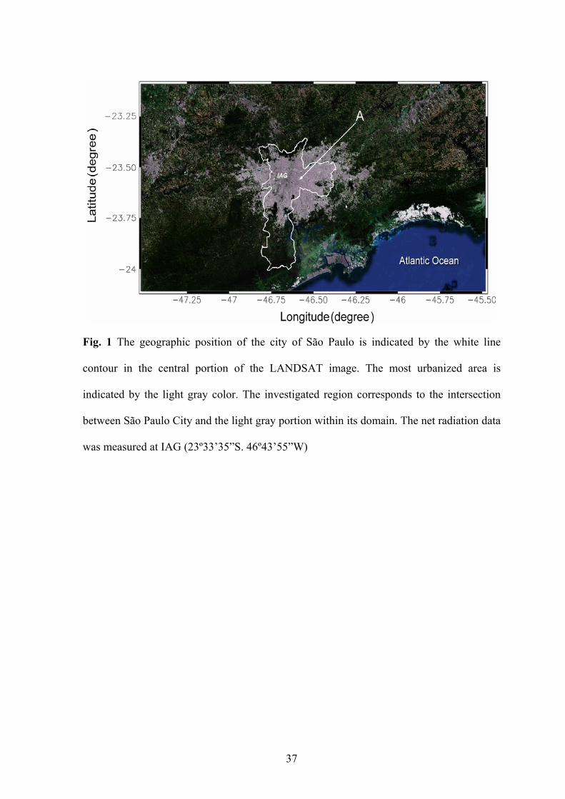
The city of São Paulo (23°33'1"S, 46°38'2"W) is located about 60 km from the Atlantic
Ocean and is approximately 700 m above mean sea level, as indicated the white line contour
in Fig. 1. The city contains the largest industrial park in South America (Codato et al. 2008).
8
This study will focus the most urbanized area of São Paulo, which covers an effective
area of 854 km2. The city’s 2007 population was 10,886,518, and it had 5,989,234 active
vehicles (CETESB 2008; DETRAN 2008; IBGE 2008). The study region corresponds to the
grey area within the city of São Paulo, as displayed in the satellite picture of Fig. 1.
According to Oliveira et al. (2002), the climate of São Paulo is typical of the subtropical
regions of Brazil, being characterized by a dry winter from June to August, and a wet
summer from December to February. The smallest daily values of temperature and relative
humidity occur in July and August (16°C and 74% respectively), and the lowest monthly
accumulated precipitation occurs in August (30 mm). The largest daily value of temperature
and monthly accumulated precipitation occurs in February (22.5°C and 255 mm), while the
maximum relative humidity (80%) is observed in two periods: December-January and
March-April.
Hereafter, February and August will be used to characterize the climate conditions
during summer and winter, respectively, in São Paulo. These months were chosen because
they are more representative of the summer-winter contrast in terms of precipitation, as
indicated in the climate description above.
3 Methodology
This work uses the energy inventory method to estimate the anthropogenic energy flux and
its temporal variations based on hourly monthly, monthly and annual values of electric
energy consumption and monthly and annual values of all fuel sold in the city of São Paulo
between 2004 and 2007.
The energy inventory method used here consists of summing up the following:
• The energy fluxes released by all moving vehicles in the city of São Paulo
considering the diurnal evolution of the number of vehicles in movement, the mean

9
distance traveled, the fuel consumed in distance traveled and the energy released by
fuel combustion (gasoline, hydrous alcohol and diesel oil) are used to estimate the
hourly annual values of the anthropogenic energy fluxes released by vehicular
sources.
• The energy released from the consumption of electricity and fuel (natural gas,
liquefied petroleum gas and fuel oil) by stationary sources (residential, industrial and
commercial activities and for public lighting) in São Paulo are used to estimate the
hourly monthly values of the anthropogenic energy flux released by stationary
sources.
• The energy flux released by the population’s metabolism is used to estimate hourly
annual values of the anthropogenic energy flux released by metabolic activity in the
city of São Paulo.
Alternatively, the energy fluxes released by the fleet of vehicles in movement in São
Paulo considering only the monthly consumption of fuel (gasoline, alcohol and diesel oil)
sold in the city is also used to estimate the monthly and annual values of the anthropogenic
energy flux released by vehicular sources. Most of the methodology used to estimate the
diurnal, seasonal and annual variations of QF, described hereafter, is based on Sailor and Lu
(2004).
3.1 Anthropogenic energy flux released by vehicular sources (QFV)
The diurnal evolution of QFV can be evaluated using the expression:
popTtFV EVFpcDVDQ ρ= (1)

10
Where pcDVD is the mean distance traveled by vehicles per person per day, Ft is the
traffic fraction, EVT is the total energy released from the fuel combustion of vehicles per
traveled distance and ρpop is the population density.
To estimate EVT representing the entire fleet of vehicles in a given city, it is necessary to
account for the energy released by vehicles per distance traveled by type of fuel combustion
(EVFuel) while considering the fraction of vehicles by type of fuel (aFuel), as indicated below:
∑=Fuel
FuelFuelT EVaEV (2)
Where EVFuel is estimated by:
FENHC
EV FuelFuelFuel
ρ= (3)
Where NHCFuel is the net heat released by the combustion of fuel, ρFuel is the fuel density
and FE is the fuel economy.
In general, the population of large conurbations shows a significant diurnal oscillation
caused by population movements from the border cities toward the core city. According to
Fulton (1984), the diurnal evolution of population density (ρpop) can be estimated for a
given city in terms of:
AWPNWRP
pop+
=ρ (4)
Where NWRP is the number of residents, WP is the number of nonresidents, namely,
those living outside the city that work or study in the city, and A is the urbanized area of the
city.
There are two different ways to obtain the monthly values of QFV (both methods will be
used here). One way is to use the integral of the diurnal evolution of QFV, given by

11
expression (1), multiplied by the number of days in each month (nD). The other way is by
using the following expression:
A
CNHCQ Fuel
FuelFuelFuel
FV
∑=
ρ
(5)
Where, CFuel is the monthly consumption of fuel by vehicular sources.
The annual values of QFV are estimated by adding all twelve monthly values in the year.
3.2 Stationary sources of anthropogenic energy flux (QFS)
The QFS is estimated using the consumption of electricity and other sources of energy
produced by the fuel combustion of natural gas, liquefied petroleum gas (LPG) and fuel oil.
This estimation can be expressed as:
FSFESFSF QQQ += (6)
Where, QFSE and QFSF are the anthropogenic energy flux released from the consumption
of electricity and fuel by stationary sources, respectively. These sources of energy are from
houses and buildings used for residential, commercial and industrial activities. Public
lighting in the urban region is also included.
The diurnal evolution of QFSE can be evaluated using the expression:
fEQ DPCFSE = (7)
Where, EDPC is the energy flux released from the daily consumption of electricity by
stationary sources and f is the hourly fraction of the daily consumption of electricity by
stationary sources.
12
The energy flux released by the daily consumption of electricity by stationary sources
(EDPC) can be estimated using:
AnCNHCE
D
ElectrElectrDPC = (8)
Where NHCElectr is the net heat released by the consumption of electricity by stationary
sources, CElectr is the monthly consumption of electricity by stationary sources and nD is the
number of days in the month.
The monthly values of QFSE can be estimated by integrating the diurnal evolution of
QFSE, given by expression (7), multiplied by the number of days. Numerically, the monthly
values of QFSE are equal to EDPC, given by expression (8), because the daily consumption of
electricity is constant, and the integral of f during a period of 24 hours is equal to 1.
By analogy with electricity, the diurnal evolution of QFSE can be estimated from the
energy flux released by the daily consumption of fuel by stationary sources:
gFQ DPCFSF = (9)
Where FDPC is the energy flux released from the daily consumption of fuel by stationary
sources, and g is the hourly fraction of the daily consumption of fuel by stationary sources.
Correspondently, the energy flux released from the daily consumption of each type of
fuel by stationary sources (FDPC) can be estimated using:
An
CNHCF
D
FuelFuelFuelFuel
DPC
∑=
ρ
(10)
Where NHCFuel is the net heat released by the consumption of fuel by stationary sources,
and CFuel is the monthly consumption of fuel by stationary sources.
13
Similarly, the monthly values of QFSF can be estimated by integrating the diurnal
evolution of QFSF given by expression (9) multiplied by the number of days in the month.
Numerically they are equal to FDPC given by expression (10) because the daily consumption
of fuel by stationary sources is constant, and the integral of g during a period of 24 hours is
equal to 1.
3.3 Human metabolism (QFM)
The diurnal evolution of QFM is estimated by:
popFM MQ ρ= (11)
Where, M is the rate of metabolic production of energy per person (Oke 1988;
Grimmond 1992; Sailor and Lu 2004).
The monthly values of QFM are estimated by the integral of diurnal evolution given by
expression (11) multiplied by the number of days in the month. The annual values of QFM
are estimated by adding all twelve monthly values in the year.
4 Diurnal variation of QF in the city of São Paulo
As indicated in the section above, to estimate the diurnal variation of QF is necessary to
evaluate the mean distance traveled by vehicles (pcDVD), traffic fraction (Ft), total energy
released by vehicles per distance traveled by type of fuel combustion (EVT), diurnal
evolution of population density (ρpop), hourly fraction of the daily consumption of
electricity (f) and fuel (g) by stationary sources in the city of São Paulo
According to Lents et al. (2004), pcDVD in São Paulo in 2004 was 17,000 km.
Considering that this mean distance traveled does not change much from one year to
another, in 2007 the mean distance traveled by vehicles per day was 46.6 km, and the mean

14
distance traveled by vehicles per person per day was 13,588 m person-1 day-1. A similar
extrapolation in time was calculated by Sailor and Lu (2004). In the pcDVD estimate for
São Paulo, the number of vehicles is set to 3,174,294, and the population is set to
10,886,518 inhabitants, both values corresponding to 2007. It should be emphasized that the
fleet of vehicles (3,174,294) in movement daily in São Paulo corresponds to 53% of the
total number of registered vehicles in São Paulo during 2007 (5,989,234). This fraction
(53%) is based on CET estimates (Roson 2008).
The traffic fraction Ft is estimated by considering that the number of vehicles in
movement in the main streets is representative of the traffic in São Paulo at each hour of the
day. Fig. 2 indicates the diurnal evolution of Ft based on the estimates of Lents et al. (2004)
for São Paulo in 2004. Aiming to inventory CO2 emissions, Lents et al. (2004) counted the
number of vehicles in movement in the most representative regions of São Paulo. In this
work, it is assumed that the Ft, observed by Lents et al. (2004) is valid for 2007. An
equivalent extrapolation in time was also done by Sailor and Lu (2004) for American cities.
The Ft, based on the observations carried out in 2004 (Fig. 2) matches the estimates
provided by the Municipal Company of Transportation of São Paulo City in 2007 (Roson
2008). The later estimates were based on observations carried out in 15 major avenues of
São Paulo during the rush hours (07:00 LT to 10:00 LT and 17:00 LT to 20:00 LT) in 2007.
As a reference, the traffic fraction in the USA, based on observations performed in 99 cities
over 19 states by Hallenbeck et al. (1997), is also indicated in Fig. 2. The Ft of the
American cities shows a behavior similar to that observed in São Paulo.
Table 1 indicates the values of NHCFuel, ρFuel and FE used to evaluate EVT in São Paulo.
The mean fuel economy corresponds to the mean values of fuel consumption of vehicles
that use gasoline, alcohol and diesel oil. The values in Table 1 are consistent with those
used to estimate the QF in other cities (Pirgeon et al. 2007). The contribution of motorcycles

15
is particularly relevant because São Paulo has a fleet of 349,256 motorcycles in movement
daily, corresponding to 53% of the 658,953 motorcycles registered up to 2007.
The only information available concerning the number of people visiting São Paulo daily
is based on the demographic data of the 2000 census analysis carried out by Aranha (2005)
and Ântico (2005). According to these authors, the city of São Paulo is the main destination
of the surrounding 38 cities, receiving between 590,000 and 612,000 people daily from
outside areas. Therefore, it will be assumed here that an average of 601,000 people visited
the city daily in 2000. To assess the daily population movement for 2004, 2005, 2006 and
2007, it was considered that the daily population displacement from the surrounding areas
increased according to the expected population growth, which was 2.24% between 2000 and
2004, 2.8% between 2000 and 2005, 3.36% between 2000 and 2006 and 4% between 2000
and 2007. Thus, the diurnal evolution of ρpop in 2007 is 0.0127 person m-2 at night (before
05:00 LT and after 19:00 LT) and 0.0135 person m-2 during the day (between 07:00 LT and
17:00 LT). The population densities during the night-to-day and day-to-night transition
periods are set to 0.0131 person m-2. These values were obtained by considering NWRP
equals 10,886,518 (IBGE, 2008), WP equals 625,000 people and the urbanized area A
equals 854 km2 in expression (4).
The hourly values of f was estimated using the diurnal evolution of the monthly average
values of electricity consumption in the State of São Paulo (ONSE, 2008). A similar method
was used by Sailor and Lu (2004) to estimate the hourly fraction of energy consumed daily
in several cities in the USA. The diurnal evolution of f in the city of São Paulo is indicated
in Fig. 4 for the summer and winter of 2007. For comparison, the hourly fraction of
electricity consumption for the USA cities proposed by Sailor and Lu (2004). Curiously, the
pattern of consumption of electricity in the State of São Paulo is similar the pattern of
consumption in the USA.

16
The hourly values of g were not available for 2007. Therefore, in the expression (9) the
hourly fraction is obtained by assuming that the daily consumption is evenly distributed
over the entire 24-hour period of 24. Thus, g is set to 0.0417 for the city of São Paulo.
4.1 Diurnal evolution of QF
Considering expressions (1)-(4), the diurnal evolution of the anthropogenic energy flux
released by vehicular sources is evaluated for 2007. In this case, neither the diurnal
evolution of the population density nor pcDVD change during the months within a year.
This value varies only from one year to another, which is why the diurnal evolution of QFV
is based on the hourly annual values of these variables.
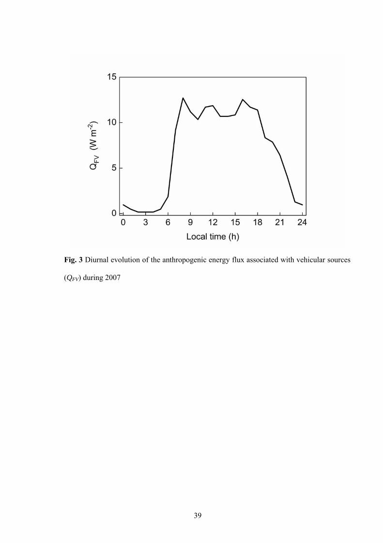
The diurnal evolution of QFV in São Paulo shows three peaks (Fig. 3). Two of these
peaks correspond to the hours when the traffic is most intense (early morning and evening).
The local maximum between 10:00 LT and 12:00 LT corresponds to the release period for
restricted vehicles based on license plate number. During the driving restriction hours
(07:00-10:00 LT and 17:00-20:00 LT), 20% of the vehicles are not allowed in the central
portions of São Paulo. The local maximum between 10:00 LT and 12:00 LT is a peculiarity
of São Paulo that is due to this traffic restriction.
The diurnal variation of QFS for the summer (February) and winter (August) of 2007 is
indicated Fig. 5. In the summer of 2007, QFS varied from 4.51 Wm-2 at 04:00 LT to 6.01
Wm-2 at 16:00 LT (Fig. 5a). In the winter, QFS varied from 4.77 Wm-2 at 03:00 LT to 6.81
Wm-2 at 19:00 LT (Fig. 5b). Comparatively, the amplitude of the diurnal cycle in summer
(1.50 Wm-2) is slightly smaller than that observed in the winter (2.04 Wm-2, Fig. 5b).
In the case of QFM the diurnal evolution was estimated using, in expression (11), the
population density estimates for 2007 and an energy release from metabolic activity of 75
W for the period of less activity (from 23:00 LT to 05:00 LT) and 115 W for the period of

17
greater activity (from 07:00 to 21:00 LT), as proposed by Oke (1988). In the transition
periods (05:00 LT to 07:00 LT and 21:00 LT to 23:00 LT), the rate of metabolic energy
released was estimated by a linear interpolation between the values of lesser and great
activity and vice versa. The energy released by animal metabolism was not considered
because there is no information about the number and type of animals in the city of São
Paulo.
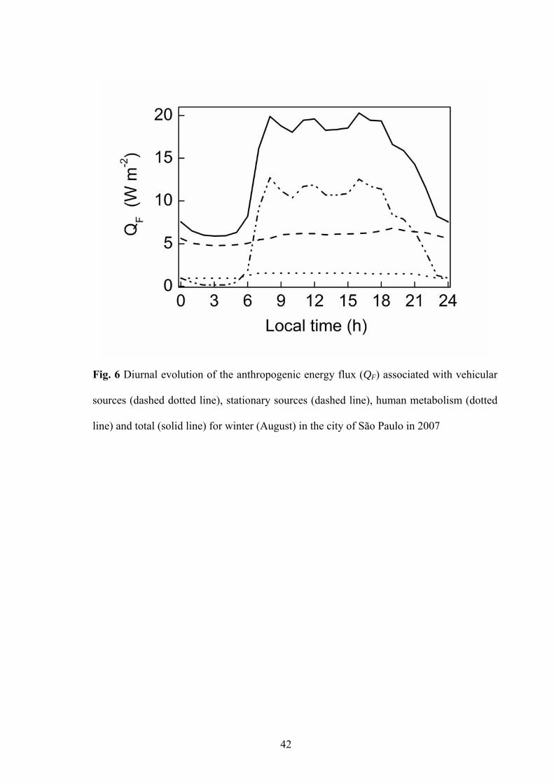
The diurnal cicle of QFV, QFS , QFM and QF for August are indicated in Fig. 6.
Comparatively to the diurnal evolution for February QF for August is not significantly
different. The relative difference is equal to 2% and it is due to the variation in the QFS. The
small seasonal variation observed in the diurnal evolution of QF (Fig. 6), with the winter
(August) values systematically larger than the summer (February) values, corroborates the
belief that even for a subtropical city like São Paulo, one should expect larger values of QF
in winter than in summer. However, as discussed above, this comparison is somehow
misleading because the results shown in Fig. 6 reflect only the seasonal variation of QFS. To
avoid this problem, the analysis of the seasonal variation of QF and its components will be
carried out in the next sections using monthly values exclusively. The analysis in this
section will focus only on the contributions of vehicular, stationary and human metabolic
sources in the diurnal evolution of QF.
The QF shows a diurnal evolution with three relative maxima, with the largest occurring
early in the morning (∼19.9 Wm-2) and in the late afternoon (∼20.3 Wm-2). The relative
maximum, which occurs around noontime (∼19.6 Wm-2), reflects the diurnal pattern of
vehicle traffic that seems to be specific to São Paulo (Fig. 6).
Considering the entire daytime period, the integral of diurnal evolution of the energy flux
released by vehicular sources contributes approximately 50% of the total anthropogenic

18
energy flux. The stationary sources and human metabolism represent about 41% and 9% of
the anthropogenic energy flux, respectively.
5 Seasonal variation of QF in the city of São Paulo
The seasonal evolution of QF was characterized using monthly values of the anthropogenic
energy flux released by vehicular, stationary and metabolic sources in São Paulo City, as
indicated in Fig. 7 (for 2007 only) and Fig. 8 (2004 to 2007).
In 2007, the mean monthly values of QFV, QFS, QFM and QF were, respectively, 16.8 ±
0.25 MJ m-2 month-1, 14.3 ± 0.16 MJ m-2 month-1, 3.5 ± 0.03 MJ m-2 month-1 and 34.6 ±
0.41 MJ m-2 month-1.
The vehicular source is the dominant factor during summer and winter (Fig. 7a).
Approximately 51% of QF was due to the energy released by 3.2 million vehicles traveling
daily in São Paulo (Lents et al. 2004; Roson 2008).
The energy released by the stationary sources is responsible for approximately 41% of
the QF (Fig. 7a). This figure remains relatively constant throughout the year, which may
indicate that these sources do not use electricity or fuel for heating during winter or for
cooling during summer. Indeed, São Paulo is located in a region of subtropical climate
where most of the residences and buildings do not require heating during winter.
The energy released by metabolic activities in São Paulo contributes 8% of QF (Fig. 7a).
In most cases described in the literature, the energy released by metabolic activities
represents 2-3% of QF (Oke 1988; Grimmond 1992; Sailor and Lu 2004). An exception is
Tokyo, where the contribution from metabolic sources is 5-10% (Ichinose et al. 1999). In
cities located in countries that have lower per capita energy consumption, the QFM
contribution to QF can be greater than 5% (Sailor and Lu 2004). São Paulo occupies an
upper range of QFM contribution to QF because of its large number of inhabitants (more than

19
11 million) and the low per capita energy consumption of its population (Sailor and Lu
2004).
The apparent lack of correlation between the time variation of QF and the seasonal
evolution of São Paulo’s climate is better visualized by the relative deviation from the
annual mean of the vehicular (white column), stationary (gray column) and metabolic (light
gray column) sources and QF (continuous line) displayed in Fig. 7b for 2007. In general, QF
and its major components, QFV and QFS, show a variation smaller than ±10%. During the
vacation periods, which occur at the beginning (January and February) and middle of the
year (July), the relative deviations of QF and QFV are negative. The largest negative
deviation, approximately -10%, is observed during the summer vacation period. After the
summer vacation in January and before the winter vacation in July, the relative deviations
of QFV and QFS oscillate around zero, while QF goes through a minimum negative in May
and increases progressively, becoming positive due to the augmentation in QFV. During the
second semester, the relative deviation of QF becomes positive. These patterns are basically
associated with the increase in economic activity that begins after the summer vacation,
showing a maximum in November. Therefore, the time evolution of QF in São Paulo is not
related to the seasonal evolution of the local climate but, rather, closely follows the city’s
economic activity.
The patterns found for 2007 are also observed in the period from 2004 to 2007 (Fig. 8).
In general QF, QFV and QFS increase after the summer vacation period at the beginning of the
year and decrease slightly during the winter vacation period (Fig. 8).
One important result observed in Fig. 8 is the progressive annual increase in the
amplitude of the monthly values of QF, QFV and QFS between 2004 and 2007. This effect
will be explored further in the following sections.

20
5.1 Seasonal variation of QF in terms of net radiation
Figure 9 shows a comparison between the seasonal evolution of net radiation and QF
observed in São Paulo. The net radiation was observed at the IAG site (Fig. 1) from 2004 to
2007 using a net radiometer from Kipp-Zonen (Ferreira et al. 2007).
The total input of energy in the urban canopy (Q* + QF) is 365.8 MJ m-2 month-1 in
February (summer) and 249.3 MJ m-2 month-1 in August (winter), and QF contributes about
29.4 MJ m-2 month-1 in February and 33.0 MJ m-2 month-1 in August. The average monthly
values of QF correspond to approximately 9% of the monthly values of the net radiation at
the surface during summer and 15% during winter. Annually, the anthropogenic energy flux
represents nearly 11% of the net radiation observed in São Paulo.
5.2. Seasonal variation of QF in terms of latitude
The intensity of the seasonal variation of QF is strongly correlated with climate. In general,
cities in the middle and high latitudes use more energy during winter for heating and
lighting, while in cities located in the low latitudes, like São Paulo, the energy used for
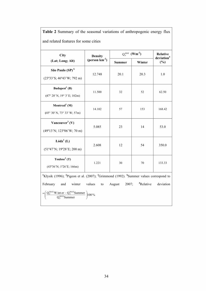
heating and lighting is small or even negligible. Table 2 shows the anthropogenic energy
flux (daily maximum) during the summer and winter months in São Paulo compared to
several cities located in the middle and high latitudes (Grimmond 1992; Kłysik 1996; Sailor
and Hart 2006; Pigeon et al. 2007).
In São Paulo the QF shows no significant seasonal variations. The relative deviation,
estimated as the ratio of winter-summer difference for São Paulo is 1.0 % (Table 2). In high
latitude cities the relative deviation varies from 53% (Vancouver) to 350% (Lodz).
The dependence of QF on climate can be better visualized in Fig. 10. There, the points in
the scatter plot with small scattering indicate the relationship between the seasonal
variations of QF and the latitude. These points correspond to cities in Table 2 and in the

21
Table 1 of Sailor and Hart (2006). The interpolated curve was obtained with a coefficient of
determination (R2) equal to 0.89, using 62 points (indicated by solid circle in Fig. 10. The 4
cities displayed by solid star correspond to Budapest, Portland, Seattle and Vancouver was
not included in the interpolation. Based on the available information there is no apparent
reason for the discrepant behavior of these 4 cities. However, if 62 out of 66 cities follow
the interpolate curve with R2 = 0.89, it can be concluded that the seasonal variation of QF
increases exponentially with latitude, as indicated in Fig. 10.
6 Inter-annual variations of QF in São Paulo
The time variation of the annual values of QFV, QFS and QF considering the annual
consumption of fuel and electricity by vehicular and stationary sources, as described in
Tables 3 and 4, are indicated in Fig. 11 for 2004-2007.
The annual values of QFV (Fig. 11a) indicate that the energy released by vehicular
sources associated with the combustion of gasoline, diesel oil, hydrous alcohol and
anhydrous alcohol increases at an annual rate of 1.5 MJ m-2 year-1, 1.0 MJ m-2 year-1, 5.2 MJ
m-2 year-1 and 1.3 MJ m-2 year-1, respectively. The total energy released from the
combustion of fuel increases at an annual rate of 8.1 MJ m-2 year-1. Because the number of
cars during this period remains relatively constant, the only significant variation that affects
the annual evolution of QFV components individually is the increase in the fraction of
vehicles fueled by hydrous alcohol, which varied from 15.4% in 2004 to 21.5% in 2007
(Table 3). Given the fact that diesel oil vehicles remain constant and the increase in alcohol
vehicles is followed by a decrease in the fraction of vehicles fueled by gasoline, the annual
rate of increase in QFV seems to be due to changes in the number of cars fueled by alcohol.
It should be emphasized that the numbers of vehicles in Table 3 correspond to the vehicles
registered in the city of São Paulo up to December 31 in each year.

22
Comparatively, the energy released annually from the consumption of electricity and fuel
(natural gas, LPG and fuel oil) by the stationary sources is indicated in Fig. 11b. This figure
shows that the annual evolution of energy released from the consumption of electricity,
natural gas, LPG and fuel oil by stationary sources has grown annually at a rate of 4.3 MJ
m-2 year-1 and 2.8 MJ m-2 year-1, respectively. The energy released from the consumption of
LPG has slightly increased during this period, whereas the energy released from the
combustion of oil decreased annually by about 0.5 MJ m-2 year-1.
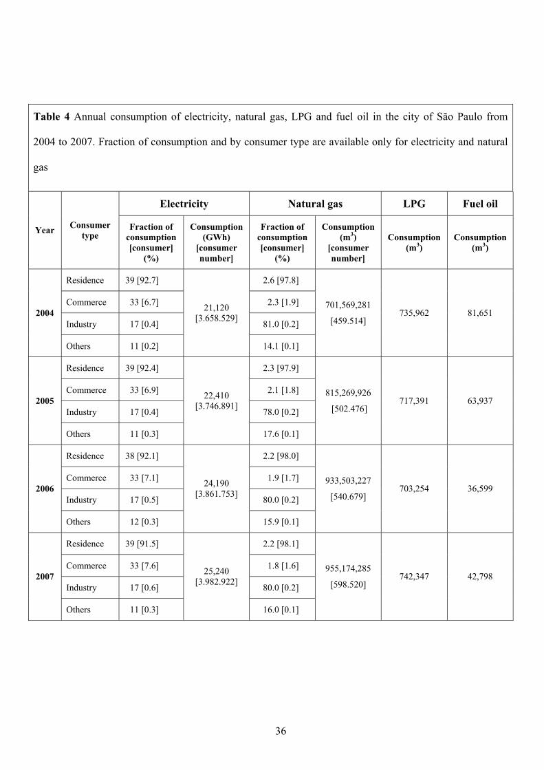
Table 4 shows the annual consumption of electricity in São Paulo from 2004 to 2007 and
the fraction of electricity usage per consumer type (residence, commerce, industry and
others). As can be seen in Table 4, almost 40% of the electricity consumption in São Paulo
is used in residences, about 30% is used in commerce and less than 20% is consumed by the
industrial sector. The progressive increase in the consumption of electricity from 2004 to
2007 reflects the growth of the industrial sector and other economic sectors in Brazil (Silva
and Guerra 2009). Moreover, the annual values in Table 4 indicate that the industrial sector
is responsible for the major consumption of natural gas (about 80% of total consumption).
The residential and commercial sector accounted for only 2.5% of total consumption in
2007 (Table 4).
The time variation of QF (Fig. 9c) indicates an increase at an annual rate of 19.6 MJ m-2
year-1 from 2004 to 2006 and 30.5 MJ m-2 year-1 in 2007. The city of São Paulo released
355.2 MJ m-2 year-1 in 2004 and 415.5 MJ m-2 year-1 in 2007. These variations reflect the
annual increases observed in QFV (Fig. 11a) and QFS (Fig. 11b). Annually, the contributions
of QFV, QFS and QFM to the anthropogenic energy flux were 47.5%, 42.0% and 10.5%,
respectively. These fractions of annual values of QF are consistent with those based on
diurnal and seasonal evolution in the previous sections.
7 Conclusions
23
The main objective of this work was to describe the anthropogenic energy flux of São Paulo
using the energy inventory method.
Based on the results described in the previous sections, one can conclude the following:
• The diurnal evolution of QF shows three relative maxima, with the largest occurring
early in the morning (∼19.9 Wm-2) and in the late afternoon (∼20.3 Wm-2). The
smallest relative maximum occurs around noontime (∼19.6 Wm-2) for 2007.
• The energy released by vehicular sources is dominant term, contributing 50% (49.0%
monthly and 47.5% annually) of the total anthropogenic energy flux.
• The stationary sources and human metabolism contribute approximately 41% (41%
monthly and 42% annually) and 9% of the anthropogenic energy flux, respectively
(10% monthly and 10.5% annually).
• There is no significant seasonal variation for the stationary sources of anthropogenic
energy flux, indicating the city of São Paulo does not require a significant amount of
energy for heating or lighting in the winter as do cities in higher latitudes or higher
altitudes (Sailor and Lu, 2004).
• The anthropogenic energy flux corresponds to 9% of the net radiation in the summer
and about 15% in the winter. The annual average values of the anthropogenic energy
flux are near 11% of the net radiation from 2004 to 2007.
In most of the work available in the literature, the fraction of vehicular sources
contributing to the total anthropogenic energy flux varies between 47% and 62%. In São
Paulo, the vehicular fraction is 52%. This large contribution reflects:
a) the large number of vehicles circulating daily, at around 3.2 million or half of the
total existing fleet; and
b) the high average distance traveled by these vehicles, at 46.6 km per day.

24
The number of cars traveling daily in the city of São Paulo is greater than most cities
where the anthropogenic energy flux has been evaluated (Table 2). The large fleet in São
Paulo is the direct consequence of an incipient public transportation system that is present in
most third world cities.
One important result from this work is that the diurnal evolution of both vehicle traffic
(traffic fraction) and electricity consumption were estimated objectively for the city of São
Paulo, and they happened to similar to the diurnal evolution found in cities in the USA.
Another important conclusion is that the seasonal variation of the anthropogenic energy flux
varies exponentially with latitude. An empirical expression represented by an exponential
growth was fitted with a coefficient of determination of 0.89, considering 62 of 66 cities.
Another important point brought up by this work is that QF, according to the estimates
carried out here, is increasing at an annual rate of 19.6 MJ m-2 year-1 (∼5%). This indicates
that QF may increase by about 50% in 10 years. This increase may intensify the effects
associated with the anthropogenic release of energy on the urban climate of São Paulo,
especially in the urban heat island.
This study is based on the hypothesis that all of the energy released by vehicular,
stationary and metabolic sources is evenly distributed over the urbanized area of São Paulo
(854 km2). In comparison to other large cities (Table 2), the relatively small values of the
anthropogenic energy flux in São Paulo (∼20 W m-2) may be a consequence of this
hypothesis. One would expect larger QF values if small and highly urbanized areas were
considered isolated (Kłysik 1996; Ichinose et al. 1999). In this case, a larger QF would be
confined to small portions of São Paulo and would be a major source of energy for the
spatial variations in its urban heat island (UHI). It is known that in some areas of São Paulo,
the UHI may reach as much as 12oC (Monteiro 1976). The next step will be to investigate
the spatial variability of QF in São Paulo.

25
Acknowledgments The authors acknowledge the financial support provided by CAPES and
CNPq (476.807/2007-7). We offer thanks to Antonio Carlos Roson, the CET Chief
Engineer, for providing data about vehicle traffic in São Paulo. We also thank João Ricardo
Neves for his valuable assistance.
26
References
Ântico C (2005) Displacements commuters in the metropolitan region of São Paulo.
Available in Portuguese. São Paulo in Perspective 19: 110-120. doi: 10.1590/S0102-
88392005000 400007
Aranha V (2005) Mobility commuting in metropolis in the city of São Paulo. Available in
Portuguese. São Paulo in Perspective 19: 96-109. doi: 10.1590/S0102-
88392005000400006
Arnfield AJ (2003) Two decades of urban climate research: A review of turbulence,
exchanges of energy and water and the urban heat island. International Journal of
Climatology 23: 1–26. doi: 10.1002/joc.859
CETESB (2008) Report of air quality in the State of São Paulo 2007. Report CETESB, São
Paulo. Available online, in Portuguese, at www.cetesb.sp.gov.br. 298 pp
CETESB (2007) Report of air quality in the State of São Paulo 2006. Report CETESB, São
Paulo. Available online, in Portuguese, at www.cetesb.sp.gov.br. 184 pp
CETESB (2006) Report of air quality in the State of São Paulo 2005. Report CETESB, São
Paulo. Available online, in Portuguese, at www.cetesb.sp.gov.br. 153 pp
CETESB (2005) Report of air quality in the State of São Paulo 2004. Report CETESB, São
Paulo. Available online, in Portuguese, at www.cetesb.sp.gov.br. 142 pp
Codato G, Oliveira AP, Soares J, Escobedo JF, Gomes EN, Pai AD (2008a) Global and
diffuse solar irradiances in urban and rural areas in Southeast of Brazil. Theoretical and
Applied Climatology 93: 57-73. doi: 10.1007/s00704-007-0326-0
Collier CG (2006) The impact of urban areas on weather. Q. J. R. Meteorol. Soc. 132: 1–25.
doi: 10.1256/qj.05.199
27
DETRAN (2008) Monthly and annual evolution of the fleet vehicle. Available online, in
Portuguese, at http://www.detran.sp.gov.br/
Ferreira MJ, Oliveira AP, Soares J, Bárbaro EW, Codato G, Marciotto ER, Silva M (2007)
Evolution diurnal of the surface radiation balance of the city of São Paulo, Brazil. 8º
Congreso Iberoamericano de Ingenieria Mecanica, 2007, Cusco - Peru, Available online
in Portuguese. Anais do 8º Congreso iberoamericano de ingenieria mecanica, 2007.
Available online at http://www.pucp.edu.pe/congreso/cibim8/aspectos.html
Fulton PN (1984) Estimating the daytime population with the urban transportation planning
package. Transportation Research Record 981: 25–27
Grimmond CSB (1992) The suburban energy balance: Methodological considerations and
results for a Mid-Latitude west coast city under winter and spring conditions.
International Journal of Climatology 12:481-497. doi: 10.1002/joc.3370120506
Hallenbeck M, Rice M, Smith B, Cornell-Martinez C, Wilkinson J (1997) Vehicle volume
distribution by classification. Washington State Transportation Center. Available online
at http://depts.washington.edu/trac, University of Washington, 1107 NE 45th St. Suite
535, Seattle WA 98105, 54 pp
IBGE (2008) Demographics Census. Available online at http://www.ibge.gov.br/english/
Ichinose T, Shimodozono K, Hanaki K (1999) Impact of anthropogenic heat on urban
climate in Tokyo. Atmospheric Environment 33: 3897–3909. doi: 10.1016/S1352-
2310(99)00132-6
Kłysik K (1996) Spatial and seasonal distribution of anthropogenic heat emissions in Łódz´,
Poland. Atmospheric Environment 30: 3397–3404. doi: 10.1016/1352-2310 (96)00043-
X

28
Lents J, Davis N, Nikkila N, Osses M (2004) São Paulo vehicle activity study, Available
online at http://www.issrc.org/ive/, International Vehicle Emissions Model
Mills G (2007) Cities as agents of global change, International Journal of Climatology
27(14): 1849-1857. doi: 10.1002/joc.1604
Monteiro, CAF (1976) Teoria e clima urbano In: Série Teses e Monografias, n.25 - Instituto
de Geografia, Faculdade de Filosofia, Letras e Ciências Humanas, Universidade de São
Paulo, São Paulo 181 pp
Oke TR (1988) The urban energy balance. Progress in Physical Geography 12: 471-508.
doi: 10.1177/030913338801200401
Oliveira AP, Escobedo JF, Machado AJ, Soares J (2002) Diurnal evolution of solar
radiation at the surface in the city of São Paulo: Seasonal variation and modeling.
Theoretical and Applied Climatology 71: 231-249. doi: 10.1007/s007040200007
ONSE (2008) Energetic Bulletin. Available online in Portuguese, at http://www.ons.org.br/
download/analise_carga_demanda/Relatorio_Anual_08-09-Carga.pdf
Pigeon G, Legain D, Durand P, Masson V (2007) Anthropogenic heat release in an old
European agglomeration (Toulouse, France). International Journal of Climatology 27:
1969–1981. doi: 10.1002/joc.1530
Roson, AC (2008) Personal communication
Sailor DJ, Hart M (2006) An anthropogenic heating database for major U.S. cities.
Proceedings of the Sixth Symposium on the Urban Environment. American
Meteorological Society, Atlanta, January 28 - February 2, Paper 5.6. Available online at
http://ams.confex.com/ams/ pdfpapers/105377.pdf

29
Sailor DJ, Lu L (2004) A top-down methodology for developing diurnal and seasonal
anthropogenic heating profiles for urban areas. Atmospheric Environment 38: 2737–
2748. doi: 10.1016/j.atmosenv.2004.01.034
Silva FIA, Guerra SMG (2009) Analysis of the energy intensity evolution in the Brazilian
industrial sector—1995 to 2005. Renewable and Sustainable Energy Reviews 13: 2589–
2596. DOI: 10.1016/j.rser.2009.01.003
Smith C, Lindley S, Levermore G (2009) Estimating spatial and temporal patterns of urban
anthropogenic heat fluxes for UK cities: The case of Manchester. Theoretical and
Applied Climatology 98:19–35. doi: 10.1007/s00704-008-0086-5
SSE (2007) Statistical bulletin of energy by the city in the State of São Paulo, Technical
report 2007. Available online, in Portuguese, at http://www.energia.sp.gov.br/anuario
2007.pdf, 97 pp
SSE (2008) Energy balance in the State of São Paulo. Technical report 2008. Available
online, in Portuguese, at http://www.energia.sp.gov.br/BEESP2008ab2007.pdf, 196 pp
30
Table Captions
Table 1 Parameters (aFuel,, NHCFuel , ρFuel , FE and EVFuel) used to estimate the total energy
released from vehicular sources in the city of São Paulo during 2007
Table 2 Summary of the seasonal variation of the anthropogenic energy flux and related
features for some cities
Table 3 Number and fraction (aFuel) of vehicles registered by fuel type and annual
consumption of fuels by vehicles (CFuel) used to estimate the energy flux released from fuel
combustion by vehicular sources from 2004 to 2007
Table 4 Annual consumption of electricity, natural gas, LPG and fuel oil in the city of São
Paulo from 2004 to 2007. Fraction of consumption and by consumer type is available only
for electricity and natural gas
31
Figure Captions
Fig. 1 The geographical position of São Paulo is indicated by the white line contour in the
central portion of the LANDSAT image. The urban area is indicated by A, and it
corresponds to the light gray portion inside the city of São Paulo. The net radiation data
were measured at IAG (23º33’35”S, 46º43’55”W)
Fig. 2 Diurnal evolution of the traffic fraction of vehicles in motion within the urban region
of São Paulo observed in 2004 (solid line) and during rush hours in 2007 (black triangle).
As a reference, the traffic fraction based on observations performed in 99 cities over 19
states in the USA by Hallenbeck et al. (1997) is also indicated (dashed line)
Fig. 3 Diurnal evolution of the anthropogenic energy flux associated with vehicular sources
(QFV) during 2007
Fig. 4 Diurnal evolution of the hourly fraction of daily electricity consumption f for (a)
summer (February) and (b) winter (August) for the State of São Paulo (solid line) in 2007.
Daily electricity consumption in USA (dashed line) is indicated for reference
Fig. 5 Diurnal evolution of anthropogenic heat associated with stationary sources (QFS)
during (a) summer (February) and (b) winter (August) in São Paulo during 2007
Fig. 6 Diurnal evolution of the anthropogenic energy flux (QF) associated with vehicular
sources (dashed dotted line), stationary sources (dashed line), human metabolism (dotted
line) and total (solid line) for winter (August) in 2007
Fig. 7 Seasonal evolution of the anthropogenic energy flux associated with: (a) vehicular
sources (white column), stationary sources (gray column) and metabolic sources (light gray
column); (b) relative deviation from the annual mean of the daily values of QFV (white
column), QFS (gray column) and QF (continuous line)
32
Fig. 8 Seasonal evolution of monthly values of the anthropogenic energy flux due to (a)
vehicular sources, (b) stationary sources and (c) vehicular, stationary and metabolic sources
in São Paulo during 2007 (gray column). The time evolution for 2004 (dotted line), 2005
(dashed line) and 2006 (solid line) are also indicated in (a), (b) and (c)
Fig. 9 Seasonal variation of the net radiation (gray column), QF (light gray column) and
Q*+QF (solid line) in the city of São Paulo. Average monthly values based on observations
carried out from 2004 to 2007. The vertical lines indicate standard error
Fig. 10 Dispersion diagram between relative deviations of the anthropogenic energy flux
normalized by summer values of MAXFQ for the cities indicated in Table 2 and in Table 1 of
Sailor and Hart (2006). The relative deviation corresponds to MAXFQ in the winter minus
MAXFQ in the summer. The fitted expression for relative deviation for latitude in degrees is:
05.13)95.6/exp(21.0%100int−=⎟⎟
⎠
⎞⎜⎜⎝
⎛ − LatSummerQ
SummerQerWQMAXF
MAXF
MAXF . The cities indicated by
letters are described in Table 2. They correspond to São Paulo (SP), Budapest (BU),
Montreal (MO), Vancouver (VA), Lodz (LO) and Toulouse (TO), Seattle (SE) and Portland
(PO). They are also described in Table 1 of Sailor and Hart (2006)
Fig. 11 Time evolution of annual values of energy released in the city of São Paulo by (a)
vehicular sources associated with the consumption of gasoline, diesel oil, hydrous alcohol
and anhydrous alcohol; (b) stationary sources associated with the consumption of
electricity, natural gas, LPG and fuel oil; and (c) QF

33
Table 1 Parameters (aFuel,, NHCFuel , ρFuel , FE and EVFuel) used to estimate the
total energy released from vehicular sources in the city of São Paulo during
2007
Fuel aFuel
$
(%)
NHCFuel&
(MJ kg-1) ρFuel
#
(kg m-3)
FE $
(m l-1)
EVFuel+
(J m-1)
Gasoline# 61.0 44.1 738 12,000 2,712
Gasoline# (motorcycle) 12.1 44.1 738 25,000 1,302
Hydrous Alcohol 21.5 24.9 809 8,000 2,518
Diesel oil 5.4 42.6 851 2,000 18,126
$ CETESB (2008); &, @ (SSE, 2008); # Gasoline sold in Brazil contains 25% anhydrous alcohol
(SSE, 2008); + DETRAN(2008).
34
Table 2 Summary of the seasonal variations of anthropogenic energy flux
and related features for some cities
MAXFQ (Wm-2) City
(Lat; Long; Alt) Density
(person km-2) Summer Winter
Relative deviation4
(%)
São Paulo (SP) $
(23º33’S; 46º43’W; 792 m) 12.748 20.1 20.3 1.0
Budapest1 (B)
(47° 28′ N, 19° 3′ E; 102m) 11.500 32 52 62.50
Montreal1 (M)
(45° 30′ N, 73° 33′ W; 57m) 14.102 57 153 168.42
Vancouver3 (V)
(49º13’N; 123º06’W; 70 m) 5.085 23 14 53.0
Łódz1 (L)
(51º47’N; 19º28’E; 200 m) 2.608 12 54 350.0
Toulose2 (T)
(43º36’N; 1º26’E; 166m) 1.221 30 70 133.33
1Kłysik (1996); 2Pigeon et al. (2007); 3Grimmond (1992). $Summer values correspond to
February and winter values to August 2007; 4Relative deviation
= %100SummerQ
SummerQerintWQMAXF
MAXF
MAXF
⎟⎟⎠
⎞⎜⎜⎝
⎛ −

35
Table 3 Number and fraction (aFuel) of vehicles registered by fuel type and annual
consumption of fuels by vehicles (CFuel) used to estimate the energy flux released
from fuel combustion by vehicular sources in the city of São Paulo from 2004 to
2007
Year Number of Vehicles+
Type of fuel
aFuel$
(%) CFuel
@
(m3 year-1)
Gasoline# 78.8 2,812,765
Hydrous Alcohol 15.4 534,128 2004 5,801,194
Diesel oil 5.8 1,385,507
Gasoline# 78.0 2,912,801
Hydrous Alcohol 16.4 579,308 2005 5,335,900
Diesel oil 5.6 1,384,287
Gasoline# 76.0 2,935,273
Hydrous Alcohol 18.4 918,095 2006 5,621,049
Diesel oil 5.6 1,282,273
Gasoline# 73.1 3,027,360
Hydrous Alcohol 21.5 1,420,192 2007 5,989,234
Diesel oil 5.4 1,482,514
#Gasoline sold in Brazil contains 25% anhydrous alcohol (SSE, 2008); + Registered vehicles
(DETRAN, 2008); $ CETESB (2005, 2006, 2007, 2008); @ SSE (2007, 2008).
36
Table 4 Annual consumption of electricity, natural gas, LPG and fuel oil in the city of São Paulo from
2004 to 2007. Fraction of consumption and by consumer type are available only for electricity and natural
gas
Electricity Natural gas LPG Fuel oil
Year Consumer type
Fraction of consumption [consumer]
(%)
Consumption (GWh)
[consumer number]
Fraction of consumption [consumer]
(%)
Consumption (m3)
[consumer number]
Consumption (m3)
Consumption (m3)
Residence 39 [92.7] 2.6 [97.8]
Commerce 33 [6.7] 2.3 [1.9]
Industry 17 [0.4] 81.0 [0.2] 2004
Others 11 [0.2]
21,120 [3.658.529]
14.1 [0.1]
701,569,281
[459.514] 735,962 81,651
Residence 39 [92.4] 2.3 [97.9]
Commerce 33 [6.9] 2.1 [1.8]
Industry 17 [0.4] 78.0 [0.2] 2005
Others 11 [0.3]
22,410 [3.746.891]
17.6 [0.1]
815,269,926
[502.476] 717,391 63,937
Residence 38 [92.1] 2.2 [98.0]
Commerce 33 [7.1] 1.9 [1.7]
Industry 17 [0.5] 80.0 [0.2] 2006
Others 12 [0.3]
24,190 [3.861.753]
15.9 [0.1]
933,503,227
[540.679] 703,254 36,599
Residence 39 [91.5] 2.2 [98.1]
Commerce 33 [7.6] 1.8 [1.6]
Industry 17 [0.6] 80.0 [0.2] 2007
Others 11 [0.3]
25,240 [3.982.922]
16.0 [0.1]
955,174,285
[598.520] 742,347 42,798
37
Fig. 1 The geographic position of the city of São Paulo is indicated by the white line
contour in the central portion of the LANDSAT image. The most urbanized area is
indicated by the light gray color. The investigated region corresponds to the intersection
between São Paulo City and the light gray portion within its domain. The net radiation data
was measured at IAG (23º33’35”S. 46º43’55”W)

38
Fig. 2 Diurnal evolution of the traffic fraction of vehicles in movement within the urban
region of São Paulo observed in 2004 (solid line) and during rush hours in 2007 (black
triangle). As a reference, the traffic fraction in the USA, based on observations performed in
99 cities over 19 states by Hallenbeck et al. (1997), is also indicated (dashed line)
39
Fig. 3 Diurnal evolution of the anthropogenic energy flux associated with vehicular sources
(QFV) during 2007

40
Fig. 4 Diurnal evolution of hourly fraction of daily electricity consumption f for (a) summer
(February) and (b) winter (August) for the State of São Paulo (solid line) in 2007. Daily
electricity consumption in USA (dashed line) is indicated as a reference

41
Fig. 5 Diurnal evolution of anthropogenic heat associated with stationary sources (QFS)
during (a) summer (February) and (b) winter (August) in São Paulo during 2007
42
Fig. 6 Diurnal evolution of the anthropogenic energy flux (QF) associated with vehicular
sources (dashed dotted line), stationary sources (dashed line), human metabolism (dotted
line) and total (solid line) for winter (August) in the city of São Paulo in 2007

43
Fig. 7 Seasonal evolution of the anthropogenic energy flux associated with: (a)
vehicular sources (white column), stationary sources (gray column) and metabolic
sources (light gray column); and (b) relative deviation from the annual mean of the
monthly values of QFV (white column), QFS (gray column) and QF (continuous line)

44
Fig. 8 Seasonal evolution of monthly values of the anthropogenic energy flux due
to a) vehicular sources, (b) stationary sources and (c) vehicular, stationary and
metabolic sources in São Paulo during 2007 (gray column). The time evolution
for years 2004 (dotted line), 2005 (dashed line) and 2006 (solid line) are also
indicated in (a), (b) and (c)

45
Fig. 9 Seasonal variation of the net radiation (gray column), QF (light gray column) and
Q*+QF (solid line) in the city of São Paulo. Average monthly values based on
observations carried out from 2004 to 2007. The vertical lines indicate standard error

46
Fig. 10 Dispersion diagram between relative deviations of the anthropogenic energy flux
normalized by summer values of MAXFQ for the cities indicated in Table 2 and in Table 1 of
Sailor and Hart (2006). The relative deviation corresponds to MAXFQ in the winter minus
MAXFQ in the summer. The fitted expression for relative deviation for latitude in degrees is:
05.13)95.6/exp(21.0%100int−=⎟⎟
⎠
⎞⎜⎜⎝
⎛ − LatSummerQ
SummerQerWQMAXF
MAXF
MAXF . The cities indicated by
letters are described in Table 2. They correspond to São Paulo (SP), Budapest (BU),
Montreal (MO), Vancouver (VA), Lodz (LO) and Toulouse (TO), Seattle (SE) and Portland
(PO). They are also described in Table 1 of Sailor and Hart (2006)

47
Fig. 11 Time evolution of annual values of energy released in the city of São Paulo by (a)
vehicular sources associated with the consumption of gasoline, diesel oil, hydrous alcohol
and anhydrous alcohol; (b) stationary sources associated with the consumption of
electricity, natural gas, LPG and fuel oil; and (c) QF