Super SloMo: High Quality Estimation of Multiple Intermediate Framesfor Video Interpolation

Huaizu Jiang1 Deqing Sun2 Varun Jampani2

Ming-Hsuan Yang3,2 Erik Learned-Miller1 Jan Kautz21UMass Amherst 2NVIDIA 3UC Merced

{hzjiang,elm}@cs.umass.edu,{deqings,vjampani,jkautz}@nvidia.com, mhyang@ucmerced.edu

Abstract

Given two consecutive frames, video interpolation aimsat generating intermediate frame(s) to form both spatiallyand temporally coherent video sequences. While mostexisting methods focus on single-frame interpolation, wepropose an end-to-end convolutional neural network forvariable-length multi-frame video interpolation, where themotion interpretation and occlusion reasoning are jointlymodeled. We start by computing bi-directional opticalflow between the input images using a U-Net architecture.These flows are then linearly combined at each time step toapproximate the intermediate bi-directional optical flows.These approximate flows, however, only work well in locallysmooth regions and produce artifacts around motion bound-aries. To address this shortcoming, we employ another U-Net to refine the approximated flow and also predict soft vis-ibility maps. Finally, the two input images are warped andlinearly fused to form each intermediate frame. By apply-ing the visibility maps to the warped images before fusion,we exclude the contribution of occluded pixels to the inter-polated intermediate frame to avoid artifacts. Since noneof our learned network parameters are time-dependent, ourapproach is able to produce as many intermediate frames asneeded. To train our network, we use 1,132 240-fps videoclips, containing 300K individual video frames. Experimen-tal results on several datasets, predicting different numbersof interpolated frames, demonstrate that our approach per-forms consistently better than existing methods.

1. Introduction

There are many memorable moments in your life thatyou might want to record with a camera in slow-motionbecause they are hard to see clearly with your eyes: thefirst time a baby walks, a difficult skateboard trick, a dogcatching a ball, etc. While it is possible to take 240-fps(frame-per-second) videos with a cell phone, professional

high-speed cameras are still required for higher frame rates.In addition, many of the moments we would like to slowdown are unpredictable, and as a result, are recorded atstandard frame rates. Recording everything at high framerates is impractical–it requires large memories and is power-intensive for mobile devices.

Thus it is of great interest to generate high-quality slow-motion video from existing videos. In addition to trans-forming standard videos to higher frame rates, video inter-polation can be used to generate smooth view transitions.It also has intriguing new applications in self-supervisedlearning, serving as a supervisory signal to learn opticalflow from unlabeled videos [15, 16].

It is challenging to generate multiple intermediate videoframes because the frames have to be coherent, both spa-tially and temporally. For instance, generating 240-fpsvideos from standard sequences (30-fps) requires interpo-lating seven intermediate frames for every two consecutiveframes. A successful solution has to not only correctly in-terpret the motion between two input images (implicitly orexplicitly), but also understand occlusions. Otherwise, itmay result in severe artifacts in the interpolated frames, es-pecially around motion boundaries.

Existing methods mainly focus on single-frame video in-terpolation and have achieved impressive performance forthis problem setup [15, 16, 19, 20]. However, these methodscannot be directly used to generate arbitrary higher frame-rate videos. While it is an appealing idea to apply a single-frame video interpolation method recursively to generatemultiple intermediate frames, this approach has at least twolimitations. First, recursive single-frame interpolation can-not be fully parallelized, and is therefore slow, since someframes cannot be computed until other frames are finished(e.g., in seven-frame interpolation, frame 2 depends on 0and 4, while frame 4 depends on 0 and 8). Errors also accu-mulates during recursive interpolation. Second, it can onlygenerate 2i−1 intermediate frames (e.g., 3, 7). As a re-sult, one cannot use this approach (efficiently) to generate1008-fps video from 24-fps, which requires generating 41

1

intermediate frames.In this paper we present a high-quality variable-length

multi-frame interpolation method that can interpolate aframe at any arbitrary time step between two frames. Ourmain idea is to warp the input two images to the specifictime step and then adaptively fuse the two warped imagesto generate the intermediate image, where the motion inter-pretation and occlusion reasoning are modeled in a singleend-to-end trainable network. Specifically, we first use aflow computation CNN to estimate the bi-directional opticalflow between the two input images, which is then linearlyfused to approximate the required intermediate optical flowin order to warp input images. This approximation workswell in smooth regions but poorly around motion bound-aries. We therefore use another flow interpolation CNNto refine the flow approximations and predict soft visibilitymaps. By applying the visibility maps to the warped im-ages before fusion, we exclude the contribution of occludedpixels to the interpolated intermediate frame, reducing ar-tifacts. The parameters of both our flow computation andinterpolation networks are independent of the specific timestep being interpolated, which is an input to the flow inter-polation network. Thus, our approach can generate as manyintermediate frames as needed in parallel,

To train our network, we collect 240-fps videos fromYouTube and hand-held cameras [29]. In total, we have1.1K video clips, consisting of 300K individual videoframes with a typical resolution of 1080 × 720. Wethen evaluate our trained model on several other indepen-dent datasets that require different numbers of interpola-tions, including the Middlebury [1], UCF101 [28], slowflowdataset [10], and high-frame-rate MPI Sintel [10]. Experi-mental results demonstrate that our approach significantlyoutperforms existing methods on all datasets. We also eval-uate our unsupervised (self-supervised) optical flow resultson the KITTI 2012 optical flow benchmark [6] and obtainbetter results than the recent method [15].

2. Related WorkVideo interpolation. The classical approach to video in-terpolation is based on optical flow [7, 2], and interpola-tion accuracy is often used to evaluate optical flow algo-rithms [1, 32]. Such approaches can generate intermediateframes at arbitrary times between two input frames. Our ex-periments show that state-of-the-art optical flow method [9],coupled with occlusion reasoning [1], can serve as a strongbaseline for frame interpolation. However, motion bound-aries and severe occlusions are still challenging to existingflow methods [4, 6], and thus the interpolated frames tendto have artifacts around boundaries of moving objects. Fur-thermore, the intermediate flow computation (i.e., flow in-terpolation) and occlusion reasoning are based on heuristicsand not end-to-end trainable.

Mahajan et al. [17] move the image gradients to a giventime step and solve a Poisson equation to reconstruct theinterpolated frame. This method can also generate multi-ple intermediate frames, but is computationally expensivebecause of the complex optimization problems. Meyer etal. [18] propose propagating phase information across ori-ented multi-scale pyramid levels for video interpolation.While achieving impressive performance, this method stilltends to fail for high-frequency contents with large motions.

The success of deep learning in high-level vision taskshas inspired numerous deep models for low-level visiontasks, including frame interpolation. Long et al. [16] useframe interpolation as a supervision signal to learn CNNmodels for optical flow. However, their main target is op-tical flow and the interpolated frames tend to be blurry.Niklaus et al. [19] consider the frame interpolation as a lo-cal convolution over the two input frames and use a CNN tolearn a spatially-adaptive convolution kernel for each pixel.Their method obtains high-quality results. However, it isboth computationally expensive and memory intensive topredict a kernel for every pixel. Niklaus et al. [20] im-prove the efficiency by predicting separable kernels. Butthe motion that can be handled is limited by the kernel size(up to 51 pixels). Liu et al. [15] develop a CNN modelfor frame interpolation that has an explicit sub-network formotion estimation. Their method obtains not only good in-terpolation results but also promising unsupervised flow es-timation results on KITTI 2012. However, as discussed pre-viously, these CNN-based single-frame interpolation meth-ods [19, 20, 15] are not well-suited for multi-frame interpo-lation.

Wang et al. [33] investigate to generate intermediateframes for a light field video using video frames taken fromanother standard camera as references. In contrast, ourmethod aims at producing intermediate frames for a plainvideo and does not need reference images.Learning optical flow. State-of-the-art optical flow meth-ods [35, 36] adopt the variational approach introduce byHorn and Schunck [8]. Feature matching is often adoptedto deal with small and fast-moving objects [3, 23]. How-ever, this approach requires the optimization of a complexobjective function and is often computationally expensive.Learning is often limited to a few parameters [13, 26, 30].

Recently, CNN-based models are becoming increasinglypopular for learning optical flow between input images.Dosovitskiy et al. [5] develop two network architectures,FlowNetS and FlowNetC, and show the feasibility of learn-ing the mapping from two input images to optical flow usingCNN models. Ilg et al. [9] further use the FlowNetS andFlowNetC as building blocks to design a larger network,FlowNet2, to achieve much better performance. Two recentmethods have also been proposed [22, 31] to build the clas-sical principles of optical flow into the network architecture,

achieving comparable or even better results and requiringless computation than FlowNet2 [9].

In addition to the supervised setting, learning opticalflow using CNNs in an unsupervised way has also been ex-plored. The main idea is to use the predicted flow to warpone of the input images to another. The reconstruction errorserves as a supervision signal to train the network. Insteadof merely considering two frames [38], a memory moduleis proposed to keep the temporal information of a video se-quence [21]. Similar to our work, Liang et al. [14] trainoptical flow via video frame extrapolation, but their train-ing uses the flow estimated by the EpicFlow method [23] asan additional supervision signal.

3. Proposed ApproachIn this section, we first introduce optical flow-based in-

termediate frame synthesis in section 3.1. We then explaindetails of our flow computation and flow interpolation net-works in section 3.2. In section 3.3, we define the loss func-tion used to train our networks.

3.1. Intermediate Frame SynthesisGiven two input images I0 and I1 and a time t ∈ (0, 1),

our goal is to predict the intermediate image It at timeT = t. A straightforward way is to accomplish this is totrain a neural network [16] to directly output the RGB pix-els of It. In order to do this, however, the network has tolearn to interpret not only the motion pattens but also theappearance of the two input images. Due to the rich RGBcolor space, it is hard to generate high-quality intermediateimages in this way. Inspired by [1] and recent advances insingle intermediate video frame interpolation [19, 20, 15],we propose fusing the warped input images at time T = t.

Let Ft→0 and Ft→1 denote the optical flow from It to I0and It to I1, respectively. If these two flow fields are known,we can synthesize the intermediate image It as follows:

It = α0 � g(I0, Ft→0) + (1− α0)� g(I1, Ft→1), (1)

where g(·, ·) is a backward warping function, which can beimplemented using bilinear interpolation [40, 15] and is dif-ferentiable. The parameter α0 controls the contribution ofthe two input images and depend on two factors: temporalconsistency and occlusion reasoning. � denotes element-wise multiplication, implying content-aware weighting ofinput images. For temporal consistency, the closer the timestep T = t is to T = 0, the more contribution I0 makes toIt; a similar property holds for I1. On the other hand, animportant property of the video frame interpolation prob-lem is that if a pixel p is visible at T = t, it is most likelyat least visible in one of the input images,1 which means

1It is a rare case but it may happen that an object appears and disappearsbetween I0 and I1.

𝑇 = 0 𝑇 = 𝑡 𝑇 = 1

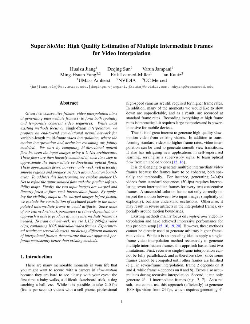
Figure 1: Illustration of intermediate optical flow approxi-mation. The orange pixel borrows optical flow from pixelsat the same position in the first and second images.

the occlusion problem can be addressed. We therefore in-troduce visibility maps Vt←0 and Vt←1. Vt←0(p) ∈ [0, 1]denotes whether the pixel p remains visible (0 is fully oc-cluded) when moving from T = 0 to T = t. Combining thetemporal consistency and occlusion reasoning, we have

It=1

Z�((1−t)Vt←0�g(I0, Ft→0)+tVt←1�g(I1, Ft→1)

),

where Z = (1− t)Vt→0 + tVt→1 is a normalization factor.

3.2. Arbitrary-time Flow InterpolationSince we have no access to the target intermediate image

It, it is hard to compute the flow fields Ft→0 and Ft→1.To address this issue, we can approximately synthesize theintermediate optical flow Ft→0 and Ft→1 using the opticalflow between the two input images F0→1 and F1→0.

Consider the toy example shown in Fig. 1, where eachcolumn corresponds to a certain time step and each dot rep-resents a pixel. For the orange dot p at T = t, we are in-terested in synthesizing its optical flow to its correspondingpixel at T = 1 (the blue dashed arrow). One simple wayis to borrow the optical flow from the same grid positionsat T = 0 and T = 1 (blue and red solid arrows), assumingthat the optical flow field is locally smooth. Specifically,Ft→1(p) can be approximated as

Ft→1(p) = (1− t)F0→1(p) (2)or

Ft→1(p) = −(1− t)F1→0(p), (3)

where we take the direction of the optical flow between thetwo input images in the same or opposite directions andscale the magnitude accordingly ((1− t) in (3)). Similar tothe temporal consistency for RGB image synthesis, we canapproximate the intermediate optical flow by combining thebi-directional input optical flow as follows (in vector form).

Ft→0 = −(1− t)tF0→1 + t2F1→0

Ft→1 = (1− t)2F0→1 − t(1− t)F1→0. (4)

I0 F0→1 F1→0

It Ft→1 Ft→0

I1 Ft→1 Ft→0

‖Ft→1 − Ft→1‖2 ‖Ft→0 − Ft→0‖2

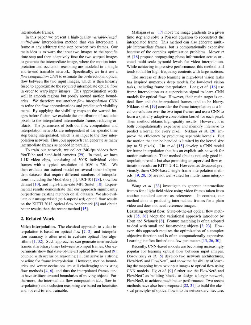
Figure 2: Samples of flow interpolation results, where t =0.5. The entire scene is moving toward the left (due to cam-era translation) and the motorcyclist is independently mov-ing left. The last row shows that the refinement from ourflow interpolation CNN is mainly around the motion bound-aries (the whiter a pixel, the bigger the refinement).

This approximation works well in smooth regions butpoorly around motion boundaries, because the motion nearmotion boundaries is not locally smooth. To reduce artifactsaround motion boundaries, which may cause poor imagesynthesis, we propose learning to refine the initial approx-imation. Inspired by the cascaded architecture for opticalflow estimation in [9], we train a flow interpolation sub-network. This sub-network takes the input images I0 andI1, the optical flows between them F0→1 and F0→1, theflow approximations Ft→0 and F0→1, and two warped in-put images using the approximated flows g(I0, Ft→0) andg(I1, Ft→1) as input, and outputs refined intermediate opti-cal flow fields Ft→1 and Ft→0. Sample interpolation resultsare displayed in Figure 2.

As discussed in Section 3.1, visibility maps are essentialto handle occlusions. Thus, We also predict two visibilitymaps Vt←0 and Vt←1 using the flow interpolation CNN, andenforce them to satisfy the following constraint

Vt←0 = 1− Vt←1. (5)

Without such a constraint, the network training diverges.Intuitively, Vt←0(p) = 0 implies Vt←1(p) = 1, meaningthat the pixel p from I0 is occluded at T = t, we shouldfully trust I1 and vice versa. Note that it rarely happens thata pixel at time t is occluded both at time 0 and 1. Since

I0 I1

Ft→0 Ft→1

g(I0, Ft→0) g(I1, Ft→1)

Vt←0 Vt←1

It It w/o visibility mapsPSNR=30.23 PSNR=30.06

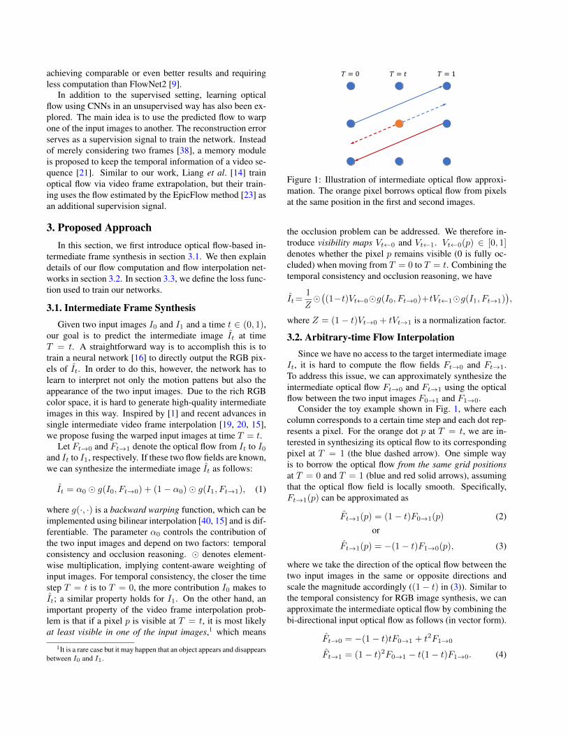
Figure 3: Samples of predicted visibility maps (best viewedin color), where t= 0.5. The arms move downwards fromT =0 to T =1. So the area right above the arm at T =0 isvisible at t but the area right above the arm at T =1 is oc-cluded (i.e., invisible) at t. The visibility maps in the fourthrow clearly show this phenomenon. The white area aroundarms in Vt←0 indicate such pixels in I0 contribute most tothe synthesized It while the occluded pixels in I1 have littlecontribution. Similar phenomena also happen around mo-tion boundaries (e.g., around bodies of the athletes).

we use soft visibility maps, when the pixel p is visible bothin I0 and I1, the network learns to adaptively combine theinformation from two images, similarly to the matting ef-fect [24]. Samples of learned visibility maps are shown in

𝑰𝟎

𝑰𝟏

𝑭𝟎→𝟏

𝑭𝟏→𝟎

𝑭'𝒕→𝟏

𝑭'𝒕→𝟎

𝒈(𝑰𝟎, 𝑭'𝒕→𝟎)

𝑰𝟎

𝒈(𝑰𝟏, 𝑭'𝒕→𝟏)

𝑰𝟏

𝑭𝒕→𝟏

𝑭𝒕→𝟎

𝑽𝒕←𝟎

𝑰𝟏

𝑽𝒕←𝟏

𝑰𝟎

𝑰𝒕

ateachtimestept

flowcomputation arbitrary-timeflowinterpolation

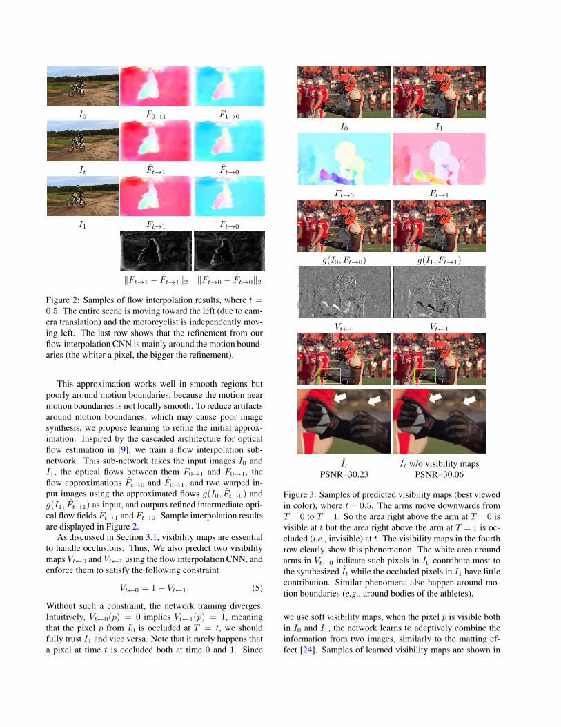
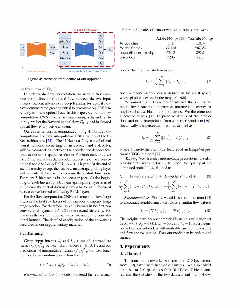
Figure 4: Network architecture of our approach.

the fourth row of Fig. 3.In order to do flow interpolation, we need to first com-

pute the bi-directional optical flow between the two inputimages. Recent advances in deep learning for optical flowhave demonstrated great potential to leverage deep CNNs toreliably estimate optical flow. In this paper, we train a flowcomputation CNN, taking two input images I0 and I1, tojointly predict the forward optical flow F0→1 and backwardoptical flow F1→0 between them.

Our entire network is summarized in Fig. 4. For the flowcomputation and flow interpolation CNNs, we adopt the U-Net architecture [25]. The U-Net is a fully convolutionalneural network, consisting of an encoder and a decoder,with skip connections between the encoder and decoder fea-tures at the same spatial resolution For both networks, wehave 6 hierarchies in the encoder, consisting of two convo-lutional and one Leaky ReLU (α=0.1) layers. At the end ofeach hierarchy except the last one, an average pooling layerwith a stride of 2 is used to decrease the spatial dimension.There are 5 hierarchies in the decoder part. At the begin-ning of each hierarchy, a bilinear upsampling layer is usedto increase the spatial dimension by a factor of 2, followedby two convolutional and Leaky ReLU layers.

For the flow computation CNN, it is crucial to have largefilters in the first few layers of the encoder to capture long-range motion. We therefore use 7×7 kernels in the first twoconvoluional layers and 5 × 5 in the second hierarchy. Forlayers in the rest of entire network, we use 3 × 3 convolu-tional kernels. The detailed configuration of the network isdescribed in our supplementary material.

3.3. Training

Given input images I0 and I1, a set of intermediateframes {Iti}Ni=1 between them, where ti ∈ (0, 1), and ourpredictions of intermediate frames {Iti}Ni=1, our loss func-tion is a linear combination of four terms:

l = λrlr + λplp + λwlw + λsls. (6)

Reconstruction loss lr models how good the reconstruc-

Table 1: Statistics of dataset we use to train our network.

Adobe240-fps [29] YouTube240-fps#video clips 118 1,014#video frames 79,768 296,352mean #frames per clip 670.3 293.1resolution 720p 720p

tion of the intermediate frames is:

lr =1

N

N∑i=1

‖Iti − Iti‖1. (7)

Such a reconstruction loss is defined in the RGB space,where pixel values are in the range [0, 255].

Perceptual loss. Even though we use the L1 loss tomodel the reconstruction error of intermediate frames, itmight still cause blur in the predictions. We therefore usea perceptual loss [11] to preserve details of the predic-tions and make interpolated frames sharper, similar to [20].Specifically, the perceptual loss lp is defined as

lp =1

N

N∑i=1

‖φ(It)− φ(It)‖2, (8)

where φ denote the conv4 3 features of an ImageNet pre-trained VGG16 model [27]

Warping loss. Besides intermediate predictions, we alsointroduce the warping loss lw to model the quality of thecomputed optical flow, defined as

lw =‖I0−g(I1, F0→1)‖1+‖I1−g(I0, F1→0)‖1+ (9)

1

N

N∑i=1

‖Iti−g(I0, Fti→0)‖1+1

N

N∑i=1

‖Iti−g(I1, Fti→1)‖1.

Smoothness loss. Finally, we add a smoothness term [15]to encourage neighboring pixels to have similar flow values:

ls = ‖∇F0→1‖1 + ‖∇F1→0‖1. (10)

The weights have been set empirically using a validation setas λr =0.8, λp =0.005, λw =0.4, and λs =1. Every com-ponent of our network is differentiable, including warpingand flow approximation. Thus our model can be end-to-endtrained.

4. Experiments4.1. Dataset

To train our network, we use the 240-fps videosfrom [29], taken with hand-held cameras. We also collecta dataset of 240-fps videos from YouTube. Table 1 sum-marizes the statistics of the two datasets and Fig. 5 shows

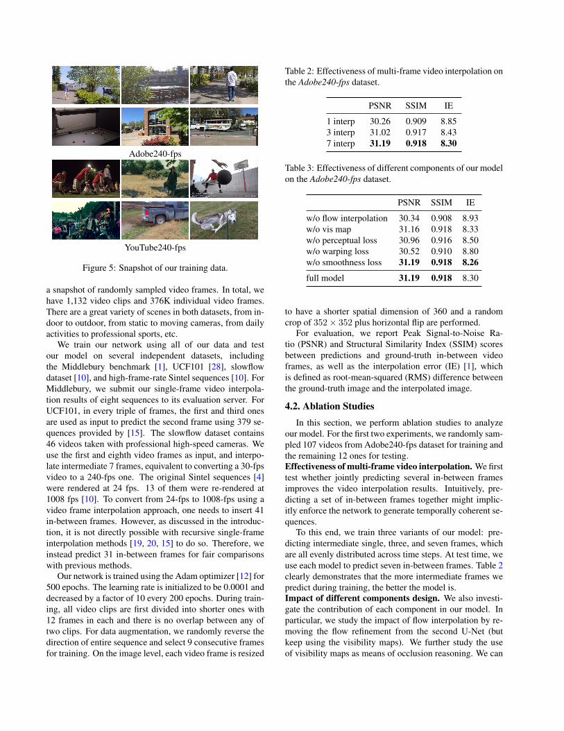
Adobe240-fps

YouTube240-fps

Figure 5: Snapshot of our training data.

a snapshot of randomly sampled video frames. In total, wehave 1,132 video clips and 376K individual video frames.There are a great variety of scenes in both datasets, from in-door to outdoor, from static to moving cameras, from dailyactivities to professional sports, etc.

We train our network using all of our data and testour model on several independent datasets, includingthe Middlebury benchmark [1], UCF101 [28], slowflowdataset [10], and high-frame-rate Sintel sequences [10]. ForMiddlebury, we submit our single-frame video interpola-tion results of eight sequences to its evaluation server. ForUCF101, in every triple of frames, the first and third onesare used as input to predict the second frame using 379 se-quences provided by [15]. The slowflow dataset contains46 videos taken with professional high-speed cameras. Weuse the first and eighth video frames as input, and interpo-late intermediate 7 frames, equivalent to converting a 30-fpsvideo to a 240-fps one. The original Sintel sequences [4]were rendered at 24 fps. 13 of them were re-rendered at1008 fps [10]. To convert from 24-fps to 1008-fps using avideo frame interpolation approach, one needs to insert 41in-between frames. However, as discussed in the introduc-tion, it is not directly possible with recursive single-frameinterpolation methods [19, 20, 15] to do so. Therefore, weinstead predict 31 in-between frames for fair comparisonswith previous methods.

Our network is trained using the Adam optimizer [12] for500 epochs. The learning rate is initialized to be 0.0001 anddecreased by a factor of 10 every 200 epochs. During train-ing, all video clips are first divided into shorter ones with12 frames in each and there is no overlap between any oftwo clips. For data augmentation, we randomly reverse thedirection of entire sequence and select 9 consecutive framesfor training. On the image level, each video frame is resized

Table 2: Effectiveness of multi-frame video interpolation onthe Adobe240-fps dataset.

PSNR SSIM IE

1 interp 30.26 0.909 8.853 interp 31.02 0.917 8.437 interp 31.19 0.918 8.30

Table 3: Effectiveness of different components of our modelon the Adobe240-fps dataset.

PSNR SSIM IE

w/o flow interpolation 30.34 0.908 8.93w/o vis map 31.16 0.918 8.33w/o perceptual loss 30.96 0.916 8.50w/o warping loss 30.52 0.910 8.80w/o smoothness loss 31.19 0.918 8.26

full model 31.19 0.918 8.30

to have a shorter spatial dimension of 360 and a randomcrop of 352× 352 plus horizontal flip are performed.

For evaluation, we report Peak Signal-to-Noise Ra-tio (PSNR) and Structural Similarity Index (SSIM) scoresbetween predictions and ground-truth in-between videoframes, as well as the interpolation error (IE) [1], whichis defined as root-mean-squared (RMS) difference betweenthe ground-truth image and the interpolated image.

4.2. Ablation StudiesIn this section, we perform ablation studies to analyze

our model. For the first two experiments, we randomly sam-pled 107 videos from Adobe240-fps dataset for training andthe remaining 12 ones for testing.Effectiveness of multi-frame video interpolation. We firsttest whether jointly predicting several in-between framesimproves the video interpolation results. Intuitively, pre-dicting a set of in-between frames together might implic-itly enforce the network to generate temporally coherent se-quences.

To this end, we train three variants of our model: pre-dicting intermediate single, three, and seven frames, whichare all evenly distributed across time steps. At test time, weuse each model to predict seven in-between frames. Table 2clearly demonstrates that the more intermediate frames wepredict during training, the better the model is.Impact of different components design. We also investi-gate the contribution of each component in our model. Inparticular, we study the impact of flow interpolation by re-moving the flow refinement from the second U-Net (butkeep using the visibility maps). We further study the useof visibility maps as means of occlusion reasoning. We can

MequonScheffler

UrbanTeddy

BackyardBasketball

DumptruckEvergreen

0

2

4

6

8

10

12

Inte

rpo

latio

n E

rro

r (I

E)

MDP-Flow2PMMSTDeepFlowSepConvOurs

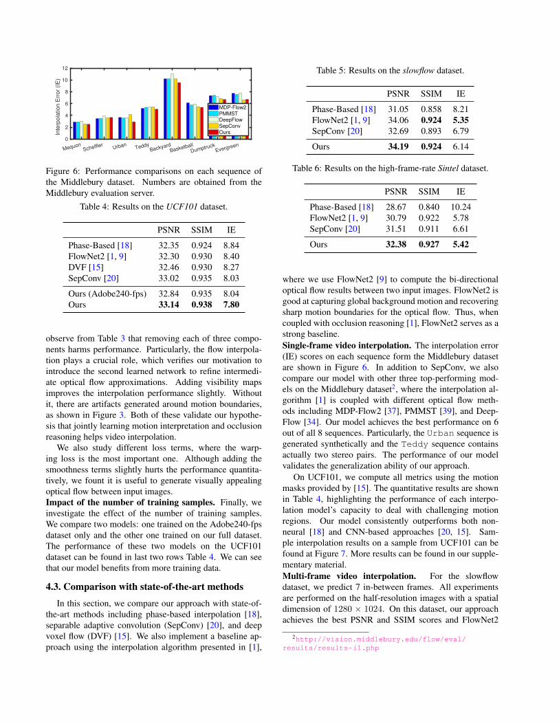
Figure 6: Performance comparisons on each sequence ofthe Middlebury dataset. Numbers are obtained from theMiddlebury evaluation server.

Table 4: Results on the UCF101 dataset.

PSNR SSIM IE

Phase-Based [18] 32.35 0.924 8.84FlowNet2 [1, 9] 32.30 0.930 8.40DVF [15] 32.46 0.930 8.27SepConv [20] 33.02 0.935 8.03

Ours (Adobe240-fps) 32.84 0.935 8.04Ours 33.14 0.938 7.80

observe from Table 3 that removing each of three compo-nents harms performance. Particularly, the flow interpola-tion plays a crucial role, which verifies our motivation tointroduce the second learned network to refine intermedi-ate optical flow approximations. Adding visibility mapsimproves the interpolation performance slightly. Withoutit, there are artifacts generated around motion boundaries,as shown in Figure 3. Both of these validate our hypothe-sis that jointly learning motion interpretation and occlusionreasoning helps video interpolation.

We also study different loss terms, where the warp-ing loss is the most important one. Although adding thesmoothness terms slightly hurts the performance quantita-tively, we fount it is useful to generate visually appealingoptical flow between input images.Impact of the number of training samples. Finally, weinvestigate the effect of the number of training samples.We compare two models: one trained on the Adobe240-fpsdataset only and the other one trained on our full dataset.The performance of these two models on the UCF101dataset can be found in last two rows Table 4. We can seethat our model benefits from more training data.

4.3. Comparison with state-of-the-art methods

In this section, we compare our approach with state-of-the-art methods including phase-based interpolation [18],separable adaptive convolution (SepConv) [20], and deepvoxel flow (DVF) [15]. We also implement a baseline ap-proach using the interpolation algorithm presented in [1],

Table 5: Results on the slowflow dataset.

PSNR SSIM IE

Phase-Based [18] 31.05 0.858 8.21FlowNet2 [1, 9] 34.06 0.924 5.35SepConv [20] 32.69 0.893 6.79

Ours 34.19 0.924 6.14

Table 6: Results on the high-frame-rate Sintel dataset.

PSNR SSIM IE

Phase-Based [18] 28.67 0.840 10.24FlowNet2 [1, 9] 30.79 0.922 5.78SepConv [20] 31.51 0.911 6.61

Ours 32.38 0.927 5.42

where we use FlowNet2 [9] to compute the bi-directionaloptical flow results between two input images. FlowNet2 isgood at capturing global background motion and recoveringsharp motion boundaries for the optical flow. Thus, whencoupled with occlusion reasoning [1], FlowNet2 serves as astrong baseline.Single-frame video interpolation. The interpolation error(IE) scores on each sequence form the Middlebury datasetare shown in Figure 6. In addition to SepConv, we alsocompare our model with other three top-performing mod-els on the Middlebury dataset2, where the interpolation al-gorithm [1] is coupled with different optical flow meth-ods including MDP-Flow2 [37], PMMST [39], and Deep-Flow [34]. Our model achieves the best performance on 6out of all 8 sequences. Particularly, the Urban sequence isgenerated synthetically and the Teddy sequence containsactually two stereo pairs. The performance of our modelvalidates the generalization ability of our approach.

On UCF101, we compute all metrics using the motionmasks provided by [15]. The quantitative results are shownin Table 4, highlighting the performance of each interpo-lation model’s capacity to deal with challenging motionregions. Our model consistently outperforms both non-neural [18] and CNN-based approaches [20, 15]. Sam-ple interpolation results on a sample from UCF101 can befound at Figure 7. More results can be found in our supple-mentary material.Multi-frame video interpolation. For the slowflowdataset, we predict 7 in-between frames. All experimentsare performed on the half-resolution images with a spatialdimension of 1280 × 1024. On this dataset, our approachachieves the best PSNR and SSIM scores and FlowNet2

2http://vision.middlebury.edu/flow/eval/results/results-i1.php

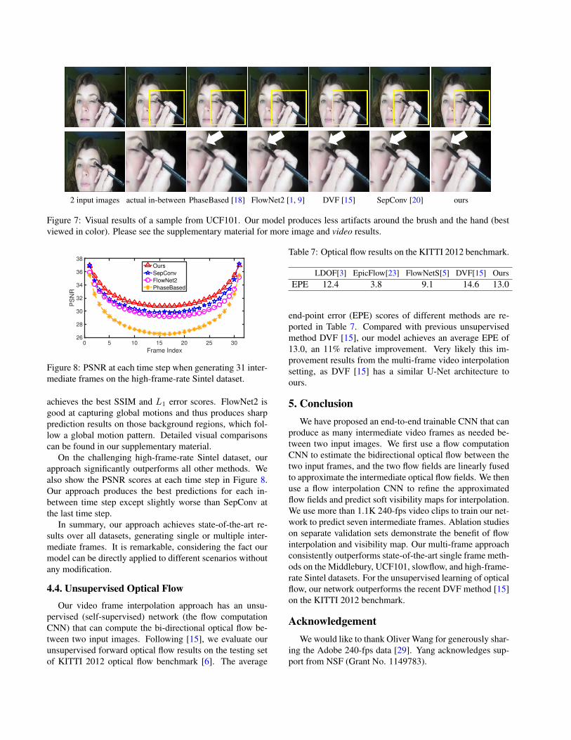
2 input images actual in-between PhaseBased [18] FlowNet2 [1, 9] DVF [15] SepConv [20] ours

Figure 7: Visual results of a sample from UCF101. Our model produces less artifacts around the brush and the hand (bestviewed in color). Please see the supplementary material for more image and video results.

0 5 10 15 20 25 30

Frame Index

26

28

30

32

34

36

38

PS

NR

Ours

SepConv

FlowNet2

PhaseBased

Figure 8: PSNR at each time step when generating 31 inter-mediate frames on the high-frame-rate Sintel dataset.

achieves the best SSIM and L1 error scores. FlowNet2 isgood at capturing global motions and thus produces sharpprediction results on those background regions, which fol-low a global motion pattern. Detailed visual comparisonscan be found in our supplementary material.

On the challenging high-frame-rate Sintel dataset, ourapproach significantly outperforms all other methods. Wealso show the PSNR scores at each time step in Figure 8.Our approach produces the best predictions for each in-between time step except slightly worse than SepConv atthe last time step.

In summary, our approach achieves state-of-the-art re-sults over all datasets, generating single or multiple inter-mediate frames. It is remarkable, considering the fact ourmodel can be directly applied to different scenarios withoutany modification.

4.4. Unsupervised Optical Flow

Our video frame interpolation approach has an unsu-pervised (self-supervised) network (the flow computationCNN) that can compute the bi-directional optical flow be-tween two input images. Following [15], we evaluate ourunsupervised forward optical flow results on the testing setof KITTI 2012 optical flow benchmark [6]. The average

Table 7: Optical flow results on the KITTI 2012 benchmark.

LDOF[3] EpicFlow[23] FlowNetS[5] DVF[15] OursEPE 12.4 3.8 9.1 14.6 13.0

end-point error (EPE) scores of different methods are re-ported in Table 7. Compared with previous unsupervisedmethod DVF [15], our model achieves an average EPE of13.0, an 11% relative improvement. Very likely this im-provement results from the multi-frame video interpolationsetting, as DVF [15] has a similar U-Net architecture toours.

5. ConclusionWe have proposed an end-to-end trainable CNN that can

produce as many intermediate video frames as needed be-tween two input images. We first use a flow computationCNN to estimate the bidirectional optical flow between thetwo input frames, and the two flow fields are linearly fusedto approximate the intermediate optical flow fields. We thenuse a flow interpolation CNN to refine the approximatedflow fields and predict soft visibility maps for interpolation.We use more than 1.1K 240-fps video clips to train our net-work to predict seven intermediate frames. Ablation studieson separate validation sets demonstrate the benefit of flowinterpolation and visibility map. Our multi-frame approachconsistently outperforms state-of-the-art single frame meth-ods on the Middlebury, UCF101, slowflow, and high-frame-rate Sintel datasets. For the unsupervised learning of opticalflow, our network outperforms the recent DVF method [15]on the KITTI 2012 benchmark.

AcknowledgementWe would like to thank Oliver Wang for generously shar-

ing the Adobe 240-fps data [29]. Yang acknowledges sup-port from NSF (Grant No. 1149783).

References[1] S. Baker, D. Scharstein, J. P. Lewis, S. Roth, M. J. Black,

and R. Szeliski. A database and evaluation methodology foroptical flow. IJCV, 92(1):1–31, 2011. 2, 3, 6, 7, 8

[2] J. Barron, D. Fleet, and S. Beauchemin. Performance of op-tical flow techniques. IJCV, 12(1):43–77, 1994. 2

[3] T. Brox and J. Malik. Large displacement optical flow: De-scriptor matching in variational motion estimation. PAMI,33(3):500–513, 2011. 2, 8

[4] D. J. Butler, J. Wulff, G. B. Stanley, and M. J. Black. Anaturalistic open source movie for optical flow evaluation.In ECCV, 2012. 2, 6

[5] A. Dosovitskiy, P. Fischery, E. Ilg, C. Hazirbas, V. Golkov,P. van der Smagt, D. Cremers, T. Brox, et al. Flownet: Learn-ing optical flow with convolutional networks. In ICCV, 2015.2, 8

[6] A. Geiger, P. Lenz, and R. Urtasun. Are we ready for au-tonomous driving? The KITTI vision benchmark suite. InCVPR, 2012. 2, 8

[7] E. Herbst, S. Seitz, and S. Baker. Occlusion reasoning fortemporal interpolation using optical flow. Technical report,August 2009. 2

[8] B. Horn and B. Schunck. Determining optical flow. ArtificialIntelligence, 16:185–203, 1981. 2

[9] E. Ilg, N. Mayer, T. Saikia, M. Keuper, A. Dosovitskiy, andT. Brox. Flownet 2.0: Evolution of optical flow estimationwith deep networks. In CVPR, 2017. 2, 3, 4, 7, 8

[10] J. Janai, F. Guney, J. Wulff, M. Black, and A. Geiger. Slowflow: Exploiting high-speed cameras for accurate and diverseoptical flow reference data. In CVPR, 2017. 2, 6

[11] J. Johnson, A. Alahi, and L. Fei-Fei. Perceptual losses forreal-time style transfer and super-resolution. In ECCV, 2016.5

[12] D. Kingma and J. Ba. Adam: A method for stochastic opti-mization. arXiv preprint arXiv:1412.6980, 2014. 6

[13] Y. Li and D. P. Huttenlocher. Learning for optical flow usingstochastic optimization. In ECCV, 2008. 2

[14] X. Liang, L. Lee, W. Dai, and E. P. Xing. Dual motion GANfor future-flow embedded video prediction. In ICCV, 2017.3

[15] Z. Liu, R. Yeh, X. Tang, Y. Liu, and A. Agarwala. Videoframe synthesis using deep voxel flow. In ICCV, 2017. 1, 2,3, 5, 6, 7, 8

[16] G. Long, L. Kneip, J. M. Alvarez, H. Li, X. Zhang, andQ. Yu. Learning image matching by simply watching video.In ECCV, 2016. 1, 2, 3

[17] D. Mahajan, F.-C. Huang, W. Matusik, R. Ramamoorthi, andP. Belhumeur. Moving gradients: a path-based method forplausible image interpolation. ACM TOG, 28(3):42, 2009. 2

[18] S. Meyer, O. Wang, H. Zimmer, M. Grosse, and A. Sorkine-Hornung. Phase-based frame interpolation for video. InCVPR, 2015. 2, 7, 8

[19] S. Niklaus, L. Mai, and F. Liu. Video frame interpolation viaadaptive convolution. In CVPR, 2017. 1, 2, 3, 6

[20] S. Niklaus, L. Mai, and F. Liu. Video frame interpolation viaadaptive separable convolution. In ICCV, 2017. 1, 2, 3, 5, 6,7, 8

[21] V. Patraucean, A. Handa, and R. Cipolla. Spatio-temporalvideo autoencoder with differentiable memory. In ICLR,workshop, 2016. 3

[22] A. Ranjan and M. J. Black. Optical flow estimation using aspatial pyramid network. In CVPR, 2017. 2

[23] J. Revaud, P. Weinzaepfel, Z. Harchaoui, and C. Schmid.EpicFlow: Edge-Preserving Interpolation of Correspon-dences for Optical Flow. In CVPR, 2015. 2, 3, 8

[24] C. Rhemann, C. Rother, J. Wang, M. Gelautz, P. Kohli, andP. Rott. A perceptually motivated online benchmark for im-age matting. In CVPR, 2009. 4

[25] O. Ronneberger, P. Fischer, and T. Brox. U-net: Convolu-tional networks for biomedical image segmentation. In MIC-CAI, 2015. 5

[26] S. Roth and M. J. Black. On the spatial statistics of opticalflow. IJCV, 74(1):33–50, 2007. 2

[27] K. Simonyan and A. Zisserman. Very deep convolu-tional networks for large-scale image recognition. CoRR,abs/1409.1556, 2014. 5

[28] K. Soomro, A. R. Zamir, and M. Shah. Ucf101: A datasetof 101 human action classes from videos in the wild. CRCV-TR-12-01, 2012. 2, 6

[29] S. Su, M. Delbracio, J. Wang, G. Sapiro, W. Heidrich, andO. Wang. Deep video deblurring. In CVPR, 2017. 2, 5, 8

[30] D. Sun, S. Roth, J. P. Lewis, and M. J. Black. Learningoptical flow. In ECCV, 2008. 2

[31] D. Sun, X. Yang, M.-Y. Liu, and J. Kautz. Pwc-net: Cnnsfor optical flow using pyramid, warping, and cost volume. InCVPR, 2018. 2

[32] R. Szeliski. Prediction error as a quality metric for motionand stereo. In ICCV, 1999. 2

[33] T. Wang, J. Zhu, N. K. Kalantari, A. A. Efros, and R. Ra-mamoorthi. Light field video capture using a learning-basedhybrid imaging system. ACM TOG, 36(4). 2

[34] P. Weinzaepfel, J. Revaud, Z. Harchaoui, and C. Schmid.Deepflow: Large displacement optical flow with deep match-ing. In ICCV, 2013. 7

[35] J. Wulff, L. Sevilla-Lara, and M. J. Black. Optical flow inmostly rigid scenes. In CVPR, 2017. 2

[36] J. Xu, R. Ranftl, and V. Koltun. Accurate optical flow viadirect cost volume processing. In CVPR, 2017. 2

[37] L. Xu, J. Jia, and Y. Matsushita. Motion detail preservingoptical flow estimation. TPAMI, 34(9):1744–1757, 2012. 7

[38] J. J. Yu, A. W. Harley, and K. G. Derpanis. Back to basics:Unsupervised learning of optical flow via brightness con-stancy and motion smoothness. In ECCV, workshop, 2016.3

[39] F. Zhang, S. Xu, and X. Zhang. High accuracy correspon-dence field estimation via mst based patch matching. 2015.7

[40] T. Zhou, S. Tulsiani, W. Sun, J. Malik, and A. A. Efros. Viewsynthesis by appearance flow. In ECCV, 2016. 3