Supercond. Sci. Technol. 28 Modelling current voltage

Modelling current voltage characteristics ofpractical superconductors

A Badía-Majós1 and C López2

1Departamento de Física de la Materia Condensada-I.C.M.A., Universidad de Zaragoza-C.S.I.C., María deLuna 1, E-50018 Zaragoza, Spain2Departamento de Física y Matemáticas, Universidad de Alcalá de Henares, E-28871 Alcalá de Henares,Spain

E-mail: [email protected] and [email protected]

Received 19 June 2014, revised 5 October 2014Accepted for publication 17 October 2014Published 24 December 2014

AbstractBased on recent experimental results, and in the light of fundamental physical properties of themagnetic flux in type-II superconductors, we introduce a practical expression for the material lawto be applied in numerical modelling of superconducting applications. Focusing on thecomputational side, in this paper, previous theory is worked out, so as to take the celebrated formof a power-law-like dependence for the current voltage characteristic. However, contrary to thecommon approach in numerical studies, this proposal suits the general situation of currentdensity flow with components either parallel or perpendicular to the local magnetic field, anddifferent constraints applying on each component. Mathematically, the theory is generated froman elliptic locus defined in terms of the current density vector components. From the physicalside, this contour establishes the boundary for the onset of entropy production related toovercritical current flow in different conditions. The electric field is obtained by partialdifferentiation and points perpendicular to the ellipse. Some numerical examples, inspired by thegeometry of a two-layer helical counter-wound cable are provided. Corrections to the widespreaduse of the implicit isotropic assumption (physical properties only depend on the modulus of thecurrent density vector) are discussed, and essentially indicate that the current carrying capacity ofpractical systems may be underestimated by using such simplification.

Keywords: modelling HTS, critical currents, current voltage

(Some figures may appear in colour only in the online journal)

1. Introduction

Significant progress in the synthesis of superconductingmaterials has recently led to the demand for modelling toolsthat allow the precise simulation of their physical behavior inpotential applications. Thus, a rapid emergence of simulationstudies in electrical machines, solenoids and complex cablegeometries has occurred. However, several issues have beenidentified related to the implementation of computationalcodes at the engineering level, among which a fundamentalquestion remains: Are developers using a sound material law?More specifically, when a conducting sample is subject to acertain process, a standard practice in computational electro-magnetism is to describe its behavior through the so-calledcurrent–voltage characteristic ({V, I} relation) at the

macroscopic level. The concern is whether the formulas usedfor superconductors, that somehow mimic their counterpartfor conventional conductors rely on a solid ground, and towhat extent they can be used in different configurations.

To start with, a basic consensus has been reached that afunctional power-law dependence, i.e.: V is negligibly smallfor transport current values below a certain threshold value(Ic) and quickly increases above, i.e. ∝V I I( )c N , typicallywith ≫N 1, encodes reasonably the observed behavior oftype-II superconductors in the range of applications. More indetail, being concerned with the influence of finite sizeeffects, in many instances, what one typically uses is a localform of the law, i.e.: ρ= J JE J J( ) ( )c N

0 , and further solvesthe Maxwell equations by one or another technique [1]. Thepower-law behavior may be explained as follows. To start

Superconductor Science and Technology

Supercond. Sci. Technol. 28 (2015) 024003 (15pp) doi:10.1088/0953-2048/28/2/024003

0953-2048/15/024003+15$33.00 © 2015 IOP Publishing Ltd Printed in the UK1

with, in the absence of thermal agitation or other statisticaleffects, one has the high exponent limit. This fits the so-calledcritical state regime [2] that describes the sudden transitionsof the flux line lattice, avalanching from one configuration toanother when the flux pinning threshold is exceeded. Thus,speaking of averaged fields over distances containing a largenumber of vortices, true superconducting current flow( ≈E 0) may occur for the subcritical regime ( <J Jc or ‘allvortices are pinned’). However, when the critical currentdensity is exceeded, i.e.: >J Jc some equilibrium conditionsuddenly breaks down and a dissipative regime with a rapidincrease of E starts. On the other hand, either related to finitetemperatures or to inhomogeneous pinning interactions, asmoothing effect takes place, but remarkably, one can still usea power law dependence, now with a reduced value of N [3].The validity of the formula over a noticeable range of electricfield was explained in [4] through the concept of partial fluxflow in the presence of thermal agitation. In practice, oneconsiders it an empirical parameter that may be measured forthe material of interest and in the required ambient conditions.

To the moment, the majority of numerical calculationscomply with such power-law idea and also rely on the so-called isotropic hypothesis that follows on the implicit ansatzof parallelism between the vectors E and J, as indicatedbefore. In fact, as long as the above relation is scalar, one canplainly write it in the form ρ=E J J J J( ) ( )c N

0 that ‘cancelsout’ the corresponding unit vector. Notwithstanding thestraightforward explanation of the power-law dependence, thevalidity of the isotropic behavior is much less clear. Truly,one could find a number of reasons for using this form: (i) itsmathematical simplicity, (ii) the fact that, by using a nonlinearresistivity, it is a minimal upgrade of the normal conductionlaw, and (iii) the satisfactory predictions obtained in manycases, as for long samples in parallel magnetic field. However,contrary to the case of normal conductors, where Ohmʼs lawfinds a natural explanation, in type-II superconductivity,unless for the mentioned geometry, with parallel flux tubes,isotropy is not guaranteed. Without going into detail yet, letus just recall that, according to common knowledge, for thesematerials, the transport properties relate to the drift of the fluxtubes under the action of magnetic forces of the kind ×J B,and this establishes preferential directions in space (in parti-cular those parallel or perpendicular to B). Then, one shouldanalyze if the reasonable predictive power of the isotropic lawis just a stroke of serendipity for other cases. Even more, it iscrucial to detect possible situations in which this ansatz is notacceptable at all. Providing a tool for investigating this fact isthe main motivation of our work, that will be outlined belowin a simple pictorial way. Other interpretations have beendone and will be commented later.

As introduced in previous articles [5], under very generalconditions, the E J( ) law threshold for type-II materials withcomplex flux structures may be described by some closedcontour that is formed by the possible values of the criticalcurrent density vector (critical points J J( , )1 2 in two-dimen-sional (2D) problems at some reference frame, as shown infigure 1). At each point of this map, the electric field arising

by the breakdown of criticality points perpendicular to thecontour. Recall that, excepting the isotropic case (circularcontour) E and J are no longer parallel unless for the specificcases of J pointing along the principal axes. Thus, in practice,the question is to find out whether such a condition is satisfiedor not. As we will see, in many experimental instances theanswer will be positive (or nearly). This is the case for thevast number of experiments in which a uniform magnetic fieldof changing modulus is applied either parallel or perpendi-cular to a flat or very long sample. The screening currents areautomatically perpendicular to the magnetic field and theinduced electric field parallel to the current density. However,for those cases in which the answer is negative, a componentof J parallel to the magnetic field appears, and E is at an anglewith J. Then, it will be important to quantify the eccentricityof the critical contour (a ‘material’ anisotropy of the super-conductor under consideration). Apparently, if the semi-axesare similar enough, one could be confident on the predictionsmade by the isotropic model, that is nothing but the limit inwhich the contour becomes circular.

In brief, this article brings the practical implementation ofthe power-law-elliptic model for the E J( ) material law to beused in superconducting application design. It will be derivedby combination of the power-law concept and the aboveintroduced contour in the elliptic case. The paper is organizedas follows. First, (section 2) we will introduce a physicallymeaningful reference frame for analyzing the critical currentdensity vector. It is given by the local magnetic field vectorand its differential properties. Of particular relevance will beto consider the component of J parallel to the magnetic field.Then, in section 3, having clarified the geometry of Ampèreʼslaw, we will discuss the relation between the physics of type-II superconductors and the above mentioned elliptic region.We will concentrate on various phenomenological issuesrelated to the accurate determination of the specific ellipticregion for a given superconductor from experiment, as well ason the practical expression E J( ). Finally (section 4), in order

Figure 1. Geometrical interpretation of the E J( ) law in a hardsuperconductor. The current density takes ‘critical’ values J J( , )c c1 2

at some contour, while the electric field points perpendicular to suchcontour when the equilibrium breaks down and flux flow occurs. Ingeneral, the problem is defined within some reference frame inwhich J has the components J J( , )1 2 . For homogeneous materials,these components become the projections parallel and perpendicularto the local magnetic field ∥ ⊥J J( , ).

2

Supercond. Sci. Technol. 28 (2015) 024003 A Badía-Majós and C López

to provide some specific tools, as well as for evaluating therelevance of using the correct material law, we give somenumerical examples. The discrete version of a variationalstatement for the power-law-elliptic model is presented andapplied to evaluate the transport properties of helical cableinspired configurations. We concentrate on the influence ofthe basic parameters of the theory: the power law exponent(steepness of the E J( ) dependence), and the eccentricity ofthe ellipse, given by the ratio between the critical currentvalues at different orientations relative to the local mag-netic field.

2. Local geometry of Ampèreʼs law: the normalconducting case

As said before, the relative orientation of the electromagneticfields E J B, , in a superconducting material must be con-sidered with care. Unless for the trivial situation in which themagnetic field is confined to one-dimensional (1D) oscilla-tions, one must expect a situation with screening currents notperpendicular to B and with non-parallel electric fieldsinduced. On the other hand, the selection of an appropriatemacroscopic law has to consider intrinsic geometric proper-ties of the electromagnetic fields, together with the constraintsintroduced by the superconducting interaction. Here, in orderto gain understanding of the problem we start by introducinggeneral requirements for the macroscopic fields showing thata natural reference frame may be introduced to visualize thephysics beyond the trivial situation ∥ ⊥E J B. Then, we willpave the way for the analysis of the superconducting case byfirst studying the simplest problem of linear materials underthe condition ⊥J B.

Being interested in the distinction between the compo-nent of J flowing either parallel or perpendicular to the localmagnetic field, we introduce a reference frame that, for eachpoint of space relies on the differential properties of themagnetic field. This will be useful for interpretative purposes,as well as for simplifying computations. In practice, the usageof this frame will restrict to situations where distinctionbetween the fields B and H is superfluous, i.e.: μ=B H0 . Sothat, no specific consideration is needed for distinctionbetween them.

Consider a generic local magnetic field profile H r( )around a point P, where generic means that the field is neithernull nor constant, and where the gradient of intensity is notaligned with the field, × ≠HH 0. Our aim is to identify thecorrelation between the field and its derivatives with theparallel and perpendicular components of the local currentdensity, according to Ampereʼs law. We will group thesederivatives into mathematically meaningful terms, associatedto the geometric profile of the integral lines of H. In order todo this we start by the factorization = HH h, and considerseparately the derivatives of H and of the unit vector h.

Let us choose a cartesian orthonormal basis (named1 2 3{ˆ , ˆ , ˆ} for generality here) with origin at P, with its firstaxis along PH( ), the second axis on the plane defined by P,

PH( ) and H P( ), and the third axis along ×P H PH( ) ( ).Then, we have =P HH 1( ) ˆ0 and = ∂H P H 1( ) | ˆ

P1 +∂ H 2| ˆP2 .

Around P we have = HH r r h r( ) ( ) ( ), and we can usespherical angles associated to the reference 1 2 3{ˆ , ˆ , ˆ} toexpress the unit vector at and around P, such that

=h r( ) θ ϕr r 1sin ( ) cos ( ) ˆ θ ϕ θ+ +r r 2 r 3sin ( ) sin ( ) ˆ cos ( ) ˆ ,with θ π=P( ) 2 and ϕ =P( ) 0.

A simple example for visualizing this is the case of aninfinite slab with parallel external field (sketched in figure 2).By symmetry, the field is constant (in magnitude and direc-tion) within each parallel plane, so that H must be normal tothese planes and h may rotate in-plane from the surface intothe bulk of the sample. In this case, choosing P at the surfaceand using the global z coordinate to specify the positionwithin the slab: = =z HH 1( 0) ˆ0 , = + =z H z H zH 1 3( ) ( ) ˆ ( ) ˆ1 3

H z zh( ) ( ), with θ θ= +z z zh 1 3( ) sin ( ) ˆ cos ( ) ˆ . The slabapproximation is important because it encodes the mainbehavior of the field in a macroscopic sample, far from cor-ners, edges and curved surfaces. We will use this simplifi-cation in several instances along the article.

Let us proceed with the general expression of Ampèreʼslaw in our reference frame. By applying × = × +HH h

×H h, we get

⎡⎣ ⎤⎦θ ϕ θ ϕ= −∂ + − ∂ + ∂ + ∂ + ∂( )H HJ 3 1 2 3ˆ ˆ ˆ ˆ . (1)2 0 2 3 1 1

Three different geometric terms can be identified:

(i) −∂ H 32 will be denoted screening of intensity. It is themain component of the perpendicular current density,and appears related to the variations of the fieldmodulus. The screening current is normal to bothH andH , so it is in-plane in the slab approximation.

(ii) θ ϕ− ∂ + ∂H 1( ) ˆ0 2 3 represents an helicoidal (or tor-sional) distribution of flux lines around the referenceline through P. This term comes from twisted flux lines(curl) along the directions of the unit vectors 2 or 3, or a

Figure 2. Sketch of the local orthonormal basis 1 2 3{ˆ , ˆ , ˆ} defined interms of the magnetic field and its derivatives for an infinite slabunder parallel magnetic field that changes in modulus andorientation. The dashed line defines the polar angle θ for themagnetic field in the lower plane.

3


sum of both. It is the unique geometric term of the fluxlines correlated to a parallel current density. In the slabapproximation it is also in-plane.

(iii) Finally, θ ϕ∂ + ∂H 2 3( ˆ ˆ)0 1 1 is associated to bending ofthe reference flux line through P, i.e., changes oforientation of the field lines when one ‘walks’ alongthem. The rotation of h can be either in the 1–2 plane(and the term ϕ∂H0 1 is added to the much higher−∂ H2 )or in the 1–3 plane (and θ∂H0 1 correlates to a newnormal component of the current density orthogonal tothe main screening term). Along this article, we willneglect the bending terms to simplify the analysis,understanding that bending is small in the bulk. Indeed,it will vanish exactly in the slab approximation.

The screening current is usually the most relevant inmagnitude, with direct physical interpretation as the reactionof the sample against external variation of the magnetic fieldmodulus. Similarly, the helicoidal current is a screeningreaction of the sample against external variation (rotation) ofh. All this occurs because Faradayʼs law determines theinduction of electric field under variation of magneticinduction. Thus, in a normal metal, parallel and perpendicularcomponents of the electric field generate the correspondingcurrents. The sample reacts, according to the material law

σ=J E0 , against external variations of H.For a better visualization, we will exploit the planar

geometry (see figure 2). Thus, in a slab with fieldH parallel tothe plane and H perpendicular, there are two independentcurrent densities, screening of field intensity variation andparallel screening of field rotation, both currents in-plane.They will be denoted = −∂⊥ HJ 32 and θ= − ∂∥ HJ 10 2 .

Let us consider a metallic infinite slab occupyingthe region − ⩽ ⩽d z d as sketched in figure 2, that issubject to an excitation of the kind =Happlied

ω ωH t H t( sin ( ), cos ( ), 0)0 0 . It is well known that, in termsof the normal metal resistivity, the magnetic diffusionequation reads

μ σ= ∂∂tHH. (2)2

0 0

In figure 3 we visualize the solution of this equation, herefor the boundary conditions specified above. For the readers’sake, we recall that a variety of numerical routines areavailable in different codes that address this problem. In ourcase, we have adapted a MATLAB function designed to solvethe heat equation that formally coincides with ours. Recallthat, upon rotation of the applied magnetic field, a peakedstructure of parallel screening current appears. The peaks,close to the boundaries of the slab will be a feature later to beobserved in superconductors, and clearly ascribed to the lagbetween internal layers and the rotating boundary condition.This simple example allows analytical manipulations that onecan use to better understand the role of ∥J . Thus, starting with

equation (2) it is not difficult to show

= ⇒∂

∂ =( )H H

tJ H· 0 0, (3)

x y

thus ensuring that perpendicularity of H and J is only pos-sible for those processes in which field rotation does notoccur, as argued before.

We want to emphasize that the above discussion on theappearance of components of J parallel to the magnetic fieldis not restricted to linear materials. In fact, it may be extra-polated to the case of nonlinear E J( ) relations and, in parti-cular, to the superconducting power-law. However,specialized numerical methods will be required for the ana-lysis. On the other hand, a relevant distinctive feature for thelatter will be the persistent character of the current densities,that only occur as transients in normal metals.

3. E(J) law for type-II superconductors in non-parallel magnetic fields

A simple analysis based on the infinite slab geometry sket-ched figure 2 together with fundamental concepts of type-IIsuperconductivity will tell us about the specific constraints onany acceptable E J( ) relation when flux rotation occurs. Let usfirst suppose that H0 stands for a uniform field applied to thesuperconducting slab and that the field penetrates in the formof parallel flux tubes. In the standard configuration of a singlecomponent field, the following relations hold:

= = =B z J z E zB 1 J 3 E 3( ) ˆ ; ( ) ˆ ; ( ) ˆ . (4)

For instance, they may be supplemented with a materiallaw of the kind =E E J J( )c N

0 . Increasing the modulus of H0

nucleates more and more vortices that penetrate in the sample,driven by the force ×J B (along the axis named 2). Addi-tionally, the electric field and the magnetic flux velocity areconnected by the celebrated Josephsonʼs relation = ×E B v.

On the contrary, if by virtue of some external process, Bwould rotate within the sample, two striking facts need con-sideration: (i) the rotation of B would produce a parallelcomponent of J, i.e. J1 as said in the previous section. Then aslong as one has ∥E J a component of E parallel to the mag-netic field would also appear, a fact that contradicts Joseph-sonʼs relation. (ii) Contrary to the case for =⊥J J( )3 , anarbitrary value of =∥J J( )1 would be allowed, in a so-calledparallel configuration equilibrium state. In fact, according tothe ‘conventional’ concept that flux lines drift if required bythe magnetic force ×J B, the parallel condition would resultin a force free state with no limit for the supercurrent.

The physical considerations exposed above as well as anumber of interesting collateral concepts are already a clas-sical subject. In fact, motivated by the possibility of achievingvery high practical critical currents, several decades ago, stillin the era of low temperature superconductivity, an intenseresearch activity about the so called ‘longitudinal configura-tions’ (in reference to the appearance of ∥J ) has to be reported.

4


The interested reader may find some selected contributions tothis area, along the years, in [6–15]. As extensively compiledin [16], the main facts can be summarized as follows: (i) inpractice, longitudinal configurations are characterized byincreased (though finite) values of the critical current ∥Jc , (ii)related exotic phenomena as paramagnetic magnetization andnegative resistance are found, (iii) a noticeable electric fieldcomponent along the local magnetic field has been measured,(iv) contrary to the case of ⊥Jc , that is rather well understoodin the language of material pinning forces, no consensusexists yet about the real nature of the critical value ∥Jc . Morein detail, the main topic about the parallel critical currentthreshold is whether the underlying physical mechanism isflux cutting (as considered for a long time) or not. Contrary tosuch hypothesis are the facts that concomitant theoreticalpredictions greatly overestimate the measured values of thisquantity and also the experimental observation that ∥Jc isnoticeably influenced by the pinning center landscape [16].Moreover, as shown in that reference, if one completes thetheory with the concept of pinning torque balance, a reason-able prediction for the parallel critical current threshold is

obtained, together with a natural upgrade of Josephsonʼsrelation Ψ= × +E B v .

Below, we will describe our geometrical interpretation ofthe general critical current problem, including the perpendi-cular as well as the parallel component of Jc. The equivalenceto the description by Matsushita [16] will be established.Eventually, we will introduce the description of the resistiveregime, i.e.: the E J( ) law dealing with the overcriticalbehavior.

3.1. Geometrical formulation of the critical state: critical currentyield region

As introduced before, figure 1 gathers the main features of ourcritical state theory for general problems with ∥Jc and ⊥Jccontributing at any relative strength [17]. Recall that theequilibrium ‘critical states’ of the superconductor are given bya certain ‘yield region’ defined by the admissible endpoints ofthe critical current density vector Jc. Under a certain externalprocess, that induces an instantaneous overcritical condition,Jc moves to another point of the locus, and the updatedequilibrium is defined by the condition that the transient

Figure 3. Evolution of the components of H and J penetrating in a metallic slab (figure 2) as induced by rotation of the applied field. The leftcolumn depicts the applied field vector. To the right, we plot the parallel component of J. Dimensionless units, defined by the maximumapplied field Hm and the ratio H dm have been used.

5


electric field is perpendicular to the contour. No furtherevolution along the perfectly conducting contour occursbecause along such boundary one has ∂ ∝J Et . On the otherhand, the actual shape of the ‘critical’ ⊥ ∥J J( )c c curve isdependent on the underlying physics:

• if one assumes that ∥Jc and ⊥Jc are governed by differentphysical phenomena (as in the cutting/pinning hypoth-esis) the region is a rectangle limited by the points

± ±∥ ⊥J J( , )c c* * , with ∥Jc* and ⊥Jc* being independent

material parameters. This approximation corresponds tothe well-known double critical state model [14], that hasbeen extensively exploited.

• If one assumes that ∥Jc and ⊥Jc relate to the samephysical mechanism, a certain functional relation

⊥ ∥J J( )c c may be established, and one has a contourdefined by some smooth curve. This idea supports theelliptic models [20], a class that includes our currentproposal.

Let us show that, if one follows the simplifying ansatzthat it is one single physical mechanism that fully determinesthe constraint forces that hold flux structures in equilibrium[16], then, the yield region is an ellipse. Although a rigoroustreatment of vortices and their interactions would require toinvoke the Ginzburg–Landau theory, the London approx-imation will suffice for incorporating the relevant ideas. Thus,to start with, we consider that magnetic flux penetrates thesuperconductor in the form of a net of straight, rigid flux tubes(vortices) interacting with each other, with the magnetic field,and possibly with the underlying material. A somewhatlengthy but standard calculation gives the following expres-sion for the vortex lattice free energy, under the action of anexternal field [18, 19]

⎡⎣⎢⎢

⎤⎦

∑ ∑Φ β Φμ λ β β

λ

= − + −

× −<

( ) ( )( )

H l

d

cos cot

exp . (5)

pp

p mp m

pm

0 00

0

Here, βp is the tilt angle for the vortex p relative to theexternal field direction and dpm the (minimum) distancebetween the vortices p and m.

What is important here is to realize that for large mag-netic fields H0 (as compared to the field created by the vor-tices themselves at each point of space) the dominant term foreach individual vortex is βH cos ( )p0 , and the stationary arrayis the well known arrangement of parallel vortices:β = ∀p0 ,p in a regular triangular mesh. On the other hand,in the presence of pinning, stationary configurations ofmagnetic field with non-vanishing current density compo-nents, both perpendicular (gradient of field intensity) andparallel (lack of alignment) may exist. One can say that thevortex–vortex and vortex–external field interactions arebalanced by some ‘vortex-pin’ force and then: (i) the per-pendicular component of the local current density is main-tained in the stationary regime by a pinning force opposed tothe repulsion between vortices. Similarly, (ii) the parallel

component of the current density, associated to misalignmentof flux lines with the external field, is maintained by anopposed pinning torque. This is sketched in figure 4. Thereader is addressed to [16] for a detailed discussion on thephysical origin of torques.

In this scenario, the thresholds for the two components ofJc are related to the projections of a unique pinning forcevector, say F0 either parallel or perpendicular to the plane ofthe slab under consideration: φ φ= F FF ( sin ( ), cos ( )0 0 0 .Assuming linearity in the relation between the forces (tor-ques) and the current densities, that is to say:

φ φ= =∥ ⊥J c F J c Fcos ( ), sin ( )c c1 0 2 0 one arrives at theequilibrium condition

⎛⎝⎜

⎞⎠⎟

⎛⎝⎜

⎞⎠⎟+ =∥ ⊥J

c FJc F

1, (6)c c

1 0

2

2 0

2

where c1 and c2 play the role of phenomenological constants,

Figure 4. Sketch of virtual perturbations of the flux line latticerelative to the configuration of equilibrium. Upper: compression offlux lines. Lower: rotation. Also indicated are the pinning actionsagainst the restoring forces.

6


allowing different critical parameters =∥J c Fc* 1 0, =⊥J c Fc

* 2 0,and thus, magnetic anisotropy3.

In conclusion, the common origin of a total threshold forpinning interaction forces and torques which balance theintrinsic repulsion and alignment, gives way to an ellipticregion of critical supercurrents at each point of the sample,with principal axis parallel and perpendicular to the localfield. Obviously all this refers to the mesoscopic scale, i.e.:after coarse graining in order to smooth fluctuations in thescale of individual vortices.

3.2. Experimental determination: securing the Jc⊥; Jc∥! "

relation

The investigation of general critical states has deservedattention in numerous experiments in the last decades, but ithas not been until recently that a clear evidence of the kind ofmechanism controlling ∥Jc and ⊥Jc has been available. Therelevance of parallel current flow in type-II superconductorswas been tested in a dedicated experiment [20] that, providesdirect information on the threshold (critical) current densitywhen J and B are at an arbitrary angle.

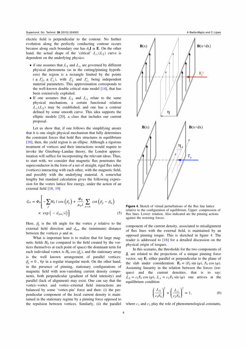
Figure 5 displays the basic features of the experimentalsetup. Owing to the quasi-1D structure of the conductor, andto the negligible self-field effects, the authors could draw aclear picture of the critical current behavior, i.e.: θJ ( )c . Basedon the straightforward measurement of the voltage in theirtransport measurement, they present a set of data for theinduced electric field components θE ( )y and θE ( )z . As afigure of merit, that allows to clearly distinguish betweendifferent models, they plot the ratio θ θE E( ) ( )y z . Basically,the experimental data agree with a dependence of the kind

θ θ Φ θ− + ≡a a a[(1 ) tan ( )] [ tan ( )] ( , )c2 2 2 with a some

constant, as will be later discussed. Such data, supported bycomplementary analysis by Campbell [21] together withdiverse publications that focus on the angular dependences

[22] confirm that an elliptic yield region

θ θ+ =∥ ⊥

J

J

J

J

cos ( ) sin ( )1 (7)c

c

c

c

2 2

* 2

2 2

* 2

is an excellent approximation to the dependence θJ ( )c . Asnoticed by the authors, although the transport measurementprovides a direct information as relates the direction of thecurrent density vector, one has to be careful with the voltagecriterion that are used for determining the ‘critical’ compo-nents. In their experiment, the determination of the ⊥ ∥J J( )c c

critical curve was secured by checking the independence ofthe results when changing the threshold. Here, we add sometheoretical analysis that gives another perspective of theproblem. The question is that transport measurements rely onthe detection of a voltage when the system is driven awayfrom equilibrium ( Δ→ +J J Jc c ) and one is just willing toreconstruct the equilibrium region θJ ( )c . Taking advantage ofthe quasi-linear analysis developed in [5] we have derived thefollowing expression that quantifies the deviation of themeasured critical curve in terms of the voltage criterion:

⎡⎣⎤⎦

θ δ Γ θ Γ δ Φ θ θ Γ

Γ θ θ

= + + −

− +

⊥ ( )( )

( ) ( )j j j

j

, , , 1 sin cos 1

cos sin . (8)

c c c

c

0 0 02

02

303 2 2

Here, we have introduced the dimensionless parametersδ ρ=⊥ ⊥E J( )0 0 , that quantifies the voltage criterion,

θ Γ θ= + +j (1 tan ) ( tan )c2

02 2 , and Γ = ⊥ ∥J J0 0

*0* . The

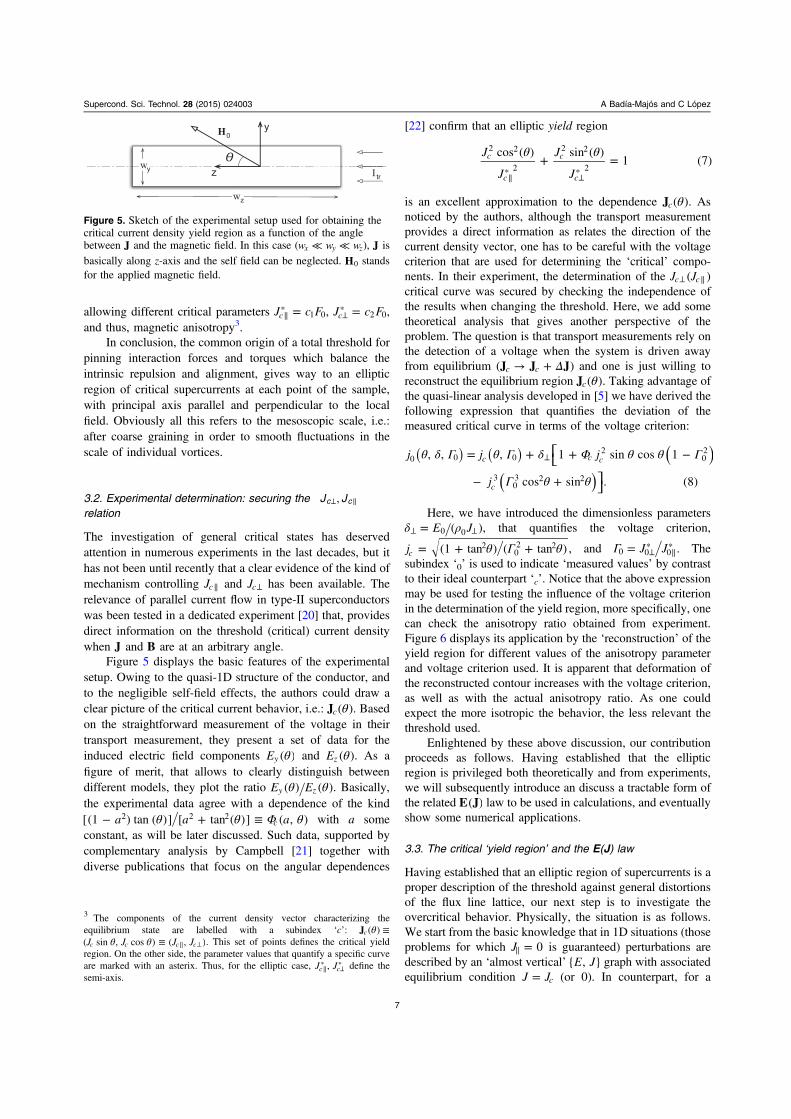
subindex ‘0’ is used to indicate ‘measured values’ by contrastto their ideal counterpart ‘c’. Notice that the above expressionmay be used for testing the influence of the voltage criterionin the determination of the yield region, more specifically, onecan check the anisotropy ratio obtained from experiment.Figure 6 displays its application by the ‘reconstruction’ of theyield region for different values of the anisotropy parameterand voltage criterion used. It is apparent that deformation ofthe reconstructed contour increases with the voltage criterion,as well as with the actual anisotropy ratio. As one couldexpect the more isotropic the behavior, the less relevant thethreshold used.

Enlightened by these above discussion, our contributionproceeds as follows. Having established that the ellipticregion is privileged both theoretically and from experiments,we will subsequently introduce an discuss a tractable form ofthe related E J( ) law to be used in calculations, and eventuallyshow some numerical applications.

3.3. The critical ‘yield region’ and the E(J) law

Having established that an elliptic region of supercurrents is aproper description of the threshold against general distortionsof the flux line lattice, our next step is to investigate theovercritical behavior. Physically, the situation is as follows.We start from the basic knowledge that in 1D situations (thoseproblems for which =∥J 0 is guaranteed) perturbations aredescribed by an ‘almost vertical’ E J{ , } graph with associatedequilibrium condition =J Jc (or 0). In counterpart, for a

Figure 5. Sketch of the experimental setup used for obtaining thecritical current density yield region as a function of the anglebetween J and the magnetic field. In this case ( ≪ ≪w w wx y z), J isbasically along z-axis and the self field can be neglected. H0 standsfor the applied magnetic field.

3 The components of the current density vector characterizing theequilibrium state are labelled with a subindex ‘c’: θ ≡J ( )c

θ θ ≡ ∥ ⊥J J J J( sin , cos ) ( , )c c c c . This set of points defines the critical yieldregion. On the other side, the parameter values that quantify a specific curveare marked with an asterix. Thus, for the elliptic case, ∥ ⊥J J,c c

* * define thesemi-axis.

7


general situation, criticality will be expressed by Ω∈J c (or0) with Ωc the elliptic contour mentioned before. Previously[5], we argued that transients from overcritical points backtowards the region Ωc could be described by a thermo-dynamic dissipation function . This function measures theentropy production and, to the lowest order, is quadratic in theseparation from equilibrium ΔJ . In addition, it was shownthat the electric fields along the dissipative process may beobtained as =E J .

Below, we develop the theory for the power-law exten-sion beyond the elliptic critical state region. In brief, thisentails to identify a mathematical expression for thatintroduces a power-like penalty when J goes beyond theboundary Ωc (see figure 6 for a sketch of the situation). Othermeaningful expressions for as the plain parabolic behaviorhave been checked, but will be discussed elsewhere.

3.3.1. Elliptic-power-law E(J). The starting point for theelliptic-power-law model is the following expression for thedissipation function

⎡

⎣⎢⎢

⎛⎝⎜⎜

⎞⎠⎟⎟

⎛⎝⎜

⎞⎠⎟

⎤

⎦⎥⎥ = +∥

∥

⊥

⊥

J

J

J

JJ( ) . (9)

c c

M

PL 0*

2

*

2

At this point J( )PL is introduced as a reasonable assumptionof a mathematically tractable model that accounts fordissipation when the critical condition represented byequations (6) and (7) is overpassed. A complete theoryrelating the value of M to the flux-pinning properties is out of

reach here. However, it will be shown that some physicalobservables (as the actual angle between E and J) are indeedmodel-independent. Notice also that the ‘partition’ of energydissipation is ensured because by means of the ‘penaltyfunction’ in equation (9) one accounts for virtualdisplacements (figure 6) that can be decomposed as the sumof parallel and perpendicular components, at leastdifferentially. Again, this relies on the idea that a singlephysical mechanism (flux depinning) is the basic limitationfor either conventional or longitudinal configurations. On thepractical side, taking derivatives as dictated by =E Jalong the principal directions, one may easily obtain

γ γ= + +∥−

∥( ) ( )j je j j j( ) . (10)M2 2 1

This formula is a central result of our work, and will bediscussed in detail below. Firstly, dimensionless units havebeen introduced for convenience, through the definitions

γ Γ≡ − ≡ −≡ =≡

⊥ ∥

⊥ ∥ ∥

⊥( )

J J

J j

M J

j J j h

e E

/ * 1 1,

; ,

2 .

(11)c c c

c

c

* 2 2 2

*

0 *

Recall that the anisotropy constant has been reformulatedin terms of the new parameter γ, with the purpose of achievinga compact and meaningful final form for the electric field e.Thus, one can notice that

(i) the isotropic law, i.e. = − jje j( ) ˆM2 1 is obtained in thelimit γ → 0 as expected.

(ii) In those problems for which the parallel current flowmay be neglected ( →∥ ⊥j j 0) one also recovers the

formula = − jje j( ) ˆM2 1 (pseudo-isotropic situation).

As a consistency check, one may calculate the anglebetween the electric field (normal to ϕ) and the currentdensity (normal to α), just by starting with equation (10) andapplying

ϕ α− = e je j

cos ( )·

. (12)

Then

ϕ αΓ α

Γ α− =

−+

( )tan ( )

1 tan ( )

tan ( ). (13)

c

c

2

2 2

Noticeably, this expression coincides exactly with theexpression that was earlier derived for the quasi-linear model[5], and also with the experimental observation reported in[20]. What is more, the angle between the electric field andthe current density happens to be independent of the powerlaw exponent M.

4. Numerical application: examples

In this section, we take a step further in the validation of theelliptic-power-law characteristic. Several numerical examples

Figure 6. Model test of the voltage criterion effect on thereconstruction of the critical current yield region. The upper panel isa sketch the overcritical current (J) that relates to the experiment, aswell as the corresponding ‘real’ critical current density Jc. The lowerpanel shows the actual reconstruction of the critical curves whendifferent voltage criteria δ are used. Specifically, we plot the profilescoming from the set of values δ = 0.01, 0.05, 0.1, 0.2 and for theanisotropy ratios Γ = 1, 0.5, 0.33. For each value of Γ, deformationof the ideal elliptic profile (crosses) increases with δ.

8


will be provided, for which the existence of parallel currentflow is relevant. To start with, we will consider the long-itudinal problem in a strip (experimental setup of figure 5) butnow with the inclusion of a finite width. Secondly, a stackgeometry with different directions for the transport currentalong each element, will be studied, aiming at the basicdescription of helical cable structures. Such configurationshave been extensively treated in the literature [23, 24], but asit will be seen below, noticeable effects due to the appearanceof parallel current flow may occur, that introduce correctionsto the isotropic modelling.

4.1. Quasi-1D analysis of the transport measurementsdetermining Jc(θ)

The analysis of the transport problem described in figure 5was done under the 1D condition ≪ ≪ ⇒ ≈w w w JJ zx y z 0 .Here, we will still consider a long and thin sample, but allowthe appearance of local effects across the width, i.e.: we solvethe transport problem modelled by

≈== −

∥

⊥ ( )

zJ yJ J y h y

J J y h y

J ( ) ˆ( ) ( )

( ) 1 ( ) .

(14)

z

z z

z z2 2 2

Here, hz(y) is the z-component of the unit vector pointingalong the full magnetic field = +H H H0 self . Apparently, thecorrection to the 1D solution will be more important close tothe edges, where the self field effects are more influent on thelocal magnetic field orientation. As said before, an iterativemethod can be used to solve for the y-dependence of Hself ,arising from the distribution jz(y) itself.

Starting from our previous work [5] in which we appliedthe power-law to the pseudo-isotropic situationθ = ° ⇒ =∥J90 0, here we expand the result to the range

θ< < °0 90 . The numerical method described in that work(equations (25) and (26)) has been applied for a dissipationfunction that now reads

γ= +( )h J1 . (15)zM

zM

02 2

In discrete form, hz and Jz are evaluated at a collection ofsegment coordinates = …y i N{ }, 1,i with

= − … =y w y w2, , 2y N y1 . This parametrizes a collection oflong parallel straight wires, each carrying a current Ii. Wehave investigated the resistive transition in terms of the angleθ, by imposing the evolutionary transport condition

∑ θ θ=( ) ( )I t I t, , , (16)i

i 0 tr 0

with θI t( , )tr 0 the increasing value of the transport current at agiven angle θ0 with the applied field. Figure 7 shows the mainfeatures of our results for Γ = 1 3c , the actual value reportedin [20]. (i) To the left, we plot the sheet current profiles thatappear for the extreme condition θ = 0. Notice the increase ofthe transport current density allowed towards the center of thesample. This may be explained in terms of zones whereparallel transport is enhanced. For the smaller applied fields

( =H H5 c0 here), one can see that previous to the full pene-tration regime, a peak may occur, as an indication of the locusof maximum ∥J . For the case =H H50 c0 , the current flow isbasically longitudinal all across the width. (ii) Another aspectthat has to be recalled is the robust behavior of the anisotropydependent quantity ⟨ ⟩ ⟨ ⟩E Ey z against the applied angle. Thus,in spite of the noticeable influence of the voltage criterion inthe actual values of ⟨ ⟩Ey and ⟨ ⟩Ez , the ratio between themaccurately follows the ideal behavior given by the 1D relation(equation (13)) for a wide range of transport levels along thesample.

4.2. Approximation to the helical cable: modelling by planarstacks

Being interested in modelling devices with superconductingcurrents flowing along various regions of space, we start byconsidering the functional analysis problem introduced in[5, 25]. Under magneto-quasi-static conditions, any electro-magnetic process, initiated by manipulation of the sources,may be solved by minimization of the functional

⎡⎣⎢

⎤⎦⎥

∫ ∫∫

∫

πμπΔμ

= ′∥ − ′∥ − ′

∥ − ′∥

+ −

+

+ + +

+ +

∥ + ⊥ +( )

( )

L

tJ J

JJ r J r

r rJ r J r

r r

A A J

ˆ [ ]( ) · ( )

2( ) · ( )

8·

4, . (17)

V V

n n n n

Vn n n

Vn n

dis1 1 1

0e, 1 e, 1

0, 1 , 1

Here, the subindex ‘n’ indicates the value of the quantityfor the time layer tn, Δt is the time interval Δ ≡ −+t t t( )n n1and Ae stands for the vector potential related to the externalsources. Formally, the problem to be solved is: find the vectorfield +Jn 1 (the current density distribution) that minimizes⟨ ⟩L dis subject to the constraints and boundary conditions (inparticular, the values at previous time layer Jn). The addi-tional transport prescription ∫ = IJ s· d tr will have to beapplied if electric current is fed through the superconductor.Recall that the notation ⟨ ⟩L dis is a reminder of the backgroundof the theory: we rely on a modified electromagnetic fieldLagrangian, as discussed in [5, 25]. Recall also that, theelliptic-power-law will be introduced through the specificselection of .

In this section, we have developed the numerical appli-cation of equation (17) for the geometry described in figure 8.As a first approximation to the helical geometry, we introducea planar model that allows a conceptual understanding, aswell as some simple tests against analytical evaluation.Nevertheless, upgrading to the actual cylindrical geometry isstraightforward as will be explained below.

To start with, we notice that as explained by Clem andMalozemoff [24] the inner and outer layers may be solvedseparately in this problem. In fact, the coupling between themonly occurs through a global factor, which is the magneticfield in the intermediate region. This quantity is only depen-dent on the net currents within each superconductor, and noton the actual distribution zJ( ). Let us, thus, concentrate on the

9


outer layers. Due to symmetry, one can just solve one of thetwo slabs (for instance the upper one in our plot). By usingthe coordinates defined in the figure, we state the problem asfollows:

We want to solve equation (17) for a thick slab occupyingthe region < <z d0 (i.e.: V), carrying a transport currentItr along the axis α α(sin , cos , 0)1 1 , and coupled to: (i) anidentical slab with transport along α α−( sin , cos , 0)2 2 ,

Figure 7. Application of the elliptic power-law model to the experiment sketched in figure 5 in the case of a finite width sample under amoderate applied magnetic field at an angle. To the left, the sheet current density across the width of the sample wy. Labels indicate theincreasing values of the transport current in normalized units ( ⊥J w wc x y* ). Also, we use π≡ ⊥H J wc c x* . To the right, we show the averageelectric fields and their ratio as a function of the angle between field and current. The upper pane shows each component at different values ofthe transport current. All curves collapse when one plots their ratio (lower pane) and converge to the 1D relation in equation (13).

Figure 8. Left: sketch of a two-layer counter-wound cylindrical cable built from superconducting tapes. Right: approximation to the cablegeometry by a stack of infinite slabs.

10


and (ii) the field created by two inner slabs also carrying Itreach, but at the angles β1 and β− 2 as shown in figure 8.

This will be done by numerical minimization of thefollowing expression, that is the discrete counterpart

⎡⎣ ⎤⎦

⎡

⎣⎢⎢

⎛⎝⎜⎜

⎞⎠⎟⎟

⎛⎝⎜

⎞⎠⎟

⎤

⎦⎥⎥

∑ ∑

∑ ∑

∑ ∑

∑Δ

= −

+ − +

− + −

+ +∥

∥

⊥

⊥

( )

( )

{ }L I I I I I I

I A A I I

I I I A A

tI

I

I

I

ˆ ,12

˜

˜ 12

˜ ˜

. (18)

ix

iy

i jix

ijxjx

i jix

ijxjx

iix

ex

ex

i jiy

ijy

jy

i jiy

ijy

jy

iiy

ey

ey

i

i

c

i

c

M

dis, ,

,

,

0*

2

*

2

Here, we have used the discretization of V in the form ofa set of parallel layers, each at the position zi, with

= =z z d0 ,..., N1 and constant thickness δ = d N . The layersmay carry current along the x and y axes. In fact, we havedefined the sheet currents along the cartesian axes

δ≡I J z( )ix

x i and δ≡I J z( )iy

y i (our set of N2 unknowns).Also included is the coupling to the applied vector potentialAex y, . Tilded quantities refer to the previous time layer. Dis-

sipation within each sheet is parameterized by the function Fi

that depends on the current components ∥Ii and ⊥Ii . Recall that,for each time step, the evaluation of parallel and perpendi-cular components is performed multiplying by the previouslocal magnetic field, i.e.:

= += −

∥

⊥I I h I h

I I h I h

˜ ˜ ,˜ ˜

(19)i ix

ix

iy

iy

i ix

iy

iy

ix

with hi the unit vector along the magnetic field at zi from theprevious iteration. This quantity must be updated for eachtime step, by application of Ampèreʼs law.

Finally, we have to notice that the ‘mutual inductancecoefficients’ between the layers ij must be dealt with carein this problem. In fact, with our selection of axes, togetherwith the specific orientation for the transport current, one has

⎜ ⎟

⎜ ⎟

⎛⎝

⎞⎠

⎛⎝

⎞⎠

= + ≠

= + −

= + − ≠

= + −

[ ]

i j i j

i

N i j i j

N i

1 2[min { , }] ,

214

1 ,

1 2 max { , } ,

214

.

(20)

ijx

iix

ijy

iiy

As it was discussed in [17], the different expressionshave to do with the symmetry/antisymmetry conditions forthe current flow along each direction. On the other hand,application to the cylindrical geometry would merely consistof replacing these expressions for planar layers by theircounterparts, i.e.: either longitudinal or azimuthal currenttubes.

4.3. Approximation to the helical cable: results

The solution of the problem stated in equation (18) has beenstudied in terms of the main parameters of the elliptic powerlaw model, i.e.: the exponent M and the anisotropy ratioΓ = ⊥ ∥J Jc c

* * . Realistic values in the range of those for HTS atliquid nitrogen temperature have been used. In particular, wehave explored the influence of the power M between 10 and100, and compared the isotropic hypothesis (Γ = 1) to thevalues Γ = 1 2 and Γ = 1 4 that are close around Γ ≈ 1 3obtained in [20] for a patterned YBCO film. Our main find-ings are summarized in figures 9–12.

4.3.1. Influence of the power law exponent M. Figure 9shows a collection of two dimensional maps that, on the oneside assess the validity of our numerical method. Notice that,as expected, the dissipation function restriction introduced inour variational model, gives place to a concentration of pointsclose around the elliptic (in this case, circular) yield region.The higher the value of M, the narrower the region ‘explored’by the sample, eventually becoming a thin line when in thecritical state limit ( ≫M 1). On the other side, one can alsorealize that the appearance of dissipation produces distinctivefeatures in the ∥ ⊥[ , ] or x y[ , ] plots. In the former case, thestates beyond full penetration (i.e.: the critical current hasbeen exceeded) are characterized by a narrow band of valuesof constant J modulus that rotates as M increases. In the x y[ , ]plots, the concentration of overcritical points appears aroundthe vertical axis (along which transport was addressed inthis case).

4.3.2. Influence of the anisotropy parameter Γ. Two aspectshave been analyzed as regards the influence of the ratiobetween the parallel and perpendicular critical current valuesΓ = ⊥ ∥J Jc c

* * . Firstly, as shown in figure 10, we concentrate onthe magnetic hysteresis loops predicted for the currentscirculating along the outer superconducting layer. The mainpurpose of this simulation was to evaluate how stronglyanisotropy affects the shapes of the loops and, as aconsequence, the electromagnetic losses. In particular wehave evaluated the magnetic moment per unit area of the slabas

∫= ×z zm Jd . (21)d

0

A number of distinctive features are to be recalled for theac process generated by the transport current cycle

ω=I I tsin ( )tr 0 .

(i) Only for the case Γ = 1 a collapse of the loop mx isobserved. The absence of hysteresis indicates that theprofile of current density has reached the dissipationlimit, i.e.: −J Jc lies beyond the contour Ωc all aroundthe material.

(ii) The anisotropic cases show a feature in the form of akink in the loops, that shows up close to the condition

=I 0tr . This feature is a clear indication of theincreased value of ∥J and thus can be used as a test of

11


the appearance of intrinsic anisotropy Remarkably, suchbehavior was reported in early experiments withlongitudinal fields [26]. In order to clarify thisinterpretation we include a plot of the components ofH, as well as the profiles of J (figure 11). The readermay notice the increased shielding (higher slope ofhx(z)) that is related to a peak in the current density.This peak occurs at the region of the superconductor,where Hx is close to zero, then rotation predominatesand Jy basically coincides with the parallel component( ≈∥J Jy). Recall the similar phenomenon in figure 3 forthe case of a normal metal. The difference here is thatthe peak of parallel current sits upon the step-like‘critical state’ step profiles.

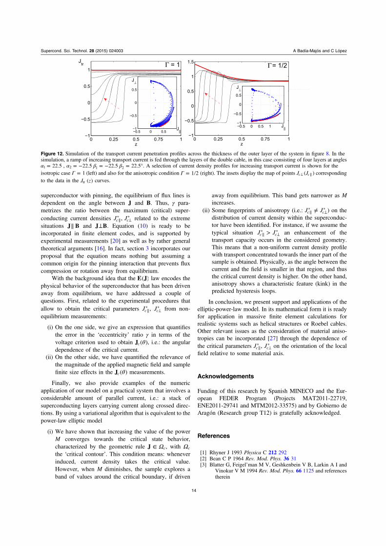
The second aspect to be recalled as regards the influenceof Γ is compiled in figure 12. Here, we show the actualprofiles of the transport current in the helical cable geometry,as one passes over the dissipation condition in a simulationthat feeds a ramp of transport current along the sample.Noticeably, the transport profile in the isotropic situation goesfrom what is basically a step function below dissipation,towards a flat profile that fills the sample (and eventually goesbeyond Jc) if more current is supplied. On the contrary, forthe anisotropic case, the intermediate profiles display apeaked structure, and eventually become monotonous in the

dissipation regime beyond the critical value. The currentflows preferentially along the inner layers of the tape, onceagain advantaged by the parallel current condition. This effectmay be explained through the predominance of self-fieldeffects close to the periphery of the sample, in such a way thatparallel current flow is enhanced towards the center.

5. Concluding remarks

The aim of this work was to provide a reliable expression ofthe material law to be used in wide range simulations ofsuperconducting applications. More specifically:

(i) we have addressed the (frequently bypassed) questionof modelling problems for which the current density ismanifestly non-perpendicular to the magnetic field.

(ii) we have proposed to use a modified version of thepopular power-law E J( ) formula.

The main result of the paper is equation (10):

γ γ= + +∥−

∥( )j je j j j( ) ( )M2 2 1

with j the dimensionlesscurrent density and ∥j its projection onto the local magneticfield. We name it after ‘elliptic-power-law’ model. Thisexpression incorporates the well reported fact that in a type-II

Figure 9. 2D plot of the region ‘explored’ by the superconducting slab (figure 8) that is fed through with an ac transport current of amplitude=I Ictr, max . Each dot represents a point in J-space that has occurred somewhere within the material. The upper plots correspond to the local

axes relative to the field direction and its normal ∥ ⊥[ , ]. The lower pane shows the counterpart for the same conditions, but in terms of theglobal x y[ , ] components. Each column corresponds to a given value of the exponent M as labelled. In all cases, the isotropic condition Γ = 1was used. For this simulation, the angles defined in figure 8 take the values α α= = 01 2 and β β= = °901 2 . J is given in units of ⊥Jc* .

12


Figure 10.Magnetization loops related to the currents circulating along the outer superconducting layer for the system defined in figure 8. Acyclic process of the transport current along the system was assumed that produces a magnetic field h h( , )x y0 0 in the intermediate region.H is

given in units of ⊥J d 2c* , and the magnetic moment in units of ⊥J d 4c

* 2 with d the thickness of the slab. Here, we have usedα α β β= = = = °0 , 67.51 2 1 2 .

Figure 11. Profiles of the magnetic field and current density penetrating the superconductor in the configuration studied in figure 10, for thecase Γ = 1 2.H is given in units of ⊥J d 2c

* , J in units of ⊥Jc* and z normalized to the width d. z = 0 means the inner part of the slab. The arrowindicates the evolution of the boundary conditions.

13


superconductor with pinning, the equilibrium of flux lines isdependent on the angle between J and B. Thus, γ para-metrizes the ratio between the maximum (critical) super-conducting current densities ∥ ⊥J J,c c

* * related to the extremesituations ∥J B and ⊥J B. Equation (10) is ready to beincorporated in finite element codes, and is supported byexperimental measurements [20] as well as by rather generaltheoretical arguments [16]. In fact, section 3 incorporates ourproposal that the equation means nothing but assuming acommon origin for the pinning interaction that prevents fluxcompression or rotation away from equilibrium.

With the background idea that the E J( ) law encodes thephysical behavior of the superconductor that has been drivenaway from equilibrium, we have addressed a couple ofquestions. First, related to the experimental procedures thatallow to obtain the critical parameters ∥Jc* , ⊥Jc* from non-equilibrium measurements:

(i) On the one side, we give an expression that quantifiesthe error in the ‘eccentricity’ ratio γ in terms of thevoltage criterion used to obtain θJ ( )c , i.e.: the angulardependence of the critical current.

(ii) On the other side, we have quantified the relevance ofthe magnitude of the applied magnetic field and samplefinite size effects in the θJ ( )c measurements.

Finally, we also provide examples of the numericapplication of our model on a practical system that involves aconsiderable amount of parallel current, i.e.: a stack ofsuperconducting layers carrying current along crossed direc-tions. By using a variational algorithm that is equivalent to thepower-law elliptic model

(i) We have shown that increasing the value of the powerM converges towards the critical state behavior,characterized by the geometric rule Ω∈J c, with Ωc

the ‘critical contour’. This condition means: wheneverinduced, current density takes the critical value.However, when M diminishes, the sample explores aband of values around the critical boundary, if driven

away from equilibrium. This band gets narrower as Mincreases.

(ii) Some fingerprints of anisotropy (i.e.: ≠∥ ⊥J Jc c* * ) on the

distribution of current density within the superconduc-tor have been identified. For instance, if we assume thetypical situation >∥ ⊥J Jc c

* * an enhancement of thetransport capacity occurs in the considered geometry.This means that a non-uniform current density profilewith transport concentrated towards the inner part of thesample is obtained. Physically, as the angle between thecurrent and the field is smaller in that region, and thusthe critical current density is higher. On the other hand,anisotropy shows a characteristic feature (kink) in thepredicted hysteresis loops.

In conclusion, we present support and applications of theelliptic-power-law model. In its mathematical form it is readyfor application in massive finite element calculations forrealistic systems such as helical structures or Roebel cables.Other relevant issues as the consideration of material aniso-tropies can be incorporated [27] through the dependence ofthe critical parameters ∥ ⊥J J,c c

* * on the orientation of the localfield relative to some material axis.

Acknowledgements

Funding of this research by Spanish MINECO and the Eur-opean FEDER Program (Projects MAT2011-22719,ENE2011-29741 and MTM2012-33575) and by Gobierno deAragón (Research group T12) is gratefully acknowledged.

References

[1] Rhyner J 1993 Physica C 212 292[2] Bean C P 1964 Rev. Mod. Phys. 36 31[3] Blatter G, Feigel’man M V, Geshkenbein V B, Larkin A I and

Vinokur V M 1994 Rev. Mod. Phys. 66 1125 and referencestherein

Figure 12. Simulation of the transport current penetration profiles across the thickness of the outer layer of the system in figure 8. In thesimulation, a ramp of increasing transport current is fed through the layers of the double cable, in this case consisting of four layers at anglesα α β β= = − = − = °22.5 , 22.5 22.5 22.51 2 1 2 . A selection of current density profiles for increasing transport current is shown for theisotropic case Γ = 1 (left) and also for the anisotropic condition Γ = 1 2 (right). The insets display the map of points ⊥ ∥J J( )c c correspondingto the data in the J z( )tr curves.

14


[4] Yamafuji K and Kiss T 1997 Physica C 290 9[5] Badía-Majós A and López C 2012 Supercond. Sci. Technol. 25

104004[6] Campbell A M and Evetts J E 1972 Adv. Phys. 21 199 and

references therein[7] Walmsley D G 1971 J. Phys. F: Met. Phys. 2 510

Walmsley D G and Timms W E 1977 J. Phys. F: Met. Phys.7 2373

[8] Cave J R and Evetts J E 1978 Phil. Mag. B 37 111[9] Matsushita T, Shimogawa A and Asano M 1998 Physica C

298 115[10] Clem J R 1980 J. Low Temp. Phys. 38 353

Brandt E H 1980 J. Low Temp. Phys. 39 41[11] Voloshin I F et al 1991 JEPT Lett. 53 115[12] Fisher L M et al 1997 Solid State Commun. 103 313[13] LeBlanc M A R, Celebi S, Wang S X and Plechacek V 1993

Phys. Rev. Lett. 71 3367[14] Clem J R and Pérez-González A 1984 Phys. Rev. B 30 5041[15] Ruiz H S, López C and Badía A 2011 Phys. Rev. B 83 014506[16] Matsushita T 2014 Flux Pinning in Superconductors (Berlin:

Springer)Matsushita T 2012 Japan. J. Appl. Phys. 51 010111

[17] Badía-Majós A, López C and Ruiz H S 2009 Phys. Rev. B 80144509

[18] Brandt E H, Clem J R and Walmsley D G 1979 J. Low Temp.Phys. 37 43

[19] Orlando T P and Delin K A 1991 Foundations of AppliedSuperconductivity (Englewood Cliffs, NJ: Prentice-Hall)

[20] Clem J R, Weigand M, Durrell J H and Campbell A M 2011Supercond. Sci. Technol. 24 062002

[21] Campbell A M 2011 Supercond. Sci. Technol. 24 091001[22] Pitel J and Kováč P 2011 Physica C 471 1680[23] Nii M, Amemiya N and Nakamura T 2012 Supercond. Sci.

Technol. 25 095011Zermeno V M, Grilli F and Sirois F 2013 Supercond. Sci.

Technol. 26 052001[24] Clem J R and Malozemoff A P 2010 Supercond. Sci. Technol.

23 034014[25] Badía-Majós A, Cariñena J F and López C 2009 J. Phys. A:

Math. Theor. 39 14699[26] Walmsley D G 1972 J. Phys. F: Met. Phys. 2 510[27] Amigo M L, Ale Crivillero V, Franco D G, Badía-Majós A,

Guimpel J and Nieva G 2014 J. Phys.: Conf. Ser. 507012001

15


Documents

Supercond. Sci. Technol. 28 Modelling current voltage