Superconducting Circuits for Quantum Information: An Outlookqulab.eng.yale.edu/documents/Superconducting_Circuits... · 2020-02-08 · Superconducting circuits 1 Superconducting Circuits

Superconducting circuits

1

Superconducting Circuits for Quantum Information: An Outlook*

M. H. Devoret and R. J. Schoelkopf

Applied Physics and Physics Departments, Yale University

The performance of superconducting qubits has improved by several orders of magnitude

in the past decade. These circuits benefit from the robustness of superconductivity and

the Josephson effect, and at present they have not encountered any fundamental physical

limits. However, building an error-corrected information processor with many such

qubits will require solving specific architecture problems that constitute a new field of

research. For the first time, physicists will have to master quantum error correction to

design and operate complex active systems that are dissipative in nature, yet remain

coherent indefinitely. We offer a view on some directions for the field and speculate on

its future.

The concept of solving problems with the use of quantum algorithms, introduced in the

early 1990s1,2

, was welcomed as a revolutionary change in the theory of computational

complexity, but the feat of actually building a quantum computer was then thought to be

impossible. The invention of quantum error correction (QEC)3,4,5,6

introduced hope that a

quantum computer might one day be built, most likely by future generations of physicists

and engineers. However, less than 20 years later, we have witnessed so many advances

that successful quantum computations, and other applications of quantum information

processing (QIP) such as quantum simulation7,8

and long-distance quantum

communication9, appear reachable within our lifetime, even if many discoveries and

technological innovations are still to be made.

Below, we discuss the specific physical implementation of general-purpose QIP with

superconducting qubits10

. A comprehensive review of the history and current status of the

field is beyond the scope of this article. Several detailed reviews on the principles and

operations of these circuits already exist11,12,13,14

. Here, we raise only a few important

aspects needed for the discussion before proceeding to some speculations on future

directions.

Toward a Quantum Computer

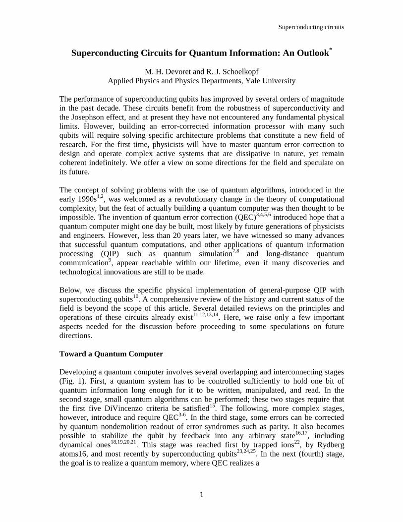
Developing a quantum computer involves several overlapping and interconnecting stages

(Fig. 1). First, a quantum system has to be controlled sufficiently to hold one bit of

quantum information long enough for it to be written, manipulated, and read. In the

second stage, small quantum algorithms can be performed; these two stages require that

the first five DiVincenzo criteria be satisfied15

. The following, more complex stages,

however, introduce and require QEC3-6

. In the third stage, some errors can be corrected

by quantum nondemolition readout of error syndromes such as parity. It also becomes

possible to stabilize the qubit by feedback into any arbitrary state16,17

, including

dynamical ones18,19,20,21

. This stage was reached first by trapped ions22

, by Rydberg

atoms16, and most recently by superconducting qubits23,24,25

. In the next (fourth) stage,

the goal is to realize a quantum memory, where QEC realizes a


2

Fig. 1. Seven stages in the development of quantum information processing. Each advancement

requires mastery of the preceding stages, but each also represents a continuing task that must be

perfected in parallel with the others. Superconducting qubits are the only solid-state

implementation at the third stage, and they now aim at reaching the fourth stage (green arrow). In

the domain of atomic physics and quantum optics, the third stage had been previously attained by

trapped ions and by Rydberg atoms. No implementation has yet reached the fourth stage, where a

logical qubit can be stored, via error correction, for a time substantially longer than the

decoherence time of its physical qubit components.

coherence time that is longer than any of the individual components. This goal is as yet

unfulfilled in any system. The final two stages in reaching the ultimate goal of fault-

tolerant quantum information processing26

require the ability to do all single qubit

operations on one logical qubit (which is an effective qubit protected by active error

correction mechanisms), and the ability to perform gate operations between several

logical qubits; in both stages the enhanced coherence lifetime of the qubits should be

preserved.

Superconducting Circuits: Hamiltonians by Design

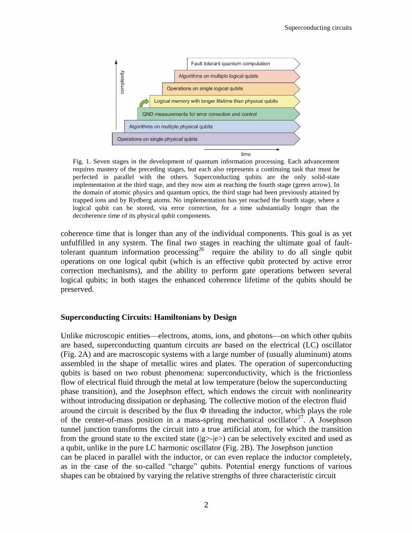
Unlike microscopic entities—electrons, atoms, ions, and photons—on which other qubits

are based, superconducting quantum circuits are based on the electrical (LC) oscillator

(Fig. 2A) and are macroscopic systems with a large number of (usually aluminum) atoms

assembled in the shape of metallic wires and plates. The operation of superconducting

qubits is based on two robust phenomena: superconductivity, which is the frictionless

flow of electrical fluid through the metal at low temperature (below the superconducting

phase transition), and the Josephson effect, which endows the circuit with nonlinearity

without introducing dissipation or dephasing. The collective motion of the electron fluid

around the circuit is described by the flux threading the inductor, which plays the role

of the center-of-mass position in a mass-spring mechanical oscillator27

. A Josephson

tunnel junction transforms the circuit into a true artificial atom, for which the transition

from the ground state to the excited state (|g>-|e>) can be selectively excited and used as

a qubit, unlike in the pure LC harmonic oscillator (Fig. 2B). The Josephson junction

can be placed in parallel with the inductor, or can even replace the inductor completely,

as in the case of the so-called “charge” qubits. Potential energy functions of various

shapes can be obtained by varying the relative strengths of three characteristic circuit


3

Fig. 2. (A) Superconducting qubits consist of simple circuits that can be described as the parallel

combination of a Josephson tunnel element (cross) with inductance LJ, a capacitance C, and an

inductance L. The flux F threads the loop formed by both inductances. (B) Their quantum energy

levels can be sharp and long lived if the circuit is sufficiently decoupled from its environment. The

shape of the potential seen by the flux F and the resulting level structure can be varied by changing

the values of the electrical elements. This example shows the fluxonium parameters, with an

imposed external flux of 1/4 flux quantum. Only two of three corrugations are shown fully. (C) A

Mendeleev-like but continuous “table” of artificial atom types: Cooper pair box29

, flux qubit33

,

phase qubit35

, quantronium37

, transmon39

, fluxonium40

, and hybrid qubit41

. The horizontal and

vertical coordinates correspond to fabrication parameters that determine the inverse of the number

of corrugations in the potential and the number of levels per well, respectively.

energies associated with the inductance, capacitance, and tunnel element (Fig. 2, B and

C). Originally, the three basic types were known as charge28,29

, flux30,31,32,33

, and

phase34,35

. The performance of all types of qubits has markedly improved as the

fabrication, measurement, and materials issues affecting coherence have been tested,

understood, and improved.

In addition, there has been a diversification of other design variations, such as the

quantronium36,37

, transmon38,39

, fluxonium40

, and “hybrid”41

qubits; all of these are

constructed from the same elements but seek to improve performance by reducing their

sensitivity to decoherence mechanisms encountered in earlier designs. The continuing

evolution of designs is a sign of the robustness and future potential of the field.

When several of these qubits, which are nonlinear oscillators behaving as artificial atoms,

are coupled to true oscillators (photons in a microwave cavity), one obtains, for low-lying

excitations, an effective multiqubit, multicavity system Hamiltonian of the form

2

† † † † †

,

,

/ / 2q r

eff j j j j j j m m m j m j j m m

j m j m

H b b b b a a b b a a

describing anharmonic qubit mode amplitudes indexed by j coupled to harmonic cavity

modes indexed by m42

. The symbols a, b, and refer to the mode amplitudes and

frequency, respectively. When driven with appropriate microwave signals, this system


4

can perform arbitrary quantum operations at speeds determined by the nonlinear

interaction strengths and , typically43,44

resulting in single-qubit gate times within 5 to

50 ns (/2 ≈ 200 MHz) and two qubit entangling gate times within 50 to 500 ns (/2 ≈

20 MHz). We have neglected here the weak induced anharmonicity of the cavity modes.

Proper design of the qubit circuit to minimize dissipation coming from the dielectrics

surrounding the metal of the qubit, and to minimize radiation of energy into other

electromagnetic modes or the circuit environment, led to qubit transition quality factors Q

exceeding 1 million or coherence times on the order of 100 ms, which in turn make

possible hundreds or even thousands of operations in one coherence lifetime (see

Table 1). One example of this progression, for the case of the Cooper-pair box (28) and

its descendants, is shown in Fig. 3A. Spectacular improvements have also been

accomplished for transmission line resonators45

and the other types of qubits, such the

phase qubit35

or the flux qubit46

. Rather stringent limits can now be placed on the intrinsic

capacitive47

or inductive43

losses of the junction, and we construe this to mean that

junction quality is not yet the limiting factor in the further development of

superconducting qubits.

Nonetheless, it is not possible to reduce dissipation in a qubit independently of its readout

and control systems39

. Here, we focus on the most useful and powerful type of readout,

which is called a “quantum nondemolition” (QND) measurement. This type of

measurement allows a continuous monitoring of the qubit state48,49

. After a strong QND

measurement, the qubit is left in one of two computational states, |g> or |e>, depending

on the result of the measurement, which has a classical binary value indicating g or e.

There are three figures of merit that characterize this type of readout. The first is QND-

ness, the probability that the qubit remains in the same state after the measurement, given

that the qubit is initially in a definite state |g> or |e>. The second is the intrinsic fidelity,

the difference between the probabilities—given that the qubit is initially in a definite state

|g> or |e>—that the readout gives the correct and wrong answers (with this definition, the

fidelity is zero when the readout value is uncorrelated with the qubit state). The last and

most subtle readout figure of merit is efficiency, which characterizes the ratio of the

number of controlled and uncontrolled information channels in the readout. Maximizing

this ratio is of utmost importance for performing remote entanglement by measurement50

.

Like qubit coherence, and benefiting from it, progress in QND performance has been

spectacular (Fig. 3B). It is now possible to acquire more than N = 2000 bits of

information from a qubit before it decays through dissipation (Fig. 3A), or, to phrase it

more crudely, read a qubit once in a time that is a small fraction (1/N) of its lifetime. This

is a crucial capability for undertaking QEC in the fourth stage of Fig. 1, because in order

to fight errors, one has to monitor qubits at a pace faster than the rate at which they occur.

Efficiencies in QND superconducting qubit readout are also progressing rapidly and will

soon routinely exceed 0.5, as indicated by recent experiments25,51

.

Is It Just About Scaling Up?

Up to now, most of the experiments have been done on a relatively small scale, involving

only a handful of interacting qubits or degrees of freedom; see Table 1. Furthermore,

almost all the experiments so far are “passive”—they seek to maintain coherence only

long enough to entangle quantum bits or demonstrate some rudimentary capability


5

before, inevitably, decoherence sets in. The next stages of QIP require one to realize an

actual increase in the coherence time via error correction, first only during an idle

“memory” state, but later also in the midst of a functioning algorithm. This requires

building new systems that are “active,” using continuous measurements and real-time

feedback to preserve the quantum information through the startling process of correcting

qubit errors without actually learning what the computer is calculating. Given the

fragility of quantum information, it is commonly believed that the continual task of error

correction will occupy the vast majority of the effort and the resources in any large

quantum computer.

Using the current approaches to error correction, the next stages of development

unfortunately demand a substantial increase in complexity, requiring dozens or even

thousands of physical qubits per bit of usable quantuminformation, and challenging our

currently limited abilities to design, fabricate, and control a complex Hamiltonian

(second part of Table 1). Furthermore, all of the DiVincenzo engineering margins on

each piece of additional hardware still need to be maintained or improved while scaling

up. So is advancing to the next stage just a straightforward engineering exercise of mass-

producing large numbers of exactly the same kinds of circuits and qubits that have

already been demonstrated? And will this mean the end of the scientific innovations that

have so far driven progress forward?

We argue that the answers to both questions will probably be “No.” The work by the

community during the past decade and a half, leading up to the capabilities summarized

in the first part of Table 1, may indeed constitute an existence proof that building a large-

scale quantum computer is not physically impossible. However, identifying the best, most

efficient, and most robust path forward in a technology’s development is a task very

different from merely satisfying oneself that it should be possible. So far, we have yet to

see a dramatic “Moore’s law” growth in the complexity of quantum hardware. What,

then, are the main challenges to be overcome?

Simply fabricating a wafer with a large number of elements used today is probably not

the hard part. After all, some of the biggest advantages of superconducting qubits are that

they are merely circuit elements, which are fabricated in clean rooms, interact with each

other via connections that are wired up by their designer, and are controlled and

measured from the outside with electronic signals. The current fabrication requirements

for superconducting qubits are not particularly daunting, especially in comparison to

modern semiconductor integrated circuits (ICs). A typical qubit or resonant cavity is a

few millimeters in overall size, with features that are mostly a few micrometers (even the

smallest Josephson junction sizes are typically 0.2 mm on a side in a qubit). There is

successful experience with fabricating and operating superconducting ICs with hundreds

to thousands of elements on a chip, such as the transition-edge sensors with SQUID

(superconducting quantum interference device) readout amplifiers, each containing

several Josephson junctions52

, or microwave kinetic inductance detectors composed of

arrays of high-Q(>106) linear resonators without Josephson junctions, which are being

developed53

and used to great benefit in the astrophysics community.

Nonetheless, designing, building, and operating a superconducting quantum computer

presents substantial and distinct challenges relative to semiconductor ICs or the other

existing versions of superconducting electronics. Conventional microprocessors use

overdamped logic, which provides a sort of built-in error correction. They do not require


6

high-Q resonances, and clocks or narrowband filters are in fact off-chip and provided by

special elements such as quartz crystals. Therefore, small interactions between circuit

elements may cause heating or offsets but do not lead to actual bit errors or circuit

failures. In contrast, an integrated quantum computer will be essentially a very large

collection of very high-Q, phase-stable oscillators, which need to interact only in the

ways we program. It is no surprise that the leading quantum information technology has

been and today remains the trapped ions, which are the best clocks ever built. In contrast

with the ions, however, the artificially made qubits of a superconducting quantum

computer will never be perfectly identical (see Table 1). Because operations on the qubits

need to be controlled accurately to several significant digits, the properties of each part of

the computer would first need to be characterized with some precision, have control

signals tailored to match, and remain stable while the rest of the system is tuned up and

then operated. The need for high absolute accuracy might therefore be circumvented if

we can obtain a very high stability of qubit parameters (Table 1); recent results43

are

encouraging and exceed expectations, but more information is needed. The power of

electronic control circuitry to tailor waveforms, such as composite pulse sequence

techniques well known from nuclear magnetic resonance54

, can remove first-order

sensitivity to variations in qubit parameters or in control signals, at the expense of some

increase in gate time and a requirement for a concomitant increase in coherence time.

Even if the problem of stability is solved, unwanted interactions or cross-talk between the

parts of these complex circuits will still cause problems. In the future, we must know and

control the Hamiltonian to several digits, and for many qubits. This is beyond the current

capability (~1 to 10%; see Table 1). Moreover, the number of measurements and the

amount of data required to characterize a system of entangled qubits appears to grow

exponentially with their number, so the new techniques for “debugging” quantum

circuits55

will have to be further developed. In the stages ahead, one must design, build,

and operate systems with more than a few dozen degrees of freedom, which, as a

corollary to the power of quantum computation, are not even possible to simulate

classically. This suggests that large quantum processors should perhaps consist of smaller

modules whose operation and functionality can be separately tested and characterized. A

second challenge in Hamiltonian control (or circuit cross-talk) is posed by the need to

combine long-lived qubits with the fast readout, qubit reset or state initialization, and

high-speed controls necessary to perform error correction. This means that modes with

much lower Q (~1000 for a 50-ns measurement channel) will need to be intimately mixed

with the long-lived qubits with very high Q (~106 to 10

9), which requires exquisite

isolation and shielding between the parts of our high-frequency integrated circuit. If

interactions between a qubit and its surroundings cause even 0.1% of the energy of a

qubit to leak into a low-Q mode, we completely spoil its lifetime. Although the required

levels of isolation are probably feasible, these challenges have not yet been faced or

solved by conventional superconducting or semiconducting circuit designers. In our view,

the next stages of development will require appreciable advances, both practical and

conceptual, in all aspects of Hamiltonian design and control.


7

What Will We Learn About Active Architectures During the Next Stage?

How long might it take to realize robust and practical error correction with

superconducting circuits? This will depend on how rapidly the experimental techniques

and capabilities (Fig. 3, A and B) continue to advance, but also on the architectural

approach to QEC, which might considerably modify both the necessary circuit

complexity and the performance limits (elements of Table 1) that are required. Several

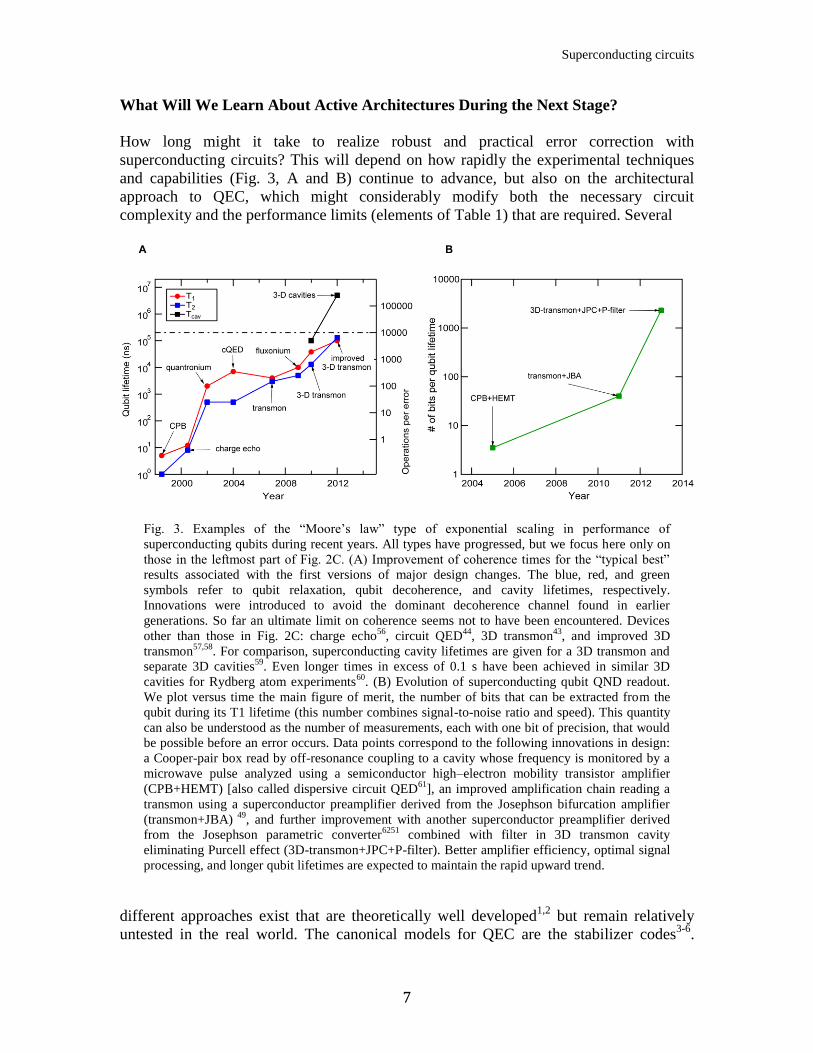
Fig. 3. Examples of the “Moore’s law” type of exponential scaling in performance of

superconducting qubits during recent years. All types have progressed, but we focus here only on

those in the leftmost part of Fig. 2C. (A) Improvement of coherence times for the “typical best”

results associated with the first versions of major design changes. The blue, red, and green

symbols refer to qubit relaxation, qubit decoherence, and cavity lifetimes, respectively.

Innovations were introduced to avoid the dominant decoherence channel found in earlier

generations. So far an ultimate limit on coherence seems not to have been encountered. Devices

other than those in Fig. 2C: charge echo56

, circuit QED44

, 3D transmon43

, and improved 3D

transmon57,58

. For comparison, superconducting cavity lifetimes are given for a 3D transmon and

separate 3D cavities59

. Even longer times in excess of 0.1 s have been achieved in similar 3D

cavities for Rydberg atom experiments60

. (B) Evolution of superconducting qubit QND readout.

We plot versus time the main figure of merit, the number of bits that can be extracted from the

qubit during its T1 lifetime (this number combines signal-to-noise ratio and speed). This quantity

can also be understood as the number of measurements, each with one bit of precision, that would

be possible before an error occurs. Data points correspond to the following innovations in design:

a Cooper-pair box read by off-resonance coupling to a cavity whose frequency is monitored by a

microwave pulse analyzed using a semiconductor high–electron mobility transistor amplifier

(CPB+HEMT) [also called dispersive circuit QED61

], an improved amplification chain reading a

transmon using a superconductor preamplifier derived from the Josephson bifurcation amplifier

(transmon+JBA) 49

, and further improvement with another superconductor preamplifier derived

from the Josephson parametric converter6251

combined with filter in 3D transmon cavity

eliminating Purcell effect (3D-transmon+JPC+P-filter). Better amplifier efficiency, optimal signal

processing, and longer qubit lifetimes are expected to maintain the rapid upward trend.

different approaches exist that are theoretically well developed1,2

but remain relatively

untested in the real world. The canonical models for QEC are the stabilizer codes3-6

.


8

Here, information is redundantly encoded in a register of entangled physical qubits

(typically, at least seven) to create a single logical qubit. Assuming that errors occur

singly, one detects them by measuring a set of certain collective properties (known as

stabilizer operators) of the qubits, and then applies appropriate additional gates to undo

the errors before the desired information is irreversibly corrupted. Thus, an experiment to

perform gates between a pair of logically encoded qubits might take a few dozen qubits,

with hundreds to thousands of individual operations. To reach a kind of “break-even”

point and perform correctly, it is required that there should be less than one error on

average during a single pass of the QEC. For a large calculation, the codes must then be

concatenated, with each qubit again being replaced by a redundant register, in a tree like

hierarchy. The so-called error correction threshold, where the resources required for this

process of expansion begin to converge, is usually estimated26

to lie in the range of error

rates of 10−3

to 10−4

, requiring values of 103 to 10

4 for the elements of Table 1. Although

these performance levels and complexity requirements might no longer be inconceivable,

they are nonetheless beyond the current state of the art, and rather daunting.

A newer approach63,64,65

is the “surface code” model of quantum computing, where a

large number of identical physical qubits are connected in a type of rectangular grid (or

“fabric”). By having specific linkages between groups of four adjacent qubits, and fast

QND measurements of their parity, the entire fabric is protected against errors. One

appeal of this strategy is that it requires a minimum number of different types of

elements, and once the development of the elementary cell is successful, the subsequent

stages of development (the fourth, fifth, and sixth stages in Fig. 1) might simply be

achieved by brute force scaling. The second advantage is that the allowable error rates are

appreciably higher, even on the order of current performance levels (a couple of percent).

However, there are two drawbacks: (i) the resource requirements (between 100 and

10,000 physical qubits per logical qubit) are perhaps even higher than in the QEC

codes65

, and (ii) the desired emergent properties of this fabric are obtained only after

hundreds, if not thousands, of qubits have been assembled and tested.

A third strategy is based on modules of nested complexity. The basic element is a small

register50

consisting of a logical memory qubit, which stores quantum information while

performing the usual kind of local error correction, and some additional communication

qubits that can interact with the memory and with other modules. By entangling the

communication qubits, one can distribute the entanglement and eventually perform a

general computation between modules. Here, the operations between the communication

bits can have relatively high error rates, or even be probabilistic and sometimes fail

entirely, provided that the communication schemes have some modest redundancy and

robustness. The adoption of techniques from cavity quantum electrodynamics (QED)66

and the advantages for routing microwave photons with transmission lines [now known

as circuit QED12,44,67

] might make on-chip versions of these schemes with

superconducting circuits an attractive alternative. Although this strategy can be viewed as

less direct and requires a variety of differing parts, its advantage is that stringent quality

tests are easier to perform at the level of each module, and hidden design flaws might be

recognized at earlier stages. Finally, once modules with sufficient performance are in

hand, they can then be programmed to realize any of the other schemes in an additional

“software layer” of error correction.


9

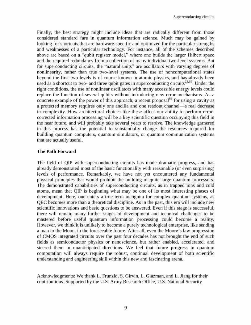
Finally, the best strategy might include ideas that are radically different from those

considered standard fare in quantum information science. Much may be gained by

looking for shortcuts that are hardware-specific and optimized for the particular strengths

and weaknesses of a particular technology. For instance, all of the schemes described

above are based on a “qubit register model,” where one builds the larger Hilbert space

and the required redundancy from a collection of many individual two-level systems. But

for superconducting circuits, the “natural units” are oscillators with varying degrees of

nonlinearity, rather than true two-level systems. The use of noncomputational states

beyond the first two levels is of course known in atomic physics, and has already been

used as a shortcut to two- and three qubit gates in superconducting circuits23,68

. Under the

right conditions, the use of nonlinear oscillators with many accessible energy levels could

replace the function of several qubits without introducing new error mechanisms. As a

concrete example of the power of this approach, a recent proposal69

for using a cavity as

a protected memory requires only one ancilla and one readout channel—a real decrease

in complexity. How architectural choices like these affect our ability to perform error-

corrected information processing will be a key scientific question occupying this field in

the near future, and will probably take several years to resolve. The knowledge garnered

in this process has the potential to substantially change the resources required for

building quantum computers, quantum simulators, or quantum communication systems

that are actually useful.

The Path Forward

The field of QIP with superconducting circuits has made dramatic progress, and has

already demonstrated most of the basic functionality with reasonable (or even surprising)

levels of performance. Remarkably, we have not yet encountered any fundamental

physical principles that would prohibit the building of quite large quantum processors.

The demonstrated capabilities of superconducting circuits, as in trapped ions and cold

atoms, mean that QIP is beginning what may be one of its most interesting phases of

development. Here, one enters a true terra incognita for complex quantum systems, as

QEC becomes more than a theoretical discipline. As in the past, this era will include new

scientific innovations and basic questions to be answered. Even if this stage is successful,

there will remain many further stages of development and technical challenges to be

mastered before useful quantum information processing could become a reality.

However, we think it is unlikely to become a purely technological enterprise, like sending

a man to the Moon, in the foreseeable future. After all, even the Moore’s law progression

of CMOS integrated circuits over the past four decades has not brought the end of such

fields as semiconductor physics or nanoscience, but rather enabled, accelerated, and

steered them in unanticipated directions. We feel that future progress in quantum

computation will always require the robust, continual development of both scientific

understanding and engineering skill within this new and fascinating arena.

Acknowledgments: We thank L. Frunzio, S. Girvin, L. Glazman, and L. Jiang for their

contributions. Supported by the U.S. Army Research Office, U.S. National Security


10

Agency Laboratory for Physical Science, U.S. Intelligence Advanced Research Projects

Activity, NSF, and Yale University.

* A version of this article has appeared as Science 339, 1169 (2013)

Requirement for scalability

Desired

capability

margins

Estimated current

capability

Demonstrated

successful performance

QI operation

Reset qubit 102- 10

4 50 Fidelity> 0.995

17

Rabi flop 102- 10

4 1000 Fidelity > 0.98

70,71

Swap to bus 102- 10

4 100 Fidelity> 0.98

72

Readout qubit 10

2- 10

4 1000 Fidelity > 0.98

51

102- 10

4 100 Efficiency > 0.4

51,25

System

Hamiltonian

Stability 106 - 10

9 ?

f/f in 1 day

< 2 × 10 -7

43

Accuracy 102- 10

4 10-100 1-10%

43

Yield >104

? ?

Complexity 10

4- 10

7 10? 1-10 qubits

73,68

Table 1. Superconducting qubits: Desired parameter margins for scalability and the corresponding

demonstrated values. Desired capability margins are numbers of successful operations or

realizations of a component before failure. For the stability of the Hamiltonian, capability is the

number of Ramsey shots that meaningfully would provide one bit of information on a parameter

(e.g., the qubit frequency) during the time when this parameter has not drifted. Estimated current

capability is expressed as number of superconducting qubits, given best decoherence times and

success probabilities. Demonstrated successful performance is given in terms of the main

performance characteristic of successful operation or Hamiltonian control (various units). A reset

qubit operation forces a qubit to take a particular state. A Rabi flop denotes a single-qubit p

rotation. A swap to bus is an operation to make a two-qubit entanglement between distant qubits.

In a readout qubit operation, the readout must be QND or must operate on an ancilla without

demolishing any memory qubit of the computer. Stability refers to the time scale during which a

Hamiltonian parameter drifts by an amount corresponding to one bit of information, or the time

scale it would take to find all such parameters in a complex system to this precision. Accuracy

can refer to the degree to which a certain Hamiltonian symmetry or property can be designed and

known in advance, the ratio by which a certain coupling can be turned on and off during

operation, or the ratio of desired to undesired couplings. Yield is the number of quantum objects

with one degree of freedom that can be made without failing or being out of specification to the

degree that the function of the whole is compromised. Complexity is the overall number of

interacting, but separately controllable, entangled degrees of freedom in a device. Question marks

indicate that more experiments are needed for a conclusive result. Values given in rightmost

column are compiled from recently published data and improve on a yearly basis.


11

References and Notes :

1 M. A. Nielsen, I. L. Chuang, Quantum Computation and

Quantum Information (Cambridge Univ. Press, Cambridge,

2000).

2 N. D. Mermin, Quantum Computer Science (Cambridge

Univ. Press, Cambridge, 2007).

3 P. W. Shor, Phys. Rev. A 52, R2493 (1995).

4 A. Steane, Proc. R. Soc. London Ser. A 452, 2551 (1996).

5 E. Knill, R. Laflamme, Phys. Rev. A 55, 900 (1997).

6 D. Gottesman, thesis, California Institute of Technology

(1997).

7 S. Lloyd, Science 273, 1073 (1996).

8 See, for example, J. I. Cirac, P. Zoller, Goals and

opportunities in quantum simulations. Nat. Phys. 8, 264

(2012) and other articles in this special issue.

9 H. J. Kimble, Nature 453, 1023 (2008).

10 Direct quantum spin simulations, such as aimed at by the

machine constructed by D-Wave Systems Inc., are outside

the scope of this article.

11 M. H. Devoret, J. M. Martinis, Quant. Inf. Proc. 3, 381

(2004).

12 R. J. Schoelkopf, S. M. Girvin, Nature 451, 664 (2008).

13 J. Clarke, F. K. Wilhelm, Nature 453, 1031 (2008).

14 J. Q. You, F. Nori, Phys. Today 58, 42 (2005).

15 D. P. DiVincenzo, Fortschr. Phys. 48, 771 (2000).

16 C. Sayrin et al., Nature 477, 73 (2011).

17 K. Geerlings et al., http://arxiv.org/abs/1211.0491 (2012).

18 R. Vijay et al., Nature 490, 77 (2012).

19 K. W. Murch et al., Phys. Rev. Lett. 109, 183602 (2012).

20 S. Diehl et al., Nat. Phys. 4, 878 (2008).

21 J. T. Barreiro et al., Nature 470, 486 (2011).

22 P. Schindler et al., Science 332, 1059 (2011).

23M. D. Reed et al., Nature 482, 382 (2012).

24 D. Ristè, C. C. Bultink, K. W. Lehnert, L. DiCarlo, Phys.

Rev. Lett. 109, 240502 (2013).

25 P. Campagne-Ibarq et al., http://arxiv.org/abs/1301.6095

(2013)

26 J. Preskill, http://arxiv.org/abs/quant-ph/9712048 (1997)

27 M. H. Devoret, in Quantum Fluctuations, S. Reynaud, E.

Giacobino, J. Zinn-Justin, Eds. (Elsevier Science,

Amsterdam, 1997).

28 V. Bouchiat, D. Vion, P. Joyez, D. Esteve, M. H. Devoret,

Phys. Scr. 1998, 165 (1998).

29 Y. Nakamura, Yu. A. Pashkin, J. S. Tsai, Nature 398, 786

(1999).

30

J. E. Mooij et al., Science 285, 1036 (1999).

31 C. H. van der Wal et al., Science 290, 773 (2000).

32 J. R. Friedman, V. Patel, W. Chen, S. K. Tolpygo, J. E.

Lukens, Nature 406, 43 (2000).

33 I. Chiorescu, Y. Nakamura, C. J. Harmans, J. E. Mooij,

Science 299, 1869 (2003).

34 J. M. Martinis, S. Nam, J. Aumentado, C. Urbina, Phys.

Rev. Lett. 89, 117901 (2002).

35 J. Martinis, Quant. Inf. Proc. 8, 81 (2009).

36 A. Cottet et al., Physica C 367, 197 (2002).

37 D. Vion et al., Science 296, 886 (2002).

38 J. Koch et al., Phys. Rev. A 76, 042319 (2007).

39 A. A. Houck et al., Phys. Rev. Lett. 101, 080502 (2008).

40 V. E. Manucharyan, J. Koch, L. I. Glazman, M. H.

Devoret, Science 326, 113 (2009).

41 M. Steffen et al., Phys. Rev. Lett. 105, 100502 (2010).

42 S. E. Nigg et al., Phys. Rev. Lett. 108, 240502 (2012).

43 H. Paik et al., Phys. Rev. Lett. 107, 240501 (2011).

44 A. Wallraff et al., Nature 431, 162 (2004).

45 A. Megrant et al., Appl. Phys. Lett. 100, 113510 (2012).

46 J. Bylander et al., Nat. Phys. 7, 565 (2011).

47 Z. Kim et al., Phys. Rev. Lett. 106, 120501 (2011).

48 A. Palacios-Laloy et al., Nat. Phys. 6, 442 (2010).

49 R. Vijay, D. H. Slichter, I. Siddiqi, Phys. Rev. Lett. 106,

110502 (2011).

50 L. M. Duan, B. B. Blinov, D. L. Moehring, C. Monroe,

Quantum Inf. Comput. 4, 165 (2004).

51 M. Hatridge et al., Science 339, 178 (2013).

52 D. Bintley et al., Proc. SPIE 8452, 845208 (2012).

53 J. Zmuidzinas, Annu. Rev. Condens. Matter Phys. 3, 169

(2012).

54 J. Jones, NMR Quantum Computation

(nmr.physics.ox.ac.uk/pdfs/lhnmrqc.pdf).

55 M. P. da Silva, O. Landon-Cardinal, D. Poulin, Phys.

Rev. Lett. 107, 210404 (2011).

56 Y. Nakamura, Y. A. Pashkin, T. Yamamoto, J. S. Tsai,

Phys. Rev. Lett. 88, 047901 (2002).

57 A. Sears et al., Phys. Rev. B 86, 180504 (2012).

58 C. Rigetti et al., Phys. Rev. B 86, 100506 (2012).

59 M. Reagor et al., http://arxiv.org/abs/1302.4408 (2013).

60 S. Kuhr et al., Appl. Phys. Lett. 90, 164101 (2007).

61 A. Wallraff et al., Phys. Rev. Lett. 95, 060501 (2005).

62 N. Bergeal et al., Nature 465, 64 (2010).


12

63

S. Bravyi, A. Yu. Kitaev, Quantum Computers Comput.

2, 43 (2001).

64 M. H. Freedman, D. A. Meyer, Found. Comput. Math. 1,

325 (2001).

65 A. G. Fowler, M. Mariantoni, J. M. Martinis, A. N.

Cleland, Phys. Rev. A 86, 032324 (2012).

66 S. Haroche, J. M. Raimond, Exploring the Quantum:

Atoms, Cavities, and Photons (Oxford Univ. Press, Oxford,

2006).

67 C. Eichler et al., Phys. Rev. Lett. 106, 220503 (2011).

68 M. Mariantoni et al., Nat. Phys. 7, 287 (2011).

69 Z. Leghtas et al., http://arxiv.org/abs/1207.0679.

70 E. Magesan et al., Phys. Rev. Lett. 109, 080505 (2012).

71 E. Lucero et al., Phys. Rev. Lett. 100, 247001 (2008).

72 J. M. Chow et al., Phys. Rev. Lett. 109, 060501 (2012).

73 A. Dewes et al., Phys Rev B 85, 140503 (2012).

Documents

Superconducting Circuits for Quantum Information: An Outlookqulab.eng.yale.edu/documents/Superconducting_Circuits... · 2020-02-08 · Superconducting circuits 1 Superconducting Circuits