Embed Size (px)
Citation preview
Superconducting Qubits and the Physics of
Josephson Junctions
John M. Martinis and Kevin Osborne
National Institute of Standards and Technology, 325 Broadway, Boulder, CO80305-3328, USA
Superconducting Qubits and the Physics of Josephson Junctions 2
1. Introduction
Josephson junctions are good candidates for the construction of quantum bits (qubits)
for a quantum computer[1]. This system is attractive because the low dissipation
inherent to superconductors make possible, in principle, long coherence times. In
addition, because complex superconducting circuits can be microfabricated using
integrated-circuit processing techniques, scaling to a large number of qubits should
be relatively straightforward. Given the initial success of several types of Josephson
qubits[2, 3, 4, 5, 6, 7, 9, 8, 10], a question naturally arises: what are the essential
components that must be tested, understood, and improved for eventual construction
of a Josephson quantum computer?
In this paper we focus on the physics of the Josephson junction because, being
nonlinear, it is the fundamental circuit element that is needed for the appearance
of usable qubit states. In contrast, linear circuit elements such as capacitors and
inductors can form low-dissipation superconducting resonators, but are unusable for
qubits because the energy-level spacings are degenerate. The nonlinearity of the
Josephson inductance breaks the degeneracy of the energy level spacings, allowing
dynamics of the system to be restricted to only the two qubit states. The Josephson
junction is a remarkable nonlinear element because it combines negligible dissipation
with extremely large nonlinearity - the change of the qubit state by only one photon in
energy can modify the junction inductance by order unity!
Most theoretical and experimental investigations with Josephson qubits assume
perfect junction behavior. Is such an assumption valid? Recent experiments by our
group indicate that coherence is limited by microwave-frequency fluctuations in the
critical current of the junction[10]. A deeper understanding of the junction physics
is thus needed so that nonideal behavior can be more readily identified, understood,
and eliminated. Although we will not discuss specific imperfections of junctions in this
paper, we want to describe a clear and precise model of the Josephson junction that can
give an intuitive understanding of the Josephson effect. This is especially needed since
textbooks do not typically derive the Josephson effect from a microscopic viewpoint.
As standard calculations use only perturbation theory, we will also need to introduce
an exact description of the Josephson effect via the mesoscopic theory of quasiparticle
bound-states.
The outline of the paper is as follows. We first describe in Sec. 2 the nonlinear
Josephson inductance. In Sec. 3 we discuss the three types of qubit circuits, and
show how these circuits use this nonlinearity in unique manners. We then give a brief
derivation of the BCS theory in Sec. 4, highlighting the appearance of the macroscopic
phase parameter. The Josephson equations are derived in Sec. 5 using standard
first and second order perturbation theory that describe quasiparticle and Cooper-pair
tunneling. An exact calculation of the Josephson effect then follows in Sec. 6 using
the quasiparticle bound-state theory. Section 7 expands upon this theory and describes
quasiparticle excitations as transitions from the ground to excited bound states from
Superconducting Qubits and the Physics of Josephson Junctions 3
φ L φ R
V I J
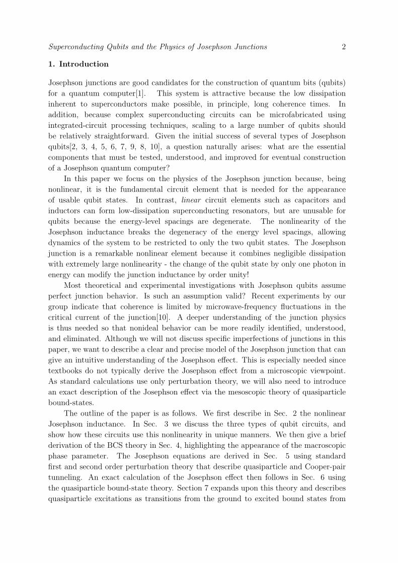
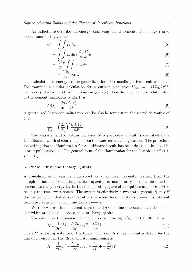
Figure 1. Schematic diagram of a Josephson junction connected to a bias voltage V .The Josephson current is given by IJ = I0 sin δ, where δ = φL − φR is the differencein the superconducting phase across the junction.
nonadiabatic changes in the bias. Although quasiparticle current is typically calculated
only for a constant DC voltage, the advantage to this approach is seen in Sec. 8,
where we qualitatively describe quasiparticle tunneling with AC voltage excitations,
as appropriate for the qubit state. This section describes how the Josephson qubit is
typically insensitive to quasiparticle damping, even to the extent that a phase qubit can
be constructed from microbridge junctions.
2. The Nonlinear Josephson Inductance
A Josephson tunnel junction is formed by separating two superconducting electrodes
with an insulator thin enough so that electrons can quantum-mechanically tunnel
through the barrier, as illustrated in Fig. 1 . The Josephson effect describes the
supercurrent IJ that flows through the junction according to the classical equations
IJ = I0 sin δ (1)
V =Φ0
2π
dδ
dt, (2)
where Φ0 = h/2e is the superconducting flux quantum, I0 is the critical-current
parameter of the junction, and δ = φL−φR and V are respectively the superconducting
phase difference and voltage across the junction. The dynamical behavior of these two
equations can be understood by first differentiating Eq. 1 and replacing dδ/dt with V
according to Eq. 2
dIJ
dt= I0 cos δ
2π
Φ0
V. (3)
With dIJ/dt proportional to V , this equation describes an inductor. By defining a
Josephson inductance LJ according to the conventional definition V = LJdIJ/dt, one
finds
LJ =Φ0
2πI0 cos δ. (4)
The 1/ cos δ term reveals that this inductance is nonlinear. It becomes large as δ → π/2,
and is negative for π/2 < δ < 3π/2. The inductance at zero bias is LJ0 = Φ0/2πI0.
Superconducting Qubits and the Physics of Josephson Junctions 4
An inductance describes an energy-conserving circuit element. The energy stored
in the junction is given by
UJ =
∫ ∫IJV dt (5)
=
∫ ∫I0 sin δ
Φ0
2π
dδ
dtdt (6)
=I0Φ0
2π
∫ ∫sin δ dδ (7)
= − I0Φ0
2πcos δ. (8)
This calculation of energy can be generalized for other nondissipative circuit elements.
For example, a similar calculation for a current bias gives Ubias = −(IΦ0/2π)δ.
Conversely, if a circuit element has an energy U(δ), then the current-phase relationship
of the element, analogous to Eq. 1, is
IJ(δ) =2π
Φ0
∂U(δ)
∂δ. (9)
A generalized Josephson inductance can be also be found from the second derivative of
U ,
1
LJ
=
(2π
Φ0
)2∂2U(δ)
∂δ2. (10)
The classical and quantum behavior of a particular circuit is described by a
Hamiltonian, which of course depends on the exact circuit configuration. The procedure
for writing down a Hamiltonian for an arbitrary circuit has been described in detail in
a prior publication[11]. The general form of the Hamiltonian for the Josephson effect is
HJ = UJ .
3. Phase, Flux, and Charge Qubits
A Josephson qubit can be understood as a nonlinear resonator formed from the
Josephson inductance and its junction capacitance. nonlinearity is crucial because the
system has many energy levels, but the operating space of the qubit must be restricted
to only the two lowest states. The system is effectively a two-state system[12] only if
the frequency ω10 that drives transitions between the qubit states 0 ←→ 1 is different
from the frequency ω21 for transitions 1 ←→ 2.
We review here three different ways that these nonlinear resonators can be made,
and which are named as phase, flux, or charge qubits.
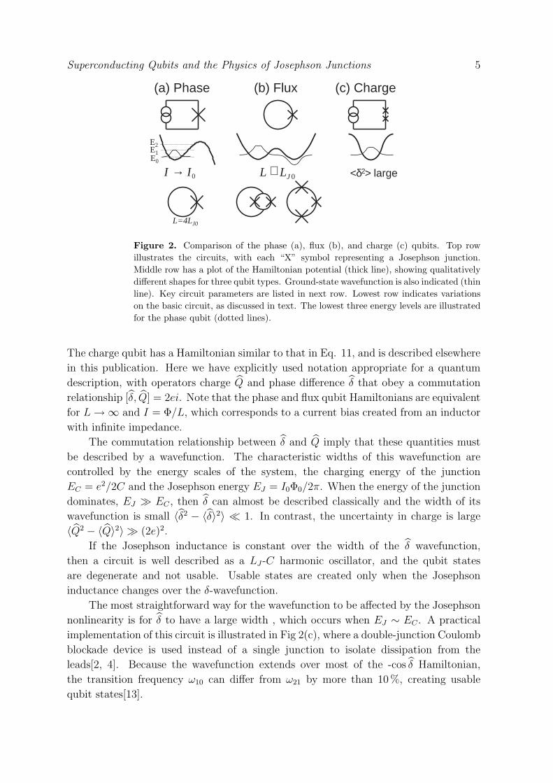
The circuit for the phase-qubit circuit is drawn in Fig. 2(a). Its Hamiltonian is
H =1
2CQ̂2 − I0Φ0
2πcos δ̂ − IΦ0
2πδ̂, (11)
where C is the capacitance of the tunnel junction. A similar circuit is drawn for the
flux-qubit circuit in Fig. 2(b), and its Hamiltonian is
H =1
2CQ̂2 − I0Φ0
2πcos δ̂ +
1
2L(Φ− Φ0
2πδ̂)2. (12)
Superconducting Qubits and the Physics of Josephson Junctions 5
(a) Phas e ( b) Flux (c) Charge
0 I I → 0 J L L ≅ <δ 2 > larg e
E 0
E 1
E 2
L=4L J0
Figure 2. Comparison of the phase (a), flux (b), and charge (c) qubits. Top rowillustrates the circuits, with each “X” symbol representing a Josephson junction.Middle row has a plot of the Hamiltonian potential (thick line), showing qualitativelydifferent shapes for three qubit types. Ground-state wavefunction is also indicated (thinline). Key circuit parameters are listed in next row. Lowest row indicates variationson the basic circuit, as discussed in text. The lowest three energy levels are illustratedfor the phase qubit (dotted lines).
The charge qubit has a Hamiltonian similar to that in Eq. 11, and is described elsewhere
in this publication. Here we have explicitly used notation appropriate for a quantum
description, with operators charge Q̂ and phase difference δ̂ that obey a commutation
relationship [δ̂, Q̂] = 2ei. Note that the phase and flux qubit Hamiltonians are equivalent
for L →∞ and I = Φ/L, which corresponds to a current bias created from an inductor
with infinite impedance.
The commutation relationship between δ̂ and Q̂ imply that these quantities must
be described by a wavefunction. The characteristic widths of this wavefunction are
controlled by the energy scales of the system, the charging energy of the junction
EC = e2/2C and the Josephson energy EJ = I0Φ0/2π. When the energy of the junction
dominates, EJ À EC , then δ̂ can almost be described classically and the width of its
wavefunction is small 〈δ̂2 − 〈δ̂〉2〉 ¿ 1. In contrast, the uncertainty in charge is large
〈Q̂2 − 〈Q̂〉2〉 À (2e)2.
If the Josephson inductance is constant over the width of the δ̂ wavefunction,
then a circuit is well described as a LJ -C harmonic oscillator, and the qubit states
are degenerate and not usable. Usable states are created only when the Josephson
inductance changes over the δ-wavefunction.
The most straightforward way for the wavefunction to be affected by the Josephson
nonlinearity is for δ̂ to have a large width , which occurs when EJ ∼ EC . A practical
implementation of this circuit is illustrated in Fig 2(c), where a double-junction Coulomb
blockade device is used instead of a single junction to isolate dissipation from the
leads[2, 4]. Because the wavefunction extends over most of the -cos δ̂ Hamiltonian,
the transition frequency ω10 can differ from ω21 by more than 10 %, creating usable
qubit states[13].
Superconducting Qubits and the Physics of Josephson Junctions 6
Josephson qubits are possible even when EJ À EC , provided that the junction
is biased to take advantage of its strong nonlinearity. A good example is the phase
qubit[6], where typically EJ ∼ 104EC , but which is biased near δ . π/2 so that the
inductance changes rapidly with δ (see Eq. 4). Under these conditions the potential can
be accurately described by a cubic potential, with the barrier height ∆U → 0 as I → I0.
Typically the bias current is adjusted so that the number of energy levels in the well is
∼ 3− 5, which causes ω10 to differ from ω21 by an acceptably large amount ∼ 5 %.
Implementing the phase qubit is challenging because a current bias is required
with large impedance. This impedance requirement can be met by biasing the junction
with flux through a superconducting loop with a large loop inductance L, as discussed
previously and drawn in Fig. 2(a). To form multiple stable flux states and a cubic
potential, the loop inductance L must be chosen such that L & 2LJ0. We have found
that a design with L ' 4.5LJ0 is a good choice since the potential well then contains
the desired cubic potential and only one flux state into which the system can tunnel,
simplifying operation.
The flux qubit is designed with L . LJ0 and biased in flux so that 〈δ̂〉 = π. Under
these conditions the Josephson inductance is negative and is almost canceled out by
L. The small net negative inductance near δ̂ = π turns positive away from this value
because of the 1/ cos δ nonlinearity, so that the final potential shape is quartic, as shown
in Fig. 2(b). An advantage of the flux qubit is a large net nonlinearity, so that ω10 can
differ from ω21 by over 100 %.
The need to closely tune L with LJ0 has inspired the invention of several variations
to the simple flux-qubit circuit, as illustrated in Fig. 2(b). One method is to use small
area junctions[7] with EJ ∼ 10EC , producing a large width in the δ̂ wavefunction and
relaxing the requirement of close tuning of L with LJ0. Another method is to make the
qubit junction a two-junction SQUID, whose critical current can then be tuned via a
second flux-bias circuit[14, 15]. Larger junctions are then permissible, with EJ ∼ 102EC
to 103EC . A third method is to fabricate the loop inductance from two or more larger
critical-current junctions[16]. These junctions are biased with phase less than π/2, and
thus act as positive inductors. The advantage to this approach is that junction inductors
are smaller than physical inductors, and fabrication imperfections in the critical currents
of the junctions tend to cancel out and make the tuning of L with LJ0 easier.
In summary, the major difference between the phase, flux, and charge qubits is the
shape of their nonlinear potentials, which are respectively cubic, quartic, and cosine. It
is impossible at this time to predict which qubit type is best because their limitations are
not precisely known, especially concerning decoherence mechanisms and their scaling.
However, some general observations can be made.
First, the flux qubit has the largest nonlinearity. This implies faster logic gates
since suppressing transitions from the qubit states 0 and 1 to state 2 requires long pulses
whose time duration scales as 1/ |ω10 − ω21|[12]. The flux qubit allows operation times
less than ∼ 1 ns, whereas for the phase qubit 10 ns is more typical. We note, however,
that this increase in speed may not be usable. Generating precise shaped pulses is much
Superconducting Qubits and the Physics of Josephson Junctions 7
more difficult on a 1 ns time scale, and transmitting these short pulses to the qubit with
high fidelity will be more problematic due to reflections or other imperfections in the
microwave lines.
Second, the choice between large and small junctions involve tradeoffs. Large
junctions (EJ À EC) require precise tuning of parameters (L/LJ0 for the flux qubit) or
biases (I/I0 for the phase qubit) to produce the required nonlinearity. Small junctions
(EJ ∼ EC) do not require such careful tuning, but become sensitive to 1/f charge
fluctuations because EC has relatively larger magnitude.
Along these lines, the coherence of qubits have been compared considering the effect
of low-frequency 1/f fluctuations of the critical current[17]. These calculations include
the known scaling of the fluctuations with junction size and the sensitivity to parameter
fluctuations. It is interesting that the calculated coherence times for the flux and phase
qubits are similar. With parameters choosen to give an oscillation frequency of ∼ 1 GHz
for the flux qubit and ∼ 10 GHz for the phase qubit, the number of coherent logic-gate
operations is even approximately the same.
4. BCS Theory and the Superconducting State
A more complete understanding of the Josephson effect will require a derivation of Eqs.
1 and 2. In order to calculate this microscopically, we will first review the BCS theory of
superconductivity [18] using a “pair spin” derivation that we believe is more physically
clear than the standard energy-variational method. Although the calculation follows
closely that of Anderson[19] and Kittel[20], we have expanded it slightly to describe
the physics of the superconducting phase, as appropriate for understanding Josephson
qubits.
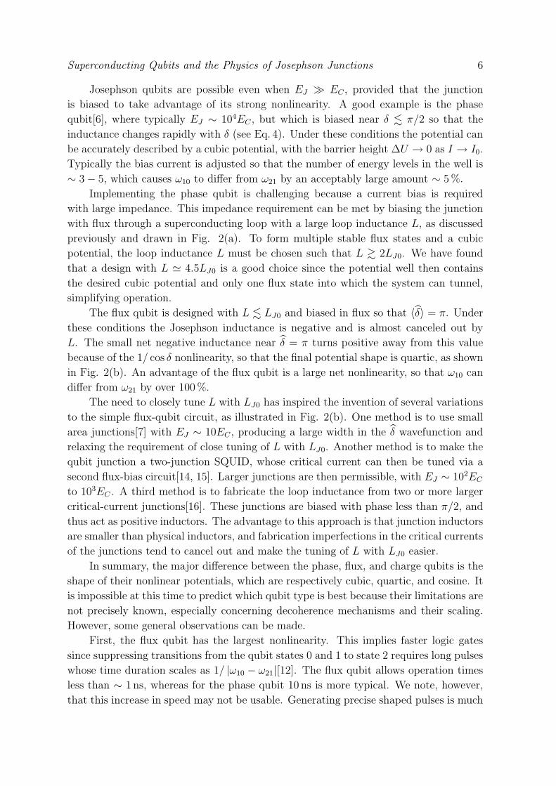
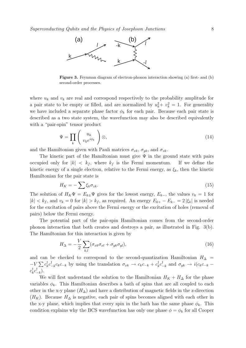
In a conventional superconductor, the attractive interaction that produces
superconductivity comes from the scattering of electrons and phonons. As illustrated in
Fig. 3(a), to first order the phonon interaction scatters an electron from one momentum
state to another. When taken to second order (Fig. 3(b)), the scattering of a virtual
phonon produces a net attractive interaction between two pairs of electrons. The first-
order phonon scattering rates are generally small, not because of the phonon matrix
element, but because phase space is small for the final electron state. This implies that
the energy of the second order interaction can be significant if there are large phase-space
factors.
The electron pairs have the largest net interaction if every pair is allowed by phase
space factors to interact with every other pair. This is explicitly created in the BCS
wavefunction by including only pair states (Cooper pairs) with zero net momentum.
Under this assumption and using a second quantized notation where c†k is the usual
creation operator for an electron state of wavevector k, the most general form for the
electronic wavefunction is
Ψ =∏
k
(uk + vkeiφkc†kc
†−k) |0〉 , (13)
Superconducting Qubits and the Physics of Josephson Junctions 8
(a ) ( b)
k
l
k
-k l
-l
Figure 3. Feynman diagram of electron-phonon interaction showing (a) first- and (b)second-order processes.
where uk and vk are real and correspond respectively to the probability amplitude for
a pair state to be empty or filled, and are normalized by u2k+ v2
k = 1. For generality
we have included a separate phase factor φk for each pair. Because each pair state is
described as a two state system, the wavefunction may also be described equivalently
with a “pair-spin” tensor product
Ψ =∏
k
(uk
vkeiφk
)⊗, (14)
and the Hamiltonian given with Pauli matrices σxk, σyk, and σzk.
The kinetic part of the Hamiltonian must give Ψ in the ground state with pairs
occupied only for |k| < kf , where kf is the Fermi momentum. If we define the
kinetic energy of a single electron, relative to the Fermi energy, as ξk, then the kinetic
Hamiltonian for the pair state is
HK = −∑
ξkσzk. (15)
The solution of HKΨ = Ek±Ψ gives for the lowest energy, Ek−, the values vk = 1 for
|k| < kf , and vk = 0 for |k| > kf , as required. An energy Ek+ − Ek− = 2 |ξk| is needed
for the excitation of pairs above the Fermi energy or the excitation of holes (removal of
pairs) below the Fermi energy.
The potential part of the pair-spin Hamiltonian comes from the second-order
phonon interaction that both creates and destroys a pair, as illustrated in Fig. 3(b).
The Hamiltonian for this interaction is given by
H∆ = −V
2
∑
k,l
(σxkσxl + σykσyl), (16)
and can be checked to correspond to the second-quantization Hamiltonian H∆ =
−V∑
c†kc†−kckc−k by using the translation σxk → ckc−k + c†kc
†−k and σyk → i(ckc−k −
c†kc†−k).
We will first understand the solution to the Hamiltonian HK + H∆ for the phase
variables φk. This Hamiltonian describes a bath of spins that are all coupled to each
other in the x-y plane (H∆) and have a distribution of magnetic fields in the z-direction
(HK). Because H∆ is negative, each pair of spins becomes aligned with each other in
the x-y plane, which implies that every spin in the bath has the same phase φk. This
condition explains why the BCS wavefunction has only one phase φ = φk for all Cooper
Superconducting Qubits and the Physics of Josephson Junctions 9
pairs[21]. Because there is no preferred direction in the x-y plane, the solution to the
Hamiltonian is degenerate with respect to φ and the wavefunction for φ is separable
from the rest of the wavefunction. Normally, this means that φ can be treated as a
classical variable, as is done for the conventional understanding of superconductivity
and the Josephson effects. For Josephson qubits, where φ must be treated quantum
mechanically, then the behavior of φ is described by an external-circuit Hamiltonian, as
was done in Sec. 3.
For a superconducting circuit, where one electrode is biased with a voltage V ,
the voltage can be accounted for with a gauge transformation on each electron state
c†k → ei(e/~)R
V dtc†k. The change in the superconducting state is thus given by
Ψ →∏
k
(uk + vkeiφei(e/~)
RV dtc†ke
i(e/~)R
V dtc†−k) |0〉 (17)
=∏
k
(uk + vkei[φ+i(2e/~)
RV dt]c†kc
†−k) |0〉 . (18)
The change in φ can be written equivalently as
dφ
dt=
2eV
~, (19)
which leads to the AC Josephson effect.
The solution for uk and vk proceeds using the standard method of mean-field theory,
with
〈H∆〉 = − V
2
∑
k,l
(σxk 〈σxl〉+ σyk 〈σyl〉), (20)
〈σxl〉 =(ul, vle
−iφ) · σx ·
(ul
vleiφ
)(21)
= 2ulvl cos φ, (22)
〈σyl〉 = 2ulvl sin φ. (23)
Using the standard definition of the gap potential, one finds
∆ = V∑
l
ulvl, (24)
H = HK + 〈H∆〉 (25)
= −∑
k
(σxk, σyk, σzk) · (∆ cos φ, ∆ sin φ, ξk). (26)
This Hamiltonian is equivalent to a spin 1/2 particle in a magnetic field, and its
solution is well known. The energy eigenvalues of HΨ = Ek±Ψ are given by the total
length of the field vector,
Ek± = ±(∆2 + ξ2k)
1/2, (27)
and the directions of the Bloch vectors describing the Ek+ and Ek− eigenstates are
respectively parallel and antiparallel to the direction of the field vector, as illustrated in
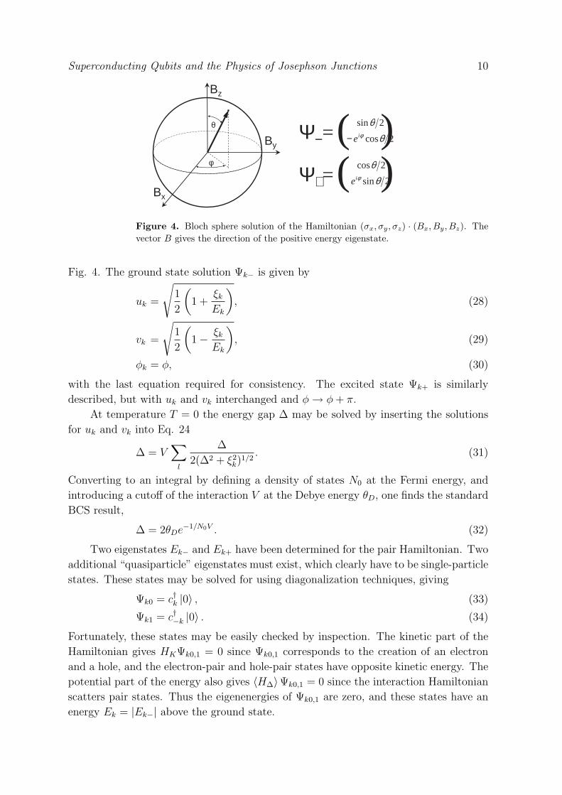
Superconducting Qubits and the Physics of Josephson Junctions 10
θ
φ
B x
B y
B z
( ) Ψ + = 2 co s θ 2 si n θ φ i e
( ) Ψ − = 2 si n θ
2 co s θ φ i e −
Figure 4. Bloch sphere solution of the Hamiltonian (σx, σy, σz) · (Bx, By, Bz). Thevector B gives the direction of the positive energy eigenstate.
Fig. 4. The ground state solution Ψk− is given by
uk =
√1
2
(1 +
ξk
Ek
), (28)
vk =
√1
2
(1− ξk
Ek
), (29)
φk = φ, (30)
with the last equation required for consistency. The excited state Ψk+ is similarly
described, but with uk and vk interchanged and φ → φ + π.
At temperature T = 0 the energy gap ∆ may be solved by inserting the solutions
for uk and vk into Eq. 24
∆ = V∑
l
∆
2(∆2 + ξ2k)
1/2. (31)
Converting to an integral by defining a density of states N0 at the Fermi energy, and
introducing a cutoff of the interaction V at the Debye energy θD, one finds the standard
BCS result,
∆ = 2θDe−1/N0V . (32)
Two eigenstates Ek− and Ek+ have been determined for the pair Hamiltonian. Two
additional “quasiparticle” eigenstates must exist, which clearly have to be single-particle
states. These states may be solved for using diagonalization techniques, giving
Ψk0 = c†k |0〉 , (33)
Ψk1 = c†−k |0〉 . (34)
Fortunately, these states may be easily checked by inspection. The kinetic part of the
Hamiltonian gives HKΨk0,1 = 0 since Ψk0,1 corresponds to the creation of an electron
and a hole, and the electron-pair and hole-pair states have opposite kinetic energy. The
potential part of the energy also gives 〈H∆〉Ψk0,1 = 0 since the interaction Hamiltonian
scatters pair states. Thus the eigenenergies of Ψk0,1 are zero, and these states have an
energy Ek = |Ek−| above the ground state.
Superconducting Qubits and the Physics of Josephson Junctions 11
0 ) ( + −
+ − + = Ψ k k
i k k k c c e v u φ
0 0 0 +
− + = Ψ = Ψ k k k k c γ
0 ) ( + −
+ + − = Ψ k k
i k k k c c e u v φ
+ 0 k γ +
1 k γ
+ 1 k
i e γ φ + − 0 k i e γ φ
k E
k E
0 1 1 + − −
+ = Ψ = Ψ k k k k c γ
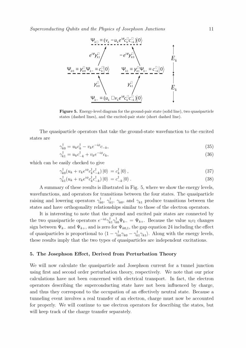
Figure 5. Energy-level diagram for the ground-pair state (solid line), two quasiparticlestates (dashed lines), and the excited-pair state (short dashed line).
The quasiparticle operators that take the ground-state wavefunction to the excited
states are
γ†k0 = ukc†k − vke
−iφc−k, (35)
γ†k1 = ukc†−k + vke
−iφck, (36)
which can be easily checked to give
γ†k0(uk + vkeiφc†kc
†−k) |0〉 = c†k |0〉 , (37)
γ†k1(uk + vkeiφc†kc
†−k) |0〉 = c†−k |0〉 . (38)
A summary of these results is illustrated in Fig. 5, where we show the energy levels,
wavefunctions, and operators for transitions between the four states. The quasiparticle
raising and lowering operators γ†k0, γ†k1, γk0, and γk1 produce transitions between the
states and have orthogonality relationships similar to those of the electron operators.
It is interesting to note that the ground and excited pair states are connected by
the two quasiparticle operators e−iφγ†k1γ†k0Ψk− = Ψk+. Because the value ulvl changes
sign between Ψk− and Ψk+, and is zero for Ψk0,1, the gap equation 24 including the effect
of quasiparticles is proportional to 〈1− γ†k0γk0 − γ†k1γk1〉. Along with the energy levels,
these results imply that the two types of quasiparticles are independent excitations.
5. The Josephson Effect, Derived from Perturbation Theory
We will now calculate the quasiparticle and Josephson current for a tunnel junction
using first and second order perturbation theory, respectively. We note that our prior
calculations have not been concerned with electrical transport. In fact, the electron
operators describing the superconducting state have not been influenced by charge,
and thus they correspond to the occupation of an effectively neutral state. Because a
tunneling event involves a real transfer of an electron, charge must now be accounted
for properly. We will continue to use electron operators for describing the states, but
will keep track of the charge transfer separately.
Superconducting Qubits and the Physics of Josephson Junctions 12
When an electron tunnels through the barrier, an electron and hole state is created
on the opposite (left and right) side of the barrier. The tunneling Hamiltonian for this
process can be written as
HT =−→H T+ +
−→H T− +
←−H T+ +
←−H T− (39)
=∑L,R
(tLRcLc†R + t−L−Rc−Lc†−R + t∗LRc†LcR + t∗−L−Rc†−Lc−R
), (40)
where tLR is the tunneling matrix element, and the L and R indices refer respectively to
momentum states k on the left and right superconductor. The first two terms−→H T+ and−→
H T− correspond to the tunneling of one electron from left to the right, whereas←−H T+
and←−H T− are for tunneling to the left. The Hamiltonian is explicitly broken up into−→
H T+ and−→H T− to account for the different electron operators c†k and c†−k for positive
and negative momentum.
The electron operators must first be expressed in terms of the quasiparticle oper-
ators γ because these produce transitions between eigenstates of the superconducting
Hamiltonian. Equations 35, 36, and their adjoints are used to solve for the four electron
operators
ck = ukγk0 + vkeiφγ†k1 c−k = ukγk1 − vke
iφγ†k0
c†k = ukγ†k0 + vke
−iφγk1 c†−k = ukγ†k1 − vke
−iφγk0.(41)
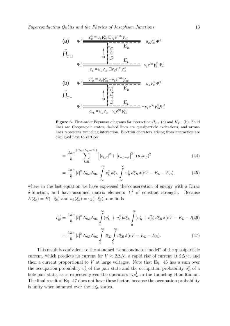
Substituting Eqs. 41 into 40, one sees that all four terms of the Hamiltonian
have operators γ† that produce quasiparticles. We calculate here to first order the
quasiparticle current from L to R given by−→H T+ +
−→H T−. The Feynman diagrams
(a) and (b) in Fig. 6 respectively describe the tunneling Hamiltonian for the−→H T+
and−→H T− terms. In this diagram a solid line represents a Cooper pair state in the
ground state, whereas a quasiparticle state is given by a dashed line. Only one pair
participates in the tunneling interaction, so only one of the three solid lines is converted
to a dashed line. The line of triangles represents the tunneling event and is labeled
with its corresponding HT Hamiltonian, with the direction of the triangles indicating
the direction of the electron tunneling. The c†k operators, acting on the L or R lead,
is rewritten in terms of the γ operators and placed above or below the vertices. Since
only γ† operators give a nonzero term when acting on the ground state, the effect of
the interaction is to produce final states ΨL,Rf with total energy ER + EL, and with
amplitudes given at the right of the figure.
The two final states in Fig 6(a) and (b) are orthogonal, as well as states involving
different values of L and R. The total current is calculated as an incoherent sum over
all possible final quasiparticle states, under the condition that the total quasiparticle
energy for the final state is equal to the energy gained by the tunneling of the electron
ER + EL = eV. (42)
The total current from L to R is given by e multiplied by the transition rate
−→Iqp = e
2π
~
(ER+EL=eV )∑L,R
∣∣∣⟨ΨL
f
∣∣ ⟨ΨR
f
∣∣−→H T+ +−→H T−
∣∣ΨR−⟩ ∣∣ΨL
−⟩∣∣∣
2
(43)
Superconducting Qubits and the Physics of Josephson Junctions 13
R
L
LR
c
c t
+
e
1 0 R i
k R R R R e v u c γ γ φ − + + + =
+ + = 1 0 L i
L L L L L e v u c γ γ φ
L E
R E
L − Ψ L
L i
L L e v −
+ Ψ 1 γ φ
R R R u − + Ψ 0 γ R
− Ψ
R
L
R
L
c c
t − +
− −
−
e
0 1 R i
k R R R R e v u c γ γ φ − + +
− − =
+ − − = 0 1 L
i L L L L
L e v u c γ γ φ
L E
R E
L − Ψ L
L i
L L e v −
+ Ψ − 0 γ φ
R R R u − + Ψ 1 γ R
− Ψ
(a )
(b )
→
+ T H
→
− T H
Figure 6. First-order Feynman diagrams for interaction HT+ (a) and HT− (b). Solidlines are Cooper-pair states, dashed lines are quasiparticle excitations, and arrow-lines represents tunneling interaction. Electron operators arising from interaction aredisplayed next to vertices.
=2πe
~
(ER+EL=eV )∑L,R
[|tLR|2 +
∣∣t−L−R
∣∣2](uRvL)2 (44)
=4πe
~|t|2 N0RN0L
∞∫
−∞
v2L dξL
∞∫
−∞
u2R dξR δ(eV − EL − ER), (45)
where in the last equation we have expressed the conservation of energy with a Dirac
δ-function, and have assumed matrix elements |t|2 of constant strength. Because
E(ξk) = E(−ξk) and uk(ξk) = vk(−ξk), one finds
−→Iqp =
4πe
~|t|2 N0RN0L
∞∫
0
(v2L + u2
L)dξL
∞∫
0
(u2R + v2
R) dξR δ(eV − EL − ER)(46)
=4πe
~|t|2 N0RN0L
∞∫
0
dξL
∞∫
0
dξR δ(eV − EL − ER). (47)
This result is equivalent to the standard “semiconductor model” of the quasiparticle
current, which predicts no current for V < 2∆/e, a rapid rise of current at 2∆/e, and
then a current proportional to V at large voltages. Note that Eq. 45 has a sum over
the occupation probability v2L of the pair state and the occupation probability u2
R of a
hole-pair state, as is expected given the operators cLc†R in the tunneling Hamiltonian.
The final result of Eq. 47 does not have these factors because the occupation probability
is unity when summed over the ±ξk states.
Superconducting Qubits and the Physics of Josephson Junctions 14
R
L
R
L
c c
t − +
− −
−
e e
+ 0 R R u γ
+ 1 L
i L
L e v γ φ
0 R i
R R e v γ φ − −
1 L L u γ L E
R E
L − Ψ
R − Ψ
L − Ψ
R − Ψ (a )
(b )
→
+ T H
→
− T H
→
− T H
R
L
LR
c
c t
+
→
+ T H
R
L
R
L
c c
t − +
− −
−
e e
+ 1 R R u γ
+ − 0 L i
L L e v γ φ
1 R i
R R e v γ φ −
0 L L u γ L E
R E
L − Ψ
R − Ψ
L − Ψ
R − Ψ
R
L
LR
c
c t
+
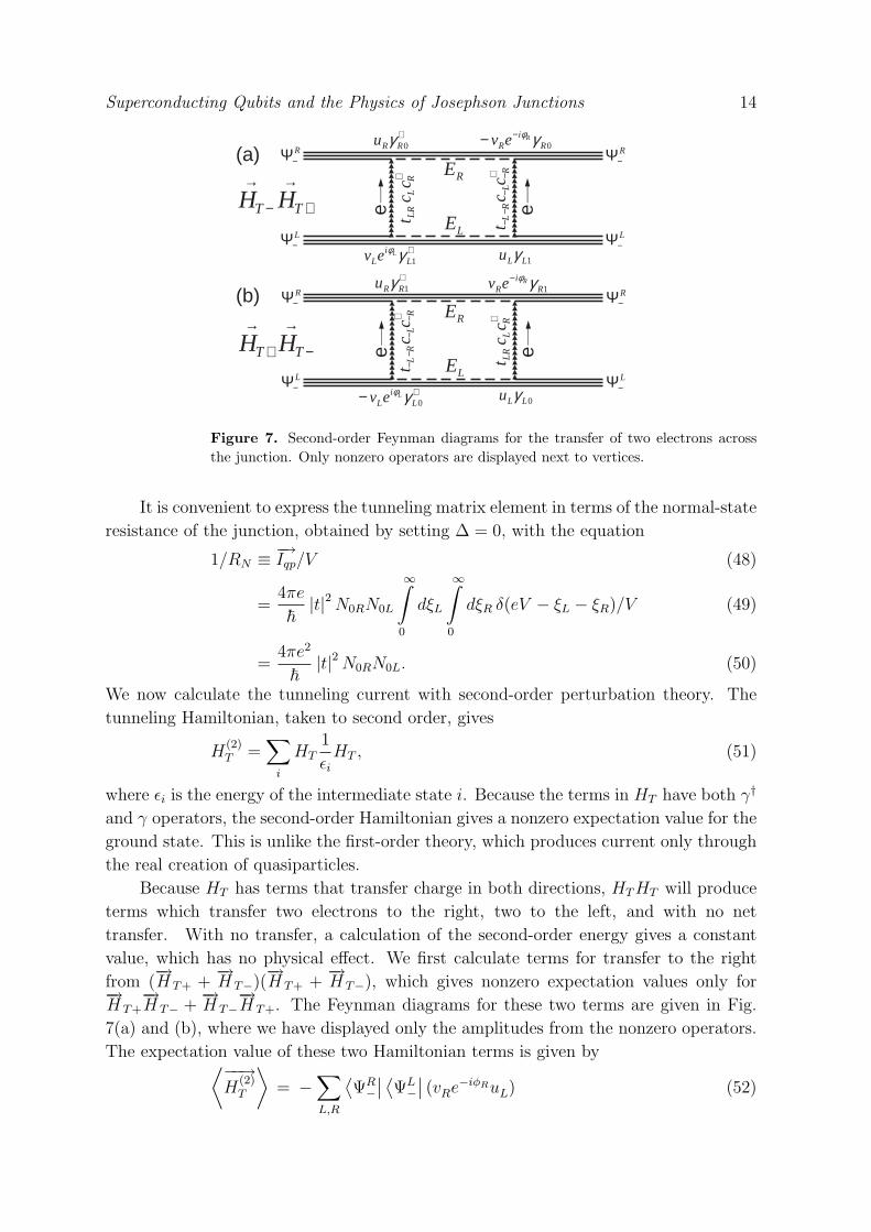
Figure 7. Second-order Feynman diagrams for the transfer of two electrons acrossthe junction. Only nonzero operators are displayed next to vertices.
It is convenient to express the tunneling matrix element in terms of the normal-state
resistance of the junction, obtained by setting ∆ = 0, with the equation
1/RN ≡ −→Iqp/V (48)
=4πe
~|t|2 N0RN0L
∞∫
0
dξL
∞∫
0
dξR δ(eV − ξL − ξR)/V (49)
=4πe2
~|t|2 N0RN0L. (50)
We now calculate the tunneling current with second-order perturbation theory. The
tunneling Hamiltonian, taken to second order, gives
H(2)T =
∑i
HT1
εi
HT , (51)
where εi is the energy of the intermediate state i. Because the terms in HT have both γ†
and γ operators, the second-order Hamiltonian gives a nonzero expectation value for the
ground state. This is unlike the first-order theory, which produces current only through
the real creation of quasiparticles.
Because HT has terms that transfer charge in both directions, HT HT will produce
terms which transfer two electrons to the right, two to the left, and with no net
transfer. With no transfer, a calculation of the second-order energy gives a constant
value, which has no physical effect. We first calculate terms for transfer to the right
from (−→H T+ +
−→H T−)(
−→H T+ +
−→H T−), which gives nonzero expectation values only for−→
H T+−→H T− +
−→H T−
−→H T+. The Feynman diagrams for these two terms are given in Fig.
7(a) and (b), where we have displayed only the amplitudes from the nonzero operators.
The expectation value of these two Hamiltonian terms is given by⟨−−→H
(2)T
⟩= −
∑L,R
⟨ΨR−∣∣ ⟨
ΨL−∣∣ (vRe−iφRuL) (52)
Superconducting Qubits and the Physics of Josephson Junctions 15
× γR0γL1γ†R0γ
†L1tLRt−L−R + γR1γL0γ
†R1γ
†L0t−L−RtLR
ER + EL
(53)
× (uRvLeiφL)∣∣ΨL
−⟩ ∣∣ΨR
−⟩
(54)
= − 2 |t|2 ei(φL−φR)∑L,R
(vRuR)(uLvL)1
ER + EL
(55)
= − 2 |t|2 eiδN0RN0L
∞∫
−∞
dξR
∞∫
−∞
dξL∆
ER
∆
EL
1
ER + EL
(56)
= − ~∆2πe2RN
eiδ
∞∫
−∞
dθR
∞∫
−∞
dθL1
cosh θR + cosh θL
(57)
= − ~∆2πe2RN
eiδ(π
2
)2
, (58)
where we have used t∗LR = t−L−R and assumed the same gap ∆ for both superconductors.
A similar calculation for transfer to the left gives the complex conjugate of Eq. 58. The
sum of these two energies gives the Josephson energy UJ , and using Eq. 9, the Josephson
current IJ ,
UJ = − 1
8
RK
RN
∆ cos δ, (59)
IJ =π
2
∆
eRN
sin δ, (60)
where RK = h/e2 is the resistance quantum. Equation 60 is the standard Ambegaokar-
Baratoff formula[22] for the Josephson current at zero temperature.
The Josephson current is a dissipationless current because it arises from a new
ground state of the two superconductors produced by the tunneling interaction. This
behavior is in contrast with quasiparticle tunneling, which is dissipative because it
produces excitations. It is perhaps surprising that a new ground state can produce
charge transfer through the junction. This is possible only because the virtual
quasiparticle excitations are both electrons and holes: the electron-part tunnels first
through the junction, then the hole-part tunnels back. Only states of energy ∆ around
the Fermi energy are both electron- and hole-like, as weighted by the (vRuR)(uLvL) term
in the integral.
The form of the Josephson Hamiltonian can be understood readily by noting that
the second-order Hamiltonian,−→H T+
−→H T− ∼ |t|2
∑L,R
cLc−Lc†Rc†−R (61)
=|t|22
∑L,R
(σxLσxR + σyLσyR), (62)
corresponds to the pair-scattering Hamiltonian of Eq. 16. Comparing with the gap-
equation solution, one expects UJ ∼ |t|2 ∆ cos δ, where the cos δ term arises from the
spin-spin interaction in the x-y plane.
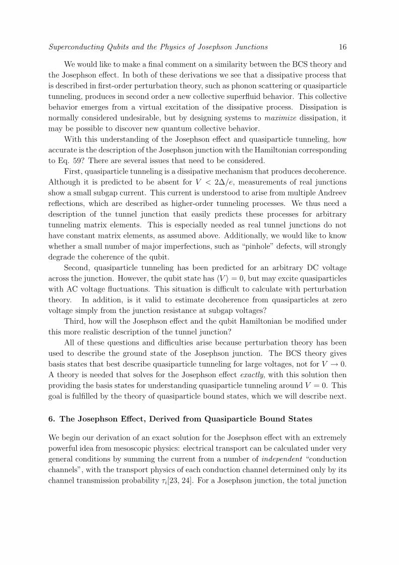
Superconducting Qubits and the Physics of Josephson Junctions 16
We would like to make a final comment on a similarity between the BCS theory and
the Josephson effect. In both of these derivations we see that a dissipative process that
is described in first-order perturbation theory, such as phonon scattering or quasiparticle
tunneling, produces in second order a new collective superfluid behavior. This collective
behavior emerges from a virtual excitation of the dissipative process. Dissipation is
normally considered undesirable, but by designing systems to maximize dissipation, it
may be possible to discover new quantum collective behavior.
With this understanding of the Josephson effect and quasiparticle tunneling, how
accurate is the description of the Josephson junction with the Hamiltonian corresponding
to Eq. 59? There are several issues that need to be considered.
First, quasiparticle tunneling is a dissipative mechanism that produces decoherence.
Although it is predicted to be absent for V < 2∆/e, measurements of real junctions
show a small subgap current. This current is understood to arise from multiple Andreev
reflections, which are described as higher-order tunneling processes. We thus need a
description of the tunnel junction that easily predicts these processes for arbitrary
tunneling matrix elements. This is especially needed as real tunnel junctions do not
have constant matrix elements, as assumed above. Additionally, we would like to know
whether a small number of major imperfections, such as “pinhole” defects, will strongly
degrade the coherence of the qubit.
Second, quasiparticle tunneling has been predicted for an arbitrary DC voltage
across the junction. However, the qubit state has 〈V 〉 = 0, but may excite quasiparticles
with AC voltage fluctuations. This situation is difficult to calculate with perturbation
theory. In addition, is it valid to estimate decoherence from quasiparticles at zero
voltage simply from the junction resistance at subgap voltages?
Third, how will the Josephson effect and the qubit Hamiltonian be modified under
this more realistic description of the tunnel junction?
All of these questions and difficulties arise because perturbation theory has been
used to describe the ground state of the Josephson junction. The BCS theory gives
basis states that best describe quasiparticle tunneling for large voltages, not for V → 0.
A theory is needed that solves for the Josephson effect exactly, with this solution then
providing the basis states for understanding quasiparticle tunneling around V = 0. This
goal is fulfilled by the theory of quasiparticle bound states, which we will describe next.
6. The Josephson Effect, Derived from Quasiparticle Bound States
We begin our derivation of an exact solution for the Josephson effect with an extremely
powerful idea from mesoscopic physics: electrical transport can be calculated under very
general conditions by summing the current from a number of independent “conduction
channels”, with the transport physics of each conduction channel determined only by its
channel transmission probability τi[23, 24]. For a Josephson junction, the total junction
Superconducting Qubits and the Physics of Josephson Junctions 17
(a ) ( b) ) ( 0 x V δ ik x e ik x e −
ik x e
) ( 0 x V δ
x k b e −
x x
x k b e
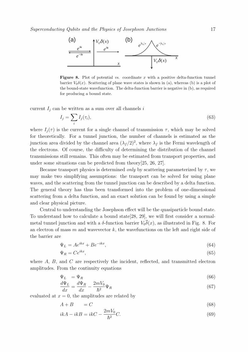
Figure 8. Plot of potential vs. coordinate x with a positive delta-function tunnelbarrier V0δ(x). Scattering of plane wave states is shown in (a), whereas (b) is a plot ofthe bound-state wavefunction. The delta-function barrier is negative in (b), as requiredfor producing a bound state.
current Ij can be written as a sum over all channels i
Ij =∑
i
Ij(τi), (63)
where Ij(τ) is the current for a single channel of transmission τ , which may be solved
for theoretically. For a tunnel junction, the number of channels is estimated as the
junction area divided by the channel area (λf/2)2, where λf is the Fermi wavelength of
the electrons. Of course, the difficulty of determining the distribution of the channel
transmissions still remains. This often may be estimated from transport properties, and
under some situations can be predicted from theory[25, 26, 27].
Because transport physics is determined only by scattering parameterized by τ , we
may make two simplifying assumptions: the transport can be solved for using plane
waves, and the scattering from the tunnel junction can be described by a delta function.
The general theory has thus been transformed into the problem of one-dimensional
scattering from a delta function, and an exact solution can be found by using a simple
and clear physical picture.
Central to understanding the Josephson effect will be the quasiparticle bound state.
To understand how to calculate a bound state[28, 29], we will first consider a normal-
metal tunnel junction and with a δ-function barrier V0δ(x), as illustrated in Fig. 8. For
an electron of mass m and wavevector k, the wavefunctions on the left and right side of
the barrier are
ΨL = Aeikx + Be−ikx, (64)
ΨR = Ceikx, (65)
where A, B, and C are respectively the incident, reflected, and transmitted electron
amplitudes. From the continuity equations
ΨL = ΨR (66)
dΨL
dx=
dΨR
dx− 2mV0
~2ΨR (67)
evaluated at x = 0, the amplitudes are related by
A + B = C (68)
ikA− ikB = ikC − 2mV0
~2C. (69)
Superconducting Qubits and the Physics of Josephson Junctions 18
�
fk+
�E�u
fk�
00 �
�E+
�E�
�
� � +�ABC
D E( )�v
�u( )�v� �v( )�u�
( )�v
�u
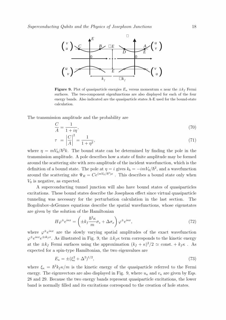
Figure 9. Plot of quasiparticle energies Eκ versus momentum κ near the ±kf Fermisurfaces. The two-component eigenfunctions are also displayed for each of the fourenergy bands. Also indicated are the quasiparticle states A-E used for the bound-statecalculation.
The transmission amplitude and the probability are
C
A=
1
1 + iη, (70)
τ =
∣∣∣∣C
A
∣∣∣∣2
=1
1 + η2, (71)
where η = mV0/~2k. The bound state can be determined by finding the pole in the
transmission amplitude. A pole describes how a state of finite amplitude may be formed
around the scattering site with zero amplitude of the incident wavefunction, which is the
definition of a bound state. The pole at η = i gives kb = −imV0/~2, and a wavefunction
around the scattering site ΨR = Ce(mV0/~2)x . This describes a bound state only when
V0 is negative, as expected.
A superconducting tunnel junction will also have bound states of quasiparticles
excitations. These bound states describe the Josephson effect since virtual quasiparticle
tunneling was necessary for the perturbation calculation in the last section. The
Bogoliubov-deGennes equations describe the spatial wavefunctions, whose eigenstates
are given by the solution of the Hamiltonian
Hϕ±eiκx =
(±kf
~2κ
mσz + ∆σx
)ϕ±eiκx, (72)
where ϕ±eiκx are the slowly varying spatial amplitudes of the exact wavefunction
ϕ±eiκxe±ikf x. As illustrated in Fig. 9, the ±kfκ term corresponds to the kinetic energy
at the ±kf Fermi surfaces using the approximation (kf + κ)2/2 ' const. + kfκ . As
expected for a spin-type Hamiltonian, the two eigenvalues are
Eκ = ±(ξ2κ + ∆2)1/2, (73)
where ξκ = ~2kfκ/m is the kinetic energy of the quasiparticle referred to the Fermi
energy. The eigenvectors are also displayed in Fig. 9, where uκ and vκ are given by Eqs.
28 and 29. Because the two energy bands represent quasiparticle excitations, the lower
band is normally filled and its excitations correspond to the creation of hole states.
Superconducting Qubits and the Physics of Josephson Junctions 19
We can solve for the quasiparticle bound states by first writing down the
scattering wavefunctions in the left and right superconducting electrodes. An incoming
quasiparticle state, point A in Fig. 9, is reflected off the tunnel barrier to states B and
C and is transmitted to states D and E [30]. The wavefunctions are then given by
ΨL = A
(u
veiφL
)eiκx + B
(v
ueiφL
)eiκx + C
(u
veiφL
)e−iκx (74)
ΨR = D
(v
ueiφR
)e−iκx + E
(u
veiφR
)eiκx, (75)
where we have used the relations v ≡ vκ = u−κ and u ≡ uκ = v−κ, and we have included
the phases φL and φR of the two states. The continuity conditions Eqs. 66 and 67,
solved for both the components of the spin wavefunction, gives the matrix equation
A
u
v
u
v
=
−v −u v u
−u −v ue−iδ ve−iδ
−v u −v(1− i2η) u(1 + i2η)
−u v −ue−iδ(1− i2η) ve−iδ(1 + i2η)
B
C
D
E
.(76)
The scattering amplitudes for B-E have poles given by the solution of
(u4 + v4)(1 + η2)− 2(uv)2(η2 + cos δ) = 0. (77)
Using the relations u2 + v2 = 1, EJ = Ek = ∆/2uv, and τ = 1/(1 + η2), the energies of
the quasiparticle bound states are
EJ± = ±∆[1− τ sin2(δ/2)]1/2. (78)
Because these two states have energies less than the gap energy ∆, they are energetically
“bound” to the junction and thus have wavefunctions that are localized around the
junction.
The dependence of the quasiparticle bound-state energies on junction phase is
plotted in Fig. 10 for several values of τ . The ground state is normally filled, similar
to the filling of quasiparticle states of negative energy. The energy EJ− corresponds to
the Josephson energy, as can be checked in the limit τ → 0 to give
EJ− ' −∆ +∆τ
4− ∆τ
4cos δ. (79)
This result is equivalent to Eq. 59 after noting that the normal-state conductance of a
single channel is 1/RN = 2τ/RK .
The current of each bound state is given by the derivative of its energy
IJ± =2π
Φ0
∂EJ±∂δ
, (80)
in accord with Eq. 9. Since the curvature of the upper band is opposite to that
of the lower band, the currents of the two bands have opposite sign IJ+ = −IJ−.
For level populations of the two states given by f±, the average Josephson current is
〈IJ〉 = IJ−(f− − f+). For a thermal population, f± are given by Fermi distributions,
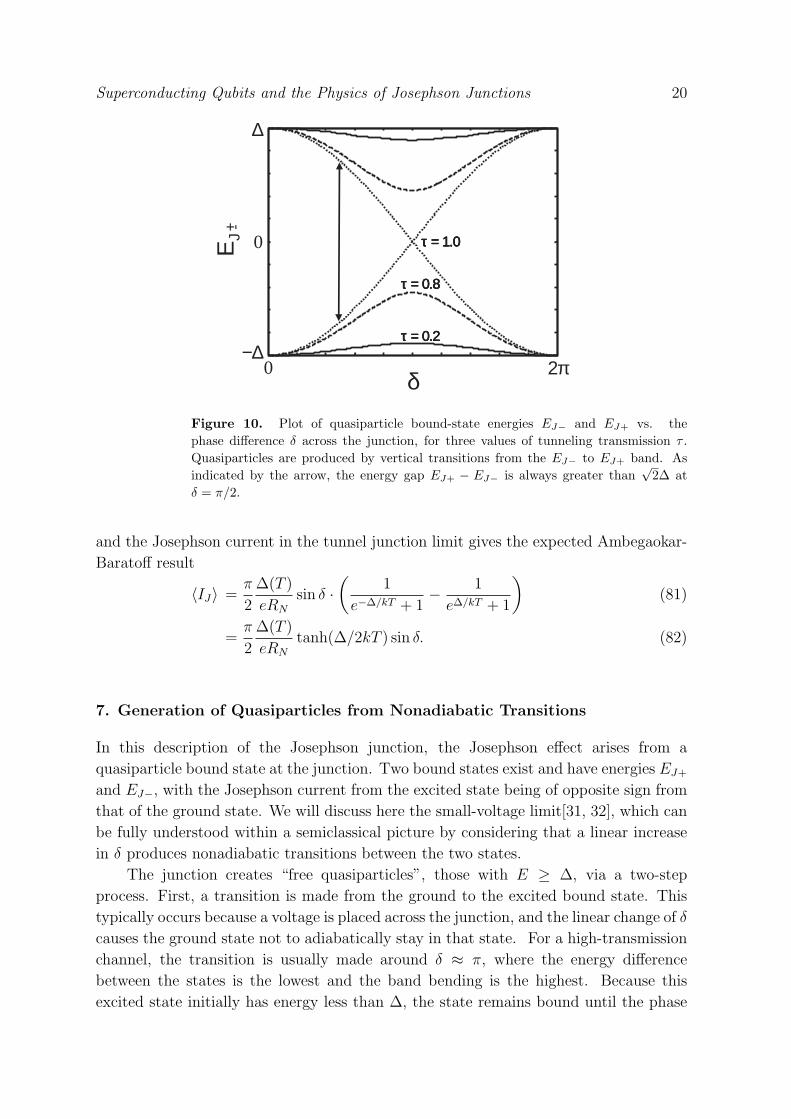
Superconducting Qubits and the Physics of Josephson Junctions 20
0 2π −∆
∆
0
δ
E J+
E J-
τ = 1.0 τ = 1.0 τ = 1.0 τ = 1.0
τ = 0.2 τ = 0.2 τ = 0.2 τ = 0.2
τ = 0.8 τ = 0.8 τ = 0.8 τ = 0.8
E J +
-
Figure 10. Plot of quasiparticle bound-state energies EJ− and EJ+ vs. thephase difference δ across the junction, for three values of tunneling transmission τ .Quasiparticles are produced by vertical transitions from the EJ− to EJ+ band. Asindicated by the arrow, the energy gap EJ+ − EJ− is always greater than
√2∆ at
δ = π/2.
and the Josephson current in the tunnel junction limit gives the expected Ambegaokar-
Baratoff result
〈IJ〉 =π
2
∆(T )
eRN
sin δ ·(
1
e−∆/kT + 1− 1
e∆/kT + 1
)(81)
=π
2
∆(T )
eRN
tanh(∆/2kT ) sin δ. (82)
7. Generation of Quasiparticles from Nonadiabatic Transitions
In this description of the Josephson junction, the Josephson effect arises from a
quasiparticle bound state at the junction. Two bound states exist and have energies EJ+
and EJ−, with the Josephson current from the excited state being of opposite sign from
that of the ground state. We will discuss here the small-voltage limit[31, 32], which can
be fully understood within a semiclassical picture by considering that a linear increase
in δ produces nonadiabatic transitions between the two states.
The junction creates “free quasiparticles”, those with E ≥ ∆, via a two-step
process. First, a transition is made from the ground to the excited bound state. This
typically occurs because a voltage is placed across the junction, and the linear change of δ
causes the ground state not to adiabatically stay in that state. For a high-transmission
channel, the transition is usually made around δ ≈ π, where the energy difference
between the states is the lowest and the band bending is the highest. Because this
excited state initially has energy less than ∆, the state remains bound until the phase
Superconducting Qubits and the Physics of Josephson Junctions 21
x V ( x )
R e { k } Im
{k }
E / ∆ R e { δ }
Im { δ
}
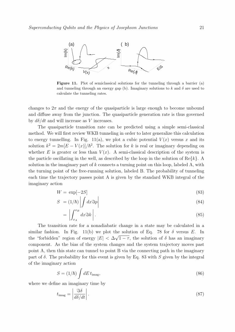
(a ) ( b)
Figure 11. Plot of semiclassical solutions for the tunneling through a barrier (a)and tunneling through an energy gap (b). Imaginary solutions to k and δ are used tocalculate the tunneling rates.
changes to 2π and the energy of the quasiparticle is large enough to become unbound
and diffuse away from the junction. The quasiparticle generation rate is thus governed
by dδ/dt and will increase as V increases.
The quasiparticle transition rate can be predicted using a simple semi-classical
method. We will first review WKB tunneling in order to later generalize this calculation
to energy tunnelling. In Fig. 11(a), we plot a cubic potential V (x) versus x and its
solution k2 = 2m[E − V (x)]/~2. The solution for k is real or imaginary depending on
whether E is greater or less than V (x). A semi-classical description of the system is
the particle oscillating in the well, as described by the loop in the solution of Re{k}. A
solution in the imaginary part of k connects a turning point on this loop, labeled A, with
the turning point of the free-running solution, labeled B. The probability of tunneling
each time the trajectory passes point A is given by the standard WKB integral of the
imaginary action
W = exp[−2S] (83)
S = (1/~)∣∣∣∣∫
dx=p
∣∣∣∣ (84)
=
∣∣∣∣∫ xB
xA
dx=k
∣∣∣∣ . (85)
The transition rate for a nonadiabatic change in a state may be calculated in a
similar fashion. In Fig. 11(b) we plot the solution of Eq. 78 for δ versus E. In
the “forbidden” region of energy |E| < ∆√
1− τ , the solution of δ has an imaginary
component. As the bias of the system changes and the system trajectory moves past
point A, then this state can tunnel to point B via the connecting path in the imaginary
part of δ. The probability for this event is given by Eq. 83 with S given by the integral
of the imaginary action
S = (1/~)∫
dE timag, (86)
where we define an imaginary time by
timag =
∣∣∣∣=δ
dδ/dt
∣∣∣∣ . (87)
Superconducting Qubits and the Physics of Josephson Junctions 22
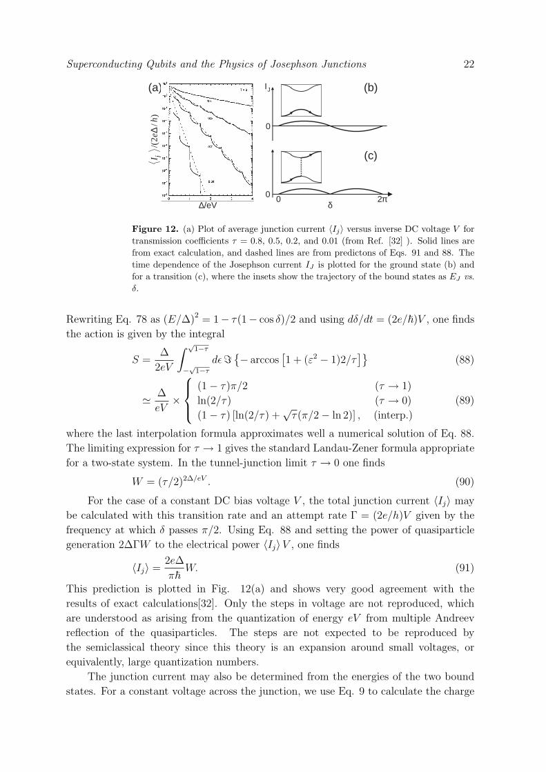
(a )
∆ /e V δ 2π 0
Ι J
0
0
(b )
(c ) )
/ 2
/(
h e
I ∆
j
Figure 12. (a) Plot of average junction current 〈Ij〉 versus inverse DC voltage V fortransmission coefficients τ = 0.8, 0.5, 0.2, and 0.01 (from Ref. [32] ). Solid lines arefrom exact calculation, and dashed lines are from predictons of Eqs. 91 and 88. Thetime dependence of the Josephson current IJ is plotted for the ground state (b) andfor a transition (c), where the insets show the trajectory of the bound states as EJ vs.δ.
Rewriting Eq. 78 as (E/∆)2 = 1− τ(1− cos δ)/2 and using dδ/dt = (2e/~)V , one finds
the action is given by the integral
S =∆
2eV
∫ √1−τ
−√1−τ
dε={− arccos[1 + (ε2 − 1)2/τ
]}(88)
' ∆
eV×
(1− τ)π/2
ln(2/τ)
(1− τ) [ln(2/τ) +√
τ(π/2− ln 2)] ,
(τ → 1)
(τ → 0)
(interp.)
(89)
where the last interpolation formula approximates well a numerical solution of Eq. 88.
The limiting expression for τ → 1 gives the standard Landau-Zener formula appropriate
for a two-state system. In the tunnel-junction limit τ → 0 one finds
W = (τ/2)2∆/eV . (90)
For the case of a constant DC bias voltage V , the total junction current 〈Ij〉 may
be calculated with this transition rate and an attempt rate Γ = (2e/h)V given by the
frequency at which δ passes π/2. Using Eq. 88 and setting the power of quasiparticle
generation 2∆ΓW to the electrical power 〈Ij〉V , one finds
〈Ij〉 =2e∆
π~W. (91)
This prediction is plotted in Fig. 12(a) and shows very good agreement with the
results of exact calculations[32]. Only the steps in voltage are not reproduced, which
are understood as arising from the quantization of energy eV from multiple Andreev
reflection of the quasiparticles. The steps are not expected to be reproduced by
the semiclassical theory since this theory is an expansion around small voltages, or
equivalently, large quantization numbers.
The junction current may also be determined from the energies of the two bound
states. For a constant voltage across the junction, we use Eq. 9 to calculate the charge
Superconducting Qubits and the Physics of Josephson Junctions 23
transferred across the junction after a phase change of 2π
Qj =
∫ 2π/(dδ/dt)
0
Ij dt (92)
=2π
Φ0
∫ 2π/(dδ/dt)
0
dUJ
dδdt (93)
=[UJ(2π)− UJ(0)]
V, (94)
which gives the expected result that the change of energy equals QjV . When the
junction remains in the ground state, the energy is constant UJ(2π) − UJ(0) = 0 and
no net charge flows through the junction. Net charge is transferred, however, after a
transition. The charge transfer 2∆/V multiplied by the transition rate gives an average
current QjΓW that is equivalent to Eq. 91.
Equation 80 may be used to calculate the time dependence of the Josephson current,
as illustrated in Fig. 12(b) and (c). When the system remains in the ground state (b),
the junction current is sinusoidal and averages to zero. For the case of a transition (c),
the current before the transition is the same, but the Josephson current remains positive
after the transition (see Eq. 5.4 of Ref. [32]). The transition itself also produces charge
transfer from multiple-Andreev reflections(MAR) [31, 33]
QMAR = 2∆(1− τ)1/2/V. (95)
This result is perhaps surprising - the junction current at finite voltage arises from
transfer of charge QMAR and a change in the Josephson current. The relative
contribution of these two currents is determined by the relative size of the gap in the
bound states. For τ → 1, all of the junction current is produced by Josephson current,
whereas for τ → 0 (tunnel junctions) the current comes from QMAR.
For small voltages, the transition event must transfer a large amount of charge
QMAR in order to overcome the energy gap. In comparing this semi-classical theory
with the exact MAR theory, QMAR/e has an integer value and represents the order of
the MAR process and the number of electrons that are transferred in the transition.
This description is consistent with Eq. 90 describing the transition probability for an
n-th order MAR process, where n = 2∆/eV , and τ/2 represents the matrix element for
each order.
From this example it is clearly incorrect to picture the quasiparticle and Josephson
current as separate entities, as suggested by the calculations of perturbation theory. To
do so ignores the fact that quasiparticle tunneling, arising from a transition between the
bound states, also changes the Josephson contribution to the current from δ = π to 2π.
8. Quasiparticle Bound States and Qubit Coherence
The quasiparticle bound-state theory can be used to predict both the Josephson and
quasiparticle current in the zero-voltage state, as appropriate for qubits. In this theory
an excitation from the EJ− bound state to the EJ+ state is clearly deleterious as
Superconducting Qubits and the Physics of Josephson Junctions 24
it will change the Josephson current, fluctuating the qubit frequency and producing
decoherence in the phase of the qubit state. For an excitation in one channel, the
fractional change in the Josephson current is ∼ 1/Nch, where Nch is the number of
conduction channels. The subgap current-voltage characteristics can be used to estimate
Nch, which gives an areal density of ∼ 104/µm2 [10, 34]. For a charge qubit with junction
area 10−2µm2, the qubit frequency changes fractionally by ∼ 1/Nch ∼ 10−2 for a single
excitation, and gives strong decoherence. Although the phase qubit has a smaller change
(1/Nch)I0/4(I0 − I) ∼ 2 × 10⁻⁵, the excitation of even a single bound state is clearly
unwanted.
Fortunately, these quasiparticle bound states should not be excited in tunnel
junctions by the dynamical behavior of the qubit. The EJ− to EJ+ transition is
energetically forbidden because the energy of the qubit states are typically choosen
to be much less than 2∆. Thus, the energy gap of the superconductor protects the
qubit from quasiparticle decoherence.
If a junction has “pinhole” defects, where a few channels have τ → 1, then the
energy gap will shrink to zero at δ = π. However, only the flux qubit will be sensitive
to quasiparticles produced at these defects since it operates near δ = π. In contrast, the
phase qubit always retains an energy gap of at least√
2∆ around its operating point
δ = π/2 (see arrow in Fig. 10). We note this idea implies that a phase qubit can even
be constructed from a microbridge junction, which has some channels[26] with τ = 1.
Although the phase qubit is completely insensitive to pinhole defects, this advantage
is probably unimportant because Al-based tunnel junctions have oxide barriers of good
quality.
Pinhole defects also change the Josephson potential away from the -cos δ form.
This modification is typically unimportant because the deviation is smooth and can be
accounted for by a small effective change in the critical current.
The concept that the energy gap ∆ protects the junction from quasiparticle
transitions suggests that superconductors with nonuniform gaps may not be suitable
for qubits. Besides the obvious problem of conduction channels with zero gap, channels
with a reduced gap may cause stray quasiparticles to be trapped at the junction. The
high-Tc superconductors, with the gap suppressed to zero at certain crystal angles, are
an obvious undesirable candidate. However, even Nb could be problematic since it has
several oxides that have reduced or even zero gap. Nb based tri-layers may also be
undesirable since the thin Al layer near the junction slightly reduces the gap around
the junction. In contrast, Al may not have this difficulty since its gap increases with
the incorporation of oxygen or other scattering defects. It is possible that these ideas
explain why Nb-based qubits do not have coherence times as long as Al qubits[6, 10].
9. Summary
In summary, Josephson qubits are nonlinear resonators whose critical element is the
nonlinear inductance of the Josephson junction. The three types of superconducting
Superconducting Qubits and the Physics of Josephson Junctions 25
qubits, phase, flux, and charge, use this nonlinearity differently and produce qubit
states from a cubic, quartic, and cosine potential, respectively.
To understand the origin and properties of the Josephson effect, we have first
reviewed the BCS theory of superconductivity. The superconducting phase was
explicitly shown to be a macroscopic property of the superconductor, whose classical
and quantum behavior is determined by the external electrical circuit. After a
review of quasiparticle and Josephson tunneling, we argued that a proper microscopic
understanding of the junction could arise only from an exact solution of the Josephson
effect.
This exact solution was derived by use of mesoscopic theory and quasiparticle
bound states, where we showed that Josephson and quasiparticle tunneling can be
understood from the energy of the bound states and their transitions, respectively.
A semiclassical theory was used to calculate the transition rate for a finite DC voltage,
with the predictions matching well that obtained from exact methods.
This picture of the Josephson junction allows a proper understanding of the
Josephson qubit state. We argue that the gap of the superconductor strongly protects
the junction from quasiparticle tunneling and its decoherence. We caution that an
improper choice of materials might give decoherence from quasiparticles that are trapped
at sites near the junction.
We believe a key to future success is understanding and improving this remarkable
nonlinearity of the Josephson inductance. We hope that the picture given here of the
Josephson effect will help researchers in their quest to make better superconducting
qubits.
10. Acknowledgements
We thank C. Urbina, D. Esteve, M. Devoret, and V. Shumeiko for helpful discussions.
This work is supported in part by the NSA under contract MOD709001.[1] M. A. Nielsen and I. L. Chuang, Quantum Computation and Quantum Information (Cambridge
University Press, Cambridge, 2000).[2] Y. Nakamura, C. D. Chen, and J. S. Tsai, Phys. Rev. Lett. 79, 2328 (1997).[3] Y. Nakamura, Y. A. Pashkin, T. Yamamoto, and J. S. Tsai, Phys. Rev. Lett. 88, 047901 (2002).[4] D. Vion, A. Aassime, A. Cottet, P. Joyez, H. Pothier, C. Urbina, D. Esteve, and M. H. Devoret,
Science 296, 886 (2002).[5] S. Han, Y. Yu, Xi Chu, S. Chu, and Z. Wang, Science 293, 1457 (2001); Y. Yu, S. Han, X. Chu,
S. Chu, and Z. Wang, Science 296, 889 (2002).[6] J. M. Martinis, S. Nam, J. Aumentado, and C. Urbina, Phys. Rev. Lett. 89, 117901 (2002).[7] I. Chiorescu, Y. Nakamura, C. J. P. M. Harmans, and J. E. Mooij, Science 299, 1869 (2003).[8] A.J. Berkley, H. Xu, R.C. Ramos, M.A. Gubrud, F.W. Strauch, P.R. Johnson, J.R. Anderson,
A.J. Dragt, C.J. Lobb, and F.C.Wellstood, Science 300, 1548 (2003).[9] Yu. A. Pashkin, T. Yamamoto, O. Astafiev, Y. Nakamura, D. V. Averin, and J. S. Tsai, Nature
421, 823 (2003).[10] R. W. Simmonds, K. M. Lang, D. A. Hite, D. P. Pappas, and J. M. Martinis, submitted to Phys.
Rev. Lett.
Superconducting Qubits and the Physics of Josephson Junctions 26
[11] M.H. Devoret, Quantum Fluctuations in Electrical Circuits, in “Fluctuations Quantiques”, ElsevierScience (1997).
[12] M. Steffen, J. M. Martinis, and I. L. Chuang, Phys. Rev. B 68, 2245xx (2003).[13] Audrey Cottet, Ph.D. thesis (2002).[14] R. Rouse, S. Han, J. Lukens, Phys. Rev. Lett. 75, 1614 (1995).[15] R. Koch, private communication.[16] J. E. Mooij, T. P. Orlando, L. Levitov, L. Tian, C. H. van der Wal, S. Lloyd, Science 285, 1036
(1999)[17] D. J. VanHarlingen, B. L. T. Plourde, T. L. Robertson, P. A Reichardt, and J. Clarke, Proceedings
of the 3rd International Workshop on Quantum Computing, to be published.[18] J. Bardeen, L. N. Cooper, and J. R. Schrieffer, Phys. Rev. 108, 1175 (1957).[19] P. W. Anderson, Phys. Rev. 112, 1900 (1958).[20] C. Kittel, Quantum Theory of Solids, John Wiley (1987).[21] U. Eckern, G. Schon, V. Ambegaokar, Phys. Rev. B 30, 6419 (1984).[22] V. Ambegaokar and A. Baratoff, Phys. Rev. Lett. 11, 104 (1963).[23] C. W. J. Beenakker, Phys. Rev. Lett. 67,3836 (1991).[24] C. W. J. Beenakker, Rev. Mod. Phys. 69, 731 (1997)[25] Y. Naveh, Vijay Patel, D. V. Averin, K. K. Likharev, and J. E. Lukens, Phys. Rev. Lett. 85, 5404
(2000).[26] O. N. Dorokhov, JETP Lett. 36, 318 (1982).[27] K. M. Schep and G. E. W. Bauer, Phys. Rev. Lett. 78, 3015 (1997).[28] A. Furusaki and M. Tsukada, Physica B 165-166, 967 (1990).[29] S. V. Kuplevakhaskii and I. I. Fal’ko, Sov. J. Low Temp. Phys. 17, 501 (1991).[30] Our notation for incoming and outgoing states is choosen to correspond to the boundry conditions
for scatttering in Ref. [32].[31] D. Averin and A. Bardas, Phys. Rev. Lett. 75, 1831 (1995).[32] E. N. Bratus’, V. S. Shumeiko, E. V. Bezuglyi, and G. Wendin, Phys. Rev. B 55, 12666 (1997).[33] E. N. Bratus, V. S. Shumeiko, and G. A. B. Wendin, Phys. Rev. Lett. 74, 2110 (1995).[34] K.M. Lang, S. Nam, J. Aumentado, C. Urbina, J. M. Martinis, IEEE Trans. on Appl. Supercon.
13, 989 (2003).


![Quantum Bits with Josephson Junctions · etc. [2]. This great reliance on Josephson junctions sets constraints on the operating temperature and frequency of the superconducting circuits](https://img.pdfslide.net/doc/110x75/5ec5592a13b08355f20aa431/quantum-bits-with-josephson-junctions-etc-2-this-great-reliance-on-josephson.jpg)