Embed Size (px)
Citation preview
1
Supercontinuum generation in media with sign-alternated dispersion
HAIDER ZIA1*, NIKLAS M. LÜPKEN2, TIM HELLWIG 2, CARSTEN FALLNICH2,1, KLAUS-J. BOLLER1,2 1 University of Twente, Department Science & Technology, Laser Physics and Nonlinear Optics Group,
MESA+ Research Institute for Nanotechnology, Enschede 7500 AE, The Netherlands 2 University of Münster, Institute of Applied Physics, Corrensstraße 2, 48149 Münster, Germany
Abstract:
When an ultrafast optical pulse with high intensity is propagating through transparent material
a supercontinuum can be coherently generated by self-phase modulation, which is essential to
many photonic applications in fibers and integrated waveguides. However, the presence of
dispersion causes stagnation of spectral broadening past a certain propagation length, requiring
an increased input peak power for further broadening. We present a concept to drive
supercontinuum generation with significantly lower input power by counteracting spectral
stagnation via alternating the sign of group velocity dispersion along the propagation. We
demonstrate the effect experimentally in dispersion alternating fiber in excellent agreement
with modeling, revealing almost an order of magnitude reduced peak power compared to
uniform dispersion. Calculations reveal a similar power reduction also with integrated optical
waveguides, simultaneously with a significant increase of flat bandwidth, which is important
for on-chip broadband photonics.
Introduction
Supercontinuum generation (SCG) is a nonlinear optical process where injecting intense,
ultrashort pulses in transparent optical materials generates light with ultra-wide spectral
bandwidth1–3. Maximum coherence is achieved when spectral broadening is dominated by self-
phase modulation based on the intensity dependent Kerr index4. The achieved bandwidths,
often spanning more than two octaves5–11 have become instrumental in a plethora of fields12.
Examples are metrology based on optical frequency combs13–17, optical coherence
tomography18–21, ranging22, or sub-cycle pulse compression23–25.
The widest spectral bandwidths at lowest input power are typically achieved in waveguiding
geometries, such as in fibers26–28 and integrated optical waveguides on a chip10,11,29,30 because
transverse confinement of light enhances the intensity, which promotes the nonlinear
generation of additional frequency components. However, although significant spectral
broadening can be achieved with low input power using highly nonlinear materials31,
generating bandwidth beyond one or two octaves still requires significant input peak powers in
the order of several kilowatt11,32,33, hundreds of kilowatt 34, or close to megawatt levels3,35. The
reason is that dispersion terminates spectral broadening beyond a certain propagation length,
which means that the peak power required for a desired bandwidth cannot be reduced by
extending the propagation length.
Such lack of scalability towards lower input power constitutes a critical limitation for
implementations of supercontinuum generation, specifically, in all-integrated optical systems.
In case of normal dispersion (positive group velocity dispersion) the reason for termination of
broadening is that initial pulse duration gets stretched and the waveguide-internal peak power
2
is lowered vs propagation. This brings self-phase modulation, the main mechanism of coherent
spectral broadening36, to stagnation past a certain propagation length4,36,37.
Lower input peak powers are sufficient with anomalous dispersion because negative group
velocity dispersion leads to pulse compression by making use of the additionally generated
bandwidth. However, spectral stagnation occurs again, here due to soliton formation, because
self-phase modulation comes into balance with anomalous dispersion1,38. At that point,
typically also soliton fission and Raman red-shifting occurs, and dispersive waves are
generated. However, fission does not increase the bandwidth1,36, dispersive waves generate only
disconnected components of narrowband radiation, and Raman conversion red-shifts the
frequency bandwidth, without increasing it.
For avoiding both pulse stretching and soliton formation, it seems desirable to provide zero
group velocity dispersion (GVD), to keep self-phase modulation ongoing and to increase the
bandwidth proportional to the interaction length. However, this would not yield the maximum
possible broadening with length, because newly generated spectral bandwidth is not used for
pulse compression during propagation.
We present a novel concept (see Fig.1) based on alternating the sign of group velocity
dispersion along propagation in a segmented medium. The alternation overcomes spectral
stagnation and thereby lowers the input peak power and pulse energy required for
supercontinuum generation. In its simplest setting, self-phase modulation in normal dispersive
segments generates spectral broadening and subsequent segments with anomalous dispersion
make use of the newly generated bandwidth for pulse re-compression and peak power increase,
which lets spectral broadening continue. An approximate analysis reveals close-to-exponential
growth of bandwidth vs propagation at weak dispersion and linear growth at strong dispersion.
This scaling with interaction length enables to generate a given spectral bandwidth with
substantially reduced pulse energy and peak power as compared to conventional
supercontinuum generation based on uniform dispersion.
Results
Basic dynamics with alternating dispersion
Figure 1 shows calculated developments of the optical spectrum and pulse along propagation
for a dispersion alternated waveguide (Fig. 1A) made of normal dispersive (ND) segments
(positive group velocity dispersion) and anomalous dispersive (AD) segments (negative group
velocity dispersion). For unveiling the novel spectral dynamics caused by alternating
dispersion, the calculations retain only the two main physical processes, which are self-phase
modulation (SPM) causing coherent spectral broadening and second-order dispersion
responsible for temporal stretching or compressing the pulse. For convenience, we take
transform limited Gaussian pulses as input and consider spectral broadening only in the ND
segments. Other situations, e.g., non-Gaussian input pulses, spectral broadening in both types
of segments, higher-order dispersion, or propagation loss are taken into account as well, when
comparing with experimental data as in Figs. 2 and 3.
Figure 1 B shows the increase in spectral bandwidth vs propagation coordinate as obtained
by numerical integration of the nonlinear Schrödinger equation (NLSE) using parameters as in
telecom ND and AD fiber (Supplementary Section 1). It can be seen that there is an initial
spectral broadening through SPM in the first ND segment, but broadening stagnates beyond
approximately 𝑧1=15 cm. The reason for stagnation in this ND segment is loss of peak intensity
and increased duration by normal dispersive temporal broadening of the pulse (Fig. 1C).
To re-initiate spectral broadening by re-establishing high peak intensity, the pulse is
temporally re-compressed in an AD segment back to its transform limit (between 𝑧1 and 𝑧2=30
cm).

3
A
B C
D E
Figure 1: Supercontinuum generation (SCG) using alternating dispersion A: Waveguide with segments of
normal dispersion (ND, red) and anomalous dispersion (AD, yellow). The basic pulse and spectral propagation
dynamics is modelled with Gaussian input pulses using parameters as in telecom fiber (Supplementary Section
1), accounting for second-order dispersion in ND and AD segments, and self-phase modulation in the ND
segments. B: Normalized energy density spectrum vs. propagation with alternating dispersion. C: Intensity and
shape of the pulse vs propagation. Undesired pulse stretching in the bandwidth generating (ND) segments is
repeatedly compensated by anomalous dispersive (AD) segments. D: Spectral bandwidth of supercontinuum
generation in alternating dispersion (ND-AD) compared to zero uniform dispersion (zero GVD), and to uniform
normal and anomalous dispersion (uniform AD, uniform ND). For direct comparison with the uniform
waveguides the graph omits non-generating AD segments. With the chosen fiber parameters and input pulse,
alternating dispersion yields close-to-exponential growth (blue-shaded exponential fit curve under blue trace).
Supercontinuum generation in uniform ND and AD exhibits spectral stagnation. E: Calculated spectral
bandwidth increasement factor, 𝐹, in single ND segments vs the relative strength of dispersion and self-phase
modulation, 𝑅, in terms of the ratio of nonlinear length to dispersive length (𝑅 = 𝐿𝑛𝑙/𝐿𝑑).
4
The pulse at 𝑧2 is shorter and has a higher intensity than the incident pulse (𝑧0= 0 cm) because
SPM in the first ND segment has increased the bandwidth above that of the input pulse. The
consequence of higher intensity and shorter pulse duration is that SPM in the second ND
segment yields more additional bandwidth (between 𝑧2 and 𝑧3) than what was gained in the
first ND segment (between 𝑧0 and 𝑧1). Also, the rate of bandwidth growth and dispersion are
higher, so that spectral stagnation is reached after a shorter propagation distance than in the first
ND segment. Following this concept, further dispersion alternating segments keep the
bandwidth growing and let the pulse become shorter as shown.
Fig. 1 D provides a bandwidth comparison with conventional supercontinuum generation
(uniform AD, uniform ND) where the growth of bandwidth stagnates. In alternating dispersion
(ND-AD), bandwidth generation remains ongoing with each next ND segment (AD segments
omitted in for direct comparison with generation in uniform AD and ND media). With the
chosen fiber and pulse parameters, the spectral bandwidth grows close-to-exponential (see
blue-shaded exponential fit curve) and reaches about 200 THz via SPM in 50 cm of bandwidth
generating ND segments. In uniformly dispersive fiber (ND or AD) there is spectral stagnation,
limiting the bandwidth to 15 THz (after 20 cm) and 20 THz (after 10 cm), respectively.
The bandwidth at stagnation in uniform dispersion may be increased as well, however, this
requires significantly increased power, because the bandwidth grows approximately only with
the square-root of the input power1,4,36. For instance, generating 200 THz in uniform dispersion
with the fiber parameters used in Fig.1, would require about 180-times higher power (with ND),
and 100-times higher power with uniform AD. The bandwidth comparison in Fig. 1 D is thus
indicating that alternating dispersion allows to significantly reduce the power required for
generating a given bandwidth.
Scaling of bandwidth with segment number and input power Many applications benefit from a broad spectral bandwidth particularly if there is significant
power also at the edges of the specified bandwidth, i.e., if spectra are approximately flat in the
range of interest36,37. The standard definition of bandwidth for supercontinuum generation leads
to wider bandwidth values as it accepts low power at the edges, typically at the -30-dB level.
To follow a conservative definition of bandwidth addressing approximately flat spectra, we
chose as bandwidth, Δ𝜈, the full width frequency bandwidth at the 1/e-level of the energy
spectral density.
To provide spectra with minimum interference structure4,36,37, we continue considering that
spectral broadening is generated in the ND segments with Gaussian pulses, and that the AD
segments just re-compress the pulse to the transform limited duration, Δ𝑡 ∙ Δ𝜈 = 2 𝜋⁄ , where
Δ𝑡 is the 1/e half-width duration.
For calculating the bandwidth increase in a particular ND segment when a transform limited
pulse enters the segment, it is important to realize that the achievable broadening is ruled by
only two parameters. The first is the nonlinear length, 𝐿𝑛𝑙 = 1/(𝛾𝑃), depending reciprocally
on the peak power 𝑃, where 𝛾 is the nonlinear coefficient of the ND segment. 𝐿𝑛𝑙 denotes the
propagation length where the bandwidth increases by a factor √5 if dispersion were absent39.
The second parameter is the dispersion length, 𝐿𝑑 = Δ𝑡2/|𝛽2| depending quadratically on the
pulse duration, where 𝛽2 is the coefficient for second-order (group velocity) dispersion39. 𝐿𝑑
denotes the propagation length after which the pulse duration increases by a factor of √2 if
SPM were absent.
Given a certain length of the ND segment, it is the ratio of 𝐿𝑛𝑙 and 𝐿𝑑 which determines the
bandwidth gained in that segment. For instance, if dispersion is weak compared to spectral
broadening, i.e., if the ratio 𝑅 = 𝐿𝑑 𝐿𝑛𝑙⁄ is small (𝑅 ≪ 1), one expects the bandwidth to increase
5
by a factor of 𝐹 = √5 if the segment length is chosen equal to the nonlinear length. If dispersion
is strong vs SPM, due to a short pulse duration and thus a wide spectrum (𝑅 ≫ 1), there will
still be broadening in the beginning of the segment, but the bandwidth increasement factor will
only be slightly above unity, 𝐹 ≳ 1.
To quantify the relation between the ratio 𝑅 and spectral broadening in an ND segment, we
devise a lower-bound calculation of the bandwidth increasement factor, 𝐹(𝑅), and display the
result in Fig.1E (see derivation of 𝐹( 𝑅) in Supplementary Section 2). For the calculation, we
chose the length of the ND segment to be its nonlinear length, to encompass all nonlinear
generation up to the point where the bandwidth stops increasing. It can be seen that 𝐹 varies
with 𝑅 as expected, i.e., having its values close to √5 at small 𝑅 and reducing asymptotically
to unity towards increasing 𝑅.
We note that 𝐹(𝑅) does not only determine the broadening in a single ND segment, but it
determines also the broadening in all following ND segments. To illustrate this, we recall Fig.1
where, due to recompression in AD segments, the peak power increases and pulse duration
shortens before entering a next ND segment. This causes 𝑅 to increase with each ND segment
since 𝑅 ∝ 1 Δ𝑡⁄ . More specifically, because the 𝑅-value of a previous ND segment determines
the bandwidth increasement factor 𝐹 in the according segment (see Fig. 1 E), it also determines
the bandwidth, transform limited pulse duration and peak power in front of the next ND
segment. The peak power and pulse duration then set the 𝑅-value of the next ND segment and,
via 𝐹(𝑅), the next bandwidth increase. Labelling the ND segment number with 𝑝, the recursive
dependence of 𝑅𝑝 on 𝑅𝑝−1 is why the first segment, 𝑅1, pre-determines the bandwidth growth
along the entire structure.
The bandwidth at the end of the structure with a number of 𝑛 ND segments, if Δ𝜈0 is the
frequency bandwidth of the incident pulse, can then be expressed as a product of broadening
factors,
∆𝜈𝑛 = ∆𝜈0 ∙ ∏ 𝐹𝑝𝑛𝑝=1 . Eq.1
Here 𝐹𝑝 ≡ Δ𝜈𝑝 Δ𝜈𝑝−1⁄ is the bandwidth increasement factor of the 𝑝𝑡ℎ ND segment, where
Δ𝜈𝑝−1 is the bandwidth in front of the segment and Δ𝜈𝑝 is the bandwidth behind the segment.
Particularly strong growth is obtained from Eq.1 if generation remains in the range of
relatively weak dispersion (𝑅 ≤ 1)). In this case 𝐹𝑃 remains close to its maximum value
(𝐹𝑃(0) = √5 ≈ 2.23) or decreases only slowly with segment number. The bandwidth growth
then remains approximately exponential with the number of ND segments, resulting in
∆𝜈𝑛 = ∆𝜈0 ∙ 𝐹𝑛 , Eq. 2
as is found also numerically for the example in Fig. 1D. In the other limit of strong
dispersion (𝑅 ≫ 1), we find (more details in Supplementary Section 3) that the decrease in 𝐹𝑃
with each additional ND segment reduces Eq.1 to a linear growth of bandwidth with the number
of ND segments,
Δ𝜈𝑛 ≈ 𝑛 [𝑔𝑜𝛾2𝐸
4|𝛽2|] + ∆𝜈0 , Eq. 3
with 𝑔𝑜 ≈ 0.81 being a constant related to the Gaussian pulse shape, and with
𝐸 = √𝜋 𝑃 ∙ Δt being the pulse energy.
Equations 2 and 3 display that the basic dynamics of supercontinuum generation in
alternating dispersion is a growth of spectral bandwidth vs propagation length, while with
uniform dispersion spectral stagnation occurs. The growth may remain close to exponential if
𝑅 remains small throughout all segments, show transition from exponential to linear growth at

6
around a certain segment number 𝑛𝑇 where 𝑅 ≈ 1, or is close to linear if dispersion is strong
in the first and thus also in all segments (𝑅1 ≫ 1).
Using these properties, we find approximate bandwidth-to-input peak power scaling laws
(more details in Supplementary Section 3) shown in Table 1. In uniform dispersion there is only
a square-root growth of bandwidth vs input peak power. With alternating dispersion, the
bandwidth increases in a mixture of exponential and linear growth vs input peak power, where
the slope and exponent can be increased monotonically with the total number of ND segments.
Correspondingly, the generated bandwidth changes much more strongly with input peak power
in the alternating dispersion structure. Therefore, the power required to achieve a given
bandwidth can be much reduced by increasing the number of ND segments.
Relative strength of
dispersion over self-phase
modulation
in first segment
Scaling of bandwidth with
input peak power using
alternating dispersion
Scaling of
bandwidth
with
uniform
dispersion
𝑅1 > 1 to 𝑅1 ≲ 1
Δ𝜈𝑛 ∝ (𝑐𝑇√𝑃𝑂)𝑛𝑡−1 + (𝑛 − 𝑛𝑡 + 1)𝑃𝑂 Δ𝜈𝑛 ∝ 𝑃𝑜
12
𝑅1 ≪ 1 Δ𝜈𝑛 ∝ [𝑐𝑇𝑛𝑡−1 + (𝑛 − 𝑛𝑡 + 1)]𝑃𝑂 Δ𝜈𝑛 ∝ 𝑃𝑜
12
Table 1: Scaling of bandwidth vs input peak power, 𝑷𝟎, and number of segments, 𝒏, compared to power scaling in
uniform dispersion. Alternating dispersion yields a mixture of linear and exponential growth vs the input peak power, depending on the relative strength of dispersion over self-phase modulation in the first ND section (expressed as the
ratio of nonlinear length to dispersive length, 𝑹(𝟏) = 𝑳𝒏𝒍(𝟏)
/𝑳𝒅(𝟏)
. 𝒏𝑻 is the segment number where exponential growth
transits into linear growth (where 𝑹 ≈ 𝟏), and 𝒄𝑻 is a constant (see Supplementary Section 3 regarding the definition
of 𝒏𝑻 and 𝒄𝑻)
Experimental results
For demonstrating increased spectral broadening with alternating dispersion, we use
supercontinuum generation with ultra-short optical pulses injected into a dispersion alternated
optical fiber structure shown in Fig. 2A. The incident pulses have 74 fs FWHM pulse duration
at 50 mW average power and 79.9 MHz repetition rate (central wavelength of 1560 nm). The
pulses are provided by a mode-locked Erbium doped fiber laser, amplifier and a temporal
compressor system. The power coupled into the fiber is 35.6 mW (446 pJ pulse energy) and
is held constant throughout the main experiments.
The dispersion alternated fiber structure is selected to comprise alternating segments of
standard single-mode ND and AD telecom fiber with well-characterized linear and nonlinear
properties (see Fig. 2B and parameters in Supplementary Section 4) because this enables
numerical modeling with high reliability. We note that the wavelength range across which the
sign of the dispersion can be alternated and the concept can be applied, is ultimately given by
the ND and AD zero-dispersion wavelengths indicated with dashed lines in Fig. 2B.
In the experiment, ND and AD segments are added sequentially, with the choice of segment
length guided by intermittent recordings of the energy spectrum and the pulse duration (see
Methods). Due to the almost five-times higher nonlinear coefficient in the ND fiber compared
to the AD fiber, spectral broadening comes almost entirely from the ND segments, similar to
the setting used for illustrating the basic dynamics in Fig.1.

7
Figure 2C shows supercontinuum spectra measured behind each added ND segment.
Starting with the injected light, the spectral bandwidth increases with each ND segment. For
better analysis, Fig. 2D displays the measured bandwidth growth vs segment number (red dots).
To identify the regime of growth, we determine the experimental ratio 𝑅 = 𝐿𝑛𝑙 𝐿𝑑⁄ using the
measured peak power and pulse duration. We find 𝑅 ≤ 1 for the first two segments, suggesting
that the initial growth would be closer to exponential growth, while the third and fourth
segments would introduce a transition towards linear growth. This is confirmed by finding a
slightly upwards curved growth along the first three data points, followed by a transit towards
more linear growth with the remaining segments.
The maximum number of ND segments before no further spectral broadening occurs is seen
to be four. This can be addressed to the finite width of the spectral interval across which
dispersion parameters show opposite signs (Fig. 2B), i.e., the range in which alternating
dispersion can be applied with the used fibers.
Figure 2E shows supercontinuum spectra generated with dispersion alternated fiber with
four ND segment (trace 1). For direct bandwidth comparison, we generate supercontinuum also
in uniform fiber (trace 2 and 3 for uniform ND and AD fiber, respectively), using the same
input pulse parameters and fiber length. The comparison shows that alternating dispersion
increases the full 1/e bandwidth by a factor of 1.4 and 2.5 with regard to uniform ND and AD
fiber, respectively. The full-width at -30 dB increases by a factor of 2.5 and 3.1, respectively.
The dashed traces are numerical solutions of the generalized nonlinear Schrödinger equation,
accounting for all orders of dispersion, the experimental pulse shape, loss between segments,
and also weak SPM in the AD segments (see parameters in Supplementary Section 4). It can
be seen that there is very good agreement with the experimental data in all cases, i.e., for
supercontinuum generation in uniform ND and AD fiber, and also for the dispersion alternated
fiber.
Figures 2F compares the development of the pulse duration with according measurements
of the intensity autocorrelation (Fig. 2G). We find good agreement between the modelled
oscillation of the pulse duration with that of the autocorrelation measurements.
Motivated by the agreement and given the spectral bandwidth generated with dispersion
alternated fiber, we use the model to extrapolate the pulse energy needed to generate the same
bandwidth with uniform ND fiber. The model predicts that approximately one order of
magnitude higher pulse energy is required with uniform dispersion. We note that this factor is
a conservative number due to splice loss between segments (about 8% per splice) which lowers
the intensity available for SPM towards the later segments. Lower required powers are expected
with post-processing the splices. The presence of non-compensated third and higher-order
dispersion (see Fig. 2B) is indicating a certain robustness of sign-alternating dispersion vs
higher-order dispersion.

8
A B C D E F G
Figure 2: A) Experimental setup for supercontinuum generation (SCG) in optical fiber with alternating normal
dispersion (ND) and anomalous dispersion (AD). HWP: half-wave plate. PBS: polarization beam splitter. L1, L2:
lenses. SM: switchable mirror. OSA: optical spectrum analyzer. AC: autocorrelator. B) Dispersion parameter, 𝐷 =𝛽2 ∙ (2𝜋𝑐 𝜆2⁄ ), vs wavelength of the AD and ND fiber segments. The wavelengths of zero second-order dispersion are
indicated with dotted vertical lines. C) Relative spectral energy density of supercontinuum generation measured behind each ND segment (NDS) in the alternating waveguide structure. The spectral bandwidth grows in steps with added
ND segments. D) Measured bandwidth vs ND segment number retrieved from the spectra in C. The measured pulse
duration and peak power entering the segments, used to determine the 𝑅-value for each segment (not separately
shown), suggest an approximately exponential growth via the first two segments (compare to exponential curve beginning at input bandwidth). Thereafter, weaker growth transiting to linear is expected. E) Measured normalized
spectral energy density at the end of the dispersion alternating fiber (violet trace). For direct bandwidth comparison,
measured supercontinuum spectra obtained with uniform ND fiber (yellow trace) and AD fiber (red) of the same length are shown, generated with the same input pulse parameters. The dotted traces show theoretical spectra obtained with
9
the generalized nonlinear Schrödinger equation, using the experimental input spectrum, containing the full fiber dispersion (B) and weak SPM also in the AD segments. F) Calculated normalized intensity (color coded) vs time
(horizontal axis) and vs the propagation coordinate (vertical axis). Dotted white lines indicate the transitions between
ND and AD segments. G) Measured width of auto-correlation trace (FWHM) versus propagation distance in the dispersion alternated fiber. The dotted trace connects experimental data. The re-compressed pulse is becoming shorter
after each further AD segment.
Integrated optical waveguides with alternating dispersion
Particularly promising is supercontinuum generation in integrated optical waveguides because
tight guiding reduces the required input power to provide high intensities. Further advantages
are that lithographic fabrication methods provide increased freedom and precision in dispersion
engineering40. For instance, different from fiber splicing, transitions between segments can be
shaped as desired, and also the spectral shape of ND and AD dispersion may be designed to
widen the wavelength range between ND and AD zero dispersion wavelengths.
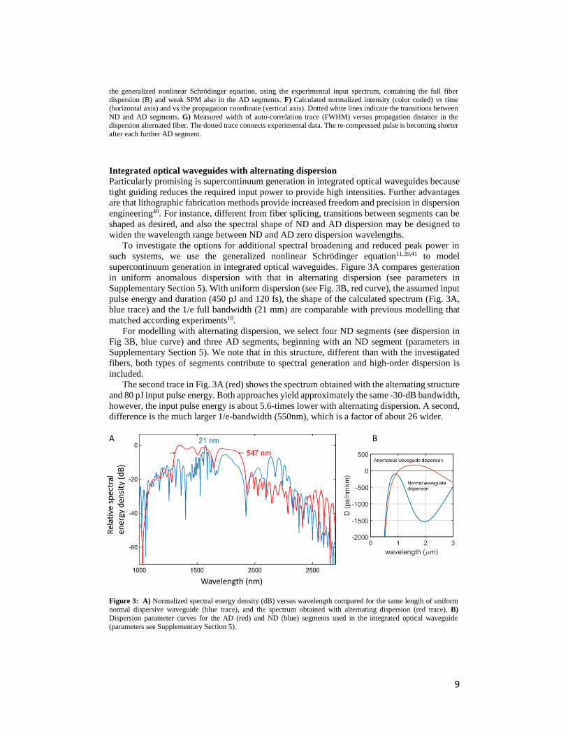
To investigate the options for additional spectral broadening and reduced peak power in
such systems, we use the generalized nonlinear Schrödinger equation11,39,41 to model
supercontinuum generation in integrated optical waveguides. Figure 3A compares generation
in uniform anomalous dispersion with that in alternating dispersion (see parameters in
Supplementary Section 5). With uniform dispersion (see Fig. 3B, red curve), the assumed input
pulse energy and duration (450 pJ and 120 fs), the shape of the calculated spectrum (Fig. 3A,
blue trace) and the 1/e full bandwidth (21 mm) are comparable with previous modelling that
matched according experiments10.
For modelling with alternating dispersion, we select four ND segments (see dispersion in
Fig 3B, blue curve) and three AD segments, beginning with an ND segment (parameters in
Supplementary Section 5). We note that in this structure, different than with the investigated
fibers, both types of segments contribute to spectral generation and high-order dispersion is
included.
The second trace in Fig. 3A (red) shows the spectrum obtained with the alternating structure
and 80 pJ input pulse energy. Both approaches yield approximately the same -30-dB bandwidth,
however, the input pulse energy is about 5.6-times lower with alternating dispersion. A second,
difference is the much larger 1/e-bandwidth (550nm), which is a factor of about 26 wider.
A B
Figure 3: A) Normalized spectral energy density (dB) versus wavelength compared for the same length of uniform normal dispersive waveguide (blue trace), and the spectrum obtained with alternating dispersion (red trace). B)
Dispersion parameter curves for the AD (red) and ND (blue) segments used in the integrated optical waveguide
(parameters see Supplementary Section 5).

10
Conclusions
Alternating the sign of dispersion in supercontinuum generation is a novel and highly
promising concept for increasing the generated spectral bandwidth and for reducing the
required input peak power or pulse energy. Even in a situation where the -30-dB bandwidth is
already extremely wide, the flat part of the spectrum specified via the 1/e bandwidth can be
much increased and, simultaneously, the required power can be much reduced.
We note that, in the limit of linear optics, dispersive sign alternation is well known in optical
fiber communications for preventing pulse stretching, and to ensure that the dynamics remains
in the linear regime, to avoid cross-talk of pulses42,43. Periodic dispersion oscillation is also
known for providing quasi-phase matching (QPM) of dispersive waves with solitons, for
enhancing spectrally narrowband modulation instability, or to generate soliton trains44,45.
The concept of alternating dispersion presented here goes far beyond, because it offers
wider bandwidth at reduced power. Due to its generality, we expect that the concept can have
important impact in a large variety of waveguiding systems that aim at coherent generation of
broadband optical light fields. Examples may include photonic crystal fibers46, low-power
broadband generation for dual-comb applications in the mid-infrared47, on-chip generation of
frequency combs48, and coherent spectral broadening in liquid49 and gaseous media50.
The basic concept as presented, encourages further investigations into various directions.
For instance, spectrally shaping normal and anomalous dispersion via dispersion engineering
in photonics waveguides can be explored to extend the range between zero-dispersion
wavelengths. Emphasizing self-phase modulation in normal dispersive segments, rather than in
anomalous dispersion, might be used to reduce undesired spectral structure, nonlinear phase
spectra, and noise from modulation instability, as is found in supercontinuum generation with
anomalous dispersion4,36,37.
For optimum results, i.e., maximally wide spectra at lowest possible power, alternating
dispersion requires an optimum choice of the segment lengths. Sets of adjacent waveguide
structures on chip may be used to cope with wider variations of the input power or pulse shape.
Nevertheless, because alternating dispersion always counteracts the detrimental effects of
uniform dispersion, we observe that noticeably increased bandwidth and lowered power
requirements can be obtained even with non-optimally matched segment lengths, for instance
with simple periodic sign-alternation.
References
1. Dudley, J. M., Genty, G. & Coen, S. Supercontinuum generation in photonic crystal
fiber. Rev. Mod. Phys. 78, 1135–1184 (2006).
2. Toulouse, J. Optical nonlinearities in fibers: Review, recent examples, and systems
applications. J. Light. Technol. 23, 3625–3641 (2005).
3. Schenkel, B., Paschotta, R. & Keller, U. Pulse compression with supercontinuum
generation in microstructure fibers. J. Opt. Soc. Am. B 22, 687 (2005).
4. Heidt, A. M., Feehan, J. S., Price, J. H. V. & Feurer, T. Limits of coherent
supercontinuum generation in normal dispersion fibers. J. Opt. Soc. Am. B 34, 764
(2017).
5. Silva, F. et al. Multi-octave supercontinuum generation from mid-infrared
filamentation in a bulk crystal. Nat. Commun. 3, 805–807 (2012).
6. Couny, F. et al. Generation and Photonic. Science (80-. ). 318, 1118–1121 (2007).

11
7. Seidel, M. et al. Multi-watt, multi-octave, mid-infrared femtosecond source. Sci. Adv.
4, eaaq1526 (2018).
8. Lemière, A. et al. Mid-infrared supercontinuum generation from 2 to 14 μm in
arsenic- and antimony-free chalcogenide glass fibers. J. Opt. Soc. Am. B 36, A183
(2019).
9. Granzow, N. et al. Supercontinuum generation in chalcogenide-silica step-index
fibers. Opt. Express 19, 21003 (2011).
10. Porcel, Marco A.G. et al. Two-octave spanning supercontinuum generation in
stoichiometric silicon nitride waveguides pumped at telecom wavelengths. Opt.
Express 25, 1542 (2017).
11. Epping, J. P. et al. On-chip visible-to-infrared supercontinuum generation with more
than 495 THz spectral bandwidth. Opt. Express 23, 19596 (2015).
12. Dudley, J. M. & Taylor, J. R. Ten years of nonlinear optics in photonic crystal fibre.
Nat. Photonics 3, 85–90 (2009).
13. Yu, M. et al. Silicon-chip-based mid-infrared dual-comb spectroscopy. Nat. Commun.
9, 6–11 (2018).
14. Luke, K., Okawachi, Y., Lamont, M. R. E., Gaeta, A. L. & Lipson, M. Broadband
mid-infrared frequency comb generation in a Si3N4 microresonator. Opt. Lett. 40,
4823 (2015).
15. Schliesser, A., Picqué, N. & Hänsch, T. W. Mid-infrared frequency combs. Nat.
Photonics 6, 440–449 (2012).
16. Rieker, G. B. et al. Frequency-comb-based remote sensing of greenhouse gases over
kilometer air paths. Optica 1, 290 (2014).
17. Holzwarth, R. Optical frequency metrology. Nature 416, 1–5 (2002).
18. Humbert, G. et al. Supercontinuum generation system for optical coherence
tomography based on tapered photonic crystal fibre. Opt. Express 14, 1596 (2006).
19. Unterhuber, A. et al. Advances in broad bandwidth light sources for ultrahigh
resolution optical coherence tomography. Phys. Med. Biol. 49, 1235–1246 (2004).
20. Israelsen, N. M. et al. Real-time high-resolution mid-infrared optical coherence
tomography. Light Sci. Appl. 8, (2019).
21. Nishizawa, N., Chen, Y., Hsiung, P., Ippen, E. P. & Fujimoto, J. G. Real-time,
ultrahigh-resolution, optical coherence tomography with an all-fiber, femtosecond
fiber laser continuum at 15 µm. Opt. Lett. 29, 2846 (2004).
22. Chen, Y. et al. Two-channel hyperspectral LiDAR with a supercontinuum laser
source. Sensors 10, 7057–7066 (2010).
23. Manzoni, C. et al. Coherent pulse synthesis: Towards sub-cycle optical waveforms.
Laser Photonics Rev. 9, 129–171 (2015).
24. Hassan, M. T. et al. Optical attosecond pulses and tracking the nonlinear response of
bound electrons. Nature 530, 66–70 (2016).
25. Hemmer, M., Baudisch, M., Thai, A., Couairon, A. & Biegert, J. Self-compression to
sub-3-cycle duration of mid-infrared optical pulses in dielectrics. Opt. Express 21,
28095 (2013).
26. Omenetto, F. G. et al. Spectrally smooth supercontinuum from 350 nm to 3 μm in
sub-centimeter lengths of soft-glass photonic crystal fibers. Opt. Express 14, 4928
(2006).
27. Wadsworth, W. J. et al. Supercontinuum generation in photonic crystal fibers and
optical fiber tapers: a novel light source. J. Opt. Soc. Am. B 19, 2148 (2008).
28. Pricking, S. & Giessen, H. Tailoring the soliton and supercontinuum dynamics by
engineering the profile of tapered fibers. Opt. Express 18, 20151 (2010).
29. Moss, D. J., Morandotti, R., Gaeta, A. L. & Lipson, M. New CMOS-compatible
platforms based on silicon nitride and Hydex for nonlinear optics. Nat. Photonics 7,
597–607 (2013).
12
30. Lamont, M. R., Luther-Davies, B., Choi, D.-Y., Madden, S. & Eggleton, B. J.
Supercontinuum generation in dispersion engineered highly nonlinear (γ = 10 /W/m)
As2S3 chalcogenide planar waveguide. Opt. Express 16, 14938 (2008).
31. Yeom, D.-I. et al. Low-threshold supercontinuum generation in highly nonlinear
chalcogenide nanowires. Opt. Lett. 33, 660 (2008).
32. Zhang, R., Teipel, J. & Giessen, H. Theoretical design of a liquid-core photonic
crystal fiber for supercontinuum generation. Opt. Express 14, 6800 (2006).
33. Singh, N. et al. Midinfrared supercontinuum generation from 2 to 6 μm in a silicon
nanowire. Optica 2, 797 (2015).
34. Tauser, F., Leitenstorfer, A. & Zinth, W. Amplified femtosecond pulses from an
Er:fiber system: Nonlinear pulse shortening and selfreferencing detection of the
carrier-envelope phase evolution. Opt. Express 11, 594 (2010).
35. Petersen, C. R. et al. Mid-infrared supercontinuum covering the 1.4-13.3 μm
molecular fingerprint region using ultra-high NA chalcogenide step-index fibre. Nat.
Photonics 8, 830–834 (2014).
36. Alfano, R. R. The supercontinuum laser source: the ultimate white light. (Springer
US, 2016).
37. Heidt, A. M. Pulse preserving flat-top supercontinuum generation in all-normal
dispersion photonic crystal fibers. J. Opt. Soc. Am. B 27, 550–559 (2010).
38. Islam, M. N. et al. Femtosecond distributed soliton spectrum in fibers. J. Opt. Soc.
Am. B 6, 1149 (2008).
39. Lin, Q., Painter, O.J., Agrawal, G. P. et al. Nonlinear optical phenomena in silicon
waveguides. Opt. Express 15, 16604–16644 (2006).
40. Wörhoff, K., Heideman, R. G., Leinse, A. & Hoekman, M. TriPleX: a versatile
dielectric photonic platform. Adv. Opt. Technol. 4, 189–207 (2015).
41. Kues, M., Brauckmann, N., Walbaum, T., Groß, P. & Fallnich, C. Nonlinear
dynamics of femtosecond supercontinuum generation with feedback. Opt. Express 17,
15827 (2009).
42. Mollenauer, L. F., Mamyshev, P. V. & Neubelt, M. J. Method for facile and accurate
measurement of optical fiber dispersion maps. Opt. Lett. 21, 1724 (2008).
43. Richardson, L. J., Forysiak, W. & Doran, N. J. Dispersion-managed soliton
propagation in short-period dispersion maps. Opt. Lett. 25, 1010 (2007).
44. Hickstein, D. D. et al. Quasi-Phase-Matched Supercontinuum Generation in Photonic
Waveguides. Phys. Rev. Lett. 120, 53903 (2018).
45. Copie, F., Kudlinski, A., Conforti, M., Martinelli, G. & Mussot, A. Modulation
instability in amplitude modulated dispersion oscillating fibers. Opt. Express 23, 3869
(2015).
46. Paulsen, H. N., Hilligse, K. M., Thøgersen, J., Keiding, S. R. & Larsen, J. J. Coherent
anti-Stokes Raman scattering microscopy with a photonic crystal fiber based light
source. Opt. Lett. 28, 1123 (2007).
47. Millot, G. et al. Frequency-agile dual-comb spectroscopy. Nat. Photonics 10, 27–30
(2016).
48. Stern, B., Ji, X., Okawachi, Y., Gaeta, A. L. & Lipson, M. Battery-operated integrated
frequency comb generator. Nature 562, 401–405 (2018).
49. Chemnitz, M. et al. Carbon chloride-core fibers for soliton mediated supercontinuum
generation. Opt. Express 26, 3221 (2018).
50. Russell, P. S. J., Hölzer, P., Chang, W., Abdolvand, A. & Travers, J. C. Hollow-core
photonic crystal fibres for gas-based nonlinear optics. Nat. Photonics 8, 278–286
(2014).
13
Methods
To assemble the dispersion alternated fiber, we use segments of standard single-mode doped-
silica step-index optical fiber (Corning Hi1060flex for ND, Corning SMF28 for AD). The
structure is assembled using fiber splicing and cut-back, starting with a 25 cm piece of ND
fiber. While measuring the power spectrum at the fiber output with an optical spectrum
analyzer, the length is cut back until a slight reduction of the spectral width becomes noticeable
at the −30 dB level. Terminating the first segment at this length ensures that the spectral
generation is ongoing throughout the entire segment but stagnates at the end of the segment.
The cutback also removes further pulse defocusing by second and higher-order dispersion while
no further broadening takes place. Removing higher-order phase contributions improves pulse
compression in the following AD segment because the AD fiber compensates for second-order
dispersion but, in our demonstration, cannot compensate for the high-order dispersion of the
ND fiber.
To assemble the next segment, a 20 cm piece of AD fiber is spliced, the splice loss is
measured with a power meter and the pulse duration is measured with an intensity auto-
correlator (APE, Pulse Check). The AD fiber segment is cut down until the autocorrelation
trace (AC) indicates a minimum pulse duration, i.e., that the pulse is closest to its transform
limit at the end of the AD segment. The procedure is then repeated with the next pieces of ND
and AD fibers. The lengths of the fiber segments obtained with this method and the measured
splice loss are summarized in Supplementary Section 4.

Supplementary Information
Haider Zia1*, Niklas M. Lüpken2, Tim Hellwig 2, Carsten Fallnich2,1, Klaus-J. Boller1,2
1 University of Twente, Department Science & Technology, Laser Physics and Nonlinear Optics Group, MESA+
Research Institute for Nanotechnology, Enschede 7500 AE, The Netherlands
2 University of Münster, Institute of Applied Physics, Corrensstraße 2, 48149 Münster, Germany
Supplementary Section 1
In the following table S1, S2 the parameters are shown that have been used for the simulations presented in Fig.
1B and C and Fig. 1D.
Table S1. Parameters for Simulations of Fig. 1
Parameter Fig. 1B, 1C
Input pulse energy 1 nJ
Input power 𝒆−𝟏
half duration 72 fs
ND 𝜸 5.2E − 3 W−1m
AD 𝜸 0
ND 𝜷𝟐 2.61E4 fs2m−1
ND segment length 15 cm
Total ND length 90 cm
AD 𝜷𝟐 −1.89E4 fs2m−1
AD segment lengths 15.01, 23.30, 19.45 cm
Table S2. Parameters for Simulations of Fig. 1D
Parameter ND AD Alternating
sructure 0 GVD
Input pulse energy 1 nJ 1 nJ 1 nJ 1 nJ
Input intensity 𝒆−𝟏
half duration 72 fs 72 fs 72 fs 72 fs
ND 𝜸 5.2E − 3 W−1m Not used 5.2E − 3 W−1m 5.2E − 3 W−1m

AD 𝜸 Not used 5.2E − 3 W−1m 0 Not used
ND 𝜷𝟐 2.61E4 fs2m−1 Not used 2.61E4 fs2m−1 0
ND segment length Not used Not used
Taken at 90%
spectral
saturation
Not used
Total ND length 180 cm 180 cm 56 cm 180 cm
AD 𝜷𝟐 Not used −2.61E4 fs2m−1
Pulses were
compressed to
transform limit
at entrance of
ND segments
Not used
AD segment
lengths Not used Not used Not used Not used
Total AD length Not used 180 cm Not used Not used
Supplementary Section 2
Hyperbolic Bandwidth and Duration Growth of Propagating Optical Pulses
In this appendix we present a derivation of the analytic expressions used to calculate the lower bound increasement
factor, 𝐹, presented in Fig. 1E for SPM in normal dispersion (ND). In general, it is hard to avoid full numerical
simulations for systems based even on the simplest generalized nonlinear Schroedinger equations (GNLSE) [1]
and input conditions, such as with Gaussian pulses. The following analytic expressions aim on providing more
insight, give a lower bound estimate, and clarify how the spectral bandwidth increases across the sign-alternating
dispersion structures. As well, they allow for the design of such structures to meet a certain bandwidth criterion,
without the need of extensive numerical simulations based on parameter variation. In the main text, we use the
frequency bandwidth ∆𝜈 for easy comparison with experiments. In the following derivations we use, for
convenience, the angular frequency, 𝜔 = 2𝜋 ∙ 𝜈 and Δω = 2π ∙ Δ𝜈. The bandwidth increasement factor, 𝐹,
remains independent of this choice.
We assume, as input, transform limited Gaussian pulses, although our expressions allow for chirped inputs as
well. Our lower bound estimate treats dispersion and SPM up to second order, so the pulse remains Gaussian as it
propagates. It can be shown that this is sufficient for tracing the lower bound 1/e bandwidth evolution for Gaussian
inputs. It can also be shown, that even with higher order dispersion, taking the largest absolute group velocity
dispersion (GVD) value within the considered range between two zero-dispersion frequencies (Δ𝜔𝑟) for our
method, would guarantee a lower bound estimate. Our lower bound estimate lies closest to actual values for
systems where the GVD is a slow varying function ,i.e., 𝛽2Δ𝜔𝑟2 > 𝛽3Δ𝜔𝑟
3,with 𝛽2, 𝛽3 being the second and third
order dispersion coefficients at the carrier frequency.
Under constant second order dispersion, propagation along z leads to a spectrum with quadratic phase [1]:
𝐸(𝜔, 𝑧) = 𝐴𝑜𝑒−[∆𝑡0
2]𝜔2
2 𝑒𝑖𝛽22
(𝜔)2𝑧 , S1
where, 𝐴𝑜𝑒−[∆𝑡0
2](𝜔)2
2 is the initial transform limited input with an 𝑒−1 intensity half duration of ∆𝑡0 . 𝐴𝑜 is a
constant related to the peak input amplitude 𝜔 = 2𝜋(𝜈 − 𝜈0), with 𝜈𝑜 being the central frequency.
In the time domain, Eq. S1 represents a temporally chirped Gaussian pulse with an 𝑒−1 intensity half duration
∆𝑡 that grows along 𝑧:
∆𝑡(𝑧) = [1 + (𝑧
𝐿𝐷)
2
]
1
2∆𝑡0 with 𝐿𝑑 =
∆𝑡0 2
|𝛽2| . S2
Describing SPM spectral generation in the time domain, neglecting GVD, yields that the temporal Gaussian
function is multiplied by a nonlinear (i.e., power dependent) temporal phase function represented as:
𝐸(𝑡, 𝑧) = √𝑃𝑜𝑒−
𝑡2
2∆𝑡0 2𝑒𝑖𝛾𝑃𝑧 , S3

where 𝑃𝑜 is the peak power of the pulse. 𝑃 is the time dependent power of the input pulse given as 𝑃 = 𝑃𝑜𝑒−
𝑡2
∆𝑡0 2.
We use a Taylor series expansion of 𝑃 up to the second order term, yielding:
𝑃 = 𝑃𝑜 [1 −𝑡2
∆𝑡0 2] S4
Substituting this into S3 yields:
𝐸(𝑡, 𝑧) ≈ √𝑃𝑜𝑒−
𝑡2
2∆𝑡0 2𝑒
𝑖𝛾𝑃𝑜[1−𝑡2
∆𝑡0 2]𝑧
S5
The first term in the square bracket can be omitted without loss of generality. It can be seen that the expression
becomes formally analogous to Eq. S1 with 𝑡 swapped for 𝜔. Therefore, using the analogous derivation, as for Eq.
S2 , ∆𝜔(𝑧), the 𝑒−1 spectral energy density value half angular bandwidth is given as:
∆𝜔(𝑧) = [1 + (𝑧
𝐿𝑁)
2
]
1
2∆𝜔0 S6
To derive how 𝐿𝑁 depends on 𝑃0, we find the analogous quantities to the expression of 𝐿𝑑. The ∆𝑡0 2 in the
expression for 𝐿𝑑 is then replaced by ∆𝑡0 −2and the |𝛽2| term is replaced by 2 [
𝛾𝑃𝑜
∆𝑡0 2] for the corresponding
expression for 𝐿𝑁. Then the expression for 𝐿𝑁 is 𝐿𝑁 =∆𝑡0
−2
2[𝛾𝑃𝑜
∆𝑡0 2]
=1
2𝛾𝑃𝑜. In analogy to 𝐿𝑑, 𝐿𝑁 represents the length
necessary for the spectral bandwidth to increase by a factor of √2 (without the inclusion of dispersive effects).
Note that 𝐿𝑁 is not the nonlinear length 𝐿𝑛𝑙 as used in the main text, but related to it as 𝐿𝑁 = 𝐿𝑛𝑙/2. We define 𝐿𝑁
as such to reduce the complexity of Eq. S6 and expressions that follow.
Lower Bound Calculation in Region 1
To start the lower bound calculation, we first derive its value at the end of region 𝑧 ∈ [0, 𝐿𝑁], labelled as region 1.
By defining regions as multiples of 𝐿𝑁, simple expressions emerge due to the normalization with respect to 𝐿𝑁 in
the expression for spectral propagation.
To accomplish this goal, we first find the upper bound of the duration of the pulse, of which in reality the
pulse’s temporal profile cannot reach throughout region 1 (indexed as R1). This will enable us to construct a lower
bound estimate of the spectral increase since this is inversely related to temporal duration.
As the transform limited input pulse nonlinearly broadens in region 1, in the presence of dispersion and SPM
(we refer to this pulse, here, undergoing full SPM and dispersion as the “actual pulse”, labelled 𝑝1), the pulse
duration would be upper bounded by the duration obtained from the following:
Firstly, we omit dispersion and propagate 𝑝1 in the waveguide until 𝑧 = 𝐿𝑁. Here, due to SPM we obtain a
temporally linearly chirped Gaussian pulse (labelled as 𝑝2), with the same duration as 𝑝1. Since 𝑝2 is obtained
where SPM is maximized (due to omitted dispersion), it has an upper bound bandwidth, given by Eq. S6 at 𝑧 =𝐿𝑁, that cannot be obtained in reality.
To account for dispersion as the next step, we use 𝑝2 as the input condition in region 1 instead of the original
𝑝1. Accounting only for dispersion and omitting, SPM we propagate 𝑝2 until the end of region 1 (i.e., 𝑧 = 𝐿𝑁 ).
Here, the duration of the pulse at 𝑧 = 𝐿𝑁 would be the upper bound duration of the actual pulse within 𝑧 ∈ [0, 𝐿𝑁]. This is the case because the upper bound bandwidth is now used as an initial condition, thus, maximizing the
temporal broadening by dispersion (by minimizing ∆𝑡0 , refer to Eq. S2).
Translating the above into quantitative terms for the upper bound pulse duration (labelled as ∆𝜏𝑚𝑎𝑥𝑅1 ), it can be
shown that it is then given by Eq. S2 :
∆𝜏𝑚𝑎𝑥𝑅1 = [1 + (
𝐿𝑑𝑅1+𝐿𝑁
𝐿𝑑𝑅1 )
2
]
1
2∆𝑡0
√2= [1 + (1 + 2
𝐿𝑁
𝐿𝑑)
2
]
1
2 ∆𝑡0
√2 S7
with 𝐿𝑑𝑅1 =
𝐿𝑑
2=
∆𝑡0 2
2|𝛽2|, 𝐿𝑁 =
1
2𝛾𝑃𝑜=
𝐿𝑛𝑙
2 ,

where 𝑃𝑜 and ∆𝑡0 are the peak power and pulse duration of the original pulse 𝑝1 at 𝑧 = 0. 𝐿𝑛𝑙 is the nonlinear
length as used in the main text and 𝐿𝑑 the dispersion length. The above is derived by obtaining the spectral extent
at 𝑧 = 𝐿𝑁 in the absence of dispersion as;
∆𝜔(𝐿𝑁) = [1 + (𝐿𝑁
𝐿𝑁)
2
]
1
2∆𝜔0 = √2∆𝜔0 . S8
And therefore, the transform limit of this Gaussian pulse, ∆𝜏𝑜𝑝2 , is:
∆𝜏𝑜𝑝2 ∝
1
𝜔𝑝=
1
√2∆𝜔0 =
∆𝑡0
√2 S9
This is then substituted for the input transform limited temporal duration in Eq. S7. Likewise, the 𝐿𝑑 that is
applicable for Eq. S7 (labelled as 𝐿𝐷𝑅1) is calculated using this input duration, yielding the expression of 𝐿𝑑
𝑅1
given above.
With Eq. S7 we are in the position to choose an input pulse that guarantees that the bandwidth would be lower
than that of an actual pulse at the end of region 1. If choosing an input pulse that has
1) the same1 bandwidth as 𝑝1 but
2) has a lower peak power and larger duration than the actual pulse 𝑝1 throughout region 1
this would yield a lower bound bandwidth at the end of region 1. Moreover, this pulse would spectrally broaden
less even when only considering SPM compared to the actual input pulse undergoing both SPM and dispersion at
the end of region 1. Thus, calculating this lower bound only involves considering SPM with such a pulse. To
satisfy both conditions, we take a temporally linearly chirped pulse with duration, ∆𝑇, that is strictly greater than
𝑝1 (i.e., ∆𝑇 = ∆𝜏𝑚𝑎𝑥𝑅1 ) and with matching bandwidth and pulse energy, at the input. The corresponding 𝐿𝑁 for this
pulse is labelled as 𝐿𝑁𝑅1.
To find the spectral bandwidth for such a temporally chirped pulse, it can be shown that Eq. S6 becomes:
∆𝜔(𝑧) = [1 + (𝑧+𝑧𝑜𝑛
𝐿𝑁𝑅1 )
2
]
1
2 ∆𝑡0
∆𝑇∆𝜔0 S10
𝐿𝑁R1 =
1
2𝛾∆𝑡0 ∆𝑇
𝑃𝑜
= 𝐿𝑁∆𝑇
∆𝑡0 S11
Eq. S10 is derived by noting that a chirped pulse is identical to a transform limited pulse of bandwidth ∆𝑡0
∆𝑇∆𝜔0
that traversed a virtual distance 𝑧𝑜𝑛 in the waveguide, under only SPM, such that when it enters region 1 it is
linearly temporally chirped. 𝑧𝑜𝑛 is found such that Eq. S10 satisfies the input condition 1): At 𝑧 = 0, ∆𝜔 = ∆𝜔0 ,
then,
𝑧𝑜𝑛 = [(∆𝑇
∆𝑡0 )
2
− 1]
1
2𝐿𝑁
𝑅1 , S12
Since a lower bound spectral broadening is guaranteed using the above pulse choice, then applying Eq. S10 at
𝑧 = 𝐿𝑁 gives the lower bound bandwidth as:
∆𝜔R1 = [1 + (𝐿𝑁+𝑧𝑜𝑛
𝐿𝑁𝑅1 )
2
]
1
2 ∆𝑡0
∆𝜏𝑚𝑎𝑥𝑅1 ∆𝜔0 = [1 + (
∆𝑡0
∆𝜏𝑚𝑎𝑥𝑅1 + [(
∆𝜏𝑚𝑎𝑥𝑅1
∆𝑡0 )
2
− 1]
1
2
)
2
]
1
2
∆𝑡0
∆𝜏𝑚𝑎𝑥𝑅1 ∆𝜔0 S13
𝐿𝑁R1 =
1
2𝛾∆𝑡0
∆𝜏𝑚𝑎𝑥𝑅1 𝑃𝑜
= 𝐿𝑁∆𝜏𝑚𝑎𝑥
𝑅1
∆𝑡0 , 𝑧𝑜𝑛 = [(
∆𝜏𝑚𝑎𝑥𝑅1
∆𝑡0 )
2
− 1]
1
2
𝐿𝑁𝑅1
Using Eq. S13 we obtain a strict lower bound spectral bandwidth ratio (labelled as 𝐿𝐵𝑅R1) between the input
spectrum and the spectrum at 𝑧 = 𝐿𝑁 as:
𝐿𝐵𝑅R1 =∆𝜔R1
∆𝜔0 = [1 + (
∆𝑡0
∆𝜏𝑚𝑎𝑥𝑅1 + [(
∆𝜏𝑚𝑎𝑥𝑅1
∆𝑡0 )
2
− 1]
1
2
)
2
]
1
2
∆𝑡0
∆𝜏𝑚𝑎𝑥𝑅1 S14
As the next step, at the end of region 1, as input for a next region, we assume that there is a temporally chirped
pulse of temporal duration ∆𝜏𝑚𝑎𝑥𝑅1 and bandwidth ∆𝜔𝑝
R1. Such assumption warrants that an actual pulse will strictly
1 Less works too, but then the lower bound estimate would be unnecessarily strict

have a broader spectral bandwidth and a shorter temporal duration. Thus, this assumption will enable us to derive
the lower bound spectral bandwidth and lower bound broadening factor, 𝐿𝐵𝑅𝑅2, encompassing also the next region
of propagation, 𝑧 ∈ (𝐿𝑁 , 2𝐿𝑁], labelled as region 2. This factor is the bandwidth increasement factor 𝐹 used in the
main text.
Lower Bound Calculation in Region 2 Yielding Bandwidth Increasement Factor
We now continue this analysis for region 2 (𝑧 ∈ (𝐿𝑁 , 2𝐿𝑁]) to obtain a more relevant 𝐿𝐵𝑅, at the end of region 2,
as this encompasses bandwidth generation and dispersion across the full nonlinear length of the generating segment
(𝐿𝑛𝑙). The procedure for region 2 mirrors that for region 1. Here too, the actual pulse spectral bandwidth will be
strictly greater than the bandwidth found by this estimate at the end of region 2.
As in region 1, we first start by finding an unattainable upper bound pulse duration. In order to do this, first,
we find the spectral bandwidth by omitting waveguide dispersion and just considering the nonlinearity:
∆𝜔(2𝐿𝑁) = [1 + (2𝐿𝑁
𝐿𝑁)
2
]
1
2∆𝜔0 = √5∆𝜔0 S15
Eq. S15 gives the unattainable maximal spectral bandwidth at the end of region 2. We assume that this maximal
bandwidth corresponds to a temporally chirped pulse (labelled 𝑝3) matching at least the same temporal duration
of the actual pulse at the start of region 2. Thus, at the end of region 2 the temporal duration of 𝑝3 would then be
an upper bound temporal duration.
However, since we do not know the actual pulse duration at the start of region 2, we need to use a pulse duration
that is known to be greater than that of the actual pulse duration, 𝑝1 , here, because this choice would still render
that the temporal duration we find using this input condition is still an upper bound temporal duration. Thus, we
use ∆𝜏𝑚𝑎𝑥𝑅1 as this pulse duration since it meets this condition, as shown in the previous section.
To find this upper bound pulse duration we first obtain the expression for the temporal duration with a
temporally linearly chirped pulse input, having the same bandwidth as Eq. S15 and temporal duration ∆𝜏𝑚𝑎𝑥𝑅1 . This
is given as:
∆𝑡(𝑧𝑅2) = [1 + ((∆𝜔(2𝐿𝑁)
∆𝜔0 )
2 (𝑧𝑜𝑑+𝑧𝑅2)
𝐿𝐷)
2
]
1
2∆𝜔0
∆𝜔(2𝐿𝑁)∆𝑡0 , S16
where, 𝑧𝑜𝑑 is analogous to 𝑧𝑜𝑛, 𝑧𝑅2 = 𝑧 − 𝐿𝑁. This is derived using the corresponding dispersion length 𝐿𝑑𝑅2 =
(∆𝜔0
∆𝜔(2𝐿𝑁))
2
𝐿𝑑 and Eq. S16 is a generalization of Eq. S7 used to find ∆𝜏𝑚𝑎𝑥𝑅1 . At the start of region 2 for Eq. S16 to
match the initial conditions,
∆𝜏𝑚𝑎𝑥𝑅1 = [1 + (
5
𝐿𝑑(𝑧𝑜𝑑))
2
]
1
21
√5∆𝑡0 S17
Rearranging for 𝑧𝑜𝑑 we obtain:
𝑧𝑜𝑑 = [5 (∆𝜏𝑚𝑎𝑥
𝑅1
∆𝑡0 )
2
− 1]
1
2 𝐿𝑑
5 S19
The upper bound pulse duration at the end of region 2, i.e. 𝑧 = 2𝐿𝑁 (labelled as ∆𝜏𝑚𝑎𝑥𝑅2 ) becomes:
∆𝜏𝑚𝑎𝑥𝑅2 = [1 + ([5 (
∆𝜏𝑚𝑎𝑥𝑅1
∆𝑡0 )
2
− 1]
1
2
+ 5𝐿𝑁
𝐿𝑑)
2
]
1
2
1
√5∆𝑡0 S20
Once this upper bound pulse duration, ∆𝜏𝑚𝑎𝑥𝑅2 , is obtained, the procedure follows exactly the procedure in
region 1 to calculate the lower bound spectral bandwidth at 𝑧 = 2𝐿𝑁, but with ∆𝜏𝑚𝑎𝑥𝑅2 substituted for ∆𝜏𝑚𝑎𝑥
𝑅1 and
𝐿𝑁R2 =
∆𝜏𝑚𝑎𝑥𝑅2
∆𝑡0 𝐿𝑁 substituted for 𝐿𝑁
R1. The lower bound spectral bandwidth at 𝑧 = 2𝐿𝑁 then becomes:
∆𝜔𝑅2 = [1 + (𝐿𝑁+𝑧𝑜𝑛2
𝐿𝑁𝑅2 )
2
]
1
2 ∆𝑡0
∆𝜏𝑚𝑎𝑥𝑅2 ∆𝜔0 S21
To solve for the term 𝑧𝑜𝑛2 in Eq. S21, we must use the appropriate initial spectral bandwidth into region 2 to
obtain 𝑧𝑜𝑛2: I.e., this bandwidth must be less than or equal to the actual spectral bandwidth of the pulse going into
region 2, to obtain a strictly lower bound bandwidth at the end of region 2. We could for example use ∆𝜔0 as the
input spectral bandwidth, however, to obtain a more realistic lower bound at the end of region 2, we use instead
∆𝜔R1, because this is strictly lower than the actual pulse bandwidth input into region 2 (meeting the condition that
needs to be upheld) but greater than ∆𝜔0 . Then, by rearranging Eq. S21 for 𝑧𝑜𝑛2 and using the expression for
∆𝜔R1 (Eq. S13) we obtain:
𝑧𝑜𝑛2 = [(∆𝜏𝑚𝑎𝑥
𝑅2
∆𝑡0
∆𝜔R1
∆𝜔0 )
2
− 1]
1
2
𝐿𝑁𝑅2 =
[
(
∆𝜏𝑚𝑎𝑥
𝑅2
∆𝜏𝑚𝑎𝑥𝑅1 [1 + (
∆𝑡0
∆𝜏𝑚𝑎𝑥𝑅1 +[(
∆𝜏𝑚𝑎𝑥𝑅1
∆𝑡0 )
2
− 1]
1
2
)
2
]
1
2
)
2
− 1
]
1
2
𝐿𝑁𝑅2 S22
Substituting, Eq. S22 into Eq. S21 yields:
∆𝜔𝑅2 =
[
1 +
(
∆𝑡0
∆𝜏𝑚𝑎𝑥𝑅2 +
[
(
∆𝜏𝑚𝑎𝑥
𝑅2
∆𝜏𝑚𝑎𝑥𝑅1 [1 + (
∆𝑡0
∆𝜏𝑚𝑎𝑥𝑅1 +[(
∆𝜏𝑚𝑎𝑥𝑅1
∆𝑡0 )
2
− 1]
1
2
)
2
]
1
2
)
2
− 1
]
1
2
)
2
]
1
2
∆𝑡0
∆𝜏𝑚𝑎𝑥𝑅2 ∆𝜔0 , S23
where we have used 𝐿𝑁
𝐿𝑁𝑅2 =
∆𝑡0
∆𝜏𝑚𝑎𝑥𝑅2 , given from the expression of 𝐿𝑁
𝑅2 shown above. ∆𝜔𝑅2 (given by Eq. S23)
is then the bandwidth at the end of region 2 which, by the above derivation, is guaranteed to be a strict lower bound
bandwidth.
Dividing Eq. S23 by the input bandwidth into the segment, ∆𝜔0 , we obtain a strict lower bound for the
bandwidth ratio (now labelled as 𝐿𝐵𝑅R2) between the input bandwidth and output bandwidth at the end of region
2, i.e., corresponding to 𝑧 = 2𝐿𝑁 = 𝐿𝑛𝑙. This is the bandwidth increasement factor for the segment, 𝐹, as defined
in the paper for segment length 𝑧 = 𝐿𝑛𝑙.
𝐹 = 𝐿𝐵𝑅R2 =∆𝜔𝑅2
∆𝜔0 =
[
1 +
(
∆𝑡0
∆𝜏𝑚𝑎𝑥𝑅2 +
[
(
∆𝜏𝑚𝑎𝑥
𝑅2
∆𝜏𝑚𝑎𝑥𝑅1 [1 + (
∆𝑡0
∆𝜏𝑚𝑎𝑥𝑅1 +[(
∆𝜏𝑚𝑎𝑥𝑅1
∆𝑡0 )
2
− 1]
1
2
)
2
]
1
2
)
2
− 1
]
1
2
)
2
]
1
2
∆𝑡0
∆𝜏𝑚𝑎𝑥𝑅2 S24a
𝐿𝐵𝑅R2 in terms of 𝐿𝐵𝑅R1 yields a simpler expression namely:
𝐿𝐵𝑅R2 = [1 + (∆𝑡0
∆𝜏𝑚𝑎𝑥𝑅2 + [(
∆𝜏𝑚𝑎𝑥𝑅2
∆𝑡0 𝐿𝐵𝑅R1 )
2
− 1]
1
2
)
2
]
1
2
∆𝑡0
∆𝜏𝑚𝑎𝑥𝑅2 S24b
Important for the generality of the results is that no explicit knowledge of the values of ∆𝑡0 , ∆𝜔0 , 𝐿𝑁 , 𝐿𝑑 are
needed. Given the above dependencies, it can easily be shown that all that is needed as input to calculate 𝐿𝐵𝑅R2
and thus, 𝐹, is the ratio 𝐿𝑁
𝐿𝑑 (or equivalently
𝑅
2 , recalling that 𝑅 ≡
𝐿𝑛𝑙
𝐿𝑑, as shown in the main text).
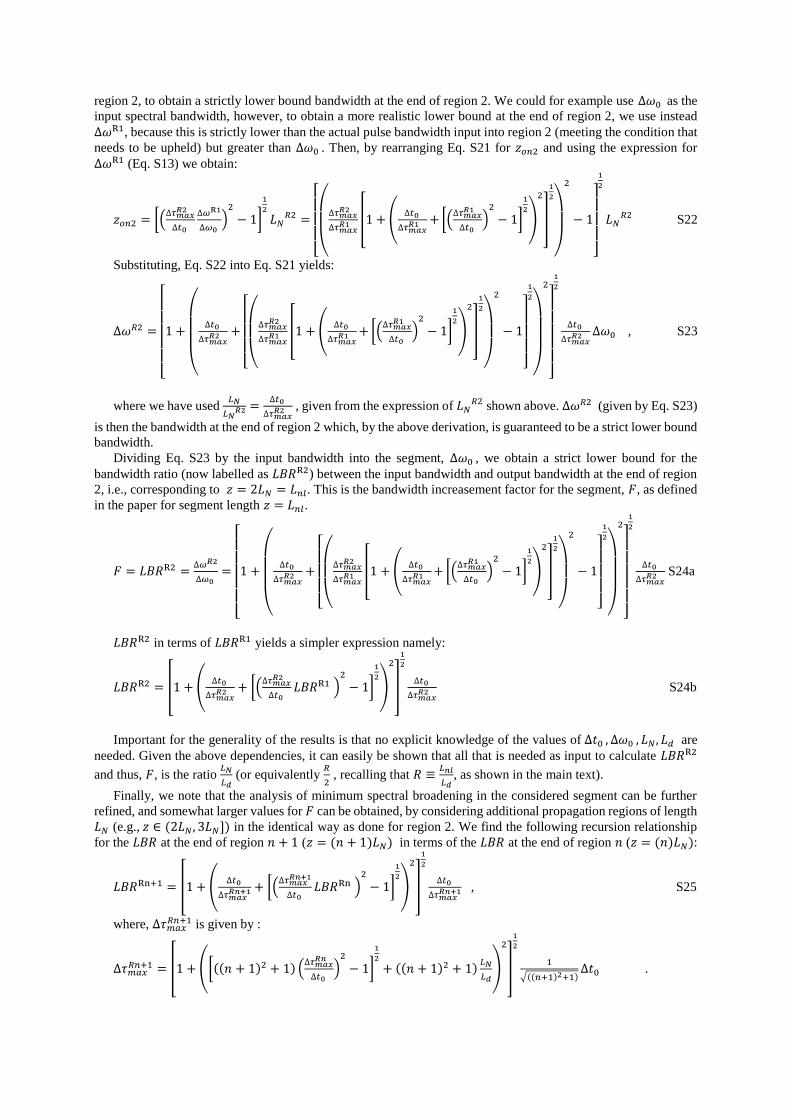
Finally, we note that the analysis of minimum spectral broadening in the considered segment can be further
refined, and somewhat larger values for 𝐹 can be obtained, by considering additional propagation regions of length
𝐿𝑁 (e.g., 𝑧 ∈ (2𝐿𝑁 , 3𝐿𝑁]) in the identical way as done for region 2. We find the following recursion relationship
for the 𝐿𝐵𝑅 at the end of region 𝑛 + 1 (𝑧 = (𝑛 + 1)𝐿𝑁) in terms of the 𝐿𝐵𝑅 at the end of region 𝑛 (𝑧 = (𝑛)𝐿𝑁):
𝐿𝐵𝑅Rn+1 = [1 + (∆𝑡0
∆𝜏𝑚𝑎𝑥𝑅𝑛+1 + [(
∆𝜏𝑚𝑎𝑥𝑅𝑛+1
∆𝑡0 𝐿𝐵𝑅Rn )
2
− 1]
1
2
)
2
]
1
2
∆𝑡0
∆𝜏𝑚𝑎𝑥𝑅𝑛+1 , S25
where, ∆𝜏𝑚𝑎𝑥𝑅𝑛+1 is given by :
∆𝜏𝑚𝑎𝑥𝑅𝑛+1 = [1 + ([((𝑛 + 1)2 + 1) (
∆𝜏𝑚𝑎𝑥𝑅𝑛
∆𝑡0 )
2
− 1]
1
2
+ ((𝑛 + 1)2 + 1)𝐿𝑁
𝐿𝑑)
2
]
1
2
1
√((𝑛+1)2+1)∆𝑡0 .

In order to provide additional insight to the dynamics of the bandwidth increasement factor, 𝐹, versus 𝑅 in
the alternating dispersion structure, we obtain the 𝑅𝑝 and 𝐹𝑝 values at every 𝑝𝑡ℎ ND segment in the numerical
alternating fiber example of Fig. 1D (numbered from ND1 to ND11) obtained from the full GNLSE under
constant 𝛽2. A plot of the 𝐹𝑝 values (solid blue curve) versus 𝑅𝑝 values is shown in Fig. S1.
For comparison, and as a proof that Eq. S24 is a lower-bound expression for the bandwidth increase in a ND
segment, we also plot the calculated 𝐹𝑝 values, using Eq. S24, for the 𝑅𝑝 values given by the numerical example.
The results of the calculation are shown as a dotted trace in Fig. S1. It can be seen that Eq. S24 displays the same
type of dependence vs. 𝑅, while remaining below the results from the numerical calculation.
Also shown in Fig. S1 is numerical proof that the 𝐹𝑝 decreases and 𝑅𝑝 increases for increasing ND segment
numbers (increasing 𝑝) in the sign-alternating dispersion structure as described in the main text.
Fig. S1. Solid trace: bandwidth increasement factor, 𝐹 versus 𝑅 of the numerical example. The specific ND segment
belonging to an (𝐹, 𝑅) pair is labelled on the graph. Dotted trace: lower bound calculation according to Eq. S24. The
latter is indeed always lower than the numerical data, but has the same type of dependence versus 𝑅.
Derivation of Main Text Eq. 2
Eq. 1 can be approximated by an exponential function shown in Eq. 2, for segments whose 𝑅 =𝐿𝑛𝑙
𝐿𝐷 ≤ 1. As a first
approximation for the base of this exponential function, in the limit (𝑅 ≪ 1), we omit dispersive effects deriving
𝐹𝑝, by substituting 𝑧 = 𝐿𝑛𝑙 = 2𝐿𝑁 into Eq. S6 to obtain:
Δ𝜔𝑛(𝑧 = 2𝐿𝑁) = [5]1
2Δ𝜔𝑛−1 S26
Tracing this to the first generating segment, we obtain: Δ𝜔𝑛(𝑧 = 2𝐿𝑁) = [5]1
2(𝑛)Δ𝜔0 . I.e., the exponential
function of Eq. 2 would then have 𝐹𝑝 = [5]1
2 as base.
However, even for segments where 𝑅 ≪ 1, the R value always increases and 𝐹𝑝 reduces, as a function of
segment number. Nevertheless, it can be shown that 𝐹𝑝 is sufficiently slowly decreasing such that Eq. 1 can still
be approximated by an exponential function with some average base (i.e., Eq. 2). The best fitting exponential
function within this range (i.e., for Eq. 2), would then be constructed by taking as base the geometrical mean of
the segment 𝐹𝑝 values [1].
We now explicitly prove that the 𝑅 range, where Eq. 1 can be approximated by Eq. 2 is 𝑅 ≤ 1, because 𝐹𝑝
reduces sufficiently slowly as a function of segment numbers located in this range. In order to do this, we
approximate Eq. 1 as an exponential function when each additional segment 𝐹𝑝 in the product is reduced
sufficiently slowly such that the bandwidth buildup due to that additional segment is not linear. We
correspondingly find the range of 𝐹𝑝 values where the growth is not linear and where it may be approximated as
exponential. This approximation works within the degree of accuracy we accept for a general understanding of our
approach. Further, the validity of this approximation is justified as it can be shown that the transitory region
between exponential spectral increase and linear occupies a small fraction of this range. Finally, the corresponding
𝑅 range matching this interval of 𝐹𝑝 values is then the range of validity of Eq. 2.
Proceeding, we prove by induction. To start, if the spectral increase is linear for two neighboring generating
segments (𝐹1, 𝐹2 , labels the 𝐹𝑝 of first, second segment), the following can be derived:
𝐹2 = 2 −1
𝐹1 S27
Then if the actual 𝐹2 (labelled as 𝐹2(𝑎𝑐𝑡𝑢𝑎𝑙)) satisfies 𝐹2
(𝑎𝑐𝑡𝑢𝑎𝑙) < 𝐹2, the growth would be greater than linear
across these two segments, which we then assume in our approximation as exponential.
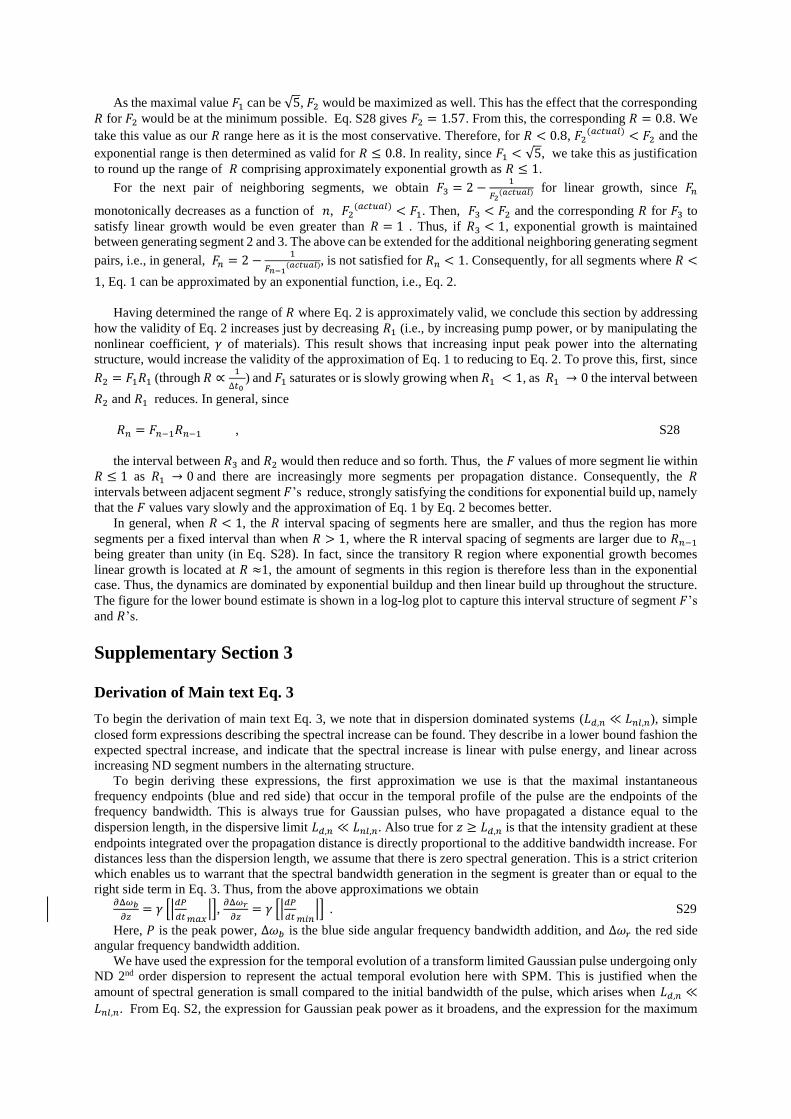
As the maximal value 𝐹1 can be √5, 𝐹2 would be maximized as well. This has the effect that the corresponding
𝑅 for 𝐹2 would be at the minimum possible. Eq. S28 gives 𝐹2 = 1.57. From this, the corresponding 𝑅 = 0.8. We
take this value as our 𝑅 range here as it is the most conservative. Therefore, for 𝑅 < 0.8, 𝐹2(𝑎𝑐𝑡𝑢𝑎𝑙) < 𝐹2 and the
exponential range is then determined as valid for 𝑅 ≤ 0.8. In reality, since 𝐹1 < √5, we take this as justification
to round up the range of 𝑅 comprising approximately exponential growth as 𝑅 ≤ 1.
For the next pair of neighboring segments, we obtain 𝐹3 = 2 −1
𝐹2(𝑎𝑐𝑡𝑢𝑎𝑙) for linear growth, since 𝐹𝑛
monotonically decreases as a function of 𝑛, 𝐹2(𝑎𝑐𝑡𝑢𝑎𝑙) < 𝐹1. Then, 𝐹3 < 𝐹2 and the corresponding 𝑅 for 𝐹3 to
satisfy linear growth would be even greater than 𝑅 = 1 . Thus, if 𝑅3 < 1, exponential growth is maintained
between generating segment 2 and 3. The above can be extended for the additional neighboring generating segment
pairs, i.e., in general, 𝐹𝑛 = 2 −1
𝐹𝑛−1(𝑎𝑐𝑡𝑢𝑎𝑙), is not satisfied for 𝑅𝑛 < 1. Consequently, for all segments where 𝑅 <
1, Eq. 1 can be approximated by an exponential function, i.e., Eq. 2.
Having determined the range of 𝑅 where Eq. 2 is approximately valid, we conclude this section by addressing
how the validity of Eq. 2 increases just by decreasing 𝑅1 (i.e., by increasing pump power, or by manipulating the
nonlinear coefficient, 𝛾 of materials). This result shows that increasing input peak power into the alternating
structure, would increase the validity of the approximation of Eq. 1 to reducing to Eq. 2. To prove this, first, since
𝑅2 = 𝐹1𝑅1 (through 𝑅 ∝1
∆𝑡0 ) and 𝐹1 saturates or is slowly growing when 𝑅1 < 1, as 𝑅1 → 0 the interval between
𝑅2 and 𝑅1 reduces. In general, since
𝑅𝑛 = 𝐹𝑛−1𝑅𝑛−1 , S28
the interval between 𝑅3 and 𝑅2 would then reduce and so forth. Thus, the 𝐹 values of more segment lie within
𝑅 ≤ 1 as 𝑅1 → 0 and there are increasingly more segments per propagation distance. Consequently, the 𝑅
intervals between adjacent segment 𝐹’s reduce, strongly satisfying the conditions for exponential build up, namely
that the 𝐹 values vary slowly and the approximation of Eq. 1 by Eq. 2 becomes better.
In general, when 𝑅 < 1, the 𝑅 interval spacing of segments here are smaller, and thus the region has more
segments per a fixed interval than when 𝑅 > 1, where the R interval spacing of segments are larger due to 𝑅𝑛−1
being greater than unity (in Eq. S28). In fact, since the transitory R region where exponential growth becomes
linear growth is located at 𝑅 ≈1, the amount of segments in this region is therefore less than in the exponential
case. Thus, the dynamics are dominated by exponential buildup and then linear build up throughout the structure.
The figure for the lower bound estimate is shown in a log-log plot to capture this interval structure of segment 𝐹’s
and 𝑅’s.
Supplementary Section 3
Derivation of Main text Eq. 3
To begin the derivation of main text Eq. 3, we note that in dispersion dominated systems (𝐿𝑑,𝑛 ≪ 𝐿𝑛𝑙,𝑛), simple
closed form expressions describing the spectral increase can be found. They describe in a lower bound fashion the
expected spectral increase, and indicate that the spectral increase is linear with pulse energy, and linear across
increasing ND segment numbers in the alternating structure.
To begin deriving these expressions, the first approximation we use is that the maximal instantaneous
frequency endpoints (blue and red side) that occur in the temporal profile of the pulse are the endpoints of the
frequency bandwidth. This is always true for Gaussian pulses, who have propagated a distance equal to the
dispersion length, in the dispersive limit 𝐿𝑑,𝑛 ≪ 𝐿𝑛𝑙,𝑛. Also true for 𝑧 ≥ 𝐿𝑑,𝑛 is that the intensity gradient at these
endpoints integrated over the propagation distance is directly proportional to the additive bandwidth increase. For
distances less than the dispersion length, we assume that there is zero spectral generation. This is a strict criterion
which enables us to warrant that the spectral bandwidth generation in the segment is greater than or equal to the
right side term in Eq. 3. Thus, from the above approximations we obtain 𝜕Δ𝜔𝑏
𝜕𝑧= 𝛾 [|
𝑑𝑃
𝑑𝑡𝑚𝑎𝑥|],
𝜕Δ𝜔𝑟
𝜕𝑧= 𝛾 [|
𝑑𝑃
𝑑𝑡𝑚𝑖𝑛|] . S29
Here, 𝑃 is the peak power, Δ𝜔𝑏 is the blue side angular frequency bandwidth addition, and Δ𝜔𝑟 the red side
angular frequency bandwidth addition.
We have used the expression for the temporal evolution of a transform limited Gaussian pulse undergoing only
ND 2nd order dispersion to represent the actual temporal evolution here with SPM. This is justified when the
amount of spectral generation is small compared to the initial bandwidth of the pulse, which arises when 𝐿𝑑,𝑛 ≪
𝐿𝑛𝑙,𝑛. From Eq. S2, the expression for Gaussian peak power as it broadens, and the expression for the maximum

absolute values for derivatives of a Gaussian function, make the temporal intensity derivatives of Eq. S29 equate
to :
|𝑑𝑃
𝑑𝑡max 𝑜𝑟 𝑚𝑖𝑛| = 𝑔𝑜
𝐸
[1+(𝑧2
𝐿𝐷2)]𝜏𝑝𝑜
2 . S30
Here, 𝐸 = √𝜋𝑃∆𝑡 is the pulse energy, 𝑔𝑜 = 0.81 is a constant related to the Gaussian pulse shape. The integral
representation of the differential Eq. S28, in the region of interest past one dispersion length is :
Δ𝜔𝑏,𝑟 = ∫ 𝛾 [|𝑑𝑃
𝑑𝑡𝑚𝑎𝑥.𝑚𝑖𝑛|] 𝑑𝑧
𝐿
𝐿𝐷 S31
We proceed by substituting Eq. S30 into Eq. S31and solving the trigonometric integral that results to obtain:
Δ𝜔𝑏,𝑟 = 𝑔𝑜𝛾2𝐸
|𝛽2|[tan−1 𝐿
𝐿𝐷−
𝜋
4] S32
Having found the bandwidth additions Δ𝜔𝑟 and Δ𝜔𝑏 for each generating segment, the total bandwidth after 𝑛
generating segments is then given as:
Δ𝜔𝑛 = Δ𝜔𝑟 + Δ𝜔𝑏 + ∆𝜔0 = 𝑛𝜋 [𝑔𝑜𝛾2𝐸
2|𝛽2|] + ∆𝜔0 S33
Its frequency representation would then be Δ𝜈𝑛 = 𝑛 [𝑔𝑜𝛾2𝐸
4|𝛽2|] + ∆𝜈0. S34
Power Scaling Laws Derivation
When 𝑃𝑂 is in the low power limit, such that 𝑅1 ≫ 1, then at the first segment, Eq. 3 applies with 𝑛 = 1 and
therefore, the growth is linear with input peak power, 𝑃𝑂 (but upper bounded by a function ∝ √𝑃𝑂) .
It is always true that 𝑅𝑛+1 > 𝑅𝑛 due to the increasing bandwidth across the ND segments of the chain, so if
𝑅1 ≫ 1 , also 𝑅𝑛 ≫ 1 is fulfilled. Under this limit, accordingly main text Eq. 3 (Eq. S33) applies for all segments
and they will scale linearly with 𝑃𝑂 (since Eq. 3 scales linearly with 𝑃𝑂 through its linear scaling with pulse energy).
Thus, Δ𝜔𝑛 = 𝑛𝜋 [𝑔𝑜𝛾2𝐸
2|𝛽2|] ∝ 𝑛𝑃𝑂 . While for the uniform dispersion waveguide, seen as one segment, Δ𝜔 ∝ 𝑃𝑂
in this limit.
As 𝑃𝑂 increases, the first segment 𝑅(1) becomes smaller than unity at some input peak power. It can be shown
that when 𝑅 < 10−1, 𝐹𝑝 at least scales close to √𝑃𝑂 here as well . Thus, we use 𝐹𝑝 ∝ √𝑃𝑂 in Eq. 2 and then the
scaling here would be: Δ𝜔𝑛 = 𝐴√𝑃𝑂 + 𝐵(𝑛 − 1)𝑃𝑂 (if only the first segment 𝑅 < 1) , where, 𝐴 > 𝐵 and are
scaling constants. As 𝑃𝑂 increases further, the approximate exponential regime is valid for an increasing number
of segments in the structure, since 𝑅 < 1 is satisfied for more segments (e.g., 𝑅1, 𝑅2, 𝑅3, 𝑒𝑡𝑐. . < 1 ). It can be
proved from the lower bound calculation that the geometrical mean (see discussion in Eq. 2 derivation section) for
the exponential function describing the spectral build-up across these segments would have base 𝐹𝑝 ∝ √𝑃𝑂 . This
continues until the bandwidth grows to high values and the linear regime applies for segments whose 𝑅 > 1.
To quantify the transition from exponential to linear growth, segment number 𝑛𝑡 labels the first segment where
𝑅 > 1. While growth for segments in the transitory region is still somewhat greater than linear (e.g. polynomial),
for the sake of simplicity we lump these segments together with the linear growth segments, making the power
scaling laws we present here a conservative estimate. In this 𝑃𝑂 power region then, Δ𝜔𝑛 = (𝐴√𝑃𝑂)𝑛𝑇−1
+
𝐵(𝑛 − 𝑛𝑇 + 1)𝑃𝑂. For a more compact expression we replace the equation with constants 𝐴, 𝐵 with a
proportionality law and represent this overall as Δ𝜔𝑛 ∝ (𝑐𝑇√𝑃𝑂)𝑛𝑇−1 + (𝑛 − 𝑛𝑇 + 1)𝑃𝑂, 𝑐𝑇 ≡𝐴
𝐵−𝑛𝑇+1 > 1.
We note that when we increase 𝑃𝑂 further, at the extreme power limits, the lower bound estimate presented
above (Δ𝜔𝑛 ∝ (𝑐𝑇√𝑃𝑂)𝑛𝑇−1 + (𝑛 − 𝑛𝑇 + 1)𝑃𝑂), must be adjusted. The reason is that at very small 𝑅 values (i.e.,
𝑅 < 10−2), the lower bound estimate would have to be extended past region 2, i.e., 𝑧𝑝 > 𝐿𝑛𝑙, because the
stagnation length now is much greater than the nonlinear length. Here, 𝐹𝑝 is ∝ √1
𝑅𝑝 for all segments in the region
𝑅 ≪ 1 (translating to 𝐹𝑝 ∝ √𝑃𝑝, where, 𝑃𝑝 is the peak power entering segment number 𝑝) as given in main text
references. This translates to a fast build up the spectrum and large relative 𝑅 jumps for subsequent segments (in
the region 𝑅 ≪ 1). It can be shown through the recursive relationships that govern 𝑅 and 𝐹𝑝 (Eq. S28) that the

following power scaling law can be derived here : Δ𝜔𝑛 = (𝐴)𝑛𝑇−1𝑃𝑂 + 𝐵(𝑛 − 𝑛𝑇 + 1)𝑃𝑂 = [𝑐𝑇𝑛𝑇−1 +
(𝑛 − 𝑛𝑇 + 1)]𝑃𝑂. Where we preserve the conservative scaling by ignoring segments within the 𝑅 range between
𝑅 ≪ 1 and 𝑅 > 1.
To give an overview, the described results are summarized in the following table of power scaling that rules
spectral broadening in the dispersion alternating structure, compared to spectral broadening in a conventional
structure with uniform dispersion.
Table S3. Overview on spectral bandwidth vs input peak power scaling laws
Regime Alternating structure
Uniform
dispersion
waveguide
𝑹𝟏 > 𝟏 Δ𝜔𝑛 ∝ 𝑛𝑃𝑜 Δ𝜔 ∝ 𝑃𝑜
𝑹𝟏 ≤ 𝟏 Δ𝜔𝑛 ∝ (𝑐𝑇√𝑃𝑂)𝑛𝑇−1 + (𝑛 − 𝑛𝑇 + 1)𝑃𝑂 Δ𝜔 ∝ 𝑃𝑜
12
𝑹𝟏 ≪ 𝟏 [𝑐𝑇𝑛𝑇−1 + (𝑛 − 𝑛𝑇 + 1)]𝑃𝑂 Δ𝜔 ∝ 𝑃𝑜
12
An interesting case arises when the generating segment is the same (i.e. comprises the same material, geometry,
with the same length or with a length up to where spectral broadening stagnates, i.e., stops increasing) as the
uniform dispersion waveguide being compared to. Then, the spectral bandwidth in the alternating structure will be
greater for any power regime, in addition to the steeper scaling.
The above power scaling laws apply where losses and third order dispersion are negligible for both ND and
AD segments. Otherwise they are valid over a restricted number of segments in the structure. However, we note
that, already at 𝑛𝑓 = 2, wider bandwidths are achieved than with conventional power scaling laws in uniform
media.
Supplementary Section 4
The full experimental splice losses, lengths and material nonlinear coefficients are listed in this section, under
table S4.
Table S4. Segment type, splice losses and length
Fiber Type &
Segment Order
Segment
Length (cm)
Splice Loss
(dB) 𝜸
1. Hi1060flex 15 5.2E − 3 W−1m
2. SMF28 10 −0.30 1.1E − 3 W−1m
3. Hi1060flex 10 −0.63 5.2E − 3 W−1m
4. SMF28 8* −0.38 1.1E − 3 W−1m
5. Hi1060flex 10 −0.64 5.2E − 3 W−1m
6. SMF28 7 −0.40 1.1E − 3 W−1m
7. Hi1060flex 15 −0.56 5.2E − 3 W−1m
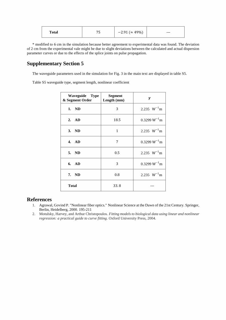
Total 75 −2.91 (≈ 49%) ---
* modified to 6 cm in the simulation because better agreement to experimental data was found. The deviation
of 2 cm from the experimental vale might be due to slight deviations between the calculated and actual dispersion
parameter curves or due to the effects of the splice joints on pulse propagation.
Supplementary Section 5
The waveguide parameters used in the simulation for Fig. 3 in the main text are displayed in table S5.
Table S5 waveguide type, segment length, nonlinear coefficient
Waveguide Type
& Segment Order
Segment
Length (mm) 𝜸
1. ND 3 2.235 W−1m
2. AD 18.5 0.3299 W−1m
3. ND 1 2.235 W−1m
4. AD 7 0.3299 W−1m
5. ND 0.5 2.235 W−1m
6. AD 3 0.3299 W−1m
7. ND 0.8 2.235 W−1m
Total 33. 8 ---
References 1. Agrawal, Govind P. "Nonlinear fiber optics." Nonlinear Science at the Dawn of the 21st Century. Springer,
Berlin, Heidelberg, 2000. 195-211
2. Motulsky, Harvey, and Arthur Christopoulos. Fitting models to biological data using linear and nonlinear
regression: a practical guide to curve fitting. Oxford University Press, 2004.