1  

SUPERMARKET ACCESS AND CHILDHOOD BODYWEIGHT:

EVIDENCE FROM STORE OPENINGS AND CLOSINGS

Di Zeng

Michael Thomsen

Rodolfo M. Nayga, Jr.

Judy Bennett

Working Paper

February 2016

2  

SUPERMARKET ACCESS AND CHILDHOOD BODYWEIGHT:

EVIDENCE FROM STORE OPENINGS AND CLOSINGS

Abstract: The food environment is increasingly hypothesized to cause obesity. This

study investigates the impacts of access to supermarkets, the primary source of healthy

foods, on the bodyweight outcomes of children. The empirical analysis uses a statewide

individual-level panel data set covering health screenings of public schoolchildren along

with annual georeferenced business lists and utilizes the plausibly exogenous variations

of supermarket openings and closings. There is little overall impact in either case, yet

supermarket openings are found to moderately reduce the bodyweight of low-income

children. These results suggest that healthy food access could help reduce childhood

obesity rates among certain population groups. (JEL Q18 I18)

3  

I. INTRODUCTION

There is a clear need for an improved understanding of childhood obesity in many

developed countries, especially the causal factors of weight gain. In the United States, nearly one

in five children is now obese (Ogden et al. 2014), facing increased health risks that extend into

adulthood (Serdula et al. 1993; Biro and Wien, 2010) as well as associated medical costs

(Trasande and Chatterjee 2009; Cawley and Meyerhoefer 2012). While scholarly investigations

have been active for decades, obesity prevalence has been inadequately explained by individual-

level factors (Garner and Wooley 1991; Cummins and Macintyre 2006). Researchers have

become increasingly aware that the complex social and physical contexts that play a role in

individual decision making could affect health outcomes (Diez-Roux 1998). The commercial

food environment, in particular, is receiving growing attention (see Walker et al. 2010; Caspi et

al. 2012 for recent reviews). It is hypothesized that access to healthy foods, or exposure to

unhealthy foods, would affect bodyweight and so the impacts of food retail outlets on

bodyweight are increasingly the topic of study. To date, studies have emphasized supermarkets

(Lopez 2007; Schafft et al. 2009; Thomsen et al. 2016), fast-food restaurants (Currie et al. 2010;

Dunn 2010; Alviola et al. 2014), and convenience stores (Morland et al. 2006; Bodor et al.

2010).

As the dominant feature of the commercial food environment, supermarkets are the most

important provider of daily foods (United States Census Bureau 2011). They are the primary

source of healthy foods such as fresh fruits and vegetables. Therefore, easy access to these stores

may contribute to better diets and lower bodyweight. For this reason, residents with limited

access to supermarkets may presumably procure a larger proportion of daily foods from

alternative food retailers such as convenience stores that carry energy-dense, less healthy foods

4  

(Morland et al. 2006). Bereft of healthy foods, these people are believed to face increased risk of

weight gain. This argument has led to concerns that some regions are “food deserts” where

limited access to supermarkets could adversely impact diet quality. Food deserts have received

increasing scholarly attention, yet empirical findings are mixed (Schafft et al. 2009; Walker et al.

2010; Caspi et al. 2012; Alviola et al. 2013, Thomsen et al. 2016).

On the other hand, it is argued that rising obesity in the United States could be a result of

reductions in real food prices that are partly induced by logistical innovations of major

supermarkets (Chou et al. 2004; Hausman and Leibtag 2007). Hence, better access to

supermarkets can be associated with lower food prices, thereby increasing food consumption and

energy intake. Evidence in favor of this argument is provided by Courtemanche and Carden

(2011), who find that Walmart Supercenters lead to increases in the bodyweight of nearby

residents. Moreover, in addition to healthy foods such as fresh fruits and vegetables,

supermarkets also stock an abundance of processed, energy-dense foods at price points lower

than most alternative food retailers, which may stimulate the consumption of such foods. In this

regard, there is empirical evidence that an increased market share of supercenters reduces

purchase healthfulness for groceries (Volpe et al. 2013).

These competing arguments suggest that the impact of supermarkets on bodyweight is

complicated and further evidence is needed to understand the linkage between the commercial

food environment and health. There have been recent calls for experimental methods and causal

evidence linking environmental factors to health outcomes (Institute of Medicine 2010).

However, such evidence is largely absent in the existing commercial food environment literature

due to data limitations. In an attempt to fill this void, we extend this literature by providing some

population-wide evidence of the weight impact of supermarkets on children. In contrast to

5  

existing studies focusing on food deserts alone (e.g., Schafft et al. 2009; Alviola et al. 2013,

Thomsen et al. 2016), we consider the broader issue of supermarket access, and identify its

causal impacts on the bodyweight of children by exploiting the plausibly exogenous variation of

store openings and closings.

This article extends a recent study by Thomsen et al. (2016) who specifically investigate

the impacts of food deserts on the bodyweight of young children (kindergarten, grades one, two

and four). They show that exposure to food deserts is positively associated with the bodyweight

of those children, but are unable to conclude causality because changes in food desert status are

mainly a result of home relocation, an endogenous event. This article differs from the Thomsen

et al. (2016) study in important ways. Instead of focusing narrowly on food deserts, which are

defined as low-income areas that lack access to supermarkets, we focus more broadly on the

issue of supermarket access and do not impose the additional neighborhood income tests.

Second, our sample is restricted to children that were in stable residential locations so that the

only source of variation in supermarket access is due to the opening or closing of a nearby

supermarket, which is plausibly exogenous to individual households.

We utilize an individual-level panel dataset that covers the body mass index (BMI)

measures of public schoolchildren in Arkansas, United States and that has been georeferenced by

year to different types of food retail establishments. As compared to Thomsen et al. (2016), our

analysis covers a much broader range of children from pre-kindergarten through grade twelve,

yet focuses on a narrower time span during which children were subject to annual as opposed to

biennial BMI screenings. The BMI measures are based on measured heights and weights and this

is a clear advantage as errors in self reporting BMI can be significant and can substantially affect

empirical findings (Cawley et al. 2015). We focus on supermarket openings and closings that

6  

affect only a portion of the population and those children that remained in stable residences,

which enables us to employ a difference-in-differences (DID) strategy to identify the causal

relationship. Two DID models are estimated. The first compares the BMI z-scores of children

who experienced supermarket openings and therefore started to have supermarket access (the

treatment group) with the BMI z-scores of children who never had access to supermarkets (the

control group). The second compares the BMI z-scores of children who experienced supermarket

closings and therefore lost supermarket access (the treatment group) with the BMI z-scores of

children who always had access to supermarkets (the control group).

We find little overall impact of supermarket openings and closings at the population

level. However, in contrast to Thomsen et al. (2016), there is evidence that supermarket openings

slightly reduce the BMI z-scores of low-income children in this broader sample. To minimize

concerns about the validity of our identification strategy, we further conduct a series of

robustness checks to rule out alternative mechanisms that could cause estimation biases. These

exercises consistently support the main results.

The rest of the article is structured as follows. Section 2 describes the data. Section 3

discusses our empirical methods. Section 4 presents baseline results as well as robustness checks.

Section 5 discusses our findings in context. Section 6 finally concludes.

II. DATA

Annual BMI screening of public schoolchildren in Arkansas started in the 2003/2004

academic year in partial fulfillment of the requirements of Act 1220, passed in 2003 by the

Arkansas General Assembly. Children were screened annually through the 2006/2007 school

year and biennially in subsequent years. The screenings are conducted by trained personnel in

7  

public schools across the state, and data are maintained by the Arkansas Center for Health

Improvement (ACHI), who worked with us to match children’s residences to the locations of

food retail establishments and to the 2009 American Community Survey (ACS) by census block

group.1 Additional information about the Arkansas BMI dataset is provided by Justus et al.

(2007) and Thomsen et al. (2016). Our analysis of these data took place on a secure computer in

ACHI’s offices in Little Rock, Arkansas.

The outcome variable of interest is the age- and gender-specific BMI z-scores computed

according to the guidelines of the United States Centers for Disease Control and Prevention. The

use of BMI z-scores rather than direct BMI values helps to control for possible confounding

factors, such as age-related adiposity rebound, puberty, and gender differences in growth

trajectories. In addition to the BMI measures, the age, gender, race, school, and school lunch

qualification (whether the child was eligible for free or reduced-price school lunch) of each child

are also present in the data.

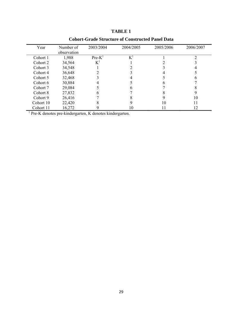
We analyze a sample covering from 2003/2004 to 2006/2007 academic years, during

which all public schoolchildren were screened annually. By restricting the sample to the

2003/2004 and 2006/2007, we are able to construct a balanced panel containing four consecutive

BMI observations per child. We further restrict the sample to only include children that were

observed in the same residential location during all four years of observation. This helps to

minimize the confounding impacts that may have given rise to home relocation decisions. The

available cohort-grade structure is depicted in Table 1.

                                                            1 Annual food store location data were obtained from Dun and Bradstreet (D&B), which are commonly used in the commercial food environment literature (e.g. Powell et al. 2007; Zick et al. 2009; Bader et al. 2010).  

8  

The accessibility of supermarkets is then defined by a binary variable indicating the

existence of a supermarket within a given radius of the residence of that child.2 The United

States Department of Agriculture (USDA) uses the cutoff of one (ten) mile(s) for urban (rural)

areas and define low-access communities as those census tracts without supermarkets within

such distances.3 This pair of radii, however, appears to be less appropriate in our finer-scale data.

Specifically, our data show that in urban areas, 21.03%, 56.93% and 86.86% of the observations

have access to supermarkets within one half mile, one mile and two miles, while in rural areas,

13.06%, 46.80% and 83.80% of the observations have access to supermarkets within two miles,

five miles and ten miles. Hence, one mile for urban areas and five miles for rural areas appear to

be best available midpoints for the sake of variation. Accordingly, we define a residential address

as one with supermarket access if the exact distance to the nearest supermarket is less than one

(five) mile(s) for urban (rural) areas, and as one without supermarket access if the distance is

larger than those cutoffs. That said, we conduct robustness checks using the USDA cutoffs.

Given the four-year study period (from 2003/2004 to 2006/2007 school years), we

specifically consider supermarket openings and closings that occurred between 2004/2005 and

2005/2006 school years, and exclude children who experienced supermarket openings or

closings in the other years during the study period. This design ensures two periods of

observation before the change in supermarket access, and another two periods of observation

after the change. The goal is to provide sufficient time for any impact of supermarket openings

or closings to manifest itself in terms of BMI z-scores. Furthermore, access to two observations

                                                            2 We define supermarkets as food stores that contain a fresh produce department. We examined the names and trade styles in the store location data to identify chain stores and affiliated grocers that provide fresh produce, and further used phone calls and Google Street-view images to verify store formats in questionable cases. 3 See http://apps.ams.usda.gov/fooddeserts/fooddeserts.aspx.

9  

prior to the change allows us to assess the parallel trend assumption essential to DID

identification, which we will further address in Section 5.

While our emphasis is on the relationship between supermarket access and childhood

bodyweight, we acknowledge that other features of the commercial food environment could also

play a role in bodyweight production. Analogous to our measurement of supermarket access, we

further account for access to convenience stores and fast-food restaurants around the residence of

each child. A dummy access indicator for each type of store is based on a half mile radius for

urban residences and a two mile radius for rural residences because these are the best available

midpoints for variation. Formal consideration of these additional store types will also be

discussed in Section 5.

Table 2 presents the summary statistics for our samples. Between the 2004/2005 and

2005/2006 school years, supermarket openings resulted in the reclassification of 1,064 children

that previously had no supermarket access, while supermarket closings resulted in the

reclassification of 1,210 children that previously had access to a nearby supermarket to no

access. The pairwise t-tests suggest that there are few statistical differences in the average BMI

z-scores by treatment status. In comparison to the control group, children who experienced

supermarket openings or closings are less likely to qualify for free school lunch and are less

likely to be of Hispanic ethnicity. Moreover, children who experienced supermarket openings are

more likely to be from more affluent communities than children who never had supermarket

access, while children who experienced supermarket closings are more likely to be from less

affluent communities and rural communities than children who always had supermarket access.

Despite statistical significance, most of these differences are small in magnitude, implying that

the children have fairly similar characteristics regardless of treatment status.

10  

III. ANALYTICAL FRAMEWORK

Two DID models are estimated using the supermarket access measure for each child.

First, we compare the BMI z-scores of children who were affected by supermarket openings, and

therefore started to have supermarket access, to those of children who never had access to nearby

supermarkets during the study period. Second, we compare the BMI z-scores of children who

were affected by supermarket closings, and therefore lost access to a nearby supermarket, to

those of children who always had access to nearby supermarkets during the study period.

According to our data, supermarket openings and closings that change the store access status

almost always involved only one supermarket.4

A. Identification Strategy

In either the case of supermarket openings or closings, the baseline DID regression model

can be specified as:

(1)

where is the weight outcome of child in school year , measured by BMI z-score. is a

binary indicator of the treatment status, which equals one if child belongs to the treatment

group, or zero if he/she belongs to the control group. is a binary indicator of the timing of

observation, which equals one for post-treatment observations, or zero for pre-treatment

observations. is a vector of covariates, and is the idiosyncratic error. In the empirical

estimation, includes the age, gender, whether the child qualifies for free school lunch, and

two dummy variables indicating whether the child is African American or of Hispanic ethnicity.                                                             4 The opening or closing of a supermarket around the residence of the child would not affect his/her access status if an alternative supermarket was also accessible. The openings or closings of multiple supermarkets at the same time are very rare.

11  

The coefficient of primary interest is , which identifies the respective impact of

supermarket openings and closings. Empirical estimates of , however, can be underestimated

since households without nearby access to supermarkets in the given radii may still purchase

foods from supermarkets at a longer distance, which may attenuate any possible impacts. This

gives rise to a broader issue concerning the intensity of treatment, where the behavioral

responses of households induced by the openings or closings of a supermarket can be less

meaningful if alternative supermarkets are also accessible with only minor changes in travel

distance and/or travel time.5 To address this, we extend the baseline models and consider two

additional analyses where the treatment group is restricted to children who observed supermarket

openings or closings that involved the only available supermarket within larger radii of two miles

(urban) and ten miles (rural), while keeping the control group the same (this is referenced

hereafter as the “extended model”). This design would largely control for possible confounding

impacts from alternative supermarkets and therefore reduce the downward estimation biases.

Since we have four rounds of observations for each child, the empirical estimation of Eq.

(1) is subject to serial correlations that can result in estimation bias, which needs to be formally

addressed. Several possible empirical strategies to correct for serial correlations are discussed in

Bertrand et al. (2004), including block-bootstrap error correction, arbitrary variance-covariance

matrix correction, empirical variance-covariance matrix correction, and aggregating the time

series information. In a series of Monte Carlo simulations with placebo treatments inserted into

real data, Bertrand et al. (2004) further show that all these methods perform well if the number of

groups (i.e. clusters of individuals that observe the same policy treatment) is sufficiently large,

                                                            5 In fact, we have also examined cases where the opening or closing of supermarkets do not change the access status of children. Specifically, we investigated whether the increases or decreases in the number of accessible supermarkets, occurring between 2004/2005 and 2005/2006 school years, would affect BMI z-scores. However, we find little evidence that these changes in the number of stores matter.  

12  

while only the last method performs satisfactorily for a small number of groups. Unlike many

policy interventions targeted at certain regions, the “groups” are difficult to define in our case

because there is no natural cluster within the treatment and control groups. Even children in the

same community might have different treatment status because the exact distance from each

residence to the nearest supermarket utilized that we use in the analysis varies across households.

We therefore opt to aggregate the time series information to correct for serial correlation over

time. Specifically, we average the data before and after the treatment and estimate Eq. (1) on the

averaged BMI z-scores in a panel of length two.6

B. Treatment exogeneity

The estimate of can be interpreted as causal if two identification assumptions hold.

First, the openings and closings of supermarkets are exogenously determined for each household

and therefore each child (treatment exogeneity). Second, the counterfactual trend in the BMI z-

scores of the treated children, were the treatment not received, would have been the same as the

untreated children (the parallel trend assumption). Although we will empirically test the parallel

trend assumption in Section 5, treatment exogeneity is not directly testable, and is worth some

more discussion.

At the household level, it is unlikely that any single household is important enough to

meaningfully affect store locations. Moreover, few households possess sufficient foreknowledge

of future supermarket openings or closings that could factor into their residential location

decisions. Therefore, treatment exogeneity at the household level should be reasonably satisfied.

Still, there is a possibility that residents from a community could exhibit some common features

                                                            6 Impact results are dubiously more statistically significant without the aggregation of the time series information. This pattern is discussed in Bertrand et al. (2014) as a result of underestimated standard errors of the DID estimator.  

13  

that result in both supermarket opening/closing and weight changes of children. It could

specifically be the case if the opening/closing of a supermarket occurs as a result of

catering/failure to cater the specific food preferences of consumers in certain communities. To

minimize this concern, we re-estimate Eq. (1) using a series of homogenized subsamples that

may maintain different consumption behaviors. Specifically, we assess samples homogenized by

neighborhood income, vehicle ownership status, and urbanity.

We subsample by income because income is an important socioeconomic indicator and

low income is a feature of food deserts (Lopez 2007; Schafft et al. 2009; Thomsen et al. 2016).

Therefore, we consider the median household income of each census-block group (from 2009

ACS), and define low (high) income communities as census-block groups with median

household incomes below (above) the statewide median income. We also evaluate community

economic situation using vehicle ownership rate, as the distance to supermarkets may be more of

an issue for households without a vehicle (Fitzpatrick et al. 2016). The proportion of residents

without vehicles are also retrieved from the 2009 ACS, and the full sample is broken into two

subgroups divided by the statewide median vehicle ownership rate. We further differentiate

children living in rural and urban residences, as rural and urban households may exhibit varying

food procurement practices as well as differences in vehicle dependence.

The subsample estimations will then help control for the remaining endogeneity, if any,

at the community level. They also serve the dual purpose of testing any impact heterogeneity

among different population groups. In Section 5, we further apply alternative DID regression as

well as matching methods to establish our main results, which jointly lend credence to the

plausibility of treatment exogeneity.

14  

IV. BASELINE RESULTS

Table 3 presents the BMI impact estimates of supermarket openings and closings for all

children as well as different subsamples. All children in the full sample are assigned to

subsample classified by neighborhood income, vehicle ownership rate, and urbanity. Robust

standard errors are reported in each case.

At the population level, the overall impacts are small and statistically insignificant, but

the subsample estimates do exhibit some interesting patterns. Specifically, supermarket openings

are found to significantly reduce the BMI z-scores of children from communities with low

household income and low vehicle ownership rates, or the low-income children in general (as

these two subsamples largely overlap). In the baseline model, a new supermarket reduces the

BMI z-scores of low-income children by 0.090-0.096 standard deviations. The extended model

further confirms this impact, yielding slightly larger estimates. These findings provide some

support to the argument that better access to supermarkets (and therefore healthy foods) may

reduce the bodyweight of children. It is possible that the nearby supermarket openings could

have substantially shifted the food purchase and consumption patterns of the low-income

population towards healthy foods, and therefore reduced the bodyweight of children.

Unlike the subsample impacts of supermarket openings, few subsamples show significant

impacts of supermarket closings. The only exception is that in the extended model, supermarket

closings lead to an increase of BMI z-score by 0.044 standard deviations for low-income

children. Nevertheless, this impact is nonexistent in the baseline model. We speculate that,

unlike the opening of a new supermarket that can induce an increase in demand for relatively

healthier food given the improved shopping convenience, the closing of an existing supermarket

15  

may less likely alter established food purchasing patterns, especially those based on food

traditions, tastes and preferences of food healthfulness.

In sum, although the overall BMI impacts of supermarket openings or closings are small

and statistically insignificant, there is evidence that supermarket access matters among low-

income children. These findings imply that healthy food access could contribute to bodyweight

reduction. We now turn to robustness check procedures to further establish the validity of these

estimates.

V. ROBUSTNESS CHECKS

In addition to subsample estimation, we further apply two strategies to address concerns

about endogeneity of supermarket openings and closings. In the first strategy, we estimate our

baseline model and extended model with an alternative DID specification augmented by

community and year fixed effects. The community fixed effects control for unobserved time-

invariant community characteristics (e.g. similar lifestyles). The year fixed effects further takes

into account any macroeconomic dynamics that could affect the bodyweight of children (e.g.

changes in employment opportunities). The augmented DID regression model is specified as:

(2)

where is the community fixed effects and is the year fixed effects, with other terms defined

in Eq. (1). Concerns about any systematic differences among communities that could have

contributed to the estimated BMI impacts should be minimized if our main results can be

replicated by the estimation of Eq. (2).

In the second strategy, we alternatively use difference-in-differences matching (DID

matching) techniques to estimate the impacts of supermarket openings and closings. The DID

16  

matching estimator compares the conditional before-after outcomes of the treatment group with

those of the control group (Heckman et al. 1997). It relaxes the linear functional form required in

regression, and it re-weights the observations in the control group using semiparametric methods

(Smith and Todd 2005). Changes in BMI z-scores before and after the treatment are then

matched using a set of observed characteristics. Using subscripts ′ and to denote the

(aggregated) before-treatment period and after-treatment period, the DID matching estimator is

computed as:

(3) ∆ ∑ Ε |Ρr , 0 ∑ Ε |Ρr , 0

where the superscript 1 or 0 indicates that child belongs to the treatment group or control

group, respectively; Ε ∙ is a nonparametric weighting function that can be estimated with

matching methods such as nearest neighbor or kernel density; and Ρr ∙ is the propensity score

function which estimates the probability that child observes either supermarket opening or

closing based on observed characteristics. We specifically consider propensity score matching

because it is equivalent to directly matching observed characteristics in all their dimensions

while it avoids the curse of dimensionality that prevents successful matching (Rosenbaum and

Rubin 1983). Under the identification assumption that the BMI z-scores of children are

independent of supermarket openings or closings conditional on the observed characteristics, the

DID matching estimator unbiasedly identifies the average treatment effect on the treated. If

supermarket openings and closings can be considered as random, it further identifies the

population average treatment effect. Therefore, DID matching should be able to replicate our

regression-based impact estimates if treatment exogeneity actually holds (i.e. unobservables do

not affect treatment status).

17  

Table 4 presents the impact estimates from these procedures, namely alternative DID

regressions with community and year fixed effects, DID nearest neighbor matching and DID

kernel matching for a total of three procedures. In general, these estimates are very similar to our

main results in terms of impact magnitudes and statistical significance. There is little impact at

the population level. For supermarket openings, it is seen again that improvements in store

access reduce the BMI z-scores of low-income children. In the extended model, even the overall

impact estimated by DID nearest neighbor matching is statistically significant at the 5% level

(middle panel). In a few cases, the impacts on children from communities with low vehicle

ownership rates lose statistical significance at the 5% level (upper and lower panels), but their

magnitudes change little and both remain significant at 10% level. On the other hand, the

impacts of supermarket closings again appears to be less robust. Despite the few discrepancies,

the results suggest that there is little evidence against treatment exogeneity, providing fairly

strong support to our main results.

The second threat to the validity of our results concerns whether the parallel trend

assumption is satisfied, which is essential to DID regression identification. The parallel trend

assumption asserts that the counterfactual trend in the BMI z-scores of children who observed

supermarket openings (closings) would have been the same as the children who never (always)

had supermarket access had there not been supermarket openings (closings). Violation of this

assumption can lead to biased estimates, which might have resulted from the intrinsic differences

that could have produced different BMI trends of children in the treatment and control groups

over time rather than from supermarket openings or closings felt by the children in the treatment

group.

18  

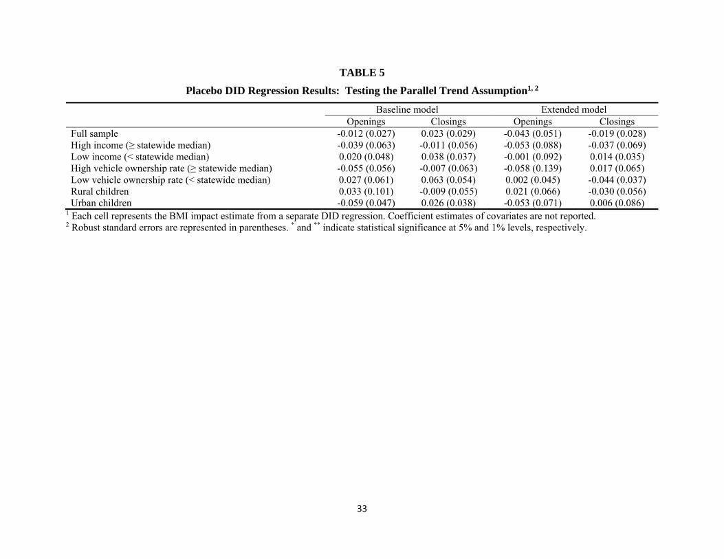
We assess the validity of the parallel trend assumption through the performance of

placebo DID regressions with the two rounds of observations, namely 2003/2004 and 2004/2005

school years, before the supermarket openings or closings that we consider (between 2004/2005

and 2005/2006 school years). Without time series aggregation (as applied to our main DID

regressions), this pre-treatment panel provides richer information about any possible

discrepancies in BMI trends before treatment and control groups. Each placebo DID regression is

specified exactly the same as in Eq. (1), while we consider a placebo treatment between

2003/2004 and 2004/2005 school years to the children in the real treatment group who finally

observed such changes a year later, and redo the analysis. Since our samples do not include

supermarket openings and closings between these two years by construction, the DID interaction

terms should be zero. Statistical significance in these placebo DID regressions, if any, would

imply the violation of the parallel trends assumption. Impact estimates are presented in Table 5.

In all cases, we see no statistically significant difference between the BMI z-scores between

children in the treatment and control groups, suggesting that the parallel trend assumption is

reasonably satisfied, and lending credence to our identification strategy and main results.

We further perform two additional robustness exercises to check the possible existence of

alternative mechanisms that could have contributed to the above estimated BMI impacts. The

first procedure investigates possible confounding impacts of the school food environment.

School meals are an important food source for youth, and possible differences across schools

may confound the estimated impacts of supermarket openings and closings. To address this

issue, we estimate an alternative DID regression model which is similar to that specified in Eq.

(2) but is now augmented by school and grade fixed effects instead of community and year fixed

effects, in hope of capturing any time-invariant heterogeneity in school food practices.

19  

In addition to supermarkets, other features of the commercial food environment could

also play an unrecognized role in affecting the bodyweight of children. We formally control for

access to convenience stores and fast food restaurants as both have received growing attention in

recent literature (e.g. Morland et al. 2006; Dunn 2010; Alviola et al. 2014). Similar to the

supermarket access measure, we construct two binary access indicators that equals one if there

exist(s) one or more stores of either type within a half-mile (two-mile) radius in an urban (rural)

setting. These cutoffs are the best available midpoints that allow maximal variation in the store

access measures in both cases. They enter Eq. (1) as additional covariates which vary not only

across individuals but also over time (with the openings and closings of these stores as the source

of variation).

Table 6 reports the impact estimates from these two procedures. Most estimates with

statistical significance are also numerically close to our main results. Although the impact of

supermarket openings on children from communities with low vehicle ownership rates loses

statistical significance at the 5% level in the baseline model estimation, there are only trivial

changes in their magnitudes and both estimates are still significant at the 10% level. The impacts

of supermarket openings in the extended model exhibit even higher similarities to our main

findings. On the other hand, the impacts of supermarket closings are less robust.

The final robustness check concerns the distance used to define supermarket access. As

noted above, our definition of supermarket access differs from that of USDA where residences

one (ten) mile(s) away from the nearest supermarket in an urban (rural) area are labeled as low

access. We further check if our results hold with an alternative supermarket access measure

defined using the USDA radius cutoffs. Table 7 presents the impact estimates. Although the

magnitudes of most estimates with statistical significance are much smaller than our main

20  

results, they still appear to be consistent enough to our main results, especially with greatly

reduced variation in the supermarket access measure.

VI. DISCUSSION

We find little overall impact of supermarket access on the bodyweight of children.

However, at the subsample level, supermarket openings are found to have small weight-reducing

impacts for low-income children as measured by both community-level income status and

vehicle ownership rates. These results hold across a series of robustness checks, and consistently

suggest that appropriate access to healthy foods does play a desirable role in the bodyweight

production of these children.

Further insights can be obtained by placing the significant subsample impacts in context.

Our main results suggest that supermarket openings can reduce BMI-z-scores for low-income

children by 0.090 to 0.096 standard deviations. Consider a boy of 11.5 years (138 months, which

is close to the average age of our full sample). A boy 4 feet 10 inches in height with a weight of

92.5 pounds would have a BMI z-score of 0.684, which is near our sample average. A decrease

in BMI z-score of 0.090-0.096 standard deviations would translate into a weight reduction of

roughly 1.3 to 1.4 pounds with no change in height. Therefore, the BMI impacts are not large in

terms of bodyweight, especially given the prominent role of supermarkets in the commercial

food environment.

Going into this study, we do not have strong a priori hypotheses on the signs of the BMI

impacts of supermarket openings and closings. On one hand, appropriate access to supermarkets

may reduce bodyweight by providing access to healthy foods. On the other hand, lower price

points and the abundance of unhealthy foods in large package sizes in supermarkets could

21  

contribute to increases in bodyweight. These mechanisms could come into play simultaneously;

hence our estimates could be the net impacts of multiple conflicting mechanisms. While our

analysis does not directly address these possible underlying mechanisms (which is neither within

the scope of the study nor feasible given our current data), our subsample results suggest that

access to healthy foods can matter more on balance. Moreover, since our primary finding is

mainly about the desirable impacts of supermarket openings, these estimates are likely the lower

bounds of the true impacts because the alternative mechanisms regarding income effects and

provision of unhealthy foods in supermarkets would unambiguously increase bodyweight, and

thus could possibly offset the true impacts of supermarket openings.

It is noteworthy that most consistent findings come from the subsample of lower-income

children. This is in contrast to Thomsen et al. (2016) who found no BMI impact among children

switching out of food deserts by reason of supermarket openings. Although our estimated BMI

impacts are small, they are still important given the vulnerability of these children. National-

level evidence shows that from 2003 to 2007, obesity prevalence increased by 10% for all

children in the United States but increased by 23% for children from low-income households

(Singh et al. 2010). In another nationally representative sample, the rates of severe obesity were

approximately 1.7 times higher among poor children and adolescents aged 2 to 19 years (Skelton

et al. 2009). Low-income communities are often food deserts (Beaulac et al. 2009), where

available healthy foods are more expensive (Drewnowski 2010), and are of poorer quality

(Andreyeva et al. 2008). It is for these reasons that these communities are increasingly found to

observe higher childhood obesity rates (Lopez 2007; Schafft et al. 2009; Ghosh-Dastidar et al.

2014). Regarding supermarket openings, there is evidence that new supermarket entries and

increased supermarket competition reduce food prices (Basker and Noel 2009), and improve

22  

food quality (Matsa 2011). On the food demand side, it is further found that supermarket access

is associated with increased daily consumption of fruits and vegetables among food stamp

recipients (Rose and Richards 2004). Hence, improvements in supermarket access in low-income

communities could enhance healthy food access in all these aspects, which could then potentially

reduce the bodyweight of children in those communities.

Despite the moderate magnitudes of BMI impacts on low-income children, they still

provide some reliable information for policy decisions. There is no simple answer to dealing

with childhood obesity, which is certainly a joint product of numerous factors. Admittedly,

access to healthy foods is only one possible factor that could affect the bodyweight of children.

That said, our study does confirm its role for low-income children, who are among the neediest

members of society for health improvement.

VII. CONCLUDING REMARKS

We investigate the possible relationship between supermarket access and childhood

bodyweight using the plausible exogenous variation of supermarket openings and closings. At

the population level, we see little evidence that supermarket access affects the BMI z-scores of

children. However, supermarket openings are found to have moderate weight-reducing impacts

on low-income children. Such impacts are highly significant and robust across a series of

robustness checks. The estimated BMI impacts finally translate into a one or two pound

bodyweight reduction which, though not large, is likely a conservative estimate and still of

policy significance when specifically felt by low-income children.

Our findings that improvements in healthy food access may have desirable impacts on the

bodyweight of low-income children further justify the consideration of the commercial food

23  

environment as an added dimension in public policy designs for childhood obesity prevention.

However, as the benefits may not be equally shared among different socioeconomic groups, we

do not directly see the cost effectiveness of broadly stimulating new supermarket operations

from the social welfare perspective. Rather, our results could point to the need for better access

to healthy foods specifically targeting low-income children. Also, educational interventions

targeting both children and parents should keep receiving policy attention, especially for low-

income communities and those with larger presence of young children. While our findings do not

speak directly to the merits of these strategies, they could still contribute to more informed policy

decisions.

As one of the first studies assessing the weight impacts of supermarket access on

children, our study has several limitations. Given data constraints, we are only able to estimate

the net impacts and are unable to disentangle the possible confounding mechanisms of

supermarket access. We are also prevented from assessing impact heterogeneity among

racial/ethnic groups given their limited presence in the treatment groups. That said, we do

provide some reliable findings that supermarket access does matter for certain vulnerable

children. Moreover, given that real economic experiments are hardly feasible in commercial food

environment research, quasi-experimental methods including those applied in the current

analysis should be further encouraged. In this sense, our investigation could serve as a baseline

study that welcomes continued investigations with extensions.

24  

References

Alviola, P.A. IV., R.M. Nayga, Jr., and M.R. Thomsen. “Food deserts and childhood obesity.”

Applied Economic Perspectives and Policy, 35, 2013, 106-24.

Alviola, P.A. IV, R.M. Nayga, Jr., M.R. Thomsen, D. Danforth, and J. Smartt. “The effect of

fast-food restaurants on childhood obesity: a school level analysis.” Economics & Human

Biology, 12, 2014, 110-19.

Andreyeva, T., D.M. Blumenthal, M.B. Schwartz, M.W. Long, and K.D. Brownell. “Availability

and prices of foods across stores and neighborhoods: the case of New Haven,

Connecticut.” Health Affairs, 27(5), 2008, 1381-88.

Bader, M.D.M., M. Purciel, P. Yousefzadeh, and K.M. Neckerman. “Disparities in neighborhood

food environments: implications of measurement strategies.” Economic Geography,

86(4), 2010, 409-30.

Basker, E., and M. Noel. “The evolving food chain: competitive effects of Wal‐Mart's entry into

the supermarket industry.” Journal of Economics & Management Strategy, 18(4), 2009,

977-1009.

Beaulac, J., E. Kristjansson, and S. Cummins. “A systematic review of food deserts, 1966-2007.”

Preventing Chronic Disease, 6(3), 2009, A105.

Bertrand, M., E. Duflo, and S. Mullainathan. “How much should we trust differences-in-

differences estimates?” Quarterly Journal of Economics, 119(1), 2004, 249-75.

Biro, F.M., and M. Wien. “Childhood obesity and adult morbidities.” American Journal of

Clinical Nutrition, 91(5), 2010, 1499S-505S.

25  

Bodor, J.N., J.C. Rice, T.A. Farley, C.M. Swalm, and D. Rose. “The association between obesity

and urban food environments.” Journal of Urban Health: Bulletin of the New York

Academy of Medicine, 87(5), 2010, 771-81.

Caspi, C.E., G. Sorensen, S.V. Subramanian, and I. Kawachi. “The local food environment and

diet: a systematic review.” Health & Place, 18(5), 2012, 1172-87.

Cawley, J., and C. Meyerhoefer. “The medical care costs of obesity: an instrumental variables

approach.” Journal of Health Economics, 31(1); 2012, 219-30.

Cawley, J., J.C. Maclean, M. Hammer, and N. Wintfeld. “Reporting error in weight and its

implications for bias in economic models.” Economics & Human Biology, 19, 2015, 27-

44.

Chou, S., M. Grossman, and H. Saffer. “An economic analysis of adult obesity: results from the

behavioral risk factor surveillance system.” Journal of Health Economics, 23, 2004, 565-

87.

Courtemanche, C., and A. Carden. “Supersizing supercenters? The impact of Walmart

Supercenters on body mass index and obesity.” Journal of Urban Economics, 69, 2011,

165-81.

Cummins, S., and S. Macintyre. “Food environments and obesity - neighbourhood or nation?”

International Journal of Epidemiology, 35, 2006, 100-4.

Currie, J., S. Della Vigna, E. Moretti, and S. Pathania. “The effect of fast-food restaurants on

obesity and weight gain.” American Economic Journal: Economic Policy, 2(3), 2010, 32-

63.

Diez-Roux, A.V. “Bringing context back into epidemiology: variables and fallacies in multilevel

analysis.” American Journal of Public Health 88(2), 1998, 216-22.

26  

Drewnowski, A. “The cost of US foods as related to their nutritive value.” American Journal of

Clinical Nutrition, 92(5), 2010, 1181-88.

Dunn, R.A. “Obesity and the availability of fast-food: an analysis by gender, race and residential

location.” American Journal of Agricultural Economics, 92(4), 2010, 1149-64.

Fitzpatrick, K., N. Greenhalgh-Stanley, and M. Ver Ploeg. “The impact of food deserts on food

insufficiency and SNAP participation among the elderly.” American Journal of

Agricultural Economics, 98(1), 2015, 19-40.

Garner, D.M., and S.C. Wooley. “Confronting the failure of behavioral and dietary treatments for

obesity.” Clinical Psychology Review, 11, 1991, 729-80.

Ghosh-Dastidar, B., D. Cohen, G. Hunter, S.N. Zenk, C. Huang, R. Beckman, and T. Dubowitz.

“Distance to store, food prices, and obesity in urban food deserts.” American Journal of

Preventative Medicine, 47(5), 2014, 587-95.

Hausman, J., and E. Leibtag. “Consumer benefits from increased competition in shopping

outlets: measuring the effect of Wal-Mart.” Journal of Applied Econometrics, 22 (7),

2007, 1157-77.

Heckman, J.J., H. Ichimura, and P.E. “Todd. Matching as an econometric evaluation estimator:

evidence from evaluating a job training programme.” Review of Economic Studies, 64(4),

1997, 605-54.

Institute of Medicine. Bridging the Evidence Gap in Obesity Prevention: A Framework to Inform

Decision Making. Washington DC: The National Academies Press, 2010.

Justus, M.B., K.W. Ryan, J. Rockenbach, C. Katterapalli, and P. Card‐Higginson. “Lessons

learned while implementing a legislated school policy: body mass index assessments

27  

among Arkansas’s public school students.” Journal of School Health, 77(10), 2007, 706-

13.

Lopez, R P. “Neighborhood risk factors for obesity.” Obesity, 15(8), 2007, 2111-19.

Matsa, D.A. “Competition and product quality in the supermarket industry.” Quarterly Journal

of Economics, 126 (3), 2011, 1539-91.

Morland, K., A.V. Diez Roux, and S. Wing. “Supermarkets, other food stores, and obesity: the

atherosclerosis risk in communities study.” American Journal of Preventative Medicine,

30(4), 2006, 333–39.

Ogden, C., M.D. Carroll, B.K. Kit, and K.M. Flegal. “Prevalence of childhood and adult obesity

in the United States.” Journal of American Medical Association, 311(8), 2014, 806-14.

Powell, L.M., S. Slater, D. Mirtcheva, Y. Bao, and F.J. Chaloupka. “Food store availability and

neighborhood characteristics in the United States.” Preventive Medicine, 44(3), 2007,

189-95.

Rose, D., and R. Richards. “Food store access and household fruit and vegetable use among

participants in the US Food Stamp Program.” Public Health Nutrition, 7(8), 2004, 1081-

88.

Rosenbaum, P.R., and D.B. Rubin. “The central role of the propensity score in observational

studies for causal effects.” Biometrika, 70(1), 1983, 41-55.

Schafft, K.A., E.B. Jensen, and C.C. Hinrichs. “Food deserts and overweight schoolchildren:

evidence from Pennsylvania.” Rural Sociology, 74(2), 2009, 153-77.

Serdula, M.K., D. Ivery, R.J. Coates, D.S. Freedman, D.F. Williamson, and T. Byers. “Do obese

children become obese adults? A review of the literature.” Preventive Medicine, 22(2),

1993, 167-77.

28  

Singh, G.K., M. Siahpush, M.D. Kogan. “Rising social inequalities in US childhood obesity,

2003-2007.” Annals of Epidemiology, 20(1), 2010, 40-52.

Skelton, J.A., S.R. Cook, P. Auinger, J.D. Klein, and S.E. Barlow. “Prevalence and trends of

severe obesity among U.S. children and adolescents.” Academic Pediatrics, 9(5), 2009,

322-29.

Smith, J.A., and P.E. Todd. “Does matching overcome LaLonde’s critique of nonexperimental

estimators?” Journal of Econometrics, 125, 2005, 305-53.

Thomsen, M.R., R.M. Nayga, Jr., P.A. Alviola, IV, and H.L. Rouse. “The effect of food deserts

on the body mass index of elementary schoolchildren.” American Journal of Agricultural

Economics, 98(1), 2016, 1-18.

Trasande, L., and S. Chatterjee. “The impact of obesity on health service utilization and costs in

childhood.” Obesity, 17(9), 2009, 1749-54.

United States Census Bureau. Annual Retail Trade Report. Washington DC: United States

Census Bureau, 2011.

Volpe, R., A. Okrent, and E. Leibtag. “The effect of supercenter-format stores on the

healthfulness of consumers’ grocery purchases.” American Journal of Agricultural

Economics, 95 (3), 2013, 568–89.

Walker, R.E., C.R. Keane, J.G. Burke. “Disparities and access to healthy food in the United

States: a review of food deserts literature.” Health & Place, 16, 2010, 876-84.

Zick, C.D., K.R. Smith, J.X. Fan, B.B. Brown, I. Yamada, and L. Kowaleski-Jones. “Running to

the store? The relationship between neighbourhood environments and the risk of

obesity.” Social Science & Medicine, 69(10), 2009; 1493-500.

29  

TABLE 1

Cohort-Grade Structure of Constructed Panel Data

Year Number of observation

2003/2004 2004/2005 2005/2006 2006/2007

Cohort 1 1,988 Pre-K1 K1 1 2 Cohort 2 34,564 K1 1 2 3 Cohort 3 34,548 1 2 3 4 Cohort 4 36,648 2 3 4 5 Cohort 5 32,468 3 4 5 6 Cohort 6 30,884 4 5 6 7 Cohort 7 29,084 5 6 7 8 Cohort 8 27,832 6 7 8 9 Cohort 9 26,416 7 8 9 10

Cohort 10 22,420 8 9 10 11 Cohort 11 16,272 9 10 11 12

1 Pre-K denotes pre-kindergarten, K denotes kindergarten.

30  

TABLE 2

Summary Statistics1

All observations Supermarket opening analysis sample Supermarket closing analysis sample

(n=293,124)3 Treatment group2

(n=4,256)3 Control group2 (n=126,836)3

Treatment group2 (n=4,840)3

Control group2 (n=143,144)3

BMI z-score 0.684

(1.042) 0.671

(1.051) 0.694

(1.061) 0.688

(1.047) 0.678

(1.064)

Age (month) 137.874 (33.962)

135.672 (34.905)

137.835 (36.718)

137.463 (34.460)

137.986 (36.969)

Gender (male=1; female=0) 0.519

(0.500) 0.511

(0.500) 0.524

(0.499) 0.521

(0.500) 0.514

(0.500)

Free lunch (qualified=1; otherwise=0) 0.322

(0.424) 0.297

(0.429) 0.313 * (0.452)

0.305 (0.464)

0.331 ** (0.480)

African American (dummy indicator) 0.135

(0.318) 0.146

(0.353) 0.137

(0.341) 0.125

(0.319) 0.133

(0.435)

Hispanic (dummy indicator) 0.044

(0.163) 0.035

(0.157) 0.042 * (0.202)

0.033 (0.180)

0.049 ** (0.254)

Median household income (thousand USD)4 42.443

(15.221) 43.231

(17.299) 41.844 ** (15.143)

41.548 (14.416)

42.903 ** (17.912)

Median vehicle ownership rate (%)4 93.814 (5.032)

95.487 (5.146)

95.029 (6.192)

90.819 (5.458)

92.641 ** (8.725)

Rural residence (dummy indicator)5 0.433

(0.418) 0.436

(0.442) 0.447

(0.425) 0.455

(0.437) 0.421 ** (0.422)

1 All measures are averaged over the four years of study. Standard deviations are represented in parentheses. * and ** indicate statistical significance at 5% and 1% levels, respectively, from pairwise t-tests between treatment and control groups within each subsample. 2 The treatment group in the supermarket opening analysis subsample consists of children who had no supermarket access in the first two periods of observation while gained such access in the last two periods of observation due to supermarket openings. The control group in the supermarket closing analysis subsample consists of children who never had supermarket access during the study period. The treatment group in subsample 2 consists of children who previously had supermarket access in the first two periods of observation while lost such access in the last two periods of observation due to supermarket closings. The control group in subsample 2 consists of children who always had supermarket access during the study period. 3 The number of children is one fourth the number of observations presented here as each children is observed in four consecutive years. 4 These census-block group level statistics are from the 2009 ACS. 5 Rural-urban classification are based on 2009 ACS.

31  

TABLE 3

Baseline BMI Impact Estimates of Supermarket Openings and Closings1, 2

Baseline model Extended model Openings Closings Openings Closings Full sample -0.038 (0.032) 0.001 (0.030) -0.051 (0.031) 0.004 (0.027) High income (≥ statewide median) -0.024 (0.056) -0.003 (0.044) -0.029 (0.043) -0.015 (0.058) Low income (< statewide median) -0.096 (0.034) ** -0.021 (0.034) -0.113 (0.036) ** 0.044 (0.021) * High vehicle ownership rate (≥ statewide median) -0.012 (0.046) 0.019 (0.048) -0.008 (0.025) 0.011 (0.055) Low vehicle ownership rate (< statewide median) -0.090 (0.045) * 0.001 (0.039) -0.096 (0.039) * -0.004 (0.047) Rural children -0.083 (0.046) -0.065 (0.041) -0.064 (0.053) -0.012 (0.037) Urban children -0.005 (0.045) 0.075 (0.044) -0.033 (0.026) 0.023 (0.096)

1 Each cell represents the BMI impact estimate from a separate DID regression. Coefficient estimates of covariates are not reported. 2 Robust standard errors are represented in parentheses. * and ** indicate statistical significance at 5% and 1% levels, respectively.

32  

TABLE 4

BMI Impact Estimates: Robustness Checks for Treatment Exogeneity1, 2

Baseline model Extended model Openings Closings Openings Closings DID regression with community and year fixed effects Full sample -0.016 (0.041) 0.009 (0.037) -0.031 (0.020) 0.012 (0.054) High income (≥ statewide median) -0.001 (0.072) -0.017 (0.050) -0.013 (0.043) 0.003 (0.081) Low income (< statewide median) -0.069 (0.034) * 0.027 (0.046) -0.077 (0.038) * 0.023 (0.014) High vehicle ownership rate (≥ statewide median) 0.001 (0.053) 0.014 (0.071) -0.005 (0.047) 0.018 (0.073) Low vehicle ownership rate (< statewide median) -0.066 (0.036) 0.011 (0.045) -0.082 (0.042) * 0.007 (0.054) Rural children -0.035 (0.056) -0.012 (0.052) -0.040 (0.073) 0.021 (0.049) Urban children -0.008 (0.077) 0.036 (0.074) 0.011 (0.015) 0.008 (0.117) DID matching: nearest neighbor Full sample -0.023 (0.025) 0.003 (0.023) -0.053 (0.024) ** 0.010 (0.049) High income (≥ statewide median) -0.007 (0.055) 0.001 (0.027) -0.007 (0.073) -0.015 (0.058) Low income (< statewide median) -0.092 (0.032) ** 0.017 (0.031) -0.094 (0.032) ** 0.033 (0.024) High vehicle ownership rate (≥ statewide median) 0.006 (0.062) -0.008 (0.051) -0.011 (0.048) 0.004 (0.021) Low vehicle ownership rate (< statewide median) -0.093 (0.036) * 0.013 (0.041) -0.089 (0.037) * 0.029 (0.026) Rural children 0.042 (0.025) -0.030 (0.054) -0.056 (0.037) 0.002 (0.040) Urban children -0.013 (0.040) 0.033 (0.073) -0.027 (0.039) 0.013 (0.078) DID matching: kernel Full sample -0.028 (0.031) 0.002 (0.025) -0.045 (0.024) 0.004 (0.052) High income (≥ statewide median) -0.014 (0.043) 0.001 (0.035) -0.021 (0.050) -0.015 (0.045) Low income (< statewide median) -0.089 (0.026) ** 0.011 (0.028) -0.137 (0.042) ** 0.047 (0.019) * High vehicle ownership rate (≥ statewide median) -0.002 (0.057) -0.006 (0.035) -0.005 (0.066) 0.007 (0.068) Low vehicle ownership rate (< statewide median) -0.078 (0.046) 0.017 (0.038) -0.103 (0.034) ** -0.003 (0.044) Rural children -0.067 (0.048) -0.057 (0.078) -0.048 (0.042) -0.010 (0.033) Urban children 0.004 (0.060) 0.063 (0.059) -0.038 (0.029) 0.016 (0.066)

1 Each cell represents the BMI impact estimate from a separate DID regression or DID matching procedure. 2 Standard errors are represented in parentheses. Robust standard errors are reported in the upper panel. * and ** indicate statistical significance at 5% and 1% levels, respectively.

33  

TABLE 5

Placebo DID Regression Results: Testing the Parallel Trend Assumption1, 2

Baseline model Extended model Openings Closings Openings Closings Full sample -0.012 (0.027) 0.023 (0.029) -0.043 (0.051) -0.019 (0.028) High income (≥ statewide median) -0.039 (0.063) -0.011 (0.056) -0.053 (0.088) -0.037 (0.069) Low income (< statewide median) 0.020 (0.048) 0.038 (0.037) -0.001 (0.092) 0.014 (0.035) High vehicle ownership rate (≥ statewide median) -0.055 (0.056) -0.007 (0.063) -0.058 (0.139) 0.017 (0.065) Low vehicle ownership rate (< statewide median) 0.027 (0.061) 0.063 (0.054) 0.002 (0.045) -0.044 (0.037) Rural children 0.033 (0.101) -0.009 (0.055) 0.021 (0.066) -0.030 (0.056) Urban children -0.059 (0.047) 0.026 (0.038) -0.053 (0.071) 0.006 (0.086)

1 Each cell represents the BMI impact estimate from a separate DID regression. Coefficient estimates of covariates are not reported. 2 Robust standard errors are represented in parentheses. * and ** indicate statistical significance at 5% and 1% levels, respectively.

34  

TABLE 6

BMI Impact Estimates: Robustness Checks for Other Food Environment Features1, 2

Baseline model Extended model Openings Closings Openings Closings DID regression with school and grade fixed effects Full sample -0.011 (0.025) -0.007 (0.033) -0.037 (0.021) 0.001 (0.014) High income (≥ statewide median) -0.005 (0.026) 0.016 (0.052) 0.029 (0.043) -0.015 (0.058) Low income (< statewide median) -0.077 (0.035) * -0.032 (0.026) -0.127 (0.049) * 0.037 (0.020) High vehicle ownership rate (≥ statewide median) 0.024 (0.048) 0.031 (0.059) -0.004 (0.024) -0.015 (0.066) Low vehicle ownership rate (< statewide median) -0.082 (0.054) -0.010 (0.047) -0.074 (0.031) * 0.030 (0.044) Rural children -0.114 (0.079) -0.032 (0.027) -0.055 (0.064) -0.042 (0.072) Urban children 0.047 (0.052) -0.002 (0.067) -0.033 (0.026) 0.050 (0.088) DID regression controlling for unhealthy food store access Full sample -0.035 (0.026) 0.003 (0.024) -0.039 (0.033) 0.011 (0.028) High income (≥ statewide median) 0.022 (0.048) -0.019 (0.045) -0.029 (0.043) -0.015 (0.058) Low income (< statewide median) -0.103 (0.037) ** 0.025 (0.038) -0.087 (0.034) * 0.055 (0.026) * High vehicle ownership rate (≥ statewide median) 0.054 (0.052) 0.011 (0.045) 0.021 (0.037) 0.000 (0.043) Low vehicle ownership rate (< statewide median) -0.107 (0.060) 0.001 (0.027) -0.100 (0.041) * 0.034 (0.034) Rural children -0.055 (0.047) -0.037 (0.073) -0.067 (0.105) 0.002 (0.032) Urban children 0.001 (0.032) 0.058 (0.049) 0.013 (0.026) 0.022 (0.068)

1 Each cell represents the BMI impact estimate from a separate DID regression. Coefficient estimates of covariates are not reported. 2 Robust standard errors are represented in parentheses. * and ** indicate statistical significance at 5% and 1% levels, respectively.

35  

TABLE 7

BMI Impact Estimates with USDA Radius Definitions of Supermarket Access1, 2

Baseline model Extended model Openings Closings Openings Closings Full sample -0.007 (0.025) 0.004 (0.026) -0.020 (0.018) 0.001 (0.011) High income (≥ statewide median) 0.003 (0.035) -0.022 (0.049) 0.004 (0.057) -0.012 (0.040) Low income (< statewide median) -0.059 (0.029) * 0.036 (0.038) -0.046 (0.021) * 0.014 (0.027) High vehicle ownership rate (≥ statewide median) 0.000 (0.037) 0.008 (0.031) 0.020 (0.023) 0.004 (0.044) Low vehicle ownership rate (< statewide median) -0.052 (0.030) 0.003 (0.053) -0.049 (0.022) * 0.006 (0.038) Rural children -0.011 (0.048) -0.023 (0.066) -0.017 (0.054) 0.003 (0.015) Urban children -0.005 (0.045) 0.075 (0.044) -0.033 (0.026) 0.023 (0.096)

1 Each cell represents the BMI impact estimate from a separate DID regression. Coefficient estimates of covariates are not reported. 2 Robust standard errors are represented in parentheses. * and ** indicate statistical significance at 5% and 1% levels, respectively.