MNRAS 000, 1–18 (2018) Preprint 1 July 2018 Compiled using MNRAS LATEX style file v3.0

Optimizing spectroscopic follow-up strategies forsupernova photometric classification with active learning

E. E. O. Ishida,1? R. Beck,2,3, S. Gonzalez-Gaitan4, R. S. de Souza5,

A. Krone-Martins6, J. W. Barrett7, N. Kennamer8, R. Vilalta9, J. M. Burgess10,

B. Quint11, A. Z. Vitorelli12, A. Mahabal13, and E. Gangler1,for the COIN collaboration1Universite Clermont Auvergne, CNRS/IN2P3, LPC, F-63000 Clermont-Ferrand, France2Institute for Astronomy, University of Hawaii, 2680 Woodlawn Drive, Honolulu, HI, 96822, USA3Department of Physics of Complex Systems, Eotvos Lorand University, Pf. 32, H-1518 Budapest, Hungary4CENTRA/COSTAR, Instituto Superior Tecnico, Universidade de Lisboa, Av. Rovisco Pais 1, 1049-001 Lisboa, Portugal5Department of Physics & Astronomy, University of North Carolina at Chapel Hill, Chapel Hill, NC 27599-3255, USA6CENTRA/SIM, Faculdade de Ciencias, Universidade de Lisboa, Ed. C8, Campo Grande, 1749-016, Lisboa, Portugal7Institute of Gravitational-wave Astronomy and School of Physics and Astronomy, University of Birmingham, Edgbaston,

Birmingham, B15 2TT, United Kingdom8Department of Computer Science, University of California Irvine, Donald Bren Hall, Irvine, CA 92617, USA9Department of Computer Science, University of Houston, 3551 Cullen Blvd, 501 PGH, Houston, Texas 77204-3010, USA10Max-Planck-Institut fur extraterrestrische Physik, Giessenbachstrasse, D-85748 Garching, Germany11SOAR Telescope, AURA-O, Colina El Pino S/N, Casila 603, La Serena, Chile12Instituto de Astronomia, Geofısica e Ciencias Atmosfericas, Universidade de Sao Paulo, Sao Paulo, SP, Brazil13Center for Data-Driven Discovery, California Institute of Technology, Pasadena, CA, 91125, USA

Accepted XXX. Received YYY; in original form ZZZ

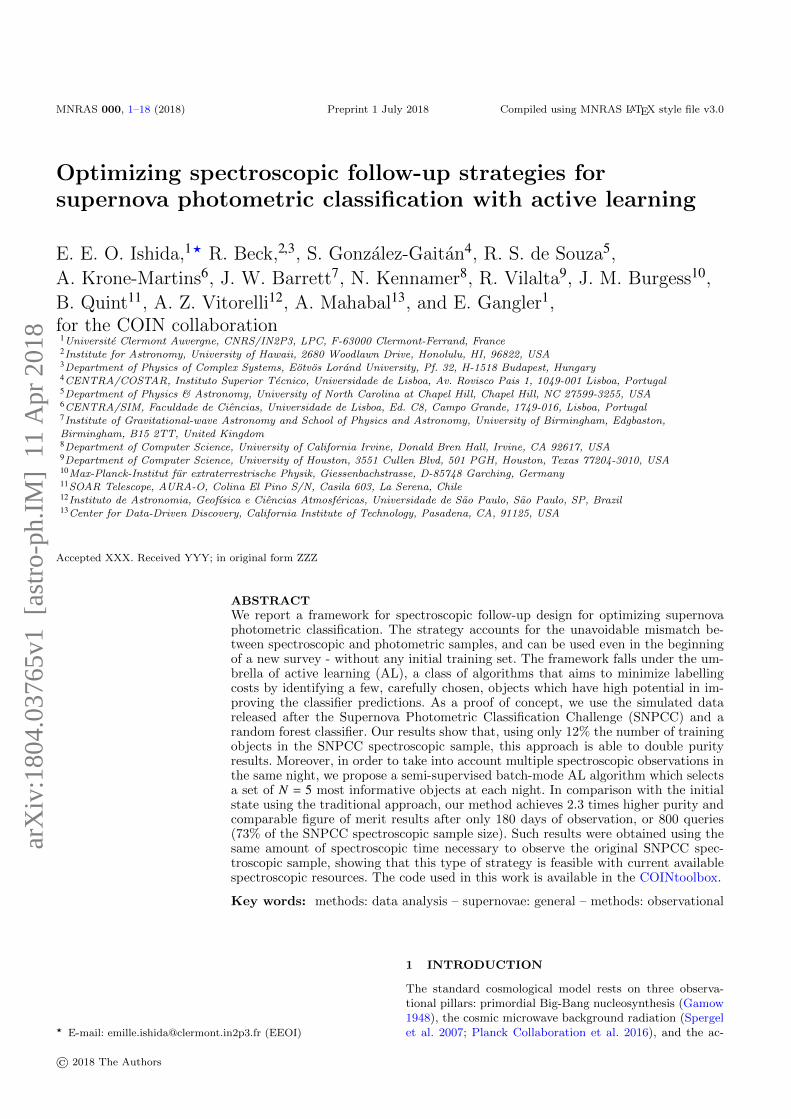
ABSTRACTWe report a framework for spectroscopic follow-up design for optimizing supernovaphotometric classification. The strategy accounts for the unavoidable mismatch be-tween spectroscopic and photometric samples, and can be used even in the beginningof a new survey - without any initial training set. The framework falls under the um-brella of active learning (AL), a class of algorithms that aims to minimize labellingcosts by identifying a few, carefully chosen, objects which have high potential in im-proving the classifier predictions. As a proof of concept, we use the simulated datareleased after the Supernova Photometric Classification Challenge (SNPCC) and arandom forest classifier. Our results show that, using only 12% the number of trainingobjects in the SNPCC spectroscopic sample, this approach is able to double purityresults. Moreover, in order to take into account multiple spectroscopic observations inthe same night, we propose a semi-supervised batch-mode AL algorithm which selectsa set of N = 5 most informative objects at each night. In comparison with the initialstate using the traditional approach, our method achieves 2.3 times higher purity andcomparable figure of merit results after only 180 days of observation, or 800 queries(73% of the SNPCC spectroscopic sample size). Such results were obtained using thesame amount of spectroscopic time necessary to observe the original SNPCC spec-troscopic sample, showing that this type of strategy is feasible with current availablespectroscopic resources. The code used in this work is available in the COINtoolbox.

Key words: methods: data analysis – supernovae: general – methods: observational

? E-mail: emille.ishida@clermont.in2p3.fr (EEOI)

1 INTRODUCTION

The standard cosmological model rests on three observa-tional pillars: primordial Big-Bang nucleosynthesis (Gamow1948), the cosmic microwave background radiation (Spergelet al. 2007; Planck Collaboration et al. 2016), and the ac-

© 2018 The Authors

arX

iv:1

804.

0376

5v1

[as

tro-

ph.I

M]

11

Apr

201

8

2 Ishida et al.

celerated cosmic expansion (Riess et al. 1998; Perlmutteret al. 1999) - with Type Ia supernovae (SNe Ia) playing animportant role in probing the last one. SNe Ia are astro-nomical transients which are used as standardizable candlesin the determination of extragalactic distances and veloci-ties (Hillebrandt & Niemeyer 2000; Goobar & Leibundgut2011). However, between the discovery of a SN candidateand its successful application in cosmological studies, addi-tional research steps are necessary.

Once a transient is identified as a potential SN, it mustgo through three main steps: i) classification, ii) redshift esti-mation, and iii) estimation of its standardized apparent mag-nitude at maximum brightness (Phillips 1993; Tripp 1998).Ideally, each SN thus requires at least one spectroscopic ob-servation (preferably around maximum - items i and ii) anda series of consecutive photometric measurements (item iii).Since we are not able to get spectroscopic measurement forall transient candidates, soon after a variable source is de-tected a decision must be made regarding its spectroscopicfollow-up, making coordination between transient imagingsurveys and spectroscopic facilities mandatory. From a tra-ditional perspective, taking a spectrum of a transient thatends up classified as a SNIa results in the object being in-cluded in the cosmological analysis. On the other hand, ifthe target is classified as non-Ia, spectroscopic time for cos-mology is essentially considered “lost”1.

In the last couple of decades, a strong community ef-fort has been devoted to the detection and follow-up of SNeIa for cosmology. Classifiers (human or artificial) on whichfollow-up decisions are based have become increasingly ef-ficient in identifying SNe Ia from early stages of their lightcurve evolution - successfully targeting them for spectro-scopic observations (e.g. Perrett et al. 2010). The availablecosmology data set has grown from 42 (Perlmutter et al.1999) to 740 (Betoule et al. 2014) in that period of time. Thissuccess helped building consensus around the paramount im-portance of SNe Ia for cosmology. It has also encouragedthe community to add even more objects to the Hubble dia-gram and to investigate the systematics uncertainties whichcurrently dominate dark energy error budget (e.g. Conleyet al. 2011). Thenceforth, SNe Ia are major targets of manycurrent - e.g. Dark Energy Survey2 (DES), Panoramic Sur-vey Telescope and Rapid Response System3 (Pan-STARRS)- and upcoming surveys - e.g. Zwicky Transient Facility4

(ZTF) and Large Synoptic Survey Telescope5 (LSST). Theselatter new surveys are expected to completely change thedata paradigm for SN cosmology, increasing the number ofavailable light curves by a few orders of magnitude.

However, to take full advantage of the great potentialin such large photometric data sets, we still have to con-tend with the fact that spectroscopic resources are - andwill continue to be - scarce. The majority of photometri-cally identified candidates will never be followed spectro-scopically. Full cosmological exploitation of wide-field imag-

1 This is strictly for cosmological purposes; spectroscopic obser-

vations are extremely valuable, irrespective of the transient inquestion, though for different scientific goals.2 https://www.darkenergysurvey.org/3 https://panstarrs.stsci.edu/4 http://www.ptf.caltech.edu/ztf/5 https://www.lsst.org/

ing surveys necessarily requires a framework able to infer re-liable spectroscopically-derived features (redshift and class)from purely photometric data. Provided a particular tran-sient has an identifiable host, redshift can be obtained be-fore/after the event from the host observations (spectro-scopic or photometric) or even from the light curve itself(e.g. Wang et al. 2015). On the other hand, classificationshould primarily be inferred from the light curve6. This pa-per concerns itself with the latter.

Before we dive into the details of SN photometric clas-sification, it is important to keep in mind that, regardless ofthe method chosen to circumvent these issues, photometricinformation will always carry a larger degree of uncertaintythan those from the spectroscopic scenario. Photometric red-shift estimations are expected to have non-negligible errorbars and, at the same time, any kind of classifier will carrysome contamination to the final SNIa sample. Neverthe-less, if we manage to keep these effects under control, weshould be able to use photometrically observed SNe Ia toincrease the statistical significance of our results. The ques-tion whether the final cosmological outcomes surpass thoseof the spectroscopic-only sample enough to justify the addi-tional effort is still debatable. Despite a few reports in thisdirection using real data from the Sloan Digital Sky Survey7

(SDSS - Hlozek et al. 2012; Campbell et al. 2013) and Pan-STARRS (Jones et al. 2017), the answer keeps changing asdifferent steps of the pipeline are improved and more databecome available. Nevertheless, there seems to be a consen-sus in the astronomical community that we have much togain from such an exercise.

The vast literature, with suggestions on how to im-prove/solve different stages of the SN photometric classi-fication pipeline, is a testimony of the positive attitudewith which the subject is approached. For more than 15years the field has been overwhelmed with attempts rely-ing on a wide range of methodologies: colour-colour andcolour-magnitude diagrams (Poznanski et al. 2002; Johnson& Crotts 2006), template fitting techniques (e.g. Sullivanet al. 2006), Bayesian probabilistic approaches (Poznanskiet al. 2007; Kuznetsova & Connolly 2007), fuzzy set theory(Rodney & Tonry 2009), kernel density methods (Newlinget al. 2011) and more recently, machine learning-based clas-sifiers (e.g. Richards et al. 2012a; Ishida & de Souza 2013;Karpenka et al. 2013; Lochner et al. 2016; Moller et al. 2016;Charnock & Moss 2017; Dai et al. 2017).

In 2010, the SuperNova Photometric ClassificationChallenge (SNPCC - Kessler et al. 2010) summarized thestate of the field by inviting different groups to apply theirclassifiers to the same simulated data set. Participants wereasked to classify a set of light curves generated accordingto the DES photometric sample characteristics. As a start-ing point, they were provided with a spectroscopic sampleenclosing ∼ 5% of the total data set, and for which classinformation was disclosed. The organizers posed three mainquestions: full light curve classification with and without theuse of redshift information (supposedly obtained from thehost galaxy) and an early epoch classification - where par-ticipants were allowed to use only the first 6 observed points

6 Although, see Foley & Mandel 2013.7 http://www.sdss.org/

MNRAS 000, 1–18 (2018)

Optimizing spectroscopic follow-up for SN photometric classification with AL 3

from each light curve. The goal of the latter was to access thecapability of different algorithms to advise on spectroscopictargeting while the SN was still bright enough to allow it.A total of 10 groups replied to the call, submitting 13 (9)entries for the full light curve classification with (without)the use of redshift information. No submission was receivedfor the early epoch scenario.

The algorithms competing in the SNPCC were quitediverse, including template fitting, statistical modelling, se-lection cuts and machine learning-based strategies (see sum-mary of all participants and result in Kessler et al. 2010).Classification results were consistent among different meth-ods with no particular algorithm clearly outperforming allthe others. The main legacy of this initiative however, wasthe updated public data set made available to the commu-nity once the challenge was completed. It became a testbench for experimentation, specially for machine learningapproaches (Newling et al. 2011; Richards et al. 2012a;Karpenka et al. 2013; Ishida & de Souza 2013).

One particularly challenging characteristic of the SNclassification problem, also present in the SNPCC data,is the discrepancy between spectroscopic and photometricsamples. In a supervised machine learning framework, wehave no alternative other than to use spectroscopically clas-sified SNe as training. This turns out to be a serious problem,since one of the hypothesis behind most text-book learn-ing algorithms relies on training being representative of tar-get. Due to the stringent observational requirements of spec-troscopy, this will never be the case between spectroscopicand photometric astronomical samples. But the situation iseven more drastic for SNe, where the spectroscopic follow-up strategy was designed to target as many Ia-like objectsas possible. Albeit modern low-redshift surveys try to miti-gate and counterbalance this effect (e.g. ASASSN8, iPTF9),the medium/high redshift (z > 0.1) spectroscopic sampleis still heavily under-represented by all non-Ia SNe types.Spectroscopic observations are so time demanding, and therate with which the photometric samples are increasing isso fast, that the situation is not expected to change evenwith dedicated spectrographs (OzDES - Childress et al.2017). This issue has been pointed out by many post-SNPCCmachine learning-based analysis (e.g. Richards et al. 2012a;Karpenka et al. 2013; Varughese et al. 2015; Lochner et al.2016; Charnock & Moss 2017; Revsbech et al. 2017). In spiteof the general consensus being that one should prioritizefaint objects for spectroscopic targeting, as an attempt toincrease representativeness (Richards et al. 2012a; Lochneret al. 2016), the details on how exactly this should be im-plemented are yet to be defined.

Thus the question still remains: how do we optimize thedistribution of spectroscopic resources with the goal of im-proving photometric SN identification? Or, in other words,how do we construct a training sample that maximizes ac-curate classification with a minimum number of labels, i.e.spectroscopically-classified SNe? The above question is sim-ilar in context to the ones addressed by an area of machinelearning called active learning (Settles 2012; Balcan et al.2009; Cohn et al. 1996).

8 http://www.astronomy.ohio-state.edu/assassin/index.shtml9 https://www.ptf.caltech.edu/iptf

Active Learning (AL) iteratively identifies which ob-jects in the target (photometric) sample would most likelyimprove the classifier if included in the training data - al-lowing sequential updates of the learning model with a min-imum number of labelled instances. It has been widely usedin a variety of different research fields, e.g. natural languageprocessing (Thompson et al. 1999), spam classification (De-Barr & Wechsler 2009), cancer detection (Liu 2004) andsentiment analysis (Kranjc et al. 2015). In astronomy, ALhas already been successfully applied in multiple tasks: de-termination of stellar population parameters (Solorio et al.2005), classification of variable stars (Richards et al. 2012b),optimization of telescope choice (Xia et al. 2016), static su-pernova photometric classification (Gupta et al. 2016), andphotometric redshift estimation (Vilalta et al. 2017). Thereare also reports based on similar ideas by Masters et al.(2015); Hoyle et al. (2016).

In this work, we show how active learning enables theconstruction of optimal training datasets for SNe photomet-ric classification, providing observers with a spectroscopicfollow-up protocol on a night-by-night basis. The frameworkrespects the time evolution of the survey providing a deci-sion process which can be implemented from the first obser-vational nights –avoiding the necessity of adapting legacydata and the consequent translation between different pho-tometric systems. The methodology herein employed virtu-ally allows any machine learning technique to outperformitself by simply labelling the data (taking the spectrum) ina way that provides maximum information gain to the clas-sifier. As a case study, we focus on the problem of binaryclassification, i.e. Type Ia vs non-Ia, but the overall struc-ture can be easily generalized for multi-classification tasks.

This paper is organized as follows: section 2 describesthe SNPCC data set, emphasizing the differences betweenspectroscopic and photometric samples. Section 3 details onthe feature extraction, classifier and metrics used through-out the paper. Section 4 explains the AL algorithm, detailsthe configurations we chose to approach the SN photometricclassification problem, and presents results for the idealizedstatic, full light curve scenario. Section 5 explains how ourapproach deals with the real-time evolution of the surveyand its consequent results. Section 6 presents our proposalfor real-time multiple same-night spectroscopic targeting(batch-mode AL). Having established a baseline data drivenspectroscopic strategy, in Section 7 we estimate the amountof telescope time necessary to observe the AL queried sam-ple. Lastly, section 8 shows our conclusions.

2 DATA

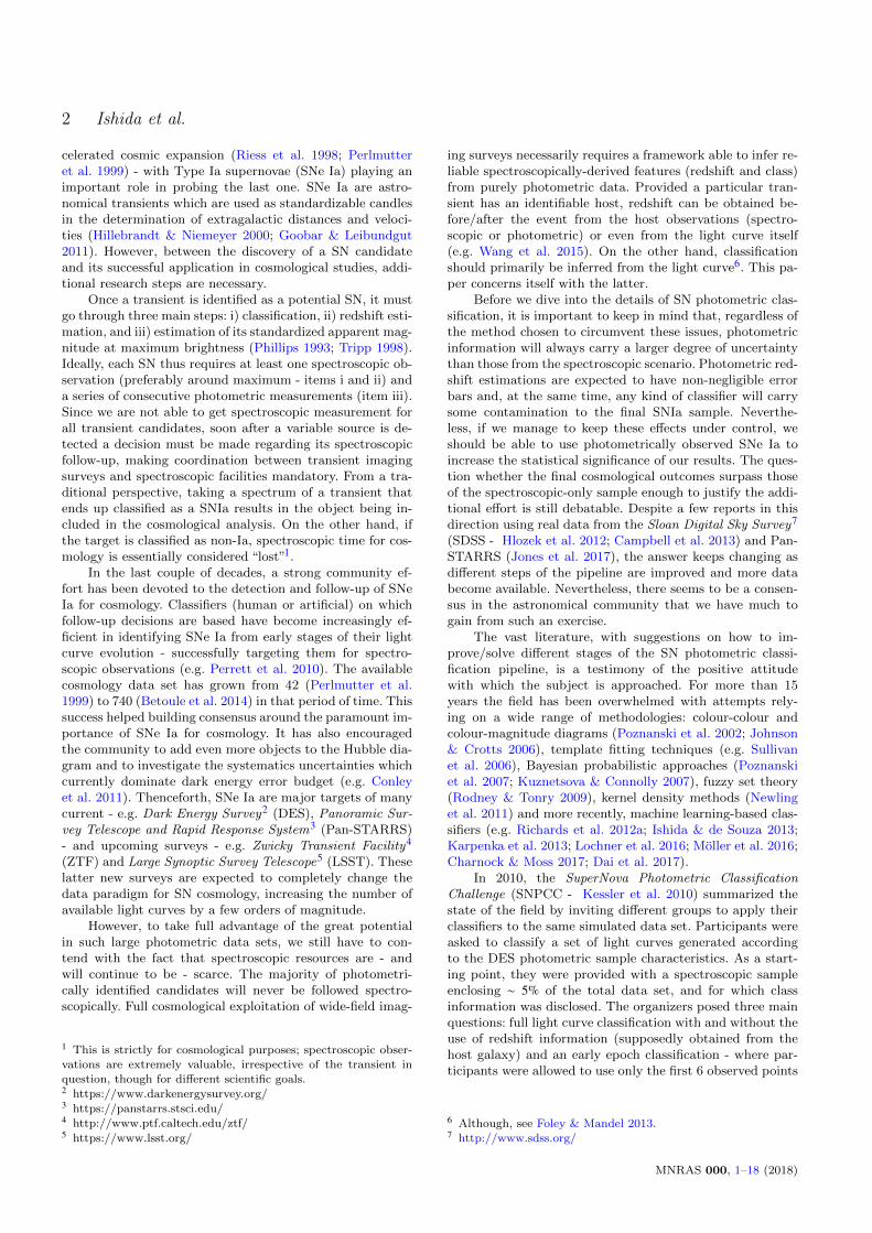
In what follows, we use the data released after the SNPCC.This is a simulated data set constructed to mimic DES ob-servations. The sample contains 20216 supernovae (SNe) ob-served in four DES filters, {g, r, i, z}, among which a subsetof 1103 are identified as belonging to the spectroscopic sam-ple. This subset was constructed considering observationsthrough a 4m (8m) telescope and limiting r-band magnitudeof 21 (23.5) (Kessler et al. 2010). Thus, it resembles closelybiases foreseen in a realistic spectroscopic sample when com-pared to the photometric one. Among them, we highlight thepredomination of brighter objects (figure 1) with higher sig-

MNRAS 000, 1–18 (2018)

4 Ishida et al.

Figure 1. Comparison between simulated peak magnitudes in

the SNPCC spectroscopic (red - training) and photometric (blue

- target) samples. Violin plots show both distributions in each ofthe DES filters.

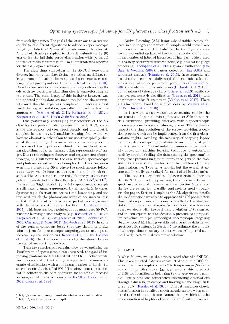
Figure 2. Distribution of mean signal to noise ratio (SNR) in

the SNPCC spectroscopic (red - training) and photometric (blue- target) samples.

nal to noise ratio (SNR, figure 2), and the predominance ofSNe Ia over other SN types (figure 3). Hereafter, the spec-troscopic sample will be designated SNPCC spec and theremaining objects will be addressed as SNPCC photo.

3 TRADITIONAL ANALYSIS

3.1 Feature extraction

For each supernova, we observe its light curve, i.e. the evo-lution of brightness (flux) as a function of time, in four DESfilters {g, r, i, z}. For most machine learning applications, thisinformation needs to be homogenized before it can be usedas input to a learning algorithm10. There are many waysin which this feature extraction step can be performed: viaa proposed analytical parametrization (Bazin et al. 2009;Newling et al. 2011), comparisons with theoretical and/orwell-observed templates (Sako et al. 2008) or dimensional-ity reduction techniques (Richards et al. 2012a; Ishida &de Souza 2013). The literature has many examples show-ing that, for the same classification algorithm, the choiceof the feature extraction method can significantly impact

10 Exceptions include algorithms able to deal with a high degree

of missing data (e.g. Charnock & Moss 2017; Naul et al. 2018).

Sample

SN ty

pe

Spec (train) Photo (target)

Ia

Ibc

II

SNPCC photoSNPCCspec

Ia

Ibc

II

Sample

SNetype

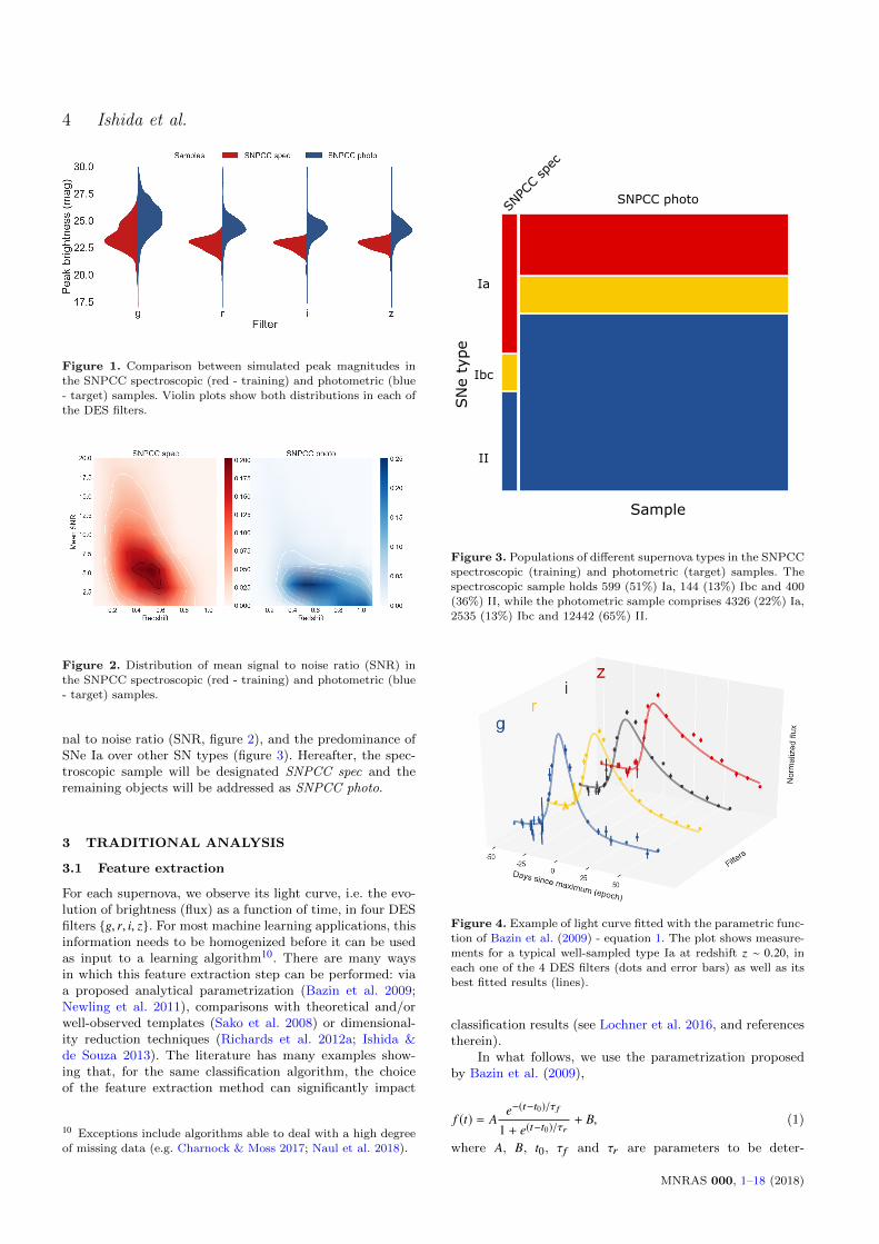
Figure 3. Populations of different supernova types in the SNPCC

spectroscopic (training) and photometric (target) samples. The

spectroscopic sample holds 599 (51%) Ia, 144 (13%) Ibc and 400(36%) II, while the photometric sample comprises 4326 (22%) Ia,

2535 (13%) Ibc and 12442 (65%) II.

Figure 4. Example of light curve fitted with the parametric func-tion of Bazin et al. (2009) - equation 1. The plot shows measure-ments for a typical well-sampled type Ia at redshift z ∼ 0.20, ineach one of the 4 DES filters (dots and error bars) as well as its

best fitted results (lines).

classification results (see Lochner et al. 2016, and referencestherein).

In what follows, we use the parametrization proposedby Bazin et al. (2009),

f (t) = Ae−(t−t0)/τ f

1 + e(t−t0)/τr+ B, (1)

where A, B, t0, τf and τr are parameters to be deter-

MNRAS 000, 1–18 (2018)

Optimizing spectroscopic follow-up for SN photometric classification with AL 5

Figure 5. Evolution of classification results as a function of the number of queries for the static full light curve analysis.

mined. We fit each filter independently in flux space witha Levenberg-Marquardt least-square minimization (Madsenet al. 2004). Figure 4 shows an example of flux measure-ments, corresponding errors and best-fit results in all 4 filtersfor a typical, well-sampled, SN Ia from SNPCC data.

3.2 Classifier

Once the data has been homogenized, we need a supervisedlearning model to harvest the information stored in the spec-troscopic sample. Analogous to the feature extraction case,the choice of classifier also impacts the final classificationresults for a given static data set (Lochner et al. 2016). Inorder to isolate the impact of AL in improving a given config-uration of feature extraction and machine learning pipeline,we chose to restrict our analysis to a single classifier. A com-plete study on how different classifiers respond to the updatein training provided by AL is out of the scope of this work,but is a crucial question to be answered in subsequent stud-ies. All the results we present below were obtained with arandom forest algorithm (Breiman 2001).

Random forest is a popular machine learning algorithmknown to achieve accurate results with minimal parametertuning. It is an ensemble technique made up of multiple de-cision trees (Breiman et al. 1984), constructed over different

sub-samples of the original data. Final results are obtainedby averaging over all trees (for further details, see appendicesA and B of Richards et al. 2012a). The method has been suc-cessfully used for SN photometric classification (Richardset al. 2012a; Lochner et al. 2016; Revsbech et al. 2017). Inwhat follows, we used the scikit-learn11 implementationof the algorithm with 1000 trees. In this context, the prob-ability of being a SN Ia, pIa, is given by the percentage oftrees in the ensemble voting for a SNIa classification12.

3.3 Metrics

The choice of a metric to quantify classification success goesbeyond the use of classical accuracy (equation 2) - especiallywhen the populations are unbalanced (figure 3). In order tooptimize information extraction, this choice must take intoaccount the scientific question at hand.

In the traditional SN case, the goal is to improve thequality of the final SNIa sample for further cosmological

11 http://scikit-learn.org/12 In this work we are concerned only with Ia × non-Ia classifi-cation. The analysis of classification performance using other SN

types will be the subject of a subsequent investigation.

MNRAS 000, 1–18 (2018)

6 Ishida et al.

Canonical Passive learning AL: Uncertainty sampling

18 21 24 27 18 21 24 27 18 21 24 27

900

700

500

250

100

50

40

30

20

10

i−band peak magnitude

Num

ber

of q

uerie

s

Training Target Queried objects

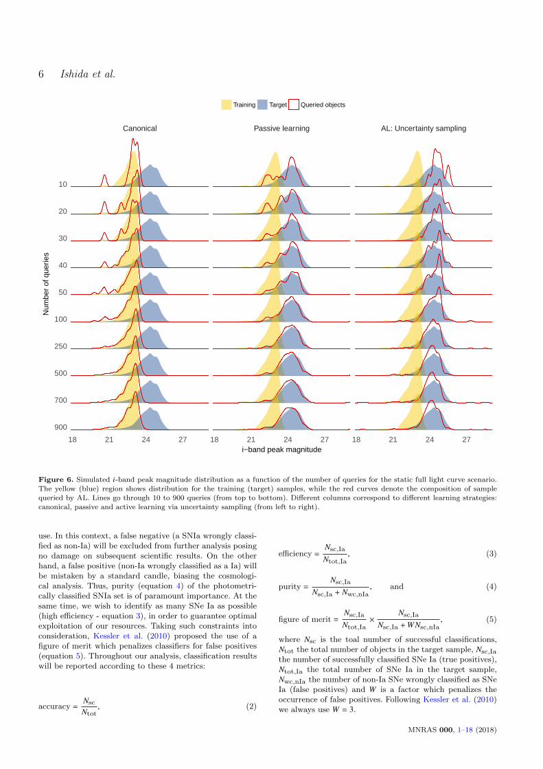
Figure 6. Simulated i-band peak magnitude distribution as a function of the number of queries for the static full light curve scenario.

The yellow (blue) region shows distribution for the training (target) samples, while the red curves denote the composition of samplequeried by AL. Lines go through 10 to 900 queries (from top to bottom). Different columns correspond to different learning strategies:

canonical, passive and active learning via uncertainty sampling (from left to right).

use. In this context, a false negative (a SNIa wrongly classi-fied as non-Ia) will be excluded from further analysis posingno damage on subsequent scientific results. On the otherhand, a false positive (non-Ia wrongly classified as a Ia) willbe mistaken by a standard candle, biasing the cosmologi-cal analysis. Thus, purity (equation 4) of the photometri-cally classified SNIa set is of paramount importance. At thesame time, we wish to identify as many SNe Ia as possible(high efficiency - equation 3), in order to guarantee optimalexploitation of our resources. Taking such constraints intoconsideration, Kessler et al. (2010) proposed the use of afigure of merit which penalizes classifiers for false positives(equation 5). Throughout our analysis, classification resultswill be reported according to these 4 metrics:

accuracy =Nsc

Ntot, (2)

efficiency =Nsc,Ia

Ntot,Ia, (3)

purity =Nsc,Ia

Nsc,Ia + Nwc,nIa, and (4)

figure of merit =Nsc,Ia

Ntot,Ia×

Nsc,Ia

Nsc,Ia +W Nsc,nIa, (5)

where Nsc is the toal number of successful classifications,Ntot the total number of objects in the target sample, Nsc,Ia

the number of successfully classified SNe Ia (true positives),Ntot,Ia the total number of SNe Ia in the target sample,Nwc,nIa the number of non-Ia SNe wrongly classified as SNeIa (false positives) and W is a factor which penalizes theoccurrence of false positives. Following Kessler et al. (2010)we always use W = 3.

MNRAS 000, 1–18 (2018)

Optimizing spectroscopic follow-up for SN photometric classification with AL 7

4 ACTIVE LEARNING

We now turn to the key missing ingredient in our pipeline.The tools we have described thus far allow us to process(section 3.1), classify (section 3.2), and evaluate classifica-tion results (section 3.3) given a pair of labelled and unla-belled light-curve data sets. The question now is: startingfrom this initial configuration, how can we optimize the useof subsequent spectroscopic resources in order to maximizethe potential of our classifier? Or in other words, how can weachieve high generalization performance by adding a mini-mum number of new spectroscopically observed objects tothe training sample? We advocate the use of a dedicated de-cision system tuned to choose the most informative objectsto be spectroscopically targeted.

Active learning (AL) is an area of machine learningdesigned to optimize learning results while minimizing thenumber of labelled instances. At each iteration, the algo-rithm suggests which of the unlabelled objects is most in-formative to the learning model (Settles 2012; Balcan et al.2009; Cohn et al. 1996). Once identified, this object is pro-vided a label (i.e. queried) and added to the original train-ing sample to re-train the model (figure 7); the process isrepeated until convergence is achieved, or until labelling re-sources are exhausted.

Different flavours of AL propose different strategies toidentify which objects should be queried. In what follows,we report results obtained using pool-based AL13 via un-certainty sampling, where, at each iteration, we choose toquery the object with the largest uncertainty in the pre-dicted class14. A detailed explanation of the uncertaintysampling technique (as well as query by committee) is givenin appendix A.

Finally, whenever one wishes to quantify the improve-ment in classification results due to AL, it is important tokeep in mind that simply increasing the number of objectsavailable for training changes the state of the model - in-dependently of how the extra data were chosen. Thus, ALresults should always be compared to the passive learningstrategy, where at each iteration objects to be queried arerandomly drawn from the unlabelled sample. Moreover, inthe specific case of SN classification, we also want to in-vestigate how the learning model would behave if the samenumber of objects were queried following the canonical spec-troscopic targeting strategy - where objects to be queriedare randomly drawn from a sample which follows closelythe initial SNPCC labelled distribution. Diagnostic resultspresented bellow show outcomes from all three strategies:canonical, passive learning, and AL via uncertainty sam-pling15.

13 Our analysis used the libact Python package developed byYang et al. (2017).14 Given that we are using a random forest algorithm under bi-nary, Ia × non-Ia, classification, the object with highest uncer-

tainty will be the one with pIa closest to 0.5.15 The code used in this paper can be found in the COINtoolbox

- https://github.com/COINtoolbox/ActSNClass

Figure 7. Schematic illustration of the Active Learning (AL)

work flow in the context of photometric light curves classification.Starting at the top left, the training set (spectroscopic sample -

grey circles), is used to train a machine learning algorithm - re-sulting in a model which is then applied to the unlabelled data

(photometric light-curves - yellow pentagons). This initial model

returns a classification for each data point of the unlabelled set(now represented as red squares and blue triangles). The AL al-

gorithm is then used to choose a data point of the unlabelled data

with highest potential to improve the classification model (iden-tified by the grey arrow). The label of this point is then queried

(a spectrum is taken). Once the true label of the queried point

is known, it is added to the training set (converted into a greycircle), and the process is repeated.

4.1 Static full light curve analysis

We begin by applying the complete framework describedin the previous subsections to static data. This is the tradi-tional approach, where we consider that all light curves werecompletely observed at the start of the analysis. Althoughthis is not a realistic scenario (one cannot query, or spec-troscopically observe, a SN that has already faded away), itgives us an upper limit on estimated classification results.Section 5 considers more realistic constraints on availablequery data and light-curve evolution.

For each light curve and filter, all available data pointswere used to find the best-fit parameters of equation 1 fol-lowing the procedure described in section 3. Best-fit valuesfor different filters were concatenated to compose a line inthe data matrix. In order to ensure the quality of fit, weconsidered only SNe with a minimum of 5 observed epochsin each filter; this reduced the size of our spectroscopic andphotometric samples to 1094 and 20193 objects, respectively.

MNRAS 000, 1–18 (2018)

8 Ishida et al.

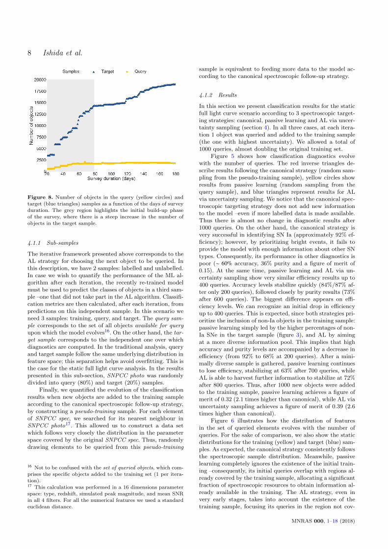
Figure 8. Number of objects in the query (yellow circles) andtarget (blue triangles) samples as a function of the days of survey

duration. The grey region highlights the initial build-up phase

of the survey, where there is a steep increase in the number ofobjects in the target sample.

4.1.1 Sub-samples

The iterative framework presented above corresponds to theAL strategy for choosing the next object to be queried. Inthis description, we have 2 samples: labelled and unlabelled.In case we wish to quantify the performance of the ML al-gorithm after each iteration, the recently re-trained modelmust be used to predict the classes of objects in a third sam-ple –one that did not take part in the AL algorithm. Classifi-cation metrics are then calculated, after each iteration, frompredictions on this independent sample. In this scenario weneed 3 samples: training, query, and target. The query sam-ple corresponds to the set of all objects available for queryupon which the model evolves16. On the other hand, the tar-get sample corresponds to the independent one over whichdiagnostics are computed. In the traditional analysis, queryand target sample follow the same underlying distribution infeature space; this separation helps avoid overfitting. This isthe case for the static full light curve analysis. In the resultspresented in this sub-section, SNPCC photo was randomlydivided into query (80%) and target (20%) samples.

Finally, we quantified the evolution of the classificationresults when new objects are added to the training sampleaccording to the canonical spectroscopic follow-up strategy,by constructing a pseudo-training sample. For each elementof SNPCC spec, we searched for its nearest neighbour inSNPCC photo17. This allowed us to construct a data setwhich follows very closely the distribution in the parameterspace covered by the original SNPCC spec. Thus, randomlydrawing elements to be queried from this pseudo-training

16 Not to be confused with the set of queried objects, which com-prises the specific objects added to the training set (1 per itera-

tion).17 This calculation was performed in a 16 dimensions parameter

space: type, redshift, simulated peak magnitude, and mean SNRin all 4 filters. For all the numerical features we used a standard

euclidean distance.

sample is equivalent to feeding more data to the model ac-cording to the canonical spectroscopic follow-up strategy.

4.1.2 Results

In this section we present classification results for the staticfull light curve scenario according to 3 spectroscopic target-ing strategies: canonical, passive learning and AL via uncer-tainty sampling (section 4). In all three cases, at each itera-tion 1 object was queried and added to the training sample(the one with highest uncertainty). We allowed a total of1000 queries, almost doubling the original training set.

Figure 5 shows how classification diagnostics evolvewith the number of queries. The red inverse triangles de-scribe results following the canonical strategy (random sam-pling from the pseudo-training sample), yellow circles showresults from passive learning (random sampling from thequery sample), and blue triangles represent results for ALvia uncertainty sampling. We notice that the canonical spec-troscopic targeting strategy does not add new informationto the model –even if more labelled data is made available.Thus there is almost no change in diagnostic results after1000 queries. On the other hand, the canonical strategy isvery successful in identifying SN Ia (approximately 92% ef-ficiency); however, by prioritizing bright events, it fails toprovide the model with enough information about other SNtypes. Consequently, its performance in other diagnostics ispoor (∼ 60% accuracy, 36% purity and a figure of merit of0.15). At the same time, passive learning and AL via un-certainty sampling show very similar efficiency results up to400 queries. Accuracy levels stabilize quickly (84%/87% af-ter only 200 queries), followed closely by purity results (73%after 600 queries). The biggest difference appears on effi-ciency levels. We can recognize an initial drop in efficiencyup to 400 queries. This is expected, since both strategies pri-oritize the inclusion of non-Ia objects in the training sample:passive learning simply led by the higher percentages of non-Ia SNe in the target sample (figure 3), and AL by aimingat a more diverse information pool. This implies that highaccuracy and purity levels are accompanied by a decrease inefficiency (from 92% to 68% at 200 queries). After a mini-mally diverse sample is gathered, passive learning continuesto lose efficiency, stabilizing at 63% after 700 queries, whileAL is able to harvest further information to stabilize at 72%after 800 queries. Thus, after 1000 new objects were addedto the training sample, passive learning achieves a figure ofmerit of 0.32 (2.1 times higher than canonical), while AL viauncertainty sampling achieves a figure of merit of 0.39 (2.6times higher than canonical).

Figure 6 illustrates how the distribution of featuresin the set of queried elements evolves with the number ofqueries. For the sake of comparison, we also show the staticdistributions for the training (yellow) and target (blue) sam-ples. As expected, the canonical strategy consistently followsthe spectroscopic sample distribution. Meanwhile, passivelearning completely ignores the existence of the initial train-ing –consequently, its initial queries overlap with regions al-ready covered by the training sample, allocating a significantfraction of spectroscopic resources to obtain information al-ready available in the training. The AL strategy, even invery early stages, takes into account the existence of thetraining sample, focusing its queries in the region not cov-

MNRAS 000, 1–18 (2018)

Optimizing spectroscopic follow-up for SN photometric classification with AL 9

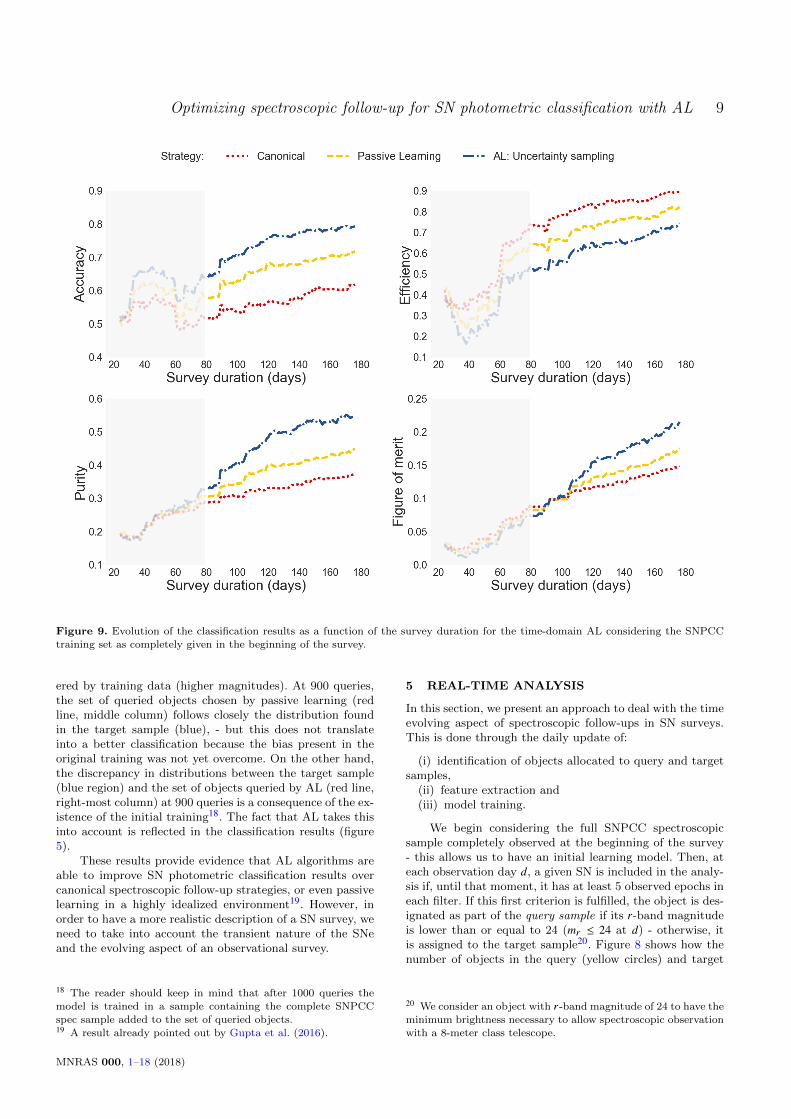
Figure 9. Evolution of the classification results as a function of the survey duration for the time-domain AL considering the SNPCC

training set as completely given in the beginning of the survey.

ered by training data (higher magnitudes). At 900 queries,the set of queried objects chosen by passive learning (redline, middle column) follows closely the distribution foundin the target sample (blue), - but this does not translateinto a better classification because the bias present in theoriginal training was not yet overcome. On the other hand,the discrepancy in distributions between the target sample(blue region) and the set of objects queried by AL (red line,right-most column) at 900 queries is a consequence of the ex-istence of the initial training18. The fact that AL takes thisinto account is reflected in the classification results (figure5).

These results provide evidence that AL algorithms areable to improve SN photometric classification results overcanonical spectroscopic follow-up strategies, or even passivelearning in a highly idealized environment19. However, inorder to have a more realistic description of a SN survey, weneed to take into account the transient nature of the SNeand the evolving aspect of an observational survey.

18 The reader should keep in mind that after 1000 queries the

model is trained in a sample containing the complete SNPCCspec sample added to the set of queried objects.19 A result already pointed out by Gupta et al. (2016).

5 REAL-TIME ANALYSIS

In this section, we present an approach to deal with the timeevolving aspect of spectroscopic follow-ups in SN surveys.This is done through the daily update of:

(i) identification of objects allocated to query and targetsamples,

(ii) feature extraction and(iii) model training.

We begin considering the full SNPCC spectroscopicsample completely observed at the beginning of the survey- this allows us to have an initial learning model. Then, ateach observation day d, a given SN is included in the analy-sis if, until that moment, it has at least 5 observed epochs ineach filter. If this first criterion is fulfilled, the object is des-ignated as part of the query sample if its r-band magnitudeis lower than or equal to 24 (mr ≤ 24 at d) - otherwise, itis assigned to the target sample20. Figure 8 shows how thenumber of objects in the query (yellow circles) and target

20 We consider an object with r-band magnitude of 24 to have theminimum brightness necessary to allow spectroscopic observation

with a 8-meter class telescope.

MNRAS 000, 1–18 (2018)

10 Ishida et al.

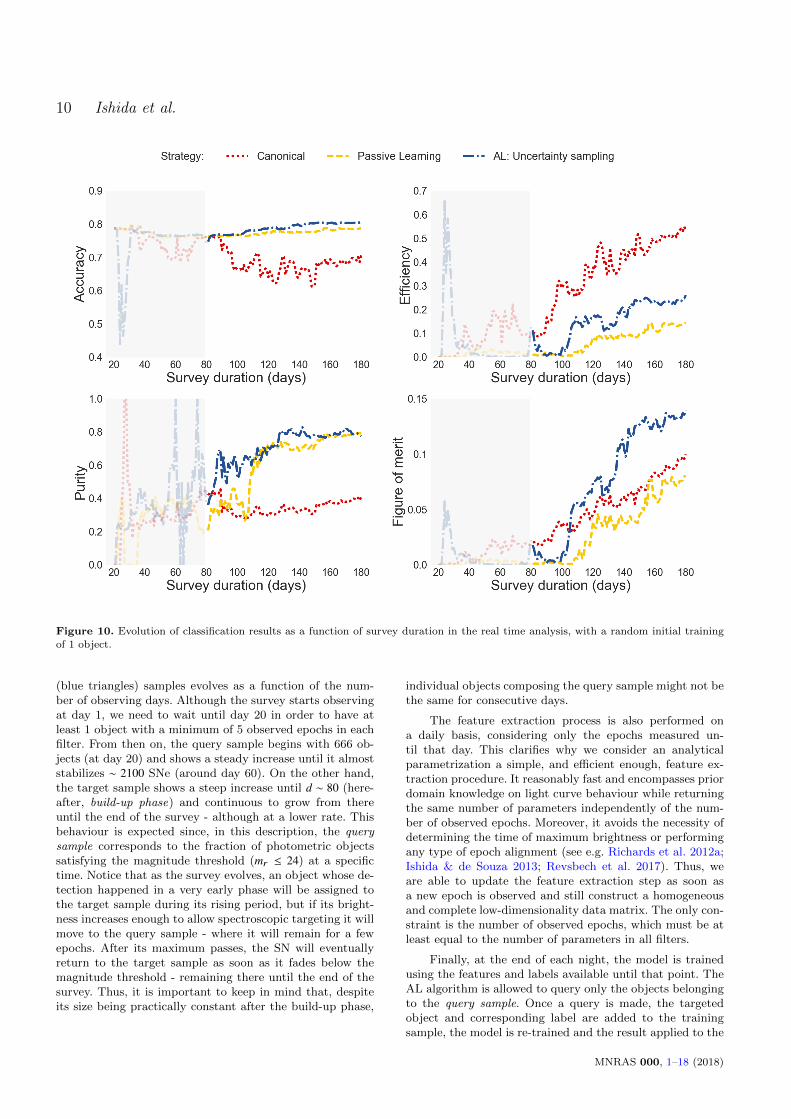
Figure 10. Evolution of classification results as a function of survey duration in the real time analysis, with a random initial training

of 1 object.

(blue triangles) samples evolves as a function of the num-ber of observing days. Although the survey starts observingat day 1, we need to wait until day 20 in order to have atleast 1 object with a minimum of 5 observed epochs in eachfilter. From then on, the query sample begins with 666 ob-jects (at day 20) and shows a steady increase until it almoststabilizes ∼ 2100 SNe (around day 60). On the other hand,the target sample shows a steep increase until d ∼ 80 (here-after, build-up phase) and continuous to grow from thereuntil the end of the survey - although at a lower rate. Thisbehaviour is expected since, in this description, the querysample corresponds to the fraction of photometric objectssatisfying the magnitude threshold (mr ≤ 24) at a specifictime. Notice that as the survey evolves, an object whose de-tection happened in a very early phase will be assigned tothe target sample during its rising period, but if its bright-ness increases enough to allow spectroscopic targeting it willmove to the query sample - where it will remain for a fewepochs. After its maximum passes, the SN will eventuallyreturn to the target sample as soon as it fades below themagnitude threshold - remaining there until the end of thesurvey. Thus, it is important to keep in mind that, despiteits size being practically constant after the build-up phase,

individual objects composing the query sample might not bethe same for consecutive days.

The feature extraction process is also performed ona daily basis, considering only the epochs measured un-til that day. This clarifies why we consider an analyticalparametrization a simple, and efficient enough, feature ex-traction procedure. It reasonably fast and encompasses priordomain knowledge on light curve behaviour while returningthe same number of parameters independently of the num-ber of observed epochs. Moreover, it avoids the necessity ofdetermining the time of maximum brightness or performingany type of epoch alignment (see e.g. Richards et al. 2012a;Ishida & de Souza 2013; Revsbech et al. 2017). Thus, weare able to update the feature extraction step as soon asa new epoch is observed and still construct a homogeneousand complete low-dimensionality data matrix. The only con-straint is the number of observed epochs, which must be atleast equal to the number of parameters in all filters.

Finally, at the end of each night, the model is trainedusing the features and labels available until that point. TheAL algorithm is allowed to query only the objects belongingto the query sample. Once a query is made, the targetedobject and corresponding label are added to the trainingsample, the model is re-trained and the result applied to the

MNRAS 000, 1–18 (2018)

Optimizing spectroscopic follow-up for SN photometric classification with AL 11

target sample (figure 7). Given the time span of the SNPCCdata, we are able to repeat this analysis for a total of 180days.

Figure 9 shows the evolution of classification resultsconsidering the complete SNPCC spectroscopic sample asa starting point. Here we can clearly see the effect of theevolving sample sizes: accuracy and efficiency results oscil-late, while purity and figure of merit remain indifferent tothe learning strategy, during the build-up phase (grey re-gion). Once this phase is over, results start to differ and theAL with uncertainty sampling clearly surpasses the othertwo, achieving 80% accuracy, 55% purity and a figure ofmerit of 0.23, while the passive learning only goes up to72% accuracy, 45% purity and figure of merit of 0.18. Thecanonical strategy continues to output better efficiency, butits loss in purity does not allow it to overcome even passivelearning in figure of merit levels.

5.1 No initial training

This leaves one open question: what should we do at thebeginning of a given survey, when a training set with thesame instrument characteristics (e.g. photometric system) isnot yet available? Or even more drastically: if the algorithmis capable of building its own training sample, do we evenneed an initial training at all? The answer is no.

Figure 10 shows how the classification results behavewhen the initial model is trained in 1 randomly selected ob-ject from the query sample, meaning we start with a randomclassifier. In this context, diagnostics are meaningless untilaround 100 days (a little after the build-up phase) when allsamples involved are under construction. After this period,AL with uncertainty sampling starts to dominate purity and,consequently, figure of merit results. After 150 observationdays (or after 130 objects were added to the training), theactive and passive learning strategies achieve purity levelscomparable to the one obtained in the unrealistic full lightcurve scenario (∼ 80%). Thus, at the end of the survey, ALefficiency results (27%) are 80% higher than the one ob-tained by passive learning (15%), which translates into analmost doubled figure of merit (0.14 from AL and 0.08 fromthe canonical strategy). Compare these results with the ini-tial state of the full light curve analysis: figure 5 (accuracy60%, efficiency 92%, purity of 35% and 0.15 figure of merit)was obtained using complete light curves for all objects, allSNe in the original SNPCC spectroscopic sample survivingthe minimum number of epochs cuts (1094 objects) and thesame random forest classifier. Final results of the real-timeAL analysis (figure 10) surpasses the full light curve initialstate accuracy results in 33%, more than doubles purity andachieves comparable figure of merit results. All of these whilerespecting the time evolution of observed epochs of only 161SNe in the training set, or 15% the number of objects in theoriginal SNPCC spectroscopic sample.

Accuracy levels of real time AL with (figure 9) and with-out (figure 10) the full initial training sample are compara-ble, while efficiency and figure of merit are higher for theformer case. However, purity levels are 45% higher withoutusing the initial training. This is a natural consequence ofthe higher number of SNe Ia in the SNPCC spectroscopicsample (figure 8), which requires the algorithm to unlearnthe preference for Ia classifications before it can achieve its

full potential in purity results. Figure 10 also shows that re-garding purity, passive learning is able to achieve the sameresults as those obtained with uncertainty sampling whileefficiency is severely compromised –exactly the opposite be-haviour shown by the canonical strategy. This is a conse-quence of the populations targeted by each of these strate-gies. By prioritizing brighter objects, the canonical strategyintroduces a bias in the learning model towards SNIa clas-sifications. On the other hand, by randomly sampling fromthe target, passive learning adds a larger number of non-Iaexamples to the training, introducing an opposite bias, atleast in the early stages of the survey.

In summary, given the intrinsic bias present in all canon-ically obtained samples, we advocate that the best strategyfor a new survey is to construct its own training during thefirsts running seasons. Letting its own photometric sampleguide the decisions of spectroscopic targeting. This is spe-cially important if one has the final goal of supernova cos-mology in mind, where the main objective is to maximizepurity (minimize false positives) as well as many other sci-entific SN objectives.

6 BATCH-MODE ACTIVE LEARNING

In this section, we take another step towards a more realisticdescription of a spectroscopic follow-up scenario. Instead ofchoosing one SN at a time, spectroscopic follow-up resourcesfor large scale surveys will probably allow a number of SNeto be spectroscopically observed per night. Thus, we need astrategy which allows us to extend the AL algorithm, opti-mizing our choice from one to a set (or a batch) of objects ateach iteration. We focus on two methods derived from thenotion of uncertainty sampling: N-least certain and Semi-supervised uncertainty sampling.

The N-least certain batch query strategy uses the samemachinery described in the sequential uncertainty samplingmethod but, instead of choosing a single unlabelled exam-ple, it selects the N objects with highest uncertainties, andqueries all of them. This tactic carries a disadvantage, since aset of objects whose predictions exhibit similar uncertaintieswill probably also be similar among themselves (i.e., will beclose to each other in the feature space). Thus, querying fora set of labels is not likely to lead to a model much differentthan the one obtained by adding only the most uncertainobject to the training set. In dealing with a batch mode sce-nario, we should also require that the elements of the batchbe as diverse as possible (maximizing their distance in thefeature space).

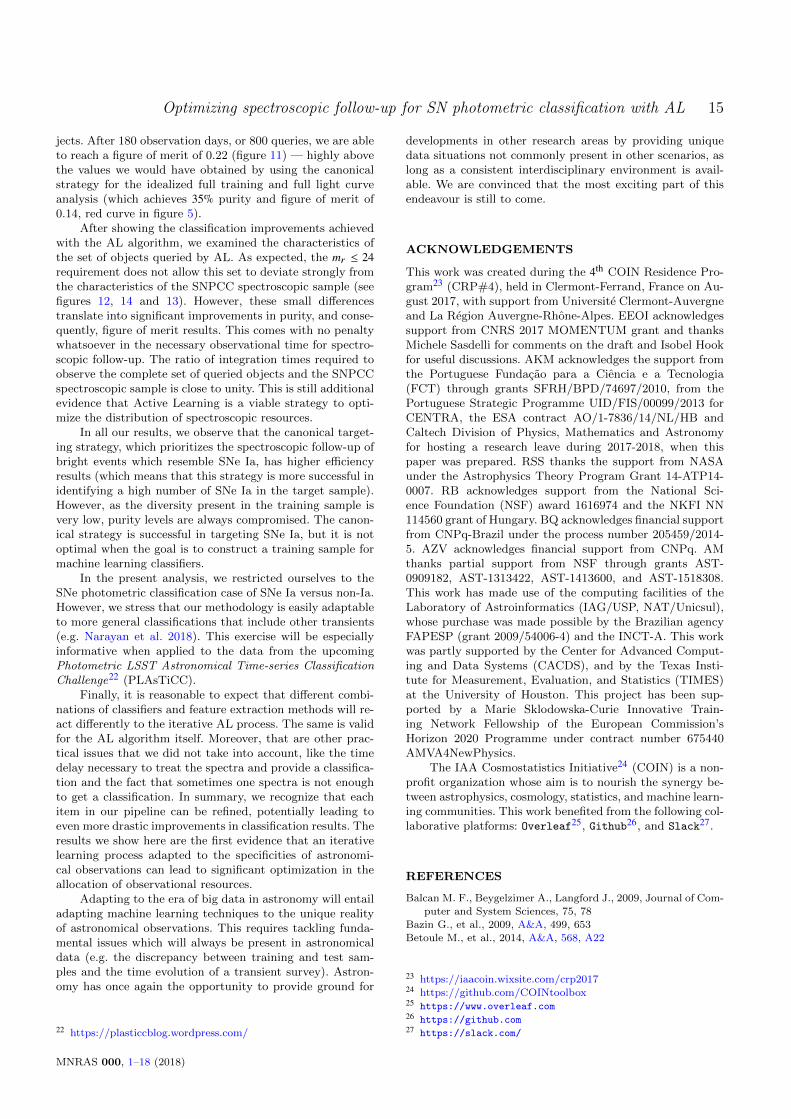
Semi-supervised uncertainty sampling (e.g. Hoi et al.2008), in contrast, avoids the need to call the oracle at eachindividual iteration by using the uncertainty associated toeach predicted label as a proxy for class assignment. Thealgorithm must be trained in the available initial sample inorder to create the first batch. The object with the great-est classification uncertainty is then identified. Suppose thisobject has a probability p of being SN Ia. A pseudo-label isthen drawn from a Bernoulli distribution, where success isinterpreted as “Ia” label (with probability p) and failure as“non-Ia”(with probability 1−p). The object features and cor-responding pseudo-label are temporarily added to the train-ing sample and the model is re-trained. This is repeated until

MNRAS 000, 1–18 (2018)

12 Ishida et al.

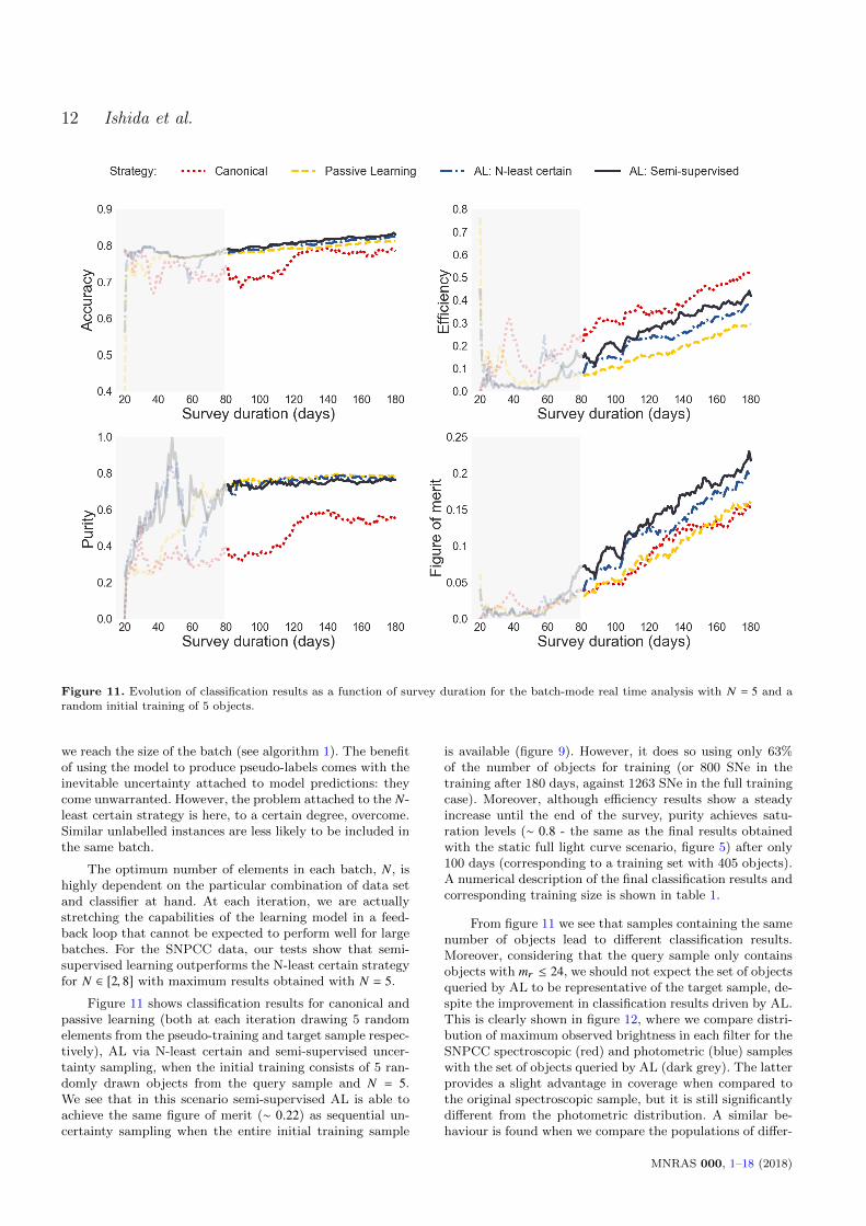
Figure 11. Evolution of classification results as a function of survey duration for the batch-mode real time analysis with N = 5 and a

random initial training of 5 objects.

we reach the size of the batch (see algorithm 1). The benefitof using the model to produce pseudo-labels comes with theinevitable uncertainty attached to model predictions: theycome unwarranted. However, the problem attached to the N-least certain strategy is here, to a certain degree, overcome.Similar unlabelled instances are less likely to be included inthe same batch.

The optimum number of elements in each batch, N, ishighly dependent on the particular combination of data setand classifier at hand. At each iteration, we are actuallystretching the capabilities of the learning model in a feed-back loop that cannot be expected to perform well for largebatches. For the SNPCC data, our tests show that semi-supervised learning outperforms the N-least certain strategyfor N ∈ [2, 8] with maximum results obtained with N = 5.

Figure 11 shows classification results for canonical andpassive learning (both at each iteration drawing 5 randomelements from the pseudo-training and target sample respec-tively), AL via N-least certain and semi-supervised uncer-tainty sampling, when the initial training consists of 5 ran-domly drawn objects from the query sample and N = 5.We see that in this scenario semi-supervised AL is able toachieve the same figure of merit (∼ 0.22) as sequential un-certainty sampling when the entire initial training sample

is available (figure 9). However, it does so using only 63%of the number of objects for training (or 800 SNe in thetraining after 180 days, against 1263 SNe in the full trainingcase). Moreover, although efficiency results show a steadyincrease until the end of the survey, purity achieves satu-ration levels (∼ 0.8 - the same as the final results obtainedwith the static full light curve scenario, figure 5) after only100 days (corresponding to a training set with 405 objects).A numerical description of the final classification results andcorresponding training size is shown in table 1.

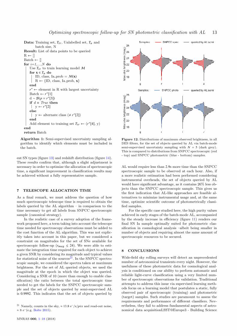
From figure 11 we see that samples containing the samenumber of objects lead to different classification results.Moreover, considering that the query sample only containsobjects with mr ≤ 24, we should not expect the set of objectsqueried by AL to be representative of the target sample, de-spite the improvement in classification results driven by AL.This is clearly shown in figure 12, where we compare distri-bution of maximum observed brightness in each filter for theSNPCC spectroscopic (red) and photometric (blue) sampleswith the set of objects queried by AL (dark grey). The latterprovides a slight advantage in coverage when compared tothe original spectroscopic sample, but it is still significantlydifferent from the photometric distribution. A similar be-haviour is found when we compare the populations of differ-

MNRAS 000, 1–18 (2018)

Optimizing spectroscopic follow-up for SN photometric classification with AL 13

Data: Training set, Ttr , Unlabelled set, Tu andbatch size, N

Result: List of data points to be queriedR ← []Batch ← []for i=1,...,N do

Use Ttr to train learning model Mfor x ∈ Tu do

ID, class, Ia prob = M(x)R ← {ID, class, Ia prob, x}

endr∗ ← element in R with largest uncertaintyBatch ← r∗[1]d ∼ B(p = r∗[3])if d ≡ True then

y ← r∗[2]else

y ← alternate class (, r∗[2])endAdd element to training set Ttr ← (r∗[4], y)

endreturn Batch

Algorithm 1: Semi-supervised uncertainty sampling al-gorithm to identify which elements must be included inthe batch.

ent SN types (figure 13) and redshift distribution (figure 14).These results confirm that, although a slight adjustment isnecessary in order to optimize the allocation of spectroscopictime, a significant improvement in classification results maybe achieved without a fully representative sample.

7 TELESCOPE ALLOCATION TIME

As a final remark, we must address the question of howmuch spectroscopic telescope time is required to obtain thelabels queried by the AL algorithm – in comparison to thetime necessary to get all labels from SNPCC spectroscopicsample (canonical strategy).

In the realistic case of a survey adoption of the frame-work proposed here, a term taking into account the telescopetime needed for spectroscopy observations must be added tothe cost function of the AL algorithm. This was not explic-itly taken into account in this paper, but we considered aconstraint on magnitudes for the set of SNe available forspectroscopic follow-up (rmag ≤ 24). We were able to esti-mate the integration time required for each object to achievea given SNR by considering its magnitude and typical valuesfor statistical noise of the sources21. In the SNPCC spectro-scopic sample, we considered the spectra taken at maximumbrightness. For the set of AL queried objects, we used themagnitude at the epoch in which the object was queried.Considering a SNR of 10 (more than enough to enable clas-sification) the ratio between the total spectroscopic timeneeded to get the labels for the SNPCC spectroscopic sam-ple and the set of objects queried by semi-supervised ALis 0.9992. This indicates that the set of objects queried by

21 Namely, counts in the sky, ≈ 13.8 e−/s/pix and read-out noise,

≈ 8 e−(e.g. Bolte 2015).

Figure 12. Distributions of maximum observed brightness, in allDES filters, for the set of objects queried by AL via batch-mode

semi-supervised uncertainty sampling with N = 5 (dark grey).

This is compared to distributions from SNPCC spectroscopic (red- top) and SNPCC photometric (blue - bottom) samples.

AL would require less than 2.9s more time than the SNPCCspectroscopic sample to be observed at each hour. Also, ifa more realistic estimation had been performed consideringinstrumental overheads, the set of objects queried by ALwould have significant advantage, as it contains 26% less ob-jects than the SNPCC spectroscopic sample. This gives usthe first indication that AL-like approaches are feasible al-ternatives to minimize instrumental usage and, at the sametime, optimize scientific outcome of photometrically classi-fied samples.

For the specific case studied here, the high purity valuesachieved in early stages of the batch-mode AL, accompaniedby the steady increase in efficiency (figure 11) renders ourfinal SN Ia sample optimally suited for photometric clas-sification in cosmological analysis –albeit being smaller innumber of objects and requiring almost the same amount ofspectroscopic resources to be secured.

8 CONCLUSIONS

Wide-field sky rolling surveys will detect an unprecedentednumber of astronomical transients every night. However, theusefulness of these photometric data for cosmological anal-ysis is conditioned on our ability to perform automatic andreliable light-curve classification using a very limited num-ber of spectroscopic observations for validation. Traditionalattempts to address this issue via supervised learning meth-ods focus on a learning model that postulates a static, fullyobserved pair of spectroscopic (training) and photometric(target) samples. Such studies are paramount to assess therequirements and performance of different classifiers. Nev-ertheless, they fail to address fundamental aspects of astro-nomical data acquisitionLSST@Europe3 - Building Science

MNRAS 000, 1–18 (2018)

14 Ishida et al.

static, full LC time domain time domaintime domain

initial training initial training initial training

UNC UNC BATCH 5 BATCH 5

training2093 1255 1093 810

size

accuracy 0.89 0.80 0.85 0.83

efficiency 0.73 0.78 0.69 0.44purity 0.78 0.55 0.69 0.76

figure of merit 0.39 0.23 0.31 0.22

Table 1. Classification results for the AL by uncertainty sampling (UNC) and semi-supervised batch mode (BATCH 5) strategies.

Sample

SN ty

pe

SNPCC train AL

query SNPCC photo

Ia

Ibc

II

SNPCC photoAL: semi

SNPCCspec

Ia

Ibc

II

Sample

SNetype

Figure 13. Populations of different supernova types in the orig-inal SNPCC spectroscopic and photometric samples, and in time

domain batch mode (N = 5) semi-supervised AL query sample

after 180 days of observations. The composition of the SNPCCsamples are the same as shown in figure 3. The AL query sample

holds 390 (48%) Ia, 122 (15%) Ibc and 298 (37%) II.

Collaborations (11-15 juin 201, which renders the problemill-suited for text-book machine learning algorithms. Themost crucial of these issues is the distributional discrepancybetween spectroscopic and photometric samples.

This mismatch has its origins in a follow-up strategydesigned to maximize the number of spectroscopically con-firmed SNe Ia for cosmology, resulting in a highly biasedspectroscopic set — and a sub-optimal training sample.Given such data configuration, not even the most suitableclassifier can be expected to achieve its full potential. In thiswork, we advocate that any attempt to improve SN pho-tometric classification must include a detailed strategy forconstructing a more representative training set, without ig-noring the constraints intrinsic to the observational process.

Our proposed framework updates on a daily basis cru-cial steps of the SN photometric classification pipeline anduses active learning to optimize the scientific outcome frommachine learning algorithms. On each day, we consider only

Figure 14. Redshift distribution of the original SNPCC spectro-

scopic (red - dotted) and photometric (blue - dashed) samples,

superimposed to the redshift distribution of the AL query set forthe time domain semi-supervised batch mode AL strategy with-

out the use of an initial training (dark blue - full). In each obser-

vation night, the algorithm queried for 5 SNe. The distributionshows redshift for the query sample after 180 observation nights.

.

the set of available observed epochs, and perform featureextraction via a parametric light-curve representation. Theidentification of SNe available for spectroscopic targeting(objects with mr ≤ 24 on that day) as a separate groupfrom the full photometric sample is also updated daily. Fi-nally, by using Active Learning (AL), we allow the algo-rithm itself to target those objects available for spectro-scopic targeting that would maximally improve the learn-ing model if added to the training set. Using the proposedsemi-supervised batch-mode AL, we designate an optimalset of new objects to be spectroscopically observed on eachnight. Once the batch is identified, the model is re-trainedand new spectroscopic targets are selected for the subse-quent night. This method avoids the necessity of an initialtraining sample: it starts with a random classifier, allow-ing the algorithm to construct an optimal training samplefrom scratch, specifically adapted to the survey at hand. Theframework was successfully applied to the simulated data re-leased after the Supernova Photometric Classification Chal-lenge (SNPCC Kessler et al. 2010).

Our results show that the proposed framework is able toachieve high purity levels, ∼ 80%, after only 100 observationdays — which corresponds to a training set of only 400 ob-

MNRAS 000, 1–18 (2018)

Optimizing spectroscopic follow-up for SN photometric classification with AL 15

jects. After 180 observation days, or 800 queries, we are ableto reach a figure of merit of 0.22 (figure 11) — highly abovethe values we would have obtained by using the canonicalstrategy for the idealized full training and full light curveanalysis (which achieves 35% purity and figure of merit of0.14, red curve in figure 5).

After showing the classification improvements achievedwith the AL algorithm, we examined the characteristics ofthe set of objects queried by AL. As expected, the mr ≤ 24requirement does not allow this set to deviate strongly fromthe characteristics of the SNPCC spectroscopic sample (seefigures 12, 14 and 13). However, these small differencestranslate into significant improvements in purity, and conse-quently, figure of merit results. This comes with no penaltywhatsoever in the necessary observational time for spectro-scopic follow-up. The ratio of integration times required toobserve the complete set of queried objects and the SNPCCspectroscopic sample is close to unity. This is still additionalevidence that Active Learning is a viable strategy to opti-mize the distribution of spectroscopic resources.

In all our results, we observe that the canonical target-ing strategy, which prioritizes the spectroscopic follow-up ofbright events which resemble SNe Ia, has higher efficiencyresults (which means that this strategy is more successful inidentifying a high number of SNe Ia in the target sample).However, as the diversity present in the training sample isvery low, purity levels are always compromised. The canon-ical strategy is successful in targeting SNe Ia, but it is notoptimal when the goal is to construct a training sample formachine learning classifiers.

In the present analysis, we restricted ourselves to theSNe photometric classification case of SNe Ia versus non-Ia.However, we stress that our methodology is easily adaptableto more general classifications that include other transients(e.g. Narayan et al. 2018). This exercise will be especiallyinformative when applied to the data from the upcomingPhotometric LSST Astronomical Time-series ClassificationChallenge22 (PLAsTiCC).

Finally, it is reasonable to expect that different combi-nations of classifiers and feature extraction methods will re-act differently to the iterative AL process. The same is validfor the AL algorithm itself. Moreover, that are other prac-tical issues that we did not take into account, like the timedelay necessary to treat the spectra and provide a classifica-tion and the fact that sometimes one spectra is not enoughto get a classification. In summary, we recognize that eachitem in our pipeline can be refined, potentially leading toeven more drastic improvements in classification results. Theresults we show here are the first evidence that an iterativelearning process adapted to the specificities of astronomi-cal observations can lead to significant optimization in theallocation of observational resources.

Adapting to the era of big data in astronomy will entailadapting machine learning techniques to the unique realityof astronomical observations. This requires tackling funda-mental issues which will always be present in astronomicaldata (e.g. the discrepancy between training and test sam-ples and the time evolution of a transient survey). Astron-omy has once again the opportunity to provide ground for

22 https://plasticcblog.wordpress.com/

developments in other research areas by providing uniquedata situations not commonly present in other scenarios, aslong as a consistent interdisciplinary environment is avail-able. We are convinced that the most exciting part of thisendeavour is still to come.

ACKNOWLEDGEMENTS

This work was created during the 4th COIN Residence Pro-gram23 (CRP#4), held in Clermont-Ferrand, France on Au-gust 2017, with support from Universite Clermont-Auvergneand La Region Auvergne-Rhone-Alpes. EEOI acknowledgessupport from CNRS 2017 MOMENTUM grant and thanksMichele Sasdelli for comments on the draft and Isobel Hookfor useful discussions. AKM acknowledges the support fromthe Portuguese Fundacao para a Ciencia e a Tecnologia(FCT) through grants SFRH/BPD/74697/2010, from thePortuguese Strategic Programme UID/FIS/00099/2013 forCENTRA, the ESA contract AO/1-7836/14/NL/HB andCaltech Division of Physics, Mathematics and Astronomyfor hosting a research leave during 2017-2018, when thispaper was prepared. RSS thanks the support from NASAunder the Astrophysics Theory Program Grant 14-ATP14-0007. RB acknowledges support from the National Sci-ence Foundation (NSF) award 1616974 and the NKFI NN114560 grant of Hungary. BQ acknowledges financial supportfrom CNPq-Brazil under the process number 205459/2014-5. AZV acknowledges financial support from CNPq. AMthanks partial support from NSF through grants AST-0909182, AST-1313422, AST-1413600, and AST-1518308.This work has made use of the computing facilities of theLaboratory of Astroinformatics (IAG/USP, NAT/Unicsul),whose purchase was made possible by the Brazilian agencyFAPESP (grant 2009/54006-4) and the INCT-A. This workwas partly supported by the Center for Advanced Comput-ing and Data Systems (CACDS), and by the Texas Insti-tute for Measurement, Evaluation, and Statistics (TIMES)at the University of Houston. This project has been sup-ported by a Marie Sklodowska-Curie Innovative Train-ing Network Fellowship of the European Commission’sHorizon 2020 Programme under contract number 675440AMVA4NewPhysics.

The IAA Cosmostatistics Initiative24 (COIN) is a non-profit organization whose aim is to nourish the synergy be-tween astrophysics, cosmology, statistics, and machine learn-ing communities. This work benefited from the following col-laborative platforms: Overleaf25, Github26, and Slack27.

REFERENCES

Balcan M. F., Beygelzimer A., Langford J., 2009, Journal of Com-

puter and System Sciences, 75, 78

Bazin G., et al., 2009, A&A, 499, 653

Betoule M., et al., 2014, A&A, 568, A22

23 https://iaacoin.wixsite.com/crp201724 https://github.com/COINtoolbox25 https://www.overleaf.com26 https://github.com27 https://slack.com/

MNRAS 000, 1–18 (2018)

16 Ishida et al.

Bolte M., 2015, Modern Observational Techniques, http://www.

ucolick.org/~bolte/AY257/s_n.pdf

Breiman L., 2001, Machine Learning, 45, 5

Breiman L., Friedman J. H., Olshen R. A., Stone C. J., 1984,

Classification and Regression Trees. Wadsworth and Brooks,Monterey, CA

Campbell H., et al., 2013, ApJ, 763, 88

Charnock T., Moss A., 2017, ApJ, 837, L28

Childress M. J., et al., 2017, preprint, (arXiv:1708.04526)

Cohn D. A., Ghahramani Z., Jordan M. I., 1996, Journal of Ar-

tificial Intelligence Research, 4, 129

Conley A., et al., 2011, ApJS, 192, 1

Cover T. M., Thomas J. A., 2006, Elements of Information Theory

(Wiley Series in Telecommunications and Signal Processing).Wiley-Interscience

Dai M., Kuhlmann S., Wang Y., Kovacs E., 2017, preprint,

(arXiv:1701.05689)

DeBarr D., Wechsler H., 2009, in Sixth Conference on Email and

Anti-Spam. Mountain View, California. pp 1–6

Foley R. J., Mandel K., 2013, ApJ, 778, 167

Gamow G., 1948, Nature, 162, 680

Goobar A., Leibundgut B., 2011, Annual Review of Nuclear and

Particle Science, 61, 251

Gupta K. D., Pampana R., Vilalta R., Ishida E. E. O., de SouzaR. S., 2016, in 2016 IEEE Symposium Series on Computa-

tional Intelligence (SSCI).

Hillebrandt W., Niemeyer J. C., 2000, Annual Review of Astron-

omy and Astrophysics, 38, 191

Hlozek R., et al., 2012, ApJ, 752, 79

Hoi S. C. H., Jin R., Zhu J., Lyu M. R., 2008, in 2008 IEEE Con-

ference on Computer Vision and Pattern Recognition. pp 1–7,doi:10.1109/CVPR.2008.4587350

Hoyle B., Paech K., Rau M. M., Seitz S., Weller J., 2016, MNRAS,

458, 4498

Ishida E. E. O., de Souza R. S., 2013, MNRAS, 430, 509

Johnson B. D., Crotts A. P. S., 2006, AJ, 132, 756

Jones D. O., et al., 2017, ApJ, 843, 6

Karpenka N. V., Feroz F., Hobson M. P., 2013, MNRAS, 429,1278

Kessler R., et al., 2010, Publications of the Astronomical Society

of Pacific, 122, 1415

Kranjc J., Smailovic J., Podpecan V., Grcar M., Znidarsic M.,

Lavrac N., 2015, Information Processing & Management, 51,187

Kuznetsova N. V., Connolly B. M., 2007, ApJ, 659, 530

Liu Y., 2004, Journal of chemical information and computer sci-ences, 44, 1936

Lochner M., McEwen J. D., Peiris H. V., Lahav O., Winter M. K.,2016, ApJS, 225, 31

Madsen K., Nielsen H. B., Tingleff O., 2004, Methods for Non-

Linear Least Squares Problems (2nd ed.)

Masters D., et al., 2015, ApJ, 813, 53

Moller A., et al., 2016, J. Cosmology Astropart. Phys., 12, 008

Narayan G., et al., 2018, preprint, (arXiv:1801.07323)

Naul B., Bloom J. S., Perez F., van der Walt S., 2018, NatureAstronomy, 2, 151

Newling J., et al., 2011, MNRAS, 414, 1987

Perlmutter S., et al., 1999, ApJ, 517, 565

Perrett K., et al., 2010, AJ, 140, 518

Phillips M. M., 1993, ApJ, 413, L105

Planck Collaboration et al., 2016, A&A, 594, A1

Poznanski D., Gal-Yam A., Maoz D., Filippenko A. V., LeonardD. C., Matheson T., 2002, PASP, 114, 833

Poznanski D., Maoz D., Gal-Yam A., 2007, AJ, 134, 1285

Revsbech E. A., Trotta R., van Dyk D. A., 2017, preprint,(arXiv:1706.03811)

Richards J. W., Homrighausen D., Freeman P. E., Schafer C. M.,Poznanski D., 2012a, MNRAS, 419, 1121

Richards J. W., et al., 2012b, ApJ, 744, 192

Riess A. G., et al., 1998, AJ, 116, 1009

Rodney S. A., Tonry J. L., 2009, ApJ, 707, 1064

Sako M., et al., 2008, AJ, 135, 348

Settles B., 2012, Active Learning. Morgan & Claypool

Solorio T., Fuentes O., Terlevich R., Terlevich E., 2005, MNRAS,363, 543

Spergel D. N., et al., 2007, ApJS, 170, 377

Sullivan M., et al., 2006, AJ, 131, 960

Thompson C. A., Califf M. E., Mooney R. J., 1999, in ICML. pp

406–414

Tripp R., 1998, A&A, 331, 815

Varughese M. M., von Sachs R., Stephanou M., Bassett B. A.,

2015, MNRAS, 453, 2848

Vilalta R., Ishida E. E. O., Beck R., Sutrisno R., de Souza R. S.,

Mahabal A., 2017, in 2017 IEEE Symposium Series on Com-putational Intelligence (SSCI).

Wang Y., Gjergo E., Kuhlmann S., 2015, MNRAS, 451, 1955

Xia X., Protopapas P., Doshi-Velez F., 2016, Cost-Sensitive Batch

Mode Active Learning: Designing Astronomical Observationby Optimizing Telescope Time and Telescope Choice. pp 477–

485, doi:10.1137/1.9781611974348.54

Yang Y.-Y., Lee S.-C., Chung Y.-A., Wu T.-E., Chen S.-A., LinH.-T., 2017, preprint, (arXiv:1710.00379)

APPENDIX A: ACTIVE LEARNING

We now give a more detailed description of the Active Learn-ing (AL) framework presented in section 4. As mentionedabove, AL is an area of study in machine learning that sug-gests which are the most informative samples to add to thetraining set to enhance the current classification model (Set-tles 2012; Balcan et al. 2009; Cohn et al. 1996). AL assumestwo sample sets: Ttr and Tu , where Ttr is the standard train-ing set made of pairs (feature vectors and class labels). Thenew set Tu = {(xi)}

pi=1 is made of p unlabelled elements. Af-

ter a model is built on Ttr, AL suggests which instances inTu should be assigned a class label and incorporated intoTtr to build a new (refined) model. The task of finding theclass label corresponding to an instance in Tu is called sam-ple query. AL tries to minimize the cost of querying samplesfrom Tu by focusing on objects with the highest potential toforce a change in the current predictive model.

In our particular study, Ttr plays the role of spectro-scopic data, where class labels are known. Photometric ob-servations were divided into Tu (objects available for query,whose rmag ≤ 24) and Tte (the remaining non-labelled ob-jects). Final accuracy is measured on test set Tte. The po-tential distributional discrepancy between spectroscopic andphotometric samples is tackled by querying examples fromthe true target (photometric) distribution whereas the spec-troscopic sample simply serves to provide an initial modelamenable to refinement. However, as we showed in sections5 and 6, the algorithm is effective even when this initialtraining set is non-informative.

There are many variants of active learning. Some ex-amples include query synthesis where the learner can queryinstances from any region of the input (i.e., feature) spaceX; or stream-based selective sampling, where instances aresampled according to the underlying sample distribution.The most common approach to active learning, and theone adopted in this study, is known as pool-based learningwhere we assume the existence of a dataset Tu from which

MNRAS 000, 1–18 (2018)

Optimizing spectroscopic follow-up for SN photometric classification with AL 17

unlabelled instances can be queried. A key concept in ac-tive learning is that each query is associated with a cost; atrade-off then exists between improving the current modelby adding more labelled instances, and minimizing the over-all cost needed to acquire the corresponding class labels. Wedescribe two instantiations of the pool-based sampling ap-proach in the following subsections.

A1 Uncertainty Sampling

One approach to (pool-based) active learning is called un-certainty sampling. The main idea is to iteratively train amodel f (x|θ) on Ttr and choose the single instance x∗ from Tuwith the highest uncertainty on its class label. After query-ing the label y of x∗, the algorithm incorporates (x∗, y) intotraining set Ttr, and a new model is induced. This iterativeprocess continues until we reach a user-defined maximum inthe number of allowed queries.

A key component in uncertainty sampling is the crite-rion to select the instance x∗ with highest uncertainty. Dif-ferent criteria exist to measure the degree of uncertainty. Inevery case, it is commonly assumed that the learning algo-rithm can produce not only a class prediction from modelf (x|θ), but also a posterior probability P(y |x, θ), which canbe used to quantify the confidence in the prediction. As anillustration, one possible criterion is known as maximum en-tropy ; here x∗ is selected based on the class with highestentropy:

x∗ = argmaxx−∑y

P(y |x, θ) log2 P(y |x, θ) (A1)

where the right-hand side of the equation computes Shan-non’s entropy (Cover & Thomas 2006).

Another popular way to measure uncertainty is knownas the least-confident approach, where instance x∗ is selectedif it minimizes the class posterior probability:

x∗ = argminx

P(y |x, θ). (A2)

One more approach is to select x∗ by looking for theminimum margin, defined as follows:

x∗ = argminx

P(y′ |x, θ) − P(y′′ |x, θ) (A3)

where y′ and y′′ are the first and second most likely predic-tions made by f (x|θ).

For our results, we implemented pool-based least confi-dent AL by using the fraction of votes among the trees whenrandom forest acts as the classifier. The result is an estima-tion of P(y′ |x, θ), where y′ is the predicted class, x are theset of best-fit parameters of equation 1 in all 4 filters, and θ

are the parameters of the random forest classifier.

A2 Query by Committee

Within pool-based learning, another popular approach toactive learning is known as Query By Committee (QBC).The main idea is as follows. Instead of looking for the sin-gle instance with the lowest confidence on its prediction, wetrain a committee or ensemble of different models C = {θi}

and look for the single instance where most of the modelsdisagree on their prediction. Intuitively, querying such an in-stance is critical in finding a better location for the final de-cision boundary. The degree of uncertainty is quantified herein terms of the degree of model disagreement. Specifically,let us refer to every different model according to its param-eter set θ. In the previous section we referred to P(y |x, θ) asthe class posterior probability of a model parametrized by θ.Under a committee of different models C, we are now ableto compute the average posterior probability of x (acrossmodels in C):

PC(y |x) =1|C|

∑θ

P(y |x, θ) (A4)

This average probability says something about the un-certainty of the prediction of x, but this time in terms of anensemble of models. The closer the value to 0.528, the higherthe uncertainty of the prediction. We can now look for thesingle instance that maximizes the entropy of such averageprobability:

x∗ = argmaxx−∑y

PC(y |x) log PC(y |x) (A5)

The formula is known as vote entropy and is similarto the idea behind uncertainty sampling, but here the classposterior probability is computed through a consensus ofcommittee models.

In our investigations, we applied three different flavoursof QBC. In each case, we used vote entropy as the measureof disagreement. Specifically, let y represent the potentiallabel of a data point x, let V(y) represent the number ofvotes received by that label, and let |C| be the number ofmodels in the committee. Our (hard-vote) approximation ofeq. A5 is defined as follows:

x∗ = argmaxx−∑y

V(y)|C| log2

V(y)|C| (A6)

For the actual software implementation of the differ-ent committee models, we used the publicly available scikit-learn29 Python library, with the default input parameters,unless explicitly specified otherwise.

In the following sections, we detail the two QBC flavoursthat we applied in our experiments.

A2.1 QBC 1

In our first implementation of the QBC approach, the com-mittee consisted of a selection of the following 5 machinelearning classifiers:

• logistic regression,• a random forest made up of 100 trees,• a support vector machine classifier,• a decision tree,• and a k-nearest neighbour classifier with k = 19.

28 This is valid when considering binary classifications only.29 http://scikit-learn.org

MNRAS 000, 1–18 (2018)

18 Ishida et al.

The models used by these classifiers are significantly dif-ferent from one another, therefore it is reasonable to expecttheir decision boundaries to differ as well. The rationale be-hind this approach is that the algorithm would query objectsthat are not only difficult to classify in a single model, butare challenging across all models, therefore are universallyworthy of attention when targeting follow-up observations.

A2.2 QBC 2

In this particular implementation of QBC, we used a com-mittee made up of 15 random forests, each comprising 100trees. This choice ensures that all committee members haveabout the same classification performance, as they are in-deed different randomized examples of the same model.However, the disadvantage compared to previous selectionsis that the population of queried objects may be biased byany potential inability of this specific model to fail to gen-eralize well on a given region of the feature space.

A2.3 Results

Figure A1 shows how QBC results evolve with the num-ber of queries for the static full training and full light curvescenario. The figure also shows results for the canonical, pas-sive learning, and for AL by uncertainty sampling in orderto facilitate comparison (these are the same results shown infigure 5). We can see that QBC1 results are slightly betterthan passive learning for very early times - when the impactof non-representativeness is greater. However, the diversitywithin the committee soon becomes insufficient to tacklethe small differences between objects — and consequently,results are very similar to the passive learning strategy. Thiscan be explained by the fact that, although the elements ofthe committee are different from each other, they are verysimple instances of their class. Increasing the complexity ofthe elements might provide improved results.

QBC2 results follow closely those obtained with the un-certainty sampling strategy concerning SNe Ia classification.This was expected, since both approaches utilize a randomforest classifier, even though the decision process is some-what different. In fact, the total number of trees used ineach decision is 1500 for QBC2, and only 1000 for uncer-tainty sampling, which might explain the slight but con-sistent advantage in accuracy (the total number of correctclassifications) for QBC2. A detailed study of the results ofactive learning algorithms focusing on other SN types is out-side the scope of this work, but will certainly be the subjectof subsequent analysis.

Finally, although the tests we performed were not con-clusive regarding the QBC designs, we advise further inves-tigation of this type of algorithm — especially if new databecome available (e.g. PLAsTiCC). This might provide in-teresting results in the presence of more complex committeesand in investigations of other SN types.

This paper has been typeset from a TEX/LATEX file prepared by

the author.

MNRAS 000, 1–18 (2018)

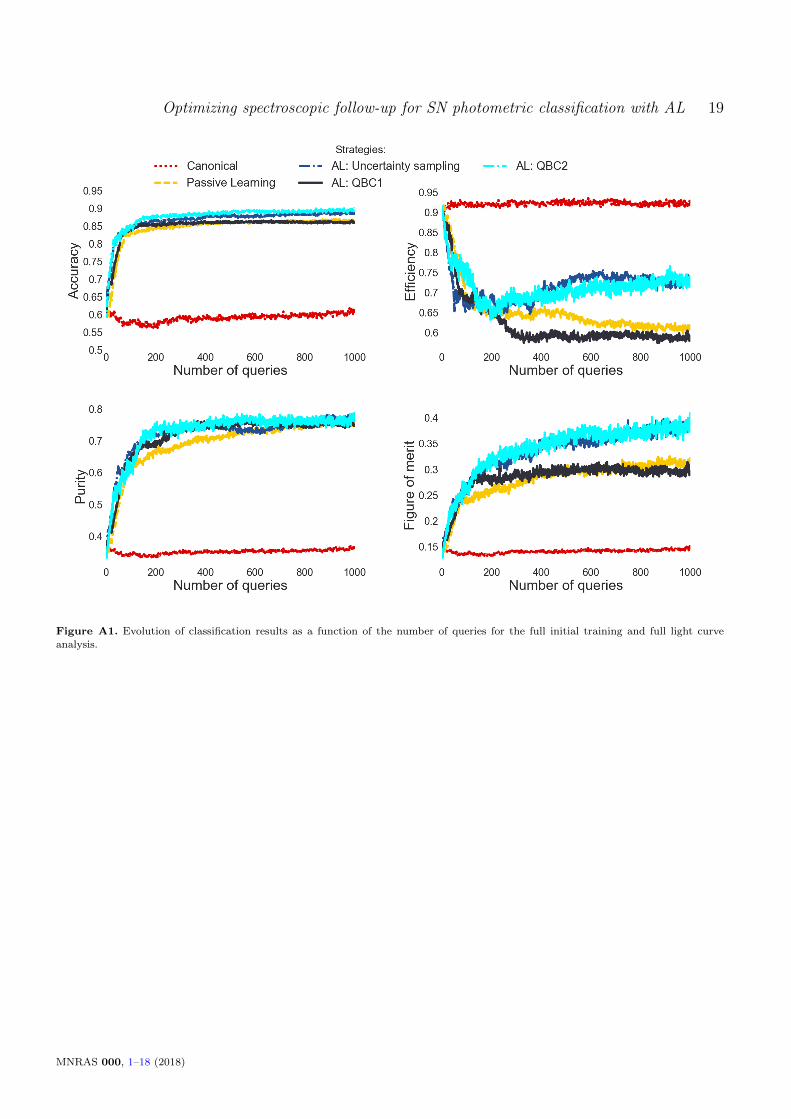
Optimizing spectroscopic follow-up for SN photometric classification with AL 19

Figure A1. Evolution of classification results as a function of the number of queries for the full initial training and full light curve

analysis.

MNRAS 000, 1–18 (2018)