Pontificia Universidad Catolica de Chile

Instituto de Astrofısica

Facultad de Fısica

Supernovae Rate in RCS-2 Fields

by

Josefina Michea Karmelic.

Practice report presented to the Physics Faculty of Pontificia

Universidad Catolica de Chile, as one of the requirements for the

Bachelor degree in Astronomy.

Supervisor : Dr. Luis Felipe Barrientos

Correctors : Dr. Timo Anguita

: Dr. Alejandro Clocchiatti

July, 2013

Santiago – Chile

Abstract

Blah

2

Contents

1 Introduction 9

1.1 Type Ia Supernovae . . . . . . . . . . . . . . . . . . . . . . . . . . . . . . . 10

1.2 Supernovae Rates . . . . . . . . . . . . . . . . . . . . . . . . . . . . . . . . 12

1.3 The Red-Sequence Cluster Survey 2 . . . . . . . . . . . . . . . . . . . . . . 12

1.3.1 LRG Selection . . . . . . . . . . . . . . . . . . . . . . . . . . . . . . 13

1.3.2 Expected Number of Supernovae . . . . . . . . . . . . . . . . . . . 13

2 Working with the Data 14

2.1 Constructing the Difference Images . . . . . . . . . . . . . . . . . . . . . . 14

2.1.1 Galaxy Stamps . . . . . . . . . . . . . . . . . . . . . . . . . . . . . 14

2.1.2 Cosmic Ray Removal . . . . . . . . . . . . . . . . . . . . . . . . . . 15

2.1.3 Sky Level Subtraction . . . . . . . . . . . . . . . . . . . . . . . . . 15

2.1.4 Convolution . . . . . . . . . . . . . . . . . . . . . . . . . . . . . . . 16

2.1.5 Galaxy Center Determination . . . . . . . . . . . . . . . . . . . . . 19

2.1.6 Image Shifting . . . . . . . . . . . . . . . . . . . . . . . . . . . . . . 21

2.1.7 Image Subtraction . . . . . . . . . . . . . . . . . . . . . . . . . . . 22

2.2 Running SExtractor . . . . . . . . . . . . . . . . . . . . . . . . . . . . . . 24

2.2.1 Configuration and Parameters . . . . . . . . . . . . . . . . . . . . . 24

4

2.2.2 Constructing a Catalog of Candidates . . . . . . . . . . . . . . . . . 25

2.2.3 Visual Checking for Supernovae . . . . . . . . . . . . . . . . . . . . 31

3 Results 32

3.1 Detected Supernovae . . . . . . . . . . . . . . . . . . . . . . . . . . . . . . 32

3.2 Supernovae Rate Calculation . . . . . . . . . . . . . . . . . . . . . . . . . . 39

3.2.1 Redshift Distribution . . . . . . . . . . . . . . . . . . . . . . . . . . 40

3.2.2 Type Ia SN Light Curve . . . . . . . . . . . . . . . . . . . . . . . . 41

3.2.3 Supernovae Rate . . . . . . . . . . . . . . . . . . . . . . . . . . . . 43

4 Conclusions and Future Work 45

5 References 46

6 Appendix 48

6.1 Convolving Data with Gaussian Distributions . . . . . . . . . . . . . . . . 48

6.1.1 Convolution Theorem . . . . . . . . . . . . . . . . . . . . . . . . . . 48

6.1.2 Fourier Transform of a Gaussian Distribution . . . . . . . . . . . . 48

6.1.3 Convolving and Deconvolving . . . . . . . . . . . . . . . . . . . . . 50

5

Figure Index

2.1 The full width at half maximum of a gaussian distribution . . . . . . . . . 17

2.2 Determination of the central position of a galaxy . . . . . . . . . . . . . . 20

2.3 The field in a cutout LRG image . . . . . . . . . . . . . . . . . . . . . . . 21

2.4 Example of the difference image of a LRG . . . . . . . . . . . . . . . . . . 23

2.5 Histogram: residuals’ distance to the center of their galaxy . . . . . . . . . 26

2.6 Contour plots: ellipticity versus flux of the residuals . . . . . . . . . . . . . 28

2.7 r-i contour plots: ellipticity versus flux of the preliminar candidates at

different radii from the center . . . . . . . . . . . . . . . . . . . . . . . . . 29

2.8 i-r contour plots: ellipticity versus flux of the preliminar candidates at

different radii from the center . . . . . . . . . . . . . . . . . . . . . . . . . 30

3.1 Histogram: SNe’s distance to the center of their galaxy . . . . . . . . . . . 34

3.2 Supernovae images . . . . . . . . . . . . . . . . . . . . . . . . . . . . . . . 39

3.3 Histogram: redshift distribution of the LRGs in the catalog . . . . . . . . . 40

3.4 Light curve in the r band of the supernova SNLS-04D3fk . . . . . . . . . . 42

6

Table Index

3.1 LRGs that host SNe . . . . . . . . . . . . . . . . . . . . . . . . . . . . . . 33

7

Chapter 1

Introduction

LRGs: Most luminous galaxies in clusters are a very homogeneous population. Very

narrow range of color and intrinsic luminosity. Because these objects are intrinsically

very luminous, they can be observed to great distance.

Motivation: Why SNe in LRGs?

SNe Ia rate is much lower in ellipticals compared to spirals –¿ less SNe occurr in

ellipticals; less motivation to study elliptical rates.

It is difficult to find SNe at high redshift. Generally, spectroscopy can’t be done to

the hosting galaxy; not seen, too far away –¿ cannot know the redshift.

Elliptical galaxies -¿ found in clusters. In the case of finding a SNe in a galaxy that

belongs to a cluster, spectroscopy can be done to the brightest member of the cluster –¿

we can know the redshift. No dust!!!

Specifically LRGs: the brightest, most massive elliptical galaxies in clusters.

High redshift SNe =¿ Cosmological interest. We can determine distances to constrain

cosmological parameters -¿ accelerating expanding universe.

9

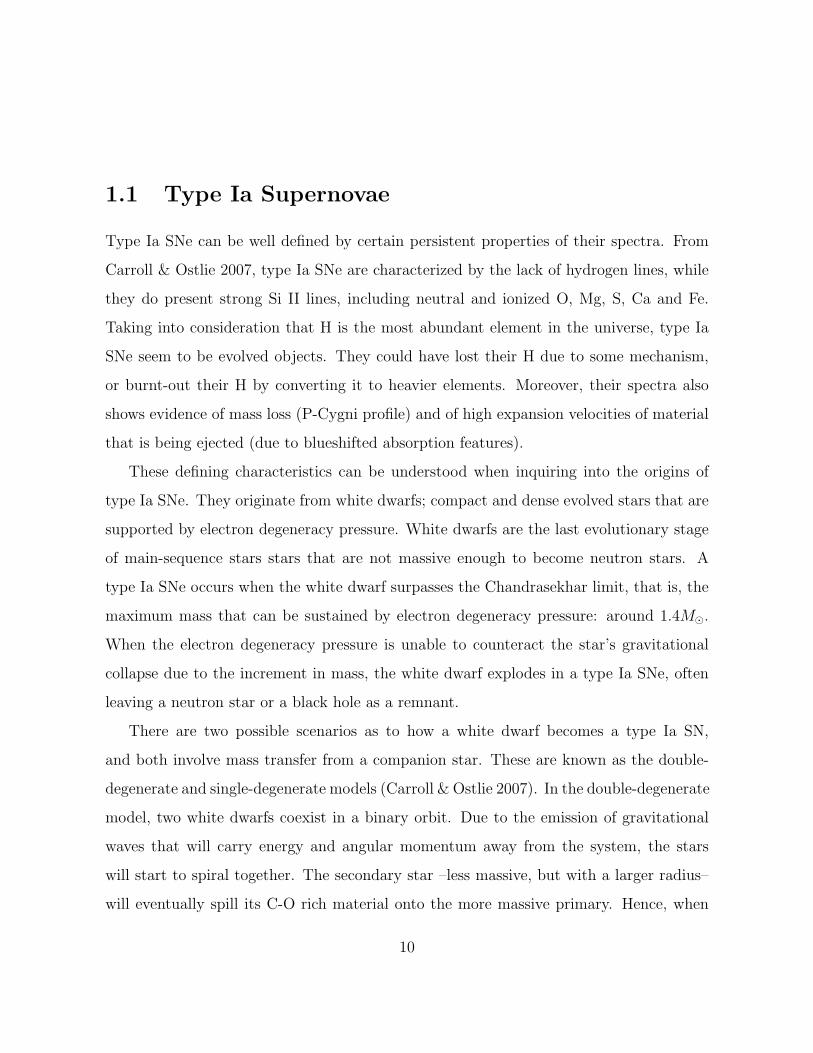
1.1 Type Ia Supernovae

Type Ia SNe can be well defined by certain persistent properties of their spectra. From

Carroll & Ostlie 2007, type Ia SNe are characterized by the lack of hydrogen lines, while

they do present strong Si II lines, including neutral and ionized O, Mg, S, Ca and Fe.

Taking into consideration that H is the most abundant element in the universe, type Ia

SNe seem to be evolved objects. They could have lost their H due to some mechanism,

or burnt-out their H by converting it to heavier elements. Moreover, their spectra also

shows evidence of mass loss (P-Cygni profile) and of high expansion velocities of material

that is being ejected (due to blueshifted absorption features).

These defining characteristics can be understood when inquiring into the origins of

type Ia SNe. They originate from white dwarfs; compact and dense evolved stars that are

supported by electron degeneracy pressure. White dwarfs are the last evolutionary stage

of main-sequence stars stars that are not massive enough to become neutron stars. A

type Ia SNe occurs when the white dwarf surpasses the Chandrasekhar limit, that is, the

maximum mass that can be sustained by electron degeneracy pressure: around 1.4M�.

When the electron degeneracy pressure is unable to counteract the star’s gravitational

collapse due to the increment in mass, the white dwarf explodes in a type Ia SNe, often

leaving a neutron star or a black hole as a remnant.

There are two possible scenarios as to how a white dwarf becomes a type Ia SN,

and both involve mass transfer from a companion star. These are known as the double-

degenerate and single-degenerate models (Carroll & Ostlie 2007). In the double-degenerate

model, two white dwarfs coexist in a binary orbit. Due to the emission of gravitational

waves that will carry energy and angular momentum away from the system, the stars

will start to spiral together. The secondary star –less massive, but with a larger radius–

will eventually spill its C-O rich material onto the more massive primary. Hence, when

10

the primary star surpasses the Chandrasekhar limit, it will explode into a type Ia SNe.

On the other hand, the single-degenerate model consists of an evolving star and a white

dwarf in a binary orbit. What exactly happens with the non-degenerate material that

spills from the evolving star onto the white dwarf is uncertain. An option is that if enough

helium settles, the degenerate C-O in the center of the white dwarf could ignite, and the

degenerate gas would not longer be able to support the mass of the star. Another option is

that material is simply spilled onto the white dwarf until it surpasses the Chandrasekhar

limit. Either way, the resolution is a type Ia SN.

Type Ia SNe are present in both passive galaxies (ellipticals, like LRGs) and star-

forming galaxies (spirals and irregulars). Notwithstanding, types Ib, Ic, II SNe have only

been observed in star-forming regions where formation of massive stars has taken place.

These SNe types consist of core-collapse events, in which massive stars evolve, become

degenerate and surpass the Chandrasekhar limit.

Elliptical galaxies show little evidence of recent star-formation activity, and are con-

stituted by older, low-mass stars. Therefore, the only kind of SNe that can be found on

LRGs are types Ia.

Type Ia SNe are consistent events. Their maximum energy output varies within a

small and constrained magnitude range. Moreover, there is a relationship between the

peak brightness and the rate of decline of their light curve, in which the light of the most

energetic SNe declines slower (Carroll & Ostlie 2007). Therefore, an orderly progression

from the most-luminous and slowest-declining events to the less-luminous and fastest-

declining events can be established and studied (Hamuy et al. 1996). This level of

consistency makes type Ia SNe an ideal tool to study the universe: they can be used to

constrain cosmological parameters, and ultimately probe the structure of the universe to

great distances (Leibundgut 2008).

11

1.2 Supernovae Rates

There is a very small n of sne known in elliptical galaxies, and the statistics are very

uncertain –¡ motivation! ()

In literature. - approx 20-30 times bigger in later galaxies.

1.3 The Red-Sequence Cluster Survey 2

The second Red-sequence Cluster Survey (RCS-2)

Red-sequence Cluster Survey sample of galaxy clusters optically selected. Method:

cores of galaxy clusters are dominated by galaxies with old stellar populations, form-

ing a tight red-sequence in color magnitude space -¿ red-sequence based cluster finding

algorithms.

Square degree imager, Megacam, with wide-field imager capabilities installed on the

3.6 m Canada-France-Hawaii Telescope (CFHT).

(Gilbank et al. 2011).

- 1 pixel corresponds to 0.185 arcseconds. - The g, r, and z filter imaging is done under

a same observation, while i filter imaging is incorporated later. Only around 70% of the

survey is i filter covered.

*poner grafico tiempo i-r, pedir al profesor.

For our time variability study, we are interested either in the g, r or z filter image and

in the i filter image, which is taken one year later in average. We will be using filter r

(*because...).

12

1.3.1 LRG Selection

LRGs are selected from the RCS-2 object catalog using a color criteria. (*Which is...:).

This results in a selection of 62812 galaxies.

From the preliminary galaxy selection, LRGs must meet certain requirements to be

of use for this study. First, galaxies that were not covered by i filter imaging are of no

use, and therefore are discarded. Approximately a 72.8% (45751) from our initial 62812

galaxies have i filter images. Second, the specific pointings of the fields in which our

galaxies appear must have had their seeing measured. This is necessary for a later step

in the data analysis, detailed in section 2.1.4. While all objects had their observation

seeing measured during the r filter imaging, some i filter imaging has no information on

the seeing of their night. This narrows our LRG catalog to 36070 objects, and for each

one we have the following essential information:

→ the patch in which the galaxy is found,

→ its coordinates (right ascension and declination), and

→ the seeing of the specific pointing in which the galaxy was observed, in terms of the

FWHM of a point source (for both the r and i filters).

1.3.2 Expected Number of Supernovae

Based on SNe rates in literature. As they were taken with a year difference in average,

sn could occurr in r or in i.

13

Chapter 2

Working with the Data

2.1 Constructing the Difference Images

2.1.1 Galaxy Stamps

The first step is to access the RCS-2 patches and make cutouts of the LRGs in the

constructed catalog. This is done using a script designed for this purpose by Dr. Luis

Felipe Barrientos. By providing the right ascension and declination of each galaxy, an

approximate size of the desired aperture and an outname, the script makes precise cutouts

from the r and the i filter pointings.

Apertures of about 0.3 arcminutes were considered to be suficient to cover up the

galaxies’ span on the sky. This results in r and i filter images of dimensions 89×89

pixels for each LRG –which correspond, more precisely, to an aperture of 0.274×0.274

arcminutes centered on the galaxy–.

14

2.1.2 Cosmic Ray Removal

A first look through the r and i filter images of the LRGs shows that they are not cosmic

ray clean. High-energy charged particles –mostly protons– originating from sources like

quasars, SNe, active galactic nuclei and magnetic variable stars penetrate the Earth’s

atmosphere and hit the CCD chips directly; not necessarily passing through the telescope.

Due to their high energies they leave very bright, sharp dots or trails on the pixel (or pixels)

on which they land.

Cosmic rays contaminate the science images and, if not removed, could eventually lead

to wrong conclusions –for example, by confusing them with SNe–. We use the Laplacian

Cosmic Ray Identification (L.A.Cosmic) program written by Pieter G. van Dokkum (van

Dokkum 2001) to clean the images from cosmic rays. The algorithm distinguishes between

poor sampled sources and cosmic rays, identifying them based on their brightness and the

sharpness of their edges.

Using the lacos im task in the IRAF (Image Reduction and Analysis Facility) soft-

ware, we clean the r and i filter image of each galaxy from cosmic rays. As a precaution,

the parameter that assigns the number of iterations of the algorithm over an image (niter)

is set to 1, so that, primarily, the most evident cosmic rays are removed. Hopefully, this

yields a smaller risk of affecting possible SNe.

2.1.3 Sky Level Subtraction

The r and i filter images of each galaxy have different sky levels. As we wish to make the

different filter images comparable, it is necessary to equate these values. This is done by

determining the sky level from each image and then subtracting it, leaving a baseline sky

value bordering zero.

15

As the galaxies are positioned relatively at the center of their cutouts, it can be

assumed that the sky begins at a certain radius –the boundaries of the galaxy– and

extends towards the borders of the image. If we suppose that LRGs have a typical size

in the sky of 10 arcseconds, then a central aperture of 50 pixels in diameter is enough

to cover up the extension of most galaxies. Therefore, by applying a circular mask of 50

pixels in diameter at the center of each r and i filter image, we compute the median to

the pixels that lie beyond the mask –which are considered to represent the sky–. This

median sky value is then subtracted to the whole image.

2.1.4 Convolution

The observations in which we find our galaxies were taken in an extended period of time

–throughout different nights–; therefore, each pointing ocurred under different atmospher-

ical conditions. Factors like the turbulence of the Earth’s atmosphere and the humidity

level of a night define the astronomical seeing of an observation. The lower the seeing

value, the better the quality of the data attained. The seeing makes the response of an

astronomical instrument to a light source a variable factor in time.

Moreover, point sources –like stars– detected by a telescope are not captured by the

ccd as points; instead, they occupy a certain area that is dependent on the instrumental

properties of the telescope and the specific seeing under which the observation takes place.

This response of an imaging system to a light source is characterized by a point spread

function (PSF).

As the observations using the r and i filters took place in separate time spans, each

LRG has a characteristic PSF in its r filter image and in its i filter image. To quantify

the difference in the PSFs of a galaxy in each filter, we take into consideration the full

width at half maximum (FWHM) of the gaussian distribution of a point source present in

16

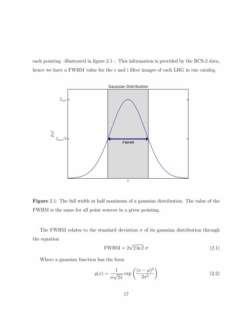
each pointing –illustrated in figure 2.1–. This information is provided by the RCS-2 data,

hence we have a FWHM value for the r and i filter images of each LRG in our catalog.

x

fmax/2

fmax

f(x)

FWHM

Gaussian Distribution

Figure 2.1: The full width at half maximum of a gaussian distribution. The value of the

FWHM is the same for all point sources in a given pointing.

The FWHM relates to the standard deviation σ of its gaussian distribution through

the equation

FWHM = 2√2 ln 2 σ (2.1)

Where a gaussian function has the form

g(x) =1

σ√2π

exp

((x− µ)2

2σ2

)(2.2)

17

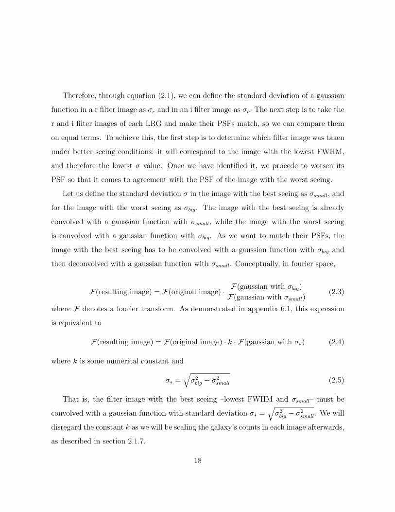
Therefore, through equation (2.1), we can define the standard deviation of a gaussian

function in a r filter image as σr and in an i filter image as σi. The next step is to take the

r and i filter images of each LRG and make their PSFs match, so we can compare them

on equal terms. To achieve this, the first step is to determine which filter image was taken

under better seeing conditions: it will correspond to the image with the lowest FWHM,

and therefore the lowest σ value. Once we have identified it, we procede to worsen its

PSF so that it comes to agreement with the PSF of the image with the worst seeing.

Let us define the standard deviation σ in the image with the best seeing as σsmall, and

for the image with the worst seeing as σbig. The image with the best seeing is already

convolved with a gaussian function with σsmall, while the image with the worst seeing

is convolved with a gaussian function with σbig. As we want to match their PSFs, the

image with the best seeing has to be convolved with a gaussian function with σbig and

then deconvolved with a gaussian function with σsmall. Conceptually, in fourier space,

F(resulting image) = F(original image) · F(gaussian with σbig)

F(gaussian with σsmall)(2.3)

where F denotes a fourier transform. As demonstrated in appendix 6.1, this expression

is equivalent to

F(resulting image) = F(original image) · k · F(gaussian with σ∗) (2.4)

where k is some numerical constant and

σ∗ =√σ2big − σ2

small (2.5)

That is, the filter image with the best seeing –lowest FWHM and σsmall– must be

convolved with a gaussian function with standard deviation σ∗ =√

σ2big − σ2

small. We will

disregard the constant k as we will be scaling the galaxy’s counts in each image afterwards,

as described in section 2.1.7.

18

In summary, for each LRG in our catalog, we first examine the FWHM values of their r

and i images, then calculate the σbig and σsmall values (equation (2.1)) to determine which

of the two images will have to be convolved, and finally compute the standard deviation

σ∗ (equation (2.5)). The convolution between the image with the lowest FHWM value

and a gaussian function with σ∗ is done using the gauss task in IRAF, located in the

images.imfilter package.

2.1.5 Galaxy Center Determination

The galaxy cutouts were generated with the LRGs relatively at the center of their image.

However, if we want to do difference imaging, it is imperative for the galaxies to accurately

share a central position on their r and i filter images. Therefore, the first step is to

determine with precision the central pixel coordinates (xc, yc) of each LRG in both of its

images, so they can be aligned afterwards (as described later in section 2.1.6).

For each pixel position, we have its coordinates (x, y) and a given number of counts

z = f(x, y). We assume the galactic center (xc, yc) will correspond to the position with the

highest number of counts. To determine the center, we interpolate adjacent pixel values

to create a smooth, two dimensional surface that can be evaluated at any position. By

implementing in Python the RectBivariateSpline class in scipy.interpolate,

we use cubic spline interpolation to create a smooth 2D function based on our fixed data

points. Then, we can accurately determine the central coordinates of the LRGs based on

an apperture of 20×20 pixels positioned at the center of the image. The interpolation

procedure is illustrated in figure 2.2.

It is important to note that finding a central position value is problematic when there

are several objects on the cutout field. As the galaxies differ –sometimes more subtly and

sometimes more significantly– in their position on the r and i filter images, the object(s)

19

35

40

45

50

Original Interpolated

35 40 45 5035

40

45

50

35 40 45 50

Figure 2.2: Determination of the central position of a galaxy, by interpolating the data

points in a 20×20 pixel sized apperture. (Left) The original image, displayed also as a

2D countour plot. (Right) The interpolated image, where the central coordinates of the

galaxy have been determined and are indicated by the intersection of two lines.

on the field also shift in and out of the image. Given the case that they are brighter

than the LRG and appear al least partially in one of the appertures (r or i), they can

perjudicially influence the center determination. Therefore, the galaxies’ central position

is, generally, best determined when the central area of the LRGs have no other objects

around –see figure 2.3–.

20

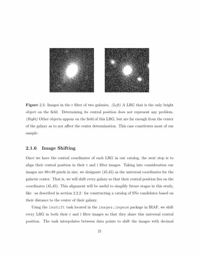
Figure 2.3: Images in the r filter of two galaxies. (Left) A LRG that is the only bright

object on the field. Determining its central position does not represent any problem.

(Right) Other objects appear on the field of this LRG, but are far enough from the center

of the galaxy as to not affect the center determination. This case constitutes most of our

sample.

2.1.6 Image Shifting

Once we have the central coordinates of each LRG in our catalog, the next step is to

align their central position in their r and i filter images. Taking into consideration our

images are 89×89 pixels in size, we designate (45,45) as the universal coordinates for the

galactic center. That is, we will shift every galaxy so that their central position lies on the

coordinates (45,45). This alignment will be useful to simplify future stages in this study,

like –as described in section 2.2.2– for constructing a catalog of SNe candidates based on

their distance to the center of their galaxy.

Using the imshift task located in the images.imgeom package in IRAF, we shift

every LRG in both their r and i filter images so that they share this universal central

position. The task interpolates between data points to shift the images with decimal

21

precision.

2.1.7 Image Subtraction

To finally create the difference images, each galaxy’s counts have to be scaled so that they

match in their r and i filter image. By positioning 5×5 pixel appertures at the center

of each LRG, we are able to determine the median number of counts. This allows us to

compute a scale factor between each r and i filter image. Conceptually, if we want the r-i

difference image, then

r-i image = r− sr−i · i (2.6)

where the scale factor

sr−i =r median 5×5

i median 5×5

(2.7)

Therefore, we are scaling the i filter image to match the counts of the r filter image. If

we are interested in the i-r difference image, then we scale the r filter image:

i-r image = i− si−r · r (2.8)

where

si−r =i median 5×5

r median 5×5

(2.9)

This way, the objects that are detected in the difference images will have authentic –not

scaled– number of counts. As we will be later running the SExtractor (Source Extractor)

program over the difference images to build a catalog of possible SNe (see section 2.2), we

are interested in both the r-i and i-r difference images. SExtractor is not able to detect

negative counts as an object.

The process of difference imaging for one galaxy is illustrated in figure 2.4. It can be

observed that the subtracted images have residuals at the center. This is the case in most

22

–if not all– of our difference images. Our scaling technique based on the median value

of the central area of the galaxies is probably too rudimentary to obtain a satisfactory

subtraction at the center. Nevertheless, the difference images are successful on the areas

that lie beyond the center; towards the outskirts of the galaxy.

Figure 2.4: Example of the difference images of a LRG. (Upper row) The r filter image is

to the left, while the i filter image is to the right. Note that the r filter image looks more

blurry or softened than its counterpart because it was, in this particular case, the image

that had to be convolved with a gaussian to worsen its PSF and match the i filter image

quality. (Lower row) The difference images, r-i to the left and i-r to the right. Except

from the scaling, one is the negative of the other. The other objects present on the field

will often leave residuals, as the scaling done is only focused in subtracting correctly the

LRG.

23

2.2 Running SExtractor

Once we have created the r-i and i-r difference images for all the LRGs in our catalog,

the next step is to run the SExtractor program over them to detect possible objects, and

construct a catalog of SNe candidates.

2.2.1 Configuration and Parameters

The SExtractor configuration file is adapted so that the program runs suiting the needs of

this study. The most relevant change that is done to the default settings is the inclusion

of weight maps. The background noise level in an astronomical image is generally fairly

constant but, given the case there are noise peaks in some areas, the process of object

detection will be impaired. Therefore, we create background noise maps of each difference

image as to inform SExtractor of the noise intensity at each pixel.

The subtraction of r-i and i-r to construct the difference images means that we are

adding up the noise level of each individual image into a new image. Moreover, if we

wish to quantify the background noise, we need to add back the sky level values that were

subtracted previously (see section 2.1.3). This allows us to retreive the original weight of

each pixel. For the r-i and i-r difference images we define, respectively, their weight maps

as follows:

Wr-i = median filter 5×5

[(r+skyr) + sr−i · (i+skyi)

](2.10)

Wi-r = median filter 5×5

[(i+skyi) + si−r · (r+skyr)

](2.11)

24

The data is median filtered in 5×5 pixel sized appertures. That is, each pixel value is

smoothed out based on the median value of the surrounding pixels. The median filtering

is done in Python, using the median filter class in scipy.ndimage.filters.

The next step is to decide what do we wish to know from the objects detected by SEx-

tractor. Considering we want to find SNe candidates, the essential parameters correspond

to:

→ The pixel coordinates of the residual (X IMAGE and Y IMAGE parameters).

→ The flux of the residual and its associated uncertainty (FLUX AUTO and

FLUXERR AUTO parameters.)

→ The ellipticity of the residual (ELLIPTICITY parameter).

→ The FWHM of the residual (FWHM IMAGE parameter).

The choice of these parameters is later justified by the use we give them in section 2.2.2.

Finally running SExtractor over the difference images, we end up with a catalog consti-

tuted of 92939 possible objects from r-i and 76414 possible objects from i-r images.

2.2.2 Constructing a Catalog of Candidates

Filtering criteria must be established to discriminate in our catalog which possible objects

could be SNe candidates. We create diagnostic plots to decide how to constrain the

catalog.

For a first approach, we map the spatial distribution of the residuals in respect to the

center of their galaxy. By assuming all LRGs are spherical in shape –a simplification–,

we define the modulus distance d to the center using Pythagoras’ theorem:

d =√

(x− xc)2 + (y − yc)2 (2.12)

25

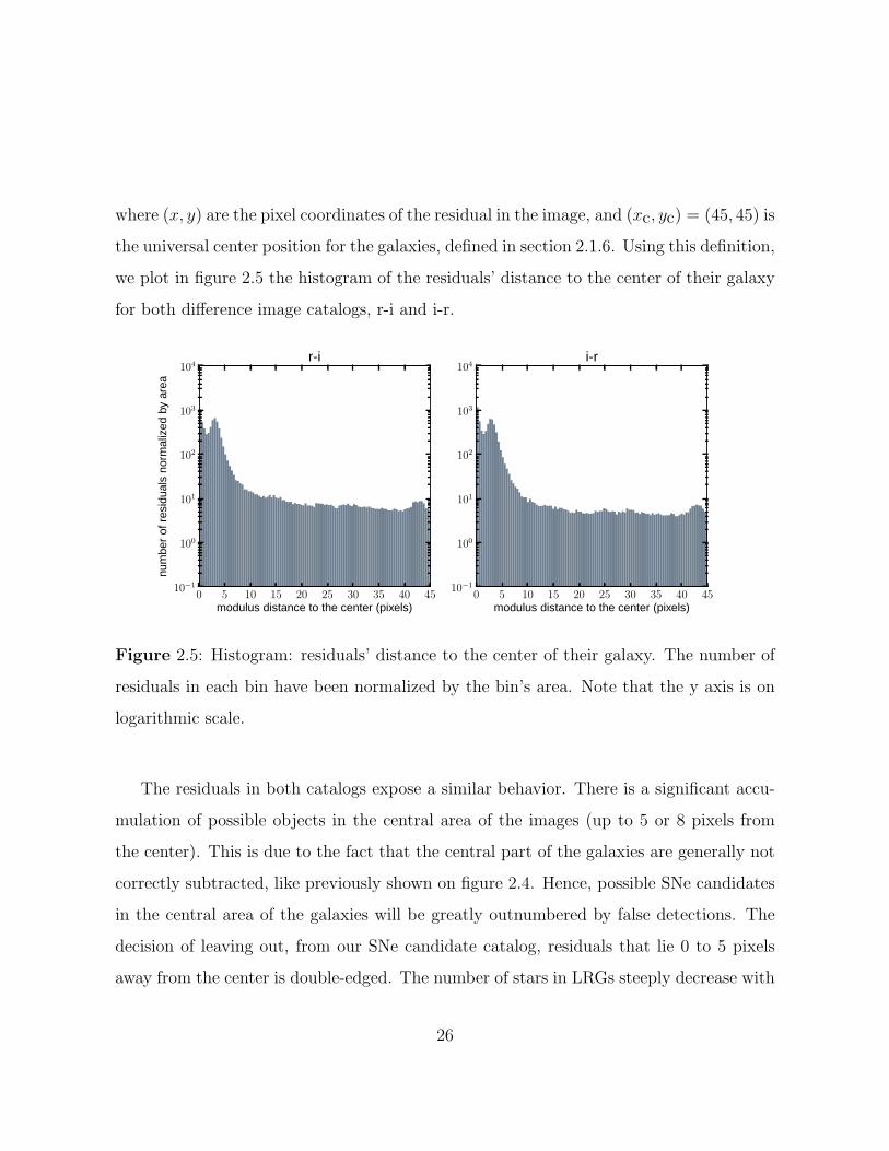
where (x, y) are the pixel coordinates of the residual in the image, and (xc, yc) = (45, 45) is

the universal center position for the galaxies, defined in section 2.1.6. Using this definition,

we plot in figure 2.5 the histogram of the residuals’ distance to the center of their galaxy

for both difference image catalogs, r-i and i-r.

0 5 10 15 20 25 30 35 40 45

modulus distance to the center (pixels)

10−1

100

101

102

103

104

num

ber

ofre

sidu

als

norm

aliz

edby

area

r-i

0 5 10 15 20 25 30 35 40 45

modulus distance to the center (pixels)

10−1

100

101

102

103

104

i-r

Figure 2.5: Histogram: residuals’ distance to the center of their galaxy. The number of

residuals in each bin have been normalized by the bin’s area. Note that the y axis is on

logarithmic scale.

The residuals in both catalogs expose a similar behavior. There is a significant accu-

mulation of possible objects in the central area of the images (up to 5 or 8 pixels from

the center). This is due to the fact that the central part of the galaxies are generally not

correctly subtracted, like previously shown on figure 2.4. Hence, possible SNe candidates

in the central area of the galaxies will be greatly outnumbered by false detections. The

decision of leaving out, from our SNe candidate catalog, residuals that lie 0 to 5 pixels

away from the center is double-edged. The number of stars in LRGs steeply decrease with

26

the distance to the center of the galaxy –elliptical galaxies have a de Vaucouleurs profile–.

Therefore, under the assumption that more stars mean more possibilities of a type Ia SN

occurring, we are cutting out the pixel range with highest probability of sheltering SNe.

Despite this, we will omit the central area as it is too deeply contamined.

The decreasing number of residuals with the distance to the center ends with a small

peak towards d = 40 pixels. This behavior could be illustrating another area that is high

in contaminant residuals.

Another diagnostic plot is the ellipticity versus the flux of the residuals in both r-i and

i-r catalogs, shown in figure 2.6. The ellipticity e of the residuals is defined as

e = 1− b

a(2.13)

where b corresponds to the semi-minor axis and a to the semi-major axis length. Therefore,

the more rounded residuals are the ones with a smaller e value. As stars are spherical

objects, we could expect SNe to be observed approximately spherical as well, assuming

that the explosion is relatively isotropic.

We can observe that the distribution concentrates around e = 0.4 with a span between

the 103 to 104 flux values. There is also a high flux and highly elliptical group, most likely

dominated by contaminants. As we are unsure about the possible brightness range of SNe

in our images –the flux values are not calibrated–, we decide to only cut by ellipticity.

To elude the concentration at e = 0.4, probably constituted by the high number of

contaminants in the central area, we decide to search for SNe at ellipticities below e = 0.2.

Another parameter we take into consideration to constrain our sample is the FWHM

of the residuals. We had added in the configuration file of SExtractor that starlike objects

would have a FWHM of around 4 pixels. Based on this conjecture, and considering that

SNe are not very extended objects, we impose FWHM < 10 pixels for our SNe candidates.

27

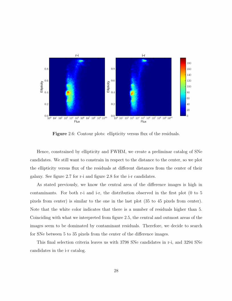
Figure 2.6: Contour plots: ellipticity versus flux of the residuals.

Hence, constrained by ellipticity and FWHM, we create a preliminar catalog of SNe

candidates. We still want to constrain in respect to the distance to the center, so we plot

the ellipticity versus flux of the residuals at different distances from the center of their

galaxy. See figure 2.7 for r-i and figure 2.8 for the i-r candidates.

As stated previously, we know the central area of the difference images is high in

contaminants. For both r-i and i-r, the distribution observed in the first plot (0 to 5

pixels from center) is similar to the one in the last plot (35 to 45 pixels from center).

Note that the white color indicates that there is a number of residuals higher than 5.

Coinciding with what we interpreted from figure 2.5, the central and outmost areas of the

images seem to be dominated by contaminant residuals. Therefore, we decide to search

for SNe between 5 to 35 pixels from the center of the difference images.

This final selection criteria leaves us with 3798 SNe candidates in r-i, and 3294 SNe

candidates in the i-r catalog.

28

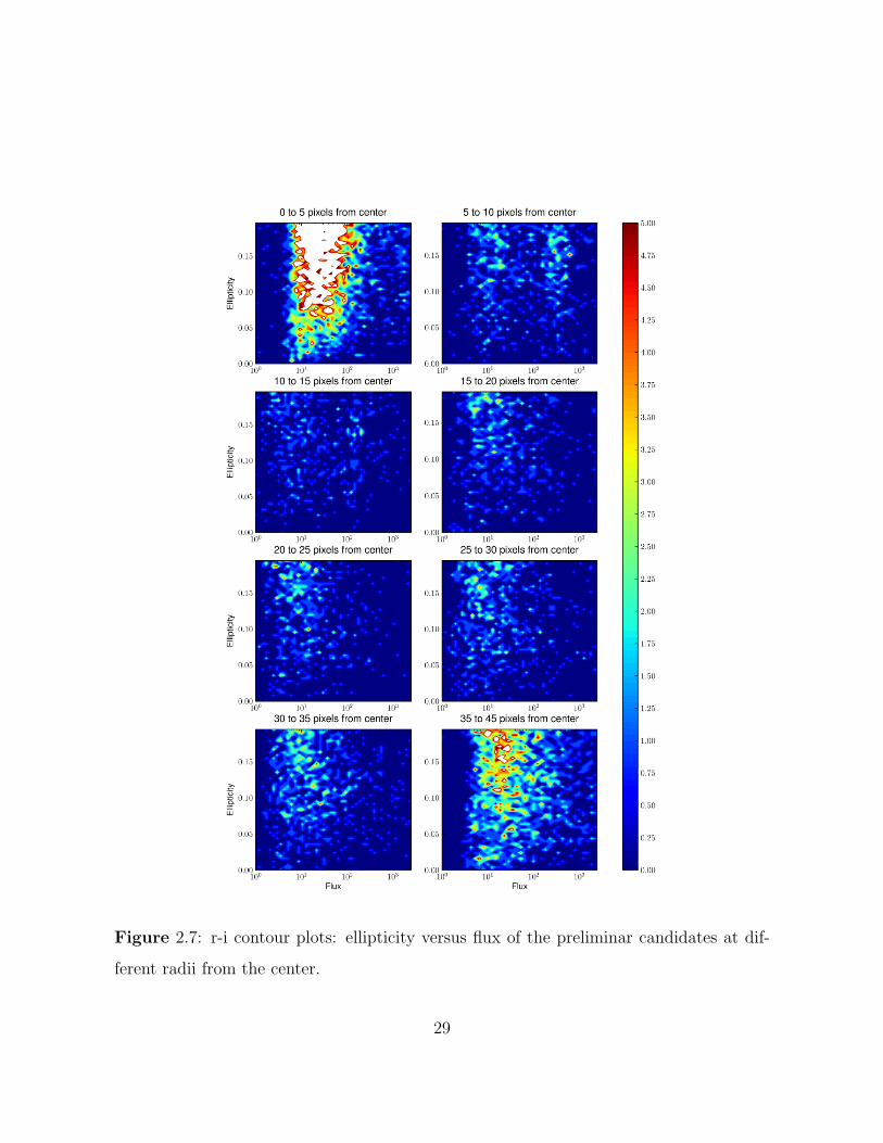
Figure 2.7: r-i contour plots: ellipticity versus flux of the preliminar candidates at dif-

ferent radii from the center.

29

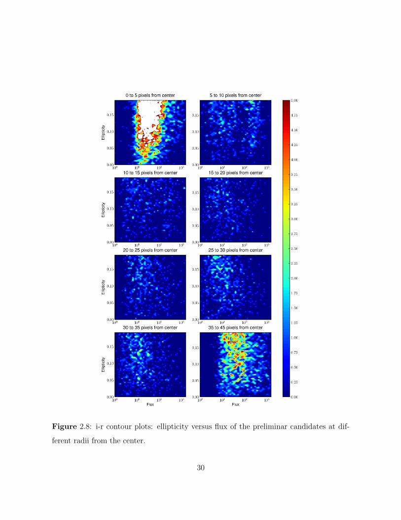
Figure 2.8: i-r contour plots: ellipticity versus flux of the preliminar candidates at dif-

ferent radii from the center.

30

2.2.3 Visual Checking for Supernovae

The next step is to visual check each difference image and evaluate which candidates could

be SNe. For each LRG with a candidate, we concatenate the original r and i filter images,

the difference image and the check image that was generated by SExtractor. This allows

us to efficiently filter our catalog.

Most of our catalog was constituted by detections of field objects. As previously

stated in section 2.1.7, the scaling for the subtraction is focused in subtracting correctly

the LRG, and not the whole field. Hence, field objects generally display residual flux in

the difference image. Another common case was that either the r or i filter image would

have its objects shifted and duplicated –like a blurred out photograph–, resulting in false

detections. Finally, there were also cases of faulty columns that prevented a good galaxy

center determination and ended up as defective subtractions.

Once the possible SNe are selected from the catalog, we generate cutouts of their LRGs

in the g and z filters. This is done to further ensure that they are, in fact, SNe, and not

just objects that are r or i filter dropouts. Taking into account that the g, r and z images

were taken during a short time span while the i filter images were taken a year later in

average, we postulate that for an object to be a SNe in a r-i difference image it has to

appear in g, r, z but not in i, and the other way around if it were a SNe in a i-r difference

image. Using this method, we are able to discard several false cases we had classified as

SNe.

Our catalog of SNe ends up finally constituted by a total of 23 SNe detections; 14 in

the r filter and 9 in the i filter images.

31

Chapter 3

Results

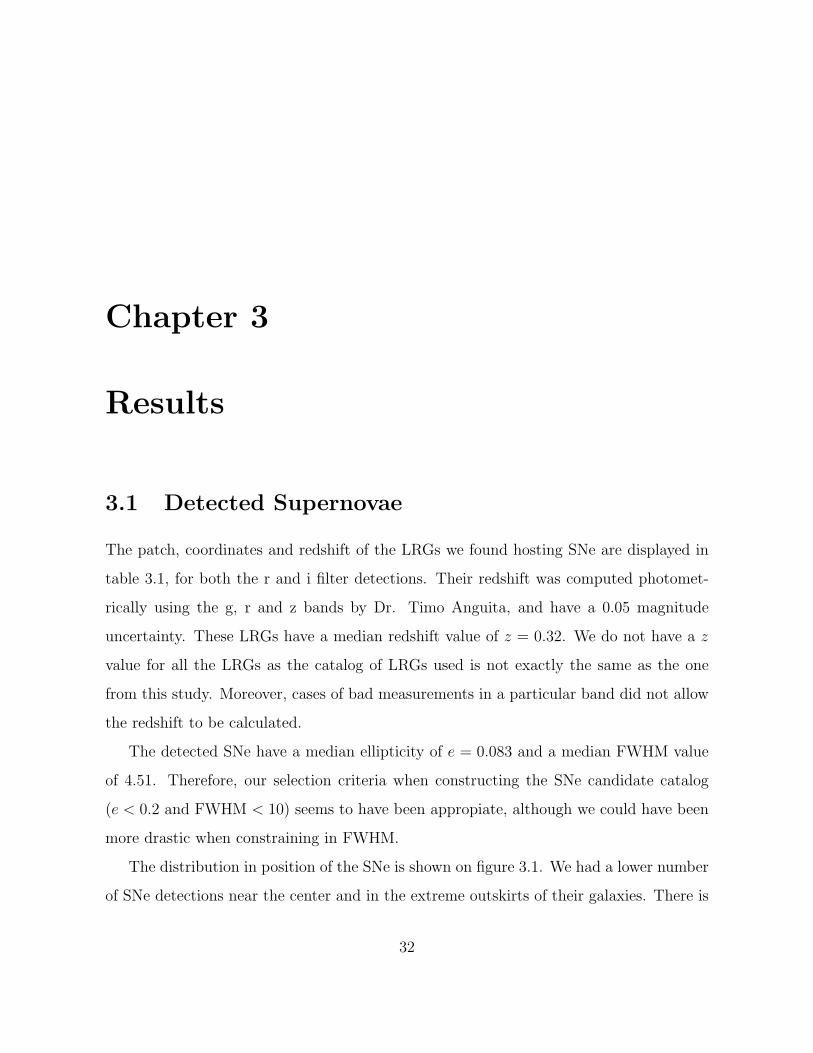
3.1 Detected Supernovae

The patch, coordinates and redshift of the LRGs we found hosting SNe are displayed in

table 3.1, for both the r and i filter detections. Their redshift was computed photomet-

rically using the g, r and z bands by Dr. Timo Anguita, and have a 0.05 magnitude

uncertainty. These LRGs have a median redshift value of z = 0.32. We do not have a z

value for all the LRGs as the catalog of LRGs used is not exactly the same as the one

from this study. Moreover, cases of bad measurements in a particular band did not allow

the redshift to be calculated.

The detected SNe have a median ellipticity of e = 0.083 and a median FWHM value

of 4.51. Therefore, our selection criteria when constructing the SNe candidate catalog

(e < 0.2 and FWHM < 10) seems to have been appropiate, although we could have been

more drastic when constraining in FWHM.

The distribution in position of the SNe is shown on figure 3.1. We had a lower number

of SNe detections near the center and in the extreme outskirts of their galaxies. There is

32

# Patch RA (hrs) DEC (deg) Redshift Filter

1 0047 0.519659 3.299874 0.39 i

2 0047 0.531798 -0.290025 0.29 i

3 0047 0.873267 1.479494 0.24 i

4 0047 0.957727 -1.967458 - r

5 0047 0.980042 -2.732310 0.25 i

6 0047 1.038171 -2.729145 - r

7 0047 1.048250 -2.282886 0.20 r

8 0133 1.365826 -1.014289 - i

9 0310 2.930305 -15.982720 0.34 r

10 0357 3.870134 -6.135403 0.37 r

11 1111 11.313188 -7.870111 - r

12 1514 15.276808 8.073701 0.32 r

13 1645 16.859076 40.226001 0.42 r

14 2143 21.385187 3.654490 0.21 i

15 2143 21.481547 4.344913 - r

16 2143 21.582887 4.128816 0.36 i

17 2143 21.750839 0.802629 0.27 i

18 2143 21.900250 -3.511255 0.22 r

19 2143 21.963124 1.353855 0.19 r

20 2329 23.348371 -0.880093 0.34 r

21 2329 23.488255 0.556918 0.36 i

22 2338 23.568833 -8.794673 0.37 r

23 2338 23.597836 -10.143852 - r

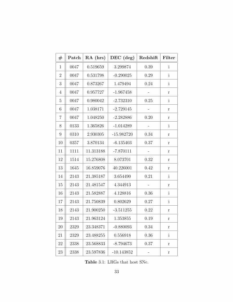
Table 3.1: LRGs that host SNe.

33

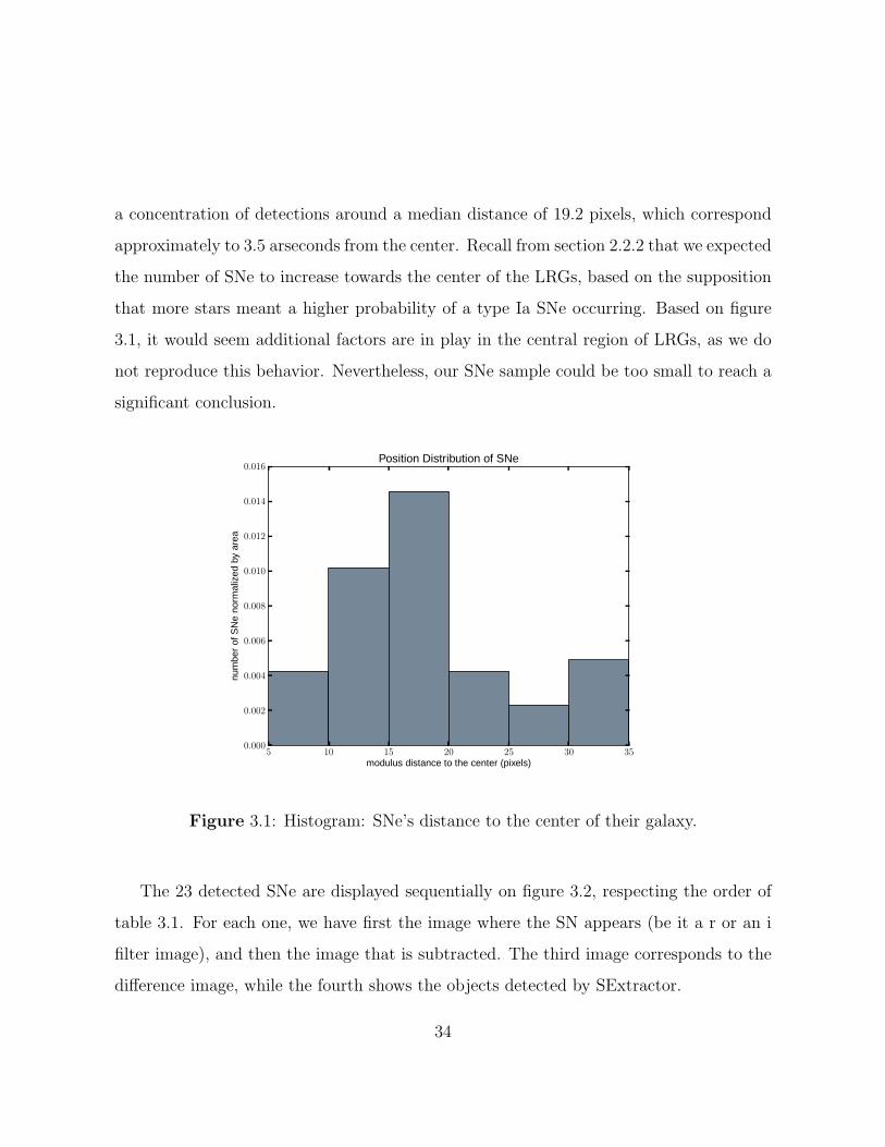
a concentration of detections around a median distance of 19.2 pixels, which correspond

approximately to 3.5 arseconds from the center. Recall from section 2.2.2 that we expected

the number of SNe to increase towards the center of the LRGs, based on the supposition

that more stars meant a higher probability of a type Ia SNe occurring. Based on figure

3.1, it would seem additional factors are in play in the central region of LRGs, as we do

not reproduce this behavior. Nevertheless, our SNe sample could be too small to reach a

significant conclusion.

5 10 15 20 25 30 35

modulus distance to the center (pixels)

0.000

0.002

0.004

0.006

0.008

0.010

0.012

0.014

0.016

num

ber

ofS

Ne

norm

aliz

edby

area

Position Distribution of SNe

Figure 3.1: Histogram: SNe’s distance to the center of their galaxy.

The 23 detected SNe are displayed sequentially on figure 3.2, respecting the order of

table 3.1. For each one, we have first the image where the SN appears (be it a r or an i

filter image), and then the image that is subtracted. The third image corresponds to the

difference image, while the fourth shows the objects detected by SExtractor.

34

35

36

37

38

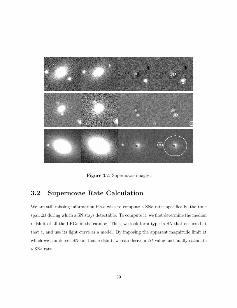
Figure 3.2: Supernovae images.

3.2 Supernovae Rate Calculation

We are still missing information if we wish to compute a SNe rate: specifically, the time

span ∆t during which a SN stays detectable. To compute it, we first determine the median

redshift of all the LRGs in the catalog. Thus, we look for a type Ia SN that occurred at

that z, and use its light curve as a model. By imposing the apparent magnitude limit at

which we can detect SNe at that redshift, we can derive a ∆t value and finally calculate

a SNe rate.

39

3.2.1 Redshift Distribution

As our LRG catalog and the catalog of LRGs that had their redshift computed have most

of their galaxies in common, we assume their redshift distributions are similar. Figure

3.3 shows that the redshift distribution of the LRGs is concentrated between z = 0.2 and

0.5, with a median redshift of 0.36. We will assume an associated uncertainty given by a

standard deviation away (1σ) from the median of the distribution.

0.0 0.2 0.4 0.6 0.8 1.0

Redshift

0

1000

2000

3000

4000

5000

6000

7000

Num

ber

ofLR

Gs

median z = 0.36

Redshift Distribution of LRGs

Figure 3.3: Histogram: redshift distribution of the LRGs in the catalog. The median

redshift is z = 0.36± 0.08.

It is preferable to employ the median redshift of all the LRGs in the catalog than just

the median redshift of the LRGs we found hosting SNe. The LRGs with SNe constitute a

small and incomplete sample, as we do not have a redshift for several cases (see table 3.1).

Moreover, as there is a magnitude limit that constrains the SNe catalog we constructed

40

–more on this on the next section–, so the fainter SNe we did not detect would not enter

in the calculation. It is safer to assume that the SNe lie around the redshift where all the

LRGs of the catalog concentrate. Therefore, we will work under the assumption that the

SNe in our LRG catalog lie around a redshift value of z = 0.36± 0.08.

3.2.2 Type Ia SN Light Curve

The light curves of SNe are affected by redshift. SNe at higher redshifts are perceived as

visible during longer periods of time; according to the theory of relativity, time is dilated

in a (1 + z) factor. This is known as cosmological time dilation, which is related to the

expansion of the universe –if a photon is emitted at redshift z, then the universe is a

factor (1 + z) bigger when it is observed–.

SNe light curves have to undertake the process of K-correction to be converted into

the rest frame. That is, our redshifted SNe would need to be blueshifted to bring them

to z = 0. Additionally, as our objects were observed through the r and i filters, only a

partial wavelength range of their total spectrum has been measured. When brought to

the rest frame, their wavelength ranges will not be corresponded, respectively, to r and i

passbands. They will fall under bluer passbands.

However, it is not necessary to engage in the complexities of K-correction, as we are

not interested in SN light curves in the rest frame. Instead, we need a type Ia SN that

occurred around redshift z = 0.36±0.08, that has not been K-corrected, and that has been

measured using r and i filters. As type Ia SNe are relatively invariant events, consistent

in the maximum energy output and the rate of decline of their light curves (see section

1.1), we can choose a particular SN light curve at z ≈ 0.36 and expect the other cases at

that z to be quite similar.

From the SuperNova Legacy Survey (SNLS, Astier et al. 2006) we choose SNLS-

41

04D3fk, a type Ia SN that occurred at z = 0.358, on which we base our calculations. The

light curve in the r band is shown in figure 3.4.

53080 53100 53120 53140 53160 53180 53200 53220

Modified Julian Date

21

22

23

24

25

26

27

28

mr

∆t ≈ 31 days

Type Ia SN Light Curve

Figure 3.4: Light curve in the r band of the supernova SNLS-04D3fk, at z = 0.358. The

light curve is fitted using cubic interpolation between data points. This basic approach is

not satisfactory for all regions of the light curve –note the bad fit towards the end–, but

works well around the peak, which is the region we are interested in.

The time span during which a SN stays visible is intertwined with our detection limit

in apparent magnitude. Although the RCS-2 has a r magnitude limit of 24.8, the actual

–and certainly brighter– limit is imposed by the magnitude of the faintest SN we visually

identified in an r filter image. This corresponds to the SN in LRG #22 in table 3.1. The

SN occurred far enough from the center of its galaxy (see its corresponding image in figure

42

3.2) as to have been detected as an object and included in the RCS-2 catalog. Hence,

photometry has been done on this particular SN, and has an r apparent magnitude of

mr = 22.84± 0.03.

However, photometric information of RCS-2 is only available in the g, r and z bands, so

we cannot determine the i magnitude of the faintest SN that occurred in an i filter image.

We will work under the assumption that the r and i passbands have similar sensibilities,

so the light curve would not vary significantly in shape.

Abiding by this magnitude limit, our model SN (figure 3.4) would have stayed de-

tectable during ∆t = 30.69± 1.81 days, where the error range is given by the uncertainty

we have in redshift. Note that this time span is already affected by time dilation, so it

corresponds to what we would observe from Earth. As previously stated, due to the lack

of i band photometry, we will consider this time span to be representative for SNe in both

r and i filter images.

3.2.3 Supernovae Rate

Finally, we have acquired all the necessary pieces to compute a type Ia SNe rate. Recapit-

ulating, from a total of 36070 LRGs, we found that 23 were hosting SNe. Consequently,

we have a factor of occurrence: (23/36070). Under the assumption that LRGs have a

typical mass of ∼ 1011M�, and that type Ia SNe at redshift z = 0.36 ± 0.08 stay visible

during a time span of ∆t = 30.69± 1.81 days,

SNR =

(23

36070

)per 1011M� per 2×∆t (3.1)

where the factor 2 affecting ∆t is due to the fact that SNe could have been detected either

in the r filter or in the i filter image. Therefore,

43

SNR =(23/36070)

2 · (30.69± 1.81) days · 1011M�(3.2)

We need to transform this rate to Supernova Units (SNu),

SNu =

[# events

century · 1010M�

](3.3)

Let us perform this transition in a logical way. First, there is a higher possibility

of finding SN in a century time span than in 2 × (30.69 ± 1.81)) days. As a century

corresponds to (365.25 · 100) days, multiplying our factor of occurrence by (365.25 · 100)

means an increase, which is conceptually correct. Second, in 1011M� there should be 10

times more SNe than in 1010M�, so we have to divide our factor of occurrence by 10.

Hence,

SNR =(23/36070) · (365.25 · 100)

2 · (30.69± 1.81) · 101

century · 1010M�(3.4)

Which finally gives us the SNe rate:

SNR = 0.038± 0.002 SNu (3.5)

** compare with snr in literature, and that’s it! :D

44

Chapter 4

Conclusions and Future Work

Difference imaging is a feasible method for finding SNe.

Future work: consider bigger sized apertures.

The assumption of section 3.2.2 is correct as a first approach (that the lc of one sne Ia

is representative of all type Ia SN at that z), but should be refined. The shape of the lc

changes based on the relation between maximum brightness and rate of decline (Hamuy

et al. 1996). The possible range of light curves should be taken into consideration when

calculating a time span of detectability.

45

Chapter 5

References

− Astier, P. et al. 2006, A&A, 447, 31

− Carroll, B. W., & Ostlie D. A. 2007, An Introduction to Modern Astrophysics (2nd

ed.; San Francisco, CA)

− Gilbank, D. G., Gladders, M. D., Yee, H. K. C., & Hsieh, B. C. 2011, AJ, 141, 94

− Hamuy, M. et al. 1996, AJ, 112, 6

− Leibundgut, B. 2008, arXiv:0802.4154

− Van Dokkum, Pieter G. 2001, PASP, 113, 1420

46

47

Chapter 6

Appendix

6.1 Convolving Data with Gaussian Distributions

6.1.1 Convolution Theorem

The convolution theorem states that

F{f ∗ g} = k · F{f} · F{g} (6.1)

where F denotes a fourier transform, and f and g are two functions with convolution

f ∗ g. The fourier transform of the convolution of two functions is then equivalent to the

product of two fourier transforms, one for each function, save a constant k that depends

on the normalization of the fourier transforms.

6.1.2 Fourier Transform of a Gaussian Distribution

Let us first take the exponential function

f(x) = exp(−x2) (6.2)

48

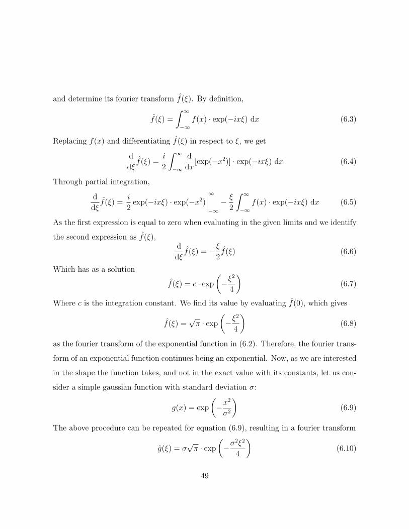
and determine its fourier transform f(ξ). By definition,

f(ξ) =

∫ ∞

−∞f(x) · exp(−ixξ) dx (6.3)

Replacing f(x) and differentiating f(ξ) in respect to ξ, we get

d

dξf(ξ) =

i

2

∫ ∞

−∞

d

dx[exp(−x2)] · exp(−ixξ) dx (6.4)

Through partial integration,

d

dξf(ξ) =

i

2exp(−ixξ) · exp(−x2)

∣∣∣∣∞−∞

− ξ

2

∫ ∞

−∞f(x) · exp(−ixξ) dx (6.5)

As the first expression is equal to zero when evaluating in the given limits and we identify

the second expression as f(ξ),d

dξf(ξ) = −ξ

2f(ξ) (6.6)

Which has as a solution

f(ξ) = c · exp(−ξ2

4

)(6.7)

Where c is the integration constant. We find its value by evaluating f(0), which gives

f(ξ) =√π · exp

(−ξ2

4

)(6.8)

as the fourier transform of the exponential function in (6.2). Therefore, the fourier trans-

form of an exponential function continues being an exponential. Now, as we are interested

in the shape the function takes, and not in the exact value with its constants, let us con-

sider a simple gaussian function with standard deviation σ:

g(x) = exp

(−x2

σ2

)(6.9)

The above procedure can be repeated for equation (6.9), resulting in a fourier transform

g(ξ) = σ√π · exp

(−σ2ξ2

4

)(6.10)

49

6.1.3 Convolving and Deconvolving

As described in section 2.1.4, once the filter image that was taken under better seeing

conditions is identified, we want to convolve it with a gaussian function of standard

deviation σbig and then deconvolve it with a gaussian function with σsmall. Reproducing

equation (2.3), in fourier space:

F(resulting image) = F(original image) · F(gaussian with σbig)

F(gaussian with σsmall)(6.11)

From equation (6.10), we know the fourier transform of a simple gaussian function.

By replacing,

F(resulting image) = F(original image) ·σbig

√π · exp

(−σ2

bigξ2

4

)σsmall

√π · exp

(−σ2

smallξ2

4

) (6.12)

Which is equivalent to

F(resulting image) = F(original image) · σbig

σsmall

· exp(−(σ2

big − σ2small)ξ

2

4

)(6.13)

Let us define

σ∗ =√σ2big − σ2

small (6.14)

Therefore, reconstructing the fourier transform of the exponential,

F(resulting image) = F(original image) · σbig

σsmall

· 1

σ∗√π· F

(exp

(−x2

σ2∗

))(6.15)

By designating the constants k, we finally obtain:

F(resulting image) = F(original image) · k · F(gaussian with σ∗) (6.16)

which is equivalent to equation (2.4). Thus, it is demonstrated that convolving the data

with a gaussian function with standard deviation σbig and then deconvolving it with a

gaussian function with σsmall is equivalent to just convolving the data with a gaussian

function with standard deviation√

σ2big − σ2

small, save from some numerical constants.

50