Embed Size (px)
Citation preview

SuperpaveAsphalt Mixture Design
WorkshopFederal Highway Administration
Version 6.4

This Workshop & Workbookdeveloped by
Thomas Harman, FHWAJohn D’Angelo, FHWAJohn Bukowski, FHWACharles Paugh, SaLUT


Foreword
n The focus of this workshop is to provide a detailed example of Superpave volumetric asphalt mixture design
1

Superpave Overview
n The final product of the SHRP asphalt program area is Superpave. Superpave is an acronym which stands for:
Superior Performing Asphalt Pavements
1

Major Steps in Superpave
n Selection of Materials,n Selection of a Design Aggregate Structure,n Selection of the Design Binder Content,andn Evaluation of Moisture Sensitivity
of the Design Mixture. SP
3

Criteria
n Environment,
n Traffic level & speed, and
n Pavement structure.
3

SIMUALTION BACKGROUND
n Location: Hot Mix, USAn Estimated, 20-year, design traffic is
6,300,000 ESAL’sn Posted traffic speed is 80 kph (50 mph)
– Estimated, ave speed is 72 kph (45 mph)
n 19.0 mm Surface Course– Such that the top of the pavement layer
from the surface is less than 100 mm.5

Update:
n All Superpave mixes are designed volumetrically.
n Currently under NCHRP study 9-19,“Superpave Models Development,”being conducted under the direction of Dr. Matt Witczak, a simple performance test is being identified/ developed.
5

A simple performance test
n Superpave mix design is volumetrically based.– Does not include a “strength test”
n NCHRP 9-19, “Superpave Support and Performance Models Program”– Dr. Matt Witczak (Arizona State University)– Dr. Ed Harrigan (NCHRP)– http://www2.nas.edu/trbcrp/

A simple performance test
nn Objective:Objective:nn To evaluate and recommend a To evaluate and recommend a
fundamentally based, but simple, fundamentally based, but simple, performance test(s) in support of performance test(s) in support of the Superpave volumetricthe Superpave volumetricmix design procedure.mix design procedure.
Spring 2000
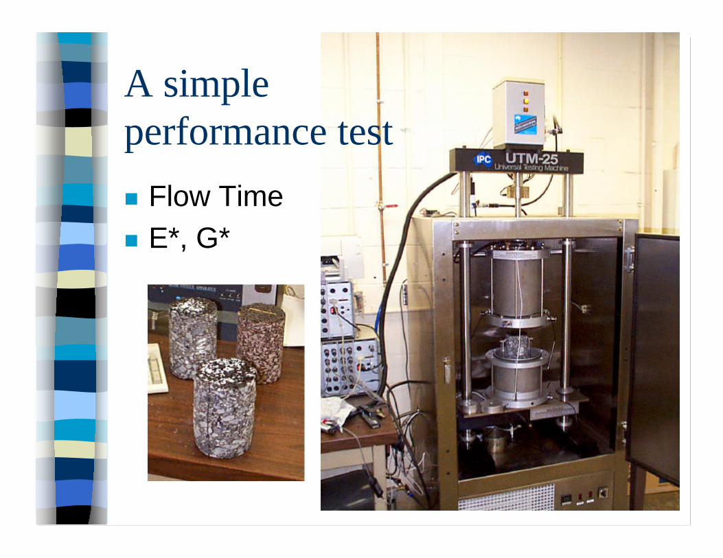
A simpleperformance test
n Flow Timen E*, G*

Selection of Materials
Performance Grade BinderMineral AggregateModifiers / Additives

Selection of Materials
n The PG binder required for the project is based on environmental data, traffic level, and traffic speed.
n The SHRP researchers developed algorithms to convert high and low air temperatures to pavement temperatures.
6

SHRP Temperature Models
n T(pav) = (T(air) - 0.00618 Lat ² + 0.2289 Lat+ 42.4) 0.9545 - 17.78– where T(pav) is the high pavement temp
at 20 mm below the surface, °C
n T(d) = T(air) + 0.051 d -0.000063 d ²– where T(d) is low pavement temp at
a depth, d, in mm, °C
6

Binder ETG & Lead States
n The original SHRP low temp algorithm do notcorrectly determine the low-pavement-temperature. The FHWA LTPP program has developed a new algorithm based on over 30 weather stations from across North America.
n The Binder ETG feels the new LTPP algorithm is far more accurate and should be used in allAASHTO documents.
6

LTPP Temperature Models
n High, T(pav)=54.32+0.78 T(air)-0.0025Lat ²-15.14 log10(H+25)+z(9+0.61F air²)½
n Low, T(pav) = -1.56+0.72 T(air)-0.004Lat² +6.26 log10(H+25)-z (4.4+0.52F air²)½
n with Reliability7

Reliability
n A factor of safety can be incorporated into the performance grading system based on temperature reliability. The 50 % reliability temperatures represent the straight average of the weather data. The 98 % reliability temperatures are determined based on the standard deviations of the low (FLow Temp ) and high (FHigh Temp ) temperature data.8

Reliability
854°
2F 3F
Average
1F
56° 58°
84
52°C
97.5 99.950%
Hot Mix, USAHigh Temp, F = 2°C

Reliability
n Tmax at 98% = Tmax at 50% + 2 * FHigh Temp
n Tmin at 98% = Tmin at 50% - 2 * FLow Temp
8

PG “Grade Bumping”
n Traffic level and speed are also considered in selecting the project PG binder either through reliability or “grade bumping.” A table is provided in AASHTO MP-2 to provide guidance on grade selection.
n This table was developed by the Superpave Lead States. 9

Grade Bumping
Adjustment to Binder PG GradeTrafficESAL’s Standing Slow Standard
< 0.3 - - -
0.3 to < 3 2 1 -
3 to < 10 2 1 -
10 to < 30 2 1 -
> 30 2 1 1
10

Author’s Note
n Use either reliability or the table to address high traffic levels and slower speeds. Both methods can effectively “bump” the PG grade such that the appropriate binder is used.
n However, using them together will result in an unnecessarily stiff binder, which may cause problems during production and lay down.
10

PG grade Increments
Average 7-day Maximum PavementTemperature
46 52 58 64 70 76 ?
Average 1-day Minimum PavementTemperature
+2 -4 -10 -16 -22 -28 ?
11

Hot Mix, USAProject Location & Historical Temperature Data
n SHRP Algorithmsn High Pvmt 53.2°Cn Low Pvmt -21.0°Cn PG 58-22 at 50%n PG 58-28 at 98%
n LTPP Algorithmsn High Pvmt 50.8°Cn Low Pvmt -14.7°Cn PG 52-16 at 50%n PG 58-22 at 98%
A. Latitude is 41.1 degrees,B. 7-day ave. max. air temp. is 33.0°C with a F of 2°C, andC. 1-day ave. min. air temp. is -21.0°C with a F of 3°C.
12

PG Selection
n For Hot Mix, USA, the 50 % reliability LTPP performance grade is a PG 52-16.
n The project traffic level and speed do not require grade bumping.
n However, the traffic speed is just above the threshold for grade bumping, and
n Historically in this area pavements have shown susceptibility to low-temperature cracking.
13

PG Selection
n Such that, the agency shall require a
n PG 58-22.
13

Performance Grade (PG) BindersAASHTO MP-1
4 Construct-ability check3Pump-ability
4 Rutting check
4 Fatigue cracking check
4 Low-temp cracking check

Binder Selection, PG 58-22
Test Temperature Property
Unaged Original
Flash PointRotational ViscosityDynamic Shear
230°C min135°C
PG High Temp
SafetyPump-ability
Rutting
Aged R.T.F.O. After Construction
Mass LossDynamic Shear PG High Temp
Age SusceptibilityRutting
Aged P.A.V 5 to 7 years
Dynamic ShearCreep Stiffness, BBR
Intermediate TempPG Low Temp + 10
Fatigue CrackingLow Temp Cracking
13

Binder, PG 58-22
?nQ. Will a modified
binder be required to satisfy this PG grade?

Binder, PG 58-22 = 80 < 90
Typically, if thedifference betweenthe high and lowtemperatures is less than 90°C,modificationis not required !

Binder ETG - AASHTO MP1(*)
n The Superpave low temp binder spec has been revised using a new scheme to determine the critical thermal cracking temperature.
n The new scheme unites the rheologicalproperties obtained using the BBR and the failure properties acquired the DTT.
14

PG Binders, AASHTO MP1(*)
4 Low-temp cracking check
4 Bending Beam Rheometer4 Direct
TensionTest
NEW!
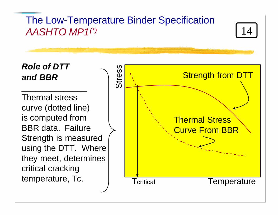
The Low-Temperature Binder SpecificationAASHTO MP1(*)
Stre
ss
Temperature
Thermal StressCurve From BBR
Strength from DTTRole of DTTand BBR______________Thermal stress curve (dotted line)is computed fromBBR data. FailureStrength is measuredusing the DTT. Wherethey meet, determinescritical cracking temperature, Tc. Tcritical
14

Reserve Strength for Lowand High m-value
Str
ess
Temperature
Low m
High m
StrengthRole of S andm-value…...______________
Binder with low m-value hasless reserve strength than high m-valuebinder and thus has less resistance to thermal fatigue.
ReserveStrength
14

Binder tests required for design
n Rotational Viscosity– SHRP adopted the Asphalt Institutes guidelines
based on the temperature-viscosity relationship– Mixing Temperature: 150 to 190 centiStokes, cSt– Compaction Temperature: 250 to 310 cSt
15

Question ?
What is a centiStoke ?
15

centi - metric prefix for 1/100
Stoke - great physicist from the 18 century, so. . . a centiStoke is square centimeter per second or one hundredth of a great dead dude.
15

centiStoke is the unit of measurementfor kinematic viscosity. Gravity inducesthe flow in this viscosity measurementand the density of the material effectsthe rate of flow. centiPoiseis the unit of absolute viscositymeasure. A partial vacuum orrotational viscometer is usedwhere gravity effects are negligible.
kinematic at 135°Cabsolute at 60°C
15

Project Binder, PG 58-22
n Gb = 1.030
n Viscosity at 135EC = 364 cP = 0.364 Pa-s
n Viscosity at 160EC = 100 cP = 0.100 Pa-s
16

Question ?
AsphaltInstitute
What are the mixingand compactiontemperatures ?
16

Answer.
n First the temperature correction factors for Gb are calculated at the test temperatures:
• CF135EC = -.0006(135EC) + 1.0135 = 0.933• CF160EC = -.0006(160EC) + 1.0135 = 0.918
n Then the test results are then converted from Pascal-seconds to centiStokes.
16

Temperature-Viscosity Chart
0.3
0.32
0.34
0.36
0.38
0.4
0.42
0.44
380 400 420 440 460 480
Log of Absolute Temperature, shown in °K (273 + °C)
Log
-Log
of
Vis
cosi
ty in
cen
tiSto
kes
CompactionRangeMixingRangePG 58-22
17

Summary of Binder Mix Testing
n Mixing Temperature Range– 148°C to 152°C
n Compaction Temperature Range– 138°C to 142°C
18

Notes on Equiviscous Temperatures
n This relationship does not work for all modified asphalt binders.
n The conversion from centipoise tocentiStokes is important, however it is not required. Determining mixing and compaction temperatures usingcentipoise will only effect the results by 1 to 2EC. 18

Selection of Materials
Performance Grade BinderMineral AggregateModifiers / Additives

Superpave utilizes a completely new system for testing, specifying, and selecting asphalt binders. While no new aggregate tests were developed, current methods of selecting and specifying aggregates were refined and incorporated.
19

Aggregate Selection
n The Gsb (bulk) and Gsa (apparent ) are determined for each aggregate. The specificgravities are used in trial binder content and VMA calculations.
Stockpiles Gsb GsaCoarse
IntermediateMan. Fines
Natural Fines
2.5672.5872.5012.598
2.6802.7242.6502.673
19

Specific Gravity Tests for Aggregates
n Two tests are needed– Coarse aggregate
(retained on the 4.75 mm sieve)
– Fine aggregate(passing the 4.75 mm sieve)

Coarse AggregateSpecific Gravityn ASTM C127
– Dry aggregate– Soak in water for 24 hours– Decant water– Use pre-dampened towel to get SSD– Determine mass of SSD agg in bucket– Determine mass under water– Dry to constant mass– Determine oven dry mass
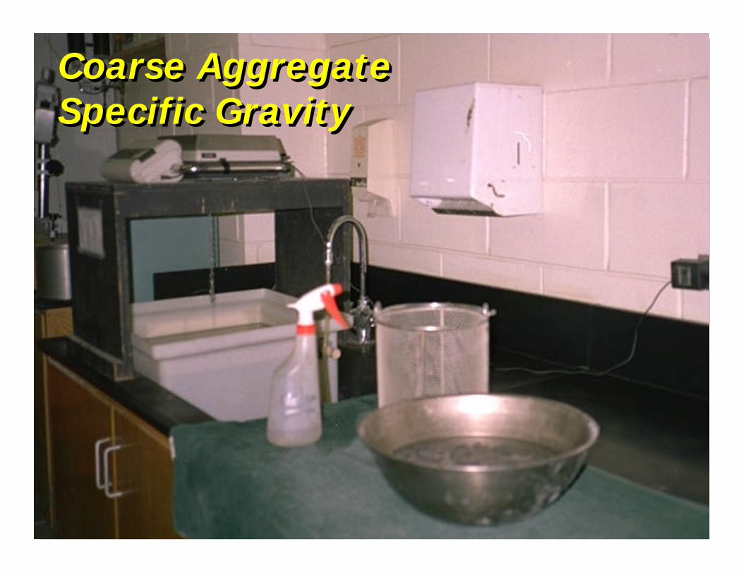
Coarse Aggregate Specific GravityCoarse Aggregate Specific Gravity

Coarse Aggregate Specific GravityCoarse Aggregate Specific Gravity

Coarse AggregateSpecific GravityCalculations
n Gsb = A / (B - C)– A = mass oven dry– B = mass SSD– C = mass under water
n Gs,SSD = B / (B - C)n Gsa = A / (A - C)n Water absorption capacity, %
– Absorption % = [(B - A) / A] * 100

Fine Aggregate Specific Gravityn ASTM C128
– Dry aggregate– Soak in water for 24 hours– Spread out and dry to SSD– Add 500 g of SSD agg to pyc of known volume
• Pre-filled with some water
– Add more water, agitate until air bubble are removed– Fill to line, determine the mass of the pycnometer,
aggregate and water– Empty aggregate into pan and dry to constant mass– Determine oven dry mass

Fine Aggregate Specific GravityFine Aggregate Specific Gravity

Fine Aggregate Specific GravityFine Aggregate Specific Gravity

Fine Aggregate Specific Gravity
Fine Aggregate Specific Gravity

Fine Aggregate Specific GravityCalculations
n Gsb = A / (B + S - C)– A = mass oven dry– B = mass of pycnometer filled with water– C = mass pycnometer, SSD agg and water– S = mass SSD aggregate
n Gs,SSD = S / (B + S - C)n Gsa = A / (B + A - C)n Water absorption capacity, %
– Absorption % = [(S - A) / A] * 100

Consensus Property Standards
n Coarse Aggregate Angularity– ASTM D 5821
n Fine Aggregate Angularity– AASHTO T 304-96
n Flat & Elongated Particles– ASTM D 4791
n Sand Equivalent– AASTHO T 176 20

Source Property Standards
n LA Abrasion– AASHTO T 96
n Soundness– AASHTO T 104
n Clay Lumps & Friable Particles– AASHTO T 112
Set by Specifying Agency (DOT)
20

Author’s Note
n An aggregate which does not individually comply with the criteria is not eliminated from the aggregate blend.
n However, its percentage of use in the total aggregate blend is limited.
20

Coarse Aggregate Angularity, CAA
n What is a fractured face?
n ASTM D5821, Percentage of FracturedParticles in Coarse Aggregates
n FRACTURED FACES - “A face will be considered a ‘fractured face’ only if it has a projected area at least as large as one quarter of the maximum projected area (maximum cross-sectional area) of the particle and the face has sharp and well defined edges.”20

Coarse Aggregate Angularity, CAA
. . .and the face has sharp and well defined edges.”

0% Crushed 100% with 2 or More Crushed Faces
Coarse Aggregate Angularity, CAA

Coarse Aggregate Angularity, CAA
Traffic Depth from Surface ESALs < 100 mm > 100 mm
. . .3 to < 10 85/80 60/ -
. . .
. . .85% one fractured face
80% two+ fractured faces
Minimum

Coarse Aggregate Angularity
n Increase Resistance to:– Rutting– Fatigue Cracking– Low-temperature Cracking
n Effect:– Production– Lay-down

Fine Aggregate Angularity
Natural sands: typically < 45
Manufactured sands: typically > 42
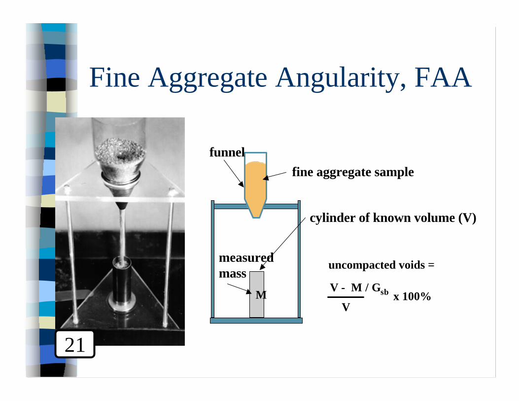
Fine Aggregate Angularity, FAA
fine aggregate sample
cylinder of known volume (V)
uncompacted voids =
V - M / Gsb
Vx 100%
funnel
M
measuredmass
21

Fine Aggregate Angularity, FAA
n Uncompacted Voids, U = (V - W / Gsb) 100V
SP
21

Fine Aggregate Angularity, FAA
n Increase Resistance to:– Rutting– Fatigue Cracking– Low-temperature Cracking
n Effect:– Production– Lay-down
21

Flat & Elongated Particles, F&E
n Superpave uses a singlemeasurement be made for flat/elongated particles.
n The 5:1 ratio refers simply to the maximum to minimum dimension.
21
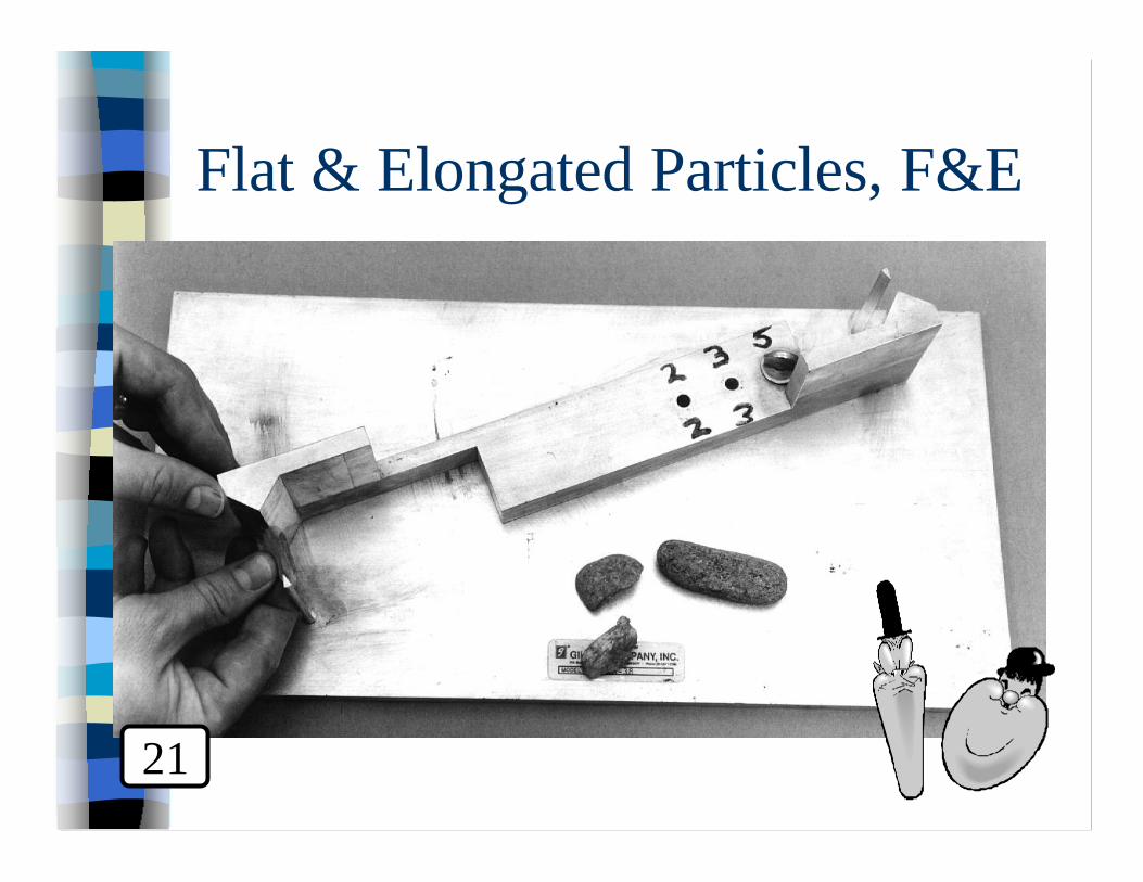
Flat & Elongated Particles, F&E
21

Flat & Elongated Particles, F&E
n Increase Resistance to:– Rutting– Fatigue Cracking– Low-temperature Cracking
n Effect:– Production– Lay-down
21

Sand Equivalent, SE
n Clay content is the percentage of clay material contained in the aggregate fraction that is finer than a 4.75 mm sieve.
n SE = 100 (SR/CR)
clay reading
sand reading
22

Bottle of Solution on Shelf Above Top of Cylinder
Hose and Irrigation Tube
Measurement Rod

Marker on Measurement Rod
Top of Suspended Material
Top of Sand Layer

Sand Equivalent, SE
n Increase Resistance to:– Rutting– Fatigue Cracking– Low-temperature Cracking
n Effect:– Production– Lay-down

Lead States
n A consolidated table has been developed for the consensus property standards criteria.
n This new table has 5 traffic levels; to correspond to the new SGC compaction criteria.
25

1999 Consensus Criteria
CAA FAAESAL
< 100 > 100 < 100 > 100SE F&E
< 0.3 55/- -/- - - 40 -0.3 to <3 75/- 50/- 40 40 403 to < 10 85/80 60/- 45 40 4510 to<30 95/90 80/75 45 40 45
> 30 100 100 45 45 50
10
25

Hot Mix, USA: CAA
nQ. Do the stockpiles meet the criteria, Y/N? If the answer is “no,” what does this mean?
(a) Stockpile can not be used, or(b) Percentage of stockpile in blend is limited.
Stockpile Results CriteriaCoarse 99 / 97 85 / 80
Intermediate 80 / 60 85 / 80
26

Stockpile Results CriterionMan. Fines 48 45
Natural Fines 42 45
Hot Mix, USA: FAA
nQ. Do the stockpiles meet the criteria, Y/N? If the answer is “no,” what does this mean?
(a) Stockpile can not be used, or(b) Percentage of stockpile in blend is limited.
26

Author’s Note
n Fine aggregates with higher fine aggregate angularity may aid in the development of higher voids in mineral aggregate (VMA).
26

Stockpile Results CriterionCoarse 9 ?
Intermediate 2
Hot Mix, USA: F&E
nQ. Do the stockpiles meet the criteria, Y/N? If the answer is “no,” what does this mean?
(a) Stockpile can not be used, or(b) Percentage of stockpile in blend is limited.
27

Stockpile Results CriterionIntermed Agg 45
Man. Fines 51 ?Natural Fines 39
Hot Mix, USA: SE
nQ. Do the stockpiles meet the criteria, Y/N? If the answer is “no,” what does this mean?(a) Stockpile can not be used, or(b) Percentage of stockpile in blend is limited.
27

Original versus 1999nQ. For this project, did any of the criteria
change from using the original tables versus the new standards in AASHTO MP-2?
27
Consensus Original Current ‘99
CAAFAAF&ESE
85 /80451045
85 /80451045

Mixture ETG Discussion
n Stockpile data collected as part of DP90 was offered for discussion of the use of the 3:1 ratio.
n 27 Stockpiles from 12 different projects sites located in:– California, Nevada, Alabama, Maine, Louisiana,
Missouri, Illinois, South Carolina, Connecticut, Texas, Wisconsin, Minnesota, and Oklahoma.
30

F&E, 5:1 versus 3:1
0
10
20
30
1 4 7
10
13
16
19
22
25
5 to 1
Stockpiles
5 to 13 to 1
30

F&E, 5:1 versus 3:1
0
20
40
60
80
100
5 10 15 20 25 30
3 to 15 to 1
Criteria (maximum)
3 to 15 to 1
Percent of Data within Criteria
30

Author’s Note
n It is recommended each specifying agency should perform a market analysis to access the impact of specifying a 3:1 source property standard.30

Source Property Standards
n LA Abrasion– Max loss approximately 35% to 40%
n Soundness– Max loss approximately 10% to 20%
n Clay Lumps & Friable Particles– Max range from 0.2% to 10%
31

Selection of a Design Aggregate Structure
FHWA 0.45 Power ChartControl Points / Restricted ZoneSuperpave Gyratory Compactor

Design Aggregate Structure
n The FHWA 0.45 Power chart is used to define permissible gradations.– Nominal Maximum Sieve Size: One
standard sieve size larger than the first sieve to retain more than 10 percent.
– Maximum Sieve Size: One standard sieve size larger than the nominal maximum size.
33

Question ?
What is a "standard" sieve ?
33

“Standard Sieves”
33
Standard Sieves, mm
50.037.525.019.012.59.54.75
2.361.180.600.300.150.075

"Joe Engineer"
What if I decide notto use the "standard"
sieves?
33

You'll design asphalt mix,but it will NOT beSuperpave !
33

The Match Game - Round 1
Ms. Metric meets Mr. English
(A) 0.15 mm(B) 0.075 mm(C) 19.0 mm
No. 200 Sieve
34

The Match Game - Round 1
Ms. Metric meets Mr. English
(A) 0.15 mm(B) 0.075 mm(C) 19.0 mm
No. 200 Sieve
34

The Match Game - Round 2
Ms. Metric meets Mr. English
(A) 9.5 mm(B) 19.0 mm(C) 12.5 mm
1/2” Sieve
34

The Match Game - Round 2
Ms. Metric meets Mr. English
(A) 9.5 mm(B) 19.0 mm(C) 12.5 mm
1/2” Sieve
34

The Match Game - Round 3
Ms. Metric meets Mr. English
(A) 4.75 mm(B) 9.5 mm(C) 2.36 mm
1/4” Sieve
34

The Match Game - Round 3
Ms. Metric meets Mr. English
(A) 4.75 mm(B) 9.5 mm(C) 2.36 mm(D) None of the above!
1/4” Sieve
34

Gradation Criteria
n Control Points– Maximum Size– Nominal Maximum Size– Key Sieves: 0.075 and 2.36 mm
n Recommended Restricted Zone– Starting from 0.30 to 2.36 or 4.75 mm
35

Gradation Criteria - 19 mm Mix
35
Sieve, mm Minimum Maximum
25.019.0
2.360.075
10090
232
100100
498
Recommended Restricted Zone
2.361.180.600.30
34.628.320.713.7
34.622.316.713.7

FHWA 0.45 Power Chart
0
20
40
60
80
100
0 0.5 1 1.5 2 2.5 3 3.5 4 4.5
Sieve Size raised to the 0.45 Power
Per
cent
Pas
sing Control
PointsRestrictedZoneMax Density
37

FHWA 0.45 Power Chart
0
20
40
60
80
100
0 0.5 1 1.5 2 2.5 3 3.5 4 4.5
Sieve Size raised to the 0.45 Power
Per
cent
Pas
sing
ControlPointsRestrictedZoneMax Density
Trial No. 1
37

FHWA 0.45 Power Chart
0
20
40
60
80
100
0 0.5 1 1.5 2 2.5 3 3.5 4 4.5
Sieve Size raised to the 0.45 Power
Per
cent
Pas
sing
ControlPointsRestrictedZoneMax Density
Trial No. 1Trial No. 2
37

FHWA 0.45 Power Chart
0
20
40
60
80
100
0 0.5 1 1.5 2 2.5 3 3.5 4 4.5
Sieve Size raised to the 0.45 Power
Per
cent
Pas
sing
ControlPointsRestrictedZoneMax Density
Trial No. 1Trial No. 2Trial No. 3
37

Estimated Trial Blend PropertiesHuber’s Method
38
n Determine what portion of the stockpiles apply to consensus property standard for each trial blend.
n Example: CAA for 1 fractured face forTrial Blend No. 1

Estimated Trial Blend PropertiesHuber’s Method
38
Stockpile CAA(A)
TrialBlend #1
(B)% of
+4.75mm
(AxB)% Appto CAA
Coarse 99/97 46 % 97 % 44.6 %
Inter. 80/60 24 % 75 % 18 %
Man.Fines
/ 15 % 0 % 0
NaturalFines
/ 15 % 0 % 0
Portion of the stockpiles that apply to consensus property.

Huber’s Method
n C = Test result, andn D = Portion of the stockpile that applies
to consensus property standard,n n = Stockpile number.
Est. Property = [(CxD)1 +(CxD)2… n][(D)1 + (D)2 … n]
38

Estimated Trial Blend PropertiesHuber’s Method
38
Stockpile(C)
CAA+1
(D)% Appto CAA
(CxD)
Coarse 99 44.6 % 44.2 %
Inter. 80 18 % 14.4 %
n Est. Property = [(CxD)1 +(CxD)2… n][(D)1 + (D)2 … n]

Estimated Trial Blend PropertiesHuber’s Method
38
Stockpile(C)
CAA+1
(D)% Appto CAA
(CxD)
Coarse 99 44.6 % 44.2 %
Inter. 80 18 % 14.4 %
n CAA +1 = [(99x44.2) +(80x14.4)][(44.2) + (14.4)]

Estimated Trial Blend PropertiesHuber’s Method
38
Stockpile(C)
CAA+1
(D)% Appto CAA
(CxD)
Coarse 99 44.6 % 44.2 %
Inter. 80 18 % 14.4 %
n CAA +1 = [(4375.8) +(1152)] = 94 %[(58.6)]

Estimating Trial Blend Properties
Q. What is CAA 2+ and SE forTrial Blend No.3 ?
39

Answers.
n CAA 2+ = 81n SE = 44.47 = 44
40

What’s Next ?
n Based upon project environment and traffic we have selected a PG binder, PG 58-22.
n Based upon traffic and layer location we have set consensus criteria and accessed our stockpiles.
n Using the FHWA 0.45 power chart we have developed trial blends. . .
40

Next we need to. . .
n Estimated asphalt binder contents for the trial blends,
n Mix and compact the trial blends in the Superpave gyratory compactor (SGC),
n Evaluate the trial blends volumetrically, and
n Select the Design Aggregate Structure.
40

Goals of Compaction
n Simulate field densification–traffic–climate
n Accommodate large aggregatesn Measure compact-abilityn Conducive to QC

Superpave Gyratory Compactor
n Basis–Texas equipment–French operational
characteristicsn 150 mm diameter
–up to 37.5 mm nominal sizen Height Recordation
??
????

Superpave Gyratory Compactor
150 mm diameter mold
ram pressure600 kPa
1.25 degrees30 gyrationsper minute

FHWA Pooled Fund PurchaseSuperpave Gyratory Compactor

Estimating Trial Binder Contents
n Based on experience for a 19.0 mm nominal, surface mix, the asphalt binder content should be. . ?
40

The Calculations
n Step 1: Estimate Gsen Step 2: Estimate Vban Step 3: Estimate Vben Step 4: Estimate Pbi, (binder - initial)
"by computer""by hand"40
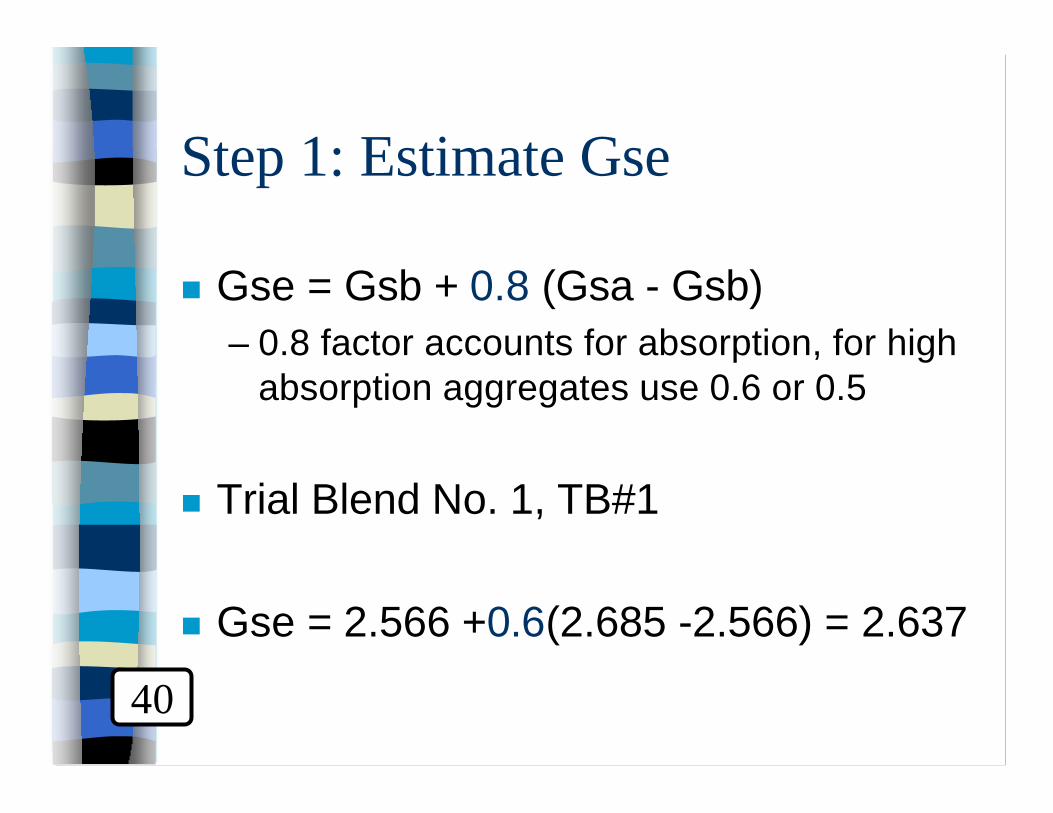
Step 1: Estimate Gse
n Gse = Gsb + 0.8 (Gsa - Gsb)– 0.8 factor accounts for absorption, for high
absorption aggregates use 0.6 or 0.5
n Trial Blend No. 1, TB#1
n Gse = 2.566 +0.6(2.685 -2.566) = 2.637
40

Step 2: Estimate Vba
n Vba = f(Va, Pb, Ps, Gb, Gsb, Gse)
– Va = 0.04, 4% voids– Pb = 0.05, (approximately 5% binder)– Ps = 1 - Pb = 0.95
n TB#1: Vba = 0.0233
41

Step 3: Estimate Vbe
n Vbe = 0.176 - 0.0675 Ln (Sn)– Sn = Nominal maximum size in mm
n Vbe = 0.176 - 0.0675 Ln(19) = 0.090– This value is true for all blends.
41

Step 4: Estimate Pbi
n Pbi = f(Va, Gb, Gse, Vbe, Vba)
n TB#1: Pbi = 4.95 %
n Author’s Note: The equations can not replace experience.
42

Summary of Estimated Pbi
Trial Blend Pbi Use123
4.954.984.95
5.05.05.0
42

Required Testing
Trial Blend SGC Rice, Gmm123
3 (4800 g/ea)33
2 (2000 g/ea)22
Total 55.2 kg 43.2 kg 12.0 kg
"the lab"43

Required Aging
n Original Specification:– Aging of both gyratory and Gmm samples,– 4 hours at 135°C in a forced-draft oven,– Mixing samples every hour.
44

Required Aging ‘99
n Specimens are mixed at the equiviscous mixing temperature.
n Specimens are short term aged for 2-hours at the equiviscous compaction temperature in a forced-draft oven.
n This is only for volumetric design.
45

Aging

History Lesson on Compaction
n SHRP researcher evaluated 9 GPS sites to develop the original SGC compaction table.
n Mixture ETG conducted the “N-design II” study using data for State projects, TFHRC, and WesTrack.
n NCHRP 9-9 investigated the sensitivity of the original compaction table
46

History continued. . .
n September 23, 1998, a date which changed SGC compaction forever.– Mixture ETG, Baltimore, Maryland
46

Compaction

SGC Criteria
n N ini - “Tenderness Check”represents the mix during construction. Mixes that compact too quickly in the SGC may have tenderness problems during construction.
n N des - . . .n N max - . . .
58

SGC Criteria
n N inin N des - “Volumetric Check”
Represents the mix after construction and initial trafficking. Mix volumetrics, (Va, VMA, and VFA), are compared to empirically based criteria.
n N max - . . .
58

SGC Criteria
n N inin N desn N max - Optional “Rutting Check”
Mixes that commonly rut have been compacted below 2% air voids under traffic. Mixes compacting below 2% air voids in the SGC may have rutting problems.
58

Why Volumetrics ?Colorado Study
0
1
2
3
4
5
6
7
8
0 5 10 15 20 25 30 35
Projects (Sorted by Air Voids)
In-p
lace
Air
Voi
ds (
Whe
el P
ath)
RuttingNo Ruts3% Va

Original SGC Compaction Effort
EstimatedTraffic
< 39°C 39°-40°C 41°-42°C 43°-44°C
< 0.3< 1< 3
< 10< 30
< 100> 100
68
172
7 Day Average Design High Air Temperature
28Compaction
Levels

SGC Compaction Effort ‘99ESAL’s N ini N des N max App
< 0.3 6 50 75 Light
0.3 to < 3 7 75 115 Medium
3 to < 30 8 100* 160 High
10 to <30 8 100 160 High
> 30 9 125 205 Heavy
47
Base mix (< 100 mm) option to drop one level, unless the mix will be exposed to traffic during construction.

Q. What shouldVMA criteria bea function of ?

Voids in Mineral Aggregate, VMA
10
11
12
13
14
15
16
0 5 10 15 20 25 30 35 40
Nominial Maximum Sieve Size, mm
Min
imum
VM
A

Volumetric Design Criteria ‘99
SGC CriteriaTrafficESAL Nini Ndes Nmax
VMA VFA FinesPbe
< 0.3 <91.5 70-80< 3 <90.5 65-78
< 10 <89.0< 30 <89.0> 30 <89.0
=96.0 <98.0 n/a65-75
0.6 -to-1.2
49

Property CriteriaNini / %Gmm
Ndes / %Gmm
Nmax / %Gmm
VMAVFA
Dust-to-Binder
Hot Mix, USA
Est. 20-year design traffic is 6.3M ESAL’s
52

Hot Mix, USA
Property CriteriaNini / %Gmm
Ndes / %Gmm
Nmax / %Gmm
VMAVFA
Dust-to-Binder
8 gyr < 89%100 gyr = 96%160 gyr < 98%
13.0 min65 to 750.6 to 1.2
52
Est. 20-year design traffic is 6.3M ESAL’s

SGC Compaction Curve
n % Gmm vs Log (No. of Gyrations)– Height is monitored during compaction and
is used to calculate the densification of the specimen, expressed as % Gmm.
%Gmm des = Gmb * 100Gmm
52
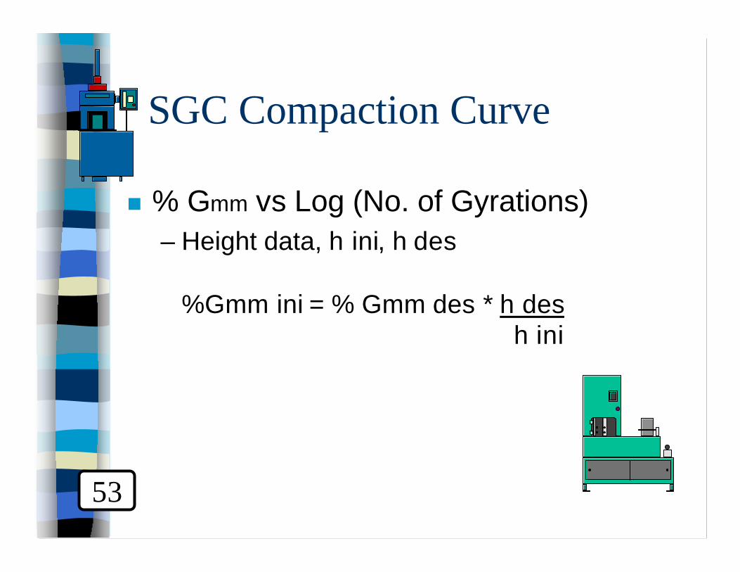
SGC Compaction Curve
n % Gmm vs Log (No. of Gyrations)– Height data, h ini, h des
%Gmm ini = % Gmm des * h desh ini
53

SGC Compaction Calculations
n Trail Blend No. 1
n Gmm = 2.475– Specimen 1, Gmb = 2.351– Specimen 1, Gmb = 2.348– Specimen 1, Gmb = 2.353
54

SGC Calc’s for Trial Blend No. 1
n Specimen 1
n %Gmm des = Gmb * 100 = 2.351 * 100Gmm 2.475
n %Gmm des = 95.0 % = 96.0% Criterion
55

SGC Calc’s for Trial Blend No. 1
n Q. What are they for specimens 2 & 3 ?
n %Gmm des = Gmb * 100 = ? Gmm
55

SGC Calc’s for Trial Blend No. 1
n %Gmm max for specimens 2 & 3:
n 2, %Gmm des = 94.9 %n 3, %Gmm des = 95.1 %
55

SGC Height Data
n Trail Blend No. 1
n %Gmm ini = 95.0*(117.4/129.6) = 86.1%55
TB 1Specimen H ini H des
% Gmm
at N des
123
129.6129.8129.9
117.4117.4117.8
95.0 %94.9 %95.1%

%Gmm ini
55
What is %Gmm inifor specimens 2 & 3 ?

%Gmm ini
n 2: %Gmm ini = 85.8 %
n 3: %Gmm ini = 86.2 %
56

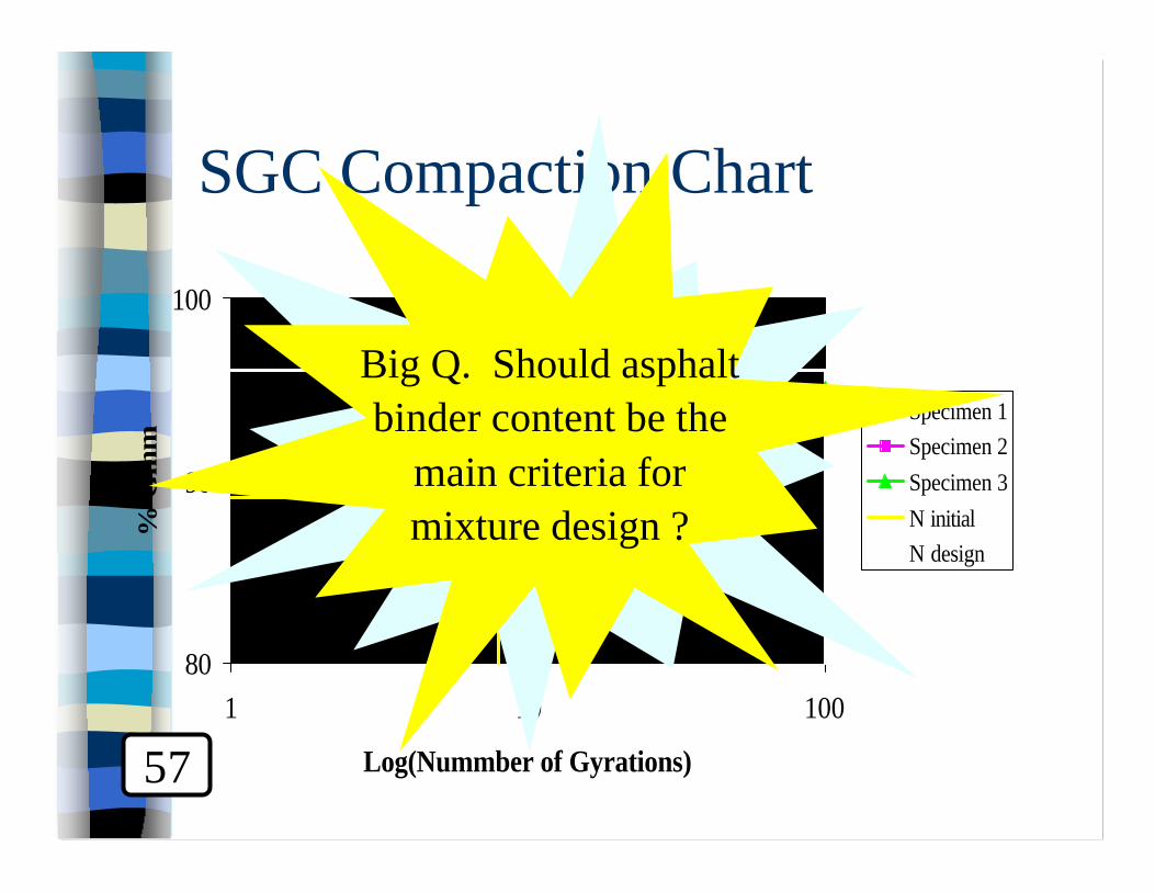
SGC Compaction Chart
80
90
100
1 10 100
Log(Nummber of Gyrations)
% G
mm
Specimen 1Specimen 2Specimen 3N initialN design
57

SGC Compaction Chart
80
90
100
1 10 100
Log(Nummber of Gyrations)
% G
mm
Specimen 1Specimen 2Specimen 3N initialN design
57

SGC Compaction Chart
80
90
100
1 10 100
Log(Nummber of Gyrations)
% G
mm
Specimen 1Specimen 2Specimen 3N initialN design
57

Q. Is binder content high or low?
80
90
100
1 10 100
Log(Nummber of Gyrations)
% G
mm
Specimen 1Specimen 2Specimen 3N initialN design
57
SGC Compaction Chart
80
90
100
1 10 100
Log(Nummber of Gyrations)
% G
mm
Specimen 1Specimen 2Specimen 3N initialN design
57
Big Q. Should asphaltbinder content be the
main criteria formixture design ?

Trial Blends
80
90
100
1 10 100
Log(Nummber of Gyrations)
% G
mm
Trial Blend 1Trial Blend 2Trial Blend 3N initialN design
59

How do we choose ?
We need to adjust theresults to reflect 4.0 %
voids at N des ?
60

Trial Blend No. 1
80
90
100
1 10 100
Log(Nummber of Gyrations)
% G
mm Trial Blend 1
AdjustedN initialN design

Trial Blend No. 2
80
90
100
1 10 100
Log(Nummber of Gyrations)
% G
mm Trial Blend 2
N initialN design

Trial Blend No. 3
80
90
100
1 10 100
Log(Nummber of Gyrations)
% G
mm Adjusted
Trial Blend 3N initialN design

Estimating the Properties at 4% Va
n 1) Estimate binder contentn 2) Estimate VMAn 3) Estimate VFAn 4) Estimate %Gmm inin 5) Estimate Dust-to-Binder ratio
60

Estimate Pb with 4% Va
n Pb, est = Pbi - [0.4 *(4 - Va at N des)]
n Rule: 1 % Air Voids = 0.4 % Binder
60

Estimate VMA at Ndes w/ 4% Va
n VMA, est = VMA + C (4 - Va at N des)
– C = constant (either 0.1 or 0.2)– C = 0.1, when Va is less than 4.0%– C = 0.2, when Va is 4.0% or greater
60

Estimate VFA at Ndes w/ 4% Va
n VFA, est = 100 (VMA, est - 4)VMA, est
60

Estimate %Gmm ini & %Gmm max
n %Gmm ini, est = %Gmm ini -(4 - Va at N des)
60
Trial Blend No. 1
80
90
100
1 10 100
Log(Nummber of Gyrations)
% G
mm Trial Blend 1
AdjustedN initialN design

Estimate F/Pbe w/ 4% Va
n Pbe, est = f(Gb, Gse, Gsb, Pb est)
n Author’s Note: The Dust-to-Binder ratio in Superpave is based upon the effective asphalt binder content, NOT the total.
61

Property CriteriaN ini / % Gmm
N des / % Gmm
VMAVFA
Dust-to-Binder
8 gyr < 89%100 gyr = 96%
13.0 min65 to 750.6 to 1.2
Compare Estimated Propertiesto Volumetric Criteria
SP
61

TrialBlends Pb
VMAat Ndes
VFA atNdes
FinesPbe
%Gmm
at Nini
123
5.45.05.2
13.813.013.4
716970
0.820.811.15
87.186.590.1
Criteria - 13 min 65-75 0.6-1.2 89 max
Summary of Estimated Properties
Is everythingokay ?
61

TrialBlends Pb
VMAat Ndes
VFA atNdes
FinesPbe
%Gmm
at Nini
123
5.45.05.2
13.813.013.4
716970
0.820.811.15
87.186.590.1
Criteria - 13 min 65-75 0.6-1.2 89 max
Summary of Estimated Properties
Is everythingokay ?
61

Design Aggregate Structure
0
20
40
60
80
100
0 0.5 1 1.5 2 2.5 3 3.5 4 4.5
Sieve Size raised to the 0.45 Power
Per
cent
Pas
sing
ControlPointsRestrictedZoneMax Density
Trial No. 1
Trial Blend No. 1
62
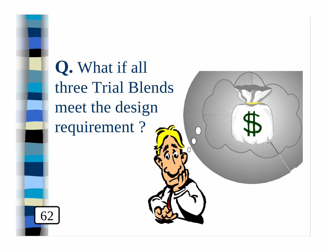
Q. What if all three Trial Blends meet the design requirement ?
62

Selection of theDesign Asphalt Binder Content
Optimum Pb

Design Asphalt Binder Content
n Specimens are compacted at varying asphalt binder contents:– Estimated asphalt binder content– + 0.5 %– + 1.0 %
Optimum63

Lead States
n Based upon the recommendations of NCHRP 9-9,
n Optimization of the design aggregate blend is only compacted to Ndes
n Check the design aggregate blend at the optimum asphalt compacted to Nmax.63

Required Tests
BatchedPb
SGCSpecimens
GmmRice
4.9 (- ½ %)5.4 (Target)5.9 (+ ½ %)6.4 (+ 1 %)
3 (4800 g/ea)333
2 (2000 g/ea)222
Total 57,600 g 16,000 g
63

SGC Compaction Chart
80
90
100
1 10 100
Log(Nummber of Gyrations)
% G
mm
6.40%5.90%5.40%4.90%N initialN design
64

Summary of Optimization
Property Results CriteriaVa at Ndes
VMA at Ndes
VFA at Ndes
F / Pbe ratio%Gmm ini
%Gmm max
4.013.570
0.8786.9n/a
4.013.0 min65 to 75
0.6 to 1.2< 89< 98
65

Summary of Optimization
1.0
2.0
3.0
4.0
5.0
6.0
4.5 5.5 6.5
Va
at N
des
60.0
65.0
70.0
75.0
80.0
85.0
90.0
4.5 5.5 6.5
Asphalt Binder Content
VFA
at N
des
0.4
0.6
0.8
1.0
1.2
1.4
Asphalt Binder Content
DU
ST-T
O-B
IND
ER
10.0
11.0
12.0
13.0
14.0
15.0
16.0
4.5 5.5 6.5
VM
A a
t Nde
s
Va VMA
VFA F/Pbe
66

Design Blend at OptimumRutting Check
80
90
100
1 10 100 1000
Log(Nummber of Gyrations)
% G
mm Optimum AC
N initialN designN maximum

Author’s Note
n If you have limited experience with the trial gradations. It is recommended during the selection of the design aggregate structure that you compact at least one specimen to Nmax to assess the blends ability to resist rutting.

Evaluation of Moisture Sensitivity
AASHTO T-283

Evaluation of Moisture Sensitivity
Measured on Proposed Aggregate Blend and Asphalt Content
Tensile Strength Ratio
80 %minimum
3 Conditioned Specimens
3 Dry Specimens
Evaluation of Moisture Sensitivity
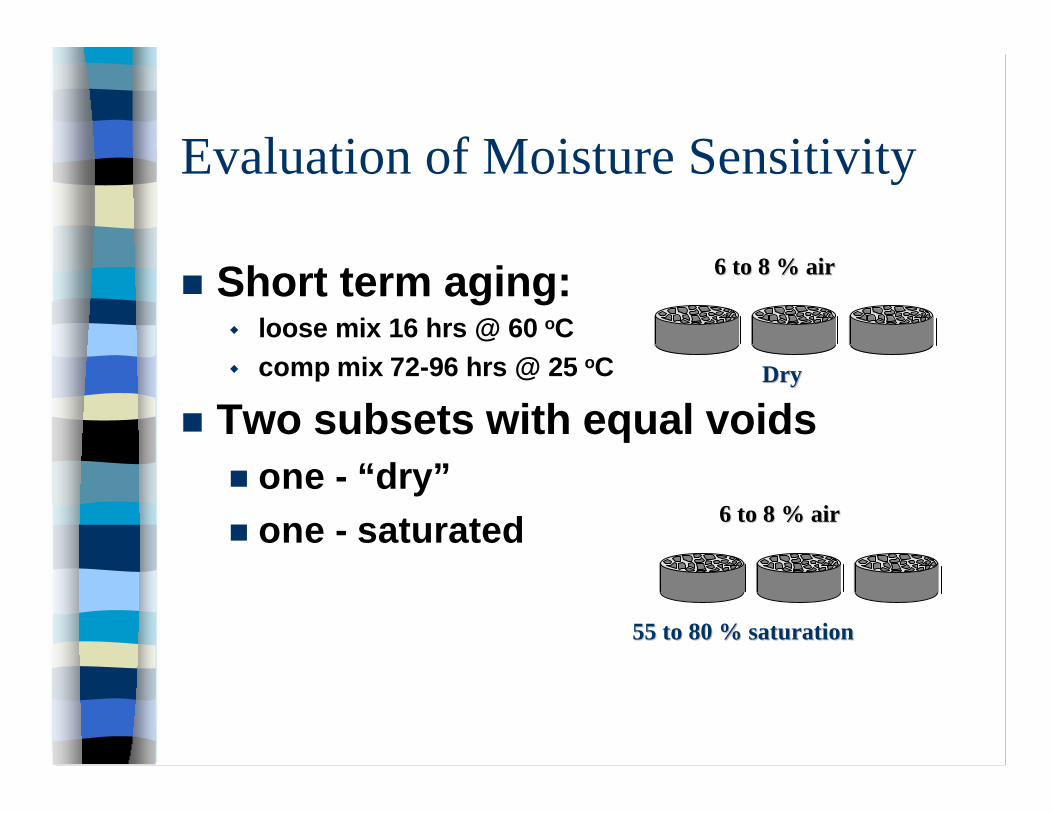
n Short term aging:w loose mix 16 hrs @ 60 oCw comp mix 72-96 hrs @ 25 oC
n Two subsets with equal voidsn one - “dry”n one - saturated
DryDry
6 to 8 % air6 to 8 % air
6 to 8 % air6 to 8 % air
55 to 80 % saturation55 to 80 % saturation

Evaluation of Moisture Sensitivity
nn optional freeze cycleoptional freeze cyclenn hot water soakhot water soak
16 hours @ -18 oC
24 hours @ 60 oC

Evaluation of Moisture Sensitivity
AvgAvg DryDry Tensile StrengthTensile Strength AvgAvg Wet Wet Tensile StrengthTensile Strength
TSR = TSR = ≥≥ 80 %80 %WetWet
DryDry
51 mm / min @ 2551 mm / min @ 25 ooCC

Evaluation of Moisture Sensitivity
AASHTO T-283Samples SGC ITS
UnconditionedDry
3 Specimens7 % Va
872 kPa
ConditionedWet
3 Specimens7 % Va
721 kPa
TSR 82.7 %Superpave
Criteria80 %min
67

Question ?
What if the TSR fails ?
67

Author’s Note
n SHRP gave us the ECS
n Superpave calls for AASHTO T-283– 4” Marshall Specimens
n NCHRP 9-13 ties T-283 + gyratory– Jon Epps (University of Nevada at Reno)

Author’s Note
n In the interim agencies are. . .– Using Modified Lottman / Root-Tunnicliff
• 150 & 100 mm SGC, 4” Marshall Specimens• 100% Saturation
– Proof Tests• Asphalt Pavement Analyzer (Georgia LWT)• Hamburg Loaded Wheel Tester
– Pull-off Test (Binder/Mastic only)

Better moisture sensitivity test
n July 28, 1999 -- NCHRP hosted“Moisture Sensitivity Focus Group”
n Outcome: NCHRP project to develop a new test for moisture sensitivity

Major Steps in Superpave
n Selection of Materials,
n Selections of a Design Aggregate Structure,
n Selection of the Design Binder Content, and
n Evaluation of Moisture Sensitivity.– Mixture/Aggregate & Binder ETG– Lead States
SP

Guidelines for the use of RAP
n FHWA Mix ETG developed guidelines based upon consensus and limited testing (<15%, 15-25, 25%+).
n NCHRP 9-12, “Incorporation of RAPin the Superpave System”– Rebecca McDaniel (NC Superpave Center)

Superpave Field Management
PRODUCTION
ACCEPTANCE
PERFORMANCE
DESIGN
QC

Click here to type page title
Thank you.


FHWA 0.45 Power Chart
0
20
40
60
80
100
0 0.5 1 1.5 2 2.5 3 3.5 4 4.5
Sieve Size raised to the 0.45 Power
Per
cent
Pas
sing
ControlPointsRestrictedZoneMax Density
Trial No. 1Trial No. 2Trial No. 3

SGC Compaction Chart
80
90
100
1 10 100
Log(Nummber of Gyrations)
% G
mm
Specimen 1Specimen 2Specimen 3N initialN design

Trial Blends
80
90
100
1 10 100
Log(Nummber of Gyrations)
% G
mm
Trial Blend 1Trial Blend 2Trial Blend 3N initialN design

SGC Compaction Chart
80
90
100
1 10 100
Log(Nummber of Gyrations)
% G
mm
6.40%5.90%5.40%4.90%N initialN design

Summary of Optimization
1.0
2.0
3.0
4.0
5.0
6.0
4.5 5.5 6.5
Va
at N
des
60.0
65.0
70.0
75.0
80.0
85.0
90.0
4.5 5.5 6.5
Asphalt Binder Content
VFA
at N
des
0.4
0.6
0.8
1.0
1.2
1.4
Asphalt Binder Content
DU
ST-T
O-B
IND
ER
10.0
11.0
12.0
13.0
14.0
15.0
16.0
4.5 5.5 6.5
VM
A a
t Nde
s
Va VMA
VFA F/Pbe