Embed Size (px)
Citation preview

Superstructure-based Optimization of Membrane-based
Carbon Capture Systems
Miguel Zamarripa, Olukayode Ajayi, Michael Matuszewski, David C. Miller
National Energy Technology Laboratory, Pittsburgh, PA
Design and Optimization of Environmentally Sustainable Fossil Energy Systems
AIChE Annual Meeting 2017, Minneapolis, MN, USA.
November 2nd, 2017
1

Motivation: Current applications are insufficient to simultaneously
optimize multiple technologies, process configurations, and
operating conditions while minimizing the cost of electricity (COE).
Introduction
Goal: Develop a superstructure-based mathematical optimization framework.
Simultaneously optimize the process configuration, process design
and operating conditions based on rigorous models.
Post Combustion CO2 Capture Technologies
Solid Sorbents –adsorption
Liquid Solvents -absorption
Membranes – gas permeation
Membrane materials
• Selectivity
• permeability
Flue gas (F, T, P, x)
Systems Engineering Analysis
• COE
• Capture rate
2

Introduction
Membrane materials
• Selectivity
• permeability
Flue gas (F, T, P, x)
Systems Engineering Analysis
• COE
• Capture rate
2
Exploit the model
flexibility
• New targets
• New materials
Post Combustion CO2 Capture Technologies
Solid Sorbents –adsorption
Liquid Solvents -absorption
Membranes – gas permeation
Motivation: Current applications are insufficient to simultaneously
optimize multiple technologies, process configurations, and
operating conditions while minimizing the cost of electricity (COE).
Goal: Develop a superstructure-based mathematical optimization framework.
Simultaneously optimize the process configuration, process design
and operating conditions based on rigorous models.

Advanced process configurations
• Rigorous models.
• Fixed process configurations (simulation-optimization
frameworks).
(Merkel et al., 2010; Morinelly & Miller 2011 & 2012).
Membrane systems optimization
Superstructure based optimization
• First principles + simplified models.
• Studies focus on multi-stage configurations.
• The number of process configurations analyzed by the
optimizer is limited. (Hasan et al., 2012 and Arias et al.,
2016)
3
M1 M2 Mi3
M4 M5 M6
CO2 to
Storage
To Stack
Flue Gas

Advanced Process Configurations
Coal Power Plant
650 MW
CO2 to
Storage
T = -30 C
P = 22 bar
Multi-stage
Membrane systemCompressors
Pumps
Expanders
Membranes
Liquefier Column
To StackAir Sweep (enriched with CO2)
Compression train
– with intercooling
Boiler
Bag House
FGD
Steam Cycle
Power Plant
Flue Gas
Primary and
Secondary Air Air Sweep
Gas stream
Liquid stream
4
Systems Engineering Challenges
Large amount of gas
Low CO2 concentration
Several “potential” process
configurations

• Discrete Decisions:
• Continuous decisions:
Superstructure Optimization Framework
Permeate M1
Flue Gas Permeate M2 + sweep air
RetentateRetentate M1
CO2 to
Storage
Permeate
T = -30 C
P = 22 bar
Compressor train Mi
M2
Liquefier
Expander
Retentate M2
M1
To Stack
Air Sweep
Compression train – with
intercooling
Power Plant
How many units? NLP – bypassing the units not installed
Unit design, Operating conditions (temp, pressure, flow rates, compositions)
Expander
Mi+1Mi+2
Mi+3 Mi+4 Mi+5
Retentate
Permeate
Retentate
5

Cost of Electricity
6
𝒔. 𝒕.
Quality Guidelines for Energy System Studies:
Performing a Techno-economic Analysis for Power
Generation Plants (DOE/NETL-2015/1726)
𝑀𝑎𝑡𝑒𝑟𝑖𝑎𝑙 𝐵𝑎𝑙𝑎𝑛𝑐𝑒𝑠
𝐸𝑛𝑒𝑟𝑔𝑦 𝐵𝑎𝑙𝑎𝑛𝑐𝑒𝑠
𝐸𝑞𝑢𝑖𝑝𝑚𝑒𝑛𝑡 𝐷𝑒𝑠𝑖𝑔𝑛
min𝐶𝑂𝐸 =𝐼𝑛𝑣𝑒𝑠𝑡𝑚𝑒𝑛𝑡 + 𝑂𝑝𝑒𝑟𝑎𝑡𝑖𝑛𝑔𝑓𝑖𝑥 + 𝑂𝑝𝑒𝑟𝑎𝑡𝑖𝑛𝑔𝑣𝑎𝑟
𝑁𝑒𝑡 𝑃𝑜𝑤𝑒𝑟
𝑃𝑟𝑜𝑐𝑒𝑠𝑠 𝐶𝑜𝑛𝑓𝑖𝑔𝑢𝑟𝑎𝑡𝑖𝑜𝑛
Costing Methodology:
• Investment cost
– Power Plant, Capture
(Membrane, HX, compressor)
• Operating cost:
– Fixed: labor, maintenance, others
– Variable: utilities “coolant &
steam”, waste water, others
• Net power:
– Power PP – (kW for compression,
blowers, pumps, etc.)
𝐶𝑎𝑝𝑡𝑢𝑟𝑒 𝑇𝑎𝑟𝑔𝑒𝑡
Product and Process Design Principles Synthesis
(Seider et al., 2009)
Purchase cost calculations

• Separation stage
Single Stage
Units in stage:
- Compression system
- Heat exchanger
- Membrane
- Vacuum pump
- Expander
Flue Gas
- 10-15 % CO2
- 1 bar
- 327 K
Flue Gas
- 1-6 bar
- 350-600 K
Flue Gas
- 1-6 bar
- 298.15 K = Tmem = 298-350 K
Retentate
- 3-6 bar
- 298.15 K
Permeate
- 0.2 - 1 bar
- 298.15 K
- 0.25 – 0.8 % CO2
Permeate
- 1 bar
- 298.15 K
Compressor duty (Hp):
𝑾𝒋=𝟏,𝒔 =𝟏
𝜼
𝒊
𝑭𝑭𝒊,𝒔𝟖𝟑𝟏𝟒
𝟕𝟒𝟓. 𝟑𝑻𝒇𝜸
𝜸 − 𝟏
𝑷𝟏,𝒔𝑷𝒇
𝜸−𝟏𝜸
− 𝟏
𝑷𝟏,𝒔
𝑷𝒇𝑻𝒇
𝑾𝒋,𝒔
𝑭𝑭𝒊,𝒔
7

• Separation stage
Single Stage
Units in stage:
- Compression system
- Heat exchanger
- Membrane
- Vacuum pump
- Expander
Flue Gas
- 10-15 % CO2
- 1 bar
- 327 K
Flue Gas
- 1-6 bar
- 350-600 K
Flue Gas
- 1-6 bar
- 298.15 K = Tmem = 298-350 K
Retentate
- 3-6 bar
- 298.15 K
Permeate
- 0.2 - 1 bar
- 298.15 K
- 0.25 – 0.8 % CO2
Permeate
- 1 bar
- 298.15 K
Outlet Temperature (after compression) (K):
𝑻𝒐𝒖𝒕,𝒔 = 𝑻𝒇𝑷𝟏,𝒔𝑷𝒇
𝜸−𝟏𝜸
𝑷𝟏,𝒔
𝑷𝒇𝑻𝒇
𝑻𝒐𝒖𝒕,𝒔
7

• Separation stage
Single Stage
Units in stage:
- Compression system
- Heat exchanger
- Membrane
- Vacuum pump
- Expander
Flue Gas
- 10-15 % CO2
- 1 bar
- 327 K
Flue Gas
- 1-6 bar
- 350-600 K
Flue Gas
- 1-6 bar
- 298.15 K = Tmem = 298-350 K
Retentate
- 3-6 bar
- 298.15 K
Permeate
- 0.2 - 1 bar
- 298.15 K
- 0.25 – 0.8 % CO2
Permeate
- 1 bar
- 298.15 K
Heat exchanger duty (kW):
𝑾𝒋=𝟐,𝒔 =
𝒊
𝑭𝑭𝒊,𝒔 𝑪𝒑 𝑻𝒐𝒖𝒕,𝒔 − 𝑻𝒎𝒆𝒎
𝑾𝒋=𝟐,𝒔
𝑻𝒐𝒖𝒕,𝒔
7

• Separation stage
Single Stage
Units in stage:
- Compression system
- Heat exchanger
- Membrane
- Vacuum pump
- Expander
Flue Gas
- 10-15 % CO2
- 1 bar
- 327 K
Flue Gas
- 1-6 bar
- 350-600 K
Flue Gas
- 1-6 bar
- 298.15 K = Tmem = 298.15 K
Retentate
- 3-6 bar
- 298.15 K
Permeate
- 0.2 - 1 bar
- 298.15 K
- 0.25 – 0.8 % CO2
Permeate
- 1 bar
- 298.15 K
Vacuum pump (Hp):
𝑾𝒋=𝟑,𝒔 =𝟏
𝜼
𝒊
𝑭𝑭𝒊,𝒔𝟖𝟑𝟏𝟒
𝟕𝟒𝟓. 𝟑𝑻𝒎𝒆𝒎
𝜸
𝜸 − 𝟏
𝑷𝒂𝒕𝒎𝑷𝟐,𝒔
𝜸−𝟏𝜸
− 𝟏
𝑷𝟏,𝒔
𝑷𝟐,𝒔
𝑾𝒋,𝒔
𝑭𝑭𝒊,𝒔
7

Membrane model
Feedi
n=Nc
Retentatei
Permeatei
Retentate
Side
Permeate
Side
𝑱𝐢,𝒏 = 2𝜋𝑟𝐹𝑜𝑛𝐹𝑃
𝛿𝑃1𝑥𝑟𝑖,𝑛 − 𝑃2𝑥𝑝𝑖,𝑛
Membrane Area
(section) Permeance
(kgmol/m2 s bar)
Driving force
(partial pressure difference)
Juan Morinelli, Kayode Ayaji, CCSI toolset
Counter current flow
FPNc,s
FP0,s
𝟎 = 𝑭𝒛𝒊|𝒙 − 𝑭𝒛𝒊|𝒙+𝟏 + 𝑱𝒊|𝒙
𝟎 = −𝝏
𝝏𝒙𝑭𝒄𝒊 − 𝑱𝒊
𝝏(𝑭𝒊,𝒏 − 𝑭𝒊,𝒏−𝟏)
𝒉= −𝑱𝒊,𝒏
𝒉 =𝑳
𝑵𝒄 − 𝟏
Approximation:
8
Ji,n
Material Balances:
Main Assumptions:
• Counter current flow
• Finite differences method
• Sweep (possible)
Membrane model
FRi,n,s = FRi,n−1,s − Ji,n,s ℎ ∀𝑖, 𝑛 > 1, 𝑠
FPi,n,s = F𝑃i,n−1,s − Ji,n,s ℎ ∀𝑖, 𝑛 < Nc , 𝑠
FPi,n-1,s
FRi,n-1,s
Feedi
n=1 n=2 n=n-1 n=n n=n+1 n=Nc
Retentate
Permeate
Retentate
Side
Permeate
Side
Ji,n,s
h =L
Nc − 1
8
Sweep

• Retentate side
– Linear regression
• Permeate side
– Rigorous model (Morinelly et al., 2012)
Membrane Pressure Drop
0
0.02
0.04
0.06
0.08
0.1
0.12
0.14
0.16
0 5 10 15 20
Membrane slot
Permeate Pressure, Bars
𝑷𝒑𝒆𝒓𝝏𝑷𝒑𝒆𝒓
𝝏𝒙=𝟏𝟔𝑹𝑻𝝁𝑭𝒑𝒆𝒓
𝝅𝒓𝑭𝑰𝟒 𝒏𝑭
𝑽𝒓𝒆𝒕 =𝑭𝒓𝒆𝒕
𝑺𝑨 𝝆 𝟑𝟔𝟎𝟎
𝑺𝑨 =𝟑. 𝟏𝟒𝟐
𝟒𝒅𝒔𝟐 − 𝒏𝑭𝒅𝒇𝒐
𝟐
𝒅𝒔𝟐 =𝒏𝑭𝒅𝒇𝒐
𝟐
𝝋
𝝆 =𝒏
𝑽=𝑷
𝑹𝑻=
𝒃𝒂𝒓
𝒃𝒂𝒓.𝒎𝟑𝒌𝒎𝒐𝒍.𝑲
𝑲=𝒌𝒎𝒐𝒍
𝒎𝟑
Surrogate model:
Vapor viscosity (𝝁 – cP) (3.6e11 cP = 1 bar*hr)
𝝁*3.6e11 = 𝝁CP
Input variables: F(x {molar fractions, T, P, F})
ACM (non-ideal calculations)
R2 = 0.9990.014
0.0145
0.015
0.0155
0.016
0.0165
0.014 0.0145 0.015 0.0155 0.016 0.0165
Pre
dic
ted (
surr
ogate
)
Rigorous (ACM)
𝝁 Permeate in CP
9

Case study (test example + model comparison)
Case study
• 650 MW power plant
• 90% Capture
• 99% CO2 pure to storage
• 3 - 6 membranes
• α CO2/(Ar, O2, N2)=100
• α CO2/H2O=0.5
• Permeance = 0.1204
(kgmol/m2 s bar)
Model Simulation (ACM) Optimization (GAMS)
Compressor Centrifugal compressor Polytropic compressor
Flash calc. Non-ideal Ideal calculations
Liquefier Non-ideal flash Surrogate model
10
Pe
rme
ate
M1
Flue Gas Permeate M2 + sweep air
RetentateRetentate M1
CO2 to
Storage
Permeate
T = -30 C
P = 22 bar
Compressor train M3
M2
Liquefier
Expander
Retentate M2
M1
To Stack
Air Sweep
Compression train – with
intercooling
Boiler
Expander
M4
M5 M6
Retentate Mi
Permeate
Retentate
Test example
- ACM Simulation (CCSI toolset)
Power Plant

Liquefier (flash tank)
Flash Formulation
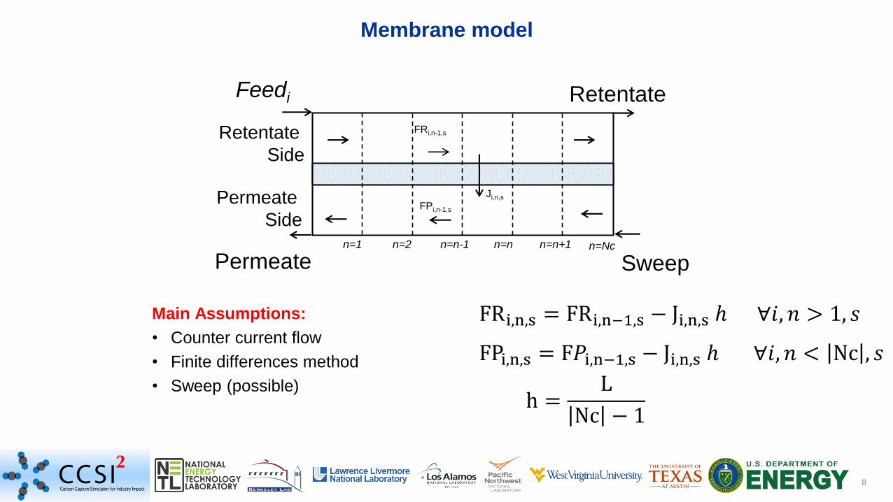
Flash Model (flash tank):
Non-Ideal calculations are replaced by a surrogate model
Operating Conditions:
Flue gas temp: 25-50 C
Flue gas pressure: 15-30 bars
Flue gas molar fractions (CO2): 0.5-0.89 kmol/kmol
TFL: -40 to -20 C
Surrogate models for Gas outlet (ALAMO):
r2(FG) = 0.978, r2(FCO2) = 0.992, r2(FN2 FO2 FAr) = 0.999
T = -30 C
P = 22 bar
Flow= X
T = 38 C
P = 22 bar
CO2 = 0.8-0.92
Variables:
Flue Gas: FF, TF, PF, XFi
Gas: FG, TG, PG, yi
Liquid: FL, TL, PL, xLi
Flash Tank: TFL, PFL, QFL
27 variables (i = 5)
FF, TF, PF, XFi
FG, TG, PG, yi
FL, TL, PL, xL
i
TFL, PFL
Equations:
PF = PFL = PL = PG
TFL = TG =TL
FG = f(FF, TF, PF, xFi, TFL)
Fyi = f(FF, TF, PF, xFi, TFL)
QFL = f(FF, TF, PF, xFi, TFL)
FL = FF – FG
xLi = (xF
i FF – Fyi)/FL
18 equations
Degrees of Freedom: 27 – 18 = 9 (8 Feed + TFL)
# Eqns:
3
2
1
5
1
1
5
18 eqnsOptimization Variables
11
Case study (test example + model comparison)
Case study
• 650 MW power plant
• 90% Capture
• 99% CO2 pure to storage
• 3 - 6 membranes
• α CO2/(Ar, O2, N2)=100
• α CO2/H2O=0.5
• Permeance = 0.1204
(kgmol/m2 s bar)
Model Simulation (ACM) Optimization (GAMS)
Compressor Centrifugal compressor Polytropic compressor
Flash calc. Non-ideal Ideal calculations
Liquefier Non-ideal flash Surrogate model
10
Pe
rme
ate
M1
Flue Gas Permeate M2 + sweep air
RetentateRetentate M1
CO2 to
Storage
Permeate
T = -30 C
P = 22 bar
Compressor train M3
M2
Liquefier
Expander
Retentate M2
M1
To Stack
Air Sweep
Compression train – with
intercooling
Boiler
Expander
M4
M5 M6
Retentate Mi
Permeate
Retentate
Test example
- ACM Simulation (CCSI toolset)
Power Plant
Flash Model (flash tank):
Non-Ideal calculations are replaced by a surrogate model
Operating Conditions:
Flue gas temp: 25-50 C
Flue gas pressure: 15-30 bars
Flue gas molar fractions (CO2): 0.5-0.89 kmol/kmol
TFL: -40 to -20 C
Surrogate models for Gas outlet (ALAMO):
r2(FG) = 0.978, r2(FCO2) = 0.992, r2(FN2 FO2 FAr) = 0.999
Variables:
Flue Gas: FF, TF, PF, XFi
Gas: FG, TG, PG, yi
Liquid: FL, TL, PL, xLi
Flash Tank: TFL, PFL, QFL
27 variables (i = 5)
Degrees of Freedom: 27 – 18 = 9 (8 Feed + TFL)
Optimization Variables

Case study
• 650 MW power plant
• 90% Capture
• 99% CO2 pure to storage
• 3 membranes
Model Comparison
0
2000
4000
6000
8000
10000
12000
14000
16000
1 2 3 4 5 6 7 8 9 10 11 12 13 14 15 16 17 18 19 20 21
M1: Permeate Flow rate, kmol/hr
CCSI ACM GAMS
60000
65000
70000
75000
80000
85000
1 2 3 4 5 6 7 8 9 10 11 12 13 14 15 16 17 18 19 20 21
M2: Permeate flow rate, kmol/hr
New GAMS CCSI ACM
11

Case study
• 650 MW power plant
• 90% Capture
• 99% CO2 pure to storage
• 3 membranes
Model Comparison
Model Simulation (ACM)Optimization
GAMS (% change)
Relative COE ($/MWh) - -3.35
Net power (MW) 555 +2.85
Membrane (M$) 86 0.00
Compressors (M$) 90 +2.78
Expanders (M$) 4.8 +49.59
Pump (M$) 20 -4.25
Heat exchanger (M$) 11.7 -52.06
12
Model Simulation Optimization
Equations 5,285 2,631
Variables 5,494 2,801

Optimal (4 stages) (3 stages)
Relative COE ($/MWh) - 1.70
Net power (MW) 555.63 -0.06
Membrane (M$) 86.3 0.07
Compressors (M$) 95.65 0.24
Expanders (M$) 4.82 0.10
Vacuum pump (M$) 20 0.57
Heat exchanger (M$) 11.7 0.16
Membrane System Optimization
Design:
# of membranes to be installed
Membrane area
Size/cost of Heat exchanger,
pumps, compressors, expanders
Operation:
Flows (feed, permeate, retentate)
Temperature (gas, coolant)
Pressure
Concentrations (gas)
13
Tmem = 50 C
Permeance = 0.1204
fixed (kgmol/m2 s bar)
Base case

• Developed a superstructure optimization model.
– Find the optimal plant layout and operating conditions (rigorous models).
– Surrogate model generation, validation to avoid non-ideal calculations in critical regions.
• A robust mathematical optimization framework has been developed.
– Simultaneous optimization of the process configuration, unit design and operating conditions.
• Integrated conceptual design and process synthesis tools.
• Complements typical flowsheet optimization.
• Facilitate the rapid development of PCC Technologies.
• Extensible to other membrane and process configurations.
Remarks
14

Disclaimer This presentation was prepared as an account of work sponsored by an agency of the United States Government. Neither the United States Government nor any agency thereof, nor any of their employees, makes any warranty, express or implied, or assumes any legal liability or responsibility for the accuracy, completeness, or usefulness of any information, apparatus, product, or process disclosed, or represents that its use would not infringe privately owned rights. Reference hereinto any specific commercial product, process, or service by trade name, trademark, manufacturer, or otherwise does not necessarily constitute or imply its endorsement, recommendation, or favoring by the United States Government or any agency thereof. The views and opinions of authors expressed herein do not necessarily state or reflect those of the United States Government or any agency thereof.
AcknowledgmentsNational Energy Technology Laboratory and Oak Ridge Institute for Science and Education (ORISE).
Thank you for your
attention